The chemical signature of the Galactic spiral arms
revealed by Gaia DR3

Taking advantage of the recent Gaia Data Release 3 (DR3), we map chemical inhomogeneities in the Milky Way’s disc out to a distance of $\sim$ 4 kpc from the Sun, using different samples of bright giant stars. The samples are selected using effective temperatures and surface gravities from the GSP-Spec module, and are expected to trace stellar populations of different typical age. The cool (old) giants exhibit a relatively smooth radial metallicity gradient with an azimuthal dependence. Binning in Galactic azimuth $\phi$, the slope gradually varies from $d$[M/H]$/dR\sim-0.054$ dex kpc^-1 at $\phi\sim-20^{\circ}$ to $\sim-0.035$ dex kpc^-1 at $\phi\sim 20^{\circ}$. On the other hand, the relatively hotter (and younger) stars present remarkable inhomogeneities, apparent as three (possibly four) metal-rich elongated features in correspondence of the spiral arms’ locations in the Galactic disc. When projected onto Galactic radius, those features manifest themselves as statistically significant bumps on top of the observed radial metallicity gradients with amplitudes up to $\sim 0.05-0.1$ dex, making the assumption of a linear radial decrease not applicable to this sample. The strong correlation between the spiral structure of the Galaxy and the observed chemical pattern in the young sample indicates that the spiral arms might be at the origin for the detected chemical inhomogeneities. In this scenario, the spiral arms would leave in the younger stars a strong signature, which progressively disappears when cooler (and older) giants are considered.

1 Introduction

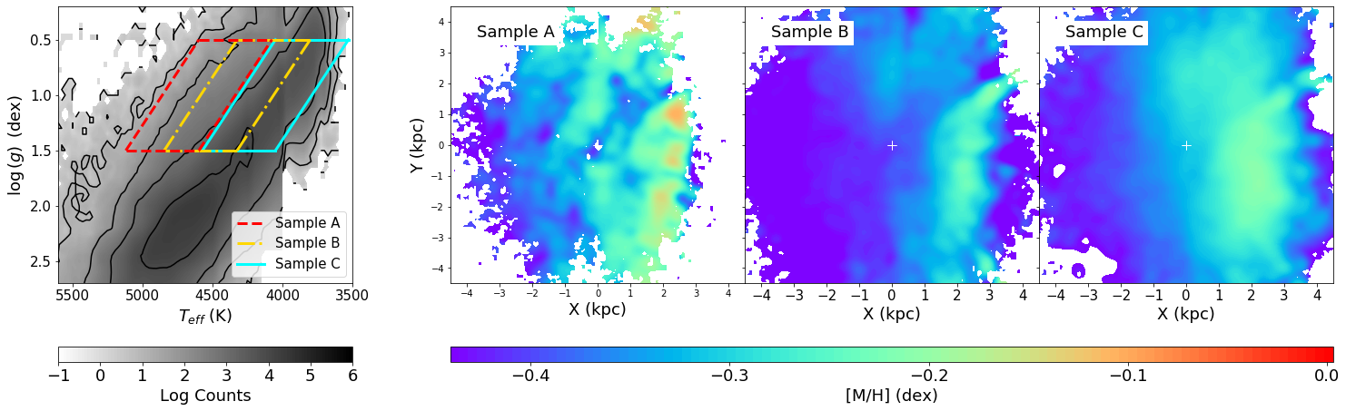
Figure 1: Chemical inhomogenities in the Galactic disc for three different samples. Left panel: Selection of Sample A, B and C in the Kiel diagram. Right panels: Mean metallicity in heliocentric coordinates for Sample A, B, and C (from left to right, respectively) in the Galactic plane. The position of the Sun is shown by the white cross in (X,Y)=(0 kpc, 0 kpc); the Galactic center is to the right; Galactic rotation is going clockwise.

It has been known for several decades that the disc of the Milky Way contains large-scale non-axisymmetric features, including the spiral arms and a central bar (see e.g. Georgelin & Georgelin, 1976; Okuda et al., 1977; Shen & Zheng, 2020; Gaia Collaboration, Drimmel et al., 2022, and references threin), which can play an important role in the disc’s evolution, and are expected to leave their signature in the observed properties of the stars.

Several models have tried to explain the behaviour of spiral arms in disc galaxies, although their dynamical nature and physical origin still remain unknown. Spiral arms have been proposed to induce large-scale shock waves that trigger the gravitational collapse of gas clouds, enhancing star formation (Roberts, 1969). They can also induce radial migration of stars (Lynden-Bell & Kalnajs, 1972; Sellwood & Binney, 2002; Schönrich & Binney, 2009a, b; Roškar et al., 2012), and trap or scatter stars close to orbital resonances (Contopoulos & Grosbol, 1986). As a consequence, they can generate variations in the mean chemical composition of stars in the arm and inter-arm regions (Minchev et al., 2012; Kordopatis et al., 2015; Grand et al., 2016; Khoperskov et al., 2018; Spitoni et al., 2019; Khoperskov & Gerhard, 2021).

Mapping the spatial distribution of metals within galaxies therefore represents a key aspect to study the processes of chemical enrichment and mixing in the interstellar medium. An extensive review of the chemical enrichment of galaxies across the cosmic epochs can be found in Maiolino & Mannucci (2019) (see also references therein). In external galaxies, several works have found evidence of azimuthal variations in the mean chemical composition of stars (e.g. Sánchez-Menguiano et al., 2016; Ho et al., 2017; Vogt et al., 2017). Recently, using data from the PHANGS–MUSE survey (Emsellem et al., 2022), Williams et al. (2022) found that most of the star-forming galaxies considered in their sample showed significant 2D metallicity variations.

In the Milky Way, chemical inhomogenities were explored by several studies. Balser et al. (2011) analyzed the oxygen distribution of HII regions in the Galactic disc, divided their sample into three Galactic azimuth bins, and found that the corresponding radial gradients were significantly different. Chemical inhomogeneities in iron and oxygen were also found in Cepheids (Pedicelli et al., 2009; Genovali et al., 2014; Kovtyukh et al., 2022). Large metallicity variations were also found in the interstellar medium (De Cia et al., 2021). By combining data from HII regions, Cepheids, B stars and red supergiants, Davies et al. (2009) presented evidence for large azimuthal variations ($\sim$ 0.4 dex) in oxygen, magnesium and silicon on a scale of few kpc in the inner Galactic disc. On the other hand, using APOGEE red-clump stars, Bovy et al. (2014) constrained azimuthal variations in the median metallicity to be $\leq$ 0.02 dex in the region covered by their sample. Using the large spectroscopic survey RAVE and the Geneva Copenhagen Survey, Antoja et al. (2017) analyzed stars in a cylinder of 0.5 kpc radius centered on the Sun, and found asymmetric metallicity patterns in velocity space.

Recently, Gaia Data Release 3 (hereafter DR3, Gaia Collaboration, Vallenari et al., 2022) published the largest stellar catalog with chemical abundances, atmospheric parameters and radial velocities ever created. Radial Velocity Spectrometer (RVS) data were parameterised by the General Stellar Parameteriser - spectroscopy (GSP-Spec) module (Recio-Blanco et al., 2022), delivering chemo-physical parameters for 5.6 million stars over the entire sky. Gaia Collaboration, Recio-Blanco et al. (2022) observed azimuthal variations in red giant branch stars, but didn’t present quantitative results or in-depth discussions on their origin.

Thanks to the large number of chemical and astrometric measurements, as well as Gaia’s all-sky sampling, it is now possible to map chemical inhomogeneities in the Milky Way’s disc as never before, with the goal of detecting the possible signature left by the Galactic spiral arms in the stellar metallicity.

The Letter is structured as follows: in Section 2 we describe the datasets; in Section 3 we present our results; in Section 4 we discuss our findings and future perspectives.

2 Data selection

In this study, we use the main stellar atmospheric parameters (effective temperature $T_{\rm eff}$, surface gravity log($g$), global metallicity [M/H]) derived from Gaia RVS spectra by the GSP-Spec module, to select tracers of the disc population and map large-scale chemical inhomogeneities in our Galaxy. The quality constraints on spectroscopic and astrometric measurements (as well as a Toomre kinematical selection) are detailed in Appendix A.

To serve our purpose, we focus on giant stars, as they are intrinsically bright, and therefore allow us to sample a relatively large volume of the Galactic disc. Also, taking advantage of the large number of high-quality chemical measurements for these stars, a robust statistical analysis can be performed, thanks to high signal-to-noise spectra.

Figure 1 (left panel) shows the portion of the Kiel diagrams populated by the giant stars in our selected sample. Here we select stars brighter than the red clump (which is located at approximately log($g$)$\simeq$ 2.3 and $T_{\rm eff}$$\simeq$ 4750 K), to avoid selection function effects due to the superposition of different stellar populations (see Section 4 of Gaia Collaboration, Recio-Blanco et al., 2022). Indeed, such effects can cause artefacts when investigating radial gradients, which might be erroneously interpreted as signatures of the spiral arms. Selected areas in Fig. 1 (left panel) define three different subsamples (details in Appendix A), which cover different portions of the red giant branch. Additionally, we apply a vertical cut $|Z|=|d\sin{b}|<0.75$ kpc, where $b$ is the galactic latitude and $d$ is the heliocentric distance according to the geometric model by Bailer-Jones et al. (2021). The adopted samples are here labelled as A, B, and C, and contain respectively 19 340, 151 139, and 346 570 stars.

The portion of the Kiel diagram covered by our three samples is expected to be populated by stars of different ages. Both theoretical considerations (based on isochrones) and empirical evidence (based on spatial distribution and stellar kinematics) indicate that Sample A is expected to be typically younger than the other two samples (more details in Appendix B). For instance, the comparison between the selected areas on the Kiel diagram and the PARSEC isochrones (Bressan et al., 2012; Chen et al., 2014, 2015; Tang et al., 2014; Pastorelli et al., 2019) for metallicities between $[M/H]=$ 0 dex and $[M/H]=$-0.5 dex suggests that Sample A should mostly contain stars younger than 100-300 Myr (taking into account typical uncertainties on $T_{\rm eff}$  and log($g$)), while Sample C should be dominated by much older stars, i.e. $\gtrsim$ 1 Gyr (see Fig. 4). On the other hand, Sample B is expected to be intermediate between the two, containing a mixture of young and old stellar populations. As will be shown in the following, the different content of the three samples will determine remarkable differences in their observed metallicity maps.

3 Results

Figure 1 (right panels) shows the maps of the mean metallicity $\langle\,$[M/H]$\,\rangle$ in the Galactic plane for Samples A, B and C, using a smoothing Gaussian kernel with a bandwidth of 175 pc (see Appendix C). As discussed in the following, the three maps exhibit both similarities and differences. On a large scale, stars are typically more metal-rich toward the inner parts of the Galaxy for all three samples. This is in agreement with previous observations of radial metallicity gradients in the Galactic disc (e.g. Genovali et al., 2014; Gaia Collaboration, Recio-Blanco et al., 2022), and also expected from the inside-out formation scenario (Bird et al., 2013; Matteucci, 2021). However, the maps also present smaller-scale metallicity inhomogenehities. The relative importance, extent, and shape of the observed inhomogeneities vary for the three different samples. Sample A exhibits three, possibly four, metal-rich elongated features, that diagonally cross the portion of the XY-plane covered by our dataset. One feature extends approximately from (X,Y)=($-$1.5 kpc, 3 kpc) to ($-$3 kpc, $-$1 kpc). A second feature stretches from (X,Y)=(1 kpc, 3.5 kpc) to (X,Y)=($-$1.5 kpc, $-$1 kpc), and then continues almost vertically out to (X,Y)=($-$1.5 kpc, $-$3 kpc). A third feature (which possibly contains multiple segments) extends from (X,Y)=(2.5 kpc, 1 kpc) to (X,Y)=(1 kpc, $-$4 kpc). This pattern becomes progressively less evident as we move from Sample A to Sample B and C. In Sample C, the elongated features disappear almost completely, and simply result in an observed asymmetry about the Sun of stars at $X\simeq$ 0 kpc, typically more metal rich at $Y>0$ kpc than at $Y<0$ kpc. While such asymmetry was already noted by Gaia Collaboration, Recio-Blanco et al. (2022) in their RGB sample, the scenario presented in this contribution indicates that it might represent a remnant of the spiral arms chemical signature.

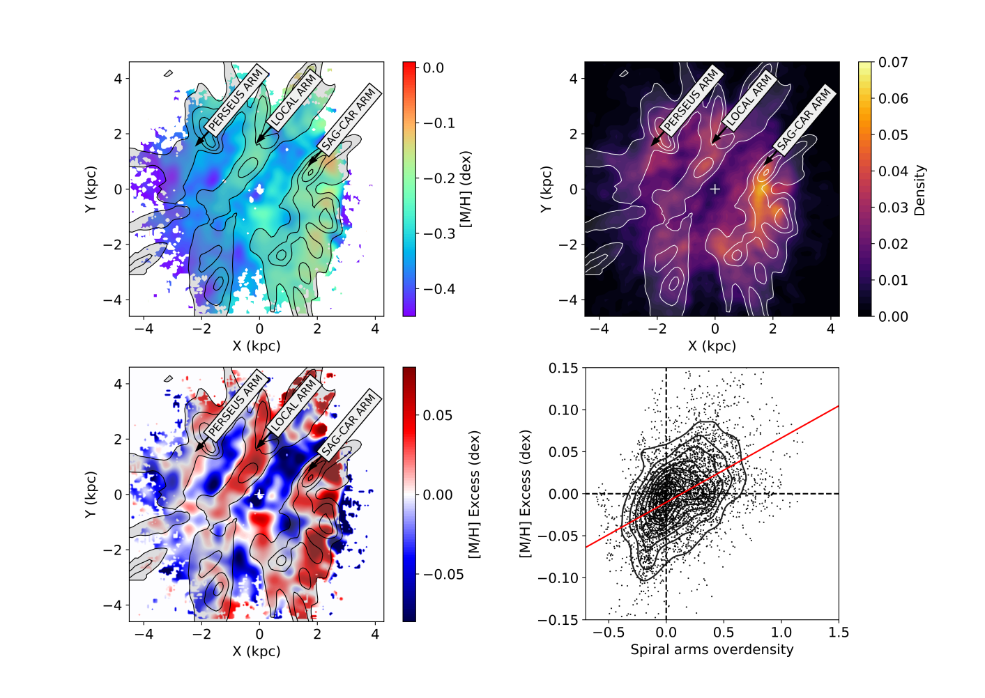
Figure 2: Correlation between the observed metal-rich features in Sample A and the segments of the nearest spiral arms in the Galaxy. Upper left panel: Map of the mean metallicity in the Galactic plane for Sample A shown in Fig. 1, but now compared to the position of the spiral arms from Upper Main Sequence stars (UMS) in Poggio et al. (2021), shown as grey shaded areas. The labels show the position of the Perseus arm, the Local (Orion) arm and the Sagittarius-Carina arm based on the UMS map. Upper right panel: bivariate kernel density estimation for Sample A using an Epanechnikov kernel with a smoothing length of 250 pc. The contours are the same as the upper left panel. Lower left panel: Same as Upper panels, but now showing the metallicity excess. Regions with positive (negative) metallicity excess are more metal-rich (-poor) than the average (see text for a detailed explanation). Lower right panel: Using the map shown in the lower left panel, the overdensity of the spiral arms vs. the metallicity excess is shown for each pixel (black dots). When the spiral arm overdensity is $>0$, the region can be considered belonging to a spiral arm, whereas regions with $<0$ can be considered interarm regions. Black contours show the distribution of the pixels in the spiral arms overdensity vs. metallicity excess space. The red line shows a linear fit to the points.

Figure 2 (upper left panel) shows again the mean metallicity for Sample A, but now compared to the position of the spiral arms in the Galaxy as mapped by Upper Main Sequence UMS stars in Poggio et al. (2021), shown as grey shaded areas and black contours, indicating (from left to right) the segments of: the Perseus arm, the Local (Orion) arm, and the Sagittarius-Carina (Sag-Car) arm (the latter contour possibly containing the Scutum arm).

In the upper right panel of Fig. 2, we can see the spatial distribution of sources in Sample A, obtained with an Epanechnikov kernel density estimator with a bandwidth of 250 pc. White contours show again the position of the nearest spiral arms from UMS stars. As we can see, Sample A traces well the position of the spiral arms, confirming that it contains typically young stars.

To better analyse and map chemical inhomogeneities in the Galactic disc, we define a new variable, called Metallicity Excess, defined as $\langle\,\rm{[M/H]}\,\rangle_{\rm{loc}}-\langle\,\rm{[M/H]}\,\rangle_{\rm{large}}$, where $\langle\,[\rm{M/H}]\,\rangle_{\rm{loc}}$ and $\langle\,[\rm{M/H}]\,\rangle_{\rm{large}}$ represent the mean metallicity smoothed on a local or large scale, respectively. The smoothing is performed as described in Appendix C. The lower left panel of Fig. 2 shows the obtained Metallicity Excess for Sample A if we adopt for the local smoothing the same value chosen for the mean metallicity in the upper left panel of Fig. 2 (i.e. $\langle\,[\rm{M/H}]\,\rangle_{\rm{loc}}=\langle\,[\rm{M/H}]\,\rangle$), and for the large-scale metallicity a scale-length of 5 times the value adopted for the local smoothing. The red (blue) regions in the Metallicity Excess map should be interpreted as places where the stars are more metal-rich (-poor) than the average.

We therefore study the correlation between the observed metal-rich regions and the geometry of the spiral arms by dissecting the XY map (e.g. lower left panel of Fig. 2) in pixels of 0.3 kpc width. For each pixel, we consider the spiral arms overdensity (calculated as described in Poggio et al., 2021) and the Metallicity Excess. The bottom right panel of Fig. 2 shows the correlation between these two quantities (every black dot corresponds to a pixel in the XY map). The red line shows a linear fit to the black dots. As we can see, regions located in correspondence of the spiral arms (i.e. with overdensity larger than 0) tend to be more metal-rich than the average (i.e. with a Metallicity Excess larger than 0). To quantify the correlation between these two variables, we calculate Kendall’s correlation coefficient $\tau_{B}=0.38$, which can be considered as an indication of strong positive correlation. Therefore, the elongated metal-rich features observed in Sample A appear to be statistically correlated with the position of the spiral arms in the Galaxy.

It should be noted, however, that there are some exceptions. For instance, the enhancement of metallicity at approximately (X,Y)=( 0 kpc, $-$1 kpc) does not seem to correspond to an overdensity in the spatial distribution. The comparison between our map and the data from Hottier et al. (2021) reveals that it might correspond to the Vela Molecular Ridge. This region can be seen as a dust enhancement in the maps of Lallement et al. (2019); Vergely et al. (2022), and possibly prevents us from seeing an overdensity in the spatial distribution of stars (for both Sample A and UMS stars, see the upper right panel in Fig. 2).

Furthermore, it is interesting to note that not all the regions in the spiral arms exhibit the same chemical behaviour: the metallicity excess seems to be typically high in the Sag-Car arm and in the upper part (Y¿0) of the Local arm, but seems to be milder in the lower part of the Local arm (Y¡0) and the Perseus arm (Y $\lesssim$ 1 kpc).

Figure 3 shows the impact of the above-described metal-rich features on the observed metallicity gradient in the Galactic disc. To explore the metallicity variations in the disc, we dissect the Galactic plane into slices of 10^∘ width in Galactic azimuth $\phi$. For each slice, we then show the median metallicity for Sample A and Sample C. Sample B presents an intermediate behaviour between Sample A and C (here not shown to preserve the clarity of the Figure). As we can see, Sample A presents some peaks of higher metallicity, superimposed on a global decrease as a function of $R$, here calculated assuming a distance to the Galactic center $R_{\odot}=8.249$ kpc (Gravity Collaboration et al., 2021). Based on bootstrap uncertainties, the peaks deviate more than 3-sigma from a linear decrease as a function of Galactic radius, indicating that the radial metallicity gradient is dominated by chemical undulations, that reach maximum deviations of $\sim$ 0.05-0.1 dex. In this context, the observed peaks can be interpreted as the projection on the radial direction of the metal-rich features observed in the XY maps. For Sample C, on the other hand, a relatively smooth decrease of the median metallicity as a function of $R$ is apparent. The slopes of the radial metallicity gradients for different azimuthal bins can be found in Table 1. As we can see, the radial metallicity gradient gradually varies depending on azimuth, and becomes gradually steeper for $\phi<0^{\circ}$.

Additional tests to verify the robustness of our results can be found in Appendix E.

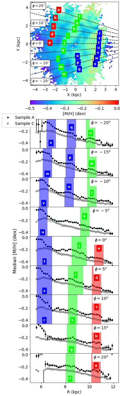
Figure 3: Impact of the observed chemical inhomogeneities on the Galactic gradients. Upper panel: Map of the mean metallicity in the Galactic plane for Sample A, with overlaid azimuthal slices of 5^∘, from $\phi=-20^{\circ}$ to $\phi=20^{\circ}$. Lower panel: median metallicity as a function of Galactocentric radius $R$ for different slices in Galactic azimut $\phi$ for Sample A (filled dots) and Sample C (open dots). Regions that might be associated with the Perseus (red, letters ‘a’–‘e’), Local (green, ‘f’–‘n’), and Sagittarius/Scutum (blue, ‘o’–‘x’) arms are shown as colored regions both in the upper and lower panels.

Table 1: Radial gradient for Sample C in different azimuthal bins, as shown in Fig. 3, assuming a linear model. Only stars with $R>6.5$ kpc are here considered, to avoid selection effects in the inner regions due to extinction, as well as $R<11.5$ kpc, to avoid low statistics regions. The corresponding table for Sample A and B is not presented here due to the spiral arms-related metallicity variations, which are invalidating the assumption of a linear model.

$\phi$ (deg)	Slope (dex kpc-1)	Intercept (dex)
$-$20 $\pm$ 5	$-$0.054 $\pm$ 0.001	0.15 $\pm$ 0.01
$-$15 $\pm$ 5	$-$0.052 $\pm$ 0.002	0.14 $\pm$ 0.01
$-$10 $\pm$ 5	$-$0.047 $\pm$ 0.002	0.09 $\pm$ 0.02
$-$5 $\pm$ 5	$-$0.046 $\pm$ 0.002	0.09 $\pm$ 0.01
0 $\pm$ 5	$-$0.047 $\pm$ 0.001	0.09 $\pm$ 0.01
5 $\pm$ 5	$-$0.046 $\pm$ 0.001	0.09 $\pm$ 0.01
10 $\pm$ 5	$-$0.043 $\pm$ 0.001	0.06 $\pm$ 0.01
15 $\pm$ 5	$-$0.039 $\pm$ 0.001	0.04 $\pm$ 0.01
20 $\pm$ 5	$-$0.035 $\pm$ 0.002	0.01 $\pm$ 0.01

4 Discussion and Conclusion

Taking advantage of the new Gaia DR3 data, we have mapped the mean metallicity in the Galactic disc out to 3-4 kpc of the Sun for three different samples of bright giant stars. We found evidence of chemical inhomogeneities, which manifest themselves as statistically significant undulations on top of the expected radial metallicity gradients. The appearance and magnitude of the detected inhomogeneities are different for the three considered samples, being more structured and pronounced for the sample containing hotter (and a larger relative fraction of young) stars. In this sample, three (possibly four) extended metal rich features are detected, which appear to be statistically correlated with the position of the spiral arms (independently derived from previous works). Such connection points to the spiral arms as a plausible origin for the observed metal-rich features.

It is interesting to compare our maps of the mean metallicity in the Milky Way’s disc to the results based on external spiral galaxies. For the galaxy HCG91c, Vogt et al. (2017) found that the chemical enrichment of the interstellar medium proceeds preferentially along spiral structures, and less efficiently across them, in agreement with our results. Williams et al. (2022) considered a sample of 19 galaxies, for which detected significant chemical variations in most cases, but found no clear signs of enrichment along the spiral arms. On the other hand, Sánchez-Menguiano et al. (2020) detected the presence of more metal-rich HII regions in the spiral arms with respect to the corresponding interarm regions for a large subsample of galaxies, in agreement with the maps presented here for the Milky Way.

While the observed inhomogeneities are more pronounced and structured for the youngest stars, azimuthal variations in the old stellar populations also deserve some discussion. The oldest stars considered here (Sample C) present a metallicity gradient that changes with Galactic azimuth, with a slope that varies from $\sim-$0.054 dex kpc^-1 to $\sim-$0.035 dex kpc^-1. To our knowledge, this is the first time that such azimuthal dependence is shown for old stellar populations, both in the Milky Way and in external galaxies. The slopes obtained here for Sample C using different azimuthal bins are in good agreement (considering the uncertainties) with those from the giant stars at all azimuths in the Galactic plane in Gaia Collaboration, Recio-Blanco et al. (2022) (see their Table 1), which have a slope of $-$0.055 $\pm$ 0.007 dex kpc^-1 above the plane, and $-$0.057 $\pm$ 0.007 dex kpc^-1 below the plane. Previous works reported slopes for thin disc (i.e. low $\alpha-$sequence) field stars ranging from $\sim-$0.053 dex kpc^-1 to $\sim-$0.068 dex kpc^-1 (Bergemann et al., 2014; Recio-Blanco et al., 2014; Hayden et al., 2015; Anders et al., 2017).

Recently, Hawkins (2022) mapped azimuthal variations in the Galactic disc, using both Gaia DR3 data and a sample OBAF-type stars from the LAMOST survey published by Xiang et al. (2022). Using the LAMOST sample, the author found azimuthal structure on top of the radial gradient, which doesn’t necessarily follow the spiral arms. On the other hand, using Gaia DR3, Hawkins (2022) found good agreement with the results presented in this Letter, finding that giant stars near the spiral arms typically contain more metals than those in the interarm regions. The author suggests that the discrepancy between the two samples can be due to the fact that either LAMOST data is too local to see the overall structure, or that azimuthal structure depends strongly on age, selection function and spectral type of the tracer population.

Several works available in the literature can offer a theoretical framework for the obtained observational results. Using high-resolution $N$ -body simulations, Khoperskov et al. (2018) showed that kinematically hot and cold stellar populations in the Galactic disc react in a different way to a spiral arm perturbation, naturally leading to azimuthal variations in the mean metallicity of stars in the simulated disc (based on the assumption that younger stars typically tend to have higher metallicity and smaller random motions than the older stellar components, see for example Holmberg et al., 2007). Figure 4 in Khoperskov et al. (2018) shows the azimuthal metallicity variations at different times of the simulation for three different initial metallicity profiles. They found that the spiral arms locii typically tend to be more metal-rich than the interarm-regions. Their predictions are in good agreement with the observations presented in this work.

In the future, a detailed modelling will be crucial to fully explain the observed chemical inhomogeneities in the Galactic disc. Chemo-dynamical evolution models should be adopted to interpret the impact of the spiral arms on chemical variations in the Galactic disc, and to understand how different mechanisms can influence the observed present-day chemical abundance patterns (e.g. Roškar et al., 2012; Grand et al., 2016; Minchev et al., 2018; Spitoni et al., 2019, 2022a, 2022b; Carr et al., 2022). Future works comparing observations from Gaia DR3 and ground-based surveys to sophisticated theoretical models will be able to show further insights on the evolutionary processes that shaped the present-day appearance of the Milky Way’s disc.

Appendix A Data quality cuts and selection

We select Gaia DR3 sources with atmospheric parameters (available through the gaiadr3.astrophysical_parameters table), radial velocities, and 5-parameters astrometric solution having quality index ruwe $<1.4$ (Lindegren 2018). In addition, Gaia duplicated sources are excluded from the sample. As for the GSP-Spec parameters, we reject objects based on their metallicity uncertainty and GSP-Spec quality flags (Recio-Blanco et al. 2022) reporting on the degree of biases from line broadening and radial velocity errors affecting [M/H], flux noise, extrapolation on stellar atmospheric parameters, as well as KM-type stars.

The definition of the working sample is as follows:

 [M/H]_unc<0.5 & vbroadM<2 & vradM<2 &
 fluxNoise<4 & extrapol<3 & KMtypestars<2
 astrometric_params_solved = 31 & ruwe < 1.4
 & duplicated_source == false

From the Gaia archive the following query provides the data set employed:

SELECT g.*, ap.teff_gspspec,
ap.logg_gspspec, ap.mh_gspspec
FROM gaiadr3.gaia_source AS g
INNER JOIN gaiadr3.astrophysical_parameters AS ap
ON g.source_id = ap.source_id
WHERE (
((mh_gspspec_upper-mh_gspspec_lower)<0.25)
AND ((flags_gspspec LIKE ‘__0%’)
OR (flags_gspspec LIKE ‘__1%’))
AND ((flags_gspspec LIKE ‘_____0%’)
OR (flags_gspspec LIKE ‘_____1%’))
AND ((flags_gspspec LIKE ‘______0%’)
OR (flags_gspspec LIKE ‘______1%’)
OR (flags_gspspec LIKE ‘______2%’)
OR (flags_gspspec LIKE ‘______3%’))
AND ((flags_gspspec LIKE ‘_______0%’)
OR (flags_gspspec LIKE ‘_______1%’)
OR (flags_gspspec LIKE ‘_______2%’))
AND ((flags_gspspec LIKE ‘____________0%’)
OR (flags_gspspec LIKE ‘____________1%’))
) AND g.astrometric_params_solved = 31
AND g.ruwe < 1.4

Additionally, objects without $d_{Geo}$ distances were discarded.

For the obtained sample, we calculate the Galactocentric coordinates $R,\phi,Z$ and the corresponding velocities $V_{R},V_{\phi},V_{Z}$ following the same conventions and parameters adopted in Gaia Collaboration, Recio-Blanco et al. (2022). We apply a cut —Z—¡0.75 kpc, as we are mainly interested in selecting disc stars. To this end, we also apply a kinematical cut based on the Toomre diagram (see for example Bensby et al. 2003, 2014; Re Fiorentin et al. 2019, 2021; Gaia Collaboration, Recio-Blanco et al. 2022; Gaia Collaboration, Creevey et al. 2022) in order to remove possible halo contaminants:

$$\sqrt{V_{R}^{2}+V_{Z}^{2}+(V_{\phi}-V_{0})^{2}}<210\,\,\,\mbox{km\leavevmode\nobreak\ s}^{-1},$$ (1)

where $V_{0}=238.5$ km s^-1 is the velocity of the local standard of rest at the Sun’s position, based on Gravity Collaboration et al. (2021) and Schönrich et al. (2010).

Finally, we select different populations of RGB stars in the log($g$)-$T_{\rm eff}$ plane of the Kiel diagram. This is accomplished by selecting stars in the three boxes shown in the left panel of Fig. 1, that is:

logg < 1.5 & logg > 0.5 &
(logg > (coeff*teff + interc_left)) &
(logg < (coeff*teff + interc_right))

where coeff= 0.00192 $\rm{dex\,K}^{-1}$ is the adopted slope, chosen to follow the natural inclination of the RGB branch (as done also for the selection of the massive sample in Gaia Collaboration, Recio-Blanco et al. 2022), whereas the intercept of the two inclined lines, delimiting the selected regions on the left and right side, are: interc_left = -8.3 + $\Delta$ dex and interc_right = -7.3 + $\Delta$ dex, where $\Delta$ = 0, 0.5 and 1 for Sample A, B and C, respectively.

Appendix B Sample characterization

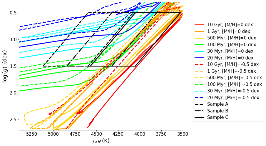
Figure 4: PARSEC isochrones for different metallicites and ages, compared to the regions of the Kiel diagram selected here for Sample A, B and C.

Figure 5: Distribution of azimuthal velocities $V_{\phi}$ for Sample A, B, and C. The histogram is normalized so that the area under the histogram integrates to 1 for all three samples.

Here we performed some tests to further explore the content of Sample A, B and C. First of all, we compared our selected areas of the Kiel diagram with the prediction from the PARSEC isochrones for different metallicities (Bressan et al. 2012; Chen et al. 2014, 2015; Tang et al. 2014; Pastorelli et al. 2019). Figure 4 shows the isochrones for 10 Gyr, 1 Gyr, 500 Myr, 100 Myr, 30 and 20 Myr, for both solar metallicity [M/H]=0 dex and [M/H]=-0.5 dex. It should be noted that effective temperatures from GSP-Spec have been found to be in agreement with those from the isochrones (see Section 10.2 of Recio-Blanco et al. 2022), and no important bias as been found with the literature. As we can see in Fig 4, in the region covered by Sample A, only isochrones for 100 Myr or younger are present. Of course, in real data, we do expect some contamination from older stars, given that uncertainties will tend to blur the distribution. Nevertheless, the fact that Sample B and C contain stars typically older than those in Sample A is supported by the location of the isochrones in the Kiel diagram.

Further indications can be also found empirically. Although ages can be also inferred for stars (e.g. Kordopatis et al. 2022), here we simply use stellar kinematics as a proxy for the typical age of the sample. For Sample A, B and C, respectively, the velocity dispersions are: $\sigma_{V_{Z}}=(19.5,21.8,23.6)$ km s^-1, $\sigma_{V_{R}}=(28.6,35.1,38.9)$ km s^-1, $\sigma_{V_{\phi}}=(26.6,26.9,29.0)$ km s^-1. Figure 5 shows the distribution of the azimuthal velocities $V_{\phi}$. As we can see, the distribution of stars in Sample A presents a prominent peak at high azimuthal velocity ($\sim$ 230-240 km s^-1). On the contrary, Sample B and Sample C present a broader distribution, with a large fraction of stars at low $V_{\phi}$, as would be expected as a consequence of the asymmetric drift for a kinematically hot stellar population.

Appendix C Bivariate smoothing

For a given position (X,Y) in the Galactic plane, we calculate the local smoothed metallicity:

$$\langle\,{\rm[M/H]}\,\rangle_{\rm loc}\,(X,Y)=\frac{\sum^{N}_{i}{\rm[M/H]}_{i}\,K\left(\frac{X-X_{i}}{h_{X}}\right)\,K\left(\frac{Y-Y_{i}}{h_{Y}}\right)}{\sum^{N}_{i}K\left(\frac{X-X_{i}}{h_{X}}\right)\,K\left(\frac{Y-Y_{i}}{h_{Y}}\right)}\quad,$$ (2)

where $N$ is the total number of stars in the sample, $X_{i}$ and $Y_{i}$ are the X- and Y-coordinates of the $i$-th star of the sample, $K$ is a Gaussian kernel

$$K\biggl{(}\frac{X-X_{i}}{h_{X}}\biggr{)}=\frac{1}{\sqrt{2\pi}\,h_{X}}\exp{\Biggl{(}-\frac{1}{2}\Biggl{(}\frac{(X-X_{i})}{h_{X}}\Biggr{)}^{2}\Biggr{)}}$$ (3)

with a scale-length $h_{X}$ (and similarly for the Y-coordinate). In this work, local smoothed metallicity (see Fig. 1, right panels) is shown using a scale-length of 0.175 kpc. As discussed in the main text, the metallicity excess is calculated by taking the difference of the local metallicity (i.e. Equation 2, assuming a scale-length of 0.175 kpc) and the metallicity on a large scale (i.e. again using Equation 2, but now adopting a scale-length 5 times larger than the one used for the local metallicity).

Appendix D Azimuthal variations

Figure 6 shows a projection of the observed metal-rich spiral features when the Galactic plane is cut into Galactocentric rings. For each ring, we show the azimuthal variations for both Sample A and Sample C, calculated as the median metallicity as a function of azimuth, after subtracting the median metallicity of the sample in each ring. We note that the azimuthal variations depend on the adopted sample, being more prominent for Sample A; typically, they do not exceed 0.08 dex. The amplitude and location of the observed peaks depend on how the rings are selected with respect to the spiral arms’ geometry.

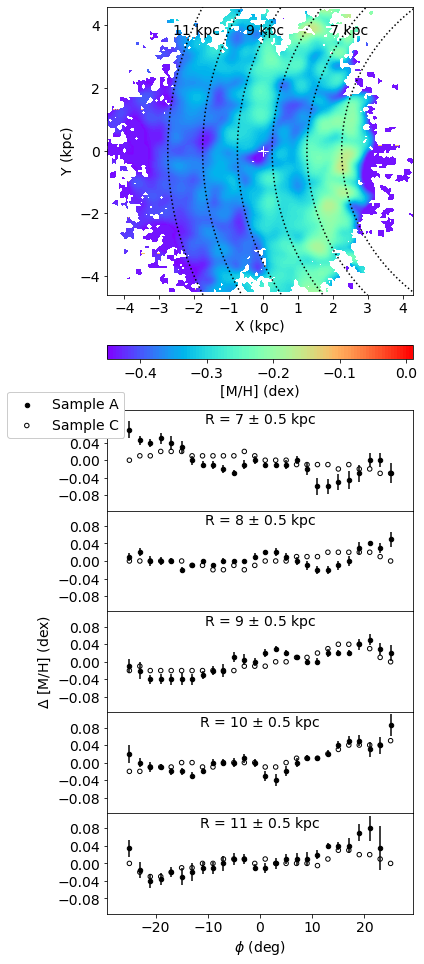
Figure 6: Impact of the observed chemical inhomogeneities on azimuthal variations. Upper panel: Map of the mean metallicity in the Galactic plane for Sample A, with overlaid rings of constant Galactocentric radius at $R=6,7,8,9,10$ and $11$ kpc. Lower panels: median metallicity for sample A and C (filled/open dots, respectively) as a function of Galactic azimuth $\phi$ for different rings in $R$ (as specified in each panel), after the median metallicity of the stars for each ring is subtracted.

Appendix E Additional tests

Here we present some additional tests that we perform to verify the robustness of our results.

First, we checked the quality of the astrometric measurements in our selected stars. For Sample A, 99.7 % of the stars have a parallax signal-to-noise greater than 5. For those stars, as a further check, we constructed a map using distances inferred by the inverse of the parallax, obtaining consistent results.

As an additional test, we selected only the stars satisfying the criteria on Gaia DR3 astrophysical parameters listed for the high-quality sample in Gaia Collaboration, Recio-Blanco et al. (2022). In this case, the chemical signature of the spiral arms is still present, but the entire map is shifted toward more metal-rich values, as expected (given that more metal-rich stars are more likely to be included in the high-quality sample).

To test the possible contribution from Asymptotic Giant Branch (AGB) stars, we cross-matched our three samples with the long-period variables catalog available in Gaia DR3 gaiadr3.vari_long_period_variable. We found that, for all three samples, the percentage of AGB stars from that catalog is less than 0.2 %.

Our maps are also quite robust against the selection of the regions in the Kiel diagram. Indeed, a change in the shape of the selection leave the maps almost unchanged - although, of course, a significant shift in $T_{\rm eff}$ (or log($g$)) can make an impact, as discussed in the main text.

Finally, we test other spiral arms maps. The spiral arms contours used in the main text are from Poggio et al. (2021), which relies on distances calculated as described in Poggio et al. (2018). As a test, we also used the spiral arms overdensity map from Gaia Collaboration, Drimmel et al. (2022), where the $d_{Geo}$ distances are adopted from Bailer-Jones et al. (2021), as well as the one based the sample from Zari et al. (2021) (which used astro-kinematic distances), always obtaining consistent results.