The $f_{0}(1370)$ controversy from dispersive meson-meson scattering data analyses

Abstract

We establish the existence of the long-debated $f_{0}(1370)$ resonance in the dispersive analyses of meson-meson scattering data. For this, we present a novel approach using forward dispersion relations, valid for generic inelastic resonances. We find its pole at $\left(1245\pm 40\right)-i\,\left(300^{+30}_{-70}\right)$ MeV in $\pi\pi$ scattering. We also provide the couplings as well as further checks extrapolating partial-wave dispersion relations or with other continuation methods. A pole at $\left(1380^{+70}_{-60}\right)-i\,\left(220^{+80}_{-70}\right)$ MeV also appears in the $\pi\pi\to K\bar{K}$ data analysis with partial-wave dispersion relations. Despite settling its existence, our model-independent dispersive and analytic methods still show a lingering tension between pole parameters from the $\pi\pi$ and $K\bar{K}$ channels that should be attributed to data.

Introduction.– Quantum Chromodynamics (QCD) was established as the theory of strong interactions almost 50 years ago, but its low-energy regime, particularly the lightest scalar spectrum, is still under debate—see Peláez (2016); Peláez and Rodas (2022) and the “Scalar Mesons below 2 GeV” note in the Review of Particle Physics Zyla et al. (2020) (RPP). This may be surprising, since light scalars are relevant for nucleon-nucleon interactions, final states in heavy hadron decays, CP violation studies, etc. Also, isoscalar-scalar mesons have the quantum numbers of the vacuum and the lightest glueball, thus becoming crucial for understanding the QCD spontaneous chiral symmetry breaking and the most salient feature of a non-abelian gauge theory spectrum, respectively. Hence, a precise knowledge of this sector is relevant by itself, but also for QCD and the accuracy frontier of Nuclear and Particle Physics.

This debate lingers on because light scalars do not show up as nice resonance peaks, since some of them are very wide and overlap with others, or are distorted by nearby two-particle thresholds. Not being sharp peaks, their shape changes with the dynamics of the process where they appear. Hence, they must be rigorously identified from their process-independent associated poles. These poles appear in the complex $s$-plane of any amplitude $T(s)$ where resonances exist. Here, $s$ is the total CM-energy squared Mandelstam variable. Then, the pole mass $M$ and width $\Gamma$ are defined as $\sqrt{s_{pole}}=M-i\Gamma/2$. The familiar peak-shape only appears in the real axis when the resonance is narrow and isolated from other singularities. Only then, simple Breit-Wigner (BW) approximations, or models like K-matrices or isobar sums, may be justified, but not for the lightest scalars and particularly not for the $f_{0}(1370)$.

Problems identifying light scalars are crudely of two types. The “data problem” is severe in meson-meson scattering, where scalars were first observed, since data are extracted indirectly from the virtual-pion-exchange contribution to meson-nucleon to meson-meson-nucleon scattering. Hence, the initial state is not well defined, leading to inconsistencies in the data and with fundamental principles. In contrast, the initial state is well defined in many-body heavy-meson decays, generically with better statistics and less systematic uncertainty. The “model problem” arises in the search for poles, since analytic continuations are a delicate mathematical problem, particularly for resonances deep in the complex plane. Unfortunately they are often carried out with models (BW, K-matrices, etc), aggravated for many-body heavy-meson decays by “isobar” sums of two-body approximations. Dispersion theory addresses both problems by discarding some inconsistent data, and avoiding model dependencies in the data description and resonance-pole identification.

The RPP Zyla et al. (2020) lists the $\sigma/f_{0}(500)$, $f_{0}(980)$, $f_{0}(1370)$, $f_{0}(1500)$ and $f_{0}(1710)$ scalar-isoscalar resonances below 2 GeV. The longstanding controversy on the existence of the very wide $\sigma/f_{0}(500)$, and the similar strange $\kappa/K_{0}^{*}(700)$, was settled (see Peláez (2016); Peláez et al. (2021)) by precise and unambiguous dispersive determinations of their poles Caprini et al. (2006); García-Martín et al. (2011a); Moussallam (2011); Descotes-Genon and Moussallam (2006); Peláez and Rodas (2020, 2022). The $f_{0}(980)$, very close to $K\bar{K}$ threshold, is firmly established since the 70’s and its pole has also been rigorously determined dispersively García-Martín et al. (2011a); Moussallam (2011). Despite being the narrowest, it illustrates the process-dependence of resonance shapes, by appearing as a dip in the $\pi\pi\rightarrow\pi\pi$ cross section but as a peak in heavy meson decays. The $f_{0}(1500)$ and $f_{0}(1710)$ are also well established. Namely, the RPP estimates less than 10 MeV uncertainties for the $f_{0}(1500)$ mass and width and lists five accurate branching fractions. The $f_{0}(1710)$ has mass and width uncertainties below 20 MeV and six “seen” decay modes.

In contrast, the $f_{0}(1370)$ situation remains controversial (some reviews find enough evidence to consider it well established Bugg (2007) whereas others do not Klempt and Zaitsev (2007); Ochs (2013)). In brief, a scalar-isoscalar state between 1.2 and 1.5 GeV has been reported by several experiments Pawlicki et al. (1977); Cohen et al. (1980); Etkin et al. (1982); Akesson et al. (1986); Gaspero (1993); Adamo et al. (1993); Amsler et al. (1994, 1992); Anisovich et al. (1994); Amsler et al. (1995a, b, c); Abele et al. (1996a, b); Barberis et al. (1999a, b); Bellazzini et al. (1999); Aitala et al. (2001a, b); Abele et al. (2001a, b); Link et al. (2004); Ablikim et al. (2005); Garmash et al. (2005); Cawlfield et al. (2006); Bonvicini et al. (2007); Aaij et al. (2011); d’Argent et al. (2017), but with large disagreements on its parameters and decay channels. However, it was absent in the classic $\pi\pi$ scattering analyses Hyams et al. (1973); Grayer et al. (1974); Hyams et al. (1975); Estabrooks (1979), where a peak or phase-shift motion is not seen. One of our main results here is that we do find such a pole in $\pi\pi\to\pi\pi$ data using rigorous dispersive and analyticity techniques. A pole is also found in coupled-channel theoretical analyses of multiple sources of data, where four meson channels are approximated or included as background or in the quasi-two-body approximation (see for instance the recent Sarantsev et al. (2021) and the very complete analyses Albaladejo and Oller (2008); Guo et al. (2012a, b); Ledwig et al. (2014) using unitarized chiral lagrangians). It has been noted Ropertz et al. (2018); Rodas et al. (2022) that its visibility may be strongly dependent on the source. In general, $f_{0}(1370)$ analyses suffer from some aspects of the “model problem”: parameterization choices, most frequently BW, K-matrices, non-resonant backgrounds and isobars, a priori selection of decay channels, two-body or quasi-two-body approximations, etc. All in all, the RPP places the $f_{0}(1370)$ pole within a huge range, $\left(1200-1500\right)-i\,\left(150-250\right)$ MeV, and lists its decay modes only as “seen”. In addition, despite not being adequate for this resonance, the RPP lists its BW parameters, separating the “$K\bar{K}$ mode” mass determinations, always above $\sim$1.3 GeV, from those of the “$\pi\pi$ mode”, which can be as low as $\sim 1.2$ GeV.

In this work we confirm the existence of the $f_{0}(1370)$, particularly the often missing pole in $\pi\pi\to\pi\pi$ scattering, and provide a rigorous determination of its parameters, by using model-independent dispersive and analytic techniques, similar to those used to settle the $\sigma/f_{0}(500)$ and $\kappa/K_{0}^{*}(700)$ controversies. We study $\pi\pi\to\pi\pi$ and $\pi\pi\to K\bar{K}$ because the most stringent dispersive constraints are those for two-body scattering, particularly for $\pi\pi\rightarrow\pi\pi$, since it is related to itself by crossing and no other processes are needed as input. We will first explain the dispersion relations we use to constrain the data, next the analytic methods to reach the complex poles and finally provide the results and further checks. All numerical and minor details are given in Appendix.

Dispersion relations for $\pi\pi\to\pi\pi,K\bar{K}$.– As usual, we work in the isospin limit. Due to relativistic causality, and since no bound states exist in meson-meson scattering, the amplitude $F(s,t)$, for fixed $t$, is analytic in the first Riemann sheet of the complex-$s$ plane except for a right-hand-cut (RHC) along the real axis from $s=4m_{\pi}^{2}$ to $+\infty$. Crossing this RHC continuously leads to the “adjacent” Riemann sheet, where resonance poles sit. In addition, there is a left-hand-cut (LHC) from $-\infty$ to $s=-t$ corresponding to cuts from crossed channels. Note that the LHC extends up to $s=0$ for forward scattering ($t=0$) and for partial-wave amplitudes. Using Cauchy’s integral formula the amplitude in the first Riemann sheet can be recast in terms of integrals over its imaginary part along the RHC and the LHC.

Customarily, the pole of a resonance with isospin $I$ and spin $J$ is obtained from $f^{I}_{J}(s)$ partial waves. In the elastic case the adjacent sheet is simply the inverse of the first, i.e., $S_{IJ}^{II}(s)=1/S_{IJ}^{I}(s)$. This is how the $\sigma/f_{0}(500)$, $f_{0}(980)$ and $\kappa/K_{0}^{*}(700)$ poles were determined from dispersion relations Caprini et al. (2006); Descotes-Genon and Moussallam (2006); García-Martín et al. (2011a); Moussallam (2011); Peláez and Rodas (2022). However, the $f_{0}(1370)$ lies in the inelastic region and the analytic continuation to the adjacent sheet has to be built explicitly. For this we will use general analytic continuation techniques and to avoid model dependencies we will continue the dispersive output of our Constrained Fits to Data (CFD) García-Martín et al. (2011b), and not the parameterizations themselves.

For $\pi\pi\rightarrow\bar{K}K$ we can use the output of partial-wave hyperbolic dispersion relations, i.e., Roy-Steiner equations, recently extended to 1.47 GeV, whose corresponding CFDs were obtained in Pelaez and Rodas (2018); Peláez and Rodas (2022); Pelaez and Yndurain (2005).

However, the applicability of Roy and GKPY dispersion relations for $\pi\pi\to\pi\pi$ partial waves is limited to $\sim 1.1\,$GeV. This is why we have implemented a novel approach, which is to continue analytically the output of $\pi\pi$ Forward Dispersion Relations (FDR). They can rigorously reach any energy, although in practice have been implemented up to 1.42 GeV García-Martín et al. (2011b); Kaminski et al. (2008); Pelaez and Yndurain (2005), enough for our purposes. The caveat is that we cannot identify the spin of the resonance from FDRs alone. Among the different FDRs, the most precise is that for $F^{00}\equiv(F^{0}+2F^{2})/3$, where $F^{I}(s,t)$ are the $\pi\pi$ scattering amplitudes with definite isospin $I$. Its small uncertainties are due to the positivity of all integrand contributions García-Martín et al. (2011b); Navarro Pérez et al. (2015). For the FDR input we will use the $\pi\pi\to\pi\pi$ CFD from García-Martín et al. (2011b), which describes data and satisfies three FDRs as well as Roy and GKPY equations Roy (1971); García-Martín et al. (2011b). In Fig. 1, we see that the once-subtracted $F^{00}$ FDR is well satisfied in the 1.2 to 1.4 GeV region, dominated by the huge drop due to the $f_{2}(1270)$ resonance.

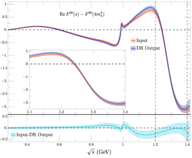
Figure 1: $F^{00}$ Forward Dispersion Relation for the CFD García-Martín et al. (2011b). Note the agreement between input and dispersive output, particularly in the 1.2 to 1.4 GeV region.

Analytic continuation methods.– There are several analytic continuation techniques from a segment in the real axis to the complex plane, such as conformal expansions Yndurain et al. (2007); Caprini (2008), Laurent or Laurent-Pietarinen expansions Švarc et al. (2013, 2014, 2015) sequences of Padé approximants Masjuan and Sanz-Cillero (2013); Masjuan et al. (2014); Caprini et al. (2016); Peláez et al. (2017) or continued fractions Schlessinger (1968); Tripolt et al. (2017); Binosi and Tripolt (2020); Binosi et al. (2022). Some of these methods, like Padé sequences, might require derivatives of very high order at a given point, obtained either from specific functional forms, with additional systematic uncertainty, or numerically, which quickly become unstable. In particular, for the FDRs, as seen in Fig. 2, the dominant $f_{2}(1270)$ pole lies in between the real axis and the $f_{0}(1370)$ pole. To find the subdominant pole requires very high derivatives of the FDR output, rending useless the Padé method, although it will be useful below for other checks. After trying several methods, the most stable both for $\pi\pi$ and $K\bar{K}$ are the continued fractions, $C_{N}$. These are built, as usual, by $N-1$ nested fractions, whose parameters are fixed by imposing $C_{N}(s_{i})=F(s_{i})$ for $N$ real values $s_{i}$ within the domain of interest.

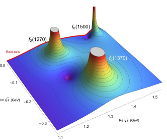
Figure 2: $|F^{00}(s,t=0)|$ obtained from the $F^{00}$ FDR, using as input the CFD in García-Martín et al. (2011b), analytically continued to the lower-half complex $\sqrt{s}$-plane, by means of continued fractions. Note the $f_{2}(1270)$ pole standing between the real axis and the $f_{0}(1370)$ pole, and the $f_{0}(1500)$ pole nearby.

Results.– Let us first describe the continuation of the $\pi\pi\to\pi\pi$ $F^{00}$ FDR output to the complex plane. The $C_{N}$ are calculated from $N=7$ up to 51 equally-spaced energies in the 1.2-1.4 GeV segment. As seen in Fig. 2 for a typical case, we find poles for the $f_{0}(1370)$, $f_{2}(1270)$ and $f_{0}(1500)$. Being able to reproduce the latter is striking since it lies above our segment and the CFD input above 1.42 GeV is not fitted to separated partial-wave data, but is a Regge parameterization only expected to describe the amplitude “on the average”.

In Fig. 3 we show in blue the pole masses (top) and half widths (bottom) for each $N$. Statistical errors are propagated from the CFD input García-Martín et al. (2011b); Kaminski et al. (2008); Pelaez and Yndurain (2005). For each $N$ a systematic uncertainty is added by considering several intervals up to 25 MeV lower in either segment end. Results are very stable for the three resonances and their uncertainties are obtained from a weighted average of the values for each $N$. Note that the energy where the CFD tensor-isoscalar partial-wave phase reaches $\pi/2$ was fixed at 1274.5 MeV, so the $f_{2}(1270)$ pole appears at $1267.5-i\,94\,$MeV, with negligible error. The $f_{0}(1500)$ pole is found at $1523^{+16}_{-10}-i\,\left(52^{+16}_{-11}\right)$ MeV. As these two resonances are not too wide, their pole parameters are similar to their RPP BW values Zyla et al. (2020).

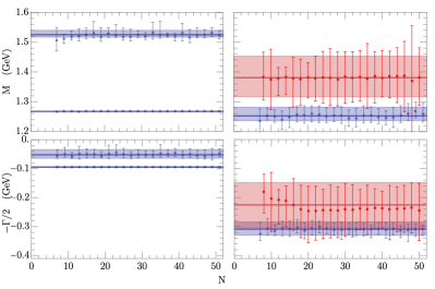
Figure 3: Pole masses ($M$, top) and half-widths ($\Gamma/2$, bottom) of the $f_{2}(1270)$, $f_{0}(1500)$ (Left) and $f_{0}(1370)$ (Right). They are obtained from the output of the $F^{00}$ $\pi\pi\to\pi\pi$ FDR (Blue) or Roy-Steiner $\pi\pi\to K\bar{K}$ dispersive output (Red) analytically continued to the complex plane by a continued fraction of order $N$ (horizontal axis). CFD are used as input. Note the tension between $\pi\pi$ and $K\bar{K}$ $f_{0}(1370)$ determinations.

All in all, in the first row of Tab. 1 we provide the value for the $f_{0}(1370)$ pole parameters, obtained from the $\pi\pi\to\pi\pi$ FDR method. We assign isospin zero to this pole since a consistent but less accurate pole is also found in the $F^{I_{t}=1}=F^{0}/3+F^{1}/2-5F^{2}/6$ FDR, but not in the $F^{+0}=(F^{1}+F^{2})/2$ amplitude. The spin cannot be deduced from FDRs alone, but we will show below that a consistent pole in the $\pi\pi\to\pi\pi$ scalar wave appears with other methods that require further approximations.

Method	$\sqrt{s_{f_{0}(1370)}}$ (MeV)	G (GeV)
FDR+CFD+$C_{N}$	$\left(1253^{+29}_{-16}\right)-i\,\left(309^{+21}_{-25}\right)$	$6.0\pm 0.3$
FDR+Global1+$C_{N}$	$\left(1232^{+29}_{-31}\right)-i\,\left(270^{+47}_{-32}\right)$	$4.9\pm 0.4$
FDR+Global2+$C_{N}$	$\left(1227^{+27}_{-22}\right)-i\,\left(276^{+36}_{-48}\right)$	$4.9^{+0.4}_{-0.3}$
FDR+Global3+$C_{N}$	$\left(1230^{+26}_{-21}\right)-i\,\left(274^{+36}_{-24}\right)$	$4.9^{+0.4}_{-0.5}$
$\mathbf{FDR_{\pi\pi\to\pi\pi}+C_{N}}$	$\mathbf{\left(1245\pm 40\right)-i\,\left(300^{+30}_{-70}\right)}$	$\mathbf{5.6^{+0.7}_{-1.2}}$
$\mathbf{RS_{\pi\pi\to K\bar{K}}+C_{N}}$	$\mathbf{\left(1380^{+70}_{-60}\right)-i\,\left(220^{+80}_{-70}\right)}$	$\mathbf{3.2^{+1.3}_{-1.1}}$

Table 1: $f_{0}(1370)$ pole parameters. First lines, from the $F^{00}$ FDR using as input CFD or global fits to $\pi\pi\to\pi\pi$ data. Fifth line: our estimate from the FDR+$C_{N}$ method. Last line, from partial-wave hyperbolic dispersion relations (RS), using as input constrained fits to $\pi\pi\to K\bar{K}$ data. Both dispersive outputs have been analytically continued to the complex plane with continued fractions. In the first row the coupling $G=|g_{\pi\pi}|$ and in the second $G=|\sqrt{g_{\pi\pi}g_{K\bar{K}}}|$.

Concerning systematic errors, since the $\pi\pi$ CFD is a piece-wise function, we provided later three simple “global” analytic parameterizations Pelaez et al. (2019), almost identical among themselves and to the CFD up to 1.42 GeV. Indeed, they fit the Roy and GKPY equations output in the real axis and complex plane validity domains, together with the FDRs up to 1.42 GeV. By construction, they contain $\sigma/f_{0}(500)$ and $f_{0}(980)$ poles consistent with their dispersive values. From 1.42 GeV up to 2 GeV they describe three different data sets, covering alternative $f_{0}(1500)$ scenarios. Table 1 shows their resulting poles with the same method just applied to the CFD.

For our final $\pi\pi$ FDR result, in line five of Table 1, we first obtain a range covering all global fits, which we combine with the CFD value. In Fig. 4 its position is shown (in blue) in the complex $\sqrt{s}$ plane. It overlaps within uncertainties with the RPP estimate (green area) but our central half-width is $\sim 50$ MeV larger.

The last row of Tab. 1 is our result for the $f_{0}(1370)$ pole position and coupling obtained from the $\pi\pi\to K\bar{K}$ scalar-isoscalar partial-wave Roy-Steiner equation. Its output in the 1.04 to 1.46 GeV segment is continued analytically by continued fractions $C_{N}$. In Fig. 3 we show, now in red, the resulting pole parameters for $N=8$ up to 50. Statistical uncertainties are propagated from the $\pi\pi\to K\bar{K}$ CFD parameterization used as input in the integrals. For each $N$, systematic uncertainties cover the existence of two CFD solutions, the different matching points needed to describe the “unphysical” region between $\pi\pi$ and $K\bar{K}$ thresholds, and a variation of +30 (-30) MeV in the lower (upper) end of the segment. Results are very stable for different $N$ and our final value is obtained by combining the (mass and width) distributions for each $N$, weighted by their uncertainties. Note that, even though the $f_{2}(1270)$ is not present in this wave, the uncertainties are much larger than those from $\pi\pi$. Nevertheless, this confirms in full rigor the $f_{0}(1370)$ pole existence and its scalar-isoscalar assignment.

The pole position from the $\pi\pi\to K\bar{K}$ analysis is shown in red in Fig. 4, fully consistent with the RPP estimate. However, the central mass is two-deviations away from our $\pi\pi\to\pi\pi$ value, and the width about 1 deviation away. Given the negligible model dependence of our approaches, this tension should be attributed to an inconsistency between $\pi\pi\to\pi\pi$ and $\pi\pi\to K\bar{K}$ data. Recall that this tension is also hinted in the RPP between the BW $\pi\pi$ and $K\bar{K}$ modes.

Figure 4: The $f_{0}(1370)$ poles obtained from the analytic continuation of $\pi\pi\rightarrow\pi\pi$ forward dispersion relations (blue) or $\pi\pi\rightarrow\bar{K}K$ partial-wave hyperbolic dispersion relations (red). For comparison we provide the RPP t-matrix $f_{0}(1370)$ pole estimate (light green area) and the poles listed there (only the latest of each group, in grey). Also in light blue the poles from the FDR+CFD and averaged of FDR+Globals in Table 1.

Further checks.– Previous results for $\pi\pi$ Ananthanarayan et al. (2001), $\pi K$ Buettiker et al. (2004) and $\pi N$ scattering Hoferichter et al. (2016) suggest that Roy-like partial-wave equations still hold approximately somewhat beyond their strict validity domain. Actually, we have checked that the $f^{0}_{0}$ partial-wave Roy and GKPY dispersive output, strictly valid below 1.1 GeV, still agrees within one standard deviation with the CFD input up to 1.4 GeV. When analysed with continued fractions, a pole compatible with our FDR result is found. In the resonance region, GKPY results are more accurate than from Roy equations and are listed in Tab. 2 and shown in Fig. 4. Of course, there is an unknown uncertainty due to the use of GKPY equations beyond their applicability limit, but this is a remarkable consistency check, particularly of the associated resonance spin.

Method	$\sqrt{s_{f_{0}(1370)}}$ (MeV)	$g_{\pi\pi}\,$(GeV)
GKPY+CFD+$C_{N}$	$\left(1277_{-42}^{+49}\right)-i\,\left(287^{+49}_{-64}\right)$	$5.6_{-2.2}^{+2.1}$
GKPY+CFD+$P^{N}_{\;2}$	$\left(1285_{-36}^{+32}\right)-i\,\left(219^{+40}_{-44}\right)$	$4.2\pm 0.4$
GKPY+Global1+$C_{N}$	$\left(1218_{-21}^{+26}\right)-i\,\left(218^{+34}_{-32}\right)$	$4.1\pm 1.3$
GKPY+Global1+$P^{N}_{\;1}$	$\left(1224_{-22}^{+31}\right)-i\,\left(219^{+23}_{-31}\right)$	$4.1\pm 0.4$
GKPY+Global1+$P^{N}_{\;2}$	$\left(1222_{-17}^{+28}\right)-i\,\left(214^{+26}_{-21}\right)$	$4.2\pm 0.4$
Global1 param.+$C_{N}$	$\left(1220_{-22}^{+27}\right)-i\,\left(218^{+41}_{-36}\right)$	$4.2\pm 0.4$
Global1 param.+$P^{N}_{\;1}$	$\left(1222_{-33}^{+39}\right)-i\,\left(220^{+42}_{-40}\right)$	$4.2_{-0.8}^{+0.9}$
Global1 param.+$P^{N}_{\;2}$	$\left(1219_{-27}^{+29}\right)-i\,\left(213^{+43}_{-41}\right)$	$3.9\pm 0.5$
Global1 param.	$\left(1219\!\pm\!29\right)-i\left(214\!\pm 44\!\right)$	$4.16\!\pm\!0.08$

Table 2: $f_{0}(1370)$ pole parameters using approximated methods. We compare CFD and global parameterization inputs as well as different continuation methods: Padé sequences ($P_{M}^{N}$), continued fractions ($C_{N}$) or directly from the global parameterization. GKPY stands for the extrapolation beyond its strict validity range of the partial-wave GKPY dispersion relations output. They all come fairly compatible with the more rigorous $\pi\pi\to\pi\pi$ results in Table 1.

Moreover, since in the $f^{0}_{0}$ partial wave there is no $f_{2}(1270)$ pole hindering the $f_{0}(1370)$ determination, Padé sequences provide a check with a different continuation method. Recall that a Padé approximant of $f(s)$ is $P^{N}_{M}(s,s_{0})=Q_{N}(s,s_{0})/R_{M}(s,s_{0})$, with $Q_{N}$ and $R_{M}$ polynomials of $N^{th}$ and $M^{th}$ degree, respectively, matching the $f(s)$ Taylor series to order $N+M+1$. Namely, $P^{N}_{M}(s,s_{0})=f(s)+{\cal O}\left((s-s_{0})^{N+M+1}\right)$. The coefficients of the polynomials are thus related to the $f(s)$ derivatives of different orders. Montessus de Ballore’s theorem de Montessus de Ballore (1902), states that if $f(s)$ is regular inside a domain $D$, except for poles at $s_{p_{i}}$, of total multiplicity $M$, then the sequence $P^{N}_{M}(s)$ converges uniformly to $f(s)$ in any compact subset of $D$, excluding the $s_{p_{i}}$. The Padé sequence choice depends on the partial-wave analytic structure in the domain of interest. In our case, at least it must have a pole for the resonance, although we also considered sequences with more poles. Our procedure follows previous works Peláez et al. (2017), but using as input the GKPY output. We have propagated the data uncertainties and added systematic errors from the sequence truncation and the $s_{0}$ choice. For example, in Tab. 2 we show that the pole from the GKPY output continued with the $P^{N}_{2}$ sequences is consistent with that obtained with continued fractions. Similar consistency is found for other Padé sequences. This confirms the robustness of our approach.

Finally, we check the consistency and accuracy of the dispersive plus continuation methods versus the direct extraction. We use the global parameterizations since, being analytic, they can be directly extended to the complex plane without continuation methods. Remarkably, even if not built for that, they possess an $f_{0}(1370)$ pole, which merely changes by a few MeV between the three global parameterizations, even if they differ widely among themselves above 1.42 GeV. For illustration, we list the “Global1 param.” pole in Tab. 2. This is a simple but parameterization-dependent extraction, close to our dispersive result, although somewhat narrower. In Tab. 2 we also list poles obtained from its GKPY dispersive output continued to the complex plane, either with continued fractions or different Padé sequences. All them come very close to the direct result, although with larger uncertainties, which also happens for the other global parameterizations. Interestingly, when using Padé sequences, there is also a pole that could be identified with the $f_{0}(1500)$, with large uncertainties. Note that the three global parameterizations cover generously the $f_{0}(1500)$ scenarios without a significant $f_{0}(1370)$ change.

Summary.– We have presented a method, combining analytic continuation techniques with forward dispersion relations, to find poles and determine accurately their parameters avoiding model dependencies, even in the inelastic regime. This provides rigorous dispersive results in energy regions beyond the validity range of conventional Roy-like partial-wave equations. When applied to the dispersively constrained $\pi\pi$ scattering in the 1.2 to 1.4 MeV region, this method reproduces the $f_{2}(1270)$ resonance and settles the existence of the long-debated $f_{0}(1370)$ pole, absent in the original experimental analyses. Remarkably, it also displays an $f_{0}(1500)$ pole, although no partial-wave data are used in that region. Consistent $f_{0}(1370)$ poles are obtained with the extrapolation of usual Roy-like dispersion relations. A nearby pole with the same quantum numbers is also found in the continuation of hyperbolic partial-wave dispersion relations for $\pi\pi\to K\bar{K}$ scattering. However, it shows a slightly smaller than two-sigma tension in the mass that can only be attributed to data.

The simple method presented here can be easily applied to many other processes in order to avoid the pervasive model-dependence caveat in hadron spectroscopy.

Appendix

.1 Continued fractions and Padé approximants

Continued fractions have been used in many different areas of physics with great success. In particular, the use of continued fractions for the analytic continuation of scattering amplitudes dates back to the late 1960’s Schlessinger (1968), where it was specifically applied to the two-body scattering case, even with two channels. In the recent past they have also been found useful in other hadron physics applications Tripolt et al. (2017); Binosi and Tripolt (2020); Binosi et al. (2022).

In our case we want to obtain an analytic continuation to the complex $s$-plane from the information on the amplitude within a segment in the real axis. Hence, given $N$ real energy-squared values $s_{i}$, the continued fraction $C_{N}$ for our FDR amplitude $F$ satisfies $C_{N}(s_{i})=F(s_{i})$ and is defined as

$$C_{N}(s)=F\left(s_{1}\right)\Big{/}\Big{(}1+\frac{a_{1}\left(s-s_{1}\right)}{1+\frac{a_{2}\left(s-s_{2}\right)}{\ddots a_{N-1}\left(s-s_{N-1}\right)}}\Big{)}.$$ (1)

For example, $C_{1}(s)=F(s_{1})$, a constant; $C_{2}(s)=F(s_{1})/(1+a_{1}(s-s_{1}))$, etc… Note that depending on whether $N$ is even or odd, $C_{N}$ tends to zero or to a constant at $s\to\infty$, respectively.

The $a_{i}$ parameters can be obtained recursively as

$$a_{1} =\big{(}F\left(s_{1}\right)/F\left(s_{2}\right)-1\big{)}\big{/}\big{(}s_{2}-s_{1}\big{)},$$

$$a_{i} =\frac{1}{s_{i}-s_{i+1}}\Big{(}1+\frac{a_{i-1}(s_{i+1}-s_{i-1})}{1+\frac{a_{i-2}(s_{i+1}-s_{i-2})}{\ddots\frac{a_{1}(s_{i+1}-s_{1})}{1-F\left(s_{1}\right)/F\left(s_{i+1}\right)}}}\Big{)},$$ (2)

and therefore $a_{i}$ contains information from $i+1$ points, namely, $s_{1}$ up to $s_{i+1}$.

The other continuation method we have used is that of sequences of Padé approximants Masjuan and Sanz-Cillero (2013); Masjuan et al. (2014); Caprini et al. (2016); Peláez et al. (2017). These are rational-fraction approximations to a function $f$ at a given value $s$, defined as

$$P^{N}_{M}(s,s_{0})=\frac{Q_{N}(s,s_{0})}{R_{M}(s,s_{0})},$$ (3)

with $Q_{N}$ and $R_{M}$ polynomials of degree $N$ and $M$, respectively, satisfying

$$P^{N}_{M}(s,s_{0})=f(s)+{\cal O}\left((s-s_{0})^{N+M+1}\right),$$ (4)

i.e., they match the Taylor series expansion (around $s_{0}$) of $f$ at order $N+M+1$, hence ensuring that their coefficients are unique. As explained in the main text, Montessus de Ballore’s theorem de Montessus de Ballore (1902), states that if $f(s)$ is regular inside a domain $D$, except for poles at $s_{p_{i}}$, of total multiplicity $M$, then the sequence $P^{N}_{M}(s)$, with $N\rightarrow\infty$, converges uniformly to $f(s)$ in any compact subset of $D$, excluding the $s_{p_{i}}$. Thus, this sequence provides the analytic continuation to the adjacent Riemman sheet where we can look for poles in a model independent way Masjuan and Sanz-Cillero (2013); Masjuan et al. (2014); Caprini et al. (2016); Peláez et al. (2017).

In practice, the choice of $M$ depends on the analytic structure of each partial wave in the domain of interest in the complex plane, i.e., on its singularities, branch points and proximal resonance poles, in the lower half of the adjacent Riemann sheet.

Finally, let us remark that a continued fraction can be understood as a Padè approximant of order $(N/2-1,N/2)$ or $((N-1)/2,(N-1)/2)$, with $N/2$ or $(N-1)/2$ poles in the complex plane, depending on whether $N$ is even or odd, respectively. The fact that both the degrees of the numerator and denominator increase uniformly with the number of points prevents us from invoking for continued fractions the same theorems that prove the uniform convergence to $F(s)$ of the Padé approximants.

.2 Details of numerical results

Here, we will detail the choice of parameters of our continuation methods, the search for poles and the calculation of uncertainties.

Continued fractions.– Let us first discuss the length of the interval and number of inner points $N$ to be interpolated. Later on, we will explain how the systematic uncertainties due to these choices are combined with the statistical uncertainties from the CFD or global input parameterizations.

Ideally, the length for the interpolation interval should be the largest segment where the resonance of interest dominates the amplitude. Unfortunately, the $f_{0}(1370)$ does not have a clear peak, and it does not dominate the amplitude. Hence, the best we can do is to choose a large area in the region of interest, where the dispersion relations are best satisfied. Thus, looking at Fig. 1, we see that the $\pi\pi\to\pi\pi$ CFD satisfies the $F^{00}$ Forward Dispersion Relation within uncertainties in the $\sim$1.2 to 1.4 GeV region, which we will consider our reference interval. However we will add a systematic uncertainty by considering several intervals up to 25 MeV lower in either segment end. We cannot take the interval higher because the FDRs were imposed on the CFD only up to 1.42 GeV and we do not want to get too close to the end region, which is naturally less stable. All these considerations apply the same to the $\pi\pi$ global fits. In contrast, for $\pi\pi\to K\bar{K}$ we take the interval 1.04 to 1.46 GeV as our central choice, since Roy-Steiner equations are well satisfied there (see Peláez and Rodas (2022)), and consider a variation of +30 (-30) MeV in the lower (upper) end of the segment to estimate a systematic uncertainty.

Next, we have to discuss the number $N$ of $\sqrt{s_{i}}$ points, to be interpolated on each segment. First of all, for $\pi\pi\to\pi\pi$, we are dealing with the $F^{00}$ FDR, which is not expected to go to zero at $s\to\infty$ . Thus, in this case we consider odd values of $N$. Nevertheless, we have found that using an even $N$ does not change much the central value, but yields a significantly larger uncertainty. In contrast, partial waves with different initial and final states, as the $\pi\pi\to K\bar{K}$, generically tend to zero at $s\to\infty$. Thus, we now take even values of $N$, although considering odd values yields similar results, with slightly larger uncertainties.

What range of $N$ values should we consider? On the one hand, a too small $N$ may not provide enough information on the amplitude. On the other hand, a too large $N$, with its many parameters, may give rise to numerical problems or even artifacts due to a loss of accuracy when calculating iteratively the coefficients of the continued fraction Tripolt et al. (2017). Taking into account that the $f_{2}(1270)$ and $f_{0}(1500)$ resonances are well established and we need enough flexibility to accommodate the putative $f_{0}(1370)$ pole, we need at least three possible poles and therefore $N\geq 6$. This is why in Fig. 3 we are showing the resulting values of the mass and width of these resonances varying $N$ from 7 to 51 for the $\pi\pi\to\pi\pi$ FDR extraction (in blue). For $\pi\pi\to K\bar{K}$ scattering only two resonances are present and hence, one could in principle start from $N\geq 4$. Nevertheless, we only find stable results in the range 8 to 50, (in red in Fig. 3).

Let us also recall that the number of poles in $C_{N}$ grow with $N$, but only the ones we show appear consistently in the region of interest, near the 1.2 to 1.4 segment in the real axis. In particular, in Fig. 3 we see that already for $N=7$ we do find the three poles in that region. This would mimic a very simple model with three poles, but by considering larger numbers of parameters—and we are considering $N$ up to 50 or 51— we can accommodate any possible model, rendering, in practice, our whole approach model-independent.

All in all, for $\pi\pi$ scattering we look for the poles that appear when considering 23 odd values of $N$ from 7 to 51, 26 samples of segments with different ends, and 119 sets of CFD input parameters, including their central values and the variation due to changing each one of the 59 CFD parameters within its uncertainty. This is a sample of 71162 configurations. Of course, having so many parameters and numerous nested denominators one can generate artifacts for some of these samples. Thus we only consider as model-independent features that are robust and stable under the variation of $N$, segments, etc. Cases when artifacts appear for just one choice of parameters, or interval, or are unstable under the change of $N$ are discarded. Out of those 71162 configurations our numerical algorithm finds the $f_{2}(1270)$ pole, the one clearly visible to the naked eye, in all cases but one, the $f_{0}(1370)$ in $\sim 97\%$ of the samples and the $f_{0}(1500)$ in $\sim 96\%$ of them. This does not mean that the $f_{0}(1370)$ pole is not present in $3\%$ of the sample, but just that our automatized algorithm fails to detect them. We have checked by visual inspection that in many of those missing cases the pole is still there. Only a few samples have real artifacts. These numbers are similar for the global fits.

We have now estimated uncertainties in three different ways. The simplest and most naive approach would be to average all the valid samples. If we do this for the $f_{0}(1370)$ we find:

$$\sqrt{s_{f_{0}(1370)}} = \left(1.255\pm 19\right)-i\,\left(0.309\pm 18\right)\,{\rm GeV},$$

$$g_{\pi\pi} = 6.0\pm 0.7.$$ (5)

However, we think that not all the samples should be weighted the same, since the uncertainties coming from the CFD parameters have statistical nature but those due to the choice of $N$ and segment are systematic. In addition, for each choice of $N$ and segment the statistical uncertainty differs and it could even be asymmetric. So, we have used a slightly more elaborated procedure separating the systematic from the statistical errors, using the later to weight the sample. The result is very similar, differing in the few MeVs both for the central values and the uncertainties. However, we prefer this more sophisticated procedure, which we have used to give our final results in the main text and that we describe next.

Let us then denote by $X$ any of the quantities we want to determine, i.e., the pole mass, width or residue of any of the resonances we are interested in. Then, for a given number $N$ of interpolation points, and a given interval, labelled $k$, we vary the parameters of the parameterization, we look for the quantity in question, and obtain its central value $X_{N,k}$ and statistical uncertainty $\Delta X_{N,k}$. We repeat for different intervals obtaining different pole values and uncertainties. The difference between these values is not only due to statistics but also to the systematic effect of changing the ends of the interval. Our central value for this $N$ is then the weighted mean of all these determinations, i.e.,

$$X_{N}=\frac{\sum\limits_{k}{X_{N,k}\,w_{N,k}}}{\sum\limits_{k}w_{N,k}},\quad w_{N,k}\equiv\frac{1}{\left(\Delta X_{N,k}\right)^{2}}.$$ (6)

The systematic error associated to considering different intervals is then estimated through the weighted standard deviation

$$\Delta X_{N}^{\text{sys}}=\frac{\sum\limits_{k}{\left(X_{N,k}-X_{N}\right)^{2}w_{N,k}}}{\sum\limits_{k}w_{N,k}}.$$ (7)

Finally, the total error for a given $N$ is defined as the sum of this systematic error and the minimum of the statistical errors

$$\Delta X_{N}=\Delta X_{N}^{\text{sys}}+\min_{k}{\Delta X_{N,k}}.$$ (8)

Since the statistical errors are asymmetric, in practice we obtain two different central values, resulting from considering either the upward or downward uncertainty for the weights $w_{N,k}$. Thus, the final $X_{N}$ estimate is taken from its average and for the uncertainty we also add half of the difference between both values.

These are the central values and vertical error bars shown in Fig. 3 for each resonance pole mass and width, for different values of $N$. There we see that the pole parameters of the $f_{2}(1270)$, $f_{0}(1500)$ and $f_{0}(1370)$ are very stable under changes of $N$, both in their central values and the size of their uncertainties. Moreover, by increasing $N$, we do not find more than these three robust poles in the region under study.

The final values and errors collected in Tables 1 and 2 are obtained in a similar way. Namely, the central value is defined from the weighted average of the determinations at different $N$ values

$$X=\frac{\sum\limits_{N}{X_{N}\,w_{N}}}{\sum\limits_{N}w_{N}},\quad w_{N}\equiv\frac{1}{\left(\Delta X_{N}\right)^{2}},$$ (9)

which provides the central line of each quantity in Fig. 3. The spread between the different $X_{N}$ values is again associated with a systematic error defined as

$$\Delta X^{\text{sys}}=\frac{\sum\limits_{N}{\left(X_{N}-X\right)^{2}w_{N}}}{\sum\limits_{N}w_{N}}.$$ (10)

Finally, the total uncertainty is estimated by adding linearly both the previous systematic error and the minimum statistical uncertainty for every $N$

$$\Delta X=\Delta X^{\text{sys}}+\min_{N}{\Delta X_{N}},$$ (11)

which corresponds to the width of the bands in Fig. 3 and our results in Tables 1 and 2.

We also implemented a third alternative for estimating uncertainties. We start again from the value of one of the parameters of interest $X$ obtained from a particular segment $k$ and number of pints $N$ in the continued fraction, $X_{N,k}$, and its associated error $\Delta X_{N,k}$. If this error is symmetric one assumes a normal distribution to describe the problem, namely:

$$f_{nd}(x)=\frac{1}{\sigma\sqrt{2\pi}}e^{-\frac{1}{2}\left(\frac{x-\mu}{\sigma}\right)^{2}},$$ (12)

with a cumulative distribution function ($\mathcal{CDF}$) given by

$$\mathcal{CDF}_{nd}(x)=\int_{-\infty}^{x}f_{nd}(t)dt.$$ (13)

However, if the error is asymmetric we assume it can be associated to a skew-normal distribution

$$f_{snd}(x)=2f_{nd}(x)\mathcal{CDF}_{nd}(\alpha x),$$ (14)

with parameter $\alpha$.

In this spirit, one could describe the result of every interpolator $(N,k)$ with such a distribution. The final step would be to add the different $\mathcal{CDF}$ according to a normalizing weight, as for example

$$\mathcal{CDF}_{N}(x) =\frac{\sum\limits_{k}{\mathcal{CDF}_{N,k}(x)\,w_{N,k}}}{\sum\limits_{k}w_{N,k}},$$

$$w_{N,k} \equiv\frac{1}{\left(\Delta X_{N,k}\right)^{2}},$$ (15)

where the error can be the upward or downward uncertainty, or an average of the two. Finally, once the final $\mathcal{CDF}$ is computed one should calculate the median and confidence intervals to produce the final errors. Despite the fact that this method looks different from the previous one, their results are perfectly compatible, thus confirming the robustness of our error estimates.

The difference of any of these two “weighted” methods with the naive method of averaging the whole sample without any weighting is therefore in the few MeV range both for the central values and the uncertainties, which we can also make asymmetric. We have preferred to consider the weighted methods for our final results. Furthermore, the difference basically disappears when we round up to the tens our final central values and uncertainties.

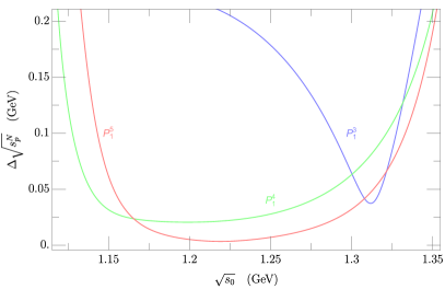
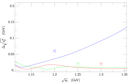
Figure 5: (Top panel) Global parameterizations systematic uncertainties, associated to the truncation of the single pole Padé sequence. (Bottom panel) The same uncertainties for a two pole Padé sequence.

Padé Approximants.– After defining the general $P^{N}_{M}$ Padé approximant in the previous subsection, Eq. (3), we now detail the particular sequences we use, their truncation, as well as how we determine their parameters and uncertainties from the dispersive output or the data parameterizations.

First of all, we choose $s_{0}$ in (3) to center the Taylor expansion defined in Eq. (4) in a point of the real axis near the resonance. The choice of Padé sequence, i.e., the $M$ in $P^{N}_{M}$, depends on the analytic structure of the function to be continued. For example, when studying a narrow, isolated resonance, setting $s_{0}$ near its mass ensures that there is a domain around $s_{0}$ where $F(s)$ is analytic but for the pole associated to that resonance. We can then set $M=1$ and thus approximate the amplitude by

$$P_{1}^{N}\left(s,s_{0}\right)=\sum_{k=0}^{N-1}a_{k}\left(s-s_{0}\right)^{k}+\frac{a_{N}\left(s-s_{0}\right)^{N}}{1-\frac{a_{N+1}}{a_{N}}\left(s-s_{0}\right)},$$ (16)

with $a_{n}=\frac{1}{n!}F^{(n)}\left(s_{0}\right)$ given by the derivatives of the function at $s_{0}$, as explained above. In this very simple case the pole and its residue are given by

$$s_{p}^{N}=s_{0}+\frac{a_{N}}{a_{N+1}},\quad Z^{N}=-\frac{\left(a_{N}\right)^{N+2}}{\left(a_{N+1}\right)^{N+1}}.$$ (17)

More often resonances lie close to other non-analytic structures like other poles or thresholds and their cuts. In such cases, we would choose a larger $M$, to mimic those additional singularities. In this work we have considered several possibilities ranging from $M=1$ to $M=3$. These additional poles, depending on the center, may crudely mimic the effect of the $f_{0}(980)$, the $f_{0}(1500)$, or any of the $K\bar{K}$, $\eta\eta$ or $\rho\rho$ thresholds. In Table 2 in the main text we have provided examples of results for $M=1,2$ and when both sequences converge, they give almost identical results.

Let us now turn to the calculation of uncertainties for a given center $s_{0}$. First we propagate the uncertainties in the amplitude in the real axis through the Padé coefficients to the pole, and this we call statistical uncertainties.

Systematic errors stem from truncating the Padé sequence to a given order $N$. Naively considering higher orders may approximate the amplitude better, but these require higher derivatives, which propagate larger statistical uncertainties. Given a fixed center $s_{0}$ and the poles extracted at order $N$ and $N-1$, we will estimate the systematic uncertainty associated to the truncation of the series as

$$\Delta\sqrt{s_{p}^{N}}=\left|\sqrt{s_{p}^{N}}-\sqrt{s_{p}^{N-1}}\right|,$$ (18)

which is shown for different centers in Fig. 5 using as input the “Global 1” parameterization. In the upper panel we show that, for the $P^{N}_{1}$ sequence, this uncertainty decreases as $N$ increases and that there is a plateau for the optimal choice of center around 1.2-1.25 GeV, reaching the $\sim 10\,$MeV level. In the lower panel we show a similar plot for the $P^{N}_{2}$ sequence, which seems to converge even faster and over a wider region. In view of these plots, we then decide to truncate the sequence when this systematic uncertainty becomes smaller than the statistical one. Then we choose our final $s_{0}$ as the one that minimizes the sum in quadrature of the statistical and systematic uncertainties.

Finally, there is an additional subtlety on how to determine the coefficients of each Padé approximant.

Padé approximants from derivatives.– These should be used only when we have an analytic formula for the parameterization and its derivatives, like in the “Global” case. This approach has been extensively used in the recent past with great success Masjuan and Sanz-Cillero (2013); Masjuan et al. (2014); Caprini et al. (2016); Peláez et al. (2017). Let us briefly summarize the main details here. As can be seen in Fig. 5 the $P^{N}_{M}$ Padé sequence for one or two poles seems to converge much better to the $f_{0}(1370)$ pole when $N>3$ and 2, respectively. The preferred center of the expansion lies around $1.2-1.25$ GeV for single-pole approximants, and above $1.35$ GeV for two-pole ones. Notice that already for $P^{4}_{1}$ and $P^{3}_{2}$ the systematic errors are small compared to the total error listed in Tab. 1. When using a two-pole Padé approximant we always find a second pole nearby. For $s_{0}$ values below roughly 1.2 GeV this second pole can be identified with the $f_{0}(980)$, whereas for centers above it seems to produce a narrow pole that can be associated to the $f_{0}(1500)$ resonance.

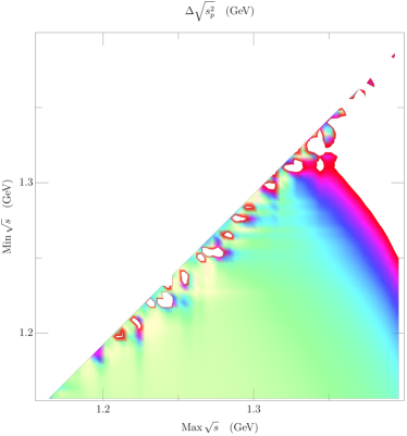
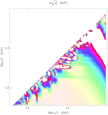
Figure 6: GKPY+Global Padé fit systematic uncertainties. We show the $P^{2}_{1}$ (left) and $P^{3}_{1}$ (right) systematic uncertainties associated to the selection the minimum and maximum values of $\sqrt{s}$ fitted. Notice how the $P^{3}_{1}$ fit produces a much smaller systematic uncertainty for a broad region.

Padé approximants fitted to the amplitudes.– Another possible approach is to perform a Padé fit to the amplitude of interest Ropertz et al. (2018). This is well suited when we do not know the analytic formula for the derivatives, like when using dispersion relations for the “Roy+CFD” or “Roy+Global” results. In this particular case the systematic spread is different. We no longer care about the center of the expansion $s_{0}$, but about the initial and final energy values to be fit. Thus, we will study a vast energy region and select the interval where our Padé sequence converges faster. Once again, we will consider the systematic uncertainty as the difference between the pole positions calculated at two consecutive orders, for the same fitted segment. For illustration, we show in Fig. 6 the systematic uncertainties for $P^{2}_{1},\,P^{3}_{1}$ when analytically continuing the Roy–Steiner equations output, with the Global1 parameterization as input. Two main features can be noticed, the first one is that $P^{3}_{1}$ produces on average a much smaller systematic uncertainty than $P^{2}_{1}$, and has a vast region for which it becomes negligible. The second is that this region includes segments of substantial length. Similar behavior is found when using the CFD parameterization. Both seem to favor segments with a length of roughly 0.15-0.2 GeV. Concerning the CFD parameterization, let us recall that it is piecewise in this region García-Martín et al. (2011b), and as such there will always be additional non-analytic structures nearby. Finally note that different sequence and methods produce different pole positions, although as seen in Table 2, they are compatible and overlap within uncertainties. This is a result of the sizable parameterization dependence that one always suffers when fitting data.

Unfortunately, this method does not produce a stable $f_{0}(1370)$ when using the forward dispersion relations. The main reason is that this amplitude dispersion relations include all partial waves with a given isospin combination, not only the scalar one. As a result, the $F^{00}$ includes and is actually dominated in this region by the $f_{2}(1270)$, which is narrower than our desired $f_{0}(1370)$. If one is to use a single-pole Padé, it will always find the $f_{2}(1270)$ as the dominant one. Including more poles in the denominator produces also a broader signal behind the tensor resonance. However, the spread of results is very large. We have found that using continued fractions, which in principle are not restricted regarding the number of poles they produce, is more suitable for this particular case.

.3 Forward Dispersion Relations for different isospin combinations

In the main text we have stated that the most precise Forward Dispersion Relation (FDR) to extract the isospin zero component is the one for the amplitude

$$F^{00}(s,0)\equiv(F^{0}(s,0)+2F^{2}(s,0))/3,$$ (19)

where $F^{I}(s,t)$ are the $\pi\pi$ scattering amplitudes with definite isospin $I$. Its small uncertainties are due to the positivity of all integrand contributions García-Martín et al. (2011b); Navarro Pérez et al. (2015). Other FDRs were also considered in these references, particularly the $F^{0+}=(F^{1}+F^{2})/3$, also with good positivity properties, and the $F^{I_{t}=1}$, which has the advantage of being dominated by the $\rho$ reggeon exchange at high energies, without the Pomeron contribution that dominates the other two.

Then, in Fig. 7, we show the difference between input and output for several FDRs and their uncertainty bands. In particular, one could consider extracting the pure $F^{0}$ component. In terms of the $F^{00}$, $F^{0+}$ and $F^{I_{t}=1}$ FDRs provided in García-Martín et al. (2011b); Navarro Pérez et al. (2015), this corresponds to $F^{0}=2F^{00}-F^{0+}+F^{I_{t}=1}$. We thus lose positivity in the integrands and the resulting uncertainty, shown in green, becomes larger than for $F^{00}$. The $F^{0+}$ does not contain isospin 0, but can be used to remove the $F^{1}$ contribution from $F^{I_{t}=1}$, thus avoiding the presence of yet another resonance pole in the region of interest (the $\rho(1450)$). The fulfillment of this FDR is plotted in Fig. 7 as a light red band, once again much larger than for $F^{00}$. Any other combination will thus suffer from the loss of positivity or the presence of the $F^{1}$ component and therefore a larger uncertainty than $F^{00}$, which is therefore the best choice for our calculations.

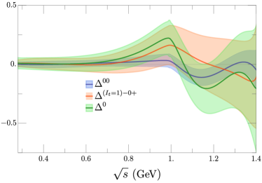
Figure 7: Differences between the the Input and FDR output for three different isospin combinations. The blue line corresponds to the difference for the $F^{00}$ amplitude, used in this work. The orange and green lines correspond to the $F^{I_{t}=1}-F^{0+}$ and $F^{0}$ amplitudes respectively. The colored bands represent the relatively uncertainties between Input and FDR output.

References

- Peláez (2016) J. R. Peláez, Phys.Rept. 658, 1 (2016), arXiv:1510.00653 [hep-ph] .
- Peláez and Rodas (2022) J. R. Peláez and A. Rodas, Phys. Rept. 969, 1 (2022), arXiv:2010.11222 [hep-ph] .
- Zyla et al. (2020) P. A. Zyla et al. (Particle Data Group), PTEP 2020, 083C01 (2020).
- Peláez et al. (2021) J. R. Peláez, A. Rodas, and J. Ruiz de Elvira, Eur. Phys. J. ST 230, 1539 (2021), arXiv:2101.06506 [hep-ph] .
- Caprini et al. (2006) I. Caprini, G. Colangelo, and H. Leutwyler, Phys.Rev.Lett. 96, 132001 (2006), arXiv:hep-ph/0512364 [hep-ph] .
- García-Martín et al. (2011a) R. García-Martín, R. Kaminski, J. R. Peláez, and J. Ruiz de Elvira, Phys.Rev.Lett. 107, 072001 (2011a), arXiv:1107.1635 [hep-ph] .
- Moussallam (2011) B. Moussallam, Eur. Phys. J. C71, 1814 (2011), arXiv:1110.6074 [hep-ph] .
- Descotes-Genon and Moussallam (2006) S. Descotes-Genon and B. Moussallam, Eur. Phys. J. C 48, 553 (2006), arXiv:hep-ph/0607133 .
- Peláez and Rodas (2020) J. Peláez and A. Rodas, Phys. Rev. Lett. 124, 172001 (2020), arXiv:2001.08153 [hep-ph] .
- Bugg (2007) D. Bugg, Eur. Phys. J. C 52, 55 (2007), arXiv:0706.1341 [hep-ex] .
- Klempt and Zaitsev (2007) E. Klempt and A. Zaitsev, Phys.Rept. 454, 1 (2007), arXiv:0708.4016 [hep-ph] .
- Ochs (2013) W. Ochs, J. Phys. G40, 043001 (2013), arXiv:1301.5183 [hep-ph] .
- Pawlicki et al. (1977) A. Pawlicki, D. Ayres, D. H. Cohen, R. Diebold, S. Kramer, and A. Wicklund, Phys. Rev. D 15, 3196 (1977).
- Cohen et al. (1980) D. H. Cohen, D. S. Ayres, R. Diebold, S. L. Kramer, A. J. Pawlicki, and A. B. Wicklund, Phys. Rev. D22, 2595 (1980).
- Etkin et al. (1982) A. Etkin et al., Phys. Rev. D25, 2446 (1982).
- Akesson et al. (1986) T. Akesson et al. (Axial Field Spectrometer), Nucl. Phys. B 264, 154 (1986).
- Gaspero (1993) M. Gaspero, Nucl. Phys. A 562, 407 (1993).
- Adamo et al. (1993) A. Adamo et al., Nucl. Phys. A 558, 13C (1993).
- Amsler et al. (1994) C. Amsler et al. (Crystal Barrel), Phys. Lett. B 322, 431 (1994).
- Amsler et al. (1992) C. Amsler et al. (Crystal Barrel), Phys. Lett. B 291, 347 (1992).
- Anisovich et al. (1994) V. Anisovich et al. (Crystal Ball), Phys. Lett. B 323, 233 (1994).
- Amsler et al. (1995a) C. Amsler et al. (Crystal Barrel), Phys. Lett. B 353, 571 (1995a).
- Amsler et al. (1995b) C. Amsler et al. (Crystal Barrel), Phys. Lett. B 342, 433 (1995b).
- Amsler et al. (1995c) C. Amsler et al. (Crystal Barrel), Phys. Lett. B 355, 425 (1995c).
- Abele et al. (1996a) A. Abele et al., Nucl. Phys. A 609, 562 (1996a), [Erratum: Nucl.Phys.A 625, 899–900 (1997)].
- Abele et al. (1996b) A. Abele et al. (Crystal Barrel), Phys. Lett. B 385, 425 (1996b).
- Barberis et al. (1999a) D. Barberis et al. (WA102), Phys. Lett. B 453, 305 (1999a), arXiv:hep-ex/9903042 .
- Barberis et al. (1999b) D. Barberis et al. (WA102), Phys. Lett. B 453, 325 (1999b), arXiv:hep-ex/9903044 .
- Bellazzini et al. (1999) R. Bellazzini et al. (GAMS), Phys. Lett. B 467, 296 (1999).
- Aitala et al. (2001a) E. Aitala et al. (E791), Phys. Rev. Lett. 86, 765 (2001a), arXiv:hep-ex/0007027 .
- Aitala et al. (2001b) E. Aitala et al. (E791), Phys. Rev. Lett. 86, 770 (2001b), arXiv:hep-ex/0007028 .
- Abele et al. (2001a) A. Abele et al. (Crystal Barrel), Eur. Phys. J. C 19, 667 (2001a).
- Abele et al. (2001b) A. Abele et al. (Crystal Barrel), Eur. Phys. J. C 21, 261 (2001b).
- Link et al. (2004) J. Link et al. (FOCUS), Phys. Lett. B 585, 200 (2004), arXiv:hep-ex/0312040 .
- Ablikim et al. (2005) M. Ablikim et al. (BES), Phys. Lett. B 607, 243 (2005), arXiv:hep-ex/0411001 [hep-ex] .
- Garmash et al. (2005) A. Garmash et al. (Belle), Phys. Rev. D 71, 092003 (2005), arXiv:hep-ex/0412066 .
- Cawlfield et al. (2006) C. Cawlfield et al. (CLEO), Phys. Rev. D 74, 031108 (2006), arXiv:hep-ex/0606045 .
- Bonvicini et al. (2007) G. Bonvicini et al. (CLEO), Phys. Rev. D 76, 012001 (2007), arXiv:0704.3954 [hep-ex] .
- Aaij et al. (2011) R. Aaij et al. (LHCb), Phys. Lett. B 698, 115 (2011), arXiv:1102.0206 [hep-ex] .
- d’Argent et al. (2017) P. d’Argent, N. Skidmore, J. Benton, J. Dalseno, E. Gersabeck, S. Harnew, P. Naik, C. Prouve, and J. Rademacker, JHEP 05, 143 (2017), arXiv:1703.08505 [hep-ex] .
- Hyams et al. (1973) B. Hyams et al., Nucl. Phys. B64, 134 (1973).
- Grayer et al. (1974) G. Grayer et al., Nucl. Phys. B75, 189 (1974).
- Hyams et al. (1975) B. Hyams et al., Nucl. Phys. B100, 205 (1975).
- Estabrooks (1979) P. Estabrooks, Phys. Rev. D 19, 2678 (1979).
- Sarantsev et al. (2021) A. V. Sarantsev, I. Denisenko, U. Thoma, and E. Klempt, Phys. Lett. B 816, 136227 (2021), arXiv:2103.09680 [hep-ph] .
- Albaladejo and Oller (2008) M. Albaladejo and J. A. Oller, Phys. Rev. Lett. 101, 252002 (2008), arXiv:0801.4929 [hep-ph] .
- Guo et al. (2012a) Z.-H. Guo, J. A. Oller, and J. Ruiz de Elvira, Phys. Rev. D86, 054006 (2012a), arXiv:1206.4163 [hep-ph] .
- Guo et al. (2012b) Z.-H. Guo, J. A. Oller, and J. Ruiz de Elvira, Phys. Lett. B 712, 407 (2012b), arXiv:1203.4381 [hep-ph] .
- Ledwig et al. (2014) T. Ledwig, J. Nieves, A. Pich, E. Ruiz Arriola, and J. Ruiz de Elvira, Phys. Rev. D 90, 114020 (2014), arXiv:1407.3750 [hep-ph] .
- Ropertz et al. (2018) S. Ropertz, C. Hanhart, and B. Kubis, Eur. Phys. J. C78, 1000 (2018), arXiv:1809.06867 [hep-ph] .
- Rodas et al. (2022) A. Rodas, A. Pilloni, M. Albaladejo, C. Fernandez-Ramirez, V. Mathieu, and A. P. Szczepaniak (Joint Physics Analysis Center), Eur. Phys. J. C 82, 80 (2022), arXiv:2110.00027 [hep-ph] .
- García-Martín et al. (2011b) R. García-Martín, R. Kamiński, J. R. Peláez, J. Ruiz de Elvira, and F. J. Ynduráin, Phys.Rev. D83, 074004 (2011b), arXiv:1102.2183 [hep-ph] .
- Pelaez and Rodas (2018) J. R. Pelaez and A. Rodas, Eur. Phys. J. C78, 897 (2018), arXiv:1807.04543 [hep-ph] .
- Pelaez and Yndurain (2005) J. R. Pelaez and F. J. Yndurain, Phys. Rev. D71, 074016 (2005), arXiv:hep-ph/0411334 [hep-ph] .
- Kaminski et al. (2008) R. Kaminski, J. R. Pelaez, and F. J. Yndurain, Phys. Rev. D77, 054015 (2008), arXiv:0710.1150 [hep-ph] .
- Navarro Pérez et al. (2015) R. Navarro Pérez, E. Ruiz Arriola, and J. Ruiz de Elvira, Phys. Rev. D 91, 074014 (2015), arXiv:1502.03361 [hep-ph] .
- Roy (1971) S. M. Roy, Phys.Lett. 36B, 353 (1971).
- Yndurain et al. (2007) F. J. Yndurain, R. Garcia-Martin, and J. R. Pelaez, Phys. Rev. D76, 074034 (2007), arXiv:hep-ph/0701025 [hep-ph] .
- Caprini (2008) I. Caprini, Phys. Rev. D77, 114019 (2008), arXiv:0804.3504 [hep-ph] .
- Švarc et al. (2013) A. Švarc, M. Hadzimehmedovic, H. Osmanovic, J. Stahov, L. Tiator, and R. L. Workman, Phys. Rev. C88, 035206 (2013), arXiv:1307.4613 [hep-ph] .
- Švarc et al. (2014) A. Švarc, M. Hadžimehmedović, H. Osmanović, J. Stahov, L. Tiator, and R. L. Workman, Phys. Rev. C89, 065208 (2014), arXiv:1404.1544 [nucl-th] .
- Švarc et al. (2015) A. Švarc, M. Hadžimehmedović, H. Osmanović, J. Stahov, and R. L. Workman, Phys.Rev. C91, 015207 (2015), arXiv:1405.6474 [nucl-th] .
- Masjuan and Sanz-Cillero (2013) P. Masjuan and J. J. Sanz-Cillero, Eur. Phys. J. C73, 2594 (2013), arXiv:1306.6308 [hep-ph] .
- Masjuan et al. (2014) P. Masjuan, J. Ruiz de Elvira, and J. J. Sanz-Cillero, Phys. Rev. D90, 097901 (2014), arXiv:1410.2397 [hep-ph] .
- Caprini et al. (2016) I. Caprini, P. Masjuan, J. Ruiz de Elvira, and J. J. Sanz-Cillero, Phys. Rev. D93, 076004 (2016), arXiv:1602.02062 [hep-ph] .
- Peláez et al. (2017) J. R. Peláez, A. Rodas, and J. Ruiz de Elvira, Eur. Phys. J. C77, 91 (2017), arXiv:1612.07966 [hep-ph] .
- Schlessinger (1968) L. Schlessinger, Phys. Rev. 167, 1411 (1968).
- Tripolt et al. (2017) R.-A. Tripolt, I. Haritan, J. Wambach, and N. Moiseyev, Phys. Lett. B 774, 411 (2017), arXiv:1610.03252 [hep-ph] .
- Binosi and Tripolt (2020) D. Binosi and R.-A. Tripolt, Phys. Lett. B 801, 135171 (2020), arXiv:1904.08172 [hep-ph] .
- Binosi et al. (2022) D. Binosi, A. Pilloni, and R.-A. Tripolt, (2022), arXiv:2205.02690 [hep-ph] .
- Pelaez et al. (2019) J. Pelaez, A. Rodas, and J. Ruiz de Elvira, Eur. Phys. J. C 79, 1008 (2019), arXiv:1907.13162 [hep-ph] .
- Abele et al. (1996c) A. Abele et al. (Crystal Barrel), Phys. Lett. B 385, 425 (1996c).
- Albrecht et al. (2020) M. Albrecht et al. (Crystal Barrel), Eur. Phys. J. C 80, 453 (2020), arXiv:1909.07091 [hep-ex] .
- Amsler et al. (1995d) C. Amsler et al. (Crystal Barrel), Phys. Lett. B 355, 425 (1995d).
- Anisovich and Sarantsev (2009) V. V. Anisovich and A. V. Sarantsev, Int. J. Mod. Phys. A 24, 2481 (2009).
- Au et al. (1987) K. L. Au, D. Morgan, and M. R. Pennington, Phys. Rev. D35, 1633 (1987).
- Barberis et al. (2000) D. Barberis et al. (WA102), Phys. Lett. B 471, 440 (2000), arXiv:hep-ex/9912005 .
- Bargiotti et al. (2003) M. Bargiotti et al. (OBELIX), Eur. Phys. J. C 26, 371 (2003).
- Bertin et al. (1997) A. Bertin et al. (OBELIX), Phys. Lett. B 408, 476 (1997).
- Bugg et al. (1996) D. V. Bugg, B. S. Zou, and A. V. Sarantsev, Nucl. Phys. B471, 59 (1996).
- Janssen et al. (1995) G. Janssen, B. C. Pearce, K. Holinde, and J. Speth, Phys. Rev. D52, 2690 (1995), arXiv:nucl-th/9411021 [nucl-th] .
- Kaminski et al. (1999) R. Kaminski, L. Lesniak, and B. Loiseau, Eur. Phys. J. C 9, 141 (1999), arXiv:hep-ph/9810386 .
- Tornqvist (1995) N. A. Tornqvist, Z. Phys. C68, 647 (1995), arXiv:hep-ph/9504372 [hep-ph] .
- Ananthanarayan et al. (2001) B. Ananthanarayan, G. Colangelo, J. Gasser, and H. Leutwyler, Phys.Rept. 353, 207 (2001), arXiv:hep-ph/0005297 [hep-ph] .
- Buettiker et al. (2004) P. Buettiker, S. Descotes-Genon, and B. Moussallam, Eur. Phys. J. C33, 409 (2004), arXiv:hep-ph/0310283 [hep-ph] .
- Hoferichter et al. (2016) M. Hoferichter, J. Ruiz de Elvira, B. Kubis, and U.-G. Meißner, Phys. Rept. 625, 1 (2016), arXiv:1510.06039 [hep-ph] .
- de Montessus de Ballore (1902) R. de Montessus de Ballore, Bull. Soc. Math. France 30, 28 (1902).
- Gribov and Pomeranchuk (1962) V. N. Gribov and I. Ya. Pomeranchuk, Sov.Phys.JETP 15, 788L (1962), [Phys. Rev. Lett.8,343(1962)].
- Pelaez and Yndurain (2004) J. R. Pelaez and F. J. Yndurain, Phys. Rev. D69, 114001 (2004), arXiv:hep-ph/0312187 [hep-ph] .