Strong Lensing Source Reconstruction Using Continuous Neural Fields

Abstract

From the nature of dark matter to the rate of expansion of our Universe, observations of distant galaxies distorted through strong gravitational lensing have the potential to answer some of the major open questions in astrophysics. Modeling galaxy-galaxy strong lensing observations presents a number of challenges as the exact configuration of both the background source and foreground lens galaxy is unknown. A timely call, prompted by a number of upcoming surveys anticipating high-resolution lensing images, demands methods that can efficiently model lenses at their full complexity. In this work, we introduce a method that uses continuous neural fields to non-parametrically reconstruct the complex morphology of a source galaxy while simultaneously inferring a distribution over foreground lens galaxy configurations. We demonstrate the efficacy of our method through experiments on simulated data targeting high-resolution lensing images similar to those anticipated in near-future astrophysical surveys.

MIT-CTP/5444

1 Introduction

According to general relativity, the warping of space-time in the vicinity of a massive celestial body can distort the path of light rays traversing close-by. This phenomenon, called gravitational lensing (Einstein, 1936), is a powerful probe of the distribution of structures in our Universe. In the strong lensing regime, multiple highly magnified images of background luminous sources can be observed. This is a versatile astrophysical laboratory that has been used to characterize distant galaxies (Wuyts et al., 2012; Yuan et al., 2017), constrain the abundance of dark matter substructures (Dalal & Kochanek, 2002; Vegetti et al., 2014; Hezaveh et al., 2016; Gilman et al., 2019; Hsueh et al., 2020; Şengül et al., 2021; Meneghetti et al., 2020), and provide percent-level estimates of the expansion rate of the Universe (Birrer et al., 2020).

A particular challenge with fully exploiting observations of galaxy-galaxy strong gravitational lenses — where an extended background source is lensed by a foreground galaxy — is that of accounting for the complex morphologies of lensed galaxies. Although sources in low-resolution images can be adequately modeled using phenomenological parameterizations such as one or several Sérsic profiles (Sérsic, 1963), this approach is inadequate for modeling higher-fidelity lensing observations such as those from ongoing, upcoming, and proposed telescopes like the Hubble Space Telescope (HST), JWST, Euclid, and the Extremely Large Telescope (ELT). The development of new methods is especially timely, given the large number of high-resolution lenses that are expected to be imaged by next-generation cosmological surveys (Collett, 2015) and their potential to weigh in on the nature of dark matter (Simon et al., 2019).

A number of methods have been proposed that go beyond using simple parameterization for the background galaxies. They include regularized semi-linear inversion (Warren & Dye, 2003), the use of truncated bases like shapelets (Birrer et al., 2015; Birrer & Amara, 2018) or wavelets (Galan et al., 2021), and the use of adaptive source-plane pixelizations (Vegetti & Koopmans, 2009; Nightingale et al., 2018). More recently, deep learning techniques, for example variational autoencoders (Chianese et al., 2020), recurrent inference machines (Morningstar et al., 2019), and Gaussian process-inspired inference (Karchev et al., 2022) have also shown promise. Downstream analyses often benefit from, and sometimes require, a probabilistic treatment of both the source and lens. Using variational methods, Karchev et al. 2022 demonstrated the ability to recover the posterior distribution over both the lens parameter and a complex source configuration.

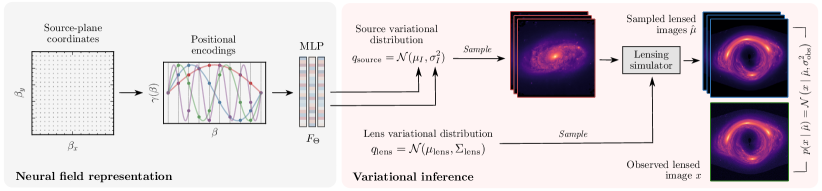
Figure 1: A schematic overview of the method used in this work.

In this paper, we explore a complementary approach for probabilistic reconstruction of complex morphologies of strongly lensed galaxies from high-resolution images while simultaneously recovering the lens mass distribution. Our key contribution is to treat the source-light distribution as a continuous neural field, optimized using gradient-based variational inference. Together with recovering a posterior distribution over the lens model parameters, our approach is able to infer high-resolution images of the source galaxy in its full complexity. In the context of strong lensing, neural fields have previously been proposed for modeling the density profile of the smooth lens galaxy (Biggio et al., 2021).

2 Methodology

Our proposal takes the “analysis by synthesis” approach to conduct probabilistic inference on both the source image and the lens configuration using a differentiable lensing model. We describe the three key components of this generative pipeline below: (1) the differentiable lensing model used for rendering and the relevant strong-lensing physics, (2) the continuous neural representation of the source, and (3) the variational inference procedure used to simultaneously infer the lens parameter and source posteriors.

2.1 Strong Lensing and the Synthesis Model

At the heart of our approach is a differentiable renderer that takes the source and lens configurations, and outputs modeled lensing observations. The simulator we use is a modified version of gigalens (Gu et al., 2022), written in Jax (Bradbury et al., 2018).

The position of the source in the lens plane $\theta$ can be evaluated using the lens equation, $\beta=\theta-\phi(\theta)$. Here $\beta$ is the position in the source plane and $\phi(\theta)$ is the deflection vector, given by the gradient of the projected gravitational potential $\psi_{\mathrm{G}}(\theta)$ of the lens, $\phi(\theta)=\nabla\psi_{\mathrm{G}}(\theta)$. The lens equation relates the lens-plane coordinates back to those in the source-plane. Given an extended source light profile $f_{\mathrm{s}}$ and a lensing mass distribution, we can reconstruct the lens-plane observation $f_{\mathrm{s}}^{\prime}$ by evaluating the source light on the lens plane, $f_{\mathrm{s}}^{\prime}({\theta})=f_{\mathrm{s}}({\theta}-{\phi}({\theta}))$. We refer to, e.g., Treu (2010) for additional details of the strong lensing formalism.

The main lens deflector is modeled using the commonly employed Singular Isothermal Ellipsoid (SIE) parameterization (Kormann et al., 1994; Treu, 2010). The deflection vector field in this case is given in terms of angular coordinates $\theta_{x}$ and $\theta_{y}$ via (see e.g.,  Keeton 2001)

$$\phi_{\mathrm{lens},x}=\frac{\theta_{\mathrm{E}}q}{\sqrt{1-q^{2}}}\tan^{-1}\left[\frac{\sqrt{1-q^{2}}\theta_{x}}{\chi}\right]$$ (1)

$$\phi_{\mathrm{lens},y}=\frac{\theta_{\mathrm{E}}q}{\sqrt{1-q^{2}}}\tanh^{-1}\left[\frac{\sqrt{1-q^{2}}\theta_{y}}{\chi+q^{2}}\right],$$

where $q$ is the axis ratio ($q=1$ corresponding to a spherical lens), $\chi\equiv\sqrt{\theta_{x}^{2}q^{2}+\theta_{y}^{2}}$, and $\theta_{\mathrm{E}}$ is the Einstein radius denoting the characteristic lensing scale.

The lens orientation is specified in terms of eccentricities $\left(\epsilon_{1},\epsilon_{2}\right)=\frac{1-q}{1+q}\left(\cos(2\psi),\sin(2\psi)\right)$, where $\psi$ is a rotation angle. The large-scale lensing effect of the local environment is included through an external shear component $\{\gamma_{1},\gamma_{2}\}$ with deflection vector $\left(\phi_{\mathrm{ext},x},\phi_{\mathrm{ext},y}\right)=\left(\gamma_{1}\theta_{x}+\gamma_{2}\theta_{y},\gamma_{2}\theta_{x}-\gamma_{1}\theta_{y}\right)$.

After allowing for an overall offset $\left(\theta_{x,0},\theta_{y,0}\right)$ between the lens and source center lines of sight, our lens mass model consists of 7 parameters $\{\theta_{\mathrm{E}},\theta_{x,0},\theta_{y,0},\epsilon_{1},\epsilon_{2},\gamma_{1},\gamma_{2}\}$. We include the full list of lens model parameters and their assumed prior distributions in Tab. 1.

Table 1: List of parameters used in the lens model and their corresponding assumed prior distributions.

Parameter	Symbol	Prior
Einstein radius	$\theta_{\mathrm{E}}$	$\mathcal{U}(1^{\prime\prime},2^{\prime\prime})$
Source-lens offset	$\theta_{x,0},\theta_{y,0}$	$\mathcal{U}(-0.5^{\prime\prime},0.5^{\prime\prime})$
Eccentricities	$\epsilon_{1},\epsilon_{2}$	$\mathcal{N}(0,0.3)$
External shear	$\gamma_{1},\gamma_{2}$	$\mathcal{N}(0,0.05)$

2.2 Continuous Neural Representation of the Source

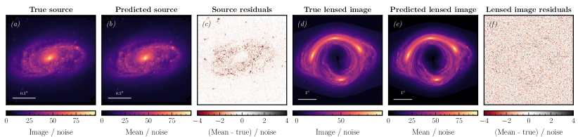
Figure 2: Results of reconstructing the source through our coordinate-based neural network pipeline using a mock lensed image of galaxy NGC2906. The (a) true source, (b) reconstructed source mean, (c) reconstructed mean minus true source residuals, (d) true lensed image, (e) reconstructed lensed image, and (f) reconstructed mean minus true lensed image residuals are shown. All images are normalized by the observation noise.

In our framework, the source-light distribution is modeled using a continuous neural field $F_{\Theta}:\mathbb{R}^{2}\mapsto\mathbb{R}^{2}$, which takes the source-plane coordinates $\{\beta_{x},\beta_{y}\}$ in $\mathbb{R}^{2}$ as input and outputs the mean and variance of the light intensity, modeled as a Gaussian distribution $I({x,y})\sim\mathcal{N}\left(\mu_{I}({x,y}),\sigma^{2}_{I}({x,y})\right)$.

Based on the universal function approximation theorem (Hornik et al., 1989), a naïve choice is to parameterize $F_{\Theta}$ as a vanilla neural network. Although the theorem guarantees the existence of good approximations, it makes no claims of how easy or difficult it would be to attain them. Empirical analyses uncovered an intrinsic learning bias for standard network architectures to favor fitting simpler, low-spatial frequency components of the target function under gradient descent (Zhang et al., 2021; Arpit et al., 2017; Ulyanov et al., 2018; Rahaman et al., 2019). Using new tools such as the neural tangent kernel (NTK, Jacot et al. 2018), recent progress in deep learning theory describe this phenomena as a “spectral bias” that slows down convergence over high-frequency components of the target function exponentially, which often result in poorly-fit models (Rahaman et al., 2019; Cao et al., 2019).

This problem can be addressed by adding positional encodings, now ubiquitously used in natural language processing (Gehring et al., 2017; Vaswani et al., 2017; Devlin et al., 2018). For an input $\beta\in\mathbb{R}$, positional encodings lift the input coordinates $\beta$ into a higher-dimensional spectral domain with $2\times L_{\mathrm{max}}$ dimensions per input dimension:

$$\begin{split}\gamma(\beta)=\big{[}&\sin(\beta),\cos(\beta),\sin(2\beta),\cos(2\beta),\ldots\\ &\sin\left(2^{L_{\mathrm{max}}-1}\beta\right),\cos\left(2^{L_{\mathrm{max}}-1}\beta\right)\big{]}^{\mathrm{T}},\end{split}$$ (2)

where $L_{\mathrm{max}}$ is the maximum bandwidth of the encoding. When applied to low-dimensional spaces such as image coordinates, such a scheme synthesizes high-fidelity reconstructions (Mildenhall et al., 2020), and was most recently applied in the astrophysics domain for tomographic reconstruction of lensed black hole emission in interferometric observations Levis et al. (2022). We implement $F_{\Theta}$ as a four-layer multi-layer perceptron (MLP) with ReLU activations and hidden dimension $256$. The intrinsic modeling bias of such networks is described in detail in (Tancik et al., 2020).

Higher values of the bandwidth hyperparameter $L_{\mathrm{max}}$ encourage reconstructing higher-frequency features, but may lead to overfitting on noise. We found $L_{\mathrm{max}}=5$ to work well in our set-up. Alternative schemes for lifting the input coordinates such as random Fourier features may be advantageous (Rahimi & Recht, 2008), and we discuss these in Sec. 4 and in App. A.

2.3 Variational Inference

We use variational inference (Jordan et al., 1999; Blei et al., 2017) to simultaneously fit for the joint distribution of the $n_{\mathrm{lens}}=7$ lens parameters alongside the source intensity distribution on a specified grid on the source plane. The variational ansatz on the lens parameters is taken to be a multivariate Normal distribution $q_{\mathrm{lens}}=\mathcal{N}(\mu_{\mathrm{lens}},\Sigma_{\mathrm{lens}})$, where $\mu_{\mathrm{lens}}$ is the mean vector and $\Sigma_{\mathrm{lens}}$ the parameter covariance matrix. We fit for the $n_{\mathrm{lens}}(n_{\mathrm{lens}}+1)/2$-parameter lower-triangular Cholesky factor $L$ of the covariance matrix, $\Sigma_{\mathrm{lens}}\equiv LL^{T}$, ensuring positivity of the diagonal component through the projection $\operatorname{Softplus}(\cdot)\equiv\log\left(1+e^{(\cdot)}\right)$.

The source on the other hand is modeled using a diagonal Normal distribution $q_{\mathrm{source}}=\mathcal{N}(\mu_{I},\sigma_{I}^{2})$, with the means and variances evaluated on the source grid as the outputs of the neural network $F_{\Theta}$. In this proof-of-principle exposition we do not model correlations between the lens and source parameters, leaving their inclusion to future work. In the following, the lens and source parameters (SIE parameters and intensities on a grid, respectively) are jointly denoted by $\vartheta$.

Given a pixelized lensed image $x$, the source and lens variational distributions, parameterized by $\phi$ and jointly denoted $q_{\phi}(\vartheta)$, are obtained by minimizing the reverse KL-divergence between the true and variational posterior distributions, $D_{\mathrm{KL}}\left(q_{\phi}\mid\mid p(\vartheta\mid x)\right)$. This is done by maximizing the model log-evidence $\log p(x)$ or, in practice using the tractable evidence lower bound (ELBO),

$$\operatorname{ELBO}\equiv\mathbb{E}_{\vartheta\sim q_{\phi}(\vartheta)}\left[\log p(x,\vartheta)-\log q_{\phi}(\vartheta)\right],$$ (3)

as the optimization objective since $\log p(x)-\operatorname{ELBO}=D_{\mathrm{KL}}\left(q_{\phi}\mid\mid p(\vartheta\mid x)\right)$. The expectation in the ELBO is taken through Monte Carlo sampling from the source and lens variational distributions at each optimization step. ELBO gradients are straightforwardly computed using the reparameterization trick (Kingma & Welling, 2013) since all the distributions employed are reparameterizable. We emphasize that the model only has access to the lensed image $x$ and not the ground-truth source.

Monte Carlo samples from the lens and source distribution are passed through the differentiable lensing pipeling to produce lensed image samples $\{\hat{\mu}(\vartheta)\}$. The joint likelihood $p(x,\vartheta)=p(x\mid\vartheta)\,p(\vartheta)$ is evaluated by combining the prior with the data likelihood, modeled as Normal; $p(x\mid\vartheta)=\mathcal{N}\left(x\mid\hat{\mu}(\vartheta),\sigma_{\mathrm{obs}}^{2}\right)$. Priors on the lens parameters are shown in Tab. 1.

The variational parameters—the weights and biases of $F_{\Theta}$ in the case of the source, and the mean and lower-triangular Cholesky matrix elements for the lens—are optimized using the AdamW optimizer (Kingma & Ba, 2014; Loshchilov & Hutter, 2017) over 15,000 steps. The learning rate is increased from zero to $10^{-3}$ over 2000 steps, then decreased via cosine annealing over the course of optimization. Fitting a lensed image typically takes $\sim 20$ minutes on a single Nvidia V100 GPU. The pipeline is constructed using the neural network and optimization libraries Flax (Heek et al., 2020) and Optax (Hessel et al., 2020).

A schematic illustration of the high-level features of the method are shown in Fig. 1.

3 Experiments

We test our source and lens reconstruction pipeline using an image of galaxy NGC2906 imaged by the Hubble Space Telescope as the mock source. A lensed image of size $500\times 500$ pixels is generated with image side 5 arcmin, corresponding to pixel size of 10 mas. A Gaussian point-spread function kernel is included with FWHM of 5 mas (Simon et al., 2019), although it has minimal effect given the pixel scale. Uniform Gaussian noise is added to the pixels such that the mean signal-to-noise ratio around the lensed ring (defined as pixels that are at least 50% as bright as the brightest pixel) is $\mathrm{SNR}\sim 60$. The lens parameters used to simulate the mock image are chosen as $\{\theta_{\mathrm{E}},\theta_{x,0},\theta_{y,0},\epsilon_{1},\epsilon_{2},\gamma_{1},\gamma_{2}\}=\{1.3^{\prime\prime},0.1^{\prime\prime},0.0^{\prime\prime},0.2,0.1,-0.02,0.02\}$.

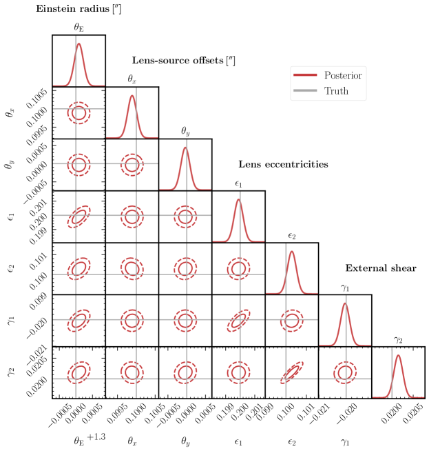
Figure 3: Individual and joint marginal posteriors on the SIE lens galaxy and external shear parameters obtained in our experiment. The ellipses show the 1- and 2-$\sigma$ containment of the joint posteriors. True parameter points from which the lensed image was simulated are indicated with grey lines. Faithful recovery of the true parameters is seen.

The results of our source and lensed image reconstruction are shown in Fig. 2, with all results normalized to the standard deviation of observation noise. The reconstructed source (b) is seen to provide a visually good representation of the unlensed galaxy (a). The reconstructed lensed image (e) again faithfully reproduces the observed lensed image (d), additionally corroborated by the normalized residuals (f). Some significant residual structures in the source plane are observed in (c); this can at least partially be attributed to a simplistic choice of source pixelization, discussed below. Example reconstructions for additional mock source and lens configurations are presented in App. B.

Figure 3 shows the 1-D and 2-D joint marginal posteriors inferred for the lens and external shear parameters in our experiment. 1-D marginals are shown as Gaussian profiles, while the 2-D joint distributions are represented through their 1- and 2-$\sigma$ containment regions. The true simulated parameters are indicated with grey lines. Successful recovery of the lens parameters within modeled uncertainty is seen in all cases.

4 Discussion and Future Work

In this ongoing work, we have explored the use of continuous neural fields for modeling morphologically complex gravitationally lensed galaxies. Our method is able to provide a probabilistic reconstruction of lensed galaxies with complex small-scale structure within minutes of wall-clock time, while simultaneously inferring a posterior over the parameterized macroscopic lens deflector field. Although our results are encouraging, practical deployment of the method will require several extensions and modifications to the framework. We conclude by discussing these extensions alongside caveats associated with the proposed method.

In our method, the prior over the source reconstruction is implicit, and it occurs through two separate mechanisms. First, it is affected by the bandwidth limit used in the positional encoding. Second, a low-frequency bias occurs through early stopping of the optimization process, which prevents the neural network from fitting higher-frequency features and overfitting on noise. Although the dynamics associated with with this phenomenon have been well-studied (Roberts et al., 2022), a dedicated understanding in the context of our specific domain could inform more principled regularization for a given lens observation configuration. Empirically, we found that excessive optimization leads to overfitting on noisy images, which in turn can produce systematic biases in the reconstruction of lens galaxy parameters.

The positional encoding used in this paper is non-isotropic under rotation, because it processes the two axes independently from each other. An isotropic alternative is random Fourier features (RFF, see Rahimi & Recht (2008)), which samples a projection matrix from an isotropic distribution such as a multivariate Gaussian (Yang et al., 2022). Random Fourier features treat the input coordinates as full vectors during the spectral projection. The downside is due to its statistical nature, RFF require a larger number of features. The cut-off band-limit of both encodings can be controlled explicitly through the spectral mixture used to lift the input. In a learned variant of RFF, called the learned Fourier features, these weights are updated through gradient descent. This means more careful regularization of the cut-off bandwidth of the projection matrix is needed.

Modifications to the lensing pipeline can further improve the quality and robustness of reconstruction. For example, the current implementation glosses over subtleties associated with the source-plane pixelization. Instead, it models the pixelated data in the lens plane through individual points in the source plane. In addition, representing the source plane with the same resolution as the lens plane has been shown to be sub-optimal given the coordinate distortion inherent to the lensing process (Warren & Dye, 2003); the contribution of source-plane regions corresponding to larger magnification should be evaluated at a relatively finer resolution. Our continuous, rather than discretely-sampled, representation of the source should make our framework amenable to a more principled treatment of the the source-plane pixelization.

Finally, it is possibly to use more expressive variational distributions beyond the Gaussian ansatz and explicitly model covariances between the source galaxy and lens parameters. This could be accomplished, for example, by modeling the lens parameters using a normalizing flow conditioned on summary features extracted from the reconstructed source over the course of optimization. Having demonstrated the potential of the method in a proof-of-principle setting, we leave these extensions to future work.

Software and Data

Code for reproducing the results presented in this paper is available at https://github.com/smsharma/lensing-neural-fields. This research made use of the Astropy (Astropy Collaboration, 2013, 2018, 2022), Flax (Heek et al., 2020), gigalens (Gu et al., 2022), IPython (Pérez & Granger, 2007), Jax (Bradbury et al., 2018; Babuschkin et al., 2020), jaxinterp2d (Coogan, ), Jupyter (Kluyver et al., 2016), lenstronomy (Birrer & Amara, 2018; Birrer et al., 2021), Matplotlib (Hunter, 2007), NumPy (Harris et al., 2020), numpyro (Phan et al., 2019), Optax (Hessel et al., 2020), scikit-image (van der Walt et al., 2014), and SciPy (Virtanen et al., 2020) software packages.

Appendix A Role of positional encodings

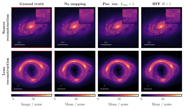
Figure 4: Source (top row) and lens (bottom row) reconstruction using variations on mapping the input coordinates to a higher-dimensional feature space. The ground truth (first column), no coordinate mapping (second column), positional encodings (third column; baseline), and Gaussian random Fourier features (last column) are shown. Poor reconstruction of small-scale source galaxy features is seen when not employing an input mapping.

Mapping the input source coordinates into a specific higher-dimensional feature space encourages effective reconstruction of small-scale (high-frequency) features in the source galaxy. This is demonstrated in Fig. 4, where we show the baseline reconstructed source along with a zoom-in inset (top row) and lens (bottom row) for various mapping configurations. The ground truths (first column), results with no coordinate mappings (second column), and standard sinusoidal positional encodings (Eq. (2) with bandwidth hyperparameter set to $L_{\mathrm{max}}=5$; third column) are shown. It can be seen that small-scale galaxy features are better reconstructed when using positional encodings, whereas these appear washed out without the additional encoding step.

Additionally, we show results using a Gaussian random Fourier feature mapping (Tancik et al., 2020; Rahimi & Recht, 2007; Yang et al., 2022). Here, the source coordinates $\beta$ are lifted through the mapping $\mathrm{RFF}(\beta)_{i}=\sin(w_{ij}\beta_{j}+b_{i})$ where the weights and biases are drawn as $w_{ij}\sim\mathcal{N}\left(0,(B/2)^{2}\right)$ and $b_{i}\sim\mathcal{U}(-1,1)$ at initialization. The last column of Fig. 4 shows results when using this mapping, setting the bandwidth hyperparameter $B=5$. Similar performance in reconstructing small-scale galaxy features to that obtained using the standard positional encoding scheme can be seen in this case.

Appendix B Additional examples

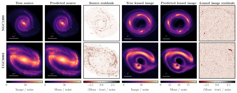
Figure 5: Reconstruction results using additional source and lens configurations, in the same format as Fig. 2.

In Fig. 5 we show additional source reconstruction results on mock images simulated using images of galaxies NGC1300 and UGC6309 taken by Hubble. The same lens configuration as in the baseline example is used in the first case, while in the second case we set $\{\theta_{\mathrm{E}},\theta_{x,0},\theta_{y,0},\epsilon_{1},\epsilon_{2},\gamma_{1},\gamma_{2}\}=\{1.1^{\prime\prime},0.4^{\prime\prime},-0.1^{\prime\prime},0.1,0.15,-0.03,0.04\}$.

References

- Arpit et al. (2017) Arpit, D., Jastrzebski, S., Ballas, N., Krueger, D., Bengio, E., Kanwal, M. S., Maharaj, T., Fischer, A., Courville, A., Bengio, Y., et al. A closer look at memorization in deep networks. In International conference on machine learning, pp. 233–242. PMLR, 2017.
- Astropy Collaboration (2013) Astropy Collaboration. Astropy: A community Python package for astronomy. Astronomy & Astrophysics, 558:A33, October 2013. doi: 10.1051/0004-6361/201322068.
- Astropy Collaboration (2018) Astropy Collaboration. The Astropy Project: Building an Open-science Project and Status of the v2.0 Core Package. The Astronomical Journal, 156(3):123, September 2018. doi: 10.3847/1538-3881/aabc4f.
- Astropy Collaboration (2022) Astropy Collaboration. The Astropy Project: Sustaining and Growing a Community-oriented Open-source Project and the Latest Major Release (v5.0) of the Core Package. The Astrophysical Journal, 935(2):167, August 2022. doi: 10.3847/1538-4357/ac7c74.
- Babuschkin et al. (2020) Babuschkin, I., Baumli, K., Bell, A., Bhupatiraju, S., Bruce, J., Buchlovsky, P., Budden, D., Cai, T., Clark, A., Danihelka, I., Fantacci, C., Godwin, J., Jones, C., Hennigan, T., Hessel, M., Kapturowski, S., Keck, T., Kemaev, I., King, M., Martens, L., Mikulik, V., Norman, T., Quan, J., Papamakarios, G., Ring, R., Ruiz, F., Sanchez, A., Schneider, R., Sezener, E., Spencer, S., Srinivasan, S., Stokowiec, W., and Viola, F. The DeepMind JAX Ecosystem, 2020. URL http://github.com/deepmind.
- Biggio et al. (2021) Biggio, L., Galan, A., Peel, A., Vernardos, G., and Courbin, F. Differentiable Strong Lensing for Complex Lens Modelling. In Machine Learning and the Physical Sciences Workshop at the 35th Conference on Neural Information Processing Systems (NeurIPS), 2021.
- Birrer & Amara (2018) Birrer, S. and Amara, A. lenstronomy: Multi-purpose gravitational lens modelling software package. Physics of the Dark Universe, 22:189–201, 2018.
- Birrer et al. (2015) Birrer, S., Amara, A., and Refregier, A. Gravitational lens modeling with basis sets. The Astrophysical Journal, 813(2):102, 2015.
- Birrer et al. (2020) Birrer, S., Shajib, A., Galan, A., Millon, M., Treu, T., Agnello, A., Auger, M., Chen, G.-F., Christensen, L., Collett, T., et al. Tdcosmo-iv. hierarchical time-delay cosmography–joint inference of the hubble constant and galaxy density profiles. Astronomy & Astrophysics, 643:A165, 2020.
- Birrer et al. (2021) Birrer, S., Shajib, A. J., Gilman, D., Galan, A., Aalbers, J., Millon, M., Morgan, R., Pagano, G., Park, J. W., Teodori, L., Tessore, N., Ueland, M., de Vyvere, L. V., Wagner-Carena, S., Wempe, E., Yang, L., Ding, X., Schmidt, T., Sluse, D., Zhang, M., and Amara, A. lenstronomy ii: A gravitational lensing software ecosystem. Journal of Open Source Software, 6(62):3283, 2021. doi: 10.21105/joss.03283. URL https://doi.org/10.21105/joss.03283.
- Blei et al. (2017) Blei, D. M., Kucukelbir, A., and McAuliffe, J. D. Variational inference: A review for statisticians. Journal of the American statistical Association, 112(518):859–877, 2017.
- Bradbury et al. (2018) Bradbury, J., Frostig, R., Hawkins, P., Johnson, M. J., Leary, C., Maclaurin, D., Necula, G., Paszke, A., VanderPlas, J., Wanderman-Milne, S., and Zhang, Q. JAX: composable transformations of Python+NumPy programs, 2018. URL http://github.com/google/jax.
- Cao et al. (2019) Cao, Y., Fang, Z., Wu, Y., Zhou, D.-X., and Gu, Q. Towards understanding the spectral bias of deep learning. arXiv preprint arXiv:1912.01198, 2019.
- Chianese et al. (2020) Chianese, M., Coogan, A., Hofma, P., Otten, S., and Weniger, C. Differentiable strong lensing: uniting gravity and neural nets through differentiable probabilistic programming. Monthly Notices of the Royal Astronomical Society, 496(1):381–393, 2020.
- Collett (2015) Collett, T. E. The population of galaxy–galaxy strong lenses in forthcoming optical imaging surveys. The Astrophysical Journal, 811(1):20, 2015.
- (16) Coogan, A. jaxinterp2d: bilinear interpolation on grids with jax. URL http://github.com/adam-coogan/jaxinterp2d.
- Dalal & Kochanek (2002) Dalal, N. and Kochanek, C. Direct detection of cold dark matter substructure. The Astrophysical Journal, 572(1):25, 2002.
- Devlin et al. (2018) Devlin, J., Chang, M.-W., Lee, K., and Toutanova, K. Bert: Pre-training of deep bidirectional transformers for language understanding. arXiv preprint arXiv:1810.04805, 2018.
- Einstein (1936) Einstein, A. B. Lens-like action of a star by the deviation of light in the gravitational field. Science, 84 2188:506–7, 1936.
- Galan et al. (2021) Galan, A., Peel, A., Joseph, R., Courbin, F., and Starck, J.-L. Slitronomy: Towards a fully wavelet-based strong lensing inversion technique. Astronomy & Astrophysics, 647:A176, 2021.
- Gehring et al. (2017) Gehring, J., Auli, M., Grangier, D., Yarats, D., and Dauphin, Y. N. Convolutional sequence to sequence learning. In International conference on machine learning, pp. 1243–1252. PMLR, 2017.
- Gilman et al. (2019) Gilman, D., Birrer, S., Nierenberg, A., Treu, T., Du, X., and Benson, A. Warm dark matter chills out: constraints on the halo mass function and the free-streaming length of dark matter with 8 quadruple-image strong gravitational lenses. Monthly Notices of the Royal Astronomical Society, 2019.
- Gu et al. (2022) Gu, A., Huang, X., Sheu, W., Aldering, G., Bolton, A., Boone, K., Dey, A., Filipp, A., Jullo, E., Perlmutter, S., et al. Giga-lens: Fast bayesian inference for strong gravitational lens modeling. arXiv preprint arXiv:2202.07663, 2022.
- Harris et al. (2020) Harris, C. R., Millman, K. J., Van Der Walt, S. J., Gommers, R., Virtanen, P., Cournapeau, D., Wieser, E., Taylor, J., Berg, S., Smith, N. J., et al. Array programming with numpy. Nature, 585(7825):357–362, 2020.
- Heek et al. (2020) Heek, J., Levskaya, A., Oliver, A., Ritter, M., Rondepierre, B., Steiner, A., and van Zee, M. Flax: A neural network library and ecosystem for JAX, 2020. URL http://github.com/google/flax.
- Hessel et al. (2020) Hessel, M., Budden, D., Viola, F., Rosca, M., Sezener, E., and Hennigan, T. Optax: composable gradient transformation and optimisation, in jax!, 2020. URL http://github.com/deepmind/optax.
- Hezaveh et al. (2016) Hezaveh, Y. D., Dalal, N., Marrone, D. P., Mao, Y.-Y., Morningstar, W., Wen, D., Blandford, R. D., Carlstrom, J. E., Fassnacht, C. D., Holder, G. P., et al. Detection of lensing substructure using alma observations of the dusty galaxy sdp. 81. The Astrophysical Journal, 823(1):37, 2016.
- Hornik et al. (1989) Hornik, K., Stinchcombe, M., and White, H. Multilayer feedforward networks are universal approximators. Neural networks, 2(5):359–366, 1989.
- Hsueh et al. (2020) Hsueh, J.-W., Enzi, W., Vegetti, S., Auger, M., Fassnacht, C. D., Despali, G., Koopmans, L. V., and McKean, J. P. Sharp–vii. new constraints on the dark matter free-streaming properties and substructure abundance from gravitationally lensed quasars. Monthly Notices of the Royal Astronomical Society, 492(2):3047–3059, 2020.
- Hunter (2007) Hunter, J. D. Matplotlib: A 2D graphics environment. Computing In Science & Engineering, 9(3):90–95, 2007.
- Jacot et al. (2018) Jacot, A., Gabriel, F., and Hongler, C. Neural tangent kernel: Convergence and generalization in neural networks. Advances in neural information processing systems, 31, 2018.
- Jordan et al. (1999) Jordan, M. I., Ghahramani, Z., Jaakkola, T. S., and Saul, L. K. An introduction to variational methods for graphical models. Machine learning, 37(2):183–233, 1999.
- Karchev et al. (2022) Karchev, K., Coogan, A., and Weniger, C. Strong-lensing source reconstruction with variationally optimized gaussian processes. Monthly Notices of the Royal Astronomical Society, 512(1):661–685, 2022.
- Keeton (2001) Keeton, C. R. A catalog of mass models for gravitational lensing. arXiv preprint astro-ph/0102341, 2001.
- Kingma & Ba (2014) Kingma, D. P. and Ba, J. Adam: A method for stochastic optimization. arXiv preprint arXiv:1412.6980, 2014.
- Kingma & Welling (2013) Kingma, D. P. and Welling, M. Auto-encoding variational bayes. arXiv preprint arXiv:1312.6114, 2013.
- Kluyver et al. (2016) Kluyver, T. et al. Jupyter notebooks - a publishing format for reproducible computational workflows. In ELPUB, 2016.
- Kormann et al. (1994) Kormann, R., Schneider, P., and Bartelmann, M. Isothermal elliptical gravitational lens models. Astronomy & Astrophysics, 284:285–299, April 1994.
- Levis et al. (2022) Levis, A., Srinivasan, P. P., Chael, A. A., Ng, R., and Bouman, K. L. Gravitationally lensed black hole emission tomography. arXiv preprint arXiv:2204.03715, 2022.
- Loshchilov & Hutter (2017) Loshchilov, I. and Hutter, F. Decoupled weight decay regularization. arXiv preprint arXiv:1711.05101, 2017.
- Meneghetti et al. (2020) Meneghetti, M., Davoli, G., Bergamini, P., Rosati, P., Natarajan, P., Giocoli, C., Caminha, G. B., Metcalf, R. B., Rasia, E., Borgani, S., et al. An excess of small-scale gravitational lenses observed in galaxy clusters. Science, 369(6509):1347–1351, 2020.
- Mildenhall et al. (2020) Mildenhall, B., Srinivasan, P. P., Tancik, M., Barron, J. T., Ramamoorthi, R., and Ng, R. Nerf: Representing scenes as neural radiance fields for view synthesis. In European conference on computer vision, pp. 405–421. Springer, 2020.
- Morningstar et al. (2019) Morningstar, W. R., Levasseur, L. P., Hezaveh, Y. D., Blandford, R., Marshall, P., Putzky, P., Rueter, T. D., Wechsler, R., and Welling, M. Data-driven reconstruction of gravitationally lensed galaxies using recurrent inference machines. The Astrophysical Journal, 883(1):14, 2019.
- Nightingale et al. (2018) Nightingale, J., Dye, S., and Massey, R. J. Autolens: automated modeling of a strong lens’s light, mass, and source. Monthly Notices of the Royal Astronomical Society, 478(4):4738–4784, 2018.
- Pérez & Granger (2007) Pérez, F. and Granger, B. E. IPython: a system for interactive scientific computing. Computing in Science and Engineering, 9(3):21–29, May 2007. ISSN 1521-9615. doi: 10.1109/MCSE.2007.53. URL http://ipython.org.
- Phan et al. (2019) Phan, D., Pradhan, N., and Jankowiak, M. Composable effects for flexible and accelerated probabilistic programming in numpyro. arXiv preprint arXiv:1912.11554, 2019.
- Rahaman et al. (2019) Rahaman, N., Baratin, A., Arpit, D., Draxler, F., Lin, M., Hamprecht, F., Bengio, Y., and Courville, A. On the spectral bias of neural networks. In International Conference on Machine Learning, pp. 5301–5310. PMLR, 2019.
- Rahimi & Recht (2007) Rahimi, A. and Recht, B. Random features for large-scale kernel machines. Advances in neural information processing systems, 20, 2007.
- Rahimi & Recht (2008) Rahimi, A. and Recht, B. Weighted sums of random kitchen sinks: Replacing minimization with randomization in learning. Adv. Neural Inf. Process. Syst., 21, 2008. ISSN 1049-5258. URL https://proceedings.neurips.cc/paper/2008/hash/0efe32849d230d7f53049ddc4a4b0c60-Abstract.html.
- Roberts et al. (2022) Roberts, D. A., Yaida, S., and Hanin, B. The Principles of Deep Learning Theory. Cambridge University Press, 2022. https://deeplearningtheory.com.
- Şengül et al. (2021) Şengül, A. Ç., Dvorkin, C., Ostdiek, B., and Tsang, A. Substructure detection reanalyzed: Dark perturber shown to be a line-of-sight halo. arXiv preprint arXiv:2112.00749, 2021.
- Sérsic (1963) Sérsic, J. Influence of the atmospheric and instrumental dispersion on the brightness distribution in a galaxy. Boletin de la Asociacion Argentina de Astronomia La Plata Argentina, 6:41–43, 1963.
- Simon et al. (2019) Simon, J. D., Birrer, S., Bechtol, K., Chakrabarti, S., Cyr-Racine, F.-Y., Dell’Antonio, I., Drlica-Wagner, A., Fassnacht, C., Geha, M., Gilman, D., et al. Testing the nature of dark matter with extremely large telescopes. arXiv preprint arXiv:1903.04742, 2019.
- Tancik et al. (2020) Tancik, M., Srinivasan, P., Mildenhall, B., Fridovich-Keil, S., Raghavan, N., Singhal, U., Ramamoorthi, R., Barron, J., and Ng, R. Fourier features let networks learn high frequency functions in low dimensional domains. Advances in Neural Information Processing Systems, 33:7537–7547, 2020.
- Treu (2010) Treu, T. Strong lensing by galaxies. Annual Review of Astronomy and Astrophysics, 48:87–125, 2010.
- Ulyanov et al. (2018) Ulyanov, D., Vedaldi, A., and Lempitsky, V. Deep image prior. In Proceedings of the IEEE conference on computer vision and pattern recognition, pp. 9446–9454, 2018.
- van der Walt et al. (2014) van der Walt, S., Schönberger, J. L., Nunez-Iglesias, J., Boulogne, F., Warner, J. D., Yager, N., Gouillart, E., Yu, T., and the scikit-image contributors. scikit-image: image processing in Python. PeerJ, 2:e453, 6 2014. ISSN 2167-8359. doi: 10.7717/peerj.453. URL https://doi.org/10.7717/peerj.453.
- Vaswani et al. (2017) Vaswani, A., Shazeer, N., Parmar, N., Uszkoreit, J., Jones, L., Gomez, A. N., Kaiser, Ł., and Polosukhin, I. Attention is all you need. Advances in neural information processing systems, 30, 2017.
- Vegetti & Koopmans (2009) Vegetti, S. and Koopmans, L. V. Bayesian strong gravitational-lens modelling on adaptive grids: objective detection of mass substructure in galaxies. Monthly Notices of the Royal Astronomical Society, 392(3):945–963, 2009.
- Vegetti et al. (2014) Vegetti, S., Koopmans, L., Auger, M., Treu, T., and Bolton, A. Inference of the cold dark matter substructure mass function at using strong gravitational lenses. Monthly Notices of the Royal Astronomical Society, 442(3):2017–2035, 2014.
- Virtanen et al. (2020) Virtanen, P. et al. SciPy 1.0: Fundamental Algorithms for Scientific Computing in Python. Nature Methods, 17:261–272, 2020. doi: 10.1038/s41592-019-0686-2.
- Warren & Dye (2003) Warren, S. and Dye, S. Semilinear gravitational lens inversion. The Astrophysical Journal, 590(2):673, 2003.
- Wuyts et al. (2012) Wuyts, E., Rigby, J. R., Sharon, K., and Gladders, M. D. Constraints on the low-mass end of the mass-metallicity relation at –2 from lensed galaxies. The Astrophysical Journal, 755(1):73, 2012.
- Yang et al. (2022) Yang, G., Ajay, A., and Agrawal, P. Overcoming the spectral bias of neural value approximation. In International Conference on Learning Representations, 2022.
- Yuan et al. (2017) Yuan, T., Richard, J., Gupta, A., Federrath, C., Sharma, S., Groves, B. A., Kewley, L. J., Cen, R., Birnboim, Y., and Fisher, D. B. The most ancient spiral galaxy: a 2.6-gyr-old disk with a tranquil velocity field. The Astrophysical Journal, 850(1):61, 2017.
- Zhang et al. (2021) Zhang, C., Bengio, S., Hardt, M., Recht, B., and Vinyals, O. Understanding deep learning (still) requires rethinking generalization. Communications of the ACM, 64(3):107–115, 2021.