$f(\bar{R},\bar{T})$ gravity in a Non-canonical theory

Abstract

In this study, we investigate $f(\bar{R},\bar{T})$ gravity in a non-standard theory known as K-essence theory, to explore the effect of the dark energy in the cosmological scenarios, where $\bar{R}$ is the Ricci scalar and $\bar{T}$ is the trace of the energy-momentum tensor of the K-essence geometry. We have used the Dirac-Born-Infeld (DBI) non-standard Lagrangian to produce the K-essence emergent gravity metric $(\bar{G}_{\mu\nu})$, which is non-conformally equivalent to the gravitational metric $(g_{\mu\nu})$. It has been shown that under a flat FLRW background gravitational metric, the modified field equations and Friedmann equations of the $f(\bar{R},\bar{T})$ gravity are distinct from the usual ones. To obtain the equation of state (EoS) parameter $\omega$, we have solved the Friedmann equations by considering $f(\bar{R},\bar{T})\equiv f(\bar{R})+\lambda\bar{T}$, where $\lambda$ is a model parameter. For several forms of $f(\bar{R})$, we have identified a connection between $\omega$ and time by considering the kinetic energy of the K-essence scalar field ($\dot{\phi}^{2}$) as the dark energy density that changes with time. Interestingly, this finding meets the requirement of the constraint on $\dot{\phi}^{2}$. We show through graphs of the EoS parameter with time that our model satisfies SNIa+BAO+H(z) observations for a certain time range.

I Introduction

The type Ia Supernova (SNe Ia), baryon acoustic oscillations (BAO), cosmic microwave background (WMAP7) and Planck discoveries [1, 2, 3, 4, 6, 5] clearly demonstrate that the late time cosmos is accelerating. To explain this phenomenon of pushing up effect, an exotic agent termed as dark energy has been speculated in ad-hoc basis to maintain the status of the conventional gravitational theories, especially Einstein’s general relativity (GR) via the cosmological constant.

However, another group of scientists have been researching on different elements of gravitational theories and come up with answer that shows the cosmic acceleration without invoking any dark energy. As a result, there are various theoretical models that have undergone extensive investigation. In these models, the typical Einstein-Hilbert action has been swapped out for any arbitrary function of the Ricci scalar $R$. Carrol et al. [7] successfully showed that $f(R)$ gravity may account for the cosmic acceleration of the universe at a later period.

A few relevant theories like $f(R)$, $f(G)$ and $f(R,G)$ [8, 9, 10, 11, 12, 13, 14, 15, 16, 17, 18, 19, 20, 21], where $G$ is the Gauss-Bonnet invariant term, modified the conventional gravity theory. The conditions of the acceptance of the feasible cosmological models have been discussed in [15]. As such a rigid weak field limitations imposed by the classical tests of general relativity for the Solar system regime eliminated the majority of the models that have been revealed so far [22, 23]. However, there are a few models available in the literature [24, 14] that are suitable and pass the Solar system testing. Consideration was given to $f(R)$ model in [16, 25, 26, 27, 28, 29, 30] that unify inflation as well as accelerating phase and agrees with the Solar system local testing. The likelihood that the galactic dynamics of big test particles may be understood without the need for dark matter was established in [31, 32] against the background of $f(R)$ gravity models. Interested readers may consult the following refs. [33, 34, 10] which provide reviews of $f(R)$ generalised gravity models.

A more specific application, known as $f(R,L_{m})$ gravity, was put forward in [35, 36] which is depended on the concept of least action. It may be seen as a relativistically invariant model of interacting dark energy. A description of $f(R)$ models in the context of K-essence geometry, the $f(\bar{R},L(X))$ gravity, has recently been developed by Manna et al. [37] based on the Dirac-Born-Infeld (DBI) variety of action, where $\bar{R}$ is the Ricci scalar and $L(X)$ is the DBI type non-canonical Lagrangian with the expression $X=\frac{1}{2}g^{\mu\nu}\nabla_{\mu}\phi\nabla_{\nu}\phi$ with $\phi$ being the scalar field of the K-essence geometry. The cosmological constant present in the gravitational Lagrangian is nothing but a function of the trace of the stress-energy tensor, and more often this model is denoted as “$\Lambda(T)$ Gravity” [38, 39]. Without defining the precise shape of the function $\Lambda(T)$, it was achieved that the existing cosmological data reflect on a changing cosmological constant that is compatible with $\Lambda(T)$ gravity [38].

$f(R,T)$ gravity is a different alternative that was first proposed by Harko et al. [40]. The generalisation of $f(R)$ gravity in which $T$ is the trace of the stress-energy tensor is also seen in this case. The motion of the particles deviates from the geodesic route when the stress-energy tensor is taken into account as a source because the test particle experiences an additional force perpendicular to the four-velocity. A broad limit on the additional acceleration’s magnitude has been obtained using the precession of Mercury’s perihelion. Actually, the authors [40] calculated the covariance divergence of the stress-energy tensor as well as the field equations of their model using the Hilbert-Einstein type variational approach. This model relies on a source term, which is essentially the matter Lagrangian ($L_{m}$). Therefore it follows that various Lagrangians will result in different field equations. They have also looked at some of the more well-known models for various $f(R)$ options, including the scalar field model $f(R,T)$. This idea also links the cosmic acceleration to both the matter’s composition and the contribution of geometrical factors [40]. After making corrections to the conservation rule established in [40], Barrientos et. al. [41] discovered that the equation of motion for a test particle differs from the one established by Harko et. al. [40], leading to nongeodesic motion even in the absence of pressure. Due to the conservation of the stress-energy tensor, it has been stated in [42] that $T$ has a certain shape and cannot be selected at random. This model’s thermodynamics have been thoroughly investigated in [43].

Bianchi-III and Bianchi$-VI_{0}$ cosmological models with string fluid source in $f(R,T)$ gravity have been explored by Sahoo et al. [44]. They have examined some of the dynamical and physical behaviours of their model and constructed the field equations utilising a time-varying deceleration parameter. The first and second classes of $f(R,T)$ gravity applicable to the anisotropic Bianchi type-I space time have been studied by Singh and Bishi [45, 46]. In order to solve the field equations, they have also addressed the polynomial and exponential power law expansions as well as the generalised scale factor. Continuing their work, Harko [40] and other scientists looked into the $f(R,T)$ concept for various matter distributions [47, 48, 49, 50]. The dynamical system of the $f(R,T)$ gravity has been explored in this context by Mirza et al. [51]. Presuming energy conservation, equations of motion and possible future singularities for a barotropic perfect fluid and a fluid resembling dark energy have been considered. In this study, the authors also discovered that there is no future singularity for the barotropic fluid, although other types of singularities, such as the fluid may arise for dark energy owing to the additional degrees of freedom in specific options of the equation of state. Different cosmological scenarios with $f(R,T)$ gravity are discussed in the literatures [52, 53, 54, 55, 56, 57, 58, 59, 60, 61, 62, 63, 64, 65, 66, 67, 68, 69, 70, 71, 72, 73, 73, 73, 74, 75, 76, 77, 78, 79, 80].

Based on the Dirac-Born-Infeld (DBI) [84, 85, 86, 87] variety of action, Manna et al. [81, 82, 83] have developed the most basic version of the K-essence emergent gravitational metric $\bar{G}_{\mu\nu}$, which is not manifestly conformally equal to the conventional gravitational metric $g_{\mu\nu}$. It is to be noted that the K-essence theory is an unconventional scalar field theory. The kinetic energy of the K-essence scalar field outweighs its potential energy according to the K-essence concept [88, 89, 90, 91, 92, 93]. In this context it should be noted that one of the models used to study the impact of dark energy in the current universe is the K-essence model. The non-trivial dynamical solutions of the K-essence equation of motion, which both spontaneously break Lorentz invariance and change the metric for the perturbations around these solutions, are what distinguish the K-essence theory with non-canonical kinetic terms from the relativistic field theories with canonical kinetic terms. The theoretic form of the K-essence field Lagrangian is non-canonical and the corresponding perturbations spread across the so-called analogue or emergent curved spacetime with the metric. The Lagrangian of K-essence model has a form $L=-V(\phi)F(X)$ where $\phi$ is the K-essence scalar field and $X=\frac{1}{2}g_{\mu\nu}\nabla^{\mu}\phi\nabla^{\nu}\phi$. However, there is a different Lagrangian form [94] where the Lagrangian is employed as arbitrary functions of $\phi$ and $X$. According to the Planck collaboration results, i.e. 2015-XIV [4] and 2018-VI [5], this theory has substantial empirical support.

Let us also we look at the non-canonical Lagrangian from a different angle as follows:
In general, we may define Lagrangian in canonical or standard form as $L=T-V$, where $T$ is the kinetic energy and $V$ is the potential energy of the system. However, according to Goldstein and Rana [95, 96], the non-canonical form of Lagrangian is the general one, which leads to the canonical form for a specific condition. Since the forces in scleronomic systems cannot be derived from any potential, implying that the canonical Lagrangian cannot have any explicit time dependence. Again, for the systems subject to dissipative processes all scleronomic systems are not necessarily conservative. We can readily derive the canonical Lagrangian from the non-canonical one. Fundamentally, $L$ is not unique in its functional form since the form of the Euler-Lagrange equations of motion may be preserved for a number of choices of Lagrangian [95, 96]. Furthermore, Raychaudhuri [97] points out that once we go beyond mechanics, the concepts of kinetic and potential energies are no longer valid and as a consequence $L=T-V$ no longer works. It may have begun as a back-calculation as we know the field equations and need to find a Lagrangian density to get them correct. In addition, the classical concept of $L(=T-V)$ is no longer applicable in special relativistic dynamics. As a result, we may state that the Lagrangian’s general form is of non-canonical type [98].

Now we would like to discuss the importance of the K-essence theory with a focus on the Lagrangian of the DBI type: the observational findings of large-scale structure, searches for type Ia supernovae, and studies of cosmic microwave background anisotropy [105] provide strong evidences for the acceleration of the cosmos. It is very interesting that the majority of the scientists also think that dark energy, which exerts a negative pressure, predominates in our universe. A possibility of such an exotic component of the universe was previously suggested by the scientists as the Einsteinian cosmological constant [99] or the Zel‘dovich vacuum density [100, 101]. However, the “cosmological coincidence issue” cast doubt on this model by questioning (i) why the unusual dark energy component has a far lower energy density $(O(meV^{4}))$ than would be expected based only on quantum field theory and (ii) the happening of the acceleration at such a late stage of evolution obliged the cosmologists to search for better theories. The beginning energy density of the majority of dark energy models, which is of the order of 100 or more less than the initial matter-energy density, must be very finely tuned. Take the cosmological constant as an example which is calculated to be between 50 and as much as 120 orders of magnitude greater than observed [102, 103]. Additionally, observable findings suggest that the universe is mostly flat in space. The current universe seems to contain roughly $70\%$ dark energy (DE), which is one of the causes of the cosmic acceleration. We utilise the equation of state (EoS) parameter $\omega$, which is described by the equation $p=\omega\rho$, to characterise the behaviour of the matter-energy density of any given matter-energy component. For non-relativistic matter, the EoS parameter should be set to $0$, for radiation to be set to $\frac{1}{3}$ and for dark energy dominated epoch to be set to $-1$ [104]. But in principle, it can have any value, and it can change with respect to time.

The K-essence theory [88, 89, 90, 92, 91, 106, 105, 109, 107, 108, 110, 93], a new class of scalar field models with intriguing dynamic features, was introduced at this point which successfully could solve the fine-tuning issue. The most crucial aspect of this theory is that the scalar field’s nonlinear kinetic energy is the sole source of negative pressure. There are several theories that include attractor solutions [109, 111], in which the scalar field modifies the rate of evolution to create the K-essence theory’s equation of state at various epochs in accordance with the background’s changing equation of state. The ratio of K-essence field to the radiation density remained constant throughout the radiation-dominated period because of the fact that the K-essence field sub-dominated and duplicated the radiation’s equation of state (EoS). Due to dynamical constraints, the K-essence field was unable to replicate the dust-like EoS at the time of the dust-dominated epoch, but it rapidly dropped down from its energy value by many orders of magnitude and acquired a constant value. Later, at a point approximately equivalent to the present age of the universe, the K-essence field suppressed the matter density and consequently the cosmos entered the cosmic acceleration period. Finally, the EoS of the K-essence theory gradually reverts to a value between $0$ and $-1$.

Another intriguing aspect of the K-essence concept is its ability to generate a dark energy component in which the sound speed ($c_{s}$) is always slower than the light speed. This property may lessen the cosmic microwave background (CMB) disturbances on large angular scales [112, 113, 114]. These models are observationally distinct from the usual scalar field quintessence models with a classical kinetic component (for which $c_{s}=1$). However, there are several phases when the fluctuations of the field may spread superluminally ($c_{s}>1$) [90, 91, 115]. A few cosmological behaviours and the stability of the K-essence model in FLRW space-time have been examined by Yang et al. [116]. Results that are out of the ordinary for modest sound speed of scalar perturbations show that dark energy is clustering and cosmic perturbations are increasing [117, 118].

In [119, 120], one may find the observable data supporting the K-essence theory whether paired with a scalar field, a modified gravity theory or both. The scale factor function, which relates to a non-minimally linked K-essence model, was confined by the observational data (a detailed discussion and analysis can be found in the ref. [120]). In order to eliminate the infinite self-energy of the electron, Born and Infeld [86] historically suggested a theory with a non-canonical kinetic term. The available literature [87] also examined hypotheses of a similar sort. The DBI type non-canonical Lagrangian has also been employed by several scientists [98, 121, 122, 123, 124, 125, 126, 127, 128, 129], specific examples of which are string theory, brane cosmology, D-branes, and other related topics.

In the present study, we have used the K-essence model to examine the $f(\bar{R},\bar{T})$ theory of gravity. A more extended $f(\bar{R},\bar{T})$ theory was evaluated by the metric formalism in the K-essence geometry, where $\bar{R}$ is the Ricci scalar and $\bar{T}$ is the trace of stress-energy tensor of this geometry based on the DBI type non-canonical Lagrangian $L(X)$ [88, 89, 90, 92, 91, 81, 82, 83, 132]. For various selections of $f(\bar{R},\bar{T})$, we have obtained the modified Friedmann equations in the K-essence geometry. From these equations, we have obtained the associated pressure and energy density for each form of $f(\bar{R},\bar{T})$. Then, for each of these several models, we have estimated the pressure ($\bar{p}$) and energy density ($\bar{\rho}$). We have displayed the fluctuation of the EoS parameter over time while keeping in mind its definition. Additionally, we have compared the estimates from those graphs to the recent observational data of $SNIa+BAO+H(z)$ [130].

This paper is embodied in the following way: In Section II, we have briefly discussed about the K-essence emergent geometry with the help of the information available in the following literature [81, 82, 83, 88, 89, 90, 91]. In Section III, we have developed the modified field equations and corresponding Friedmann equations of $f(\bar{R},\bar{T})$-gravity in the K-essence geometry considering the background gravitational metric to be flat FLRW type. We have discussed the variations of EoS parameter for different choices of $f(\bar{R},\bar{T})$ in Section IV. Also, we have matched our results with the observational data from [130]. The last Section V is devoted for the conclusion and discussion of our work. Additionally, we have provided the full expression of the EoS parameters in Appendix A.

II Brief review of K-essence theory

To give an overview of the K-essence geometry, let us start by the following action [89, 90, 92]:

$$S_{k}[\phi,g_{\mu\nu}]=\int d^{4}x{\sqrt{-}g}L(X,\phi),$$ (1)

where $X=\frac{1}{2}g^{\mu\nu}\nabla_{\mu}\phi\nabla_{\nu}\phi$ is the canonical kinetic term and $L(X,\phi)$ is the non-canonical Lagrangian. Here, the K-essence scalar field $\phi$ has coupled minimally with the usual gravitational metric $g_{\mu\nu}$.

The energy-momentum tensor is defined as:

$$T_{\mu\nu}\equiv\frac{-2}{\sqrt{-g}}\frac{\delta S_{k}}{\delta g^{\mu\nu}}=-2\frac{\partial L}{\partial g^{\mu\nu}}+g_{\mu\nu}L=-L_{X}\nabla_{\mu}\phi\nabla_{\nu}\phi+g_{\mu\nu}L,$$

(2)

where $L_{\mathrm{X}}=\frac{dL}{dX},\leavevmode\nobreak\ L_{\mathrm{X}X}=\frac{d^{2}L}{dX^{2}},\leavevmode\nobreak\ L_{\mathrm{\phi}}=\frac{dL}{d\phi}$ and $\nabla_{\mu}$ is the covariant derivative defined with respect to the gravitational metric $g_{\mu\nu}$.

The scalar field equation of motion (EOM) is

$$-\frac{1}{\sqrt{-g}}\frac{\delta S_{k}}{\delta\phi}=\tilde{G}^{\mu\nu}\nabla_{\mu}\nabla_{\nu}\phi+2XL_{X\phi}-L_{\phi}=0,$$ (3)

where

$$\tilde{G}^{\mu\nu}\equiv\frac{c_{s}}{L_{X}^{2}}[L_{X}g^{\mu\nu}+L_{XX}\nabla^{\mu}\phi\nabla^{\nu}\phi]$$ (4)

with $1+\frac{2XL_{XX}}{L_{X}}>0$ and $c_{s}^{2}(X,\phi)\equiv{(1+2X\frac{L_{XX}}{L_{X}})^{-1}}$.

The inverse metric is

$$G_{\mu\nu}=\frac{L_{X}}{c_{s}}[g_{\mu\nu}-{c_{s}^{2}}\frac{L_{XX}}{L_{X}}\nabla_{\mu}\phi\nabla_{\nu}\phi].$$ (5)

After a conformal transformation [81, 82] $\bar{G}_{\mu\nu}\equiv\frac{c_{s}}{L_{X}}G_{\mu\nu}$ we have

$$\bar{G}_{\mu\nu}=g_{\mu\nu}-\frac{L_{XX}}{L_{X}+2XL_{XX}}\nabla_{\mu}\phi\nabla_{\nu}\phi.$$ (6)

The Eqs. (4)–(6) are physically relevant if $L_{X}\neq 0$ for a positive definite $c_{s}^{2}$. Basically, Eq. (6) states that our emergent metric $\bar{G}_{\mu\nu}$ is conformally distinct from $g_{\mu\nu}$ for non-trivial spacetime configurations of $\phi$. Like canonical scalar fields, $\phi$ has varied local causal structural features. It is also distinct from those defined with $g_{\mu\nu}$. The equation of motion Eq. (3) becomes relevant if the non-explicit reliance of $L$ on $\phi$ can be addressed. Then the EOM Eq. (3) is:

$$\frac{1}{\sqrt{-g}}\frac{\delta S_{k}}{\delta\phi}=\bar{G}^{\mu\nu}\nabla_{\mu}\nabla_{\nu}\phi=0.$$ (7)

Considering the DBI type non-canonical Lagrangian $L(X,\phi)\equiv L(X)$ [81, 82, 83, 84, 85, 86, 87]:

$$L(X)=1-\sqrt{1-2X}.$$ (8)

The K-essence geometry states that kinetic energy dominates over the potential energy and hence the potential term in our Lagrangian Eq. (8) [84] is cut out and $c_{s}^{2}$ is $(1-2X)$. Thus, the effective emergent metric, i.e. Eq. (6), becomes

$$\bar{G}_{\mu\nu}=g_{\mu\nu}-\nabla_{\mu}\phi\nabla_{\nu}\phi=g_{\mu\nu}-\partial_{\mu}\phi\partial_{\nu}\phi,$$ (9)

since $\phi$ is a scalar.

Following [81, 82], the Christoffel symbol associated with the emergent gravity metric Eq. (9) is:

$$\bar{\Gamma}^{\alpha}_{\mu\nu} =\Gamma^{\alpha}_{\mu\nu}-\frac{1}{2(1-2X)}\Big{[}\delta^{\alpha}_{\mu}\partial_{\nu}+\delta^{\alpha}_{\nu}\partial_{\mu}\Big{]}X,\leavevmode\nobreak\ \leavevmode\nobreak\ \leavevmode\nobreak\ \leavevmode\nobreak\ \leavevmode\nobreak\ \leavevmode\nobreak\ \leavevmode\nobreak\ \leavevmode\nobreak\ \leavevmode\nobreak\ \leavevmode\nobreak\ \leavevmode\nobreak\$$ (10)

where $\Gamma^{\alpha}_{\mu\nu}$ is the usual Christoffel symbol associated with the gravitational metric $g_{\mu\nu}$.

Therefore, the geodesic equation for the K-essence geometry becomes:

$$\frac{d^{2}x^{\alpha}}{d\lambda^{2}}+\bar{\Gamma}^{\alpha}_{\mu\nu}\frac{dx^{\mu}}{d\lambda}\frac{dx^{\nu}}{d\lambda}=0,$$ (11)

where $\lambda$ is an affine parameter.

The covariant derivative $D_{\mu}$ [89] linked with the emergent metric $\bar{G}_{\mu\nu}$ $(D_{\alpha}\bar{G}^{\alpha\beta}=0)$ yields

$$D_{\mu}A_{\nu}=\partial_{\mu}A_{\nu}-\bar{\Gamma}^{\lambda}_{\mu\nu}A_{\lambda},$$ (12)

and the inverse emergent metric is $\bar{G}^{\mu\nu}$ such as $\bar{G}_{\mu\lambda}\bar{G}^{\lambda\nu}=\delta^{\nu}_{\mu}$.

Therefore, if we consider the total action which describes the dynamics of K-essence and General Relativity [91], then the “Emergent Einstein’s Equation (EEE)” reads:

$$\bar{E}_{\mu\nu}=\bar{R}_{\mu\nu}-\frac{1}{2}\bar{G}_{\mu\nu}\bar{R}=\kappa\bar{T}_{\mu\nu},$$ (13)

where $\kappa=8\pi G$ is constant, $\bar{R}_{\mu\nu}$ is Ricci tensor and $\bar{R}\leavevmode\nobreak\ (=\bar{R}_{\mu\nu}\bar{G}^{\mu\nu})$ is the Ricci scalar and $\bar{T}_{\mu\nu}$ is the energy-momentum tensor of the emergent spacetime.

III $f(\bar{R},\bar{T})$ Gravity in K-essence geometry

In this section, we describe the $f(\bar{R},\bar{T})$ gravity in the context of K-essence geometry as similar manner of Harko et all. [40]. For this, first we take the action of the modified gravity in the context of the K-essence geometry ($\kappa=1$) as

$$S=\int d^{4}x\sqrt{-\bar{G}}\Big{[}f(\bar{R},\bar{T})+L(X)\Big{]},$$ (14)

where $f(\bar{R},\bar{T})$ is an arbitrary function of the Ricci scalar ($\bar{R}$) and trace of the energy-momentum tensor $(\bar{T}=\bar{T}^{\mu\nu}\bar{G}_{\mu\nu})$ and $L(X)$ is the non-canonical Lagrangian corresponding to the K-essence theory. Our revised action (14) is clearly dependent on $\bar{R}$, $\bar{T}$, and $X(=\frac{1}{2}g^{\mu\nu}\nabla_{\mu}\phi\nabla_{\nu}\phi)$, rather than on the K-essence scalar field ($\phi$) explicitly. We can define the energy-momentum tensor of this geometry as

$$\bar{T}_{\mu\nu}=-\frac{2}{\sqrt{-\bar{G}}}\frac{\partial\Big{(}\sqrt{-\bar{G}}L(X)\Big{)}}{\partial\bar{G}_{\mu\nu}}$$ (15)

where $\big{(}-\bar{G}\big{)}^{1/2}=\big{(}-det({\bar{G}_{\mu\nu}})\big{)}^{1/2}$.

It should be mentioned that the emergent energy-momentum tensor ($\bar{T}_{\mu\nu}$) can be evaluated in two processes: one is directly solving the left hand side of the EEE (13) and another is from the definition of the emergent energy-momentum tensor (15). Our motivation is to construct the $f(\bar{R},\bar{T})$ gravity model in the background of a non-canonical theory i.e., K-essence scalar field theory. The emergent energy-momentum tensor $(\bar{T}_{\mu\nu})$ in the EEE deals with K-essence theory only. On the other hand, the emergent energy-momentum tensor in Eq. (15) comes from the formulation of the action principle in the $f(\bar{R},\bar{T})$ gravity model, constructed in the background of K-essence emergent geometry. So, the effect of the emergent energy-momentum tensor of $f(\bar{R},\bar{T})$ gravity model in the context of non-canonical theory can be observed. For this, we use the definition of emergent energy-momentum tensor (15) through out the work. Also, note that in modified gravity theory as proposed by [40], the stress-energy tensor is dependent on the matter Lagrangian only and in turn the matter Lagrangian is assumed to depend on the metric tensor only not on the derivatives of the metric tensor. So, the stress-energy tensor can not depend on the function $f(\bar{R},\bar{T})$ or more specifically on $\bar{R}$. Hence the variation of $L(X)$ has been considered here.

Considering $\bar{G}_{\mu\nu}$ as in Eq. (9), the emergent energy-momentum tensor (14) can also be written as

$$\bar{T}_{\mu\nu}=\bar{G}_{\mu\nu}L(X)-2\frac{\partial L(X)}{\partial\bar{G}^{\mu\nu}}.$$ (16)

Varying the action we get

$$\delta S = \int\Big{[}F(\bar{R},\bar{T})\delta\bar{R}+f_{\bar{T}}(\bar{R},\bar{T})\frac{\delta\bar{T}}{\delta\bar{G}^{\mu\nu}}\delta\bar{G}^{\mu\nu}+\delta\sqrt{-\bar{G}}$$ (17)

$$+\frac{1}{\sqrt{-\bar{G}}}\frac{\partial(\sqrt{-\bar{G}}L(X))}{\partial\bar{G}^{\mu\nu}}\Big{]}\sqrt{-\bar{G}}d^{4}x,$$

where $F(\bar{R},\bar{T})=\partial f(\bar{R},\bar{T})/\partial\bar{R}\equiv F$ and $f_{\bar{T}}(\bar{R},\bar{T})=\partial f(\bar{R},\bar{T})/\partial\bar{T}\equiv f_{\bar{T}}$ respectively.

The expression of $\bar{R}_{\mu\nu}$ and $\bar{\Gamma}_{\mu\nu}$ in this geometry are given by

$$\bar{R}_{\mu\nu}=\bar{R}^{\alpha}_{\mu\alpha\nu}=\partial_{\alpha}\bar{\Gamma}^{\alpha}_{\mu\nu}-\partial_{\nu}\bar{\Gamma}^{\alpha}_{\mu\alpha}+\bar{\Gamma}^{\rho}_{\mu\nu}\bar{\Gamma}^{\alpha}_{\rho\alpha}-\bar{\Gamma}^{\rho}_{\mu\alpha}\bar{\Gamma}^{\alpha}_{\nu\rho},$$ (18)

$$\bar{\Gamma}^{\alpha}_{\mu\nu}=\frac{1}{2}\bar{G}^{\alpha\beta}\Big{[}\partial_{\mu}\bar{G}_{\beta\nu}+\partial_{\nu}\bar{G}_{\mu\beta}-\partial_{\beta}\bar{G}_{\mu\nu}\Big{]}.$$ (19)

The variation of the Ricci scalar for the K-essence emergent spacetime is [37, 36, 40, 39]

$$\delta\bar{R}=\bar{R}_{\mu\nu}\delta\bar{G}^{\mu\nu}+\bar{G}_{\mu\nu}D_{\alpha}D^{\alpha}\delta\bar{G}^{\mu\nu}-D_{\mu}D_{\nu}\delta\bar{G}^{\mu\nu}.$$ (20)

Putting Eq. (20) in Eq.(17), we get

$$\delta S = \int\Bigg{[}F(\bar{R},\bar{T})\bar{R}_{\mu\nu}\delta\bar{G}^{\mu\nu}+F(\bar{R},\bar{T})\bar{G}_{\mu\nu}\bar{\square}\delta\bar{G}^{\mu\nu}$$

$$- f(\bar{R},\bar{T})D_{\mu}D_{\nu}\delta\bar{G}^{\mu\nu}+f_{\bar{T}}(\bar{R},\bar{T})\frac{\delta\bar{T}}{\delta\bar{G}^{\mu\nu}}\delta\bar{G}^{\mu\nu}$$

$$- \frac{1}{2}\bar{G}^{\mu\nu}\partial\bar{G}^{\mu\nu}F(\bar{R},\bar{T})+\frac{1}{\sqrt{-\bar{G}}}\frac{\partial(\sqrt{-\bar{G}}L(X))}{\partial\bar{G}^{\mu\nu}}\Bigg{]}\sqrt{-\bar{G}}d^{4}x,$$

where $\bar{\square}=D_{\mu}D^{\mu}$ and $D_{\mu}$ is the covariant derivative with respect to the metric $\bar{G}_{\mu\nu}$.

Again following [40], we have

$$\frac{\partial\bar{T}}{\partial\bar{G}^{\mu\nu}}=\frac{\partial(\bar{T}_{\alpha\beta}\bar{G}^{\alpha\beta})}{\partial\bar{G}^{\mu\nu}}=\bar{T}_{\mu\nu}+\bar{\Theta}_{\mu\nu},$$ (22)

where

$$\bar{\Theta}_{\mu\nu}=\bar{G}^{\alpha\beta}\frac{\partial\bar{T}_{\alpha\beta}}{\partial\bar{G}^{\mu\nu}}.$$ (23)

Using Eqs. (15), (LABEL:21), (23) and applying least action principle we obtain the modified field equation as

$$F\bar{R}_{\mu\nu}-\frac{1}{2}f(\bar{R},\bar{T})\bar{G}_{\mu\nu}+(\bar{G}_{\mu\nu}\bar{\square}-D_{\mu}D_{\nu})F$$

$$=\frac{1}{2}\bar{T}_{\mu\nu}-f_{\bar{T}}\bar{T}_{\mu\nu}-f_{\bar{T}}\bar{\Theta}_{\mu\nu}.\leavevmode\nobreak\ \leavevmode\nobreak\ \leavevmode\nobreak\ \leavevmode\nobreak\ \leavevmode\nobreak\ \leavevmode\nobreak\$$ (24)

The result obtained by Harko [40] (Eq. (11)), Sahoo [39] (Eq. 4) and other authors for general $f(R,T)$ gravity is of similar structure but completely different from the viewpoint of K-essence geometry. One can easily get back those equations if one ignores the K-essence scalar field-related term and $L(X)=L_{m}$.

Following [40, 131] and taking covariant derivative of the modified field Eq. (24) we get the conservation equation as

$$D^{\mu}\bar{T}_{\mu\nu}=\frac{f_{\bar{T}}}{\frac{1}{2}-f_{\bar{T}}}\Big{[}(\bar{T}_{\mu\nu}+\bar{\Theta}_{\mu\nu})D^{\mu}(\ln f_{\bar{T}})+D^{\mu}\bar{\Theta}_{\mu\nu}\Big{]}.$$ (25)

Consider the flat Friedmann-Lemaı’tre-Robertson-Walker (FLRW) metric as a background gravitational metric ($g_{\mu\nu}$) and the line element is

$$ds^{2}=dt^{2}-a^{2}(t)\sum_{i=1}^{3}(dx^{i})^{2},$$ (26)

where $a(t)$ is the usual scale factor.

Reminding Eq. (9), we can write the components of the emergent gravity metric as

$$\bar{G}_{00}=(1-\dot{\phi}^{2})\leavevmode\nobreak\ ;\leavevmode\nobreak\ \bar{G}_{ii}=-(a^{2}(t)+(\phi^{{}^{\prime}})^{2})\leavevmode\nobreak\ ;$$

$$\leavevmode\nobreak\ \bar{G}_{0i}=-\dot{\phi}\phi^{{}^{\prime}}=\bar{G}_{i0},$$ (27)

where we consider $\phi\equiv\phi(t,x^{i})$, $\dot{\phi}=\frac{\partial\phi}{\partial t}$ and $\phi^{{}^{\prime}}=\frac{\partial\phi}{\partial x^{i}}$.

Admitting the homogeneity of K-essence scalar field we choose it to be a function of time only, i.e., $\phi=\phi(t)$ [37, 132, 133, 134] so that $\partial_{\rho}\phi\partial^{\rho}\phi=D_{\rho}\phi D^{\rho}\phi=\dot{\phi}^{2}$. As the dynamical solutions of the K-essence scalar fields spontaneously break the Lorentz symmetry, it is meaningful to take the choice as mentioned above.

Therefore, following [37, 133], we can write the K-essence emergent line element as

$$dS^{2}=(1-\dot{\phi}^{2})dt^{2}-a^{2}(t)\sum_{i=1}^{3}(dx^{i})^{2},$$ (28)

and from the EOM Eq. (7), we can get the relation between the Hubble parameter ($H(t)$) with the K-essence scalar field as

$$3\frac{\dot{a}}{a}=3H(t)=-\frac{\ddot{\phi}}{\dot{\phi}(1-\dot{\phi}^{2})},$$ (29)

with the fact that $\dot{a}\neq 0$.

We should pay attention to the value of $\dot{\phi}^{2}$ in Eq. (28). It is obvious that $\dot{\phi}^{2}<1$ should always hold true to get a meaningful signature of the emergent metric Eq. (28). Also $\dot{\phi}^{2}\neq 0$ condition should be hold true to apply the K-essence theory. The non-zero value of $\dot{\phi}^{2}$ is also required to consider $\dot{\phi}^{2}$ as dark energy density $(\Omega_{darkenergy})$ in units of the critical density, where $\Omega_{matter}+\Omega_{radiation}+\Omega_{darkenergy}=1$ is always true. It is noted that the following works [81, 82, 83, 133] support the fact that $\dot{\phi}^{2}$ is considered as $(\Omega_{darkenergy})$ and therefore should take values between $0<\dot{\phi}^{2}<1$.

Following the similar mathematical process as [37] and using Eqs. (18) and (19), we can write the components of the Ricci tensors as

$$\bar{R}_{ii} =\frac{a^{2}}{1-\dot{\phi}^{2}}\Big{[}\dot{H}+H^{2}(3-\dot{\phi}^{2})\Big{]}$$ (30)

$$=\frac{a^{2}}{(1-\dot{\phi}^{2})}\Big{[}\frac{1}{6}\bar{R}(1-\dot{\phi}^{2})+H^{2}\Big{]},$$

and

$$\bar{R}_{00}=-3\Big{[}\dot{H}+H^{2}(1-\dot{\phi}^{2})\Big{]}=-\frac{1}{2}(1-\dot{\phi}^{2})\bar{R}+3H^{2},$$ (31)

where the Ricci scalar is

$$\bar{R}=-\frac{6}{1-\dot{\phi}^{2}}\Big{[}\dot{H}+H^{2}(2-\dot{\phi}^{2})\Big{]}.$$ (32)

Now, we assume that the energy momentum tensor $(\bar{T}_{\mu\nu})$ have the form of an ideal fluid, we can write

$$\bar{T}_{\mu}^{\nu} = diag(\bar{\rho},-\bar{p},-\bar{p},-\bar{p})=(\bar{\rho}+\bar{p})u_{\mu}u^{\nu}-\delta_{\mu}^{\nu}\bar{p}$$

$$\bar{T}_{\mu\nu} = \bar{G}_{\mu\alpha}\bar{T}^{\alpha}_{\nu},$$ (33)

where $\bar{p}$ is pressure and $\bar{\rho}$ is the matter density of the cosmic fluid in emergent gravity. In the co-moving frame we have $u^{0}=1$ and $u^{\alpha}=0$ ; $\alpha=1,2,3$ in the K-essence emergent gravity spacetime. The form of Lagrangian Eq. (8) gives us the validity of using the perfect fluid model with zero vorticity in K-essence theory and also the pressure can be expressed through the energy density only [91, 89].

Now we want to evaluate the form of $\bar{\Theta}_{\mu\nu}$. Using Eq. (16) and the definition in Eq. (23) we have

$$\bar{\Theta}_{\mu\nu} = \bar{G}_{\mu\nu}L(X)-2\bar{T}_{\mu\nu}-2\bar{G}^{\alpha\beta}\frac{\partial^{2}L(X)}{\partial\bar{G}^{\mu\nu}\partial\bar{G}^{\alpha\beta}}.$$ (34)

The $(00)$ and $(ii)$ component of field equation can be written from (24) as:

$$F\bar{R}_{00}-\frac{1}{2}f(\bar{R},\bar{T})\bar{G}_{00}+(\bar{G}_{00}\bar{\square}-D_{0}D_{0})F$$

$$=\frac{1}{2}\bar{T}_{00}-f_{\bar{T}}\bar{T}_{00}-f_{\bar{T}}\bar{\Theta}_{00}$$ (35)

and

$$F\bar{R}_{ii}-\frac{1}{2}f(\bar{R},\bar{T})\bar{G}_{ii}+(\bar{G}_{ii}\bar{\square}-D_{i}D_{i})F$$

$$=\frac{1}{2}\bar{T}_{ii}-f_{\bar{T}}\bar{T}_{ii}-f_{\bar{T}}\bar{\Theta}_{ii}$$ (36)

Now using Eqs. (28) and (29) of emergent geometry, the form of the energy-momentum tensor Eqs. (33) and (34) in the modified field Eqs. (35) and (36), we have the following two Friedmann equations in the form of $\tilde{\rho}$ and $\tilde{p}$ as:

$${\tilde{\rho}} =\frac{1}{(2f_{\bar{T}}+1)\dot{\phi}\Big{(}\dot{\phi}^{2}-1\Big{)}^{3}}\Big{[}6\dot{\phi}^{2}\Big{(}\dot{F}\ddot{\phi}-F\dot{\ddot{\phi}}\Big{)}-6\dot{F}\ddot{\phi}+\dot{\phi}\Big{(}24F\ddot{\phi}^{2}+f(\bar{R},\bar{T})+2f_{T}\Big{(}\sqrt{1-\dot{\phi}^{2}}-1\Big{)}\Big{)}+6F\dot{\ddot{\phi}}$$ (37)

$$+\dot{\phi}^{7}\Big{(}f_{\bar{T}}\Big{(}\sqrt{1-\dot{\phi}^{2}}+2\Big{)}-f(\bar{R},\bar{T})\Big{)}+\dot{\phi}^{5}\Big{(}3f(\bar{R},\bar{T})+f_{\bar{T}}\Big{(}11\sqrt{1-\dot{\phi}^{2}}-6\Big{)}\Big{)}-3\dot{\phi}^{3}\Big{(}f(\bar{R},\bar{T})+2f_{\bar{T}}\Big{(}\sqrt{1-\dot{\phi}^{2}}-1\Big{)}\Big{)}$$

$$+4f_{\bar{T}}\sqrt{1-\dot{\phi}^{2}}\dot{\phi}^{11}-12f_{\bar{T}}\sqrt{1-\dot{\phi}^{2}}\dot{\phi}^{9}\Big{]},$$

$$\tilde{p}= \frac{1}{(2f_{\bar{T}}+1)\dot{\phi}\Big{(}\dot{\phi}^{2}-1\Big{)}^{3}}\Big{[}\dot{\phi}\Big{(}2\ddot{F}-8F\ddot{\phi}^{2}-f(\bar{R},\bar{T})-2f_{\bar{T}}\sqrt{1-\dot{\phi}^{2}}+2f_{\bar{T}}\Big{)}+\dot{\phi}^{5}\Big{(}2\ddot{F}-3\Big{(}f(\bar{R},\bar{T})+2f_{\bar{T}}\Big{(}\sqrt{1-\dot{\phi}^{2}}-1\Big{)}\Big{)}\Big{)}$$ (38)

$$+\dot{\phi}^{3}\Big{(}-4\ddot{F}+3f(\bar{R},\bar{T})+6f_{\bar{T}}\Big{(}\sqrt{1-\dot{\phi}^{2}}-1\Big{)}\Big{)}+\dot{\phi}^{2}\Big{(}2F\dot{\ddot{\phi}}-8\dot{F}\ddot{\phi}\Big{)}+\Big{(}4F\ddot{\phi}-2F\dot{\ddot{\phi}}\Big{)}+4\dot{F}\dot{\phi}^{4}\ddot{\phi}-4F\frac{\ddot{\phi}^{2}}{\dot{\phi}}+\dot{\phi}^{7}\Big{(}f(\bar{R},\bar{T})$$

$$+2f_{\bar{T}}\Big{(}\sqrt{1-\dot{\phi}^{2}}-1\Big{)}\Big{)}\Big{]}.$$

It should be noted that the above $\tilde{\rho}$ and $\tilde{p}$ do not precisely correspond to what can be obtained from the definition of emergent energy-momentum tensor (16) when perfect fluid energy-momentum tensor (33) is considered. If we study the cosmological scenarios only in the context of K-essence geometry then the definition of energy-momentum tensor (16) is effective. But here we are dealing with $f(\bar{R},\bar{T})$ gravity in the context of perfect K-essence cosmic fluid (33) and study the cosmological scenarios through the Friedmann equations of this gravity. So, in our case, not only the Eq. (16) but also the Eq. (23) are simultaneously important. As a result, we get the modified emergent field equation (24) and Friedmann equations ((37) and (38)) of $f(\bar{R},\bar{T})$ gravity.

IV Variations of EoS parameter with time

In this sub-section, we have discussed the variations of EoS parameter $(\omega)$ with time for different choices of $f(\bar{R},\bar{T})$.

IV.1 $f(\bar{R},\bar{T})=\bar{R}+\lambda\bar{T}$

This is the simplest form of $f(\bar{R},\bar{T})$. This type of function gives us the following results: $F=\frac{\partial f(\bar{R},\bar{T})}{\partial\bar{R}}=1;\leavevmode\nobreak\ \dot{F}=\frac{\partial F}{\partial t}=0;\leavevmode\nobreak\ \ddot{F}=\frac{\partial^{2}F}{\partial t^{2}}=0.$

Using Eqs. (37) and (38) we can evaluate the Friedmann equation for this type of $f(\bar{R},\bar{T})$. Following [132], we choose $\dot{\phi}^{2}$ as

$$\dot{\phi}^{2}=e^{-\frac{t}{\tau}}\theta(t),$$ (39)

where $\tau$ is a positive constant.

The above choice of the dark energy density, i.e., kinetic energy of the K-essence scalar field appears to be a reasonable one subject to the restriction on $\dot{\phi}^{2}$ ($0<\dot{\phi}^{2}<1$). The modified field Eq.s have been mentioned in Appendix A (Eqs. 45 and 46). The suffix $1$ in $\tilde{\rho}$ and $\tilde{p}$ has been used to denote the first type of choice of $f(\bar{R})$.

Solving the field Eqs. (35) and (36), we can evaluate the EoS parameter from the definition as:

$$\omega_{1}=\frac{\tilde{p}_{1}}{\tilde{\rho}_{1}}=\frac{\omega_{N_{1}}}{\omega_{D_{1}}},$$ (40)

where $\omega_{N_{1}}$ denotes the numerator and $\omega_{D_{1}}$ is the denominator of the EoS parameter respectively. We mentioned the value of $\omega_{N_{1}}$ and $\omega_{D_{1}}$ in Appendix A (Eqs. 47 and (48).

Now, let us plot this $\omega_{1}$ with time ($t$) for various parametric values of $\tau=1,2$ (Figs. 1 and 2) with different $\lambda(=-0.001,-0.05,-0.10,-0.15)$.

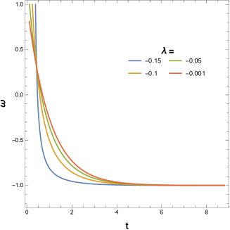
Figure 1: (Color online) Variation of $\omega_{1}$ with $t$ for $\tau=1$ and different values of $\lambda$ ($=-0.001,-0.05,-0.10,-0.15$)

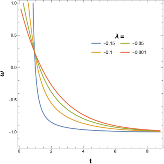
Figure 2: (Color online) Variation of $\omega_{1}$ with $t$ for $\tau=2$ and different values of $\lambda$ ($=-0.001,-0.05,-0.10,-0.15$)

In Figs. 1 and 2 we see that the value of $\omega$ starts with a positive one and ends up being constant at around $-1$. This curve shows the transition of $\omega$ from the radiation dominated era ($\omega=1/3$) to dark energy-dominated era ($\omega=-1$) through the matter-dominated era ($\omega=0$). These figures show that the value of $\omega$ decreases with time and takes negative values for each value of $\lambda$, which is satisfying from the observational viewpoint. The observational data [130] depicts that the value of the EoS parameter should take a value between $-0.95$ to $-1.13$ at the current epoch. Fig. 1 represents the variation of the EoS parameter for $\tau=1$ whereas Fig. 2 represents the variation of the same with $\tau=2$. In both the figures, we note that $\omega$ becomes constant at around $-0.95$ which is the observed value too. It is also observed that for more negative values of $\lambda$ the steepness of the curve is greater and when the value of $\lambda$ approaches zero the curve becomes less steep.

IV.2 $f(\bar{R},\bar{T})=\bar{R}+\alpha\bar{R}^{2}+\lambda\bar{T}$

This special type of $f(\bar{R})$ is known as the Starobinsky type model of modified gravity [136]. Interestingly, Starobinsky modified the Einstein-Hilbert action by considering the second-order term of Ricci scalar with a constant $\alpha$ [137]. He showed that a cosmological model obtained from the above consideration of $f(R)$ satisfies the cosmological observational tests. This model also forecasts an overproduction of scalarons in the very early universe. Considering axially symmetric dissipative dust under geodesic conditions, Sharif et al. [60] investigated the source of the gravitational radiation in the Starobinsky model. Therefore, we take this model into our consideration to check the cosmological scenarios for our case.

For this type of $f(\bar{R})$ we have

$$F(\bar{R})=1+2\alpha\bar{R};\leavevmode\nobreak\ \leavevmode\nobreak\ \dot{F}=2\alpha\dot{\bar{R}};\leavevmode\nobreak\ \leavevmode\nobreak\ \ddot{F}=2\alpha\ddot{\bar{R}}.$$ (41)

For this case, the Friedmann equation can be written from the $(00)$ and $(ii)$ component of the field equations (35) and (36). We can solve those Friedmann equation to get the expression of $\tilde{\rho}$ and $\tilde{p}$ in Appendix A (Eqs. 49 and 50), which immediately gives us the EoS parameter as

$$\omega_{2}=\frac{\tilde{p}_{2}}{\tilde{\rho_{2}}}=\frac{\omega_{N_{2}}}{\omega_{D_{2}}},$$ (42)

where $\tilde{\rho_{2}}$ and $\tilde{p}_{2}$ are energy density and pressure for the second choice of $f(\bar{R},\bar{T})$. The expression of $\omega_{2}$ has been given in Appendix A (Eqs. LABEL:A7 and 52).

The plots of $\omega_{2}$ vs. $t$ has been shown here. We choose two sets of the parameters:
I. $\tau=1$, $\lambda=1$, and $\alpha$ varies from $1,2,3,4,5$ (Fig. 3).
II. $\tau=1$, $\lambda=5$, $\alpha=1,2,3,4,5$ (Fig. 4).

From these figures, we see that both the curves become constant at $\omega_{2}=-1$ which is consistent with the observational data.

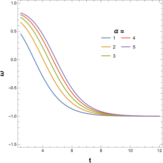
Figure 3: (Color online) Variation of $\omega_{2}$ with $t$ for $\tau=1$, $\lambda=1$ and different values of $\alpha=1,2,3,4,5$)

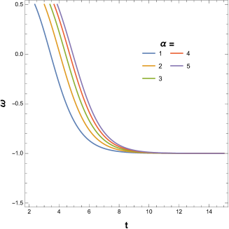
Figure 4: (Color online) Variation of $\omega_{2}$ with $t$ for $\tau=1$, $\lambda=5$ and different values of $\alpha$ ($=1,2,3,4,5$)

For this case, we varied the model parameter $\alpha$ keeping $\lambda$ fixed. If we look at the time scale we see that for a greater value of $\alpha$ the transition from radiation ($\omega=1/3$) to dark energy-dominated era ($\omega=-1$) is delayed. So the greater contribution of the higher order term of Ricci scalar ($\bar{R}$) makes the EoS parameter decrease at the late time of evolution.

IV.3 Generalising the choice of $f(\bar{R},\bar{T})$

Now we want to generalize the form of the function $f(\bar{R},\bar{T})$ and check the validity of each model depending on the integer values of $n$. We take $f(\bar{R},\bar{T})$ as

$$f(\bar{R},\bar{T})=\bar{R}+\alpha\bar{R}^{n}+\lambda\bar{T}.$$ (43)

For Eq. (43) we get, $F=\frac{\partial f(\bar{R},\bar{T})}{\partial\bar{R}}=1+n\alpha\bar{R}^{n-1},\\ \leavevmode\nobreak\ \dot{F}=\frac{\partial F}{\partial t}=\alpha n(n-1)\bar{R}^{n-2}\dot{\bar{R}},\\ \leavevmode\nobreak\ \ddot{F}=\frac{\partial^{2}F}{\partial t^{2}}=\alpha n(n-1)\Big{(}(n-2)\bar{R}^{n-3}+\bar{R}^{n-2}\ddot{\bar{R}}\Big{)}$

Considering Eqs. (37), (38) and (39), for the above choice of $f(\bar{R},\bar{T})$ (43), we have the EoS parameter

$$\omega_{3}=\frac{\omega_{N_{3}}}{\omega_{D_{3}}},$$ (44)

where the explicit forms of $\omega_{N_{3}}$ and $\omega_{D_{3}}$ are expressed in (53) and (54) respectively.

We want to check the validity of our model with observational data set [130] for general choice of $f(\bar{R},\bar{T})$ (43) depending on model parameters, which give us some valid plots between $\omega$ and time. We have four parameters here which are $\tau,\leavevmode\nobreak\ \alpha,\leavevmode\nobreak\ \lambda,\leavevmode\nobreak\ \&\leavevmode\nobreak\ n$. The constraints in choosing these parameters are mentioned below:

Parameter	Constraint	Possible Values
$\tau$	can only be positive integer	$1\leavevmode\nobreak\ \&\leavevmode\nobreak\ 10$
$\alpha$	can be positive mostly	$1\leavevmode\nobreak\ \&\leavevmode\nobreak\ 10$
$\lambda$	can be any rational number	$-10,\leavevmode\nobreak\ -0.1,\leavevmode\nobreak\ 0.1,\leavevmode\nobreak\ \&\leavevmode\nobreak\ 10$
$n$	can be positive integers mostly	$0-10$

Table 1: Table for possible values of model parameters

These choices of model parameters provide us opportunity to combine them in various ways to get different graphs of $\omega$. With these parameters, we get $32$ set of parameters which have been mentioned in Table II. From those $32$ sets, we get physical and viable graph for $16$ set of parameters only. We have mentioned which set of parameters give us a valid plot of $\omega$ vs. $t$ which actually satisfies the observational data. From Table II, we see that a large value of $\tau$ is not a preferable choice because for large value of $\tau$ graphs do not satisfy with the observational data. Now we plot these 16 graphs below:

$\tau$	$\alpha$	$\lambda$	$n$	validity
$1$	$1$	$-10$	$0,2,4,6,8,10$	valid (Plot 9)
			$1,3,5,7,9$	valid (Plot 1)
$10$	$1$	$-10$	$0,2,4,6,8,10$	invalid
			$1,3,5,7,9$	invalid
$1$	$10$	$-10$	$0,2,4,6,8,10$	valid (Plot 10)
			$1,3,5,7,9$	valid (Plot 2)
$10$	$10$	$-10$	$0,2,4,6,8,10$	invalid
			$1,3,5,7,9$	invalid
$1$	$1$	$-0.1$	$0,2,4,6,8,10$	valid (Plot 11)
			$1,3,5,7,9$	valid (Plot.3)
$10$	$1$	$-0.1$	$0,2,4,6,8,10$	invalid
			$1,3,5,7,9$	invalid
$1$	$10$	$-0.1$	$0,2,4,6,8,10$	valid (Plot 12)
			$1,3,5,7,9$	valid (Plot.4)
$10$	$10$	$-0.1$	$0,2,4,6,8,10$	invalid
			$1,3,5,7,9$	invalid
$1$	$1$	$0.1$	$0,2,4,6,8,10$	valid (Plot 13)
			$1,3,5,7,9$	valid (Plot 5)
$10$	$1$	$0.1$	$0,2,4,6,8,10$	invalid
			$1,3,5,7,9$	invalid
$1$	$10$	$0.1$	$0,2,4,6,8,10$	valid (Plot 14)
			$1,3,5,7,9$	valid (Plot 6)
$10$	$10$	$0.1$	$0,2,4,6,8,10$	invalid
			$1,3,5,7,9$	invalid
$1$	$1$	$10$	$0,2,4,6,8,10$	valid (Plot 15)
			$1,3,5,7,9$	valid (Plot.7)
$10$	$1$	$10$	$0,2,4,6,8,10$	invalid
			$1,3,5,7,9$	invalid
$1$	$10$	$10$	$0,2,4,6,8,10$	valid (Plot 16)
			$1,3,5,7,9$	valid (Plot 8)
$10$	$10$	$10$	$0,2,4,6,8,10$	invalid
			$1,3,5,7,9$	invalid

Table 2: Table for a possible set of model parameters which are valid or invalid based on plots.

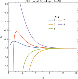
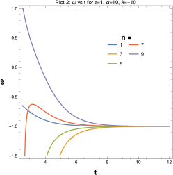
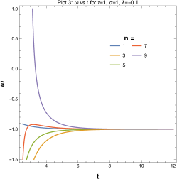
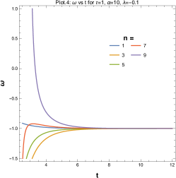
Figure 5: (Color online) Variation of $\omega$ with $t$ for different model parameters for odd $n$

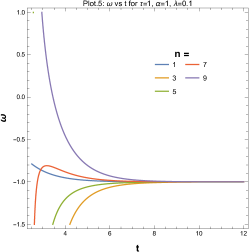
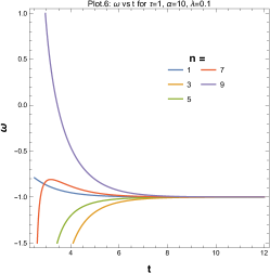
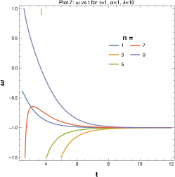
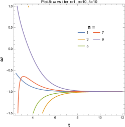
Figure 6: (Color online) Variation of $\omega$ with $t$ for different model parameters for odd $n$

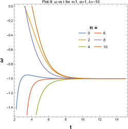
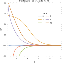
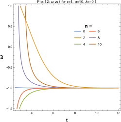
Figure 7: (Color online) Variation of $\omega$ with $t$ for different model parameters for even $n$

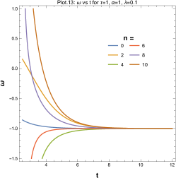
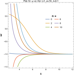
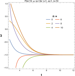
Figure 8: (Color online) Variation of $\omega$ with $t$ for different model parameters for even $n$

Analyzing every graph (Figs. 5, 6, 7 and 8) shown above we note that in each case the observational data for late time acceleration are satisfied by the lower ($n$=0, 1, 2) and higher ($n$=8, 9, 10) value of $n$. The mid-value of $n$(=3, 4, 5, 6 and 7) produces curves that start from the negative value of $\omega$. When the power of $\bar{R}$ varies in lower order the curvature is small and when the power of $\bar{R}$ is high the curvature varies extensively where $\bar{R}$ denotes the curvature in the action. Now for both the lower ($n$=0, 1, 2) and higher ($n$=8, 9, 10) curvatures, we get the observation-satisfied result at the present epoch. Generally, high curvature indicates that the effect of gravity is strong which may be a region around dense objects. For $n=7$ shows a peculiar variation of EoS parameter for some plots, i.e., it starts from a large negative value, then crossed the $-1$ value, and goes upward, then again it becomes constant at $-1$. The mid-value of $n$, i.e., $n$=3, 4, 5, 6 and 7 shows the EoS parameter starts from high negative to $-1$, which is the present value of EoS parameter of the universe. This indicates that the early universe may be dark energy dominated. This may justify the kinetically driven inflation, i.e. K-inflation scenario [110], which means the kinetically driven inflation rolls gracefully from a high-curvature starting phase to a low-curvature phase and may eventually leave inflation to become radiation-dominated. So we may conclude that our model is valid for the entire range of the universe which means starting from the early (ultra relativistic era) to the present epoch (dark energy dominated era). It should be noted that in the above pictures, the time denotes cosmic time and has not been scaled, and $t\to 0$ on this axis indicates the early universe.

IV.4 Observational Verification of the models at present epoch

In this sub-section, we compare our results for different choices of $f(\bar{R},\bar{T})$ with the observational data sets [130].

$\tau$	$\lambda$	$t$	$\omega_{1}$ ($3\sigma$ confidence)[130]	Observation [130]
$1$	$-0.15$	1.91077	$-0.95\geq\omega\geq-1.13$	SNIa+ BAO+ H(z)
	$-0.1$	3.02237
	$-0.01$	3.64823
	$-0.001$	3.68496
$2$	$-0.15$	3.57211	$-0.95\geq\omega\geq-1.13$	SNIa+ BAO+ H(z)
	$-0.10$	5.98057
	$-0.01$	7.29301
	$-0.001$	7.36959

Table 3: Table for observational verification of the model for $f(\bar{R},\bar{T})=\bar{R}+\lambda\bar{T}$ for $\tau=1,2$ and $\lambda=-0.10,-0.11,-0.12,-0.13,-0.14,-0.15$.

$\tau$	$\lambda$	$\alpha$	$t$	$\omega_{1}$ ($3\sigma$ confidence)[130]	Observation [130]
$1$	$1$	$1$	6.9989215500337565	$-0.95\geq\omega\geq-1.13$	SNIa+ BAO+ H(z)
		$2$	7.648323690317918
		$3$	8.038769314737097
		$4$	8.318855798895852
		$5$	8.53741401857794
$1$	$5$	$1$	$6.9989215500337565$	$-0.95\geq\omega\geq-1.13$	SNIa+ BAO+ H(z)
		$2$	7.648323690317918
		$3$	8.038769314737097
		$4$	8.318855798895852
		$5$	8.53741401857794

Table 4: Table for observational verification of the model for $f(\bar{R},\bar{T})=\bar{R}+\alpha\bar{R}^{2}+\lambda\bar{T}$ for $\tau=1$, $\lambda=1,5$ and $\alpha=1,2,3,4,5$.

Tables III and IV indicate how well our model matches to the observational data as available in Ref. [130]. We used the EoS parameter data from the combined observations of SNIa, BAO, and H(z), which indicates that for the current accelerating universe, the EoS parameter should have a value in the range $-0.95\geq\omega\geq-1.13$. We found that for certain parameter selections, we may attain a time range in which the above-mentioned value of $\omega$ is satisfied. So, for the above two situations, we can state unequivocally that our model is very much compatible with the observable evidence at the current epoch.

V Conclusion and Discussion

In a nutshell, in this paper, we have tried to formulate the $f(\bar{R},\bar{T})$ gravity theory in a non-standard theory (i.e. K-essence theory). Starting with a brief review of the K-essence theory for a special type of non-canonical Lagrangian (i.e. DBI type), we entered into our work, which is to establish a different form of the well-known $f(\bar{R},\bar{T})$ gravity theory by the metric formalism. Taking the action of the modified gravity in the context of K-essence geometry and following [40], we have presented the modified field equations of our case (24). One can easily find that the field equations of our case is different from the standard field equations of $f(R,T)$ gravity [39, 40] due to the presence of the K-essence scalar field.

Not only that, it is also crystal clear that the field equations of usual $f(R,T)$ gravity can be recovered from (24), if we consider the K-essence scalar field ($\phi$) terms to be zero and the Lagrangian as $L_{m}=p$. Here we would like to mention that, according to Refs.[81, 82, 83, 37, 133], the kinetic energy of the K-essence scalar field ($\dot{\phi}^{2}$), considered as the dark energy density (in the unit of critical density) of the present universe. Similar to the works [39] and [40], the covariant derivative of the energy-momentum tensor has also been calculated for our case which, for obvious reasons, turns out to be of different from [39] and [40]. We get some extra terms related to the scalar field ($\phi$), which may reveal some more astonishing features of this theory. These extra terms are appeared due to interactions of the usual gravity with the K-essence scalar field.

We have solved the field equations by considering the background metric as the flat FLRW type and computed the Friedmann equations of our theory for the general form of $f(\bar{R},\bar{T})$. We also have established a new definition of $\bar{\Theta}_{\mu\nu}$ in (34), which is not so straightforward as obtained in [39] and [40]. As the Lagrangian for our case has an implicit dependence on the scalar field $\phi$ of the K-essence geometry, specifically it has explicit dependence on the derivative of $\phi$, some extra features are included in it automatically. In this process, we have used some important relations, which connect the usual geometry with the K-essence geometry already showed in [81, 82].

The next part of our work includes the evaluation of the EoS parameter by solving the Friedmann equations obtained in (37) and (38), where we have considered general form of $f(\bar{R},\bar{T})$. We get far different results from what has been achieved by Sahoo et al. [39] in their Eqs. (13) and (14). Following [132], we have expressed $\dot{\phi}^{2}$ as an exponential function of time (39) which satisfy the conditions for $\dot{\phi}^{2}\leavevmode\nobreak\ (0<\dot{\phi}^{2}<1)$. Next, we have found the variation of the EoS parameter by choosing different forms of $f(\bar{R},\bar{T})$. Particularly, we have taken three choices of $f(\bar{R},\bar{T})$, of which the first one is the simple case, i.e., $f(\bar{R},\bar{T})=\bar{R}+\lambda\bar{T}$ (Section: IV, Case A), the second one is of Starobinsky type $f(\bar{R})$, i.e., $f(\bar{R},\bar{T})=\bar{R}+\alpha\bar{R}^{2}+\lambda\bar{T}$ (Section: IV, Case B) and third one is more general form, i.e., $f(\bar{R},\bar{T})=\bar{R}+\alpha\bar{R}^{n}+\lambda\bar{T}$ (Section: IV, Case C).

It is a well-known fact, that for our the present universe, which has a positive acceleration, the value of the EoS parameter is $\omega\leq-1$. So to check the efficacy of our results we have plotted the variation of this EoS parameter obtained in this paper in Section IV. For each consideration of $f(\bar{R},\bar{T})$, we first set the required parameter values and then we draw the graph of $\omega$ vs. $t$. In Case C, we analyse a generic form of $f(\bar{R},\bar{T})$ and demonstrate through the plots that our model is consistent with the empirical data for particular model parameter choices. Then in Section IVD we matched the obtained graphs for first two choices of $f(\bar{R},\bar{T})$ in Table III and Table IV with the observational data taken from [130]. Note that in these graphs we have taken $t\rightarrow 0$ as the early time of the universe. It is also have mentioned that upto Eq. (25), we have constructed a generalized non-canonical $f(\bar{R},\bar{T})$ theory on the basis of specific DBI type non-standard action in an emergent K-essence geometry. The next portion is a special case study of this theory under the consideration of the relation between the Hubble parameter and the K-essence scalar field where we have assumed the background gravitational metric to be flat FLRW type.

From a totally different background, we establish the $f(\bar{R},\bar{T})$ theory of modified gravity with dark energy consideration in a new packet. The achievement of this work lies in the fact that without considering the cosmological constant model we are able to produce a theory that supports the results of present observational data. It is also noted that the K-essence theory is observationally tested through the Planck collaboration results: 2015-XIV [4], 2018-VI [5]. From the results and graphs obtained here, we see that there are some choices of model parameters ($\lambda,\tau,\alpha$) for which we get $\omega\leq-1$, which satisfy the observational data to a large extent.

The mid-value of $n$, or $n$=3, 4, 5, 6, 7, indicates that the EoS parameter begins from high negative to $-1$, which is the current value of the EoS parameter of the universe, for the general case of $f(\bar{R},\bar{T})$ (Case C). This suggests that dark energy could have been dominant in the early cosmos. This may support the kinetically driven inflation, often known as the K-inflation scenario [110], which smoothly transitions from a high-curvature initial phase to a low-curvature intermediate phase before leaving inflation to become radiation-dominated. We may thus draw the conclusion that our model holds true for the evolution of the entire phases of the universe, beginning from the early era and ending in the present. It has also been noted that this theory may be used not just in the context of dark energy, but also from a purely gravitational standpoint [132, 134, 135], since the existence of dark energy in the context of cosmology is still a matter of debate [138].

In the article we have not addressed the behavior of the additional cosmological parameters, like the Hubble parameter, the deceleration parameter, redshift function and so on, which however can be taken into account in the near future. For the time being, based on all the features and attributes of the present investigation, we may conclude that our model provides possibilities for a new viewpoint of the cosmological and gravitational scenario.

appendix

Expressions of full forms of the EoS parameters for various models of $f(\bar{R})$

V.1 $f(\bar{R})=\bar{R}$

The expression of $\tilde{\rho}_{1}$ and $\tilde{p}_{1}$ is given by:

$$\tilde{p}_{1} =\frac{1}{\Big{(}48\lambda^{2}+16\lambda+1\Big{)}\dot{\phi}^{2}\Big{(}\dot{\phi}^{2}-1\Big{)}^{3}}\Big{[}2\Big{(}8\lambda^{2}\sqrt{1-\dot{\phi}^{2}}\dot{\phi}^{12}-24\lambda^{2}\sqrt{1-\dot{\phi}^{2}}\dot{\phi}^{10}+2\lambda\dot{\phi}^{8}\Big{(}\lambda\Big{(}7\sqrt{1-\dot{\phi}^{2}}-4\Big{)}+\sqrt{1-\dot{\phi}^{2}}-1\Big{)}$$ (45)

$$+2\lambda\dot{\phi}^{6}\Big{(}\lambda\Big{(}12-7\sqrt{1-\dot{\phi}^{2}}\Big{)}-3\sqrt{1-\dot{\phi}^{2}}+3\Big{)}+6\lambda(4\lambda+1)\Big{(}\sqrt{1-\dot{\phi}^{2}}-1\Big{)}\dot{\phi}^{4}-2(6\lambda+1)\dot{\ddot{\phi}}\dot{\phi}^{3}+2(6\lambda+1)\dot{\ddot{\phi}}\dot{\phi}$$

$$+\dot{\phi}^{2}\Big{(}8(6\lambda+1)\ddot{\phi}^{2}-2\lambda(4\lambda+1)\Big{(}\sqrt{1-\dot{\phi}^{2}}-1\Big{)}\Big{)}+\ddot{\phi}^{2}\Big{)}\Big{]}$$

$$\tilde{\rho_{1}} =\frac{1}{\Big{(}48\lambda^{2}+16\lambda+1\Big{)}\dot{\phi}^{2}\Big{(}\dot{\phi}^{2}-1\Big{)}^{3}}\Big{[}2\Big{(}-3(8\lambda+1)\ddot{\phi}^{2}+4\lambda(10\lambda+1)\sqrt{1-\dot{\phi}^{2}}\dot{\phi}^{12}-12\lambda(10\lambda+1)\sqrt{1-\dot{\phi}^{2}}\dot{\phi}^{10}$$ (46)

$$+\lambda\dot{\phi}^{8}\Big{(}\lambda\Big{(}22\sqrt{1-\dot{\phi}^{2}}+8\Big{)}+\sqrt{1-\dot{\phi}^{2}}+2\Big{)}+\lambda\dot{\phi}^{6}\Big{(}\lambda\Big{(}74\sqrt{1-\dot{\phi}^{2}}-24\Big{)}+11\sqrt{1-\dot{\phi}^{2}}-6\Big{)}$$

$$-6\lambda(4\lambda+1)\Big{(}\sqrt{1-\dot{\phi}^{2}}-1\Big{)}\dot{\phi}^{4}-12\lambda\dot{\ddot{\phi}}\dot{\phi}^{3}+12\lambda\dot{\ddot{\phi}}\dot{\phi}+2\lambda\dot{\phi}^{2}\Big{(}(4\lambda+1)\Big{(}\sqrt{1-\dot{\phi}^{2}}-1\Big{)}+24\ddot{\phi}^{2}\Big{)}\Big{)}\Big{]}.$$

Using Eqs. (45), (46) and (39), we have the numerator and denominator of Eq. (40) as:

$$\omega_{N_{1}} = -96\lambda^{2}\tau^{2}e^{t/\tau}\sqrt{1-e^{-\frac{t}{\tau}}}+32\lambda^{2}\tau^{2}\sqrt{1-e^{-\frac{t}{\tau}}}-8\lambda\tau^{2}e^{\frac{3t}{\tau}}\Big{(}-12\lambda+7\lambda\sqrt{1-e^{-\frac{t}{\tau}}}+3\sqrt{1-e^{-\frac{t}{\tau}}}-3\Big{)}$$ (47)

$$+8\lambda\tau^{2}e^{\frac{2t}{\tau}}\Big{(}\lambda\Big{(}7\sqrt{1-e^{-\frac{t}{\tau}}}-4\Big{)}+\sqrt{1-e^{-\frac{t}{\tau}}}-1\Big{)}-(4\lambda+1)e^{\frac{5t}{\tau}}\Big{(}8\lambda\tau^{2}\Big{(}\sqrt{1-e^{-\frac{t}{\tau}}}-1\Big{)}-3\Big{)}$$

$$+6e^{\frac{4t}{\tau}}\Big{(}6\lambda+4\lambda(4\lambda+1)\tau^{2}\Big{(}\sqrt{1-e^{-\frac{t}{\tau}}}-1\Big{)}+1\Big{)}.$$

$$\omega_{D_{1}} = -48\lambda(10\lambda+1)\tau^{2}e^{t/\tau}\sqrt{1-e^{-\frac{t}{\tau}}}+4\lambda\tau^{2}e^{\frac{2t}{\tau}}\Big{(}\lambda\Big{(}22\sqrt{1-e^{-\frac{t}{\tau}}}+8\Big{)}+\sqrt{1-e^{-\frac{t}{\tau}}}+2\Big{)}+4\lambda\tau^{2}e^{\frac{3t}{\tau}}\Big{(}\lambda\Big{(}74\sqrt{1-e^{-\frac{t}{\tau}}}-24\Big{)}$$ (48)

$$+11\sqrt{1-e^{-\frac{t}{\tau}}}-6\Big{)}+16\lambda(10\lambda+1)\tau^{2}\sqrt{1-e^{-\frac{t}{\tau}}}+(4\lambda+1)e^{\frac{5t}{\tau}}\Big{(}8\lambda\tau^{2}\Big{(}\sqrt{1-e^{-\frac{t}{\tau}}}-1\Big{)}-3\Big{)}$$

$$-12\lambda e^{\frac{4t}{\tau}}\Big{(}2(4\lambda+1)\tau^{2}\Big{(}\sqrt{1-e^{-\frac{t}{\tau}}}-1\Big{)}-3\Big{)}.$$

V.2 $f(\bar{R})=\bar{R}+\alpha\bar{R}^{2}$

The expression of $\tilde{\rho}_{2}$ and $\tilde{p}_{2}$ is given by:

$$\tilde{p}_{2} = \frac{2}{\Big{(}48\lambda^{2}+16\lambda+1\Big{)}\dot{\phi}^{4}\Big{(}\dot{\phi}^{2}-1\Big{)}^{6}}\Big{[}18\alpha(12\lambda+1)\ddot{\phi}^{4}+4(6\lambda+1)\Big{(}2\dot{\ddot{\phi}}-3\alpha\dot{\ddot{\ddot{\phi}}}\Big{)}\dot{\phi}^{9}-72\alpha(7\lambda+1)\dot{\ddot{\phi}}\dot{\phi}\ddot{\phi}^{2}$$ (49)

$$-12(6\lambda+1)\dot{\phi}^{7}\Big{(}\dot{\ddot{\phi}}\Big{(}124\alpha\ddot{\phi}^{2}+1\Big{)}-3\alpha\dot{\ddot{\ddot{\phi}}}\Big{)}+4\dot{\phi}^{5}\Big{(}2\dot{\ddot{\phi}}\Big{(}6\lambda+3\alpha(219\lambda+32)\ddot{\phi}^{2}+1\Big{)}-9\alpha(6\lambda+1)\dot{\ddot{\ddot{\phi}}}\Big{)}$$

$$+2\dot{\phi}^{3}\Big{(}6\alpha(6\lambda+1)\dot{\ddot{\ddot{\phi}}}+\dot{\ddot{\phi}}\Big{(}-6\lambda+36\alpha(58\lambda+11)\ddot{\phi}^{2}-1\Big{)}\Big{)}+\dot{\phi}^{8}\Big{(}156(6\alpha\lambda+\alpha)\dot{\ddot{\phi}}^{2}+192\alpha(6\lambda+1)\ddot{\ddot{\phi}}\ddot{\phi}-(144\lambda+23)\ddot{\phi}^{2}$$

$$+10\lambda\Big{(}-12\lambda+11\lambda\sqrt{1-\dot{\phi}^{2}}+3\sqrt{1-\dot{\phi}^{2}}-3\Big{)}\Big{)}-3\dot{\phi}^{6}\Big{(}2\alpha(288\lambda+49)\dot{\ddot{\phi}}(t)^{2}-480(6\alpha\lambda+\alpha)\ddot{\phi}^{4}+24\alpha(31\lambda+5)\ddot{\ddot{\phi}}\ddot{\phi}$$

$$-(48\lambda+7)\ddot{\phi}^{2}+4\lambda(4\lambda+1)\Big{(}\sqrt{1-\dot{\phi}^{2}}-1\Big{)}\Big{)}+\dot{\phi}^{4}\Big{(}24\alpha(27\lambda+5)\dot{\ddot{\phi}}^{2}+96\alpha(90\lambda+17)\ddot{\phi}^{4}+144\alpha(7\lambda+1)\ddot{\ddot{\phi}}\ddot{\phi}-(48\lambda+5)\ddot{\phi}^{2}$$

$$+2\lambda(4\lambda+1)\Big{(}\sqrt{1-\dot{\phi}^{2}}-1\Big{)}\Big{)}+\dot{\phi}^{2}\Big{(}18\alpha(8\lambda+1)\dot{\ddot{\phi}}^{2}-24\alpha(54\lambda+5)\ddot{\phi}^{4}+24\alpha(3\lambda+1)\ddot{\ddot{\phi}}\ddot{\phi}-\ddot{\phi}^{2}\Big{)}+8\lambda^{2}\sqrt{1-\dot{\phi}^{2}}\dot{\phi}^{20}$$

$$-48\lambda^{2}\sqrt{1-\dot{\phi}^{2}}\dot{\phi}^{18}+2\lambda\dot{\phi}^{16}\Big{(}\lambda\Big{(}55\sqrt{1-\dot{\phi}^{2}}-4\Big{)}+\sqrt{1-\dot{\phi}^{2}}-1\Big{)}-4\lambda\dot{\phi}^{14}\Big{(}-12\lambda+34\lambda\sqrt{1-\dot{\phi}^{2}}+3\sqrt{1-\dot{\phi}^{2}}-3\Big{)}$$

$$+6\lambda\dot{\phi}^{12}\Big{(}-20\lambda+22\lambda\sqrt{1-\dot{\phi}^{2}}+5\sqrt{1-\dot{\phi}^{2}}-5\Big{)}-2(6\lambda+1)\dot{\ddot{\phi}}\dot{\phi}^{11}-8\dot{\phi}^{10}\Big{(}\lambda\Big{(}-20\lambda+17\lambda\sqrt{1-\dot{\phi}^{2}}+5\sqrt{1-\dot{\phi}^{2}}-5\Big{)}$$

$$-(6\lambda+1)\ddot{\phi}^{2}\Big{)}\Big{]},$$

$$\tilde{\rho}_{2} = \frac{2}{\Big{(}48\lambda^{2}+16\lambda+1\Big{)}\dot{\phi}^{4}\Big{(}\dot{\phi}^{2}-1\Big{)}^{6}}\Big{[}54\alpha(12\lambda+1)\ddot{\phi}^{4}+24\lambda\Big{(}2\dot{\ddot{\phi}}-3\alpha\dot{\ddot{\ddot{\phi}}}\Big{)}\dot{\phi}^{9}-36\alpha(22\lambda+1)\dot{\ddot{\phi}}\dot{\phi}\ddot{\phi}^{2}-72\lambda\dot{\phi}^{7}\Big{(}\dot{\ddot{\phi}}\Big{(}124\alpha\ddot{\phi}^{2}+1\Big{)}$$ (50)

$$-3\alpha\dot{\ddot{\ddot{\phi}}}\Big{)}+12\dot{\phi}^{5}\Big{(}\dot{\ddot{\phi}}\Big{(}4\lambda+3\alpha(218\lambda+9)\ddot{\phi}^{2}\Big{)}-18\alpha\lambda\dot{\ddot{\ddot{\phi}}}\Big{)}+12\dot{\phi}^{3}\Big{(}6\alpha\lambda\phi^{(5)}(t)+\dot{\ddot{\phi}}\Big{(}12\alpha(13\lambda-2)\ddot{\phi}^{2}-\lambda\Big{)}\Big{)}$$

$$+\dot{\phi}^{8}\Big{(}936\alpha\lambda\dot{\ddot{\phi}}^{2}+1152\alpha\lambda\ddot{\ddot{\phi}}\ddot{\phi}-3(56\lambda+1)\ddot{\phi}^{2}-5\lambda\Big{(}\lambda\Big{(}34\sqrt{1-\dot{\phi}^{2}}-24\Big{)}+7\sqrt{1-\dot{\phi}^{2}}-6\Big{)}\Big{)}+3\dot{\phi}^{6}\Big{(}6\alpha(1-88\lambda)\dot{\ddot{\phi}}^{2}$$

$$+2880\alpha\lambda\ddot{\phi}^{4}-12\alpha(70\lambda+1)\ddot{\ddot{\phi}}\ddot{\phi}+(72\lambda+3)\ddot{\phi}^{2}+4\lambda(4\lambda+1)\Big{(}\sqrt{1-\dot{\phi}^{2}}-1\Big{)}\Big{)}+\dot{\phi}^{4}\Big{(}36\alpha(10\lambda-1)\dot{\ddot{\phi}}^{2}+576\alpha(7\lambda-1)\ddot{\phi}^{4}$$

$$+72\alpha(22\lambda+1)\ddot{\ddot{\phi}}\ddot{\phi}-3(40\lambda+3)\ddot{\phi}^{2}-2\lambda(4\lambda+1)\Big{(}\sqrt{1-\dot{\phi}^{2}}-1\Big{)}\Big{)}-3\dot{\phi}^{2}\Big{(}-6\alpha(16\lambda+1)\dot{\ddot{\phi}}^{2}+48\alpha(25\lambda+2)\ddot{\phi}^{4}$$

$$+12\alpha(6\lambda+1)\ddot{\ddot{\phi}}\ddot{\phi}-(8\lambda+1)\ddot{\phi}^{2}\Big{)}+4\lambda(10\lambda+1)\sqrt{1-\dot{\phi}^{2}}\dot{\phi}^{20}-24\lambda(10\lambda+1)\sqrt{1-\dot{\phi}^{2}}\dot{\phi}^{18}+\lambda\dot{\phi}^{16}\Big{(}\lambda\Big{(}502\sqrt{1-\dot{\phi}^{2}}+8\Big{)}$$

$$+49\sqrt{1-\dot{\phi}^{2}}+2\Big{)}-4\lambda\dot{\phi}^{14}\Big{(}2\lambda\Big{(}49\sqrt{1-\dot{\phi}^{2}}+6\Big{)}+8\sqrt{1-\dot{\phi}^{2}}+3\Big{)}-6\lambda\dot{\phi}^{12}\Big{(}10\lambda\Big{(}\sqrt{1-\dot{\phi}^{2}}-2\Big{)}+4\sqrt{1-\dot{\phi}^{2}}-5\Big{)}$$

$$-12\lambda\dot{\ddot{\phi}}\dot{\phi}^{11}+4\lambda\dot{\phi}^{10}\Big{(}10\lambda\Big{(}7\sqrt{1-\dot{\phi}^{2}}-4\Big{)}+12\ddot{\phi}^{2}+13\sqrt{1-\dot{\phi}^{2}}-10\Big{)}\Big{)}\Big{]}.$$

Using Eqs. (49), (50) and (39), different parts of Eq. (42) has been expressed as:

$$\omega_{N_{2}} = 6e^{\frac{7t}{\tau}}\Big{(}-15\alpha(24\lambda+5)-\tau^{2}+16\lambda(4\lambda+1)\tau^{4}\Big{(}\sqrt{1-e^{-\frac{t}{\tau}}}-1\Big{)}\Big{)}-e^{\frac{6t}{\tau}}\Big{(}27\alpha(188\lambda+33)+18(8\lambda+1)\tau^{2}$$

$$+80\lambda\tau^{4}\Big{(}-12\lambda+11\lambda\sqrt{1-e^{-\frac{t}{\tau}}}+3\sqrt{1-e^{-\frac{t}{\tau}}}-3\Big{)}\Big{)}+2e^{\frac{5t}{\tau}}\Big{(}-72\alpha(6\lambda+1)+3(32\lambda+5)\tau^{2}+32\lambda\tau^{4}\Big{(}-20\lambda$$

$$+17\lambda\sqrt{1-e^{-\frac{t}{\tau}}}+5\sqrt{1-e^{-\frac{t}{\tau}}}-5\Big{)}\Big{)}+384\lambda^{2}\tau^{4}e^{t/\tau}\sqrt{1-e^{-\frac{t}{\tau}}}-64\lambda^{2}\tau^{4}\sqrt{1-e^{-\frac{t}{\tau}}}+32\lambda\tau^{4}e^{\frac{3t}{\tau}}\Big{(}-12\lambda$$

$$+34\lambda\sqrt{1-e^{-\frac{t}{\tau}}}+3\sqrt{1-e^{-\frac{t}{\tau}}}-3\Big{)}-16\lambda\tau^{4}e^{\frac{2t}{\tau}}\Big{(}\lambda\Big{(}55\sqrt{1-e^{-\frac{t}{\tau}}}-4\Big{)}+\sqrt{1-e^{-\frac{t}{\tau}}}-1\Big{)}$$

$$-2(4\lambda+1)\tau^{2}e^{\frac{8t}{\tau}}\Big{(}8\lambda\tau^{2}\Big{(}\sqrt{1-e^{-\frac{t}{\tau}}}-1\Big{)}-3\Big{)}-12\tau^{2}e^{\frac{4t}{\tau}}\Big{(}6\lambda+4\lambda\tau^{2}\Big{(}-20\lambda+22\lambda\sqrt{1-e^{-\frac{t}{\tau}}}+5\sqrt{1-e^{-\frac{t}{\tau}}}-5\Big{)}+1\Big{)},$$

$$\omega_{D_{2}} = -6e^{\frac{7t}{\tau}}\Big{(}-45\alpha-3(8\lambda+1)\tau^{2}+16\lambda(4\lambda+1)\tau^{4}\Big{(}\sqrt{1-e^{-\frac{t}{\tau}}}-1\Big{)}\Big{)}+e^{\frac{6t}{\tau}}\Big{(}27\alpha(5-148\lambda)-18(16\lambda+1)\tau^{2}$$ (52)

$$+40\lambda\tau^{4}\Big{(}-24\lambda+34\lambda\sqrt{1-e^{-\frac{t}{\tau}}}+7\sqrt{1-e^{-\frac{t}{\tau}}}-6\Big{)}\Big{)}+e^{\frac{5t}{\tau}}\Big{(}6\tau^{2}+16\lambda\Big{(}-54\alpha+15\tau^{2}+\tau^{4}\Big{(}20\lambda\Big{(}4-7\sqrt{1-e^{-\frac{t}{\tau}}}\Big{)}$$

$$-26\sqrt{1-e^{-\frac{t}{\tau}}}+20\Big{)}\Big{)}\Big{)}+32\lambda\tau^{4}e^{\frac{3t}{\tau}}\Big{(}2\lambda\Big{(}49\sqrt{1-e^{-\frac{t}{\tau}}}+6\Big{)}+8\sqrt{1-e^{-\frac{t}{\tau}}}+3\Big{)}-8\lambda\tau^{4}e^{\frac{2t}{\tau}}\Big{(}\lambda\Big{(}502\sqrt{1-e^{-\frac{t}{\tau}}}+8\Big{)}$$

$$+49\sqrt{1-e^{-\frac{t}{\tau}}}+2\Big{)}+192\lambda(10\lambda+1)\tau^{4}e^{t/\tau}\sqrt{1-e^{-\frac{t}{\tau}}}-32\lambda(10\lambda+1)\tau^{4}\sqrt{1-e^{-\frac{t}{\tau}}}+2(4\lambda+1)\tau^{2}e^{\frac{8t}{\tau}}\Big{(}8\lambda\tau^{2}$$

$$\Big{(}\sqrt{1-e^{-\frac{t}{\tau}}}-1\Big{)}-3\Big{)}+24\lambda\tau^{2}e^{\frac{4t}{\tau}}\Big{(}2\tau^{2}\Big{(}10\lambda\Big{(}\sqrt{1-e^{-\frac{t}{\tau}}}-2\Big{)}+4\sqrt{1-e^{-\frac{t}{\tau}}}-5\Big{)}-3\Big{)}.$$

V.3 $f(\bar{R},\bar{T})=\bar{R}+\alpha\bar{R}^{n}+\lambda\bar{T}$

As per the similar calculations of the above types of $f(\bar{R},\bar{T})$ we have the EoS parameter ($\omega$) for this choice of $f(\bar{R},\bar{T})$ can be expressed as follows $\omega=\frac{\omega_{N_{3}}}{\omega_{D_{3}}}$ where

$$\omega_{N_{3}} =12(e^{-t}-1)\Bigg{[}2^{-n-1}3^{n}\Big{[}\frac{e^{2t}(2e^{t}-3)}{(e^{t}-1)^{3}}\Big{]}^{n}$$ (53)

$$+\frac{1}{(2e^{t}-3)^{3}}\Big{[}2^{3-n}3^{n-1}(n-1)ne^{-3t}\Big{\{}(n-4)e^{5t}+9(n-2)e^{t}+14(n-1)e^{3t}+(15-6n)e^{4t}$$

$$+(11-16n)e^{2t}-2n+4\Big{\}}\Big{(}\frac{e^{2t}(2e^{t}-3)}{(e^{t}-1)^{3}}\Big{)}^{n}\Big{]}-\frac{1}{(3-2e^{t})^{2}}\Big{\{}\Big{(}\frac{3}{2}\Big{)}^{n}(n-1)n(e^{t}-2)\Big{(}\frac{e^{2t}(2e^{t}-3)}{(e^{t}-1)^{3}}\Big{)}^{n}\Big{\}}$$

$$+\frac{1}{2(1-e^{-t})^{3}}\Big{[}3(e^{-t}-1)\Big{\{}n\Big{(}\frac{2}{3}\Big{)}^{1-n}\Big{(}\frac{e^{2t}(2e^{t}-3)}{(e^{t}-1)^{3}}\Big{)}^{n-1}+1\Big{\}}\Big{]}$$

$$+\frac{1}{(e^{t}-1)^{3}(2e^{t}-3)}\Big{[}2^{-n-2}(e^{t}-3)\Big{\{}-2\ 3^{n}n\Big{(}\frac{e^{2t}(2e^{t}-3)}{(e^{t}-1)^{3}}\Big{)}^{n}+2\ 3^{n+1}ne^{t}\Big{(}\frac{e^{2t}(2e^{t}-3)}{(e^{t}-1)^{3}}\Big{)}^{n}$$

$$+2e^{3t}\Big{(}3^{n}n\Big{(}\frac{e^{2t}(2e^{t}-3)}{(e^{t}-1)^{3}}\Big{)}^{n}+3\ 2^{n}\Big{)}-3e^{2t}\Big{(}2\ 3^{n}n\Big{(}\frac{e^{2t}(2e^{t}-3)}{(e^{t}-1)^{3}}\Big{)}^{n}+3\ 2^{n}\Big{)}\Big{\}}\Big{]}+\frac{e^{-2t}\Big{(}-4e^{-2t}+8e^{-t}+5\Big{)}}{2(1-e^{-t})^{3/2}}$$

$$+\frac{3e^{2t}(2e^{t}-3)}{4(e^{t}-1)^{3}}-\sqrt{1-e^{-t}}+1\Bigg{]},$$

$$\omega_{D_{3}}= 5\Biggr{[}2^{-n}3^{n+1}e^{-t}(-1+e^{t})\Big{[}\frac{e^{2t}(-3+2e^{t})}{(-1+e^{t})^{3}}\Big{]}^{n}$$ (54)

$$+\frac{1}{(3-2e^{t})^{2}}\Bigg{[}2^{1-n}3^{n+1}e^{-t}(-2+e^{t})(-1+e^{t})(n-1)n\Big{[}\frac{e^{2t}(-3+2e^{t})}{(-1+e^{t})^{3}}\Big{]}^{n}\Bigg{]}$$

$$+\frac{9e^{t}(-3+2e^{t})}{2(-1+e^{t})^{2}}+\frac{18}{5}(-1+e^{-t})\Bigg{[}2^{-n-1}3^{n}\Big{[}\frac{e^{2t}(-3+2e^{t})}{(-1+e^{t})^{3}}\Big{]}\Bigg{]}^{n}$$

$$+\frac{1}{(-3+2e^{t})^{3}}\Bigg{[}2^{3-n}3^{n-1}e^{-3t}(n-1)n\Big{[}e^{5t}(n-4)+9e^{t}(n-2)+14e^{3t}(n-1)-2n+e^{4t}(15-6n)$$

$$+e^{2t}(11-16n)+4\Big{]}\Big{[}\frac{e^{2t}(-3+2e^{t})}{(-1+e^{t})^{3}}\Big{]}^{n}\Bigg{]}-\frac{1}{(3-2e^{t})^{2}}\Bigg{[}\Big{(}\frac{3}{2}\Big{)}^{n}(-2+e^{t})(n-1)n\Big{[}\frac{e^{2t}(-3+2e^{t})}{(-1+e^{t})^{3}}\Big{]}^{n}\Bigg{]}$$

$$+\frac{e^{-2t}(5-4e^{-2t}+8e^{-t})}{2(1-e^{-t})^{3/2}}+\frac{3e^{2t}(-3+2e^{t})}{4(-1+e^{t})^{3}}+\frac{1}{2(1-e^{-t})^{3}}\Bigg{[}3(-1+e^{-t})\Big{[}\Big{(}\frac{e^{2t}(-3+2e^{t})}{(-1+e^{t})^{3}}\Big{)}^{n-1}n\Big{(}\frac{2}{3}\Big{)}^{1-n}+1\Big{]}\Bigg{]}$$

$$+\frac{1}{(-1+e^{t})^{3}(-3+2e^{t})}\Bigg{[}2^{-n-2}(-3+e^{t})\Big{[}-2\leavevmode\nobreak\ 3^{n}n\Big{(}\frac{e^{2t}(-3+2e^{t})}{(-1+e^{t})^{3}}\Big{)}^{n}+2\ 3^{n+1}e^{t}n\Big{(}\frac{e^{2t}(-3+2e^{t})}{(-1+e^{t})^{3}}\Big{)}^{n}$$

$$+2e^{3t}\Big{(}3^{n}n\Big{(}\frac{e^{2t}(-3+2e^{t})}{(-1+e^{t})^{3}}\Big{)}^{n}+3\ 2^{n}\Big{)}-3e^{2t}\Big{(}2\ 3^{n}n\Big{(}\frac{e^{2t}(-3+2e^{t})}{(-1+e^{t})^{3}}\Big{)}^{n}+3\ 2^{n}\Big{)}\Big{]}\Big{)}-\sqrt{1-e^{-t}}+1\Bigg{]}$$

$$+6\Big{(}-1+e^{-t}\Big{)}\Big{(}\sqrt{1-e^{-t}}-1\Big{)}-\frac{1}{2(-1+e^{t})^{2}}\Bigg{[}9e^{t}(-3+e^{t})\Big{(}\Big{(}\frac{e^{2t}(-3+2e^{t})}{(-1+e^{t})^{3}}\Big{)}^{n-1}n\Big{(}\frac{2}{3}\Big{)}^{1-n}+1\Big{)}\Bigg{]}$$

$$-\frac{3e^{-4t}\Big{(}-4+8e^{t}+5e^{2t}\Big{)}}{\sqrt{1-e^{-t}}}\Biggr{]}.$$

References

- [1] A. G. Riess et al., Astron. J. 116, 1009 (1998).
- [2] S. Perlmutter et al., Astroph. J. 517, 565 (1999).
- [3] E. Komatsu et al., Astroph. J. Suppl. 192, 18 (2011).
- [4] P. A. R. Ade et al. (Planck Collaboration), A & A, 594, A14 (2016).
- [5] N. Aghanim et al. (Planck Collaboration), A & A, 641, A6 (2020).
- [6] N. Aghanim et al. (Planck Collaboration), A & A, 641, A1 (2020).
- [7] S. M. Carroll et al., Phys. Rev. D, 70, 043528 (2004).
- [8] V. K. Oikonomou, Phys. Rev. D 103, 124028 (2021).
- [9] V. K. Oikonomou and I. Giannakoudi, Int. J. Mod. Phys. D 31, 2250075 (2022).
- [10] T. P. Sotiriou and V. Faraoni, Rev. Mod. Phys. 82, 451, (2010).
- [11] A. De Felice and S. Tsujikawa, Living Rev. Rel. 13, 3, (2010).
- [12] S. Nojiri and S. D. Odintsov, Int. J. Geom. Meth. Mod. Phys. 4, 115, (2007).
- [13] S. Nojiri and S. D. Odintsov, J. Phys. Conf. Ser. 66, 012005, (2007).
- [14] S. Nojiri and S. D. Odintsov, Phys. Rev. D, 74, 086005, (2006).
- [15] S. Capozziello et al., Phys. Lett. B 632, 597 (2006).
- [16] S. Nojiri and S. D. Odintsov, Phys. Lett. B 657, 238 (2007).
- [17] E. Elizalde et al., Phys. Rev. D 77, 106005 (2008).
- [18] G. Cognola et al., Class. Quantum Grav. 27, 095007 (2010).
- [19] R. Myrzakulov et al., Gen. Relativ. Gravit. 43, 1671 (2011).
- [20] R. Durrer and R. Maartens, arXiv:0811.4132.
- [21] E. J. Copeland et al., Int. J. Mod. Phys. D 15, 1753 (2006).
- [22] T. Chiba, Phys. Lett. B 575, 1 (2003).
- [23] G. J. Olmo, Phys. Rev. D 75, 023511 (2007).
- [24] W. Hu and I. Sawicki, Phys. Rev. D 76, 064004 (2007).
- [25] S. Nojiri and S. D. Odintsov, Phys. Rev. D 77, 026007(2008).
- [26] G. Cognola et al. Phys. Rev. D 77, 046009 (2008).
- [27] S. D. Odintsov et al., Phys. Rev. D 101, 044009 (2020).
- [28] S. D. Odintsov et al., Phys. Rev. D 104, 124065 (2021).
- [29] S. D. Odintsov et al., Phys. Rev. D 99, 104070 (2019).
- [30] V. K. Oikonomou, Phys. Rev. D 103, 044036 (2019).
- [31] S. Capozziello et al., JCAP 0608, 001 (2006).
- [32] A. Borowie et al., Int. J. Geom. Meth. Mod. Phys. 4 183 (2007).
- [33] S. Nojiri and S. D. Odintsov, Gen. Relativ. Gravit. 38, 1285 (2006).
- [34] S. Nojiri, S. D. Odintsov and V. K. Oikonomou, Phys. Rept. 692, 1 (2017).
- [35] O. Bertolami et al., Phys. Rev. D,75, 104016 (2007).
- [36] T. Harko et al., Eur. Phys. J. C 70, 373 (2010).
- [37] G. Manna et al., Chin. Phys. C 47, 025101 (2023).
- [38] J. Santos, J. S. Alcaniz and M. J. Reboucas, Phys. Rev. D 74, 067301 (2006).
- [39] P. K. Sahoo et al., Eur. Phys. J. C 78, 736 (2018).
- [40] T. Harko et al., Phys. Rev. D, 84, 024020 (2011).
- [41] J. Barrientos O. and G. F. Rubilar, Phy. Rev. D 90, 028501 (2014).
- [42] G. Alvarenga et al., Phys. Rev. D, 87, 103526 (2013).
- [43] M. Sharif et al., Phys.Dark Univ., 15, 105-113 (2017).
- [44] P. K. Sahoo et al., Eur. Phys. J. Plus 131, 333 (2016).
- [45] G. P. Singh and B. K. Bishi, Astrophys. Space Sci. 360, 34 (2015).
- [46] G. P. Singh and B. K. Bishi, Adv. High Energy Phys. ID 816826 (2015).
- [47] E. Baffou et al., Eur. Phys. J. C, 79, 112, (2019).
- [48] S. Aygun et al., Grav. Cosmol. 24, 302 (2018).
- [49] S. Sahu et al., Chin. J. Phys. 55, 862 (2017).
- [50] J. Satish and R. Venkateswarlu, Chin. J. Phys. 54, 830 (2016).
- [51] B. Mirza and F. Oboudiat, Int. J. Geom. Meth. in Mod. Phys. 13, 1650108 (2016).
- [52] A. I. Vainshtein, Phys. Lett. B 39 393 (1972).
- [53] W. Horndeski, Int. J. Theor. Phys.10, 363 (1974).
- [54] E. Fradkin and A. Vasiliev, Phys. Lett. B 189, 89 (1987).
- [55] M. A. Vasiliev, Phys. Lett. B 243 378 (1990).
- [56] J. Khoury and A. Weltman, Phys. Rev. D 69 044026 (2004).
- [57] J. Khoury and A. Weltman, Phys. Rev. Lett. 93 171104 (2004).
- [58] S. Nojiri et al., Phys. Lett. B, 681 74-80 (2009).
- [59] C. Deffayet, X. Gao, D. A. Steer and G. Zahariade, Phys. Rev. D 84, 064039 (2011).
- [60] M. Sharif and M. Zubair, J., Cosmol. Astropart. Phys. 03 (2012).
- [61] M. J. S. Houndjo, Int. J. Mod. Phys. D, 21, 1250003 (2012)
- [62] M. J. S. Houndjo and O. F. Piattella, Int. J. Mod. Phys. D, 21, 1250024 (2012).
- [63] M. Jamil et al., Euro. Phys. J. C 72, 1999 (2012).
- [64] A. de la Cruz-Dombriz and D. Saez-Gomez, Class. Quantum Grav. 29, 245014 (2012).
- [65] T. Clifton, P. G. Ferreira, A. Padilla and C. Skordis, Phys. Rept. 513, 1 (2012).
- [66] M. J. S. Houndjo et al., Can. J. Phys. 91(7), 548-553 (2013).
- [67] M. Zubair et al., Astroph. Space Sci. 361, 238 (2016).
- [68] G. P. Singh et al., Int. J. Geom. Meth. in Mod. Phys. 13, 1038 (2016).
- [69] M. Zubair, S. Waheed and Y. Ahmad, Eur. Phys. J. C 76, 444 (2016).
- [70] M. Zubair, G. Abbas and I. Noureen, Astrophys. Space Sci. 361, 8 (2016).
- [71] T. Harko and F. S. N. Lobo, Extensions of f(R) Gravity: Curvature-Matter Couplings and Hybrid Metric Palatini Theory, Cambridge University Press, Cambridge, (2018).
- [72] P. H. R. S. Moraes and P. K. Sahoo, Eur. Phys. J. C 79, 677, (2019).
- [73] N. Hulke et al., New Astron. 77, 101357 (2020).
- [74] M. Zubair et al, Phys. D. Univ. 28, 100531 (2020).
- [75] J. L. Rosa, Phys. Rev. D 103, 104069 (2021).
- [76] J. K. Singh et al., Ann. Phys. 443, 168958 (2022).
- [77] T. B. Gonçalves et al. Phys. Rev. D 105, 064019 (2022).
- [78] A. Pradhan, A. Dixit and G. Varshney, Int. J. Mod. Phys. A 37, 2250121 (2022).
- [79] V. K. Bhardwaj and A. Pradhan, New Astron. 91, 101675 (2022).
- [80] A. Pradhan et al., Modeling Transit Dark Energy in -gravity, arXiv: 2209.14269.
- [81] D. Gangopadhyay and G. Manna, Euro. Phys. Lett. 100, 49001, (2012).
- [82] G. Manna and D. Gangopadhyay, Eur. Phys. J. C 74, 2811, (2014).
- [83] G. Manna and B. Majumder, Eur. Phys. J. C 79, 553, (2019).
- [84] S. Mukohyama et al., Phys. Rev. D 94, 023514 (2016).
- [85] M. Born and L. Infeld, Proc. Roy. Soc. Lond A 144, 425 (1934).
- [86] W. Heisenberg, Zeit. Phys. 113 61 (1939).
- [87] P. A. M.Dirac, Royal Society of London Proceedings Series A 268, 57, (1962).
- [88] M. Visser ,C. Barcelo and S. Liberati, Gen.Rel.Grav. 34, 1719, (2002).
- [89] E. Babichev et al. JHEP 02, 101, (2008).
- [90] E. Babichev et al., JHEP 0802, 101 (2008).
- [91] A. Vikman, K-essence: Cosmology, causality and Emergent Geometry, Dissertation an der Fakultatfur Physik, Arnold Sommerfeld Center for Theoretical Physics, der Ludwig-Maximilians-Universitat Munchen, Munchen, (2007).
- [92] E. Babichev et al., Looking beyond the Horizon, WSPC-Proceedings (2008).
- [93] L. P. Chimento et al., Phys. Rev. D, 69, 123517 (2004).
- [94] S. X. Tian and Z.-H. Zhu, Phys. Rev. D 103, 043518 (2021).
- [95] H. Goldstein, Classical Mechanics, 2nd Edition, Narosa Publishing House, (2000).
- [96] N. C. Rana and P. S. Joag, Classical Mechanics, McGraw Hill Education (India) Private Limited, (1991).
- [97] A. K. Raychaudhuri, Classical Mechanics: A course of Lectures, Oxford University Press (1983).
- [98] S. Das et al., Fortschr. Phys. 2200193 (2023).
- [99] A. Einstein, The Collected Papers of Albert Einstein, Vol. 7, The Berlin Years: Writings, 1918–1921 (Princeton, USA: Princeton University Press).
- [100] Ya. B. Zel’Dovich, JETP Lett. 6, 316 (1967).
- [101] Ya. B. Zel’dovich, Sov. Phys. Uspekhi 11, 381 (1968).
- [102] R. J. Adler, B. Casey and O. C. Jacob, Am. J. Phys. 63, 620 (1995).
- [103] G. R. Bengochea et al., Eur. Phys. J. C 80, 18 (2020).
- [104] S. Weinberg, Cosmology, Oxford University Press, (2008).
- [105] N. Bahcall et al., Science 284, 1481 (1999) [and references therein].
- [106] C. Armendariz-Picon et al., Phys. Rev. D 63, 103510, (2001).
- [107] R. J. Scherrer, Phys. Rev. Lett. 93, 011301, (2004).
- [108] L. P. Chimento, Phys. Rev. D 69 123517 (2004).
- [109] C. Armendariz-Picon et al., Phys. Rev. Lett. 85, 4438 (2000).
- [110] C. Armendariz-Picon et al., Phys. Lett. B 458, 2–3, 209-218, (1999).
- [111] J. U. Kang et al., Phys. Rev. D.76, 083511 (2007).
- [112] J. K. Erickson et al., Phys. Rev. Lett. 88, 121301, (2002).
- [113] S. DeDeo, R. R. Caldwell and P. J. Steinhardt, Phys. Rev. D 67, 103509 (2003).
- [114] R. Bean and O. Dore, Phys. Rev. D 69, 083503 (2004).
- [115] C. Bonvin et al., Phys. Rev. Lett. 97, 081303, (2006).
- [116] R. Yang et al., Astrophys. Space Sci. 356, 399 (2014).
- [117] I. Sawicki et. al., Phys. Rev. D 88, 083520, (2013).
- [118] M. Kunz et. al., Phys. Rev. D 92, 063006, (2015).
- [119] A. Bandyopadhyay et al., Eur. Phys. J. C, 72, 1943 (2012).
- [120] P. A. R. Ade et al., A A 594, A14 (2016).
- [121] A. D. Linde, Phys. Lett. B 108, 389 (1982).
- [122] A. Albrecht, P. J. Steinhardt, Phys. Rev. Lett. 48, 1220 (1982).
- [123] G. Dvali, S.-H. Henry Tye, Phys. Lett. B 450, 72 (1999).
- [124] S. Kachru et al., JCAP 0310, 013 (2003).
- [125] M. Alishahiha, E. Silverstein and D. Tong, Phys. Rev. D 70, 123505 (2004).
- [126] E. Silverstein and D. Tong, Phys. Rev. D 70, 103505 (2004).
- [127] X. Chen, Phys. Rev. D 71, 063506 (2005).
- [128] S. Weinberg, Phys. Rev. D 77, 123541 (2008).
- [129] X. Chen et al., JCAP 0701, 002 (2007).
- [130] A. Tripathi et al., JCAP, 06, 012 (2017).
- [131] T. Koivisto, Class. Quant. Grav., 23 , 4289 (2006).
- [132] G. Manna et al., Phys. Rev. D, 101, 124034 (2020).
- [133] D. Gangopadhyay and G. Manna, e-Print: 1502.06255 [gr-qc].
- [134] G. Manna, Eur. Phys. J. C 80, 813 (2020).
- [135] S. Ray et al., Chin. Phys. C 46, 12, 125103, (2022).
- [136] P. H. R. S. Moraes et al., Adv. Astron. 8574798 (2019).
- [137] A. A. Starobinsky, JETP Lett. 86, 157 (2007).
- [138] J. T. Nielsen, A. Guffanti and S. Sarkar, Sci. Rep. 6, 3559 (2016).