Two-dimensional Thouless pumping in time-space crystalline structures

Abstract

Dynamics of a particle in a resonantly driven quantum well can be interpreted as that of a particle in a crystal-like structure, with the time playing the role of the coordinate. By introducing an adiabatically varied phase in the driving protocol, we demonstrate a realization of the Thouless pumping in such a time crystalline structure. Next, we extend the analysis beyond a single quantum well by considering a driven one-dimensional optical lattice, thereby engineering a 2D time-space crystalline structure. Such a setup allows us to explore adiabatic pumping in the spatial and the temporal dimensions separately, as well as to simulate simultaneous time-space pumping.

I Introduction

Recent developments in time-crystal research [1, 2, 3, 4, 5] include the study of time crystalline structures — closed quantum systems that are driven by time-periodic external signals — with the aim to take advantage of thereby induced regular periodic repetition observed in the time domain. In this way, time is endowed with properties of an extra coordinate axis. We stress that in such scenarios [6, 7], the time-periodic structure is indeed imposed externally; here one does not need to rely on the favorable role of particle interactions for its spontaneous formation. Nevertheless, the manifestation of the periodic regularity in the time domain is no less intriguing due to its ability to simulate the familiar spatially periodic solid state systems and phenomena of the condensed-matter realm. Recent systematic studies resulted in a growing list of condensed-matter phases reproduced or generalized in the time domain: Anderson and many-body localization, Mott insulator, topological and other phases have been reported [6, 7, 8, 9, 10, 11, 12, 13, 14, 15, 16]. Another extension was provided by the fresh proposal of time-space crystalline structures [17], see also [18, 19, 20, 21, 22, 23, 24, 25], that combine periodicity in time and in space. Viewed as an introduction of synthetic dimensions, such time-space lattices pave the way to potential doubling of the number of dimensions.

In this work, we explore a phenomenon that can be carried over from conventional space crystals to the time or time-space crystalline structures — the Thouless pumping [26, 27, 28, 29, 30]. As shown by Thouless, a suitably performed adiabatic variation of the lattice parameters can lead to quantized particle transport along the lattice. We demonstrate that an adiabatic variation of the external driving can analogously lead to quantized particle motion in the temporal dimension. To this end, we consider adiabatic pumping in a two-dimensional (2D) time-space crystal realized by a resonantly driven optical lattice. We study three possible processes: pumping in the temporal dimension, spatial pumping, and simultaneous pumping in both dimensions. Remarkably, a 2D Thouless pump may be used to study 4D quantum Hall effect [30, 31, 29], and hence the setup proposed here enables one to probe 4D physics with just a driven system of a single spatial dimension.

II Model

We base our demonstration of the time-space Thouless pumping on the one-dimensional scaled Hamiltonian of the form

$$\hat{H}=\hat{h}(\hat{p}_{x},x)+\xi_{{\rm S}}(x,t)+\xi_{{\rm L}}(x,t|\varphi_{t}).$$ (1)

The first term is the unperturbed spatial Hamiltonian,

$$\hat{h}(\hat{p}_{x},x)=\hat{p}_{x}^{2}-V_{{\rm S}}\cos^{2}(2x)-V_{{\rm L}}\cos^{2}(x+\varphi_{x}),$$ (2)

which is typical for setups demonstrating the topological Thouless pumping in the real space [27, 28]. Here, $\hat{p}_{x}^{2}$ is the momentum operator, $V_{{\rm S}}$ and $V_{{\rm L}}$ control, respectively, the depth of the “short” and the “long” optical lattices, while the relative phase $\varphi_{x}$ has to slowly scan over a period of length $\pi$ to realize a pumping cycle. Throughout this work, we use the recoil units for the energy $\hbar^{2}k_{{\rm L}}^{2}/2m$ and length $1/k_{{\rm L}}$, with $k_{{\rm L}}$ being the wave number of laser beams that create the optical lattice and $m$ the particle mass.

To be able to engineer the topological Thouless pumping in time, we introduce the time-dependent perturbations

$$\xi_{{\rm S}}(x,t) =\lambda_{{\rm S}}\sin^{2}(2x)\cos(2\omega t),$$ (3a)

$$\xi_{{\rm L}}(x,t|\varphi_{t}) =\lambda_{{\rm L}}\cos^{2}(2x)\cos(\omega t+\varphi_{t}).$$ (3b)

The factors $\lambda_{{\rm S}}$ and $\lambda_{{\rm L}}$ denote the overall strength of these perturbations. As we will demonstrate shortly, the time-periodic dependencies $\cos(2\omega t)$ and $\cos(\omega t+\varphi_{t})$ enable us to introduce a pumping setup based on a periodic structure in the time domain. The role of the phase shift $\varphi_{t}$ is to allow for slowly changing the relative displacement between the two emerging time lattices. In this work we choose the driving frequency $\omega=s\Omega$, where the resonance number $s=2$, while $\Omega$ is the gap between neighboring energy bands of $\hat{h}$ which we wish to couple by the external perturbation. The combination of perturbations oscillating as $2\Omega$ and $4\Omega$ allows us to create a ring of four sites (two cells with two sites per cell) in the temporal direction. To ensure sufficient hopping strength between the sites of the spatial lattice, we study highly excited states of $\hat{h}$ that occupy bands near the top of the spatial potential wells. The corresponding value of $\Omega$ is easily determined by diagonalizing $\hat{h}$. Since the phase $\varphi_{x}$ changes the spatial potential and thus the unperturbed energy spectrum, we additionally fine-tune the value of $\Omega$ (or $\omega$ directly) to keep the spatial hopping adequate for all $\varphi_{x}$.

We note that the temporal phase $\varphi_{t}$ is not a parameter of the unperturbed system, but rather a parameter of the perturbation. Moreover, $\varphi_{x}$ and $\varphi_{t}$ change in time in the Thouless pumping protocol. In order not to destroy the time crystalline structure which is created by resonant time-periodic driving of the system, $\varphi_{x}$ and $\varphi_{t}$ may not change appreciably during a single period $T$ of the driving, i.e. $T(\mathrm{d}\varphi_{x,t}/\mathrm{d}t)\ll 2\pi$. Actually, when considering the Thouless pumping, a stronger condition is assumed because not only the time crystal structure may not be destroyed by the changes of $\varphi_{x}$ and $\varphi_{t}$, but also the evolution of the system that forms this time crystalline structure has to be adiabatic.

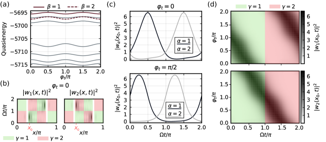
Figure 1: Temporal adiabatic pumping in a 2D time-space crystal with $s=2$ temporal cells and only one ($N=1$) spatial cell that consists of two spatial sites. The following values of parameters were used: $V_{{\rm S}}=7640$, $V_{{\rm L}}=2$, $\omega=410$, $s=2$, $\lambda_{{\rm S}}=100$, $\lambda_{{\rm L}}=40$ and $\varphi_{x}=0$. (a) Quasienergy levels $\varepsilon_{\beta}$ (see text for level numbering convention) of the Floquet Hamiltonian $\hat{{\cal H}}$ versus the adiabatic phase $\varphi_{t}$. (b) The Wannier functions $|w_{\alpha}(x,t)|^{2}$ at $\varphi_{t}=0$, represented by black regions. The shaded areas (green and pink) indicate the extent of the temporal cells ($\gamma=1,2$). (c) Wannier functions $|w_{\alpha}(x_{0},t)|^{2}$ (where $x_{0}=0.3\pi$) at $\varphi_{t}=0$ and $\varphi_{t}=\pi/2$. (d) Change of the Wannier functions $|w_{\alpha}(x_{0},t)|^{2}$ as $\varphi_{t}$ scans across a complete cycle of length $2\pi$. The green and pink shaded areas indicate the extent of the two temporal lattice cells ($\gamma=1,2$).

Since the perturbation $\xi_{{\rm S}}+\xi_{{\rm L}}$ is time-periodic, with the period $T=2\pi/\omega$ [see Eqs. (3)], we approach the problem by introducing the Floquet Hamiltonian $\hat{{\cal H}}=\hat{H}-\mathrm{i}\partial_{t}$ and solving the eigenvalue problem $\hat{{\cal H}}u_{n}(x,t)=\varepsilon_{n}u_{n}(x,t)$ [32, 33]. Here, $\varepsilon_{n}$ is the quasienergy of the $n$th eigenstate, while $u_{n}(x,t)$ is the corresponding Floquet mode that respects temporal periodicity of the perturbation, i.e. $u_{n}(x,t)=u_{n}(x,t+2\pi/\omega)$. A general solution of the Schrödinger equation can be represented as a superposition of states $\Psi_{n}(x,t)=\mathrm{e}^{-\mathrm{i}\varepsilon_{n}t}u_{n}(x,t).$ In our simulations we consider a finite number of spatial cells ($N=1$ or $N=2$) which leads to the Hamiltonian being defined on $x\in[0,N\pi)$, and we always assume periodic boundary conditions. All the details of the diagonalization procedure are covered in Appendix A.

III Simulations

In the following sections, we present the results of the simulations, starting with the Thouless pumping in time. Next, we consider pumping in space, which, however, is performed in a time-space crystal rather than a conventional space crystal. Finally, we study simultaneous pumping in both the temporal and the spatial dimensions.

A very helpful way to illustrate Thouless pumping is to show how Wannier states are transported with a change of an adiabatic parameter [34]. In our case we can observe pumping along temporal or spatial directions depending if we change $\varphi_{t}$ or $\varphi_{x}$. For pumping in time (space), we obtain a clear illustration when we analyze transport of Wannier states which are localized in a single site of temporal (spatial) lattice and are not necessarily localized along spatial (temporal) direction. To construct such Wannier states, we will choose Floquet states which correspond to quasi-energy levels with different temporal (spatial) index. Note that choosing Floquet states from a given band, one obtains Wannier states which live in the corresponding Hilbert subspace and which are uncoupled from states belonging to any other bands.

III.1 Thouless pumping in time

We begin the analysis by considering time-pumping in a system of a single spatial cell ($N=1$) which contains two sites originating from the double-well structure of the spatial potential. The relevant part of the quasienergy spectrum of $\hat{{\cal H}}$ is shown in Fig. 1(a). The figure displays the changes of the quasienergy levels in the course of the adiabatic pumping in the temporal dimension — the temporal phase $\varphi_{t}$ is varied while keeping $\varphi_{x}=0$. We interpret the obtained quasienergy spectrum as follows. In the limit of an infinite spatial crystal, the energy spectrum of $\hat{h}$ features series of bands separated by large gaps. Because of the double-well structure of each cell of the potential, each band consists of two sub-bands (a higher and a lower one), separated by a small gap, of order $V_{{\rm L}}$ at $\varphi_{x}=0$. Thus, each two consecutive levels in Fig. 1(a) correspond, respectively, to the higher and the lower sub-bands of a certain spatial band. For example, the two topmost levels in Fig. 1(a) correspond to the sub-bands of the spatial band number 25 (counting from the lowest); the spatial potential supports 28 clearly formed bands in total with the chosen parameter values. From the time-crystalline structure perspective, we associate the four topmost levels in Fig. 1(a) with the first temporal band, and the lower four levels with the second. Note that it is natural to assign the lowest band number to the temporal band whose quasienergy is largest: a particle confined in the temporal lattice is parameterized by the effective mass which is negative (see Appendix B) and its energy spectrum is thus bounded from above. To distinguish the quasienergy levels constituting the first temporal band, we introduce an index $\beta$. We assign the same index $\beta$ to all the levels corresponding to the same spatial band: we assign $\beta=1$ to the two topmost levels in Fig. 1(a) and $\beta=2$ to the next two.

Analysis of the pumping process may be conveniently approached by constructing the Wannier functions [35, 36, 37, 34], which are spatially localized superpositions of the relevant Floquet modes: $w_{\alpha}(x,t)=\sum_{\beta=1}^{2}d_{\beta}^{(\alpha)}u_{\beta}(x,t)$, where the coefficients $d_{\beta}^{(\alpha)}$ are found by diagonalizing the position operator $\mathrm{e}^{2\mathrm{i}x/N}$ (see Appendix A). We will only consider the quasienergy levels of the first temporal band. This is justified by assuming that the gap between the first and the second bands is large enough so that particles loaded into the first band stay there throughout the pumping cycle. Furthermore, since we are now considering pumping in the temporal direction only, we can restrict our attention to a single site (out of two) of the spatial lattice. To obtain Wannier functions that are localized in the same spatial site, we have to mix the spatial energy levels corresponding either to the higher spatial sub-bands or to the lower ones. We choose to mix the levels of the higher spatial sub-bands by mixing the two modes $\beta=1,2$ whose quasienergy levels are highlighted in Fig. 1(a). Mixing the other pair of levels (from the first temporal band) leads to analogous results and corresponds to a particle occupying the other site of the spatial lattice.

The obtained Wannier functions $w_{1}(x,t)$ and $w_{2}(x,t)$ are shown in Fig. 1(b) at $\varphi_{t}=0$ where they are represented by black regions. In the present case we consider only one spatial cell; the two sites of this cell span the regions $x\in[0,\pi/4)\cup[3\pi/4,\pi)$ and $x\in[\pi/4,3\pi/4)$ — note that we assume periodic boundary conditions in space. The sites are separated by white gaps in Fig. 1(b). Each of the spatial sites contains $s=2$ temporal cells, which we will number with the index $\gamma=1,2$ and which are indicated by shaded green and pink areas. We adopt the convention that the region of time-space which is occupied by $w_{1}$ at $\varphi_{t}=0$ belongs to the first temporal cell [$\gamma=1$, green shading in Fig. 1(b)], while the region occupied by $w_{2}$ belongs to the second temporal cell [$\gamma=2$, pink shading in Fig. 1(b)]. Note that at a different value of $\varphi_{t}$, the state $w_{1}$ may spread over both temporal cells or even transition to cell $\gamma=2$, and similarly for $w_{2}$. As illustrated in Fig. 1(b), the Wannier functions cycle in time between the two turning points of the spatial site they are confined to, akin to classical pendula.

In space crystals we are interested in periodic distribution of particles in space at a fixed moment of time (i.e. the moment of the detection). Switching from space to time crystals, the roles of space and time are exchanged. That is, we fix position in space and ask if the probability for the detection of particles at this fixed space-point changes periodically in time [3]. To understand the emergence of a time-crystalline structure in the system analyzed here, let us consider placing a detector close to the left (say) classical turning point $x_{0}$ of the spatial lattice site under consideration. We take $x_{0}=0.3\pi$ for the chosen energy regime, as indicated in Fig. 1(b). As shown in Fig. 1(c) depicting the time-periodic Wannier functions $w_{\alpha}(x_{0},t)$ at $\varphi_{t}=0$, in the time intervals $(\Omega t\bmod 2\pi)\in[0,\pi)$ the detector will most likely be registering the particle whose wave function is $w_{1}(x_{0},t)$. Meanwhile, in the intervals $(\Omega t\bmod 2\pi)\in[\pi,2\pi)$ the detector will most likely be registering the particle whose wave function is $w_{2}(x_{0},t)$. The two time intervals can be considered to divide the time axis into cells, allowing one to introduce the notion of a time-crystalline structure. In the present case, the temporal dimension of the crystalline structure is $2\pi/\Omega$, and the crystal is periodic in this dimension, i.e. periodic boundary conditions in time are imposed. The lower panel of Fig. 1(c) demonstrates additionally that at a different value of the phase, $\varphi_{t}=\pi/2$, the Wannier functions are shifted and they are delocalized over both cells of the temporal lattice.

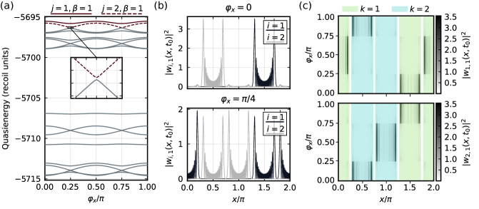
Figure 2: Spatial adiabatic pumping in a 2D time-space crystal with $s=2$ temporal cells and $N=2$ spatial cells.. The same values of parameters were used as in Fig. 1 except that $\varphi_{t}=0$, while $\varphi_{x}$ is varied. (a) Quasienergy levels $\varepsilon_{j,\beta}$ of the Floquet Hamiltonian $\hat{{\cal H}}$ versus the adiabatic phase $\varphi_{x}$. (b) Wannier functions $|w_{i,1}(x,t_{0})|^{2}$ (where $t_{0}=\pi/2\Omega$) at $\varphi_{x}=0$ and $\varphi_{x}=\pi/4$. (c) Changes of the Wannier functions $|w_{i,1}(x,t_{0})|^{2}$ as $\varphi_{x}$ scans across a complete cycle of length $\pi$. The cyan and green shaded areas indicate the extent of the two spatial lattice cells ($k=1,2$), each consisting of two sites separated by unshaded regions.

Having introduced the concept of a crystalline structure in time, we now turn to the Thouless pumping in the temporal dimension. To this end, we calculate the Wannier functions repeatedly as the phase $\varphi_{t}$ is varied and produce the plots of $w_{1}(x_{0},t)$ and $w_{2}(x_{0},t)$ for each value of $\varphi_{t}$, as shown in Fig. 1(d). We can clearly see that $w_{1}$ is being pumped from cell $\gamma=1$ to cell $\gamma=2$ as the temporal phase $\varphi_{t}$ is varied from 0 to $2\pi$. At the same time, state $w_{2}$ adiabatically transitions from cell 2 to cell 1. To observe the pumping experimentally, one has to prepare a particle in, e.g., the state $w_{1}(x,t)$ and place a detector at $x_{0}$. Initially, the detector will most probably be detecting the particle in the time intervals $(\Omega t\bmod 2\pi)\in[0,\pi)$, whereas after a pumping cycle is complete the detector will be clicking in the time intervals $(\Omega t\bmod 2\pi)\in[\pi,2\pi)$. We note in passing that one can “invert” the pumping direction by letting $\varphi_{t}$ vary from 0 to $-2\pi$, just as is possible in the case of the adiabatic pumping in real space.

III.2 Thouless pumping in space

Now let us analyze spatial-only pumping in a 2D time-space crystalline structure consisting of $N=2$ spatial cells (and $s=2$ temporal cells) with periodic boundary conditions. Doubling the number of spatial cells leads to a twice greater number of Floquet quasienergy levels compared to the case of $N=1$, as shown in Fig. 2(a). The physical origin of the levels is the same as in the preceding discussion, and it is now immediately apparent which levels arise from the higher and the lower spatial sub-bands. The gap between the sub-bands is the smallest (but non-vanishing) at $\varphi_{x}=\pi/4$ and $\varphi_{x}=3\pi/4$ since all wells of the spatial potential are of equal depth at these phases. Once the quasienergy spectrum is obtained, we again switch to the Wannier representation, this time introducing an additional spatial index $j$ to number the Floquet modes and $i$ to number the Wannier functions: $w_{i,\alpha=1}(x,t)=\sum_{j=1}^{2}d_{j}^{(i)}u_{j,\beta=1}(x,t)$. Since we are interested in the spatial pumping, we mix the Floquet modes bearing the same temporal index $\beta=1$ so that the obtained Wannier functions come out delocalized over the entire temporal lattice structure, simplifying the analysis. The delocalization in the temporal dimension and localization in spatial dimension means physically that the particle, being confined to a single spatial site, can be detected with equal probabilities at both turning points, this being true at all times. This contrasts the situation in Sec. III A, where, at any given time, a particle could be detected at one turning point with a higher probability than at the other, and based on this probability we could speak of the particle occupying a specific temporal cell. Note that the eigenstates of $\mathrm{e}^{2\mathrm{i}x/N}$ are always strongly localized in certain sites of the spatial lattice, and so are the Wannier functions $w_{i,\alpha}(x,t)$, at all $t$. The latter is only violated at values of $\varphi_{x}$ close to $(2n+1)\pi/4$, $n\in\mathbb{Z}$, when the depths of all the wells of the potential become equal, leading to the Wannier functions spreading over two adjacent sites. The temporal dependence of $w_{i,\alpha}(x,t)$, on the other hand, is dictated by the temporal dependencies of the modes $u_{j,\beta}(x,t)$ that are being mixed.

The relevant quasienergy levels are highlighted in Fig. 2(a). Their indices are $(j=1,\beta=1)$ and $(j=2,\beta=1)$ corresponding to them occupying two different spatial cells. To analyze the pumping, we study the states $w_{1,1}(x,t_{0})$ and $w_{2,1}(x,t_{0})$ at a fixed detection moment $t_{0}=\pi/2\Omega$. Figure 2(b) illustrates that, at $\varphi_{x}=0$, each of these states is localized in a single site of the spatial lattice, while at $\varphi_{x}=\pi/4$ they occupy two sites in the process. We number the states and the cells of the spatial lattice such that $w_{1,1}$ occupies spatial cell $k=1$, while $w_{2,1}$ occupies spatial cell $k=2$ at the beginning of the pumping cycle (at $\varphi_{x}=0$), as shown in Fig. 2(c). In the figure, the cyan and green shaded areas indicate the spatial extent of the spatial lattice cells, with the sites of the cells separated by unshaded gaps corresponding to the positions of the barriers of the spatial potential. In the end of the cycle, the Wannier states end up in a cell different from the starting one, confirming that pumping does take place. It is apparent that the states remain almost insensitive to the change of the potential and are transported to a neighboring site abruptly. However, the lower panel of Fig. 2(b) demonstrates that the transfer does not happen instantaneously, but rather proceeds via a stage when the Wannier states occupy both sites.

We remark that constructing the Wannier functions using the Floquet modes corresponding to the top third and fourth levels in Fig. 2(a) leads to pumping in the opposite direction around the circular $x$-axis (not shown). This is to be expected since those energy levels correspond to the lower spatial sub-bands, while the above results concern pumping in the higher sub-bands [34].

III.3 2D Thouless pumping

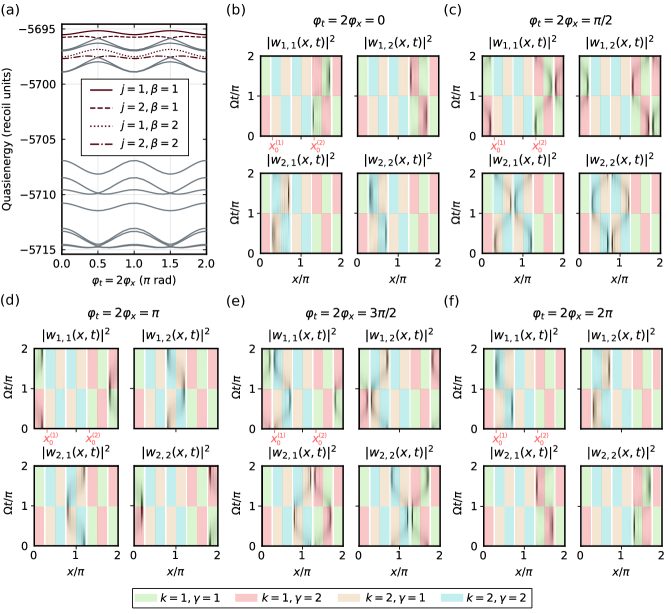
Figure 3: Simultaneous temporal and spatial adiabatic pumping in a 2D time-space crystal. The same values of parameters were used as in Fig. 1 except that both $\varphi_{t}$ and $\varphi_{x}$ are varied. (a) Quasienergy levels $\varepsilon_{j,\beta}$ of the Floquet Hamiltonian $\hat{{\cal H}}$ versus the adiabatic phase $\varphi_{t}=2\varphi_{x}$. (b)–(f) The Wannier functions at $\varphi_{t}=2\varphi_{x}=0,\pi/2,\pi,3\pi/2,2\pi$. The probability densities $|w_{i,\alpha}(x,t)|^{2}$ are represented by black regions, while the shaded areas indicate the extent of the spatial ($k=1,2$) and temporal ($\gamma=1,2$) cells. In top-left panels in (b)–(f), $x_{0}^{(1)}$ and $x_{0}^{(2)}$ indicate the locations of two detectors, see text.

We are now ready to discuss the simultaneous temporal and spatial adiabatic pumping, demonstrated in Fig. 3 for the case $N=s=2$. The adiabatic phases are varied along the trajectory $\varphi_{t}=2\varphi_{x}$ from $\varphi_{t}=0$ to $\varphi_{t}=2\pi$ so that a complete pumping cycle is performed both in the temporal and in the spatial dimensions. The obtained Floquet quasienergy spectrum is shown in Fig. 3(a), where the legend indicates the quasienergy levels corresponding to the modes that we mix when constructing the Wannier states. The relevant modes are those of the first temporal band, among which we select those corresponding to the higher spatial sub-bands. As discussed in Sec. III B, this selection allows us to focus on the Wannier states that are transported in space to the right during the pumping process. The remaining four levels of the first temporal band constitute the Wannier functions that are being pumped to the left in space. The constructed states are expressed as $w_{i,\alpha}(x,t)=\sum_{j,\beta}d_{j,\beta}^{(i,\alpha)}u_{j,\beta}(x,t)$ and are obtained as above, by diagonalizing the position operator $\mathrm{e}^{2\mathrm{i}x/N}$. Contrary to the preceding analysis, we no longer restrict our attention to a certain position $x_{0}$ or a certain detection time $t_{0}$, but rather study the two-dimensional maps of the Wannier functions $w_{i,\alpha}(x,t)$. The four Wannier states are shown in Figs. 3(b)–(f) at various values of the adiabatic phases, with the shaded areas dividing the whole time-space into temporal and spatial cells. The states and the cells are numbered so that initially (at $\varphi_{t}=2\varphi_{x}=0$) the Wannier state indices $(i,\alpha)$ coincide with the spatial and temporal cell numbers $(k,\gamma)$. In each of the panels (b)–(f), four sites are left unoccupied by any Wannier functions — these would be occupied by the Wannier functions constructed using the states of the lower spatial sub-bands, i.e. the Floquet modes corresponding to the top four unhighlighted quasienergy levels in Fig. 3(a). We note in passing that the two Wannier functions constructed in Sec. III B using the states corresponding to only the two upper quasienergy levels appear as the sums $w_{1,1}+w_{1,2}$ and $w_{2,1}+w_{2,2}$, where $w_{i,\alpha}$ are the functions displayed in Figs. 3(b)–(f). Such sums exhibit spatial, but not temporal localization.

Turning to the pumping process, in Fig. 3(c) we see the Wannier states are transported to the neighboring spatial site (to the right) as a result of the spatial pumping, while the temporal pumping causes the states to slide down the temporal axis. At $\varphi_{t}=2\varphi_{x}=\pi$ [see Fig. 3(d)], the spatial transition is complete, whereas the time dependence of the functions is such that the functions occupy both temporal cells. Next, at $\varphi_{t}=2\varphi_{x}=3\pi/2$ [see Fig. 3(e)], the states are shown in the middle of the second spatial transition, which is completed at $\varphi_{t}=2\varphi_{x}=2\pi$ [see Fig. 3(f)]. Comparing Figs. 3(b) and 3(f), it is apparent that as a result of the pumping each state $w_{i,\alpha}$ has transitioned from cell $(i,\alpha)$ to cell $(i+1\mod N,\ \alpha+1\mod s)$.

Let us now give an interpretation of these results. Consider two detectors, one placed at $x_{0}^{(1)}=0.3\pi$ and the other one at $x_{0}^{(2)}=1.3\pi$, and a particle loaded initially into the system in the state $w_{1,1}$. At $\varphi_{t}=2\varphi_{x}=0$, most probably a detector placed at $x_{0}^{(2)}$ will be detecting the particle in the time intervals $(\Omega t\bmod 2\pi)\in[0,\pi)$, corresponding to the particle occupying the first spatial and the first temporal cells [see Fig. 3(b)]. In the end of the pumping cycle ($\varphi_{t}=2\varphi_{x}=2\pi$), the particle will most probably appear in the time intervals $(\Omega t\bmod 2\pi)\in[\pi,2\pi)$ on a detector placed at $x_{0}^{(1)}$, corresponding to the particle occupying the second spatial and the second temporal cells.

IV Conclusions

Summarizing our work, we have shown that the quasienergy spectrum of a resonantly driven optical lattice may be interpreted as that of a crystal-like structure with the time playing the role of an additional coordinate. Using this analogy, we studied adiabatic variation of the driving protocol and demonstrated that it leads to a change of system dynamics that is a manifestation of the Thouless pumping in the temporal dimension. Finally, we have illustrated simultaneous adiabatic pumping in both spatial and temporal directions.

Appendix A: Diagonalization of Floquet Hamiltonian

In this section, we discuss the diagonalization of the Floquet Hamiltonian

$$\hat{{\cal H}}=\hat{h}-\mathrm{i}\frac{\partial}{\partial t}+\xi_{{\rm S}}+\xi_{{\rm L}},$$ (A1)

where $\hat{h}$ is defined in Eq. (2), while $\xi_{{\rm S}}$ and $\xi_{{\rm L}}$ are given in Eqs. (3).

In order to solve the eigenvalue problem

$$\hat{{\cal H}}u_{n}(x,t)=\varepsilon_{n}u_{n}(x,t),$$ (A2)

we first numerically obtain the eigenstates of $\hat{h}$ in the basis of plane waves $\left\langle x|j\right\rangle=\mathrm{e}^{\mathrm{i}\frac{2j}{N}x}/\sqrt{N\pi}$ orthonoromal on $x\in[0,N\pi)$, where $N$ is the number of spatial cells. The sought eigenstates fulfill

$$\hat{h}\psi_{m}(x)=\epsilon_{m}\psi_{m}(x),$$ (A3)

are written as

$$\psi_{m}(x)=\frac{1}{\sqrt{N\pi}}\sum_{j=-\infty}^{\infty}c_{j}^{(m)}\,\mathrm{e}^{\mathrm{i}\frac{2j}{N}x},$$ (A4)

and the coefficients $c_{j}^{(m)}$ that express the solution in the $m$th energy band are obtained by diagonalizing the matrix

$$\begin{split}\left\langle j^{\prime}\right|h\left|j\right\rangle&=\left[\left(\frac{2j}{N}\right)^{2}+\frac{V_{{\rm S}}+V_{{\rm L}}}{2}\right]\delta_{j^{\prime},j}\\ &+\frac{V_{{\rm S}}}{4}(\delta_{j^{\prime},j+2N}+\delta_{j^{\prime},j-2N})\\ &+\frac{V_{{\rm L}}}{4}(\mathrm{e}^{2\mathrm{i}\varphi_{x}}\delta_{j^{\prime},j+N}+\mathrm{e}^{-2\mathrm{i}\varphi_{x}}\delta_{j^{\prime},j-N}).\end{split}$$ (A5)

Once we have the eigenstates of the unperturbed Hamiltonian, an additional transformation to the rotating frame provides a suitable basis consisting of functions

$$\psi^{\prime}_{m}(x,t)=\mathrm{e}^{-\mathrm{i}\nu(m)\omega t/s}\psi_{m}(x).$$ (A6)

Here, the function $\nu(m)=\lceil m/2N\rceil$ (where $\lceil\cdots\rceil$ is the ceiling operation) transforms the level numbers $m=1,2,3,4,5,6,\ldots$ into band indices

$$\nu=\underset{2N\text{ times}}{\underbrace{1,\ldots,1}},\underset{2N\text{ times}}{\underbrace{2,\ldots,2}},\underset{2N\text{ times}}{\underbrace{3,\ldots,3}},\underset{2N\text{ times}}{\underbrace{4,\ldots,4}},\ldots$$ (A7)

Note that this labeling is correct when the sites of a potential cell are not too asymmetric for all $\varphi_{x}$ — otherwise one has to examine how to properly label the unperturbed eigenstates so that the unitary transformation (A6) corresponds to the canonical transformation to the moving frame (see Appendix B). In practice, we have to keep $V_{{\rm L}}$ small enough so that the difference of depths of the potential wells in each cell is always smaller than the gaps between the energy bands.

We now calculate the matrix elements of $\hat{{\cal H}}$. For the diagonal part, we have

$$\left\langle\psi^{\prime}_{m^{\prime}}\right|\left(\hat{h}-\mathrm{i}\frac{\partial}{\partial t}\right)\left|\psi^{\prime}_{m}\right\rangle=\left[\epsilon_{m}-\frac{\nu(m)\omega}{s}\right]\delta_{m^{\prime},m}.$$ (A8)

For the long perturbation, we obtain

$$\begin{split}&\left\langle\psi^{\prime}_{m^{\prime}}\right|\xi_{{\rm L}}\left|\psi^{\prime}_{m}\right\rangle=\lambda_{{\rm L}}\\ &\qquad\times\cos(\omega t+\varphi_{t})\,\mathrm{e}^{-\mathrm{i}(\omega/s)[\nu(m)-\nu(m^{\prime})]t}\\ &\qquad\times\sum_{j,j^{\prime}}c_{j^{\prime}}^{(m^{\prime})*}c_{j}^{(m)}\int_{0}^{\pi}\frac{\mathrm{d}x}{\pi}{\cal Q}_{{\rm L}}(x)\,\mathrm{e}^{\mathrm{i}(2j-2j^{\prime})x},\end{split}$$ (A9)

where ${\cal Q}_{{\rm L}}$ is the spatial part of $\xi_{{\rm L}}$, see Eqs. (3). Applying the secular approximation, we replace

$$\cos(\omega t+\varphi_{t})\,\mathrm{e}^{-\mathrm{i}(\omega/s)[\nu(m)-\nu(m^{\prime})]t}$$ (A10)

with its time-independent contribution

$$\tfrac{1}{2}(\mathrm{e}^{\mathrm{i}\varphi_{t}}\delta_{\nu^{\prime}+s,\nu}+\mathrm{e}^{-\mathrm{i}\varphi_{t}}\delta_{\nu^{\prime}-s,\nu}),$$ (A11)

where $\nu^{\prime}\equiv\nu(m^{\prime})$. With our choice ${\cal Q}_{{\rm L}}(x)=\cos^{2}(2x)$, we finally obtain

$$\left\langle\psi^{\prime}_{m^{\prime}}\right|\xi_{{\rm L}}\left|\psi^{\prime}_{m}\right\rangle=\frac{\lambda_{{\rm L}}}{2}(\mathrm{e}^{\mathrm{i}\varphi_{t}}\delta_{\nu^{\prime}+s,\nu}+\mathrm{e}^{-\mathrm{i}\varphi_{t}}\delta_{\nu^{\prime}-s,\nu})\\ \times\frac{1}{4}\sum_{j=-\infty}^{\infty}c_{j}^{(m)}(2c_{j}^{(m^{\prime})*}+c_{j+2}^{(m^{\prime})*}+c_{j-2}^{(m^{\prime})*}).$$ (A12)

Similarly, using ${\cal Q}_{{\rm S}}(x)=\sin^{2}(2x)$, the matrix elements of the short perturbation follow as

$$\left\langle\psi^{\prime}_{m^{\prime}}\right|\xi_{{\rm S}}\left|\psi^{\prime}_{m}\right\rangle=\frac{\lambda_{{\rm S}}}{2}(\mathrm{e}^{\mathrm{i}\varphi_{t}}\delta_{\nu^{\prime}+2s,\nu}+\mathrm{e}^{-\mathrm{i}\varphi_{t}}\delta_{\nu^{\prime}-2s,\nu})\\ \times\frac{1}{4}\sum_{j=-\infty}^{\infty}c_{j}^{(m)}(2c_{j}^{(m^{\prime})*}-c_{j+2}^{(m^{\prime})*}-c_{j-2}^{(m^{\prime})*}).$$ (A13)

Once the eigenfunctions $u_{n}(x,t)=\sum_{m}b_{m}^{(n)}\psi^{\prime}_{m}(x,t)$ are found, the Wannier functions are constructed by diagonalizing the periodic position operator $\mathrm{e}^{\mathrm{i}\frac{2}{N}x}$ [34, 38], whose matrix elements result as

$$\begin{split}\left\langle u_{n^{\prime}}\right|\mathrm{e}^{\mathrm{i}\frac{2}{N}x}\left|u_{n}\right\rangle&=\sum_{j=-\infty}^{\infty}\sum_{m,m^{\prime}}b_{m^{\prime}}^{(n^{\prime})*}b_{m}^{(n)}c_{j+1}^{(m^{\prime})*}c_{j}^{(m)}\\ &\qquad\times\mathrm{e}^{\mathrm{i}[\nu(m^{\prime})-\nu(m)]\omega t/s}.\end{split}$$ (A14)

The diagonalization is performed at a chosen time moment $t$. The obtained coefficients $d_{n}^{(k)}$ are used to express the Wannier states as

$$w_{k}(x,t)=\sum_{n}d_{n}^{(k)}u_{n}(x,t).$$ (A15)

Note that the position operator is constructed using only the relevant subspace of eigenvectors $\left|u_{n}\right\rangle$ that we select based on our interpretation of the quasienergy spectrum, as discussed in the main text. Subsequent renumbering of these eigenvectors and the Wannier states using a pair of indices $(i,\alpha)$ is likewise conventional.

All calculations have been performed using a number of software packages [39, 40, 41, 42, 43] written in the Julia programming language [44].

Appendix B: Quasiclassical analysis of the temporal Thouless pumping

It is instructive to perform an analysis of a one-dimensional time crystal, whereby a particle is confined to a single potential well and the spatial periodicity plays no role. Rather than using the Floquet theory, we can consider our model Hamiltonian

$$H(p_{x},x,t)=h(p_{x},x|\varphi_{x})+\xi_{{\rm S}}(x,t)+\xi_{{\rm L}}(x,t|\varphi_{t})$$ (B1)

as a classical entity and use the action–angle representation of the unperturbed Hamiltonian $h(I)$, with the action $I$ and angle $\theta\in[0,2\pi)$ constituting a pair of canonical variables [45]. Specifically, the action variable is defined for a one-dimensional time-independent Hamiltonian [$h(p_{x},x|\varphi_{x})$ in our case] as the integral of momentum along a periodic orbit

$$I=\frac{1}{2\pi}\oint p_{x}\,\mathrm{d}x.$$ (B2)

The angle $\theta$ is the position variable of a particle on a periodic trajectory that changes uniformly in time, $\theta(t)=\Omega t+\theta(0)$, where the frequency of the periodic motion $\Omega=\partial h(I)/\partial I$. The periodic motion of a classical particle confined to a single lattice site of the potential in $h$ is represented in the $(I,\theta)$ phase space by straight lines $I(\theta)={\rm const}$ when no time-dependent perturbation is present. The perturbation causes formation of resonant islands that contain closed orbits in the vicinity of the resonant value of action $I_{s}$ such that $\Omega=[\partial h(I)/\partial I]\big{|}_{I_{s}}=\omega/s$ where $s$ in an integer [33]. Analysis of the motion may be simplified by transitioning to the frame moving along the resonant orbit and applying the secular approximation, whereby the oscillatory terms of the Hamiltonian are dropped. We give all the details of this calculation below.

Setting $\varphi_{x}=0$ and performing a transformation to the action–angle variables, we obtain

$$\begin{split}H(I,\theta,t)&=h(I)\\ &+\lambda_{{\rm S}}\cos(2\omega t){\cal Q}_{{\rm S}}(I,\theta)\\ &+\lambda_{{\rm L}}\cos(\omega t+\varphi_{t}){\cal Q}_{{\rm L}}(I,\theta),\end{split}$$ (B3)

where ${\cal Q}_{{\rm S}}(x)=\sin^{2}(2x)$ and ${\cal Q}_{{\rm L}}(x)=\cos^{2}(2x)$ — we have chosen different functions for ${\cal Q}_{{\rm S}}(x)$ and ${\cal Q}_{{\rm L}}(x)$ but one can also choose $\sin(2x)$ [or $\cos(2x)$] for both of them. The spatial Hamiltonian $h(I)$ does not depend on $\theta$, and the $\theta$-dependencies of the perturbations can be represented as Fourier series

$${\cal Q}_{{\rm S}/{\rm L}}(I,\theta)=\sum_{m=-\infty}^{\infty}{\cal Q}_{{\rm S}/{\rm L}}^{(m)}(I)\,\mathrm{e}^{\mathrm{i}m\theta}.$$ (B4)

We choose our working point in the vicinity of a certain resonant trajectory corresponding to a given value of the action $I_{s}$ and the corresponding intrinsic frequency $\Omega$. Switching to the rotating frame according to $\Theta=\theta-\Omega t$ and averaging out the rapidly oscillating terms, we express the long perturbation as

$$\xi_{{\rm L}}=\frac{1}{2}\lambda_{{\rm L}}\left[{\cal Q}_{{\rm L}}^{(s)}(I_{s})\,\mathrm{e}^{\mathrm{i}(\varphi_{t}-s\Theta)}+{\rm c.c.}\right].$$ (B5)

Writing the complex number ${\cal Q}_{{\rm L}}^{(s)}(I_{s})$ in the polar form

$${\cal Q}_{{\rm L}}^{(s)}(I_{s})\equiv A_{{\rm L}}\,\mathrm{e}^{\mathrm{i}\chi_{{\rm L}}},$$ (B6)

we cast this result into

$$\xi_{{\rm L}}=\lambda_{{\rm L}}A_{{\rm L}}\cos(s\Theta-\chi_{{\rm L}}-\varphi_{t}).$$ (B7)

In complete analogy, the short perturbation is written as

$$\xi_{{\rm S}}=\lambda_{{\rm S}}A_{{\rm S}}\cos(2s\Theta-\chi_{{\rm S}}),$$ (B8)

where $A_{{\rm S}}\,\mathrm{e}^{\mathrm{i}\chi_{S}}$ is the polar form of ${\cal Q}_{S}^{(2s)}(I_{s})$.

We also expand $h(I)$ around $I_{s}$ to the second order in $I$,

$$h(I)=h(I_{s})+(I-I_{s})\Omega+\frac{1}{2}h^{\prime\prime}(I_{s})(I-I_{s})^{2}.$$ (B9)

Noting also that the time-dependent canonical transformation introduces an additional term $-I\Omega$, we finally derive the effective Hamiltonian

$$\begin{split}H_{{\rm eff}}&=[h(I_{s})-\Omega I_{s}]+\frac{P^{2}}{2M}\\ &+\lambda_{{\rm S}}A_{{\rm S}}\cos(2s\Theta-\chi_{{\rm S}})\\ &+\lambda_{{\rm L}}A_{{\rm L}}\cos(s\Theta-\chi_{{\rm L}}-\varphi_{t}),\end{split}$$ (B10)

with $P\equiv I-I_{s}$. Here we have also defined the “effective mass” $M=1/h^{\prime\prime}(I_{s})$, which is negative. The last two lines of Eq. (B10) represent a periodic potential in the moving frame. For $s=2$, we obtain a lattice of two elementary cells, each consisting of two sites arising from the double-well structure.

In order to verify the validity of the secular approximation, we produce a map of the motion of a particle in the $(I,\theta)$ phase-space governed by the secular effective Hamiltonian (B10), as shown in Fig. B1, left panel. The right panel displays the map obtained by integrating the exact equations of motion resulting from the Hamiltonian (B3) and by registering particle’s coordinates stroboscopically at the intervals of the lattice driving period. Such a stroboscopic, rather than continuous, picture precisely corresponds to the secular approximation, which only provides the information on the dynamics averaged over the driving period. Comparing the two plots in Fig. B1, we conclude that the resonant islands where the quantum states we are interested in will be located (in the semiclassical sense) are well reproduced in the exact picture, and hence that the secular approximation is valid for the considered strength of the perturbation (i.e. values of $\lambda_{{\rm S}}$ and $\lambda_{{\rm L}}$).

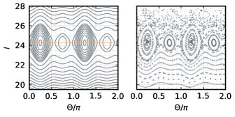
Figure B1: Phase-space maps of the particle motion governed by the secular effective Hamiltonian (B10) (left panel) and the exact Hamiltonian (B3) (right panel). The yellow line in the left panel indicates the working point $I_{s}=24.3$. The map in the right panel was generated by numerically integrating the classical equations of motion resulting from the exact Hamiltonian (B3) and registering particle’s position $(\theta,I)$ stroboscopically at the intervals of the lattice driving period. The same values of parameters were used as in Fig. 1.

We are now in position to quantize the classical effective Hamiltonian (B10) by changing $\Theta\to\hat{\Theta}=\Theta$ and $P\to\hat{P}=-\mathrm{i}\partial/\partial\Theta$:

$$\begin{split}\hat{H}_{{\rm eff}}&=[h(I_{s})-\Omega I_{s}]-\frac{1}{2M}\frac{\partial^{2}}{\partial\Theta^{2}}\\ &+\lambda_{{\rm S}}A_{{\rm S}}\cos(2s\Theta-\chi_{{\rm S}})\\ &+\lambda_{{\rm L}}A_{{\rm L}}\cos(s\Theta-\chi_{{\rm L}}-\varphi_{t}).\end{split}$$ (B11)

This form of the Hamiltonian is particularly convenient since it features an explicit expression for the temporal potential, which is not the case for Eq. (1). In complete analogy with conventional space crystals, we may consider the limit of a large number of cells, $s\gg 1$ (while $\Theta\in[0,2\pi)$). In that case, the eigenstates of Hamiltonian (B11) are Bloch waves given by $\psi_{n,{\cal K}}(\Theta)=\mathrm{e}^{\mathrm{i}{\cal K}\Theta}u_{n,{\cal K}}(\Theta)$, where ${\cal K}$ is the time-quasimomentum and $u_{n,{\cal K}}(\Theta)=u_{n,{\cal K}}(\Theta+2\pi/s)$ are cell-periodic functions [17]. Relevant for the Thouless pumping, one may introduce the Berry curvature related to the $n$th energy band as $\Omega_{n}(\varphi_{t},{\cal K})=\mathrm{i}(\left\langle\partial_{\varphi_{t}}u_{n}|\partial_{{\cal K}}u_{n}\right\rangle-\left\langle\partial_{{\cal K}}u_{n}|\partial_{\varphi_{t}}u_{n}\right\rangle)$ and the corresponding first Chern number [46, 28, 27]

$$\nu_{n}=\frac{1}{2\pi}\int_{{\rm BZ}}\mathrm{d}{\cal K}\intop_{0}^{2\pi}\mathrm{d}\varphi_{t}\,\Omega_{n}(\varphi_{t},{\cal K}),$$ (B12)

where we integrate over a Brillouin zone in ${\cal K}$-space as the phase $\varphi_{t}$ completes a pumping cycle.

Numerical diagonalization of (B11) is straightforward: in order to solve the eigenvalue problem

$$\hat{H}_{{\rm eff}}\psi_{\beta}(\Theta)=E_{\beta}\psi_{\beta}(\Theta)$$ (B13)

under periodic boundary conditions, $\psi_{\beta}(\Theta)=\psi_{\beta}(\Theta+2\pi)$, we expand the eigenfunctions in the basis of plane waves $\left\langle\Theta|j\right\rangle=\mathrm{e}^{\mathrm{i}j\Theta}/\sqrt{2\pi},$ $j\in\mathbb{Z}$, which are orthonoromal on $\Theta\in[0,2\pi)$:

$$\psi_{\beta}(\Theta)=\frac{1}{\sqrt{2\pi}}\sum_{j=-\infty}^{\infty}c_{j}^{(\beta)}\,\mathrm{e}^{\mathrm{i}j\Theta}.$$ (B14)

This leads to the following matrix elements:

$$\left\langle j^{\prime}\right|\hat{H}_{{\rm eff}}\left|j\right\rangle =\left[h(I_{s})-\Omega I_{s}+\frac{j^{2}}{2M}\right]\delta_{j^{\prime},j}$$

$$+\frac{\lambda_{{\rm S}}A_{{\rm S}}}{2}(\delta_{j^{\prime},j+2s}\,\mathrm{e}^{-\mathrm{i}\chi_{{\rm S}}}+\delta_{j^{\prime},j-2s}\,\mathrm{e}^{\mathrm{i}\chi_{{\rm S}}})$$ (B15)

$$+\frac{\lambda_{{\rm L}}A_{{\rm L}}}{2}(\delta_{j^{\prime},j+s}\,\mathrm{e}^{-\mathrm{i}(\chi_{{\rm L}}+\varphi_{t})}+\delta_{j^{\prime},j-s}\,\mathrm{e}^{\mathrm{i}(\chi_{{\rm L}}+\varphi_{t})}).$$

The final ingredient needed for the analysis is the Wannier functions, which are localized superpositions of the stationary states of $\hat{H}_{{\rm eff}}$. They may be found by diagonalizing the position operator. In the case of a periodic system, we take this operator in the form $\mathrm{e}^{\mathrm{i}\Theta}$ [38, 34]. Its matrix elements follow as

$$\left\langle\psi_{\beta^{\prime}}\right|\mathrm{e}^{\mathrm{i}\Theta}\left|\psi_{\beta}\right\rangle=\sum_{j=-\infty}^{\infty}c_{j+1}^{(\beta^{\prime})*}c_{j}^{(\beta)}.$$ (B16)

Numerical diagonalization of this operator yields the coefficients $d_{\beta}^{(\alpha)}$ that allow us to express the Wannier states as

$$w_{\alpha}(\Theta)=\sum_{\beta}d_{\beta}^{(\alpha)}\psi_{\beta}(\Theta).$$ (B17)

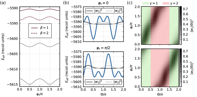
Figure B2: Adiabatic pumping in a two-cell time crystal simulated based on the quasiclassical approach. The same values of parameters were used as in Fig. 1. (a) Energy levels $E_{\beta}$ of quantized effective Hamiltonian (B11) versus the adiabatic phase $\varphi_{t}$. (b) Wannier functions $|w_{\alpha}(\Theta)|^{2}$ superimposed on the effective potential (blue curves) $U_{{\rm eff}}=H_{{\rm eff}}-P^{2}/2M$ at $\varphi_{t}=0$ and $\varphi_{t}=\pi/2$. The scale of the $y$-axis relates to the potential. The Wannier functions are depicted in arbitrary units; they are positioned such that the flat tails mark the corresponding mean energies $\langle w_{\alpha}|\hat{H}_{{\rm eff}}|w_{\alpha}\rangle$. (c) Changes of the Wannier functions $|w_{\alpha}(\Theta)|^{2}$ as $\varphi_{t}$ scans across a complete cycle of length $2\pi$. The shaded areas indicate the extent of the two temporal lattice cells ($\gamma=1,2$).

Starting with the calculation of the eigenvalues of $\hat{H}_{{\rm eff}}$, we look for the highest ones since in the case of negative mass the energy spectrum is bounded from above. Four highest energy levels calculated repeatedly as the adiabatic phase $\varphi_{t}$ is varied are shown in Fig. B2(a). We interpret the two highest levels ($\beta=1,2$) as belonging to the first energy band and the next two as constituting the second band, with the bands being separated by a gap. We note that the spectrum is similar to the one in Fig. 1(a) in the main text, except that there we consider two spatial sites instead of only one, leading to twice greater number of (quasi)energy levels. This similarity supports the validity of the quasiclassical analysis and quantization of the effective classical Hamiltonian (B10) in particular.

We use the eigenstates $\psi_{1}$ and $\psi_{2}$ corresponding to the energy levels highlighted in Fig. B2(a) to construct the Wannier functions $w_{1}$ and $w_{2}$, shown at $\varphi_{t}=0$ and $\varphi_{t}=\pi/2$ in Fig. B2(b). These functions are vertically positioned such that the flat tails mark the corresponding mean energies $\langle w_{\alpha}|\hat{H}_{{\rm eff}}|w_{\alpha}\rangle$. As we can see, the Wannier states are localized in the sites of the effective potential $U_{{\rm eff}}(\Theta)=H_{{\rm eff}}-P^{2}/2M$ [blue curves in Fig. B2(b)], which may be regarded as a crystalline structure for $s\gg 1$. Switching back to the lab frame and considering placing a detector at a fixed position $\theta=\theta_{0}$, we recover the time periodicity of the potential $U_{{\rm eff}}(\theta_{0}+\Omega t)$. Crucially, we can now interpret the dynamics of the system in terms of the time-periodic Wannier states $w_{\alpha}(\theta_{0}+\Omega t)$: their localization in $\Theta$-space in the moving frame translates into localization in time in the lab frame. Therefore, these states can be understood as being localized in the cells of a time crystal. A stationary detector placed at $\theta_{0}$ in the lab frame will register periodic arrival of the two (for $s=2$) Wannier states separated by the interval of $\pi/\Omega$, corresponding to a detector scanning across $\Theta$ in the moving frame [cf. Fig. B2(b)].

Now let us study the changes of the Wannier functions as $\varphi_{t}$ is varied adiabatically from 0 to $2\pi$. Figure B2(b) shows that at the beginning of the cycle ($\varphi_{t}=0$), state $w_{1}$ occupies the region $\Theta\in[-\pi/2,\pi/2)$, which, by convention, we will refer to as the first cell ($\gamma=1$) of the temporal lattice. Similarly, $w_{2}$ occupies the region $\Theta\in[\pi/2,3\pi/2)$, which we will call the second temporal cell ($\gamma=2$). Further change of the two states is presented in Fig. B2(c). It is apparent that the probability densities $|w_{\alpha}|^{2}$ shift as the phase is increased. By the end of the cycle, the Wannier functions are seen to have shifted by $\pi$, with the state $w_{1}$ now occupying the second temporal cell, and $w_{2}$ occupying the first. Note that the pumping direction appears to be reversed in Fig. B2(c) compared to Fig. 1(d) in the main text because of the minus sign in the transformation $\Theta=\theta-\omega t/s$. Since the number of particles pumped through a cross-section of the lattice is given by the first Chern number [34, 27, 28], the above results show that $|\nu_{1}|=1$ for the studied first band of the temporal lattice.

References

- Sacha and Zakrzewski [2018] K. Sacha and J. Zakrzewski, Rep. Prog. Phys. 81, 016401 (2018), arXiv:1704.03735 .
- Guo and Liang [2020] L. Guo and P. Liang, New J. Phys. 22, 075003 (2020), arXiv:2005.03138 .
- Sacha [2020] K. Sacha, Time Crystals (Springer International Publishing, 2020).
- Guo [2021] L. Guo, Phase Space Crystals (IOP Publishing, 2021).
- Hannaford and Sacha [2022] P. Hannaford and K. Sacha, AAPPS Bulletin 32, 12 (2022), arXiv:2202.05544 .
- Guo, Marthaler, and Schön [2013] L. Guo, M. Marthaler, and G. Schön, Phys. Rev. Lett. 111, 205303 (2013), arXiv:1305.1800 .
- Sacha [2015] K. Sacha, Sci. Rep. 5, 10787 (2015), arXiv:1502.02507 .
- Guo, Liu, and Marthaler [2016] L. Guo, M. Liu, and M. Marthaler, Phys. Rev. A 93, 053616 (2016), arXiv:1503.03096 .
- Guo and Marthaler [2016] L. Guo and M. Marthaler, New J. Phys. 18, 023006 (2016), arXiv:1410.3795 .
- Mierzejewski, Giergiel, and Sacha [2017] M. Mierzejewski, K. Giergiel, and K. Sacha, Phys. Rev. B 96, 140201 (2017), arXiv:1706.09791 .
- Delande, Morales-Molina, and Sacha [2017] D. Delande, L. Morales-Molina, and K. Sacha, Phys. Rev. Lett. 119, 230404 (2017), arXiv:1702.03591 .
- Giergiel, Miroszewski, and Sacha [2018] K. Giergiel, A. Miroszewski, and K. Sacha, Phys. Rev. Lett. 120, 140401 (2018), arXiv:1710.10087 .
- Lustig, Sharabi, and Segev [2018] E. Lustig, Y. Sharabi, and M. Segev, Optica 5, 1390 (2018).
- Giergiel et al. [2019] K. Giergiel, A. Dauphin, M. Lewenstein, J. Zakrzewski, and K. Sacha, New J. Phys. 21, 052003 (2019), arXiv:1806.10536 .
- Peng and Refael [2018a] Y. Peng and G. Refael, Phys. Rev. B 97, 134303 (2018a), arXiv:1801.05811 .
- Peng and Refael [2018b] Y. Peng and G. Refael, Phys. Rev. B 98, 220509 (2018b), arXiv:1805.01896 .
- Žlabys et al. [2021] G. Žlabys, C.-h. Fan, E. Anisimovas, and K. Sacha, Phys. Rev. B 103, L100301 (2021), arXiv:2012.02783 .
- Li et al. [2012] T. Li, Z.-X. Gong, Z.-Q. Yin, H. T. Quan, X. Yin, P. Zhang, L.-M. Duan, and X. Zhang, Phys. Rev. Lett. 109, 163001 (2012), arXiv:1206.4772 .
- Gómez-León and Platero [2013] A. Gómez-León and G. Platero, Phys. Rev. Lett. 110, 200403 (2013), arXiv:1303.4369 .
- Messer et al. [2018] M. Messer, K. Sandholzer, F. Görg, J. Minguzzi, R. Desbuquois, and T. Esslinger, Phys. Rev. Lett. 121, 233603 (2018), arXiv:1808.00506 .
- Fujiwara et al. [2019] C. J. Fujiwara, K. Singh, Z. A. Geiger, R. Senaratne, S. V. Rajagopal, M. Lipatov, and D. M. Weld, Phys. Rev. Lett. 122, 010402 (2019), arXiv:1806.07858 .
- Cao et al. [2020] A. Cao, R. Sajjad, E. Q. Simmons, C. J. Fujiwara, T. Shimasaki, and D. M. Weld, Phys. Rev. Research 2, 032032 (2020), arXiv:2006.01612 .
- Gao and Niu [2021] Q. Gao and Q. Niu, Phys. Rev. Lett. 127, 036401 (2021), arXiv:2011.00421 .
- Martinez et al. [2021] M. Martinez, O. Giraud, D. Ullmo, J. Billy, D. Guéry-Odelin, B. Georgeot, and G. Lemarié, Phys. Rev. Lett. 126, 174102 (2021), arXiv:2011.02557 .
- Chakraborty and Ghosh [2022] S. Chakraborty and S. Ghosh, Phys. Dark Universe 35, 100976 (2022), arXiv:2001.04680 .
- Thouless [1983] D. J. Thouless, Phys. Rev. B 27, 6083 (1983).
- Lohse et al. [2016] M. Lohse, C. Schweizer, O. Zilberberg, M. Aidelsburger, and I. Bloch, Nat. Phys. 12, 350 (2016), arXiv:1507.02225 .
- Nakajima et al. [2016] S. Nakajima, T. Tomita, S. Taie, T. Ichinose, H. Ozawa, L. Wang, M. Troyer, and Y. Takahashi, Nat. Phys. 12, 296 (2016), arXiv:1507.02223 .
- Petrides, Price, and Zilberberg [2018] I. Petrides, H. M. Price, and O. Zilberberg, Phys. Rev. B 98, 125431 (2018), arXiv:1804.01871 .
- Lohse et al. [2018] M. Lohse, C. Schweizer, H. M. Price, O. Zilberberg, and I. Bloch, Nature 553, 55 (2018), arXiv:1705.08371 .
- Zilberberg et al. [2018] O. Zilberberg, S. Huang, J. Guglielmon, M. Wang, K. P. Chen, Y. E. Kraus, and M. C. Rechtsman, Nature 553, 59 (2018).
- Shirley [1965] J. H. Shirley, Phys. Rev. 138, B979 (1965).
- Buchleitner, Delande, and Zakrzewski [2002] A. Buchleitner, D. Delande, and J. Zakrzewski, Phys. Rep. 368, 409 (2002), arXiv:quant-ph/0210033 .
- Asbóth, Oroszlány, and Pályi [2016] J. Asbóth, L. Oroszlány, and A. Pályi, A Short Course on Topological Insulators, Lecture Notes in Physics, Vol. 919 (Springer International Publishing, 2016) arXiv:1509.02295 .
- Resta [1999] R. Resta, Int. J. Quantum Chem. 75, 599 (1999).
- Soluyanov and Vanderbilt [2011] A. A. Soluyanov and D. Vanderbilt, Phys. Rev. B 83, 035108 (2011), arXiv:1009.1415 .
- Spaldin [2012] N. A. Spaldin, J. Solid State Chem. 195, 2 (2012), arXiv:1202.1831 .
- Aligia and Ortiz [1999] A. A. Aligia and G. Ortiz, Phys. Rev. Lett. 82, 2560 (1999), arXiv:cond-mat/9810348 .
- Rackauckas and Nie [2017] C. Rackauckas and Q. Nie, J. Open Res. Software 5, 15 (2017).
- Rackauckas and Nie [2019] C. Rackauckas and Q. Nie, Adv. Eng. Software 132, 1 (2019), arXiv:1807.06430 .
- Kahan and Li [1997] W. Kahan and R.-C. Li, Math. Comput. 66, 1089 (1997).
- McLachlan and Atela [1992] R. I. McLachlan and P. Atela, Nonlinearity 5, 541 (1992).
- Mogensen and Riseth [2018] P. K. Mogensen and A. N. Riseth, J. Open Source Software 3, 615 (2018).
- Bezanson et al. [2017] J. Bezanson, A. Edelman, S. Karpinski, and V. B. Shah, SIAM Rev. 59, 65 (2017), arXiv:1411.1607 .
- Lichtenberg and Lieberman [1992] A. Lichtenberg and M. Lieberman, Regular and chaotic dynamics, Applied mathematical sciences (Springer-Verlag, 1992).
- Xiao, Chang, and Niu [2010] D. Xiao, M.-C. Chang, and Q. Niu, Rev. Mod. Phys. 82, 1959 (2010), arXiv:0907.2021 .