Notes on congruence lattices and lamps of slim semimodular lattices

Abstract.

Since their introduction by G. Grätzer and E. Knapp in 2007, more than four dozen papers have been devoted to finite slim planar semimodular lattices (in short, SPS lattices or slim semimodular lattices) and to some related fields. In addition to distributivity, there have been seven known properties of the congruence lattices of these lattices. The first two properties were proved by G. Grätzer, the next four by the present author, while the seventh was proved jointly by G. Grätzer and the present author. Five out of the seven properties were found and proved by using lamps, which are lattice theoretic tools introduced by the present author in a 2021 paper. Here, using lamps, we present infinitely many new properties. Lamps also allow us to strengthen the seventh previously known property, and they lead to an algorithm of exponential time to decide whether a finite distributive lattice can be represented as the congruence lattice of an SPS lattice. Some new properties of lamps are also given.

1. Introduction

1.1. Outline and targeted readership

The reader is assumed to be familiar with the rudiments of lattice theory. Two open access papers, Czédli [3] and Czédli and Grätzer [7], will be frequently referenced; they should be at hand. When the terminology in these two papers are different, we give preference to [3].

The paper is structured as follows. In Subsection 1.2 of the present section, we give a short survey to explain our motivations.

In Section 2, we give an upper bound on the number of neon tubes (equivalently, on the number of trajectories) that are sufficient to represent a finite distributive lattice $D$ as the congruence lattice $\operatorname{Con}L$ of an SPS lattice $L$. This yields an upper bound on the smallest $|L|$ such that $L$ is an SPS lattice with $D\cong\operatorname{Con}L$ and offers an algorithm of exponential time to decide if there exists such an $L$.

Section 3 comments the algorithm, which is easy to understand but it seems to be too slow for any practical purpose.

Section 4 outlines a complicated algorithm based on lamps (on sets illuminated by lamps to be more precise); note that not every detail of this algorithm is elaborated.

Section 5 proves some easy lemmas about lamps.

Section 6 gives an infinite family of new properties, and proves that the congruence lattices of slim semimodular lattices have these properties; see Theorem 6.2, one of the main results.

Section 7 gives another infinite family of properties and proves Theorem 7.2, the second main result, which asserts that the congruence lattices of slim semimodular lattices have these properties.

Finally, the new and old properties are compared in Section 8.

Note that few changes were only necessary to obtain the present version from the earlier version of June 29, 2022. Apart possibly from some insignificant ones, the changes are in red (this colour) and they are included (or referenced) in Definition 7.1 and in Section 8.

1.2. A short survey and our goal

The introduction of slim planar semimodular lattices, SPS lattices or slim semimodular lattices in short, by Grätzer and Knapp [22] in 2007 was a milestone in the theory of (planar) semimodular lattices. Indeed, [22] was followed by more than four dozen papers in one and a half decades; see

http://www.math.u-szeged.hu/~czedli/m/listak/publ-psml.pdf

for the list of these papers. For motivations to study these lattices and also for their impact on other parts of mathematics, see the survey section, Section 2, of the open access paper Czédli and Kurusa [9].

By Grätzer and Knapp’s definition given in [22], an SPS lattice is a finite planar semimodular lattice that has no sublattice (equivalently, no cover-preserving sublattice) isomorphic to $M_{3}$. Later, by Czédli and Schmidt [12], slim lattices were defined as finite lattices $L$ such that the poset (= partially ordered set) $\textup{J}(L)$ of the join-irreducible elements of $L$ is the union of two chains. These lattices are necessarily planar. It appeared in [12] that SPS lattices are the same as slim semimodular lattices.

In 2016, Grätzer [19] and [20] raised the problem what the congruence lattices of SPS lattices are. These congruence lattices are finite distributive lattices, of course, but in spite of seven of their additional properties discovered so far in Grätzer [20] and [21], Czédli [3], and Czédli and Grätzer [7], we still cannot characterize them in the language of lattice theory. Neither can we do so within the class of finite lattices; however, all the known properties can be given by a single axiom described in Czédli  [4].

2. Lamps and the Neon Tube Lemma

2.1. $\mathcal{C}_{1}$-diagrams and slim rectangular lattices

Let us recall some notations and concepts. For an element $u\neq 1$ of a finite lattice $L$, let $u^{+}$ denote the join of all covers of $u$, that is,

$$u^{+}:=\bigvee\{y\in L:u\prec y\}.$$ (2.1)

Of course, if $u$ belongs to $\textup{M}(L)$, the set of (non-unit) meet-irreducible elements, then exactly one joinand occurs in (2.1). A $\mathcal{C}_{1}$-diagram is a planar lattice diagram in which

• for each $u\in\textup{M}(L)$ such that $u$ is in the (geometric, that is, topological) interior of the diagram, $[u,u^{+}]$ is a precipitous edge, that is, the angle measured from the (positive half) of the $x$ coordinate axis to the edge $[u,u^{+}]$ is strictly between $\pi/4$ ($45^{\circ}$) and $3\pi/4$ ($135^{\circ}$),

• and any other edge is of normal slope, that is, the angle between the $x$-axis and the edge is $\pi/4$ or $3\pi/4$.

All lattice diagrams in the paper are $\mathcal{C}_{1}$-diagram. (Poset diagrams also occur, for which “$\mathcal{C}_{1}$-diagrams” are not even defined.) We know from Czédli [2] that each slim semimodular lattice has a $\mathcal{C}_{1}$-diagram. A slim semimodular lattice $L$ is rectangular if it has exactly two corners, that is, elements of $\textup{J}(L)\cap\textup{M}(L)$, and they are complementary; see Grätzer and Knapp [23] for the introduction of this concept or see Czédli [3, page 384] where this concept is recalled. If $L$ is so, then any of its $\mathcal{C}_{1}$-diagrams is of a rectangular shape. Furthermore, each side of the full geometric rectangle that the contour of the diagram determines is of a normal slope. All lattice diagrams in the paper are $\mathcal{C}_{1}$-diagrams of slim rectangular lattices. In the rest of the paper,

$$L \mathcal{C}_{1}$$ will always denote a slim rectangular lattice with a fixed -diagram. (2.2)

This assumption is justified by a result Grätzer and Knapp [23], which implies that

$$\left.\parbox{213.39566pt}{for each SPS lattice $K$ there is slim rectangular lattice $L$ such that $\operatorname{Con}K=\operatorname{Con}L$;};\,\,\right\}$$ (2.3)

see also Czédli [2]. Note that, to improve the outlook, $L_{2}$ in Figure 1, $K^{\prime}$ in Figure 4 and the lattices in Figures 2 and 5 are given by $\mathcal{C}_{2}$-diagrams. (A $\mathcal{C}_{1}$-diagram is a $\mathcal{C}_{2}$-diagram if any two edges on the lower boundary are of the same geometric length.)

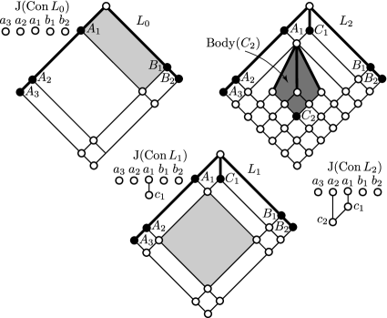
Figure 1. A multifork extension

2.2. Multiforks, lamps and related geometric objects

A 4-cell $X$, that is a cover-preserving 4-element boolean sublattice, is distributive is so is the principal ideal $\mathord{\downarrow}\kern 0.5pt1_{X}:=\{u\in L:u\leq 1_{X}\}$. Given a 4-cell $X$ of $L$ and a positive integer $k$, we can insert a $k$-fold multifork or, if $k$ is unspecified, a multifork into $X$ to obtain a larger slim rectangular lattice, which is called a multifork extension of $L$; see Czédli [1] where this concept is introduced, or see (2.9) and Lemma 2.12 of Czédli [3] where it is recalled, or see only Figure 1 here. In this figure, we add a 1-fold multifork (also called a multifork) to the grey-filled 4-cell of $L_{0}$, and we obtain $L_{1}$. We obtain $L_{2}$ by adding a 3-fold multifork to the grey-filled 4-cell of $L_{1}$.

Next, based on Czédli [3, Definitions 2.3 and 2.6–2.7], we define neon tubes, lamps, and some related geometric concepts. By a neon tube of $L$ we mean an edge $[u,u^{+}]$ such that $u\in\textup{M}(L)$. The boundary neon tubes are of normal slopes while the internal neon tubes are precipitous. For a neon tube ${\mathfrak{n}}=[u,u^{+}]$, we denote $u$ and $u^{+}$ by $\textup{Foot}({\mathfrak{n}})$ and $\textup{Peak}({\mathfrak{n}})$, respectively. Clearly, ${\mathfrak{n}}$ is determined by its foot, $\textup{Foot}({\mathfrak{n}})$. A boundary lamp $I$ is a single boundary neon tube ${\mathfrak{n}}$. (However, we often say that the boundary lamp $I$ has the neon tube ${\mathfrak{n}}$.) If ${\mathfrak{n}}$ is an internal neon tube, then we let

$$\beta_{{\mathfrak{n}}}:=\bigwedge\{\textup{Foot}({\mathfrak{m}}):{\mathfrak{m}} \textup{Peak}({\mathfrak{m}})=\textup{Peak}({\mathfrak{n}})\}$$ is an internal neon tube and (2.4)

and we say that $I:=[\beta_{{\mathfrak{n}}},\textup{Peak}({\mathfrak{n}})]$ is an internal lamp of $L$. The neon tubes ${\mathfrak{m}}$ in (2.4) are the neon tubes of $I$. If $I$ and ${\mathfrak{n}}$ are as above, we use the notations $\textup{Foot}(I)=\beta_{{\mathfrak{n}}}$ and $\textup{Peak}(I)=\textup{Peak}({\mathfrak{n}})$. By a lamp (of $L$) we mean a boundary or internal lamp (of $L$). So lamps are particular intervals and each lamp is determined by its neon tubes. Actually, more is true since we know from Czédli [3, Lemma 3.1] that

each lamp $$I \textup{Foot}(I)$$ is determined by its foot, . (2.5)

This allows us to give the lamps of our diagrams by their feet; these feet are exactly the black-filled elements. See, for example, Figures 1, 2, 3, 4, and 5. We put the name of a lamp close to its black-filled foot.

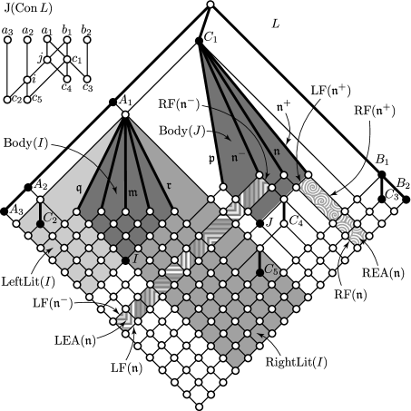
Figure 2. Geometric objects related to lamps

We know from Kelly and Rival [24] that in a planar lattice diagram, each interval determines a geometric region. As in Czédli [3, Definition 2.6], the body of a lamp $I$, denoted by $\textup{Body}(I)$, is the geometric region determined by $I=[\textup{Foot}(I),\textup{Peak}(I)]$. For example, for $L_{2}$ in Figure 1 and its lamp $C_{2}$, $\textup{Body}(C_{2})$ is filled by dark-grey. So are $\textup{Body}(I)$ and $\textup{Body}(J)$ in Figure 3. The region determined by the interval

$$\textup{CircR}(I):=[\bigwedge_{x\prec\textup{Foot}(I)}x,\,\textup{Peak}(I)]$$

is the circumscribed rectangle of $I$; it is a rectangle with all the four sides of normal slopes, and it is always larger than $\textup{Body}(I)$. If $X$ is a neon tube or a lamp, then the left floor of $X$ is the closed line segments of (normal) slope $\pi/4$ between $\textup{Foot}(X)$ and the lower left boundary of the diagram; it is denoted by $\textup{LF}(X)$; see Figure 2 for illustrations. The right floor of $X$, denoted by $\textup{RF}(X)$, is analogously defined. For a lamp $I$ and a neon tube ${\mathfrak{n}}$, their floors are defined by

$$\textup{Floor}(I):=\textup{LF}(I)\cup\textup{RF}(I)\quad\text{ and }\quad\textup{Floor}({\mathfrak{n}}):=\textup{LF}({\mathfrak{n}})\cup\textup{RF}({\mathfrak{n}}).$$ (2.6)

The direct product of two finite non-singleton chains is called a grid. We know from, say, (2.9) and (2.10) of Czédli [3] that for our slim rectangular lattice $L$,

$$\left.\parbox{312.9803pt}{there exists a sequence $L_{0},L_{1},\dots,L_{k}=L$ of slim rectangular lattices and there are distributive 4-cells $H_{i}$ of $L_{i-1}$ such that $L_{0}$ is a grid and, for $1\leq i\leq k$, $L_{i}$ is obtained from $L_{i-1}$ by inserting a multifork into $H_{i}$. Furthermore, the internal lamps of $L$ originate from these multifork extensions and their circumscribed rectangles are $H_{1},\dots,H_{k}$. }\,\,\right\}$$ (2.7)

2.3. What are lamps good for?

For the real answer to this subsection title, see part (ii) of Lemma 2.2 later, which gives a tangible evidence of the importance of lamps.

In our model, each geometric point of a neon tube (as an edge) emits photons but these photon can only go downwards at degree $5\pi/4$ or $7\pi/4$. (That is, to southwest or southeast direction.) For a neon tube ${\mathfrak{n}}$, a geometric point $(x,y)$ of the full geometric rectangle of $L$ is illuminated by ${\mathfrak{n}}$ from the left if the neon tube (as a geometric line segment) has a nonempty intersection with the half-line $\{(x-t,y+t):0\leq t\in\mathbb{R}\}$. The set of geometric points of the full geometric rectangle that are illuminated by ${\mathfrak{n}}$ from the left is denoted by $\textup{RightLit}({\mathfrak{n}})$. (Note “R” in the acronym indicates the points illuminated from the left are on the right.) We define $\textup{LeftLit}({\mathfrak{n}})$ analogously. For a lamp $I$ and a neon tube ${\mathfrak{n}}$, we let

$$\textup{RightLit}(I):=\bigcup\{\textup{RightLit}({\mathfrak{n}}):{\mathfrak{n}}\text{ is a neon tube of }I\},$$ (2.8)

$$\textup{LeftLit}(I):=\bigcup\{\textup{LeftLit}({\mathfrak{n}}):{\mathfrak{n}}\text{ is a neon tube of }I\},$$ (2.9)

$$\textup{Lit}({\mathfrak{n}}):=\textup{LeftLit}({\mathfrak{n}})\cup\textup{RightLit}({\mathfrak{n}}),\text{ and }\textup{Lit}(I):=\textup{LeftLit}(I)\cup\textup{RightLit}(I).$$ (2.10)

In the acronyms above, “Lit” comes from “light”. However, in the text we prefer the verb “illuminate” because of its double meaning: our neon tubes emit physical light and contribute a lot to our comprehension of the congruence lattices of slim semimodular lattices.

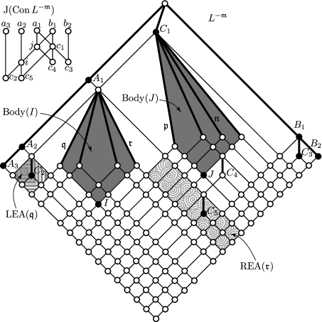
Figure 3. $L^{\mathfrak{m}}$, obtained from Figure 2 according to (2.16)

While the geometric sets defined in (2.8)–(2.10) here were sufficient for the proofs in Czédli [3], the present paper has to introduce some smaller sets as follows. Let ${\mathfrak{n}}$ be a neon tube. The unique lamp to which ${\mathfrak{n}}$ belongs will be denoted by $I=I_{\mathfrak{n}}$. Below, we assume that $I$ is not a boundary lamp.

$$\left.\parbox{278.83708pt}{If ${\mathfrak{n}}$ is the leftmost neon tube of $I$, then $\textup{LEA}({\mathfrak{n}}):=\textup{LeftLit}({\mathfrak{n}})\setminus\textup{CircR}(I)$. Otherwise, let ${\mathfrak{n}}^{-}$ denote the left neighbour of ${\mathfrak{n}}$ among the neon tubes of $I$, and let $\textup{LEA}({\mathfrak{n}})$ be the (closed convex) geometric rectangle with sides $\textup{LF}({\mathfrak{n}})$, $\textup{LF}({\mathfrak{n}}^{-})$, a part of $\textup{RF}({\mathfrak{n}}^{-})$, and a part of the lower boundary of $L$. We define $\textup{REA}({\mathfrak{n}})$, the left-right symmetric counterpart of $\textup{LEA}({\mathfrak{n}})$, analogously.}\,\,\right\}$$ (2.11)

The choice of the acronyms above will be explained a bit later.

For example, $\textup{LEA}({\mathfrak{n}})$ and $\textup{REA}({\mathfrak{n}})$ in Figure 2 are the zigzag-filled rectangle and the spiral-filled rectangle, respectively. In Figure 3, ${\mathfrak{q}}$ is the leftmost neon tube of $I$ and $\textup{LEA}({\mathfrak{q}})$ is the zigzag-filled rectangle while $\textup{REA}({\mathfrak{r}})$ for the rightmost neon tube ${\mathfrak{r}}$ is the spiral-filled rectangle. If ${\mathfrak{n}}$ is a boundary lamp, then exactly one of $\textup{LEA}({\mathfrak{n}})$ and $\textup{REA}({\mathfrak{n}})$ is of positive geometric area while the other is a line segment or $\emptyset$.

For a subset $Y$ of the plane, let $\textup{GInt}(Y)$ denote the topological (in other words, geometric) interior of $Y$. Observe that

$$\left.\parbox{210.55022pt}{for distinct neon tubes ${\mathfrak{n}}$ and ${\mathfrak{n}}^{\prime}$ of a lamp, $\textup{GInt}(\textup{LEA}({\mathfrak{n}}))\cap\textup{GInt}(\textup{LEA}({\mathfrak{n}}^{\prime}))=\emptyset$ and, analogously, $\textup{GInt}(\textup{REA}({\mathfrak{n}}))\cap\textup{GInt}(\textup{REA}({\mathfrak{n}}^{\prime}))=\emptyset$}\,\,\right\}$$ (2.12)

This motivates us to call $\textup{LEA}({\mathfrak{n}})$ and $\textup{REA}({\mathfrak{n}})$ the left exclusive area and the right exclusive area of ${\mathfrak{n}}$; this is where the acronyms in (2.11) come from. Later, by an exclusive area of ${\mathfrak{n}}$ we mean one of $\textup{LEA}({\mathfrak{n}})$ and $\textup{REA}({\mathfrak{n}})$. By a trivial induction based on (2.7) or using trajectories introduced in Czédli and Schmidt [12], we obtain easily that

for any 4-cell $$C {\mathfrak{n}} {\mathfrak{m}} \textup{LEA}({\mathfrak{n}})\cap\textup{REA}({\mathfrak{m}}) C$$, there are unique neon tubes and such that is the geometric rectangle determined by . (2.13)

2.4. On the number of neon tubes

In the whole paper,

$$\left.\parbox{213.39566pt}{$\textup{Lamp}(L)$ and $\textup{NTube}(L)$ denote the set of lamps and that of neon tubes of $L$, respectively.}\,\,\right\}$$ (2.14)

On the set $\textup{Lamp}(L)$ of lamps of $L$, we define five relations; the first four are taken from Czédli [3, Definition 2.9] while the last two are new. Note that using the remaining two out of the six relations of [3, Definition 2.9] together with trivial inclusions like $\textup{GInt}(X)\subseteq X$ or, for a neon tube ${\mathfrak{n}}$ of a lamp $I$, $\textup{LEA}({\mathfrak{n}})\subseteq\textup{LeftLit}(I)$, one could easily define even more relations (but this does not seem to be useful).

Definition 2.1 (Relations defined for lamps).

Let $L$ be a slim rectangular lattice with a fixed $\mathcal{C}_{1}$-diagram. For $I,J\in\textup{Lamp}(L)$,

1. let $(I,J)\in{{\rho}}_{\textup{alg}}$ mean that $\textup{Peak}(I)\leq\textup{Peak}(J)$, $I$ is an internal lamp, and $\textup{Foot}(I)\not\leq\textup{Foot}(J)$;

2. let $(I,J)\in{{\rho}}_{\textup{foot}}$ mean that $I\neq J$, $\textup{Foot}(I)\in\textup{Lit}(J)$, and $I$ is an internal lamp;

3. let $(I,J)\in{{\rho}}_{\textup{infoot}}$ mean that $I\neq J$, $\textup{Foot}(I)\in\textup{GInt}(\textup{Lit}(J))$, and $I$ is an internal lamp;

4. let $(I,J)\in{{\rho}}_{\textup{Body}}$ mean that $I\neq J$, $\textup{Body}(I)\subseteq\textup{Lit}(J)$, and $I$ is an internal lamp;

5. let $(I,J)\in{{\nu}}_{\textup{infoot}}$ mean that $I$ is an internal lamp, $I\neq J$ and $J$ has a neon tube ${\mathfrak{n}}$ such that $\textup{Foot}(I)\in\textup{GInt}(\textup{LEA}({\mathfrak{n}}))$ or $\textup{Foot}(I)\in\textup{GInt}(\textup{REA}({\mathfrak{n}}))$; and, finally,

6. let $(I,J)\in{{\nu}}_{\textup{LRCircR}}$ mean that $I$ is an internal lamp, $I\neq J$ and $J$ has a neon tube ${\mathfrak{n}}$ such that $\textup{CircR}(I)\subseteq\textup{LEA}({\mathfrak{n}})$ or $\textup{CircR}(I)\subseteq\textup{REA}({\mathfrak{n}})$.

Now we are in the position to formulate the key lemma for this section. For $x,y\in L$, the least congruence containing $(x,y)$ is denoted by $\textup{con}(x,y)$.

Lemma 2.2 (Neon Tube Lemma).

Let $L$ be a slim rectangular lattice with a fixed $\mathcal{C}_{1}$-diagram; then the following three assertions hold.

1. The six relations described in Definition 2.1 are all equal. Furthermore, they are equal to the relations given in Czédli [3, Definition 2.9].

2. Let $\leq$ denote the reflexive transitive closure of ${{\rho}}_{\textup{alg}}$. Then $\leq$ is a partial order and the poset $(\textup{Lamp}(L);\leq)$ is isomorphic to the poset $(\textup{J}(\operatorname{Con}L);\leq)$ of nonzero join-irreducible congruences of $L$ with respect to the ordering inherited from $\operatorname{Con}L$. In fact, the map $\varphi\colon\textup{Lamp}(L)\to\textup{J}(\operatorname{Con}L)$, defined by $[p,q]\mapsto\textup{con}((p,q))$, is an order isomorphism.

3. If $I\prec J$ (that is, $I$ is covered by $J$) in $\textup{Lamp}(L)$, then $(I,J)\in{{\rho}}_{\textup{alg}}$.

Before the proof, several comments are reasonable. While ${{\rho}}_{\textup{foot}}$ is the mildest geometric condition on $(I,J)$, ${{\nu}}_{\textup{LRCircR}}$ is (seemingly) more restrictive that any other relation described in [3, Definition 2.9]. This is why the Neon Tube Lemma is a stronger than its counterpart, Lemma 2.11 of Czédli [3].

In addition to lamps (and neon tubes), there are other approaches to the congruence lattices of slim rectangular lattices: the Swing Lemma from Grätzer [18] (see also Czédli, Grätzer and Lakser [8] and Czédli and Makay [10] for secondary approaches), the Trajectory Coloring Theorem from Czédli [1], and even Lemma 2.36 (about the join dependency relation of Day [15], for any finite lattice) in Freese, Ježek and Nation [16]. Even though the differences among the four different approaches are not so big and most of these approaches would probably be appropriate to prove the results of this paper on congruence lattices of slim semimodular lattices, we believe that our approach based on lamps (and neon tubes) gives the best insight into the congruence lattices of slim rectangular (and, therefore, those of slim semimodular) lattices. In addition to the present paper, this is witnessed by Czédli [3] and Czédli and Grätzer [7]. Indeed, with two early exceptions, all the known of these congruence lattices have been found and first proved (or, at least, first proved) by lamps (and neon tubes).

Proof of Lemma 2.2.

Recall that Czédli [3, Definition 2.9] defines a relation ${{\rho}}_{\textup{CircR}}$ on $\textup{Lamp}(L)$ as follows: a $(I,J)\in{{\rho}}_{\textup{CircR}}$ if $I$ is an internal lamp, $\textup{CircR}(I)\subseteq\textup{Lit}(J)$, and $I\neq J$.

It suffices to prove the first sentence of part (i) since the rest of the lemma follows from its counterpart, [3, Lemma 2.11], which also contains ${{\rho}}_{\textup{alg}}$, ${{\rho}}_{\textup{foot}}$, ${{\rho}}_{\textup{infoot}}$, and ${{\rho}}_{\textup{Body}}$. Fortunately, the proof of [3, Lemma 2.11] also proves the above-mentioned first sentence provided we observe the following.

We know from [3, Lemma 2.11] that ${{\rho}}_{\textup{alg}}={{\rho}}_{\textup{foot}}={{\rho}}_{\textup{CircR}}$. Assume that $(I,J)\in{{\rho}}_{\textup{CircR}}$. Using (2.7), which is the combination of (2.9) and (2.10) of [3], $J$ comes sooner than $I$. When $J$ has just arrived, the exclusive areas of its neon tubes are separated by edges. By (2.11) of [3], these sets are still separated by edges when $I$ arrives. By planarity, these edges cannot cross $\textup{CircR}(I)$. Hence the covering square into which $I$ enters (and which is geometrically $\textup{CircR}(I)$) is a subset of an exclusive area of a neon tube of $J$.

Keeping the above paragraph in mind, the (long) proof of [3, Lemma 2.11] works in the present situation. This completes the proof of the Neon Tube Lemma. ∎

Before formulating an easy consequence (under the name “lemma”) of the Three Neon Tubes Lemma, we define two easy-to-understand concepts. A neon tube ${\mathfrak{n}}$ of $L$ is secondary if there is no $I\in\textup{Lamp}(L)$ such that $\textup{Foot}(I)\in\textup{GInt}(\textup{LEA}({\mathfrak{n}}))\cup\textup{GInt}(\textup{REA}({\mathfrak{n}}))$. Equivalently, if for every $I\in\textup{Lamp}(L)$, neither $\textup{CircR}(I)\subseteq\textup{LEA}({\mathfrak{n}})$ nor $\textup{CircR}(I)\subseteq\textup{REA}({\mathfrak{n}})$. In the opposite case when there is an $I\in\textup{Lamp}(L)$ such that $\textup{Foot}(I)\in\textup{GInt}(\textup{LEA}({\mathfrak{n}}))\cup\textup{GInt}(\textup{REA}({\mathfrak{n}}))$, we say that ${\mathfrak{n}}$ is a primary neon tube. For example, $\{A_{1},A_{2},A_{3},B_{1},B_{2},C_{1},{\mathfrak{p}},{\mathfrak{q}},{\mathfrak{r}}\}$ is the set of primary neon tubes in Figure 2. (Some but not all of the primary neon tubes are lamps.) The rest of the neon tubes, including ${\mathfrak{m}}$, ${\mathfrak{n}}^{-}$, ${\mathfrak{n}}$, and ${\mathfrak{n}}^{+}$, are secondary.

The following concept is self-explanatory: we say that ${\mathfrak{n}}_{1},{\mathfrak{n}}_{2},{\mathfrak{n}}_{3}$ are three geometrically consecutive neon tubes if they belong to the same lamp $I$ and, among the feet of all neon tubes of $I$, $\textup{Foot}({\mathfrak{n}}_{i})$ is immediately to the right of $\textup{Foot}({\mathfrak{n}}_{i-1})$ for $i\in\{2,3\}$. For example, ${\mathfrak{n}}^{-}$, ${\mathfrak{n}}$, and ${\mathfrak{n}}^{+}$ are three geometrically consecutive neon tubes in Figure 2 but ${\mathfrak{q}}$, ${\mathfrak{m}}$, and ${\mathfrak{r}}$ are not.

Lemma 2.3 (Three Neon Tubes Lemma).

Let ${\mathfrak{n}}_{1}$, ${\mathfrak{m}}={\mathfrak{n}}_{2}$, and ${\mathfrak{n}}_{3}$ be three consecutive neon tubes of our slim rectangular lattice $L$ such that each of these three neon tubes is secondary. Then $L^{-{\mathfrak{m}}}$, to be defined in (2.16), is also a slim rectangular lattice, $\operatorname{Con}{L^{-{\mathfrak{m}}}}\cong\operatorname{Con}L$, and $|\textup{NTube}(L^{-{\mathfrak{m}}})|=|\textup{NTube}(L)|-1$.

Proof.

Clearly, ${\mathfrak{m}}$ is an internal neon tube. Keeping (2.2) in mind, the left and right boundary chains of $L$ are denoted by $\textup{C}_{\textup{left}}(L)$ and $\textup{C}_{\textup{right}}(L)$, respectively. For $a\in L$, the ideal $\{x\in L:x\leq a\}$ will be denoted by $\mathord{\downarrow}\kern 0.5pta$. Let $\textup{ljc}(a)$ and $\textup{rjc}(a)$ stand for the largest element of $\textup{C}_{\textup{left}}(L)\cap\mathord{\downarrow}\kern 0.5pta$ and $\textup{C}_{\textup{right}}(L)\cap\mathord{\downarrow}\kern 0.5pta$, respectively. (These acronyms come from left join coordinate and right join coordinate, respectively; note that both $\textup{ljc}(a)$ and $\textup{rjc}(a)$ belong to $\textup{J}(L)\cup\{0\}$.) Let

$$F({\mathfrak{m}}) :=[\textup{ljc}(\textup{Foot}({\mathfrak{m}})),\textup{Foot}({\mathfrak{m}})]\cup[\textup{rjc}(\textup{Foot}({\mathfrak{m}})),\textup{Foot}({\mathfrak{m}})]\cup\{\textup{Peak}({\mathfrak{m}})\},$$ (2.15)

$$L^{\prime} :=L^{-{\mathfrak{m}}}:=L\setminus F({\mathfrak{m}}).$$ (2.16)

Note that $F({\mathfrak{m}})$ is a so-called fork with top edge ${\mathfrak{m}}$; this concept was introduced in Czédli and Schmidt [13]. We know from [13, Lemma 20] and from the fact that the corners are clearly outside $F({\mathfrak{m}})$ that $L^{-{\mathfrak{m}}}$ is a slim rectangular lattice. For the intervals occurring in (2.15), we know from [13, Lemma 18] that,

$$[\textup{ljc}(\textup{Foot}({\mathfrak{m}})),\textup{Foot}({\mathfrak{m}})] [\textup{rjc}(\textup{Foot}({\mathfrak{m}})),\textup{Foot}({\mathfrak{m}})]$$ and are chains. (2.17)

Furthermore, as it is implicit in, say, Czédli and Schmidt [13], we can assume that the $\mathcal{C}_{1}$-diagram of $L^{-{\mathfrak{m}}}$ is obtained from that of $L$ in the natural way: we omit the elements of $F({\mathfrak{m}})$ from the diagram; see how Figure 3 is obtained from Figure 2.

We know from, say, Theorem 2.1 and Corollary 2.2 of Czédli, Ozsvárt and Udvari [11] that for any SPS lattice $K$, $\textup{length}(K)=|\textup{M}(K)|$. When passing from $L$ to $L^{-{\mathfrak{m}}}$, $\textup{ljc}(\textup{Foot}({\mathfrak{m}}))$ is the only element that we remove from the left boundary chain of $L$. Since the left boundary chain is a maximal chain and any two finite maximal chains of a semimodular lattice are of the same length, we obtain that $\textup{length}(L^{-{\mathfrak{m}}})=\textup{length}(L)-1$. Hence, $|\textup{NTube}(L^{-{\mathfrak{m}}})|=|\textup{M}(L^{-{\mathfrak{m}}})|=\textup{length}(L^{-{\mathfrak{m}}})=\textup{length}(L)-1=|\textup{M}(L)|-1=|\textup{NTube}(L)|-1$, as required.

Let $L_{0}$, $L_{1}$, …, $L_{k}=L$ be a sequence according to (2.7). For $i=1,\dots,k$, let $Q_{i}$ be the lamp that comes to existence when we pass from $L_{i-i}$ to $L_{i}$; so $Q_{i}$ is in $\textup{Lamp}(L_{i})$ and $\textup{Lamp}(L)$ but it is not in $\textup{Lamp}(L_{i-1})$. We know that $\textup{CircR}(Q_{i})=H_{i}$ and $\textup{Lamp}(L)=\{Q_{1},\dots,Q_{k}\}$. Assume that ${\mathfrak{m}}$ belongs to $Q_{j}$. The (2.7) sequence for $L^{\prime}:=L^{-{\mathfrak{m}}}$ will be denoted by $L^{\prime}_{0}$, $L^{\prime}_{1}$, …, $L^{\prime}_{k}=L^{\prime}$. We choose this sequence so $L^{\prime}_{i}=L_{i}$ for $i<j$, and their diagrams are also the same. Note that $j>1$ since $Q_{j}$ is not a boundary lamp.

Let ${\mathfrak{n}}$ be a primary neon tube of $Q_{j}$, and let ${\mathfrak{n}}^{-}$ and ${\mathfrak{n}}^{+}$ be its left neighbour and right neighbour, respectively. (The case when ${\mathfrak{n}}^{-}$ or ${\mathfrak{n}}^{+}$ does not exists is simpler and will not be detailed.) Since ${\mathfrak{m}}$ is secondary and it is sitting between two secondary neon tubes, none of ${\mathfrak{n}}$, ${\mathfrak{n}}^{-}$, and ${\mathfrak{n}}^{+}$ is ${\mathfrak{m}}$, whereby none of them is removed. Hence, none of $\textup{LF}({\mathfrak{n}}^{-})$, $\textup{RF}({\mathfrak{n}}^{-})$, $\textup{LF}({\mathfrak{n}})$, $\textup{RF}({\mathfrak{n}})$, $\textup{LF}({\mathfrak{n}}^{+})$, and $\textup{RF}({\mathfrak{n}}^{+})$ changes when we remove ${\mathfrak{m}}$. These six lines together with the lower boundary of $L$ form $\textup{LEA}({\mathfrak{n}})$ and $\textup{REA}({\mathfrak{n}})$. Hence

$$\left.\parbox{227.62204pt}{$\textup{LEA}({\mathfrak{n}})$ and $\textup{REA}({\mathfrak{n}})$ remain the same for any primary neon tube ${\mathfrak{n}}$ of $L_{j}$ when ${\mathfrak{m}}$ is removed.}\,\,\right\}$$ (2.18)

Furthermore, since $\textup{Body}(Q_{j})$ only depends on its leftmost neon tube and rightmost neon tube, it does not depend on ${\mathfrak{m}}$, and so

the removal of $${\mathfrak{m}} \textup{Body}(Q_{j})$$ does not change . (2.19)

We are going to use $\mathrel{\overset{\textup{geo}}{=}}$ to indicate that two geometrical objects (or two sets of such objects) are exactly the same in a fixed coordinate system of the Euclidean plane $\mathbb{R}^{2}$. We know that $L_{j-1}$ and $L^{\prime}_{j-1}$ are the same as well as their diagrams. This fact and (2.19) gives that

$$\{\textup{Body}(I):I\in\textup{Lamp}(L^{\prime}_{j})\}\mathrel{\overset{\textup{geo}}{=}}\{\textup{Body}(I):I\in\textup{Lamp}(L_{j})\}$$ (2.20)

Furthermore, it follows from (2.18) that

$$\begin{aligned} \{\textup{LEA}({\mathfrak{n}})&:{\mathfrak{n}}\in\textup{Lamp}(L^{\prime}_{j})\text{ and }{\mathfrak{n}}\text{ is primary }\}\cr&\mathrel{\overset{\textup{geo}}{=}}\{\textup{LEA}({\mathfrak{n}}):{\mathfrak{n}}\in\textup{Lamp}(L_{j})\text{ and }{\mathfrak{n}}\text{ is primary }\}\text{ and}\end{aligned}$$ (2.21)

$$\begin{aligned} \{\textup{REA}({\mathfrak{n}})&:{\mathfrak{n}}\in\textup{Lamp}(L^{\prime}_{j}),\text{ and }{\mathfrak{n}}\text{ is primary}\}\cr&\mathrel{\overset{\textup{geo}}{=}}\{\textup{REA}({\mathfrak{n}}):{\mathfrak{n}}\in\textup{Lamp}(L_{j})\text{, and }{\mathfrak{n}}\text{ is primary}\}\text{ and }\cr\end{aligned}$$ (2.22)

$$L^{\prime}_{j} L_{j}$$ is a sublattice (and subdiagram) of . (2.23)

Trajectories were introduced in Czédli and Schmidt [12]; it is convenient to look into Czédli [3, Definition 2.13] for their definition. We know from the sentence following (2.23) in [3] that the neon tubes of $L$ are exactly the top edges of the trajectories of $L$. We claim that

$$\left.\parbox{227.62204pt}{if \eqref{eq:vnwzlFzsghTflda}, \eqref{eq:vnwzlFzsghTfldb}, \eqref{eq:vnwzlFzsghTfldc}, and \eqref{eq:vnwzlFzsghTfldd} hold for some $i$ (in place of $j$) and $i<k$, then they also hold for $i+1$.}\,\,\right\}$$ (2.24)

This is almost trivial (at least, visually). Assume that (2.20)–(2.23) hold for some $i$ (in place of $j$) and $i<k$. To obtain $L_{i+1}$ from $L_{i}$, we pick a distributive 4-cell $H_{i+1}$ of $L_{i}$. As a geometric area, $H_{i+1}$ is of the form $\textup{LeftLit}({\mathfrak{n}}^{\flat})\cap\textup{RightLit}({\mathfrak{n}}^{\sharp})$, where ${\mathfrak{n}}^{\flat}$ is the top edge of the trajectory containing the upper right edge of $H_{i+1}$ while ${\mathfrak{n}}^{\sharp}$ is the top edge of the trajectory containing the upper left edge of $H_{i+1}$. Thus, using the validity of (2.21) and (2.22) of $i$, it follows that $H_{i+1}$ is geometrically the same for $L^{\prime}_{i}$ as for $L_{i}$. Hence, geometrically exactly the same multifork can be (and is) inserted into $H_{i+1}$ in case of $L^{\prime}_{i}$ as in case of $L_{i}$. In fact, $\textup{CircR}(Q_{j+1})=\textup{LeftLit}({\mathfrak{n}}^{\flat})\cap\textup{RightLit}({\mathfrak{n}}^{\sharp})$, both in $L^{\prime}_{j+1}$ and in $L_{j+1}$. Thus, we conclude (2.24).

Since $L^{\prime}=L^{\prime}_{k}$ and $L=L_{k}$, it follows from (2.24) that (2.20) holds for $L^{\prime}$ and $L$ (in place of $L^{\prime}_{j}$ and $L_{j}$, respectively). Now it is clear that ${{\rho}}_{\textup{foot}}$ is the same for $L^{\prime}$ as it is for $L$. Hence, we conclude from Lemma 2.2 that $\bigl{(}\textup{J}(\operatorname{Con}{L^{\prime}}),\leq\bigr{)}\cong\bigl{(}\textup{J}(\operatorname{Con}{L}),\leq\bigr{)}$. By the well-known structure theorem of finite distributive lattices, see, for example, Grätzer [17, Theorem 107], $L^{\prime}\cong L$, as required. This completes the proof of Lemma 2.3. ∎

Next, we prove the following easy lemma. The height of an element $x$ of a finite semimodular lattice will be denoted by $0pt(x)$; it is the length of the ideal $\mathord{\downarrow}\kern 0.5ptx$.

Lemma 2.4.

Let $H$ be distributive $4$-cell of a slim rectangular lattice $L$, and let $L^{\prime}$ be the (necessarily slim rectangular) lattice that we obtain from $L$ by inserting a $k$-fold multifork into $H$. Then $|L^{\prime}|=|L|+k\cdot 0pt({1_{H}})+k(k+1)/2$ and $\textup{length}(L^{\prime})=\textup{length}(L)+k$.

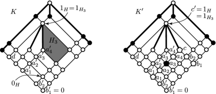
Figure 4. Illustrating the proof of Lemma 2.4

Proof.

Since $L$ and $L^{\prime}$ are semimodular, their lengths are witnessed by their left boundary chains. Hence, the equality $\textup{length}(L^{\prime})=\textup{length}(L)+k$ is clear from the definition of adding multiforks.

The structure theorem based on multiforks, see (2.7), is more advantageous than that based on forks, in Czédli and Schmidt [13, Lemma 22], since while multiforks are only added to distributive 4-cells but this is not so in case if we are only allowed to add forks. However, in this proof, it is better to add $k$ forks, on by one, instead of adding a $k$-fold multifork. So we insert, one by one, $k$ forks (that is, $1$-fold multiforks $k$ times) into appropriate 4-cells $H_{1}:=H$, $H_{2}$, …, $H_{k}$ with the same top $1_{H}$. Since

$$(1+0pt(1_{H}))+(2+0pt(1_{H}))+\dots+(k+0pt(1_{H}))$$

with $k$ (outer) summands is $k\cdot 0pt({1_{H}})+k(k+1)/2$, it suffices to show that for $i=1,\dots,k$, if $K$ and $K^{\prime}$ denote the lattice right before and right after inserting the $i$-th multifork into $H_{i}$, then

$$\left.\parbox{173.56198pt}{$0pt_{K^{\prime}}(1_{H_{i}})=0pt_{K}(1_{H_{i}})+1$ and $|K^{\prime}|=|K|+0pt_{K^{\prime}}(1_{H_{i}})$.}\,\,\right\}$$ (2.25)

Instead of a formal and lengthy consideration, we use Figure 4 to verify (2.25). This figure, where $i=3$, shows how we insert the $i$-th fork into the grey-filled 4-cell $H_{3}$ of $K$ to obtain $K^{\prime}$. Implicitly, we will use that $1_{H_{i}}=1_{H}$ and $\mathord{\downarrow}\kern 0.5pt1_{H}$ was distributive before any fork was inserted into $H$. With $t=4$ and $s=2$, the new elements are $a_{1},\dots,a_{t}$, $b_{1},\dots,b_{s}$, and $c$; these elements are pentagon-shaped. Assigning an old element $x^{\prime}$ to each new element $x$, we get a maximal chain

$$0=b_{1}^{\prime}\prec\dots\prec b_{s}^{\prime}\prec a_{1}^{\prime}\prec\dots\prec a_{t}^{\prime}\prec c^{\prime}=0pt_{K}(1_{H_{i}})$$

in $\mathord{\downarrow}\kern 0.5pt_{K}(1_{H_{i}})$. Hence, the number of new elements is $0pt_{K}(1_{H_{i}})+1$. On the other hand, with $d:=\textup{ljc}(1_{H_{i}})$, both $\mathord{\downarrow}\kern 0.5pt_{\kern-2.0ptK}d$ and $[d,1_{H_{i}}]$ are chains by Grätzer and Knapp [23, Lemma 4]. Hence, $C:=\mathord{\downarrow}\kern 0.5pt_{\kern-2.0ptK}d\cup[d,1_{H_{i}}]$ is a maximal chain in $\mathord{\downarrow}\kern 0.5pt_{\kern-2.0ptK}1_{H_{i}}$. Since exactly one element, $a_{1}$, is added to this chain when we pass from $K$ to $K^{\prime}$, we obtain that $0pt_{K^{\prime}}(_{H_{i}})=0pt_{K}(_{H_{i}})+1$. Now that we have the first half of (2.25), the number of new elements is $0pt_{K}(1_{H_{i}})+1=0pt_{K^{\prime}}(1_{H_{i}})$. We have verified (2.25), and the proof of Lemma 2.4 is complete. ∎

The following observation only gives a very rough upper bound on the size $|L|$ of $L$ but even such a bound will be sufficient to derive a corollary.

Observation 2.5.

Let $D$ be a finite distributive lattice such that $D$ is representable, that is, $D$ is isomorphic to the congruence lattice of a slim rectangular lattice. Then, with the notation $n:=|\textup{J}(D)|$, there exists a slim rectangular lattice $L$ such that $\operatorname{Con}L\cong D$, $\textup{length}(L)\leq 3n^{2}$, and $|L|\leq 9n^{4}$.

Proof.

Assume that $L$ is a slim rectangular lattice of minimal size $|L|$ such that $\operatorname{Con}L\cong D$. We know from (ii) of Lemma 2.2 here, that is, from Czédli [3] that $(\textup{Lamp}(L);\leq)\cong(\textup{J}(D);\leq)$. Hence $|\textup{Lamp}(L)|=n$. There are at least two boundary lamps (since $L$ is rectangular), so there are at most $n-2$ internal lamps. Observe that if a neon tube ${\mathfrak{n}}$ of a lamp $J$ is primary, then $(I,J)\in{{\nu}}_{\textup{infoot}}$ for some (necessarily internal) lamp $I$. By Lemma 2.3, and the minimality of $|L|$, $J$ cannot have three consecutive secondary neon tubes. Thus,

$$J 3(n-2)+2=3n-4$$ has at most neon tubes. (2.26)

So, taking into account that a boundary lamp has only a single neon tubes, the total number of neon tubes is at most $n+(n-2)\cdot(3n-4)=3n^{2}-9n+8$. Each new lamp with $i$ neon tubes comes to existence by adding an $i$-fold multifork, which increases the length by $i$; see lemma 2.4. This fact, $|\textup{NTube}(L)|\leq 3n^{2}-9n+8$, and the obvious $\textup{length}(L_{0})\leq n$ yield that $\textup{length}(L)\leq n+3n^{2}-9n+8\leq 3n^{2}$, as required.

Finally, to obtain the last inequality stated in the observation, it suffices two show that a slim rectangular lattice (in fact, any SPS lattice) $L$ of length $\ell$ has at most $\ell^{2}$ elements. We can argue for this easily as follows. By slimness (in the sense of Czédli and Schmidt [12]), $\textup{J}(L)$ is the union of two chains, $C_{1}$ and $C_{2}$. By rectangularity and the definition of $\textup{J}(L)$, none of $0$ and $1$ is in $C_{1}$ and $C_{2}$. So, $|C_{1}|\leq\ell-1$ and $|C_{2}|\leq\ell-1$. Since each element of $L\setminus\{0\}$ is of the form $c_{1}\vee c_{2}$ with $c_{1}\in C_{1}$ and $c_{2}\in C_{2}$, $L$ has at most $1+(\ell-1)^{2}\leq\ell^{2}$ elements, indeed. This completes the proof of the observation. ∎

Recall that slim semimodular lattices are also called SPS lattices.

Corollary 2.6.

There is an algorithm to decide whether a given finite distributive lattice $D$ is isomorphic to the congruence lattice of some SPS lattice $L$; if the answer is affirmative, then the algorithm yields a slim rectangular lattice $L$ such that $D\cong\operatorname{Con}L$.

Proof.

Let $n:=|\textup{J}(D)|$. By (2.3), it suffices to deal with the question whether there is a slim rectangular lattice $L$ of minimal size such that $\operatorname{Con}L\cong D$. By Observation 2.5, if such an $L$ exists, then $|L|\leq 9n^{4}$. Since we can clearly list all the at most $9n^{4}$-element lattices, we can check which one of them are slim rectangular lattices, and for each such lattice $L$ we can decide whether $\operatorname{Con}L\cong D$, we conclude the corollary. ∎

3. Notes on the algorithm

The algorithm described in the proof of Corollary 2.6 is far from being effective. Even if we do not know if there is a good (better than exponential) algorithm to decide whether there is an SPS lattice with $\operatorname{Con}L\cong\operatorname{Con}D$, we collect some facts about the weakness of the algorithm described in the proof above; these comments offer some improvements.

Remark 3.1.

Instead of constructing all lattices with at most $9n^{4}$-elements, it is faster (but not fast enough) to list all slim rectangular lattices of length at most $3n^{2}$; this $3n^{2}$ comes from Observation 2.5. But even if we do so, we are still far from a good algorithm. Indeed, we know from Czédli, Dékány, Gyenizse, and Kulin [6] that the number of slim rectangular lattices of length $k$ is asymptotically $(k-2)!\cdot e^{2}/2$, where $e$ is the famous mathematical constant $\lim_{n\to\infty}(1+1/n)^{n}\approx 2.718\,281\,828$. Thus, there are about

$$x(n):=(e^{2}/2)\cdot\sum_{k=2}^{3n^{2}}(k-2)!$$ (3.1)

many slim rectangular lattices to verify, and we could hardly verify that many. Indeed, say,

$$x(5)\approx 0.167\cdot 10^{107}\text{ and }x(9)\approx 0.3637\cdot 10^{472},$$ (3.2)

indicate that even with the help of a computer, the method given so far is not enough to decide whether $D$ with $|\textup{J}(D)|$ can be represented in the required way.

Remark 3.2.

Since our purpose was to give short proofs, the estimates $3n^{2}$ and $9n^{4}$ in Observation 2.5 are far from being optimal, because of several reasons. First, our computation was based on the Three Neon Tubes Lemma, that is, Lemma 2.3, although the “Two Neon Tubes Lemma” (asserting that if there are two consecutive secondary neon tubes, then one of them can be removed) seems also be true. (The “Two Neon Tubes Lemma” would require a more complicated and much longer proof than Lemma 2.3 while not leading to a feasible algorithm, so we neither prove nor use this lemma.) Second, (2.26) is a rather weak estimate for most $J\in\textup{Lamp}(L)$; indeed, if $I\in\textup{Lamp}(L)$ witnesses that a neon tube ${\mathfrak{n}}$ of $J$ is primary, that is, if $\textup{Foot}(I)$ belongs to $\textup{GInt}(\textup{LEA}({\mathfrak{n}}))\cup\textup{GInt}(\textup{REA}({\mathfrak{n}}))$, then $I<J$. So if $\mathord{\downarrow}\kern 0.5ptJ$, understood in $(\textup{Lamp}(L),\leq)$, is a small set, then only few neon tubes of $J$ can be primary, and Lemma 2.3 yields that $J$ only has few neon tubes. Furthermore, we know from Lemma 2.2 that each lower cover of $J$ is illuminated by a primary neon tube of $J$, but the rest of lamps belonging to $\mathord{\downarrow}\kern 0.5ptJ$ need not be.

Remark 3.3.

Even if we used the ideas above to improved the algorithm given Corollary 2.6, it would not be feasible enough. One of the reasons is that if we construct all slim rectangular lattices of a given length $k$ without keeping the poset $\textup{J}(L)$ in mind, then approximately $x(k)$ many lattices, so too many lattices should be constructed; see (3.1).

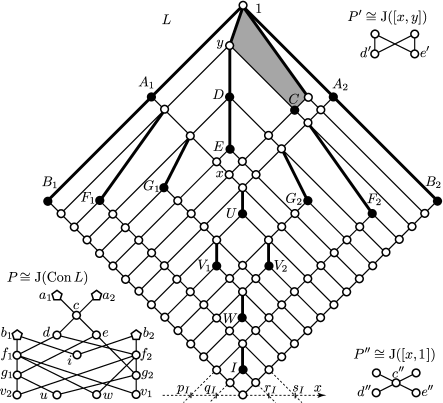
Figure 5. The secondary neon tube of $C$ cannot be omitted

Remark 3.4.

A secondary neon tube can quite frequently be omitted but not always. We present some examples. In the first example, let $Y$ denote the four-element “Y-shaped” poset $\{0,c,a,b\}$ such that $0\prec c$, $c\prec a$, and $c\prec b$ is a full list of coverings. Then $c$ only has one lower cover, there exists a slim rectangular lattice $L$ such that $\textup{J}(\operatorname{Con}L)\cong Y$, but for every such $L$, the lamp $C\in\textup{Lamp}(L)$ corresponding to $c\in Y$ necessarily has at least one secondary neon tube.

The second example, given by Figure 5, shows how to represent the poset $P$ on the bottom left as $\textup{J}(\operatorname{Con}L)$ where $L$ is the slim rectangular lattices drawn in the middle. As usually in the paper, $x\in P$ is represented by $X\in\textup{Lamp}(L)$, for any letter $x$. Note that $\textup{Body}(C)$ is grey-filled in the figure. Observe that $c$ has two lower covers (so more than $c$ in the first example) but $C$ still has only two neon tube. Furthermore, the neon tube of $C$ on the left is secondary.

Figure 5 also shows how the represent $P^{\prime}$ and $P^{\prime\prime}$, drawn on the right, by certain intervals of $L$; these intervals are slim rectangular lattices. It would be easy to construct similar examples with arbitrary many minimal elements while keeping the subposet of $P^{\prime}$ or $P^{\prime\prime}$ formed by the non-minimal elements unchanged.

As another example, we mention that $f_{1}$ in Figure 5 has three lower covers but $F_{1}\in\textup{Lamp}(L)$ only has one neon tube.

Remark 3.4 is our excuse that we do not try to determine the minimal number of neon tubes of a lamp $X$ representing an element $x$ of a poset.

4. An algorithm based on illuminated sets

In this section, we are going to point out that it is frequently advantageous to base our investigation on $\textup{LitSet}(L)$ rather than $\textup{Lamp}(L)$; in this way we can reduce many problems about $\operatorname{Con}L$ to combinatorial geometric problems about illuminated sets. Furthermore, Lemma 4.3 of this section, which is formulated both for lamps and for illuminated sets, will be used in subsequent sections.

The paragraph we commence here is to warn the reader. The algorithm described in this section is much more complicated than the one described by (the proof of) Corollary 2.6. Indeed, while one can understand in a second that checking all lattices $L$ with at most $9\cdot|\textup{J}(D)|^{4}$ elements is an algorithm, it is far from being conspicuous how to use the algorithm we only roughly describe here. A conjecture right after Lemma 4.6 would result in some improvement but this conjecture is not proved. Admittedly, a more detailed and elaborated algorithm in a much longer paper could be possible.

However, in spite of the non-appetizing message carried by the previous paragraph, this is the algorithm what we can use for small lattice. Experience shows that for $n:=|\textup{J}(D)|\leq 5$ (almost) surely and with good chance even for $n=9$ we can decide (without computer!) whether $D$ is representable as the congruence lattice of an SPS lattice. On the other hand, (3.2) indicates that even if we use computers, the easy-to-understand algorithm of the previous section is not sufficient for the same purpose.

The ideas of the algorithm described here have already been used in proofs and they will hopefully be used in future proofs.

Note that the theory of lamps and the algorithm mutually influence each other. If we put more theory into the algorithm, e.g., if we could continue the list $(\#1)$, $(\#2)$ in Definition 4.4, then the algorithm would become better, that is, faster. Conversely, some ideas of the algorithm have already been used in discovering facts and proving them, and a better algorithm could lead to new discoveries and their proofs. Implicitly, this is happening here in Sections 5–7.

For a lamp $I\in\textup{Lamp}(L)$, where $L$ is from (2.2), the illuminated set $\textup{Lit}(I)$ defined in (2.10) is a geometric area in the plane. As in Czédli and Grätzer [7, Definition 4.1(ii) and Figure 2], $\textup{Lit}(I)$ can be described by its coordinate quadruple $(p_{I},q_{I},r_{I},s_{I})$, which belongs to $\mathbb{R}^{4}$; see also the multi-purposed Figure 5 here. Let

$$\textup{LitSet}(L):=\{\textup{Lit}(I):I\in\textup{Lamp}(L)\}.$$ (4.1)

With reference to (2.6), it is clear that for $I\in\textup{Lamp}(L)$, $\textup{LF}(I)$, $\textup{RF}(I)$, and $\textup{Floor}(I)$ are determined by $H:=\textup{Lit}(I)$. Hence $\textup{Foot}(I)$, which is the intersection point of $\textup{LF}(I)$ and $\textup{RF}(I)$, is also determined by $\textup{Lit}(I)$. So is $\textup{Peak}(I)$. These fact allow us to write $\textup{LF}(H)$, $\textup{RF}(H)$, $\textup{Floor}(H)$, $\textup{Foot}(H)$, $\textup{Peak}(H)$, and $(p_{H},q_{H},r_{H},s_{H})$. Clearly, $I$ is a boundary lamp if and only if $H=\textup{Lit}(I)$ is a stripe of normal slope, and $I$ is an internal lamp if and only if $H$ is an “A-shape” (that is, a “V-shape” turned upside down). This allows us to say that $H$ is a boundary illuminated set or an internal illuminated set, respectively. Motivated by Czédli [3, Definition 2.9(vi)–(vii)] and Definition 2.1(ii), for $H_{1},H_{2}\in\textup{LitSet}(L)$, we define

$$(H_{1},H_{2})\in{{\rho}}_{\textup{foot}}\overset{\textup{def}}{\iff}\textup{Foot}(H_{1})\in H_{2}\text{ and $H_{1}$ is internal,}$$ (4.2)

$$(H_{1},H_{2})\in{{\rho}}_{\textup{infoot}}\overset{\textup{def}}{\iff}\textup{Foot}(H_{1})\in\textup{GInt}(H_{2})\text{ and}$$ (4.3)

let $$\leq {{\rho}}_{\textup{infoot}}$$ be the reflexive transitive closure of . (4.4)

Note that the condition $\textup{Foot}(H_{1})\in\textup{GInt}(H_{2})$ in (4.3) automatically implies that $H_{1}$ is an internal illuminated set. The following lemma follows trivially from Czédli [3, Lemma 2.11].

Lemma 4.1.

Let $L$ be as in (2.6). Then, on the set $\textup{LitSet}(L)$, the relation ${{\rho}}_{\textup{foot}}$ defined in (4.2) is the same as ${{\rho}}_{\textup{infoot}}$ defined in (4.3). Furthermore, with “$\leq$” defined in (4.4), $(\textup{LitSet}(L);\leq)$ is a poset isomorphic to $(\textup{Lamp}(L);\leq)$ and also to $(\textup{J}(\operatorname{Con}L);\leq)$.

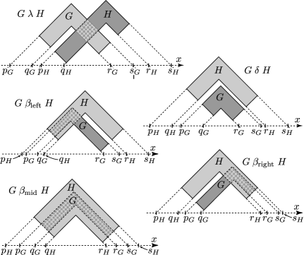
Figure 6. Possible positions of two illuminated sets in the plane

Definition 4.2.

Extending Czédli and Grätzer [7, Definition 4.1.(iii)] and Czédli [3, (4.1)], we define the following relations for $G,H\in\textup{LitSet}(L)$; see Figure 6 for illustrations.

• $G\mathrel{\lambda}H$, that is, $G$ is to the left of $H$ if $q_{G}\leq p_{H}$ and $s_{G}\leq r_{H}$;

• $G\mathrel{\delta}H$, that is, $G$ is geometrically under $H$ if $q_{H}\leq p_{G}$ and $s_{G}\leq r_{H}$;

• $G\mathrel{\beta_{\textup{mid}}}H$ if $p_{H}<p_{G}<q_{G}<q_{H}<r_{H}<r_{G}<s_{G}<s_{H}$;

• $G\mathrel{\beta_{\textup{left}}}H$ if $p_{H}\leq p_{G}<q_{G}<q_{H}$, $s_{G}\leq r_{H}$, and $G$ is internal;

• $G\mathrel{\beta_{\textup{right}}}H$ if $q_{H}\leq p_{G}$, $r_{H}<r_{G}<s_{G}\leq s_{H}$, and $G$ is internal.

Furthermore, for $I,J\in\textup{Lamp}(L)$, let $I\mathrel{\lambda}J$, $I\mathrel{\delta}J$, $I\mathrel{\beta_{\textup{mid}}}J$, $I\mathrel{\beta_{\textup{left}}}J$, and $I\mathrel{\beta_{\textup{right}}}J$ mean that $\textup{Lit}(I)\mathrel{\lambda}\textup{Lit}(J)$, $\textup{Lit}(I)\mathrel{\delta}\textup{Lit}(J)$, $\textup{Lit}(I)\mathrel{\beta_{\textup{mid}}}\textup{Lit}(J)$, $\textup{Lit}(I)\mathrel{\beta_{\textup{left}}}\textup{Lit}(J)$, and $\textup{Lit}(I)\mathrel{\beta_{\textup{right}}}\textup{Lit}(J)$, respectively.

The notations $\mathrel{\lambda}$ and $\mathrel{\delta}$ come from “Left” and “unDer”, respectively. Clearly,

$$\mathrel{\lambda} \mathrel{\delta}$$ and are irreflexive and transitive relations. (4.5)

Lemma 4.3.

Let $L$ be a slim rectangular lattice. Let $I$ and $J$ be either two distinct members of $\textup{Lamp}(L)$ or two distinct members of $\textup{LitSet}(L)$. Then exactly one of the following ten alternatives hold.

1. $I\mathrel{\lambda}J$,

2. $J\mathrel{\lambda}I$ (that is, $I$ is to the right of $J$, which is sometimes denoted by $I\mathrel{\rho}J$.)

3. $I\mathrel{\delta}J$,

4. $J\mathrel{\delta}I$,

5. $I\mathrel{\beta_{\textup{mid}}}J$,

6. $J\mathrel{\beta_{\textup{mid}}}L$

7. $I\mathrel{\beta_{\textup{left}}}J$,

8. $J\mathrel{\beta_{\textup{left}}}I$,

9. $I\mathrel{\beta_{\textup{right}}}J$,

10. $J\mathrel{\beta_{\textup{right}}}I$.

Furthermore, if $I$ and $J$ are incomparable in the poset $(\textup{Lamp}(L);\leq)$ or in the poset $(\textup{LitSet}(L);\leq)$, then the first four options are only possible.

Proof.

The internal illuminated sets are “A-shapes” (i.e., “V-shapes” turned upside down) with thickness or stripes. Those possible mutual geometric positions of two A-shapes that are not listed in the lemma are ruled out by Lemma 3.8 of [3]. If one of (v),…,(x) holds, then $(I,J)$ or $(J,I)$ belongs to ${{\rho}}_{\textup{foot}}$ and $I$ and $J$ are comparable by Lemma 2.2. Therefore, only (i), …, (iv) are allowed if $I$ and $J$ are incomparable. ∎

Definition 4.4.

Next, assume that we partition a rectangle into finitely many stripes by lines of slope $3\pi/4$; these stripes will be called abstract left boundary illuminated sets. Similarly, we partition the same rectangle into finitely many stripes by lines of slope $\pi/4$ to obtain the abstract right boundary illuminated sets. Then we add finitely many A-shapes called abstract internal illuminated sets such that

1. Lemma 4.3 holds for these abstract sets,

2. For any abstract boundary illuminated set $Z$, the condition formulated in (4.3) (and Lemma 3.9) of Czédli [3] is satisfied.

Then we say the our finite collection of abstract illuminated sets is an abstract illuminated system.

Two such systems are called similar if there is a bijective correspondence $\varphi$ between them such that both $\varphi$ and $\varphi^{-1}$ preserve each of the five relations described in Definition 4.2.

For $I\in\textup{Lamp}(L)$, $\textup{Floor}(I)$, $\textup{Roof}(I)$, $\textup{Foot}(I)$ and $\textup{Peak}(I)$ are determined by $\textup{Lit}(I)$. This allows us to define these objects, in a natural way, for $H\in\textup{LitSet}(L)$. Then, also, ${{\rho}}_{\textup{foot}}$ and ${{\rho}}_{\textup{infoot}}$ are defined on $\textup{LitSet}(L)$ and they are equal. (If their equality is not a consequence of definitions, then it should be added to Definition 4.4 as $(\#3)$.)

Definition 4.5.

An abstract illuminated system $\mathcal{S}$ is also a poset $\mathcal{S}:=(\mathcal{S};\leq)$ where “$\leq$” is the reflexive transitive closure of (4.4).

Comparing (4.4) to Definition 4.5 and using (2.3) and Lemma 4.1, we obtain the validity of the following lemma.

Lemma 4.6.

Let $D$ be a finite distributive lattice. If $D$ is representable as $\operatorname{Con}K$ for an SPS lattice $K$, then

1. there is an abstract illuminated system $(\mathcal{S};\leq)$ isomorphic to $(\textup{J}(D);\leq)$ and

2. there is a slim rectangular lattice $L$ such that $(\textup{LitSet}(L);\leq)$ is similar to the above-mentioned $(\mathcal{S};\leq)$.

We conjecture that Condition (i) of this lemma is not only a necessary but also a sufficient condition of the representability of $D$. If this is so, then the algorithm below becomes faster. But even though we do not prove this conjecture, Lemma 4.6 together with other known facts lead to the following algorithm.

Algorithm 4.7.

Assume that $D$ is a finite distributive lattice to be represented as the congruence lattice of an SPS (=slim semimodular) lattice. By (2.3), we can assume that this SPS lattice is a slim rectangular lattice $L$; see also (2.2) (If this $L$ exists, then the algorithm will construct it.) Let $n:=|\textup{J}(D)|$. We are going to find an abstract illuminated system $\mathcal{S}$ such that $(\mathcal{S};\leq)$ isomorphic to $(\textup{J}(D);\leq)$. Even if there are continuously many $n$-element abstract illuminated systems, we are only interested in $\mathcal{S}$ up to similarity. Any $n$-element abstract illuminated system is described by $n$ coordinate quadruples. Although the entries of these quadruples are real numbers (of which there are too many), the system up to similarity is determined by how these entries are ordered. Therefore, we can fix a $4n$-element set $U$ of real numbers such that each of the $n$ coordinate tuples belongs to $U^{4}$. Note, however, that when we use the algorithm (without computers), then we draw figures rather than paying attention to any $U$; $U$ is only mentioned here because its finiteness indicates that we are describing an algorithm.

We only list those abstract illuminated systems that, according to our theoretical knowledge, might be isomorphic to $(\textup{J}(D);\leq)$. First, by Czédli [3, Lemma 3.2], there should be exactly $|\textup{Max}(\textup{J}(D))|$ many boundary illuminated sets (that is, stripes) since they correspond to the maximal elements of $\textup{J}(D)$. Second, when deciding which of these $|\textup{Max}(\textup{J}(D))|$ many boundary illuminated sets should be on left and which on the right, we take the Bipartite Maximal Elements Property of Czédli [3, Corollary 3.4] into account. Either in the meantime or at the beginning, it is reasonable to check if $(\textup{J}(D);\leq)$ satisfies the seven previously known properties; see Czédli [3] and Czédli and Grätzer [7] where these properties are (first) proved or cited from Grätzer [20] and [21]. The properties occurring in the present paper are also useful as well as the known properties of lamps (translated to illuminated sets) are also useful since they exclude lots of case; see, Section 5 for some properties of lamps.

After parsing all the cases “permitted by known properties”, we can decide if there exists an abstract illuminated system $\mathcal{S}$ such that $(\mathcal{S};\leq)$ is isomorphic to $(\textup{J}(D);\leq)$. If such an $\mathcal{S}$ does not exists, then $D$ cannot be represented in the required way and the algorithm concludes with “no”. If $\mathcal{S}$ exists and the conjecture right after Lemma 4.6 is true, then the algorithm concludes with a positive answer.

If $\mathcal{S}$ exists but either we do not know whether the conjecture is true or we need to construct $D$, then we can do the following. Based on $\mathcal{S}$ (and slightly modifying it to a similar system from time to time when we bump into obstacles), we try to construct $D$; indeed, $\mathcal{S}$ serves as an outline and a bird’s-eye view of $D$. If we succeed, the algorithm concludes with “yes” and $L$ is also found. Otherwise, we try to construct $D$ from another $\mathcal{S}$. If, after constructing all $\mathcal{S}$ with $(\mathcal{S},\leq)\cong(\textup{J}(D);\leq)$ but failing to construct $L$ from them, the algorithm yields a negative answer.

5. Some easy lemmas about lamps

In this section, as a preparation for Sections 6 and 7, we prove some easy statements.

Lemma 5.1.

If $L$ is as in (2.2), $I,J\in\textup{Lamp}(L)$, and $I$ is geometrically under $I$ (in notation, $I\mathrel{\delta}J$), then $I\nprec J$ in $\textup{Lamp}(L)$. Equivalently, if and $I\prec J$ in $\textup{Lamp}(L)$, then $I\mathrel{\delta}J$ cannot hold.

Proof.

Suppose the contrary. Then $I\mathrel{\delta}J$ and, by Lemma 2.2, $(I,J)\in{{\rho}}_{\textup{Body}}$. Since $I\mathrel{\delta}J$, $\textup{Lit}(I)$ and $\textup{Lit}(J)$ are sufficiently disjoint in the sense of (3,4) of Czédli [3], contradicting $(I,J)\in{{\rho}}_{\textup{Body}}$. ∎

For $U\in\textup{Lamp}(L)$, let $\mathord{\downarrow_{\textup{g}}}\textup{Roof}(U)$ denote the set of those geometric points of the full geometric rectangle (of the $\mathcal{C}_{1}$-diagram of $L$) that are on or below $\textup{Roof}(U)$. More precisely, a geometric point $(x,y)$ (given in the usual coordinate system) of the full geometric rectangle belongs to $\mathord{\downarrow_{\textup{g}}}\textup{Roof}(U)$ if and only if $(x,y^{\prime})\in\textup{Roof}(U)$ for some $y^{\prime}$ such that $y^{\prime}\geq y$.

Lemma 5.2.

If $L$ is from (2.2) and $I<J$ holds in $\textup{Lamp}(L)$, then $\mathord{\downarrow_{\textup{g}}}\textup{Roof}(I)\subseteq\mathord{\downarrow_{\textup{g}}}\textup{Roof}(J)$.

Proof.

If $I\prec J$, then $(I,J)\in{{\rho}}_{\textup{Body}}$ by Lemma 2.2, whence $\textup{Body}(I)\subseteq\mathord{\downarrow_{\textup{g}}}\textup{Roof}(J)$ gives the required inclusion $\mathord{\downarrow_{\textup{g}}}\textup{Roof}(I)\subseteq\mathord{\downarrow_{\textup{g}}}\textup{Roof}(J)$. Otherwise, the inclusion follows from its just-mentioned particular case by transitivity. ∎

Next, we prove the following lemma; the conjunction of this lemma with Lemma 4.3 is stronger than Czédli and Grätzer [7, Lemma 4.3].

Lemma 5.3.

For $L$ from (2.2) and $I,J,K\in\textup{Lamp}(L)$, if $I\mathrel{\delta}J$ and $K<I$, then $K\nprec J$. That is, if $I$ is geometrically under $J$, then no element of the principal ideal $\mathord{\downarrow}\kern 0.5ptI$ is covered by $J$ in $\textup{Lamp}(L)$.

Proof.

Assume that $I\mathrel{\delta}J$ and $K\leq I$. Lemma 5.2 gives that $\mathord{\downarrow_{\textup{g}}}\textup{Roof}(K)\subseteq\mathord{\downarrow_{\textup{g}}}\textup{Roof}(I)$. Hence, $\textup{Foot}(K)\in\mathord{\downarrow_{\textup{g}}}\textup{Roof}(I)$. Actually, $\textup{Foot}(K)\in\textup{GInt}(\mathord{\downarrow_{\textup{g}}}\textup{Roof}(I))$ since at least one precipitous edge going upwards starts at or above $\textup{Foot}(K)$. Since $I\mathrel{\delta}J$, $\textup{GInt}(\mathord{\downarrow_{\textup{g}}}\textup{Roof}(I))\cap\textup{GInt}(\textup{Lit}(J))=\emptyset$. Hence, $\textup{Foot}(K)\notin\textup{GInt}(\textup{Lit}(J))$, that is, $(K,J)\notin{{\rho}}_{\textup{infoot}}$. Therefore, the required $K\nprec J$ follows by Lemma 2.2. ∎

Lemma 5.4.

If $L$ is from (2.2), $I,J,K\in\textup{Lamp}(L)$, $J\mathrel{\delta}K$, and $I\leq J$, then $I\mathrel{\delta}K$.

Proof.

Apply Lemma 5.2. ∎

Yet we state another easy lemma. For an illustration, see Figure 8 in Czédli and Grätzer [7].

Lemma 5.5.

Assume that $L$ is from (2.2), $A_{0}$, $A_{1}$, $A_{2}$ and $B_{1}$ are from $\textup{Lamp}(L)$, $A_{0}\mathrel{\lambda}A_{1}\mathrel{\lambda}A_{2}$, $B_{1}\prec A_{0}$, and $B_{1}\prec A_{2}$. Then $B_{1}\mathrel{\delta}A_{1}$.

Proof.

By Lemma 2.2, $(B_{1},A_{0}),(B_{1},A_{2})\in{{\rho}}_{\textup{Body}}$. Hence $\textup{Body}(B_{1})\subseteq\textup{Lit}(A_{0})\cap\textup{Lit}(A_{2})$, see Czédli and Grätzer [7, Figure 8], and we obtain that $B_{1}\mathrel{\delta}A_{1}$. ∎

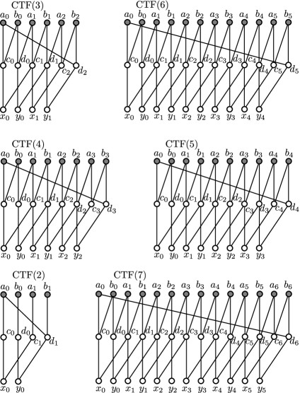
Figure 7. The posets $\textup{CTF}(2)$, …, $\textup{CTF}(7)$

6. An infinite family of new properties of congruence lattices of SPS lattices

For an integer $n\geq 2$, we define the poset Crown with Two Fences of order $n$, in notation $\textup{CTF}(n)$ as follows; see also Figure 7. The elements of $\textup{CTF}(n)$ are $a_{0}$, $a_{1}$, …, $a_{n-1}$, $b_{0}$, $b_{1}$, …, $b_{n-1}$, $c_{0}$, $c_{1}$, …, $c_{n-1}$, $d_{0}$, $d_{1}$, …, $d_{n-1}$, $x_{0}$, $x_{1}$, …, $x_{n-2}$, and $y_{0}$, $y_{1}$, …, $y_{n-2}$; they are pairwise distinct. The edges (in other words, the prime intervals) are as follows, the arithmetic in the subscripts is understood on $\mathbb{Z}_{n}$, that is, modulo $n$: $c_{i}\prec a_{i}$ and $c_{i}\prec b_{i}$ for $i\in\mathbb{Z}_{n}$, $d_{i}\prec b_{i}$ and $d_{i}\prec a_{i+1}$ for $i\in\mathbb{Z}_{n}$, $x_{j}\prec c_{j}$ and $x_{j}\prec c_{j+1}$ for $j\in\{0,1,\dots,n-2\}$, and $y_{j}\prec d_{j}$ and $y_{j}\prec d_{j+1}$ for $j\in\{0,1,\dots,n-2\}$. In the figure, the maximal elements of $\textup{CTF}(n)$ are grey-filled.

For posets $P_{1}$, $P_{2}$ and a map (ALSO KNOWN AS function) $\varphi\colon P_{1}\to P_{2}$, we say that $\varphi$ is an embedding if

for any $$x,y\in P_{1} x\leq y P_{1} \varphi(x)\leq\varphi(y) P_{2}$$,   in if and only if in . (6.1)

If $\varphi\colon P_{1}\to P_{2}$ is an embedding and, in addition,

for any $$x,y\in P_{1} x\prec y P_{1} \varphi(x)\prec\varphi(y) P_{2}$$,   in if and only if in , (6.2)

then $\varphi$ is called a cover-preserving embedding. Finally, if $\varphi\colon P_{1}\to P_{2}$ is an embedding such that $\varphi(x)$ is a maximal element of $P_{2}$ for every maximal element $x\in P_{1}$, then $\varphi$ is a maximum-preserving embedding. By an SPS lattice we still mean a slim semimodular lattice.

Definition 6.1.

For an integer $n\geq 2$ and a poset $P$, we say that $P$ satisfies the $\textup{CTF}(n)$-property if there exists no cover-preserving embedding $\varphi\colon\textup{CTF}(n)\to P$ that is also maximum-preserving.

Theorem 6.2.

For every integer $n\geq 2$ and any SPS lattice $K$, $\textup{J}(\operatorname{Con}K)$ satisfies the $\textup{CTF}(n)$-property.

Proof.

By way of contradiction, suppose that the theorem fails for some $n\geq 2$. By Lemma 2.2(ii), $(\textup{J}(L);\leq)\cong(\textup{Lamp}(L);\leq)$ for a slim rectangular lattice $L$. Hence, there is a maximum-preserving and cover-preserving embedding $\varphi\colon\textup{CTF}(n)\to\textup{Lamp}(L)$; for $x\in\textup{CTF}(n)$, we denote $\varphi(x)$ by the corresponding capital letter, $X$. By left-right symmetry and the Bipartite Maximal Elements Property, see Czédli [3, Lemma 3.4], we can assume that $A_{0},\dots,A_{n-1}$ are left boundary lamps while $B_{0},\dots,B_{n-1}$ are right boundary lamps. (There can be other boundary lamps but they are not $\varphi$-images and cause no trouble.) Let $A_{i}\mathrel{\lambda_{\textup{bnd}}}A_{j}$ mean that $A_{i}$ is to the left of $A_{j}$ on the left upper boundary of $L$. Similarly, $B_{i}\mathrel{\lambda_{\textup{bnd}}}B_{j}$ means that $B_{i}$ is to the left of $B_{j}$ on the right upper boundary of $L$. We know from (i) and (iii) of Lemma 2.2 that

if $$x\prec y \textup{CTF}(n) (X,Y)\in{{\rho}}_{\textup{Body}} \textup{Body}(X)\subseteq\textup{Lit}(Y)$$ in , then and so . (6.3)

We claim that

$$\text{for $i\in\{0,1,\dots,n-2\}$, if $A_{i}\mathrel{\lambda_{\textup{bnd}}}A_{i+1}$, then $B_{i}\mathrel{\lambda_{\textup{bnd}}}B_{i+1}$}.$$ (6.4)

We prove this by way of contradiction. Suppose that $A_{i}\mathrel{\lambda_{\textup{bnd}}}A_{i+1}$ holds but $B_{i}\mathrel{\lambda_{\textup{bnd}}}B_{i+1}$ fails. Then $B_{i+1}\mathrel{\lambda_{\textup{bnd}}}B_{i}$. Since we know from (6.3) that $\textup{Body}(C_{i})\in\textup{Lit}(A_{i})\cap\textup{Lit}(B_{i})$ and $\textup{Body}(C_{i+1})\in\textup{Lit}(A_{i+1})\cap\textup{Lit}(B_{i+1})$, we obtain that $C_{i}\mathrel{\delta}C_{i+1}$. In virtue of Lemma 5.3, $C_{i}\mathrel{\delta}C_{i+1}$ and $X_{i}<C_{i}$ implies that $X_{i}\nprec C_{i+1}$. This is a contradiction since $\varphi$ is cover-preserving. We have proved (6.4).

Next, we claim that

$$\text{for $i\in\{0,1,\dots,n-2\}$, if $B_{i}\mathrel{\lambda_{\textup{bnd}}}B_{i+1}$, then $A_{i+1}\mathrel{\lambda_{\textup{bnd}}}A_{i+2}$};$$ (6.5)

here $i+2$ is understood in $\mathbb{Z}_{n}$, that is, $(n-2)+2=0$. To prove (6.5) by way of contradiction, suppose that $B_{i}\mathrel{\lambda_{\textup{bnd}}}B_{i+1}$ but $A_{i+2}\mathrel{\lambda_{\textup{bnd}}}A_{i+1}$. Then, similarly to the argument given for (6.4), (6.3) yields that $D_{i+1}\mathrel{\delta}D_{i}$. Using $D_{i+1}\mathrel{\delta}D_{i}$, $Y_{i}<D_{i+1}$, and $Y_{i}\prec D_{i}$, Lemma 5.3 gives a contradiction and proves (6.5).

Clearly, either $A_{0}\mathrel{\lambda_{\textup{bnd}}}A_{1}$ or $A_{1}\mathrel{\lambda_{\textup{bnd}}}A_{0}$ (that is, $A_{0}\mathrel{\rho}A_{1}$, see Lemma 4.3(ii)). By symmetry, (6.4) and (6.5) also hold for $\mathrel{\rho}$. Thus, we can assume that $A_{0}\mathrel{\lambda_{\textup{bnd}}}A_{1}$, and we can argue as follows; when referencing (6.4) or (6.5) over implication signs, the value of $i$ will be indicated. We obtain that

$$\left.\begin{aligned} A_{0}\mathrel{\lambda_{\textup{bnd}}}A_{1}&\overset{(\ref{eq:csnkrnkcsJr},i=0)}{\Longrightarrow}B_{0}\mathrel{\lambda_{\textup{bnd}}}B_{1}\overset{(\ref{eq:nhnmgdhGmtDd},i=0)}{\Longrightarrow}A_{1}\mathrel{\lambda_{\textup{bnd}}}A_{2}\overset{(\ref{eq:csnkrnkcsJr},i=1)}{\Longrightarrow}B_{1}\mathrel{\lambda_{\textup{bnd}}}B_{2}\cr&\overset{(\ref{eq:nhnmgdhGmtDd},i=1)}{\Longrightarrow}A_{2}\mathrel{\lambda_{\textup{bnd}}}A_{3}\overset{(\ref{eq:csnkrnkcsJr},i=2)}{\Longrightarrow}B_{2}\mathrel{\lambda_{\textup{bnd}}}B_{3}\overset{(\ref{eq:nhnmgdhGmtDd},i=3)}{\Longrightarrow}A_{3}\mathrel{\lambda_{\textup{bnd}}}A_{4}\text{ }\dots\cr&\dots\text{ }A_{n-2}\mathrel{\lambda_{\textup{bnd}}}A_{n-1}\cr&\overset{(\ref{eq:csnkrnkcsJr},i=n-2)}{\Longrightarrow}B_{n-2}\mathrel{\lambda_{\textup{bnd}}}B_{n-1}\overset{(\ref{eq:nhnmgdhGmtDd},i=n-2)}{\Longrightarrow}A_{n-1}\mathrel{\lambda_{\textup{bnd}}}A_{0}.\end{aligned}\,\,\right\}$$ (6.6)

By the first three lines of (6.6) and the transitivity of $\mathrel{\lambda_{\textup{bnd}}}$, we have that $A_{0}\mathrel{\lambda_{\textup{bnd}}}A_{n-1}$. But this contradicts the last line of (6.6), where $A_{n-1}\mathrel{\lambda_{\textup{bnd}}}A_{0}$. The proof of Theorem 6.2 is complete. ∎

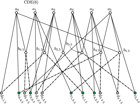
Figure 8. $\textup{CDE}(6)$

7. Another infinite family of new properties

Following Czédli and Schmidt [14], patch lattices are slim rectangular lattices in which the corners are coatoms. These lattices have only two boundary lamps. Hence, if $L$ is a slim patch lattice, then $\textup{J}(\operatorname{Con}L)$ only has two maximal elements, whereby $\textup{J}(\operatorname{Con}L)$ trivially satisfies $\textup{CTF}(n)$ for all $n\geq 2$. This means that Theorem 6.2 says nothing on the congruence lattices of slim patch lattices. This observation motivates us to present another infinite family of properties; these properties are interesting even in the study of congruence lattices of slim patch lattices.

For an integer $n\geq 3$, we define the poset Crown with Diamonds and Emeralds of order $n$, denoted by $\textup{CDE}(n)$, as follows; note that $\textup{CDE}(6)$ is drawn in Figure 8. First, let

$$\frac{1}{2}\mathbb{Z}_{n}:=\{0,0.5,1,1.5,2,2.5,\dots,n-1,n-0.5\};$$

it is an additive abelian group and $\mathbb{Z}_{n}$ is one of its subgroups. That is, we perform the addition and subtraction in $\frac{1}{2}\mathbb{Z}_{n}$ modulo $n$. For example, in $\frac{1}{2}\mathbb{Z}_{4}$, we have that $2+2=0.5+3.5=0$ and $1-3.5=1.5$. The underlying set of our poset is

$$\textup{CDE}(n):=\{a_{i}:i\in\mathbb{Z}_{n}\} \cup\{b_{i+0.5}:i\in\mathbb{Z}_{n}\}$$

$$\cup\{d_{i,i+1.5}:i\in\mathbb{Z}_{n}\}\cup\{e_{i,i-1.5}:i\in\mathbb{Z}_{n}\}$$

while its edges (that is, prime intervals) are $b_{i-0.5}\prec a_{i}$, $b_{i+0.5}\prec a_{i}$, $d_{i,i+1.5}\prec a_{i}$, $d_{i,i+1.5}\prec b_{i+1.5}$, $e_{i,i-1.5}\prec a_{i}$, and $d_{i,i-1.5}\prec b_{i-1.5}$, for $i\in\mathbb{Z}_{n}$; see Figures 8 and 9 for illustration. The elements of the forms $a_{i}$, $b_{i}$, $d_{i,i+1.5}$, and $e_{i,i-1.5}$ of $\textup{CDE}(n)$ are called maximal elements, atoms, diamonds, and emeralds, respectively. Note that $|\textup{CDE}(n)|=4n$.

For a poset $P$ and an embedding $\varphi\colon(\textup{CDE}(n);\leq)\to(P;\leq)$, we say that $\varphi$ preserves the coatomic edges if whenever $x\prec y$ in $\textup{CDE}(n)$ and $y$ is a maximal element (that is, $y$ is of the form $a_{i}$), then $\varphi(x)\prec\varphi(y)$ in $P$. For example, any cover-preserving embedding $\textup{CDE}(n)\to P$ preserves the coatomic edges but not conversely. We say that an order-preserving function $\varphi\colon(\textup{CDE}(n);\leq)\to(P;\leq)$ is a de-embedding if its restriction to $\textup{CDE}(n)\setminus\{$diamonds$\}$ and its restriction to $\textup{CDE}(n)\setminus\{$emeralds$\}$ are order embeddings.

Definition 7.1.

For an integer $n\geq 3$, we say that a poset $P$ satisfies the $\textup{CDE}(n)$-property if there exists no de-embedding $\varphi\colon\textup{CDE}(n)\to P$ preserving the coatomic edges.

Note that for $n=6$, the condition on $\varphi$ is visualized in Figure 8 as follows: $\varphi$ has to preserve the coverings denoted by thin solid edges but it need not preserve the coverings indicated by the somewhat thicker “dash-dot-dash-dot”-drawn edges. Let us emphasize that if $\varphi\colon(\textup{CDE}(n);\leq)\to(P;\leq)$ preserves the coatomic edges, then the $\varphi$-images of the maximal elements of $\textup{CDE}(n)$ need not be maximal in $P$. By an SPS lattice we still mean a slim semimodular lattice (which is necessarily planar).

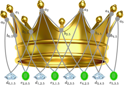
Figure 9. Motivating the terminology by a subposet of $\textup{CDE}(9)$

Theorem 7.2.

For every integer $n\geq 3$ and any SPS lattice $K$, $\textup{J}(\operatorname{Con}K)$ satisfies the $\textup{CDE}(n)$-property.

Proof of Theorem 7.2.

To present a proof by way of contradiction, suppose that the theorem fails. By Lemma 2.2(ii), $(\textup{J}(L);\leq)\cong(\textup{Lamp}(L);\leq)$ for a slim rectangular lattice $L$. Hence, there is de-embedding $\varphi\colon\textup{CDE}(n)\to\textup{Lamp}(L)$ that preserves the coatomic edges. Again, for $x\in\textup{CDE}(n)$, $X:=\varphi(x)$. The disjunction of $A_{i_{1}}\mathrel{\lambda}A_{i_{2}}$ and $A_{i_{2}}\mathrel{\lambda}A_{i_{1}}$ is denoted by $A_{i_{1}}\mathrel{\parallel_{\textup{g}\lambda\rho}}A_{i_{2}}$. (The subscript comes from “geometrically left or right”.) For $i\in\mathbb{Z}_{n}$, $A_{i}$ and $A_{i+1}$ have a common lower cover, $B_{i+0.5}\in\textup{Lamp}(L)$. (Here and later, the arithmetics for indices is understood in $\frac{1}{2}\mathbb{Z}_{n}$, that is, modulo $n$.) By Lemma 4.3 of Czédli and Grätzer [7] (or by Lemma 5.3 and the last sentence of Lemma 4.3),

for every $$i\in\mathbb{Z}_{n} A_{i}\mathrel{\parallel_{\textup{g}\lambda\rho}}A_{i+1}$$, . (7.1)

Next, we claim that

for every $$i\in\mathbb{Z}_{n} A_{i}\mathrel{\lambda}A_{i+1} A_{i+1}\mathrel{\lambda}A_{i+2}$$, if , then . (7.2)

To show this, suppose the contrary. Then, by (7.1), $A_{i}\mathrel{\lambda}A_{i+1}$ and $A_{i+2}\mathrel{\lambda}A_{i+1}$. For the geometric relation between $A_{i}$ and $A_{i+2}$, the (last sentence of) Lemma 4.3 only allows four possibilities; we are going the exclude each of these four possibilities and then (7.2) will follow by way of contradiction.

First, let $A_{i+2}\mathrel{\delta}A_{i}$. Then Lemma 5.3 applies since $A_{i+2}\mathrel{\delta}A_{i}$, $D_{i,i+1.5}<B_{i+1.5}\prec A_{i+2}$, and we obtain that $D_{i,i+1.5}\nprec A_{i}$, a contradiction.

Second, let $A_{i}\mathrel{\delta}A_{i+2}$. Then Lemma 5.3 applies to $A_{i}\mathrel{\delta}A_{i+2}$ and $E_{i+2,i+0.5}<B_{i+0.5}\prec A_{i}$, and we get a contradiction, $E_{i+2,i+0.5}\nprec A_{i+2}$.

Third, let $A_{i}\mathrel{\lambda}A_{i+2}$. Then $A_{i}\mathrel{\lambda}A_{i+2}\mathrel{\lambda}A_{i+1}$, $B_{i+0.5}\prec A_{i}$, and $B_{i+0.5}\prec A_{i+1}$. Hence, Lemma 5.5 implies that $B_{i+0.5}\mathrel{\delta}A_{i+2}$. Now $B_{i+0.5}\mathrel{\delta}A_{i+2}$,   $E_{i+2,i+0.5}<B_{i+0.5}$, and Lemma 5.3 give that $E_{i+2,i+0.5}\nprec A_{i+2}$, a contradiction again.

Fourth, let $A_{i+2}\mathrel{\lambda}A_{i}$. Then $A_{i+2}\mathrel{\lambda}A_{i}\mathrel{\lambda}A_{i+1}$,  $B_{i+1.5}\prec A_{i+2}$,   $B_{i+1.5}\prec A_{i+1}$, and Lemma 5.5 give that $B_{i+1.5}\mathrel{\delta}A_{i}$. Hence, $B_{i+1.5}\mathrel{\delta}A_{i}$, $D_{i,i+1.5}<B_{i+1.5}$, and Lemma 5.3 imply that $D_{i,i+1.5}\nprec A_{i}$, which is a contradiction. We have verified (7.2).

Finally, using (7.1) and reflecting the diagram across a vertical axis if necessary, we can assume that $A_{0}\mathrel{\lambda}A_{1}$. Then, keeping in mind that $(n-1)+1=0$ in $\mathbb{Z}_{n}$ and using (7.2) repeatedly, we obtain that

$$A_{0}\mathrel{\lambda}A_{1}\mathrel{\lambda}A_{2}\mathrel{\lambda}A_{3}\mathrel{\lambda}\dots\mathrel{\lambda}A_{n-1}\mathrel{\lambda}A_{0}.$$

By the transitivity of $\mathrel{\lambda}$, see (4.5), it follows that $A_{0}\mathrel{\lambda}A_{0}$, which is a contradiction since $\mathrel{\lambda}$ is irreflexive by (4.5). This completes the proof of Theorem 7.2. ∎

8. Concluding remarks

The $\textup{CTF}(2)$-property is the same as the Two-pendant Four-crown Property, see Definition 4.1 and Theorem 4.3 in Czédli [3].

A poset $P$ has the Three-pendant Three-crown property, see Czédli and Grätzer [7], if there is no cover-preserving embedding of $\textup{CDE}(3)\setminus\{e_{0,1.5},e_{1,2.5},e_{2,0.5}\}$ into $P$. Since the de-embedding need not be (fully) cover-preserving in Definition 7.1 and, in case of $\textup{CDE}(3)$, it can collapse each diamond with the emerald having the same subscript, the $\textup{CDE}(3)$-property is stronger than the Three-pendant Three-crown property. Indeed, it is a trivial task to add some new elements to $\textup{CDE}(3)$ to obtain a poset that satisfies the Three-pendant Three-crown property but fails to satisfy the $\textup{CDE}(3)$-property. Therefore, the $n=3$ instance of Theorem 7.2 is stronger than the main result of Czédli and Grätzer [7].

The smallest instance of the $\textup{CTF}(n)$-property and that of the $\textup{CDE}(n)$-property have been analysed. Hence, in the rest of this section, we assume that $n\geq 3$ for the $\textup{CTF}(n)$-property and $n\geq 4$ for the $\textup{CDE}(n)$-property even if this will not be mentioned explicitly.

For $k\geq 3$, let $D_{k}$ be the distributive lattice such that $\textup{J}(D_{k})\cong\textup{CTF}(k)$. Since crowns of different sizes cannot be embedded into each other, it is easy to see that $D$ satisfies the seven previously known properties, the $\textup{CTF}(n)$-properties for all $n\neq k$, and the $\textup{CDE}(n)$-properties for all $n\geq 3$. However, $\textup{CTF}(k)$ fails in $D_{k}$. Similarly, if $k\geq 4$ and $D^{\prime}_{k}$ is the distribute lattice defined by $\textup{J}(D^{\prime}_{k})\cong\textup{CDE}(k)$, then $D^{\prime}_{k}$ satisfies the seven previously known properties, the $\textup{CDE}(n)$-properties for all $n\neq k$, and the $\textup{CTF}(n)$-properties for all $n\geq 3$. Therefore, the $\textup{CTF}(n)$-properties, for $n\geq 3$ and the $\textup{CDE}(n)$-properties, for $n\geq 4$ are new and we have an independent infinite set of properties of congruence lattice of SPS lattices.

The injectivity of $\varphi$ means a plenty of conditions of the pattern “if $x\neq y$ then $\varphi(x)\neq\varphi(y)$”. Observing that not all of these conditions are used in our proofs, it is possible to strengthen the new properties given in the paper and even some of the old properties. These details are elaborated in Czédli [5].

References

- [1] Czédli, G.: Patch extensions and trajectory colorings of slim rectangular lattices. Algebra Universalis 72, 125–154 (2014)
- [2] Czédli, G.: Diagrams and rectangular extensions of planar semimodular lattices. Algebra Universalis 77, 443–498 (2017)
- [3] Czédli, G.: Lamps in slim rectangular planar semimodular lattices. Acta Sci. Math. (Szeged) 87, 381–413 (2021) (Open access: https://doi.org/10.14232/actasm-021-865-y)
- [4] Czédli, G.: Non-finite axiomatizability of some finite structures. Archivum Mathematicum Brno 58, 15–33 (2022)
- [5] Czédli, G.: Infinitely many new properties of the congruence lattices of slim semimodular lattices. In preparation (to be submitted to a journal very soon)
- [6] Czédli, G., Dékány, T., Gyenizse, G., Kulin, J.: The number of slim rectangular lattices. Algebra Universalis 75, 33–50 (2016)
- [7] Czédli, G., Grätzer, G.: A new property of congruence lattices of slim, planar, semimodular lattices. Categories and General Algebraic Structures with Applications 16, 1-28 (2022) (Open access: https://cgasa.sbu.ac.ir/article_101508.html)
- [8] Czédli, G., Grätzer, G., Lakser, H.: Congruence structure of planar semimodular lattices: The General Swing Lemma. Algebra Universalis 79:40 (2018)
- [9] Czédli, G., Kurusa, Á.: A convex combinatorial property of compact sets in the plane and its roots in lattice theory. Categories and General Algebraic Structures with Applications 11, 57–92 (2019) http://cgasa.sbu.ac.ir/article_82639.html
- [10] Czédli, G., Makay, G.: Swing lattice game and a direct proof of the swing lemma for planar semimodular lattices. Acta Sci. Math. (Szeged) 83, 13–29 (2017)
- [11] Czédli, G., Ozsvárt, L., Udvari, B.: How many ways can two composition series intersect?. Discrete Mathematics 312, 3523–3536 (2012)
- [12] Czédli, G., Schmidt, E. T.: The Jordan-Hölder theorem with uniqueness for groups and semimodular lattices. Algebra Universalis 66, 69–79 (2011)
- [13] Czédli, G., Schmidt, E. T.: Slim semimodular lattices. I. A visual approach. Order 29, 481–497 (2012)
- [14] Czédli, G., Schmidt, E. T.: Slim semimodular lattices. II. A description by patchwork systems. ORDER 30, 689–721 (2013)
- [15] Day, A.: Characterizations of finite lattices that are bounded-homomorphic images or sublattices of free lattices. Canad. J. Math. 31, 69–78 (1979)
- [16] Freese, R., Ježek, J., Nation, J. B.: Free lattices. Mathematical Surveys and Monographs, 42, American Mathematical Society, Providence, RI, (1995)
- [17] Grätzer, G.: Lattice Theory: Foundation. Birkhäuser, Basel (2011)
- [18] Grätzer, G.: Congruences in slim, planar, semimodular lattices: The Swing Lemma. Acta Sci. Math. (Szeged) 81, 381–397 (2015)
-
[19]
Grätzer, G.:
The Congruences of a Finite Lattice, A Proof-by-Picture Approach,
second edition.
Birkhäuser, 2016. xxxii+347. Part I is accessible at
https://www.researchgate.net/publication/299594715 - [20] Grätzer, G.: Congruences of fork extensions of slim, planar, semimodular lattices. Algebra Universalis 76, 139–154 (2016)
- [21] Grätzer, G.: Notes on planar semimodular lattices. VIII. Congruence lattices of SPS lattices. Algebra Universalis 81 (2020), Paper No. 15, 3 pp.
- [22] Grätzer, G., Knapp, E.: Notes on planar semimodular lattices. I. Construction. Acta Sci. Math. (Szeged) 73, 445–462 (2007)
- [23] G. Grätzer and E. Knapp, Notes on planar semimodular lattices. III. Rectangular lattices. Acta Sci. Math. (Szeged) 75 (2009), 29–48.
- [24] Kelly, D., Rival, I.: Planar lattices. Canad. J. Math. 27, 636–665 (1975)