Verified Causal Broadcast with Liquid Haskell

Abstract.

Protocols to ensure that messages are delivered in causal order are a ubiquitous building block of distributed systems. For instance, distributed data storage systems can use causally ordered message delivery to ensure causal consistency, and CRDTs can rely on the existence of an underlying causally-ordered messaging layer to simplify their implementation. A causal delivery protocol ensures that when a message is delivered to a process, any causally preceding messages sent to the same process have already been delivered to it. While causal delivery protocols are widely used, verification of their correctness is less common, much less machine-checked proofs about executable implementations.

We implemented a standard causal broadcast protocol in Haskell and used the Liquid Haskell solver-aided verification system to express and mechanically prove that messages will never be delivered to a process in an order that violates causality. We express this property using refinement types and prove that it holds of our implementation, taking advantage of Liquid Haskell’s underlying SMT solver to automate parts of the proof and using its manual theorem-proving features for the rest. We then put our verified causal broadcast implementation to work as the foundation of a distributed key-value store.

1. Introduction

Causal message delivery (Birman and Joseph, 1987a; Schiper et al., 1989; Birman and Joseph, 1987b; Birman et al., 1991) is a fundamental communication abstraction for distributed computations in which processes communicate by sending and receiving messages. One of the challenges of implementing distributed systems is the asynchrony of message delivery; messages arriving at the recipient in an unexpected order can cause confusion and bugs. A causal delivery protocol can ensure that, when a message $m$ is delivered to a process $p$, any message sent “before” $m$ (in the sense of Lamport’s “happens-before”; see Section 2.1) will have already been delivered to $p$. When a mechanism for causal message delivery is available, it simplifies the implementation of many important distributed algorithms, such as replicated data stores that must maintain causal consistency (Ahamad et al., 1995; Lloyd et al., 2011), conflict-free replicated data types (Shapiro et al., 2011b), distributed snapshot protocols (Acharya and Badrinath, 1992; Alagar and Venkatesan, 1994), and applications that “involve human interaction and consist of large numbers of communication endpoints” (van Renesse, 1993). A particularly useful special case of causal delivery is causal broadcast, in which each message is sent to all processes in the system. For example, a causal broadcast protocol enables a straightforward implementation strategy for a causally consistent replicated data store — one of the strongest consistency models available for applications that must maximize availability and tolerate network partitions (Mahajan et al., 2011). Conflict-free replicated data types (CRDTs) implemented in the operation-based style (Shapiro et al., 2011b, a) typically also assume the existence of an underlying causal broadcast layer (Shapiro et al., 2011b, §2.4).

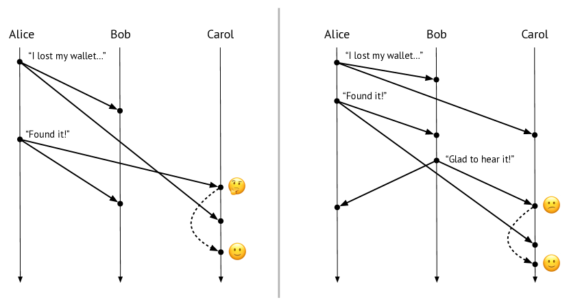
Figure 1. Two executions that violate causal delivery (Definition 2). On the left, Carol sees Alice’s messages in the opposite order of how they were sent. On the right, Carol sees Bob’s message before seeing Alice’s second message. The dashed arrows in both diagrams depict how a causal delivery mechanism (Section 2.2) might delay received messages in a buffer for later delivery.

What can go wrong in the absence of causal broadcast? Suppose Alice, Bob, and Carol are exchanging group text messages. Alice sends the message “I lost my wallet…” to the group, then finds the missing wallet between her couch cushions and follows up with a “Found it!” message to the group. In this situation, depicted in Figure 1 (left), Alice has a reasonable expectation that Bob and Carol will see the messages in the order that she sent them, and such first-in first-out (FIFO) delivery is an aspect of causal message ordering. While FIFO delivery is already enforced by standard networking protocols such as TCP (Postel, 1981), it is not enough to eliminate all violations of causality. In an execution such as that in Figure 1 (right), FIFO delivery is observed, and yet Carol sees Bob’s message only after having seen Alice’s initial “I lost my wallet…” message, so from Carol’s perspective, Bob is being rude. The issue is that Bob’s “Glad to hear it!” response causally depends on Alice’s second message of “Found it!”, yet Carol sees “Glad to hear it!” first. What is called for is a mechanism that will ensure that, for every message that is applied at a process, all of the messages on which it causally depends — comprising its causal history — are applied at that process first, regardless of who sent them.

One way to address the problem is to buffer messages at the receiving end until all causally preceding broadcast messages have been applied. The dashed arrows in Figure 1 represent the behavior of such a buffering mechanism. A typical implementation strategy is to have the sender of a message augment the message with metadata (for instance, a vector clock; see Section 2.2.1) that summarizes that message’s causal history in a way that can be efficiently checked on the receiver’s end to determine whether the message needs to be buffered or can be applied immediately to the receiver’s state. Although such mechanisms are well-known in the distributed systems literature (Birman and Joseph, 1987a, b; Birman et al., 1991), their implementation is “generally very delicate and error prone” (Bouajjani et al., 2017), motivating the need for machine-verified implementations of causal delivery mechanisms that are usable in real, running code.

To address this need, we use the Liquid Haskell (Vazou et al., 2014) platform to implement and verify the correctness of a well-known causal broadcast protocol (Birman et al., 1991). Liquid Haskell is an extension to the Haskell programming language that adds support for refinement types (Rushby et al., 1998; Xi and Pfenning, 1998), which let programmers specify logical predicates that restrict, or refine, the set of values described by a type. Beyond giving more precise types to individual functions, Liquid Haskell’s reflection (Vazou et al., 2017, 2018) facility lets programmers use refinement types to extrinsically specify properties that can relate multiple functions (see Section 3.2), and then prove those properties by writing Haskell programs to inhabit the specified types. We use this capability to prove that in our causal broadcast implementation, processes deliver messages in causal order, ruling out the possibility of causality-violating executions like those in Figure 1.

We express causal delivery as a refinement type. By doing so, we can take advantage of Liquid Haskell’s underlying SMT automation where possible, while still availing ourselves of the full power of Liquid Haskell’s theorem-proving capabilities via reflection where necessary. A further advantage of Liquid Haskell as a verification platform is that it results in immediately executable Haskell code, with no extraction step necessary, as with proof assistants such as Coq (Bertot and Castéran, 2004) or Isabelle (Wenzel et al., 2008) — making it easy to integrate our library with existing Haskell code.

Our causal broadcast implementation is a Haskell library that can be used in a variety of applications. While previous work has mechanically verified the correctness of applications of causal ordering in distributed systems (such as causally consistent distributed key-value stores (Lesani et al., 2016; Gondelman et al., 2021)), factoring the causal broadcast protocol out into its own standalone, verified component means that it can be reused in each of these contexts. There is a need for such a standalone component: for instance, recent work on mechanized verification of CRDT convergence (Gomes et al., 2017) assumes the existence of a correct causal broadcast mechanism for its convergence result to hold. Our separately-verified library could be plugged together with such verified CRDT implementations to get an end-to-end correctness guarantee. Therefore our library enables modular verification of higher-level properties for applications built on top of the causal broadcast layer. While recent work (Nieto et al., 2022) takes precisely such a modular approach to verification of applications that use causal broadcast, our work is to the best of our knowledge the first to do so by expressing causal message delivery as a refinement type and leveraging SMT automation.

We make the following specific contributions:

• We identify local causal delivery, a property that allows us to reduce the problem of determining that a distributed execution observes causal delivery to one that can be verified using information locally available at each process (Section 2.3).

• We identify design choices that make a standard causal broadcast protocol amenable to verification. In particular, we implement the protocol in terms of a state transition system, and we implement message broadcast in terms of message delivery, leading to a simpler proof development (Section 3.3).

• We present novel encodings of local causal delivery and causal delivery as refinement types, and we give a mechanized proof that our causal broadcast library implementation satisfies the causal delivery property (Section 4).

To evaluate the practical usability of our library, we put it to work as the foundation of a distributed in-memory key-value store and empirically evaluate its performance when deployed to a cluster of geo-distributed nodes (Section 5). Section 6 contextualizes our contributions with respect to existing research, and Section 7 summarizes our work. All of our code, including our causal broadcast library, our proof development, and our key-value store case study, is available at https://github.com/lsd-ucsc/cbcast-lh.

2. System Model and Verification Task

In this section, we describe our system model (Section 2.1) and the causal broadcast protocol that we implemented and verified (Section 2.2), and we define the property that we need to show holds of our implementation (Section 2.3).

2.1. System Model

We model a distributed system as a finite set of $N$ processes (or nodes) $p_{i}$, $i:1..N$, distinguished by process identifier $i$. Processes communicate with other processes by sending and receiving messages. In our setting, all messages are broadcast messages, meaning that they are sent to all processes in the system, including the sender itself. Our network model is asynchronous, meaning that sent messages can take arbitrarily long to be received. Furthermore, for our safety result we need not assume that sent messages are eventually received, so our network is also unreliable (although such an assumption would be necessary for liveness; see Section 4.4 for a discussion).

We distinguish between message receipt and message delivery: processes can receive messages at any time and in any order, and they may further choose to deliver a received message, causing that message to take effect at the node receiving it and be handed off to, for example, the user application running on that node. Importantly, although nodes cannot control the order in which they receive messages, they can control the order in which they deliver those messages. Imagine a “mail clerk” on each node that intercepts incoming messages and chooses whether, and when, to deliver each one (by handing it off to the above application layer and recording that it has been delivered). We must ensure that the mail clerk delivers the messages in an order consistent with causality, regardless of the order in which messages were received — implementing the behavior illustrated by the dashed arrows in Figure 1.

For our discussion of causal delivery, we need to consider two kinds of events that occur on processes: broadcast events and deliver events. We will use $\mathit{broadcast}(m)$ to denote an event that sends a message $m$ to all processes, and $\mathit{deliver}_{p}(m)$ to denote an event that delivers $m$ on process $p$. We refer to the totally ordered sequence of events that have occurred on a process $p$ as the process history, denoted $h_{p}$. For events $e$ and $e^{\prime}$ in a process history $h_{p}$, $e$ and $e^{\prime}$ are in process order, written $e\rightarrow_{p}e^{\prime}$, if $e$ occurs in the subsequence of $h_{p}$ that precedes $e^{\prime}$.

An execution of a distributed system consists of the set of all events in all process histories, together with the process order relation $\rightarrow_{p}$ over events in each $h_{p}$ and the happens-before relation $\rightarrow_{hb}$ over all events. The happens-before relation, due to Lamport (1978), is an irreflexive partial order that captures the potential causality of events in an execution: for any two events $e$ and $e^{\prime}$, if $e\rightarrow_{hb}e^{\prime}$, then $e$ may have caused $e^{\prime}$, but we can be certain that $e^{\prime}$ did not cause $e$.

Definition 0 (Happens-before ($\rightarrow_{hb}$) (Lamport, 1978)).

Given events $e$ and $e^{\prime}$, $e$ happens before $e^{\prime}$, written $e\rightarrow_{hb}e^{\prime}$, iff:

• $e$ and $e^{\prime}$ occur in the same process history $h_{p}$ and $e\rightarrow_{p}e^{\prime}$; or

• $e=\mathit{broadcast}(m)$ and $e^{\prime}=\mathit{deliver}_{p}(m)$ for a given message $m$ and some process $p$; or

• $e\rightarrow_{hb}e^{\prime\prime}$ and $e^{\prime\prime}\rightarrow_{hb}e^{\prime}$ for some event $e^{\prime\prime}$.

Events in the same process history are totally ordered by the happens-before relation (For example, in Figure 1, Alice’s broadcast of “I lost my wallet…” happens before her broadcast of “Found it!”), and the broadcast of a given message happens before any delivery of that message. We say that $m\rightarrow_{hb}m^{\prime}$ iff $\mathit{broadcast}(m)\rightarrow_{hb}\mathit{broadcast}(m^{\prime})$, using the notation $\rightarrow_{hb}$ for both relations.

To avoid executions like those in Figure 1, processes must deliver messages in an order consistent with the $\rightarrow_{hb}$ partial order. This property is known as causal delivery; our definition is based on standard ones (Raynal et al., 1991; Birman et al., 1991):

Definition 0 (Causal delivery).

An execution $x$ observes causal delivery if, for all processes $p$ in $x$, for all messages $m_{1}$ and $m_{2}$ such that $\mathit{deliver}_{p}(m_{1})$ and $\mathit{deliver}_{p}(m_{2})$ are in $h_{p}$,

$m_{1}\rightarrow_{hb}m_{2}\implies\mathit{deliver}_{p}(m_{1})\rightarrow_{p}\mathit{deliver}_{p}(m_{2})$.

The causal delivery property says that if message $m_{1}$ is sent before message $m_{2}$ in an execution, then any process delivering both $m_{1}$ and $m_{2}$ should deliver $m_{1}$ first. For example, in Figure 1 (left), the “I lost my wallet…” message causally precedes the “Found it!” message, because Alice broadcasts both messages with “I lost my wallet…” first, and so Bob and Carol would each need to deliver “I lost my wallet…” first for the execution to observe causal delivery. Furthermore, under causal delivery $m_{1}$ and $m_{2}$ must be delivered in causal order even if they were sent by different processes. For example, in Figure 1 (right), Alice’s “Found it!” message causally precedes Bob’s “Glad to hear it!” message, and therefore Carol, who delivers both messages, must deliver Alice’s message first for the execution to observe causal delivery.

2.2. Background: Causal Broadcast Protocol

The causal broadcast protocol that we implemented and verified is due to Birman et al. (1991); in this section, we describe how it works at a high level before discussing our Liquid Haskell implementation in Section 3.

The protocol is based on vector clocks, a type of logical clock well-known in the distributed systems literature (Mattern, 1989; Fidge, 1988; Schmuck, 1988). Like other logical clocks, vector clocks do not track physical time (which would be problematic in distributed computations that lack a global physical clock), but instead track the order of events. Readers already familiar with vector clocks may skip ahead to Section 2.2.2.

2.2.1. Vector Clock Protocol

A vector clock is a sequence of length $N$ (the number of processes in the system), which is indexed by process identifiers $i:1..N$, and where each entry is a natural number. At the beginning of an execution every process $p$ initializes its own vector clock, denoted $\mathit{VC}(p)$, to zeroes. The protocol proceeds as follows:

• When a process $p_{i}$ broadcasts a message $m$, $p_{i}$ increments its own position in its vector clock, $\mathit{VC}(p_{i})[i]$, by 1.

• Each message broadcast by a process $p$ carries as metadata the value of $\mathit{VC}(p)$ that was current at the time the message was broadcast (just after incrementing), denoted $\mathit{VC}(m)$.

• When a process $p$ delivers a message $m$, $p$ updates its own vector clock $\mathit{VC}(p)$ to the pointwise maximum of $\mathit{VC}(m)$ and $\mathit{VC}(p)$ by taking the maximum of the integers at each index: for $k:1..N$, we update $\mathit{VC}(p)[k]$ to $\mathrm{max}(\mathit{VC}(m)[k],\mathit{VC}(p)[k])$.

Figure 2 illustrates an example execution of three processes running the vector clock protocol.

We can define a partial order on vector clocks of the same length as follows: for two vector clocks $\mathit{a}$ and $\mathit{b}$ indexed by $i:1..N$,

• $\mathit{a}\leq_{vc}\mathit{b}$ if $\forall i.\,\mathit{a}[i]\leq\mathit{b}[i]$, and

• $\mathit{a}<_{vc}\mathit{b}$ if $\mathit{a}\leq_{vc}\mathit{b}$ and $\mathit{a}\neq\mathit{b}$.

This ordering is not total: for example, in Figure 2, $m_{1}$ carries a vector clock of [1,0,0] while $m_{3}$ carries a vector clock of [0,0,1], and neither is less than the other. Correspondingly, $m_{1}$ and $m_{3}$ are causally independent (or concurrent): neither message has a causal dependency on the other. On the other hand, $m_{2}$ causally depends on $m_{1}$; correspondingly, $m_{1}$’s vector clock [1,0,0] is less than [1,1,0] carried by $m_{2}$. In fact, vector clocks under this protocol precisely characterize the causal partial ordering (Mattern, 1989; Fidge, 1988): for all messages $m,m^{\prime}$, it can be shown that

(1) $$m\rightarrow_{hb}m^{\prime}\iff\mathit{VC}(m)<_{vc}\mathit{VC}(m^{\prime}).$$

This powerful two-way implication lets us boil down the problem of reasoning about causal relationships between messages in a distributed execution to a locally checkable property.

Figure 2. An example execution using the vector clock protocol. As each process broadcasts and delivers messages, it updates its vector clock according to the protocol. For example, when process $p_{1}$ broadcasts $m_{1}$, it increments its own position in its clock just before broadcasting the message, and $m_{1}$ carries the incremented clock [1,0,0] as metadata.

By itself, the vector clock protocol does not enforce causal delivery of messages. Indeed, the execution in Figure 2 violates causal delivery: under causal delivery, process $p_{3}$ would not deliver $m_{1}$ before $m_{2}$. However, the vector clock metadata attached to each message can be used to enforce causal delivery of broadcast messages, as we will see next.

2.2.2. Deliverability

The vector clock attached to a message can be thought of as a summary of the causal history of that message: for example, in Figure 2, $m_{2}$’s vector clock of [1,1,0] expresses that one message from $p_{1}$ (represented by the 1 in the first entry of the vector) causally precedes $m_{2}$. Furthermore, each process’s vector clock tracks how many messages it has delivered from each process in the system. We can exploit this property by having the recipient of each broadcast message compare the message’s attached vector clock with its own vector clock to check for deliverability, as follows:

Definition 0 (Deliverability (Birman et al., 1991)).

A message $m$ broadcast by a process $p_{i}$ is deliverable at a process $p_{j}\neq p_{i}$ if, for $k:1..N$,

$$\mathit{VC}(m)[k] =\mathit{VC}(p_{j})[k]+1 k=i$$ if , and

$$\mathit{VC}(m)[k] \leq\mathit{VC}(p_{j})[k]$$ otherwise.

Our notional “mail clerk” will use Definition 3’s deliverability condition to decide when to deliver received messages. How it works is a bit subtle, but worth understanding because of the key role it plays in the protocol:

• The first clause of Definition 3 ensures that $m$ is the recipient $p_{j}$’s next expected message from the sender, $p_{i}$. The number of messages from $p_{i}$ that $p_{j}$ has already delivered will appear in $\mathit{VC}(p_{j})$ at index $i$, so $\mathit{VC}(m)$[i] should be exactly one greater than $\mathit{VC}(p_{j})$[i].

• The second clause ensures that $m$’s causal history does not include any messages sent by processes other than $p_{i}$ that $p_{j}$ has not yet delivered. If $m$’s vector clock is greater than $p_{j}$’s vector clock in any position $k\neq i$, then it means that, before sending $m$, process $p_{i}$ must have delivered some message $m^{\prime}$ from $p_{k}$ that has not yet been delivered at $p_{j}$.

Combining the vector clock protocol of Section 2.2.1 with the deliverability property of Definition 3 gives us Birman et al.’s causal broadcast protocol. Whenever a process receives a message, it buffers the message until it is deliverable according to Definition 3. Each process stores messages that need to be buffered in a process-local queue, the delay queue. Whenever a process delivers a message and updates its own vector clock, it can check its delay queue for buffered messages and deliver any messages that have become deliverable (which may in turn make others deliverable).

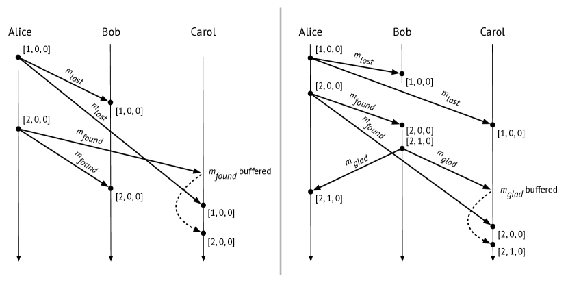
Figure 3. The executions from Figure 1, annotated with vector clocks used by the causal broadcast protocol. On the left, Carol buffers $m_{\mathit{found}}$ until she has delivered $m_{\mathit{lost}}$. On the right, Carol buffers $m_{\mathit{glad}}$ until she has delivered $m_{\mathit{found}}$.

2.2.3. Example Executions of the Causal Broadcast Protocol

To illustrate how the protocol works, Figure 3 shows the two problematic executions we saw previously in Figure 1, but now with the causal broadcast protocol in place to prevent violations of causal delivery. Each process keeps a vector clock with three entries corresponding to Alice, Bob, and Carol respectively. Suppose that $m_{\mathit{lost}}$ is Alice’s “I lost my wallet…” message, $m_{\mathit{found}}$ is Alice’s “Found it!” message, and $m_{\mathit{glad}}$ is Bob’s “Glad to hear it!” message.

In Figure 3 (left), Bob receives Alice’s messages in the order she broadcasted them, and so he can deliver them immediately. For example, when Bob receives $m_{\mathit{lost}}$, his own vector clock is [0,0,0], and the vector clock on the message is [1,0,0]. The message is deliverable at Bob’s process because it is one greater than Bob’s own vector clock in the sender’s (Alice’s) position, and less than or equal to Bob’s vector clock in the other positions, so Bob delivers it immediately after receiving it. Carol, on the other hand, receives $m_{\mathit{found}}$ first. This message has a vector clock of [2,0,0], so it is not immediately deliverable at Carol’s process because Carol’s vector clock is [0,0,0], and so the entry of 2 at the sender’s index is too large, indicating that the message is “from the future” and needs to be buffered in Carol’s delay queue for later delivery, after Carol delivers $m_{\mathit{lost}}$.

In Figure 3 (right), Bob delivers two messages from Alice and then broadcasts $m_{\mathit{glad}}$. $m_{\mathit{glad}}$ has a vector clock of [2,1,0], indicating that it has two messages sent by Alice in its causal history. When Carol receives $m_{\mathit{glad}}$, her own vector clock is only [1,0,0], indicating that she has only delivered one of those messages from Alice so far, so Carol must buffer $m_{\mathit{glad}}$ in her delay queue until she receives and delivers $m_{\mathit{found}}$, the missing message from Alice, increasing her own vector clock to [2,0,0]. Now $m_{\mathit{glad}}$ is deliverable at Carol’s process, and Carol can deliver it, increasing her own vector clock to [2,1,0].

2.3. Verification Task

Thanks to the relationship between the happens-before ordering and the vector clock ordering expressed by Equation 1, we can reduce the problem of determining that a distributed execution observes causal delivery to a condition that is locally checkable at each process. We call this condition local causal delivery:

Definition 0 (Local causal delivery).

A process $p$ observes local causal delivery if, for all messages $m_{1}$ and $m_{2}$ such that $\mathit{deliver}_{p}(m_{1})$ and $\mathit{deliver}_{p}(m_{2})$ are in $h_{p}$,

$\mathit{VC}(m_{1})<_{vc}\mathit{VC}(m_{2})\implies\mathit{deliver}_{p}(m_{1})\rightarrow_{p}\mathit{deliver}_{p}(m_{2})$.

The heart of our verification task will be to prove that our implementation of the causal broadcast protocol of Section 2.2 ensures that processes that run the protocol observe local causal delivery. From there, given Equation 1, we can prove that executions produced by a distributed system of processes that run the causal broadcast protocol observe global causal delivery:

Theorem 5 (Global Correctness of Causal Broadcast Protocol).

An execution in which all processes run the causal broadcast protocol observes causal delivery.

In the following sections, we show how we use Liquid Haskell to implement the causal broadcast protocol, to make the statement of Theorem 5 precise, and to prove Theorem 5. After presenting the implementation in Section 3, in Section 4 we develop the machinery necessary to express Definitions 2 and 4 and Theorem 5 as refinement types.

3. Implementation

In this section, we describe our implementation of Birman et al.’s causal broadcast protocol as a Liquid Haskell library. Section 3.1 describes the types we use to implement our system model and vector clock operations, and in Section 3.2 we give a brief overview of refinement types and Liquid Haskell before diving into our implementation of the protocol itself in Section 3.3. Finally, Section 3.4 discusses how a user application would use our library.

3.1. System Model and Vector Clocks

We begin by defining Haskell types to implement our system model and vector clock operations. Process identifiers are natural numbers and double as indexes into vector clocks, which are represented by a list of natural numbers. Messages have type M r, where the r parameter is the application-defined type of the raw message content (e.g., a JSON-formatted string).

⬇

type PID = Nat

type VC = [Nat]

data M r = M { mVC::VC, mSender::PID, mRaw::r }

A message has three fields: mVC and mSender are respectively the metadata that capture when the message was sent (as a VC) and who sent it (as a PID), and mRaw contains the raw message content.

An event can be either a Broadcast (to the network) or a Deliver (to the local user application for processing), and a process history H is a list of events.

⬇

data Event r = Broadcast (M r) | Deliver PID (M r)

type H r = [Event r]

To implement the vector clock protocol of Section 2.2.1, we need some standard vector clock operations, with the below interface:

⬇

vcEmpty :: Nat $\rightarrow$ VC

vcTick :: VC $\rightarrow$ PID $\rightarrow$ VC

vcCombine :: VC $\rightarrow$ VC $\rightarrow$ VC

vcLessEqual :: VC $\rightarrow$ VC $\rightarrow$ Bool

vcLess :: VC $\rightarrow$ VC $\rightarrow$ Bool

vcEmpty initializes a vector clock of a given size with zeroes, vcTick increments a vector clock at a given index, vcCombine computes the pointwise maximum of two vector clocks, and vcLessEqual and vcLess implement the vector clock ordering described in Section 2.2.1. As we will see in the following sections, our causal broadcast implementation uses vcTick and vcCombine when broadcasting and delivering messages, respectively. The prose definitions of all these operations translate directly into idiomatic Haskell; for example, the implementation of vcCombine is zipWith max.

3.2. Brief Background: Refinement Types and Liquid Haskell

Traditionally, refinement types (Rushby et al., 1998; Xi and Pfenning, 1998) have let programmers specify types augmented with logical predicates, called refinement predicates, that restrict the set of values that can inhabit a type. For example, in Liquid Haskell one could give vcCombine the following signature:

⬇

vcCombine :: v:VC $\rightarrow$ {v’ :VC | len v’ == len v}

$\rightarrow$ {v’’:VC | len v’’ == len v}

The refinement on v’ expresses the precondition that v and v’ will have the same length, and the return type expresses the postcondition that the returned vector clock will have the same length as the argument vector clocks. Liquid Haskell automatically proves that such postconditions hold by generating verification conditions that are checked at compile time by the underlying SMT solver (by default, Z3 (de Moura and Bjørner, 2008)). If the solver cannot ensure that the verification conditions are valid, typechecking fails. In our actual implementation, additional Liquid Haskell refinements on VC and PID — elided in this paper for readability — ensure that all functions are called with compatible vector clocks (having the same length) and PIDs (natural numbers smaller than the length of a vector clock).

Aside from preconditions and postconditions of individual functions, though, Liquid Haskell makes it possible to verify extrinsic properties that relate two functions, or calls to the same function applied to different inputs. As an example, here is a Liquid Haskell proof that vcCombine is commutative:

⬇

type Comm a A

= x:a $\rightarrow$ y:a $\rightarrow$ {_:Proof | A x y == A y x}

vcCombineComm :: n:Nat $\rightarrow$ Comm n {vcCombine}

vcCombineComm _n [] [] = ()

vcCombineComm n (_x:xs) (_y:ys) =

vcCombineComm (n - 1) xs ys

Here, vcCombineComm is a Haskell function that returns a value of Proof type (a type alias for (), Haskell’s unit type), refined by the predicate vcCombine x y == vcCombine y x. The proof is by induction on the structure of vector clocks. The base case, in which both x and y are empty lists, is automatic for the SMT solver, so the body of the base case need not say anything but (). The inductive case has a recursive call to vcCombineComm. We use a similar approach to prove that vcCombine is associative, idempotent, and inflationary, and that vcLess is a strict partial order. In general, programmers can specify arbitrary extrinsic properties in refinement types, including properties that refer to arbitrary Haskell functions via the notion of reflection (Vazou et al., 2017). The programmer can then prove those extrinsic properties by writing Haskell programs that inhabit those refinement types, using Liquid Haskell’s provided proof combinators — with the help of the underlying SMT solver to simplify the construction of these proofs-as-programs (Vazou et al., 2018, 2017).

Liquid Haskell thus occupies a position at the intersection of SMT-based program verifiers such as Dafny (Leino, 2010), and theorem provers that leverage the Curry-Howard correspondence such as Coq (Bertot and Castéran, 2004) and Agda (Norell, 2009). A Liquid Haskell program can consist of both application code like vcCombine (which runs at execution time, as usual) and verification code like vcCombineComm (which is never run, but merely typechecked), but, pleasantly, both are just Haskell programs, albeit annotated with refinement types. Since Liquid Haskell is based on Haskell, programmers can gradually port Haskell programs to Liquid Haskell, adding richer specifications to code as they go. For instance, a programmer might begin with an implementation of vcCombine with the type VC $\rightarrow$ VC $\rightarrow$ VC, later refine it to the more specific refinement type above, even later prove vcCombineComm, and still later use the proof returned by vcCombineComm as a premise to prove another, more interesting property.

3.3. Causal Broadcast Protocol Implementation

We express the causal broadcast protocol of Section 2.2 as a state transition system.

3.3.1. Process Type

The state data structure P r represents a process and is parameterized by the type of raw content, r:

⬇

data P r = P { pVC::VC, pID::PID, pDQ::[M r]

, pHist::{ h:H r | histVC h == pVC }}

The fields of P include the local vector clock pVC, the local process identifier pID, a delay queue of received but not-yet-delivered messages pDQ, and (importantly for our verification task) the process history pHist. We provide a pEmpty :: Nat $\rightarrow$ PID $\rightarrow$ P r function that initializes a process with a vector clock of the given length containing zeroes, the given process identifier, and an empty delay queue and empty process history.

The type of the process history pHist deserves further discussion, as it is our first use of a Liquid Haskell feature called datatype refinements. The datatype refinement on the pHist field says that it contains a history h of the type H r defined in the previous section, but with an additional constraint histVC h == pVC. This constraint expresses the intuition that the vector clock pVC and the history h “agree” with each other: for any process p starting with a pVC containing all zeros and an empty pHist, each addition of a Deliver (pID p) m event to the history for some message m must coincide with an update to pVC p of the form vcCombine (mVC m) (pVC p). Accordingly, histVC h is defined as the supremum of vector clocks on Deliver events in h. We extrinsically prove in Liquid Haskell that this pVC-pHist agreement property is true for the empty process and preserved by each transition in our state transition system. We next describe these transition functions.

3.3.2. State Transitions

The transition functions are receive, deliver, and broadcast, with the following interface:

⬇

receive :: M r $\rightarrow$ P r $\rightarrow$ P r

deliver :: P r $\rightarrow$ Maybe (M r, P r)

broadcast :: r $\rightarrow$ P r $\rightarrow$ (M r, P r)

The receive function adds a message from the network to the delay queue, the deliver function pops a deliverable message (if any) from the delay queue, and the broadcast function prepares raw content of type r for network transport by wrapping it in a message. Of these transition functions, only deliver and broadcast are particularly interesting from the perspective of our verification effort, since receive only adds messages to the delay queue and cannot affect whether causal delivery is violated. We next discuss the implementation of deliver and broadcast, respectively.

⬇

deliver :: P r $\rightarrow$ Maybe (M r, P r)

deliver p =

case dequeue (pVC p) (pDQ p) of

Nothing $\rightarrow$ Nothing

Just (m, pDQ’) $\rightarrow$

Just (m, p{ pVC = vcCombine (mVC m) (pVC p)

, pDQ = pDQ’

, pHist =

Deliver (pID p) m : pHist p })

dequeue :: VC $\rightarrow$ DQ r $\rightarrow$ Maybe (M r, DQ r)

dequeue _now [] = Nothing

dequeue now (x:xs)

| deliverable x now = Just (x, xs)

| otherwise = case dequeue now xs of

-- Skip past x.

Nothing $\rightarrow$ Nothing

Just (m, xs’) $\rightarrow$ Just (m, x:xs’)

deliverable :: M r $\rightarrow$ VC $\rightarrow$ Bool

deliverable m p_vc = let n = length p_vc in

and (zipWith3 (deliverableHelper (mSender m))

(finAsc n) (mVC m) p_vc)

deliverableHelper

:: PID $\rightarrow$ PID $\rightarrow$ Clock $\rightarrow$ Clock $\rightarrow$ Bool

deliverableHelper m_id k m_vc_k p_vc_k

| k == m_id = m_vc_k == p_vc_k + 1

| otherwise = m_vc_k <= p_vc_k

finAsc :: n:Nat $\rightarrow$

{ xs:[{x:Nat | x < n}]<{\a b $\rightarrow$ a < b}>

| len xs == n }

Figure 4. Implementation of deliver and its helpers.

3.3.3. Deliver

Figure 4 shows the implementation of deliver, as well as its constituents dequeue, deliverable, and deliverableHelper. At a high level, deliver calls dequeue on a process’s delay queue and then performs bookkeeping: If dequeue popped a deliverable message, then deliver returns that message and updates the process with a new vector clock according to the vector clock protocol, the new delay queue returned by dequeue, and a new process history which records the delivery of the message. The dequeue function plays its part by removing and returning the first deliverable message found in the delay queue.

The deliverable predicate implements the deliverability condition of Definition 3 to check whether a message m is deliverable at time p_vc. It works by calling deliverableHelper (mSender m) on each offset in the message vector clock mVC m and process vector clock p_vc, and returning the conjunction of those results. The function finAsc n provides those offsets in ascending order, and, combined with zipWith, lets us implement the subtle deliverability condition of Definition 3 in deliverableHelper, almost exactly as Definition 3 is written (except that our vector clocks are zero-indexed). We omit the implementation of finAsc from Figure 4 for brevity, but its refinement type guarantees that it returns an ascending list of length n containing Nats less than n, using Liquid Haskell’s abstract refinements feature (Vazou et al., 2013).

3.3.4. Broadcast

⬇

broadcast :: r $\rightarrow$ P r $\rightarrow$ (M r, P r)

broadcast raw p =

let m = M { mVC = vcTick (pVC p) (pID p)

, mSender = pID p

, mRaw = raw }

p’ = p { pDQ = m : pDQ p

, pHist = Broadcast m : pHist p }

Just tup = deliver p’

in tup

Figure 5. Implementation of broadcast. We prove that deliver p’ is a Just value using an extrinsic proof.

Figure 5 shows the implementation of the broadcast function. First, broadcast constructs a message m for the value raw by incrementing the pID p index of its own vector clock pVC p, and attaching that pID p to m as mSender. Next, broadcast constructs an intermediate process value p’ containing m at the head of the delay queue and a new process history recording the broadcast event for this message. Last, broadcast delegates to deliver to deliver m at its own sender, p’. As we will see in Section 4, implementing broadcast in terms of deliver simplifies proving properties about our implementation, because proofs about broadcast can often delegate to existing proofs about deliver.

Although deliver’s return type is Maybe (M r, P r), the deliver p’ call in broadcast is guaranteed by Liquid Haskell to evaluate to a Just value containing the next process and the message to be broadcast. We prove this property using an extrinsic proof, not shown here. The intuition is that messages a process sends to itself are always immediately deliverable, because when a process increments its own index in the vector clock that it places in a message, the message immediately becomes deliverable at that process.

3.4. Example Application Architecture

The receive, deliver, and broadcast functions are the interface made available to user applications of our causal broadcast library. When deliver returns a message, the user application must process it immediately. The user application must also immediately put the message returned by broadcast on the network and also process the message locally. This design implies that user applications should not update their own state directly when communication is in order, but rather, generate a message and then update their state in response to its delivery.

Figure 6 shows an example architecture of an application using our causal broadcast library. A collection of (potentially geo-distributed) peer nodes, which we call the causal broadcast cluster, each run the causal broadcast protocol along with their user application code (for instance, a key-value store or a group chat application). Clients of the application communicate their requests to the nodes; one or more clients may communicate with each node. The application instance on a node generates messages, broadcasts them to other nodes, and delivers messages received from other nodes. Later on, in Section 5, we will see a case study of an application with this architecture.

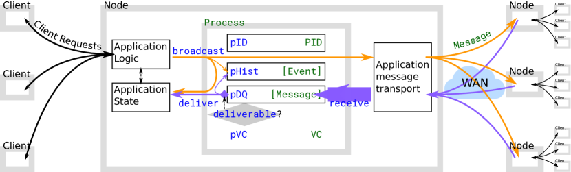
Figure 6. Example architecture for a distributed application using our causal broadcast library. The mnemonic standins Process, Event, and Message refer to the types P r, Event r, and M r defined in our implementation. An application node using this architecture participates in the causal broadcast protocol using a single process data structure and the functions receive, broadcast, and deliver to safely manage message-passing state. Clients make requests to a node, possibly updating application state, and the node may generate messages to replicate updates or perform other tasks.

4. Verification

In this section we mechanize causal delivery and local causal delivery (Definitions 4 and 2) for our implementation of the causal broadcast protocol, and we describe the highlights of our Liquid Haskell proof development, culminating in a mechanized proof of Theorem 5. In Section 4.1 we show how we express local causal delivery (abbreviated “LCD” henceforth) as a refinement type in Liquid Haskell, and in Section 4.2 we show that each of the receive, deliver, and broadcast transitions of Section 3.3 results in a process that observes LCD. We then leverage this fact to prove Theorem 5 in Section 4.3. Finally, in Section 4.4 we briefly discuss the liveness of our implementation.

4.1. Local Causal Delivery as a Refinement Type

As we saw in Section 3.3.1, a process tracks the history of events that have occurred on it so far, including message broadcasts and deliveries. We can examine a process’s history and see whether the process has been delivering messages in an order consistent with the messages’ vector clock ordering. Therefore, we can express local causal delivery (Definition 4) as a refinement type as follows:

⬇

type LocalCausalDelivery r ID HIST

= {m1 : M r | elem (Deliver ID m1) HIST }

$\rightarrow$ {m2 : M r | elem (Deliver ID m2) HIST

&& vcLess (mVC m1) (mVC m2) }

$\rightarrow$ { _:Proof | processOrder HIST

(Deliver ID m1) (Deliver ID m2) }

The type alias LocalCausalDelivery r ID HIST fixes a process identifier ID and a process history HIST. It is the type of a function that given messages m1 and m2, both of which have already been delivered in the specified process history and for which the vector clock of m1 is less than that of m2, produces a proof that the delivery event of m1 precedes the delivery event of m2 in the process history. The vcLess function is part of the vector clock interface described in Section 3.1, and the predicate processOrder h e e’ returns True if event e is present in the list of events that precede event e’ in a process history h.

The LocalCausalDelivery type captures what it means for a given process to observe LCD: it says that if we consider any two messages that are in the process’s history, and those messages’ vector clocks have an order, then there is evidence – in this case, in the form of an affirmative answer from an SMT solver – that those messages appear in the process history in their vector clock order, rather than the other way around. Our next step will be to show that this LCD property actually holds for processes running our implementation of the causal broadcast protocol.

4.2. Local Causal Delivery Preservation

Recall the state transition system consisting of the process type P r and the functions receive, deliver, and broadcast discussed in Section 3.3. We need to prove (1) that a process observes LCD in its initial, empty state returned by pEmpty, and (2) that whenever a process satisfying LCD transitions to a new state via any sequence of steps of the receive, deliver, or broadcast transition functions, the resulting process state still observes LCD. A proof that the empty process observes LCD as defined in Section 4.1 is trivially discharged by Liquid Haskell, so we turn our attention to proving that each of the state transitions preserves LCD. Most of the action of our proof development happens in handling deliver steps, as we will see below in Section 4.2.1.

To use the LocalCausalDelivery type alias with the process type, P r, we need a small adapter to extract the pID and pHist fields.

⬇

type LCD r PROC =

LocalCausalDelivery r {pID PROC} {pHist PROC}

To encode the inputs to each of the causal broadcast protocol transition functions, we define a sum type over the arguments, Op r. Each function takes a P r input and additional arguments corresponding to one of the Op r constructors.

⬇

data Op r = OpReceive (M r)

| OpDeliver

| OpBroadcast r

To apply those transition functions to a process value, we define step. It branches on the constructor of Op r, calls a transition function discussed in Section 3.3, extracts the next process value, and throws away information unneeded for the proof.

⬇

step :: Op r $\rightarrow$ P r $\rightarrow$ P r

step (OpReceive m) p = receive m p

step (OpBroadcast r) p = case broadcast r p of

(_, p’) $\rightarrow$ p’

step (OpDeliver ) p = case deliver p of

Just (_, p’) $\rightarrow$ p’

Nothing $\rightarrow$ p

Next, we prove a stepLCD lemma, which states that for a given operation op and process p, if LCD holds for p, then it still holds after applying op to p using step:

⬇

stepLCD :: op : Op r

$\rightarrow$ p : P r

$\rightarrow$ LCD r {p}

$\rightarrow$ LCD r {step op p}

The proof of stepLCD branches on the constructors for op, followed by delegation to lemmas about each of the transition functions.

⬇

stepLCD op p pLCD =

case op ? step op p of

OpBroadcast r $\rightarrow$ broadcastLCDpres r p pLCD

OpReceive m $\rightarrow$ receiveLCDpres m p pLCD

OpDeliver $\rightarrow$ deliverLCDpres p pLCD

By far the most involved of these three lemmas is deliverLCDpres, the one that deals with deliver steps. Proving broadcastLCDpres is straightforward because calling broadcast only adds a Broadcast event to the process history (and then calls deliver), and so if a process observes LCD before calling broadcast, then it is easy to show that it still does after adding the event (and for calling deliver to deliver the message locally, we can delegate to deliverLCDpres). Proving receiveLCDpres is even more straightforward because calling receive does not modify the process history, and so if a process observes LCD before calling receive, it is easy to show that it still does afterward. We therefore omit discussion of receiveLCDpres and broadcastLCDpres and focus on the proof of deliverLCDpres in the next section.

4.2.1. Deliver Transition Preservation Lemma

The deliverLCDpres lemma states that a process’s observation of LCD is preserved through calls to the deliver function. The proof begins by deconstructing the two cases of dequeue, echoing the definition of deliver (Figure 4). In the case that dequeue returns Nothing, so does its caller deliver, and the process state is unchanged. This line of reasoning is automatically carried out by Liquid Haskell without needing to be explicitly written in the proof. As a result, we can use the input evidence that the original process observes LCD to complete the case.

More interesting is the case in which dequeue returns a message m that has been deemed deliverable. We need to show that in an updated process state p’ in which m has been delivered, the process still observes LCD. Recalling the definition of LocalCausalDelivery from Section 4.1, we need to show that for all messages m1 and m2 where the vector clock of m1 is less than that of m2, m1’s delivery event occurs before m2’s delivery event in p’’s process history. There are three cases to consider:

• Case m == m1. When m is equal to m1, it is the most recently delivered message on p’, but since vcLess (mVC m1) (mVC m2), this would be a causal violation, and so we show this case is impossible. Recall that since m was deliverable on the original process p, deliverable m (pVC p) is True, which implies a relationship between mVC m and pVC p: the mSender m offset in mVC m is exactly one greater than that of pVC p, and all other offsets of mVC m are less than or equal to that of pVC p. Additionally, vcLessEqual (mVC m1) (mVC m2) by vcLess, and vcLessEqual (mVC m2) (histVC p) because the delivery of m2 is in pHist p and because vcCombine is inflationary, and histVC p == pVC p by the data refinement on processes. Finally, since vcLessEqual is transitive, we can combine these facts to conclude that vcLessEqual (mVC m1) (pVC p), which contradicts the relationship implied by deliverable m (pVC p).

• Case m == m2. When m is equal to m2, it is the most recently delivered message on p’. Let e1 be the delivery event for m1 with the definition Deliver (pID p’) m1 and similarly let e2 be the delivery event for the equivalent messages m2 and m. Since pHist p’ is e2:pHist p, and e1 is known to already be in pHist p, we can conclude that e1 precedes e2 in p’’s history, and so processOrder (pHist p’) e1 e2, as required by LCD.

• Case m /= m1 && m /= m2. Finally, when m is a new message distinct from both m1 and m2, we show that the addition of a deliver event for m to pHist p does not change the delivery ordering of m1 and m2. That is, with event e1 for delivery of m1, e2 for m2, and e3 for m, since pHist p’ is e3:pHist p, and since e1 and e2 were in pHist p (and both are still in pHist p’), we can conclude that orderings about elements in pHist p are unchanged in pHist p’.

With these pieces in place, we can conclude that a LCD-observing process continues to observe LCD after any call to deliver.

Description	LOC
Implementation without refinements	236
Implementation-supporting proofs and refinements	448
List lemmas, extra proof combinators, shims	161
Proofs about relations (Section 3.1)	217
Model for preservation of LCD (Section 4.1)	27
LCD preservation (LABEL:{subsec_verif_pres_plcd})	51
LCD preservation, broadcast case	64
LCD preservation, receive case	44
LCD preservation, deliver case (Section 4.2.1)	273
Model for preservation of CD (Section 4.3)	130
CD preservation	138
CD preservation via LCD	139

Table 1. Lines of code used in our implementation and proof development. The LOC count includes Liquid Haskell definitions, theorems, proofs, and other annotations.

4.3. Global Causal Delivery Preservation

The lcdStep property we proved in the previous section says that running the causal broadcast protocol for one step on a given process preserves local causal delivery for that process. However, Theorem 5 pertains to entire executions as opposed to individual processes. To complete the proof, then, we must define an additional global state transition system, where states represent executions, and a step nondeterministically picks any process in an execution and runs the causal broadcast protocol for one (local) step on that process. Unlike the local state transition system, which is actually what is used at run time to execute the causal broadcast protocol, our global states and global steps are for verification purposes only.

We define a global execution state as a mapping from PIDs to P r process states. We can then express (global) causal delivery (Definition 2) as a refinement type, as follows:

⬇

type CausalDelivery r X

= pid : PID

$\rightarrow$ {m1 : M r | elem (Deliver pid m1)

(pHist (X pid)) }

$\rightarrow$ {m2 : M r | elem (Deliver pid m2)

(pHist (X pid))

&& happensBefore X

(Broadcast m1)

(Broadcast m2) }

$\rightarrow$ {_: Proof | processOrder (pHist (X pid))

(Deliver pid m1)

(Deliver pid m2) }

The CausalDelivery type is reminiscent of the LocalCausalDelivery type that we saw in Section 4.1, but instead of referring to one particular process, it refers to an entire execution, X. CausalDelivery r X says that for any process in X, messages are delivered in causal order on that process. Another key difference is that instead of using vcLess, CausalDelivery uses a happensBefore predicate, which takes an execution argument and two events. This is as it should be; the definition of causal delivery should be agnostic to the mechanism used by our particular protocol. However, our lcdStep lemma only establishes that messages on a process are delivered in an order consistent with their vector-clock ordering, not the happens-before ordering. To bridge this gap and get from local causal delivery to global causal delivery, we must leverage Equation 1’s correspondence between vector clocks and happens-before, which we express as a pair of axioms in Liquid Haskell, one for each direction of the correspondence.

We can now prove that a single global execution step preserves causal delivery. The xStepCD lemma states that if we have a causal-delivery-observing execution x, if we pick out any given process (identified by pid) from that execution and run any given operation op on that process, then the resulting execution will also observe causal delivery.

⬇

xStepCD :: op: Op r

$\rightarrow$ x: Execution

$\rightarrow$ pid: PID

$\rightarrow$ CausalDelivery r x

$\rightarrow$ CausalDelivery r {xStep op pid x}

The proof of xStepCD proceeds in three stages:

1. Global to local. First, we show that if the original execution observes causal delivery, then every process in it observes local causal delivery. For this, we use the reflection direction of the vector-clock/happens-before correspondence, which says that messages with a given vector clock ordering were broadcast in the corresponding happens-before order.

2. Local step. Next, we show that if any process in an execution takes a local step, then every process in the execution will still observe local causal delivery. This is easy to show using our lcdStep lemma.

3. Local to global. Finally, we show that if every process in an execution observes local causal delivery, then the entire execution observes causal delivery. For this, we use the preservation direction of the vector-clock/happens-before correspondence, which says that messages broadcast in a given happens-before order have the corresponding vector clock order.

Since the vector-clock/happens-before correspondence lets us reason in a process-local fashion, instead of having to reason about events spread across a global execution using happens-before, we enjoy a sort of “local reasoning for free” without the need for a more heavyweight proof technique such as separation logic. With the proof of xStepCD complete, all that remains to prove Theorem 5 is to extrapolate from global executions that take one step to those that take any number of steps, which is straightforward to do in Liquid Haskell by induction on the number of steps. Since an empty global execution observes causal delivery, we can conclude that any global execution where all processes are running our protocol observes causal delivery, completing the proof of Theorem 5.

Table 1 summarizes the size of each component of our proof development in terms of lines of Liquid Haskell code, and Figure 7 gives a visual overview of the important components of the proof: the xStepCD property and its proof in three stages outlined above; the stepLCD property and its reliance on lemmas for broadcast, receive, and deliver, and our use of the two directions of the vector-clock/happens-before correspondence. In all, our proof development weighs in at 1692 lines of code for 236 lines of implementation code.

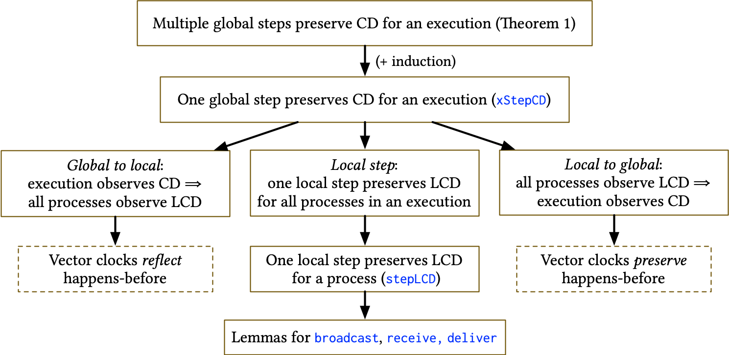
Figure 7. A high-level overview of the key components of our proof development. Arrows indicate dependencies, solid boxes indicate theorems and lemmas, and dashed boxes indicate axioms.

4.4. Discussion: Liveness

A useful implementation is not only safe, but live, which in our case would mean that messages will not languish forever in the delay queue. As mentioned in Section 2.1, for our safety result we need not make any assumption of reliable message receipt, since we do not have to worry about the delivery order of messages that are never received. A proof of liveness, though, would need to rest on the assumption of a reliable message transport layer, that is, one in which sent messages are eventually received — albeit in arbitrary order and with arbitrarily long latency. Otherwise, a message could be stuck forever in the delay queue if a message that causally precedes it is lost, because it would never become deliverable. Proofs of liveness properties are considered “much harder” (Hawblitzel et al., 2015) than proofs of safety properties. While we do not offer any mechanized liveness proof, in the following section we argue informally for the liveness of our implementation under the reliable message reception assumption.

5. Case study

In this section we describe a key-value store (KVS) application implemented in the architectural pattern depicted by Figure 6 and using our causal broadcast library from Section 3. The KVS is an in-memory replicated data store consisting of message-passing nodes, each of which simultaneously serves client requests via HTTP. Section 5.1 covers the implementation of the KVS and demonstrates that it is not difficult to integrate our causal broadcast protocol with an application to obtain the benefits of causal broadcast. In particular, causal broadcast can be used to ensure causal consistency of replicated data (Ahamad et al., 1995; Lloyd et al., 2011). In Section 5.2 we describe how we deployed the KVS to a cluster of geo-distributed nodes and evaluated its performance.

5.1. Design and Implementation

We implemented the KVS using several commonly used Haskell libraries, such as servant (Mestanogullari et al., 2015) to express HTTP endpoints concisely as types, stm to express multithreaded access to state, ekg to gather runtime statistics, and aeson to provide JSON (de)serialization. Clients may request to PUT a value at a key, DELETE a key-value pair specified by key, or GET the value corresponding to a specified key. Servers broadcast by directly POSTing messages to each other. Nodes receiving PUT or DELETE requests from their local clients call broadcast to prepare a message to be immediately applied locally and broadcast to other nodes. When a node makes a POST request, the endpoint calls receive to inject the message into the node’s delay queue. Changes to the delay queue wake a background thread which calls deliver, possibly removing a message from the delay queue and applying it to the process state. Since messages received via the POST endpoint are from other nodes, deliver will return Nothing in cases where the causal dependencies of the message are not satisfied. Therefore all nodes (and hence all clients of those nodes) observe the effects of causally-related KvCommands in the same (causal) order.

5.2. Deployment and Evaluation

We deployed an eight-node KVS causal broadcast cluster, globally distributed across AWS regions (two nodes in us-west-1 (N. California), one in us-west-2 (Oregon), two in us-east-1 (N. Virginia), one in ap-northeast-1 (Tokyo), and two in eu-central-1 (Frankfurt)), and 24 client nodes with three clients assigned to each KVS node. All the nodes were AWS EC2 t3.micro instances with 2 vCPUs at 2.5 GHz and 1 GiB of memory. The 50th-percentile inter-region ping latencies vary from about 20ms between us-west-1 and us-west-2 to about 225ms between ap-northeast-1 and eu-central-1. Each of the eight nodes in the cluster ran an instance of our KVS application compiled with GHC 8.10.7.

We conducted a simple experiment in which each of the 24 clients made 10,000 curl requests at 20 requests per second to their assigned KVS replica in the same region (for a total of 240,000 client requests), uniformly distributed over GET, PUT, and DELETE requests. For PUT requests, we used randomly generated JSON data for values, and ensured that there were key collisions, requiring resolution by causal order, by drawing keys from among the lowercase ASCII characters.

Two-thirds (160,000) of the 240,000 requests generated by clients were PUT and DELETE requests. Each resulted in a broadcast from the client’s assigned KVS replica to the seven other nodes in the cluster, generating 160,000 $\times$ 7 = 1,120,000 unicast messages among the eight KVS nodes. To alleviate this message amplification and maintain throughput, we sent multiple unicast messages in each request; typically, two or three messages were sent at a time. The KVS replicas handled all requests and delivered all messages in the time it took for clients to send them (10 minutes) with a load average of 0.10, indicating that the cluster was not CPU-bound and that no messages got stuck indefinitely in delay queues. As a static verification approach, Liquid Haskell itself imposes no running time overhead compared to vanilla Haskell, and no Liquid Haskell annotations were required in the KVS application code.

We recorded the length of the delay queue after each message delivery and maintained an average. Over all nodes, the average length of the delay queue after a delivery came to 7.2 delayed messages. From prior experiments with a different mix of KVS nodes and clients, we observe that more nodes in the causal broadcast cluster results in increased likelihood of messages being received out of causal order, motivating the need for causal broadcast.

6. Related Work

Machine-checked correctness proofs of executable distributed protocol implementations.

Much work on distributed systems verification has focused on specifying and verifying properties of models using tools such as TLA+ (Lamport, 2002), rather than of executable implementations. Here, our focus is on mechanized verification of executable distributed protocol implementations; lacking space for a comprehensive account of the literature, we mention a few highlights.

Verdi (Wilcox et al., 2015) is a Coq framework for implementing distributed systems; verified executable OCaml implementations can be extracted from Coq. IronFleet (Hawblitzel et al., 2015) uses the Dafny verification language, which compiles both to verification conditions checked by an SMT solver and to executable code. Both Verdi and IronFleet have been used to verify safety properties (in particular, linearizability) of distributed consensus protocol implementations (Raft and Multi-Paxos, respectively) and of strongly-consistent key-value store implementations, and IronFleet additionally considers liveness properties. The ShadowDB project (Schiper et al., 2014) uses a language called EventML that compiles both to a logical specification and to executable code that is automatically guaranteed to satisfy the specification, and correctness properties of the logical specification can then be proved using the Nuprl proof assistant. Schiper et al. (2014) used this workflow to verify the correctness of a Paxos-based atomic broadcast protocol. None of Wilcox et al., Hawblitzel et al., or Schiper et al. looked at causal broadcast or causal message ordering in particular.

Lesani et al. (2016) present a technique and Coq-based framework for mechanically verifying the causal consistency of distributed key-value store (KVS) implementations, with executable OCaml KVSes extracted from Coq. Lesani et al.’s verification approach effectively bakes a notion of causal message delivery into an abstract causal operational semantics that specifies how a causally consistent KVS should behave. In more recent work, Gondelman et al. (2021) use the Coq-based Aneris distributed separation logic framework (Krogh-Jespersen et al., 2020) — itself built on top of the Iris separation logic framework (Jung et al., 2018) — to specify and verify the causal consistency of a distributed KVS and further verify the correctness of a session manager library implemented on top of the KVS. These implementations are written in AnerisLang, a domain-specific language intended to be used with the Aneris framework for implementing distributed systems. Both Lesani et al.’s and Gondelman et al.’s work is specific to the KVS use case, whereas our verified causal broadcast implementation factors out causal message delivery into a separate layer, agnostic to the content of messages, that can be used as a standalone component in a variety of applications. Moreover, Liquid Haskell’s SMT automation simplifies our proof effort by comparison. Unlike Lesani et al. and Gondelman et al., we did not attempt to verify the causal consistency of our KVS. However, we hypothesize that building on an underlying verified causal messaging layer would simplify the KVS verification task by separating lower-level message delivery concerns from higher-level application semantics.

Causal broadcast for CRDT convergence.

Conflict-free replicated data types (CRDTs) (Shapiro et al., 2011b, a) are data structures designed for replication. Their operations must satisfy certain mathematical properties that can be leveraged to ensure strong convergence (Shapiro et al., 2011b), meaning that replicas are guaranteed to have equivalent state if they have received and applied the same unordered set of updates. While the simplest CRDTs ask little of the underlying messaging layer, many CRDTs implemented in the operation-based style rely on causal delivery to ensure that, for example, a message updating an element of a set will not be delivered before the message inserting that element.

Gomes et al. (2017) use the Isabelle/HOL proof assistant (Wenzel et al., 2008) to implement and verify the strong convergence of operation-based CRDTs under an assumption of causal delivery, modeled by the network axioms in their proof development. Our work is complementary to Gomes et al.’s: one could deploy their verified-convergent CRDTs atop our verified causal broadcast protocol to get an “end-to-end” convergence guarantee on top of a weaker network model that offers no causal delivery guarantee.

Liu et al. (2020) use Liquid Haskell to verify the convergence of operation-based CRDT implementations. Liu et al.’s CRDTs do not assume causal delivery, which complicates their implementation (and verification). In fact, Liu et al.’s verified two-phase map implementation includes a “pending buffer” for updates that arrived out of order, and a collection of data-structure-specific rules to determine which updates should be buffered. These mechanisms resemble the delay queue and the deliverable predicate, but are specific to application-level data structures and use an ad hoc delivery policy, rather than operating at the messaging layer and using the more general principle of causal delivery. We hypothesize that our library could lessen the need for such ad hoc mechanisms.

The most closely related work to this paper — and the only other mechanically verified causal broadcast implementation that we are aware of — was recently carried out by Nieto et al. (2022) as part of a larger proof development that verifies the correctness of a variety of CRDTs using the aforementioned Aneris separation logic framework. Nieto et al.’s proof development consists of a verified stack of components, at the base of which is a verified causal broadcast library, followed by a library of CRDT components, and finally CRDT implementations. To verify the causal broadcast library, Nieto et al. take a similar approach to Gondelman et al.’s aforementioned verified key-value store, but adapted to the more general setting of causal broadcast. Their approach thus supports our hypothesis that it is possible to simplify the verification of higher-level application properties, such as causal consistency of a key-value store or convergence of CRDTs, by decoupling them from lower-level message delivery properties, such as causal broadcast.

Compared to our work, Nieto et al.’s verification effort is more broadly scoped: most obviously, they tackle verification of clients of causal broadcast, in addition to the causal broadcast protocol itself. Additionally, their implementation is intended to be used on top of an unreliable transport protocol, UDP, and as such it includes mechanisms to ensure reliable message delivery (although their verification, like ours, is limited to safety properties only). We deploy and empirically evaluate the performance of our implementation, whereas Nieto et al. do not. Finally, our approach differs from Nieto et al.’s conceptually in that we frame the problem in terms of refinement types, whereas Nieto et al. take the separation-logic approach of defining logical resources and giving specifications about how those resources are used by their implementations. Our use of Liquid Haskell lets us take advantage of SMT automation where possible, using manual proofs only when needed. On the other hand, Nieto et al.’s use of standard separation logic mechanisms is a boon for modularity.

7. Conclusion

Causal message broadcast is a widely used building block of distributed applications, motivating the need for practically usable verified implementations. We use Liquid Haskell to give a novel encoding of causal message delivery as a refinement type. We then verify the safety of an executable causal broadcast library implemented in Haskell using a combination of manual theorem proving and SMT automation. Our verified-safe library can be used in real distributed systems, as we demonstrate with a case-study implementation and deployment of a distributed key-value store.

Acknowledgments

This material is based upon work supported by the National Science Foundation under Grant No. CCF-2145367. Any opinions, findings, and conclusions or recommendations expressed in this material are those of the author(s) and do not necessarily reflect the views of the National Science Foundation.

References

- (1)
- Acharya and Badrinath (1992) Arup Acharya and B.R. Badrinath. 1992. Recording distributed snapshots based on causal order of message delivery. Inform. Process. Lett. 44, 6 (1992), 317 – 321. https://doi.org/10.1016/0020-0190(92)90107-7
- Ahamad et al. (1995) Mustaque Ahamad, Gil Neiger, James E. Burns, Prince Kohli, and Phillip W. Hutto. 1995. Causal memory: definitions, implementation, and programming. Distributed Computing 9, 1 (1995), 37–49. https://doi.org/10.1007/BF01784241
- Alagar and Venkatesan (1994) Sridhar Alagar and S. Venkatesan. 1994. An optimal algorithm for distributed snapshots with causal message ordering. Inform. Process. Lett. 50, 6 (1994), 311 – 316. https://doi.org/10.1016/0020-0190(94)00055-7
- Bertot and Castéran (2004) Yves Bertot and Pierre Castéran. 2004. Interactive Theorem Proving and Program Development - Coq’Art: The Calculus of Inductive Constructions. Springer. https://doi.org/10.1007/978-3-662-07964-5
- Birman and Joseph (1987a) K. Birman and T. Joseph. 1987a. Exploiting Virtual Synchrony in Distributed Systems. SIGOPS Oper. Syst. Rev. 21, 5 (Nov. 1987), 123–138. https://doi.org/10.1145/37499.37515
- Birman et al. (1991) Kenneth Birman, André Schiper, and Pat Stephenson. 1991. Lightweight Causal and Atomic Group Multicast. ACM Trans. Comput. Syst. 9, 3 (Aug. 1991), 272–314. https://doi.org/10.1145/128738.128742
- Birman and Joseph (1987b) Kenneth P. Birman and Thomas A. Joseph. 1987b. Reliable Communication in the Presence of Failures. ACM Trans. Comput. Syst. 5, 1 (Jan. 1987), 47–76. https://doi.org/10.1145/7351.7478
- Bouajjani et al. (2017) Ahmed Bouajjani, Constantin Enea, Rachid Guerraoui, and Jad Hamza. 2017. On Verifying Causal Consistency. In Proceedings of the 44th ACM SIGPLAN Symposium on Principles of Programming Languages (Paris, France) (POPL 2017). Association for Computing Machinery, New York, NY, USA, 626–638. https://doi.org/10.1145/3009837.3009888
- de Moura and Bjørner (2008) Leonardo de Moura and Nikolaj Bjørner. 2008. Z3: An Efficient SMT Solver. In Tools and Algorithms for the Construction and Analysis of Systems, C. R. Ramakrishnan and Jakob Rehof (Eds.). Springer Berlin Heidelberg, Berlin, Heidelberg, 337–340.
- Fidge (1988) C. J. Fidge. 1988. Timestamps in message-passing systems that preserve the partial ordering. Proceedings of the 11th Australian Computer Science Conference 10, 1 (1988), 56–66.
- Gomes et al. (2017) Victor B. F. Gomes, Martin Kleppmann, Dominic P. Mulligan, and Alastair R. Beresford. 2017. Verifying Strong Eventual Consistency in Distributed Systems. Proc. ACM Program. Lang. 1, OOPSLA, Article 109 (Oct. 2017), 28 pages. https://doi.org/10.1145/3133933
- Gondelman et al. (2021) Léon Gondelman, Simon Oddershede Gregersen, Abel Nieto, Amin Timany, and Lars Birkedal. 2021. Distributed Causal Memory: Modular Specification and Verification in Higher-Order Distributed Separation Logic. Proc. ACM Program. Lang. 5, POPL, Article 42 (Jan. 2021), 29 pages. https://doi.org/10.1145/3434323
- Hawblitzel et al. (2015) Chris Hawblitzel, Jon Howell, Manos Kapritsos, Jacob R. Lorch, Bryan Parno, Michael L. Roberts, Srinath Setty, and Brian Zill. 2015. IronFleet: Proving Practical Distributed Systems Correct. In Proceedings of the 25th Symposium on Operating Systems Principles (Monterey, California) (SOSP ’15). Association for Computing Machinery, New York, NY, USA, 1–17. https://doi.org/10.1145/2815400.2815428
- Jung et al. (2018) Ralf Jung, Robbert Krebbers, Jacques-Henri Jourdan, Aleš Bizjak, Lars Birkedal, and Derek Dreyer. 2018. Iris from the ground up: A modular foundation for higher-order concurrent separation logic. Journal of Functional Programming 28 (2018), e20. https://doi.org/10.1017/S0956796818000151
- Krogh-Jespersen et al. (2020) Morten Krogh-Jespersen, Amin Timany, Marit Edna Ohlenbusch, Simon Oddershede Gregersen, and Lars Birkedal. 2020. Aneris: A Mechanised Logic for Modular Reasoning about Distributed Systems. In Programming Languages and Systems - 29th European Symposium on Programming, ESOP 2020, Held as Part of the European Joint Conferences on Theory and Practice of Software, ETAPS 2020, Dublin, Ireland, April 25-30, 2020, Proceedings. 336–365. https://doi.org/10.1007/978-3-030-44914-8_13
- Lamport (1978) Leslie Lamport. 1978. Time, Clocks, and the Ordering of Events in a Distributed System. Commun. ACM 21, 7 (July 1978), 558–565. https://doi.org/10.1145/359545.359563
- Lamport (2002) Leslie Lamport. 2002. Specifying Systems: The TLA+ Language and Tools for Hardware and Software Engineers. Addison-Wesley Longman Publishing Co., Inc., USA.
- Leino (2010) K. Rustan M. Leino. 2010. Dafny: An Automatic Program Verifier for Functional Correctness. In Proceedings of the 16th International Conference on Logic for Programming, Artificial Intelligence, and Reasoning (Dakar, Senegal) (LPAR’10). Springer-Verlag, Berlin, Heidelberg, 348–370.
- Lesani et al. (2016) Mohsen Lesani, Christian J. Bell, and Adam Chlipala. 2016. Chapar: Certified Causally Consistent Distributed Key-Value Stores. In Proceedings of the 43rd Annual ACM SIGPLAN-SIGACT Symposium on Principles of Programming Languages (St. Petersburg, FL, USA) (POPL ’16). Association for Computing Machinery, New York, NY, USA, 357–370. https://doi.org/10.1145/2837614.2837622
- Liu et al. (2020) Yiyun Liu, James Parker, Patrick Redmond, Lindsey Kuper, Michael Hicks, and Niki Vazou. 2020. Verifying Replicated Data Types with Typeclass Refinements in Liquid Haskell. Proc. ACM Program. Lang. 4, OOPSLA, Article 216 (Nov. 2020), 30 pages. https://doi.org/10.1145/3428284
- Lloyd et al. (2011) Wyatt Lloyd, Michael J. Freedman, Michael Kaminsky, and David G. Andersen. 2011. Don’t Settle for Eventual: Scalable Causal Consistency for Wide-Area Storage with COPS. In Proceedings of the Twenty-Third ACM Symposium on Operating Systems Principles (Cascais, Portugal) (SOSP ’11). Association for Computing Machinery, New York, NY, USA, 401–416. https://doi.org/10.1145/2043556.2043593
- Mahajan et al. (2011) P. Mahajan, L. Alvisi, and M. Dahlin. 2011. Consistency, Availability, Convergence. Technical Report TR-11-22. Computer Science Department, University of Texas at Austin.
- Mattern (1989) Friedemann Mattern. 1989. Virtual Time and Global States of Distributed Systems. In Parallel and Distributed Algorithms. North-Holland, 215–226.
- Mestanogullari et al. (2015) Alp Mestanogullari, Sönke Hahn, Julian K. Arni, and Andres Löh. 2015. Type-Level Web APIs with Servant: An Exercise in Domain-Specific Generic Programming. In Proceedings of the 11th ACM SIGPLAN Workshop on Generic Programming (Vancouver, BC, Canada) (WGP 2015). Association for Computing Machinery, New York, NY, USA, 1–12. https://doi.org/10.1145/2808098.2808099
- Nieto et al. (2022) Abel Nieto, Léon Gondelman, Alban Reynaud, Amin Timany, and Lars Birkedal. 2022. Modular Verification of Op-Based CRDTs in Separation Logic. Proc. ACM Program. Lang. 6, OOPSLA2, Article 188 (Oct. 2022), 29 pages. https://doi.org/10.1145/3563351
- Norell (2009) Ulf Norell. 2009. Dependently Typed Programming in Agda. Springer Berlin Heidelberg, Berlin, Heidelberg, 230–266. https://doi.org/10.1007/978-3-642-04652-0_5
- Postel (1981) Jon Postel. 1981. Transmission Control Protocol. STD 7. RFC Editor. http://www.rfc-editor.org/rfc/rfc793.txt
- Raynal et al. (1991) Michel Raynal, André Schiper, and Sam Toueg. 1991. The causal ordering abstraction and a simple way to implement it. Inform. Process. Lett. 39, 6 (1991), 343–350. https://doi.org/10.1016/0020-0190(91)90008-6
- Rushby et al. (1998) J. Rushby, S. Owre, and N. Shankar. 1998. Subtypes for specifications: predicate subtyping in PVS. IEEE Transactions on Software Engineering 24, 9 (1998), 709–720. https://doi.org/10.1109/32.713327
- Schiper et al. (1989) André Schiper, Jorge Eggli, and Alain Sandoz. 1989. A New Algorithm to Implement Causal Ordering. In Proceedings of the 3rd International Workshop on Distributed Algorithms. Springer-Verlag, Berlin, Heidelberg, 219–232.
- Schiper et al. (2014) N. Schiper, V. Rahli, R. Van Renesse, M. Bickford, and R. L. Constable. 2014. Developing Correctly Replicated Databases Using Formal Tools. In 2014 44th Annual IEEE/IFIP International Conference on Dependable Systems and Networks. 395–406. https://doi.org/10.1109/DSN.2014.45
- Schmuck (1988) Frank B Schmuck. 1988. The use of efficient broadcast protocols in asynchronous distributed systems. Ph. D. Dissertation.
- Shapiro et al. (2011a) Marc Shapiro, Nuno Preguiça, Carlos Baquero, and Marek Zawirski. 2011a. A comprehensive study of Convergent and Commutative Replicated Data Types. Research Report RR-7506. Inria – Centre Paris-Rocquencourt ; INRIA. 50 pages. https://hal.inria.fr/inria-00555588
- Shapiro et al. (2011b) Marc Shapiro, Nuno Preguiça, Carlos Baquero, and Marek Zawirski. 2011b. Conflict-Free Replicated Data Types. In Proceedings of the 13th International Conference on Stabilization, Safety, and Security of Distributed Systems (Grenoble, France) (SSS’11). Springer-Verlag, Berlin, Heidelberg, 386–400.
- van Renesse (1993) Robbert van Renesse. 1993. Causal Controversy at Le Mont St.-Michel. SIGOPS Oper. Syst. Rev. 27, 2 (April 1993), 44–53. https://doi.org/10.1145/155848.155857
- Vazou et al. (2018) Niki Vazou, Joachim Breitner, Rose Kunkel, David Van Horn, and Graham Hutton. 2018. Theorem Proving for All: Equational Reasoning in Liquid Haskell (Functional Pearl). In Proceedings of the 11th ACM SIGPLAN International Symposium on Haskell (St. Louis, MO, USA) (Haskell 2018). Association for Computing Machinery, New York, NY, USA, 132–144. https://doi.org/10.1145/3242744.3242756
- Vazou et al. (2013) Niki Vazou, Patrick Maxim Rondon, and Ranjit Jhala. 2013. Abstract Refinement Types. In Programming Languages and Systems - 22nd European Symposium on Programming, ESOP 2013, Held as Part of the European Joint Conferences on Theory and Practice of Software, ETAPS 2013, Rome, Italy, March 16-24, 2013. Proceedings. 209–228. https://doi.org/10.1007/978-3-642-37036-6_13
- Vazou et al. (2014) Niki Vazou, Eric L. Seidel, Ranjit Jhala, Dimitrios Vytiniotis, and Simon Peyton-Jones. 2014. Refinement Types for Haskell. In Proceedings of the 19th ACM SIGPLAN International Conference on Functional Programming (Gothenburg, Sweden) (ICFP ’14). Association for Computing Machinery, New York, NY, USA, 269–282. https://doi.org/10.1145/2628136.2628161
- Vazou et al. (2017) Niki Vazou, Anish Tondwalkar, Vikraman Choudhury, Ryan G. Scott, Ryan R. Newton, Philip Wadler, and Ranjit Jhala. 2017. Refinement Reflection: Complete Verification with SMT. Proc. ACM Program. Lang. 2, POPL, Article 53 (Dec. 2017), 31 pages. https://doi.org/10.1145/3158141
- Wenzel et al. (2008) Makarius Wenzel, Lawrence C. Paulson, and Tobias Nipkow. 2008. The Isabelle Framework. In Theorem Proving in Higher Order Logics, Otmane Ait Mohamed, César Muñoz, and Sofiène Tahar (Eds.). Springer Berlin Heidelberg, Berlin, Heidelberg, 33–38.
- Wilcox et al. (2015) James R. Wilcox, Doug Woos, Pavel Panchekha, Zachary Tatlock, Xi Wang, Michael D. Ernst, and Thomas Anderson. 2015. Verdi: A Framework for Implementing and Formally Verifying Distributed Systems. In Proceedings of the 36th ACM SIGPLAN Conference on Programming Language Design and Implementation (Portland, OR, USA) (PLDI ’15). Association for Computing Machinery, New York, NY, USA, 357–368. https://doi.org/10.1145/2737924.2737958
- Xi and Pfenning (1998) Hongwei Xi and Frank Pfenning. 1998. Eliminating Array Bound Checking through Dependent Types. In Proceedings of the ACM SIGPLAN 1998 Conference on Programming Language Design and Implementation (Montreal, Quebec, Canada) (PLDI ’98). Association for Computing Machinery, New York, NY, USA, 249–257. https://doi.org/10.1145/277650.277732