Correctly Modeling TX and RX Chain in (Distributed) Massive MIMO - New Fundamental Insights on Coherency

Abstract

This letter shows that the TX and RX models commonly used in literature for downlink (distributed) massive MIMO are inaccurate, leading also to inaccurate conclusions. In particular, the Local Oscillator (LO) effect should be modeled as $+\varphi$ in the transmitter chain and $-\varphi$ in the receiver chain, i.e., different signs. A common misconception in literature is to use the same sign for both chains. By correctly modeling TX and RX chain, one realizes that the LO phases are included in the reciprocity calibration and whenever the LO phases drift apart, a new reciprocity calibration becomes necessary (the same applies to time drifts). Thus, free-running LOs and the commonly made assumption of perfect reciprocity calibration (to enable blind DL channel estimation) are both not that useful, as they would require too much calibration overhead. Instead, the LOs at the base stations should be locked and relative reciprocity calibration in combination with downlink demodulation reference symbols should be employed.

I Introduction

Massive Multiple-Input and Multiple-Output (MIMO) is one of the most important key technologies in 5G [1] and expected to stay important in all future mobile systems. Moreover, distributed massive MIMO might become more and more important, i.e., coherent joint transmission/reception not only within the antenna array of one Transmission Reception Point (TRP), but also between TRPs. To keep the pilot overhead relatively low, Massive MIMO employs Time Division Duplex (TDD), allowing to estimate the Downlink (DL) channel based on Uplink (UL) Sounding Reference Signals (SRS). However, for this to work, reciprocity calibration becomes necessary, i.e., differences in Transmitter (TX) and Receiver (RX) chain need to be calibrated out. A common misconception in literature seems to be that reciprocity calibration only calibrates out the “obvious” Hardware (HW) elements, i.e., S21 of filters, power amplifiers, etc. and thus is only needed once every few hours [2]. However, this is not accurate, reciprocity calibration also includes the LO phases and any timing offsets. Whenever LO phases drift apart, a new reciprocity calibration becomes necessary. The same applies to drifts in timing offsets. Thus, the recommendation frequently mentioned in recent papers to use free-running LOs is not very practical, as it would cause too much calibration overhead (among other things).

The influence of LO phase drifts in (distributed) massive MIMO was investigated in [3, 4, 5, 6], under the inaccurate assumption that the LO effect can be modeled as $+\varphi$ for both, the TX and the RX chain, leading to the inaccurate conclusion that any LO phase drift will implicitly be estimated by SRS and thus free-running LOs can be useful. By employing a correct model, i.e., $+\varphi$ for the TX and $-\varphi$ for the RX chain, on the other hand, one realizes that coherent joint transmission requires locked LOs, either directly by “cables” or indirectly by continuously sending reciprocity calibration signals. The paper in [6] employs a (mostly) correct model in Section 2, an implicit result of defining channel reciprocity as “Hermitian” instead of the more common “transposed”, but in Section 3 the paper uses the one-sided effective channel and thus an inaccurate model. The paper in [7] employs a similar (mostly correct) model as [6] and identifies some fundamental issues with it, i.e., the rate becomes zero for blind DL channel estimation because of the random LO phases. The paper solves this challenge by setting the LO phases to zero at time $n=0$, thus implicitly assuming perfect reciprocity calibration at time $n=0$, but without mentioning it or discussing the practical implications. In general, none of the papers in [3, 4, 5, 6, 7] pointed out the relationship between LO phase drifts and reciprocity calibration.

Coherent signal detection requires the User Equipment (UE) to estimate the effective DL channel. Many papers [2, 8] assume perfect reciprocity calibration to enable simple blind DL channel estimation at the UE, i.e., estimation without DL pilots. By correctly modeling TX and RX chain, however, one realizes that any LO phase drift between UE and base station would also require an update of the UE reciprocity calibration factor, which in turn causes significant overhead and is one of the reasons why the assumption of perfect reciprocity calibration is not very practical. Instead, a better solution is to use relative reciprocity calibration in combination with Demodulation Reference Signals (DMRS).

The findings in this paper will not change the way how real massive MIMO networks are built [1, 9], as they already follow the proposed guidelines (lock LOs, send as many DMRS as needed), but rather provide theoretical justifications for those well-known guidelines and to clarify some common misunderstandings in literature.

To support reproducibility, the Python code used in this paper can be downloaded at https://github.com/rnissel.

II Correctly Modeling TX and RX Chain

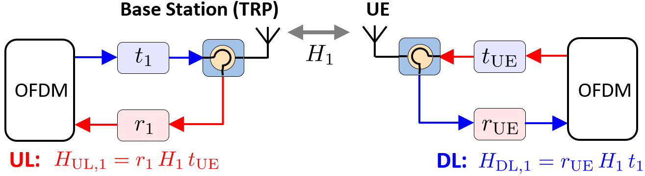
Figure 1: Reciprocity only holds for propagation channel $H_{1}$, but the UL channel and DL channel are different because of differences in TX and RX.

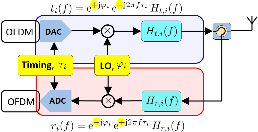
Figure 2: The LO effect on the TX chain is $+\varphi$ while for the RX chain it is $-\varphi$. A similar relationship exists for timing errors.

Figure 1 shows a simplified block diagram of a TDD transmission system. In UL direction, the signal goes through UE TX chain $t_{\text{UE}}$, reciprocal propagation channel $H_{1}$ (which includes everything between the two circulators, i.e., also antenna, feeding network, RF filters etc.) and base station RX chain $r_{1}$. The DL can be described in a similar way, so that UL channel $H_{\text{UL},1}$ and DL channel $H_{\text{DL},1}$ can be written as:

$$H_{\text{UL},1} =r_{1}\,H_{1}\,t_{\text{UE}}$$ (1)

$$H_{\text{DL},1} =r_{\text{UE}}\,H_{1}\,t_{1}.$$ (2)

The TX and RX chains can be further decomposed into:

$$t_{i}(f) =\mathrm{e}^{+\mathrm{j}\varphi_{i}}\,\mathrm{e}^{-\mathrm{j}2\pi f\tau_{i}}\,H_{t,i}(f)$$ (3)

$$r_{i}(f) =\mathrm{e}^{-\mathrm{j}\varphi_{i}}\,\mathrm{e}^{+\mathrm{j}2\pi f\tau_{i}}\,H_{r,i}(f),$$ (4)

as also illustrated in Figure 2 and formally proven in the appendix. It is important to emphasize here that $t_{i}$ and $r_{i}$ are mathematical constructs and only the product $r_{j}t_{i}$ has real physical meaning. Note that (3) and (4) provide a general description of the $i$-th Transceiver (TRX) and can be used to describe the TRX at the base station but also at the UE, though for clarity the subscript “UE” is used for the latter. Moreover, $t_{i}(f)$ and $r_{i}(f)$ now include a frequency dependency $f$ because of Orthogonal Frequency Division Multiplexing (OFDM) [10], where subcarriers at frequency $f=Fl$ are transmitted in parallel, with $F$ denoting the subcarrier spacing and $l$ the subcarrier index, as explained in more detail in the appendix. To simplify the explanation, however, the frequency dependency will be ignored from now on, but one must keep in mind that there are many more subcarriers. The variable $\varphi_{i}$ in (3) and (4) describes the LO phase, $\tau_{i}$ the timing offset and $H_{t,i}$ includes the “obvious” HW elements of the transmitter chain, such as power amplifiers and filters, but also the less obvious elements, such as the additional delay from the common LO phase $\varphi_{i}$ to the actual LO phase used for up-conversion, i.e., $\varphi_{t,i}=\varphi_{i}+\Delta\varphi_{t,i}$. The variable $H_{r,i}$ is similar to $H_{t,i}$, but for the RX chain. Typically $H_{r,i}$ and $H_{t,i}$ will be relatively stable over time (e.g., hours, depending mainly on temperature variations) while $\varphi_{i}$ and $\tau_{i}$ might change very fast, especially for free-running LOs (e.g., $100\,\text{\textmu s}$, depending of course on HW quality and implementation).

The key difference of (3) and (4) compared with the TX and RX model of other papers [3, 4, 5, 6] is the different sign in the RX chain (and the inclusion of time offsets):

$$\begin{matrix}\textbf{Inaccurate}\,\text{[3]-[6]}&&&&&\textbf{Correct}\\ t_{i}\propto\mathrm{e}^{+\mathrm{j}\varphi_{i}}&&&&&t_{i}\propto\mathrm{e}^{+\mathrm{j}\varphi_{i}}\\ r_{i}\propto\mathrm{e}^{+\mathrm{j}\varphi_{i}}&&&&&r_{i}\propto\mathrm{e}^{-\mathrm{j}\varphi_{i}}\end{matrix}.$$ (5)

The formal proof for (5) can be found in the appendix, while in the following let us consider a more intuitive explanation. For the sake of argument, all other components except the LO are ignored:

• Suppose TX and RX of the same TRX are directly connected together. One would expect that the transfer function becomes “1” because up-conversion and down-conversion perfectly cancels each other and there are no other components in this example. The only way how this can happen is by $\mathrm{e}^{-\mathrm{j}\varphi}\mathrm{e}^{+\mathrm{j}\varphi}=1$, i.e., the LO influence on TX and RX chain must have different signs.

• An absolute phase does not exist, one can only define relative phases. Thus, the transmission from TX to RX must be invariant to any common phase transformation of the form $\varphi\rightarrow\varphi^{\prime}+b$, which is only possible if the LO effect on TX and RX have different signs.

III Implications of TX and RX Model

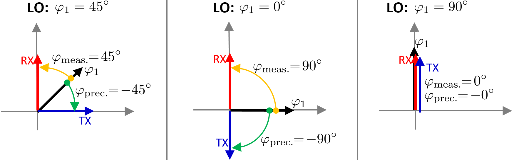
Figure 3: Depending on the LO phase, the phase of the precoded TX signal can be completely different, implying that calibration between TRPs is of upmost importance for coherent joint transmission.

Let us first consider a simple example to show how severe the LO effect is once the correct TX and RX model is used. As illustrated in Figure 3, a reference RX signal with a “global” phase of $\varphi_{\text{RX}}=90^{\circ}$ is assumed. One cannot measure this “global” phase, only $\varphi_{\text{meas.}}=\varphi_{\text{RX}}-\varphi_{1}=45^{\circ}$ (left picture) can be measured, i.e., relative to the LO. The precoded signal is then the conjugate of the measured RX signal, $\varphi_{\text{prec.}}=-\varphi_{\text{meas.}}=-45^{\circ}$. When sending out this signal, it will again be relative to the LO, i.e., the “global” TX phase is $\varphi_{\text{TX}}=\varphi_{\text{prec.}}+\varphi_{1}=0^{\circ}$. Suppose this is exactly the “global” TX phase which adds up coherently with the signal of another TRP at the UE, i.e., everything is calibrated. If now the LO phase of TRP1 drifts to $\varphi_{1}=0^{\circ}$ (middle picture), while everything else stays constant, coherency will be lost. This can easily be seen by repeating the same procedure as before, i.e., measure the RX signal $\varphi_{\text{meas.}}=90^{\circ}$ and send the conjugate of it $\varphi_{\text{prec.}}=-90^{\circ}$, leading to a “global” TX phase of $\varphi_{\text{TX}}=-90^{\circ}$. If the system was coherent before, this coherency is now broken. Even more surprising, if the old channel estimation would have been used, $\varphi_{\text{meas.}}=45^{\circ}$, the overall TX phase error would be smaller. This simple example illustrates that whenever the LO phases drift apart, a new calibration becomes necessary.

III-A Relative Reciprocity Calibration: Why Free-Running LOs are Not Useful

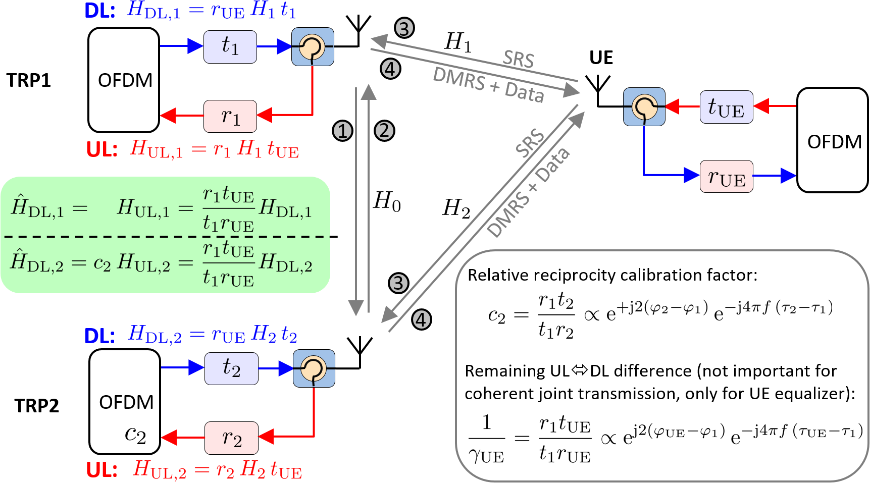
Figure 4: Concept of relative reciprocity calibration. The extension to more TRX, TRPs and UEs is trivial and thus omitted.

As already described above, coherent joint transmission requires reciprocity calibration. A practical method to achieve that is Over The Air (OTA) relative reciprocity calibration [9], where one TRX acts as a reference. Without loss of generality, let us consider two TRPs and one UE, as illustrated in Figure 4. By combining (1) and (2), the UL channel can be expressed by the DL channel according to:

$${\hat{H}}_{\text{DL,1}}=\ \ \ {H}_{\text{UL,1}} =\frac{r_{1}t_{\text{UE}}}{t_{1}r_{\text{UE}}}{H}_{\text{DL,1}}$$ (6)

$${\hat{H}}_{\text{DL,2}}=c_{2}\,{H}_{\text{UL,2}} =\frac{r_{1}t_{\text{UE}}}{t_{1}r_{\text{UE}}}{H}_{\text{DL,2}}.$$ (7)

For TRP1, the estimated DL channel, ${\hat{H}}_{\text{DL,1}}$, is directly given by the UL channel estimate (assumed to be perfectly known), i.e., this is our reference TRX. If the same method would be applied for TRP2, coherency cannot be guaranteed because of the different factors $\frac{r_{1}}{t_{1}}$ at TRP1 and $\frac{r_{2}}{t_{2}}$ at TRP2. Thus, calibration becomes necessary, i.e., we have to multiply the UL channel estimate at TRP2 with the relative reciprocity calibration factor $c_{2}=\frac{r_{1}t_{2}}{t_{1}r_{2}}$. This calibration is relative in the sense that the signals of the two TRPs will add up coherently at the UE, but with some unknown common phase rotation $(\frac{r_{1}t_{\text{UE}}}{t_{1}r_{\text{UE}}})^{*}$, which needs to be estimated by the UE e.g., by DMRS. Calibration factor $c_{2}$ can be obtained by sending a signal from TRP1 to TRP2 in time-slot 1, delivering measurement $y_{2,1}[1]$. In a second time-slot, TRP2 will send a calibration signal to TRP1, delivering measurement $y_{1,2}[2]$:

$$y_{2,1}[1] =r_{2}\,H_{0}\,t_{1}$$ (8)

$$y_{1,2}[2] =r_{1}\,H_{0}\,t_{2}.$$ (9)

By dividing those measurement results, the relative reciprocity calibration factor $c_{2}$ becomes,

$$c_{2}(f) =\frac{y_{1,2}[2]}{y_{2,1}[1]}=\frac{r_{1}H_{0}t_{2}}{t_{1}H_{0}r_{2}}=\frac{r_{1}t_{2}}{t_{1}r_{2}}$$ (10)

$$=\mathrm{e}^{+\mathrm{j}2(\varphi_{2}-\varphi_{1})}\,\mathrm{e}^{-\mathrm{j}4\pi f\,(\tau_{2}-\tau_{1})}\frac{H_{r,1}(f)\,H_{t,2}(f)}{H_{r,2}(f)\,H_{t,1}(f)}.$$ (11)

Note that a stable channel and a stable HW is assumed in (10), the more general solution would include time variations of $r$, $t$ and $H_{0}$, but is omitted here for the sake of clarity.

The implications of (11) are significant. As soon as the LO phases $\varphi_{2}-\varphi_{1}$ drift apart, a new reciprocity calibration becomes necessary, otherwise coherency is lost. In the most straightforward approach, the number of OTA calibration signals is proportional to the number of uncalibrated TRX [9]. While this simple approach can be improved, e.g., signals can be frequency multiplexed or avalanche-like methods can be employed [11], the calibration overhead for free-running LOs is still very large and completely unnecessary. Simply by locking the LO phases to some common reference clock, most of the problems can be avoided. Thus, the clear recommendation is to lock LOs as much as possible. In a distributed MIMO setup, locking LOs is of course more challenging but one can still distribute a common clock signal over cable (e.g., clock recovery). However, time variations of the long cable (e.g., because of temperature variations) will also cause LO phase drifts, implying that reciprocity calibration needs to be performed more frequently than in a pure massive MIMO system, but still less often than for free-running LOs.

Note that in this paper timing errors $\tau_{2}-\tau_{1}$ will be ignored since they typically have less impact on phase errors when compared with the LO, i.e., Low Frequency (LF) vs. Radio Frequency (RF), but of course this depends on HW implementation and could also be a major problem.

III-B Perfect Reciprocity Calibration: A Problematic Assumption

A common assumption in literature is perfect reciprocity calibration, i.e., the DL channel can be perfectly estimated from the UL channel (ignoring noise and interference). Considering (6) and (7), this can be achieved if all TRPs know UE reciprocity calibration factor $\gamma_{\text{UE}}$, so that

$${\hat{H}}_{\text{DL,1}}=\ \ \ \gamma_{\text{UE}}\,{H}_{\text{UL,1}} ={H}_{\text{DL,1}}$$ (12)

$${\hat{H}}_{\text{DL,2}}=\gamma_{\text{UE}}\,c_{2}\,{H}_{\text{UL,2}} ={H}_{\text{DL,2}},$$ (13)

with

$$\gamma_{\text{UE}}(f) =\frac{t_{1}r_{\text{UE}}}{r_{1}t_{\text{UE}}}$$ (14)

$$=\mathrm{e}^{-\mathrm{j}2(\varphi_{\text{UE}}-\varphi_{1})}\,\mathrm{e}^{\mathrm{j}4\pi f\,(\tau_{\text{UE}}-\tau_{1})}\frac{H_{r,\text{UE}}(f)\,H_{t,1}(f)}{H_{r,1}(f)\,H_{t,\text{UE}}(f)}$$ (15)

Similar to the relative reciprocity calibration factor, the implications of (15) are severe. As soon as the LO phases $\varphi_{\text{UE}}-\varphi_{1}$ drift apart, perfect reciprocity calibration is lost and simple blind DL channel estimation no longer works. Sending more SRS symbols also does not help, it actually worsens the performance. Thus, one needs to measure the UE reciprocity calibration factor again, but this is usually quite cumbersome: Firstly, the UE needs to measure the phase of the effective DL channel by DMRS, i.e., $\arg\{1/\gamma_{\text{UE}}^{*}\}=\arg\{\gamma_{\text{UE}}\}$. Secondly, it needs to feedback this information to the TRPs, wasting UL resources. Finally, the TRP can change the TX phase so that the signal arrives at the UE with phase zero (assuming everything was stable enough so that the feedback delay has no influence). However, if the UE has already estimated the effective DL channel, it can use this information directly for equalization and there is simply no point in sending back this information. Only in the unrealistic case of a very stable $\varphi_{\text{UE}}-\varphi_{1}$, perfect reciprocity calibration might have some advantages in some scenarios, but considering the very good alternative of relative reciprocity calibration together with low overhead and robust DMRS, which not only track the LO phases but also time variations of the propagation channel, the whole concept of perfect reciprocity calibration seems not very useful.

III-C SRS and DMRS

SRS and DMRS have been mentioned several times, so let us quickly look at those reference signals. The purpose of SRS is to estimate the full UL channel matrix, i.e., $\mathbf{H}_{\text{UL}}\in\mathbb{C}^{N_{\text{TRX}}\times N_{\text{UEs}}}$, and requires a minimum of $N_{\text{UEs}}$ orthogonal time-frequency resources, though sending more SRS and averaging out noise and interference can be advantageous. DMRS, on the other hand, are intermixed within the Quadrature Amplitude Modulation (QAM) data symbols (they use the same precoder) and allow to estimate the effective DL channel at the UE, $\mathbf{a}=\text{diag}\{\mathbf{H}_{\text{DL}}\mathbf{W}\}\in\mathbb{C}^{N_{\text{UEs}}\times 1}$, with $\mathbf{W}\in\mathbb{C}^{N_{\text{TRX}}\times N_{\text{UEs}}}$ denoting the precoder. A minimum of only one time-frequency resource is required to estimate all elements of $\mathbf{a}$, though sending more DMRS and averaging out noise and interference can again be advantageous. For example, spending only one time-frequency position for DMRS, there is a channel estimation penalty of roughly 3dB (1+1/1) on the Signal-to-Interference plus Noise Ratio (SINR), while for averaging over six time-frequency position, as used in 5G as one possible configuration (within 12 subcarriers and 14 OFDM symbols), the penalty is only 0.7dB (1+1/6). Thus, the overhead of DMRS is very low, while the performance very good, explaining why they are so useful.

IV Numerical Example

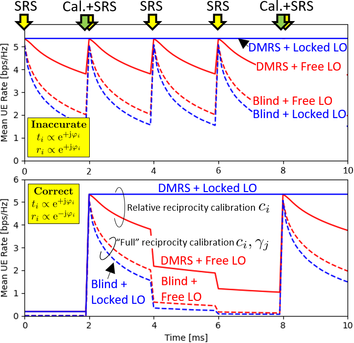
Figure 5: The correct TX and RX model leads to completely different conclusions when compared with the inaccurate model. All LOs used for coherent joint transmission should be locked. Moreover, relative reciprocity calibration together with DMRS offer a very good performance.

The numerical example shown in Figure 5 is based on a similar setup as [6]. In total there are 16 TRPs, each with 64 TRXs. Four TRPs form a distributed massive MIMO cluster and the total network consists of $10\times 16=160$ UEs. The phase noise model is the same as in [12], i.e., $\varphi[n]=\varphi[n-1]+\Delta$, with $\Delta\sim\mathcal{N}(0,\sigma^{2}=0.01)$ and $n$ representing the time index (sampling time $T_{\text{S}}=100\,\text{\textmu s}$). Moreover, zero-forcing precoding is assumed, the LO phases have a random initial value, no other HW effects are present, i.e., $\tau_{i}=0,H_{t,i}=H_{r,i}=1$, and perfect channel estimation (SRS and DMRS) is available. When using the inaccurate TRX model, reciprocity calibration is not needed because the LO phases become part of the channel and will be implicitly estimated by SRS. On the other hand, with the correct model, reciprocity calibration is of upmost importance. Free-running LOs and blind DL channel estimation are both not very useful because they would require continuous calibration signals and have overall a very poor performance. Instead, all LOs used for coherent joint transmission should be locked and relative reciprocity calibration together with DMRS employed.

V Conclusions

Some common misunderstandings related to reciprocity calibration have been clarified in this paper. Essentially, coherent joint transmission can only work if the LO phases are locked, either directly by “cables” or indirectly by continuously sending reciprocity calibration signals. The first method is typically preferred as it does not “waste” any time-frequency resources. The commonly made assumption of perfect reciprocity calibration typically does not hold, as it would require too much calibration overhead. Instead, relative reciprocity calibration is a better option. Thus, to make blind DL channel estimation at the UE practically useful, one must also be able to blindly estimate the phase, mostly ignored in literature so far. Alternatively, by sending low-overhead DMRS many problems can be avoided and is therefore the recommended solution for effective DL channel estimation at the UE.

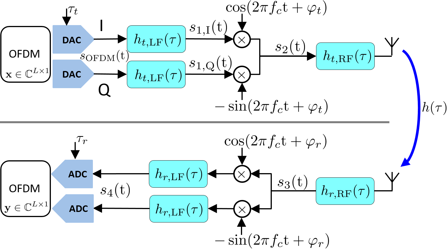
Figure 6: Block diagram of a generic transmission chain, used to derive the TX and RX transfer functions $t_{i}$ and $r_{i}$.

Figure 6 shows a generic transmission chain, used to mathematically proof the simplified TX and RX model in (3) and (4). Note that all elements in Figure 6 are assumed to be perfect in order to focus on the key aspects, i.e., perfectly linear, no IQ imbalances, no phase noise within one OFDM symbol, etc. The transmitted OFDM signal in the time domain, $s_{\text{OFDM}}(\text{t})$, can be written as [10],

$$s_{\text{OFDM}}(\text{t})=\sum_{l=-\frac{L}{2}}^{\frac{L}{2}-1}\mathrm{e}^{\mathrm{j}2\pi\,lF\,(\text{t}-\tau_{t})}\,x_{l},$$ (16)

where $x_{l}$ denotes the transmitted QAM data symbol at subcarrier position $l$, $F$ the subcarrier spacing, $L$ the total number of subcarriers, and $\tau_{t}$ the delay of starting the transmission (vs. a perfect “global” time reference). Note that the rectangular window function of OFDM is ignored in (16), which is fine as long as the cyclic prefix is sufficiently long. The I-signal experiences the real valued impulse response $h_{t,\text{LF}}(\tau)$, leading to,

$$\begin{split}s_{1,\text{I}}(\text{t})&=\Re\{s_{\text{OFDM}}(\text{t})\}\ast h_{t,\text{LF}}(\text{t})\\ &=\Re\Big{\{}\sum_{l=-\frac{L}{2}}^{\frac{L}{2}-1}\mathrm{e}^{\mathrm{j}2\pi\,lF\,(\text{t}-\tau_{t})}x_{l}\underbrace{\int\limits_{-\infty}^{\infty}h_{t,\text{LF}}(\tau)\mathrm{e}^{-\mathrm{j}2\pi\,lF\,\tau}\mathrm{d}\tau}_{H_{t,\text{LF}}(lF)}\Big{\}}\end{split},$$ (17)

with $H_{t,\text{LF}}(f)$ denoting the transfer function of $h_{t,\text{LF}}(\tau)$, i.e., its Fourier transform. The Q-signal, $s_{1,\text{Q}}(\text{t})$, is similar except for taking the imaginary part instead of the real part. Utilizing Euler’s formula, the up-converted signal can be written as:

$$\begin{split}s_{2}(\text{t})&=s_{1,\text{I}}(\text{t})\cos(2\pi f_{c}\text{t}+\varphi_{t})-s_{1,\text{Q}}(\text{t})\sin(2\pi f_{c}\text{t}+\varphi_{t})\\ &=\Re\Big{\{}\mathrm{e}^{\mathrm{j}\varphi_{t}}\sum_{l=-\frac{L}{2}}^{\frac{L}{2}-1}\mathrm{e}^{\mathrm{j}2\pi(lF+f_{c})\text{t}}\,\mathrm{e}^{-\mathrm{j}2\pi lF\tau_{t}}\,H_{t,\text{LF}}(lF)\,x_{l}\Big{\}},\end{split}$$ (18)

with $f_{c}$ denoting the carrier frequency. The convolution of $s_{2}(\text{t})$, TX RF chain $h_{t,\text{RF}}(\tau)$, propagation channel $h(\tau)$ and RX RF chain $h_{r,\text{RF}}(\tau)$ leads to $s_{3}(\text{t})=s_{2}(\text{t})\ast h_{t,\text{RF}}(\text{t})\ast h(\text{t})\ast h_{r,\text{RF}}(\text{t})$, which can be similarly described as in (17), i.e., using their Fourier transforms. Again, employing Euler’s formula, the baseband signal $s_{4}(\text{t})$ can be written as,

$$\begin{split}s_{4}(\text{t})&=h_{r,\text{LF}}(\text{t})\ast s_{3}(t)[\cos(2\pi f_{c}\text{t}+\varphi_{r})-\mathrm{j}\sin(2\pi f_{c}\text{t}+\varphi_{r})]\\ &=\frac{1}{2}\mathrm{e}^{\mathrm{j}\varphi_{t}}\mathrm{e}^{-\mathrm{j}\varphi_{r}}\sum_{l=-\frac{L}{2}}^{\frac{L}{2}-1}\mathrm{e}^{\mathrm{j}2\pi lF\,\text{t}}\,\mathrm{e}^{-\mathrm{j}2\pi lF\tau_{t}}\,H_{t,\text{LF}}(lF)\\ &\quad\ H_{t,\text{RF}}(lF+f_{c})\,H(lF+f_{c})\,H_{r,\text{RF}}(lF+f_{c})\\ &\quad\ H_{r,\text{LF}}(lF)\,x_{l}\,+\frac{1}{2}\mathrm{e}^{-\mathrm{j}4\pi f_{c}\text{t}}z(\text{t}),\end{split}$$ (19)

where $z(\text{t})$ is not relevant because it will be averaged out later. Finally, received data symbol $y_{l}$ can be obtained by OFDM demodulation (assumed to be delayed by $\tau_{r}$) according to,

$$\begin{split}y_{l}&=2F\!\!\!\int\limits_{\tau_{r}}^{\tau_{r}+\frac{1}{F}}\!\!\!s_{4}(\text{t})\mathrm{e}^{-\mathrm{j}2\pi\,lF\,(\text{t}-\tau_{r})}\mathrm{d}\text{t}\\ &=r(lF)\,H(lF+f_{c})\,t(lF)\,x_{l},\end{split}$$ (20)

with

$$t(lF) =\mathrm{e}^{\mathrm{j}\varphi_{t}}\,\mathrm{e}^{-\mathrm{j}2\pi lF\tau_{t}}\,H_{t,\text{LF}}(lF)\,H_{t,\text{RF}}(lF+f_{c})$$ (21)

$$r(lF) =\mathrm{e}^{-\mathrm{j}\varphi_{r}}\,\mathrm{e}^{\mathrm{j}2\pi lF\tau_{r}}H_{r,\text{LF}}(lF)\,H_{r,\text{RF}}(lF+f_{c}).$$ (22)

Within one TRX, the LO phases and time delays will be derived from the same common reference,

$$\begin{matrix}\varphi_{t}=\varphi_{i}+\Delta\varphi_{t}&&&&\tau_{t}=\tau_{i}+\Delta\tau_{t}\\ \varphi_{r}=\varphi_{i}+\Delta\varphi_{r}&&&&\tau_{r}=\tau_{i}+\Delta\tau_{r}\end{matrix}.$$ (23)

Combining (21), (22) and (23) directly leads to $t_{i}(f)$ and $r_{i}(f)$, presented in the main text, see (3) and (4).

References

- [1] E. Dahlman, S. Parkvall, and J. Skold, 5G NR: The next generation wireless access technology. Academic Press, 2020.
- [2] E. Björnson, J. Hoydis, and L. Sanguinetti, “Massive MIMO networks: Spectral, energy, and hardware efficiency,” Foundations and Trends in Signal Processing, vol. 11, no. 3-4, pp. 154–655, 2017.
- [3] M. R. Khanzadi, G. Durisi, and T. Eriksson, “Capacity of SIMO and MISO phase-noise channels with common/separate oscillators,” IEEE Transactions on Communications, vol. 63, no. 9, pp. 3218–3231, 2015.
- [4] R. Krishnan et al., “Linear massive MIMO precoders in the presence of phase noise—a large-scale analysis,” IEEE Transactions on Vehicular Technology, vol. 65, no. 5, pp. 3057–3071, 2015.
- [5] W. Jiang and H. D. Schotten, “Impact of channel aging on zero-forcing precoding in cell-free massive MIMO systems,” IEEE Communications Letters, vol. 25, no. 9, pp. 3114–3118, 2021.
- [6] E. Björnson, M. Matthaiou, A. Pitarokoilis, and E. Larsson, “Distributed massive MIMO in cellular networks: Impact of imperfect hardware and number of oscillators,” in EUSIPCO, 2015, pp. 2436–2440.
- [7] A. K. Papazafeiropoulos, “Impact of general channel aging conditions on the downlink performance of massive MIMO,” IEEE Transactions on Vehicular Technology, vol. 66, no. 2, pp. 1428–1442, 2016.
- [8] H. Q. Ngo and E. G. Larsson, “No downlink pilots are needed in TDD massive MIMO,” IEEE Transactions on Wireless Communications, vol. 16, no. 5, pp. 2921–2935, 2017.
- [9] C. Shepard, H. Yu, N. Anand, E. Li, T. Marzetta, R. Yang, and L. Zhong, “Argos: Practical many-antenna base stations,” in Proc. 18th conference on Mobile computing and networking, 2012, pp. 53–64.
- [10] R. Nissel, “Filter bank multicarrier modulation for future wireless systems,” Dissertation, TU Wien, 2017.
- [11] X. Jiang et al., “A framework for over-the-air reciprocity calibration for TDD massive MIMO systems,” IEEE Transactions on Wireless Communications, vol. 17, no. 9, pp. 5975–5990, 2018.
- [12] H. Mehrpouyan et al., “Joint estimation of channel and oscillator phase noise in MIMO systems,” IEEE Transactions on Signal Processing, vol. 60, no. 9, pp. 4790–4807, 2012.