Anatomy of kaon decays and prospects for lepton flavour universality violation

Abstract

The kaon sector is characterised by several processes which are under active investigation across different experiments. In this work, we present the global picture that emerges from a study of the different decay modes. We begin by revisiting the theoretical component of these decays and providing up-to-date predictions of the Standard Model as well as the corresponding uncertainties. Several new features emerge, in particular for $K_{S,L}\to\mu\bar{\mu}$, and are presented in considerable detail. This offers an ideal platform for extracting the parameter space supported by the existing data. Motivated by possible lepton flavour universality violation in $B$ decays, we investigate such Beyond the Standard Model effects also in rare kaon decays. Without loss of generality, our primary analyses correspond to the paradigm where the Wilson coefficients for operators involving tau leptons are chosen to be equal to that involving the muon, i.e. $\delta C^{\tau}=\delta C^{\mu}$. We conclude by presenting the possible picture that can be achieved towards the end of the run of data accumulation in the planned experiments. This includes assumptions on possible sensitivity goals that the experiments can aim to achieve, in order to extract the kind of physics highlighted in this paper.

1 Introduction

The last decade has seen a period of intense scrutiny for the flavour structure of the Standard Model (SM). The plethora of experimental results has served as a catalyst to investigate the different sectors, both from the SM point of view as well as looking at possible effects of New Physics (NP) on them. Some of the different measurements which drive the interest in the theoretical community include the anomalous magnetic moment of the muonAbi:2021gix ; Bennett:2006fi , decays corresponding to $b\to s$ transitions ($B$ physics) LHCb:2014vgu ; LHCb:2017avl ; Belle:2019oag ; LHCb:2019hip ; LHCb:2021trn , $b\to c$ transitions BaBar:2013mob ; Belle:2015qfa ; LHCb:2015gmp ; LHCb:2017smo ; Belle:2019gij ; LHCb:2022piu , nuclear beta decays and implications for $V_{ud}$ Hardy:2020qwl , as well as decays corresponding to $s\to d$ transitions (kaon physics) NA62:2021zjw ; Bician:2020ukv ; Ahn:2018mvc . Many of these experiments have hinted at the possibility of non-standard physics in their respective data analysed thus far. Among the most interesting hints of New Physics is the observation of lepton flavour universality violation (LFUV) in rare $B$ decays LHCb:2014vgu ; LHCb:2017avl ; Belle:2019oag ; LHCb:2019hip ; LHCb:2021trn . Global fits using the effective field theory approach proved useful in constructing the appropriate beyond the SM scenarios to explain LFUV Hurth:2021nsi ; Alguero:2021anc ; Altmannshofer:2021qrr ; Ciuchini:2020gvn ; Geng:2021nhg ; Datta:2019zca ; Alok:2019ufo ; Kowalska:2019ley ; DAmico:2017mtc . It is natural to expect that these NP effects would also impact operators contributing to kaon decays. This provides a strong motivation to consider an effective theory fit dedicated to kaons and to possibly achieve a similar sensitivity to the corresponding analyses in $B$ decays.

There are several observables in $K$ systems that have the capability to make an individual impact on the eventual global fits. Recently, there has been a significant (and ongoing) experimental effort focused on the measurements of the branching fractions of $K^{+}\to\pi^{+}\nu\bar{\nu}$ (NA62 at CERN NA62:2021zjw ) and $K_{L}\to\pi^{0}\nu\bar{\nu}$ (KOTO at J-PARC Ahn:2018mvc ). Both of them have negligible uncertainty on long-distance contributions, making them highly sensitive to non-standard physics. However, any analysis involving only these decays proves inadequate to make concrete claims about LFUV effects in kaons, thereby prompting the addition of new observables. In the context of direct sensitivity to LFUV, $K^{+}\to\pi^{+}\ell\bar{\ell}$ offers an exciting prospect. It has been shown that the difference of the leading order polynomial expansion coefficients of the vector form factor in these decays is sensitive to short-distance flavour violating effects Crivellin:2016vjc . The parameter space that is permitted by these three observables can be further limited by the consideration of decays like $K_{L,S}\to\ell\bar{\ell}$ and $K_{L}\to\pi^{0}\ell\bar{\ell}$. With the exception of $K_{L}\to\mu\bar{\mu}$, the others have only upper bounds with respect to their experimental status. While they are weak at present, they are still useful in drawing attention to a specific part of the parameter space of the NP Wilson coefficients. Each of them ($K_{L,S}\to\ell\bar{\ell}$, $K_{L}\to\pi^{0}\ell\bar{\ell}$) is characterised by dominant long-distance effects, making it relatively more challenging to extract non-standard physics. This translates into a limitation on the existing accuracy in their SM computation. However, there exists a well-defined experimental program for each of these decays. This may either imply an improvement in the existing sensitivities or a measurement at the SM level and is outlined in the third column of table 2.

In light of several ongoing and planned measurements for decays in the kaon sector, this paper intends to demonstrate the complementary capability for LFUV measurements in kaon systems. We analyse each of these decays and make a careful evaluation of the theoretical uncertainties. Using the updated values from CKM and other input parameters, the uncertainties are computed using a Monte Carlo approach. An interesting difference from past literature is observed for the $K_{L}\to\mu\bar{\mu}$ decay which is described by asymmetric uncertainties. Integrating these decays in SuperIso Mahmoudi:2007vz ; Mahmoudi:2008tp ; Mahmoudi:2009zz ; Neshatpour:2021nbn ; Neshatpour:2022fak , the relevant parameter space of the New Physics Wilson coefficients is identified. Guided by a well-defined strategy for the measurement of many of these decays, the experimental uncertainties are used appropriately. Furthermore, for decays for which no such well-defined strategy exists, we also present projections on the progress on the experimental side. Demonstrating a rich yield of interesting physics could motivate modified strategies for such decays in the future. This is particularly true for the measurement of vector form factors in $K^{+}\to\pi^{+}\ell\bar{\ell}$. While measurements of these form factors exist for both the electron  E865:1999ker ; NA482:2009pfe ; NA482:2010zrc and the muon Bician:2020ukv , a strong case for higher precision measurements of these quantities is presented in this work. Similarly, our results present the need for a reduction in the error on the theoretical computation of $K_{L}\to\mu\bar{\mu}$.

The paper is organised as follows: in section 2 we analyse the decay modes of interest in considerable detail. The considered processes are $K^{+}(K_{L})\to\pi^{+}(\pi^{0})\nu\bar{\nu}$ in section 2.1, LFUV in $K^{+}\to\pi^{+}\ell\ell$ decays in section 2.2, $K_{S,L}\to\mu\bar{\mu}$ in section 2.3 and $K_{L}\to\pi^{0}\ell\bar{\ell}$ in section 2.4. The analyses in each of these subsections (along with the appendices) are self-contained and offer an up-to-date evaluation of the SM values as well as the corresponding uncertainties. In section 3 we present a global picture involving all the decays, which illustrates the existing bounds from the different observables. Section 3.1 is devoted to the description of the methodology of our fit. In section 3.2 we perform a global fit to current experimental data. Section 3.3 offers possible improvements in the fits at the end of the run for most of the experiments. This includes using the official projections for some observables as well as choosing optimistic reaches for the others. Finally, we conclude in section 4.

2 Theoretical framework

In this section, we set up the convention to be followed for the rest of the paper. The $s\to d$ transitions can be parameterised by the following effective Hamiltonian:

$$\mathcal{H}_{\rm eff}=-\frac{4G_{F}}{\sqrt{2}}\lambda_{t}^{sd}\frac{\alpha_{e}}{4\pi}\sum_{k}C_{k}^{\ell}O_{k}^{\ell}\,,$$ (1)

where $\lambda_{t}^{sd}\equiv V^{*}_{ts}V_{td}$ and the relevant effective operators are

$${O}_{9}^{\ell}=(\bar{s}\gamma_{\mu}P_{L}d)\,(\bar{\ell}\gamma^{\mu}\ell)\,, {O}_{10}^{\ell}=(\bar{s}\gamma_{\mu}P_{L}d)\,(\bar{\ell}\gamma^{\mu}\gamma_{5}\ell)\,,$$

$${O}_{L}^{\ell}=(\bar{s}\gamma_{\mu}P_{L}d)\,(\bar{\nu}_{\ell}\,\gamma^{\mu}(1-\gamma_{5})\,\nu_{\ell})\,,$$ (2)

with $P_{L}=(1-\gamma_{5})/2$. The most general Hamiltonian also includes scalar and pseudoscalar operators, as well as the chirality-flipped counterpart of the above operators where the quark currents are right-handed. In this instance, we focus on this small subset of operators which have the same structure as the most relevant operators for explaining the neutral current $B$-anomalies LHCb:2014vgu ; LHCb:2017avl ; Belle:2019oag ; LHCb:2019hip ; LHCb:2021trn . The Wilson coefficients $C_{k}^{\ell}$ include any potential (flavour violating) New Physics contribution parameterised as

$$C_{k}^{\ell}=C_{k,{\rm SM}}^{\ell}+\delta C_{k}^{\ell}\,.$$ (3)

In recent years, there has been much progress in the measurements of rare kaon decays. However, still several of the rare kaon decays have not been observed and there are only upper bounds available for them. In general, different New Physics contributions with various combinations of the operator structures of eq. 2 can contribute to kaon decays. Nonetheless, given the rather limited experimental data currently available for rare kaon decays and the fact that New Physics is more conveniently explored in the chiral basis, we limit our analysis to the class of NP scenarios where the charged and neutral leptons are related to each other by the SU(2)_L gauge symmetry. As we consider only left-handed quark currents, the different Wilson coefficients that we consider are related to each other as $\delta C_{L}^{\ell}\equiv\delta C_{9}^{\ell}=-\delta C_{10}^{\ell}$. With this background, we set up the theoretical description of the different decay modes in the following subsections.

2.1 $K^{+}\to\pi^{+}\nu\bar{\nu}$ and $K_{L}\to\pi^{0}\nu\bar{\nu}$

These rare decay modes receive dominant short-distance (SD) contributions. Their high sensitivity to any NP effect while having very small theoretical uncertainties justify their status as being among the eagerly awaited measurements from the corresponding experiments NA62:2021zjw ; Ahn:2018mvc . In the notation discussed above, the branching fractions for these modes are given as Bobeth:2017ecx (see also Rein:1989tr ; Hagelin:1989wt ; Lu:1994ww ; Geng:1995np ; Buchalla:1995vs ; Fajfer:1996tc ; Buchalla:1996fp ; Buchalla:1998ba ; Mescia:2007kn ; Misiak:1999yg ; Brod:2010hi )

$${\rm BR}(K_{L}\to\pi^{0}\nu\bar{\nu}) =\frac{\kappa_{L}}{\lambda^{10}}\frac{1}{3}s_{W}^{4}\sum_{\ell}{\rm Im}^{2}\left[\lambda_{t}C_{L}^{\ell}\right]\,,$$ (4)

$${\rm BR}(K^{+}\to\pi^{+}\nu\bar{\nu}) =\frac{\kappa_{+}(1+\Delta_{\rm EM})}{\lambda^{10}}\frac{1}{3}s_{W}^{4}\sum_{\ell}\left[{\rm Im}^{2}\Big{(}\lambda_{t}C_{L}^{\ell}\Big{)}+{\rm Re}^{2}\Big{(}-\frac{\lambda_{c}X_{c}}{s_{W}^{2}}+\lambda^{sd}_{t}C_{L}^{\ell}\Big{)}\right]\,,$$ (5)

where the sum is over the three neutrino flavours. Considering the relevant input parameters as collected in appendix A, we calculate the short-distance SM contribution given by $X_{c}$ and $C_{L,{\rm SM}}^{\ell}=C_{L,{\rm SM}}={-X(x_{t})}/{s_{W}^{2}}$ (see appendix B). The values of the branching fraction for the SM, corresponding to these inputs are given in table 2 where the theory uncertainties are estimated using a Monte Carlo method, assuming Gaussian errors for the input parameters.

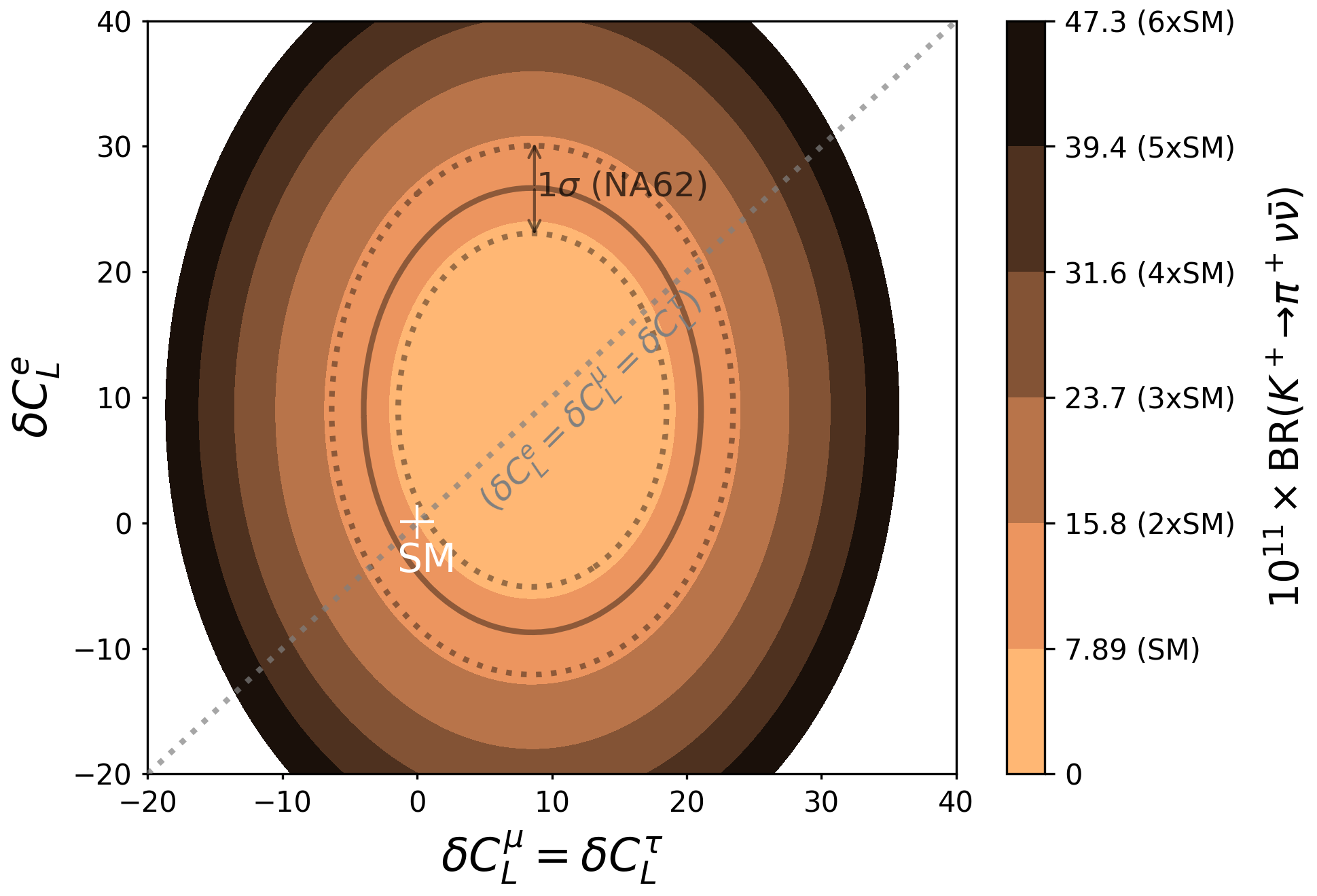
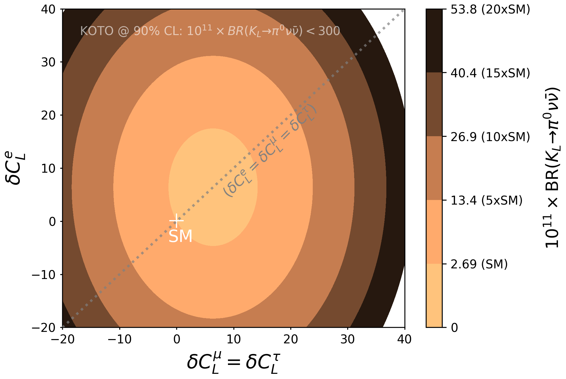
Figure 1: BR($K^{+}\to\pi^{+}\bar{\nu}\nu$) (left) and BR($K_{L}\to\pi^{0}\bar{\nu}\nu$) (right) as a function of $\delta C_{L}^{e}$ and $\delta C_{L}^{\mu}=\delta C_{L}^{\tau}$. The dotted grey line represents the lepton flavour universality scenario. In the left plot, the brown solid (dotted) line corresponds to the measured central value ($1\sigma$ experimental uncertainty) by NA62 NA62:2021zjw . In the right plot, the upper bound on BR($K_{L}\to\pi^{0}\bar{\nu}\nu$) is not visible for the scanned values.

An interesting feature of these decay modes is that an experimental result consistent with the SM prediction does not necessarily imply the absence of NP. This is due to the fact that summation over the three species of neutrinos can result in a relative cancellation between the corresponding NP Wilson coefficients. This is illustrated in figure 1 for $K^{+}\to\pi^{+}\nu\bar{\nu}$ (left) and $K_{L}\to\pi^{0}\nu\bar{\nu}$ (right). For simplicity, we have set $\delta C^{\tau}_{L}=\delta C^{\mu}_{L}$. This facilitates a visual comparison on the departures from the lepton flavour universality given by the dotted grey line. The figure shows concentric circles, centered at $(\delta C_{L}^{\mu},\delta C_{L}^{e})=(8.5,9.0)$ on the left, and at $(\delta C_{L}^{\mu},\delta C_{L}^{e})=(6.5,6.5)$ on the right. The steady darkening of the annuli on moving away from the centre represents an increase in the value of the corresponding branching fraction. At the centre, the contributions due to the SM and the NP Wilson coefficients cancel exactly to result in a null value for the branching fractions. Moving along the circumference of any circle evaluates to the same value of the branching fraction. In the left plot, the brown solid line represents the current measured value for $K^{+}\to\pi^{+}\nu\bar{\nu}$ with the corresponding $\pm 1\sigma$ uncertainties given by the dotted lines. In the right plot, the upper bound for $K_{L}\to\pi^{0}\nu\bar{\nu}$ Ahn:2018mvc is not visible for the regions scanned in the $(\delta C_{L}^{\mu},\delta C_{L}^{e})$ plane.

In this study, we re-estimate the SM predictions for these branching fractions using the updated inputs, as given in table 3. They are represented by a cross in figure 1. The corresponding theory uncertainty is not visible on the scale of the figure and the evaluated numbers are quoted below:

$$\text{BR}(K^{+}\to\pi^{+}\nu\bar{\nu})^{\rm SM} =(7.86\pm 0.61)\times 10^{-11}\,,$$ (6)

$$\text{BR}(K_{L}\to\pi^{0}\nu\bar{\nu})^{\rm SM} =(2.68\pm 0.30)\times 10^{-11}\,.$$ (7)

We are in agreement with the corresponding evaluation in Brod:2021hsj . Figure 1 also illustrates the fact that a mere observation in agreement with the SM prediction of either of these decays cannot be a conclusive claim for lepton flavour universality. This is evident by comparing the current measurement for $K^{+}\to\pi^{+}\nu\bar{\nu}$ with the corresponding SM value as given in table 2. The orange band represents the $1\sigma$ region consistent with the current measurement. Although the SM prediction, which implies flavour universality, is in agreement with experimental measurement, combinations of possibly LFUV NP contributions to $\delta C_{L}^{e,\mu}$ in the $[-11,29]$ range also result in theoretical predictions within the $1\sigma$ range of the measured value. This prompts the inclusion of other decay modes for the kaons.

2.2 LFUV in $K^{+}\to\pi^{+}\ell\bar{\ell}$

In an attempt to look for observables which may aid in making conclusive observations regarding NP as well as the possibility of lepton flavour universality violation effects, it is natural to look for motivation from $B$ physics. The $R_{K}$ ratios for testing universality are constructed Hiller:2003js using the $B\to H\ell\bar{\ell}$ processes for $H=(K^{(*)},\phi,...)$. An analogous mode in kaons is the $K^{+}\to\pi^{+}\ell\bar{\ell}$. Thus it is natural to explore these modes to construct similar observables in kaon systems.

The branching fractions for $K^{+}\to\pi^{+}\ell\bar{\ell}$ decay is dominated by the long-distance contribution $K^{+}\to\pi^{+}\gamma^{*}$ which can be approximated by the following amplitude:

$$A_{V}^{K^{+}\to\pi^{+}\gamma^{*}}=-\frac{G_{f}\alpha}{4\pi}V_{+}(z)\bar{u}_{l}(p_{-})(\gamma_{\mu}k^{\mu}+\gamma_{\mu}p^{\mu})v_{l}(p_{+})\,,$$ (8)

where $V_{+}$ is the vector form factor approximated as

$$V_{+}(z)=a_{+}+b_{+}z+V_{+}^{\pi\pi}(z)\,,$$ (9)

with $z=\frac{(p_{\ell}+p_{\bar{\ell}})^{2}}{M_{K}^{2}}$ and $V_{+}^{\pi\pi}(z)$ describing the contribution from the two-pion intermediate state DAmbrosio:1998gur  (see also Gilman:1979ud ; Ecker:1987hd ; Ecker:1987qi ; DAmbrosio:1994fgc ; Ananthanarayan:2012hu ) with input from the external parameter fit to $K\to\pi\pi\pi$ data Kambor:1991ah ; Bijnens:2002vr , while the parameters $a_{+}$ and $b_{+}$ are determined by experiments via a fit to experimental data on $K^{+}\to\pi^{+}\ell\bar{\ell}$. This can then be used for the SM computations of the corresponding branching fractions DAmbrosio:1998gur ; Cirigliano:2011ny . The assumption of a SM-like pattern while estimating the coefficients $a_{+}$ and $b_{+}$ is reasonable on account of dominant long-distance effects ColuccioLeskow:2016noe ; DAmbrosio:2018ytt ; DAmbrosio:2019xph . Thus, any information regarding New Physics contributions due to short-distance physics is hidden and not immediately apparent by noting the individual values of the branching for each channel. Nonetheless, a key point here is that the long-distance effects are purely universal and the same for all lepton flavours. Thus any deviation from this paradigm is necessarily due to NP contributions. A convenient representation is to take the difference of the coefficients as Crivellin:2016vjc

$$a_{+}^{\mu\mu}-a_{+}^{ee}=-\sqrt{2}\,{\rm Re}\left[V_{td}V^{*}_{ts}(C^{\mu}_{9}-C^{e}_{9})\right]\,,$$ (10)

where the long-distance part cancels out and one is only sensitive to the short-distance effects if any. This is also a measure of non-universality between the leptons.

Historical progression
Channel	$a_{+}$	$b_{+}$	Reference
$ee$	$-0.587\pm 0.010$	$-0.655\pm 0.044$	E865 E865:1999ker
$ee$	$-0.578\pm 0.016$	$-0.779\pm 0.066$	NA48/2 NA482:2009pfe
$\mu\mu$	$-0.575\pm 0.039$	$-0.813\pm 0.145$	NA48/2 NA482:2010zrc

Current situation
Channel	$a_{+}$	$b_{+}$	Reference
$ee$	$-0.561\pm 0.009$	$-0.694\pm 0.040$	comb. DAmbrosio:2018ytt
$\mu\mu$	$-0.592\pm 0.015$	$-0.699\pm 0.058$	NA62 Bician:2020ukv

Table 1: Summary of the estimation of vector form factors for $K^{+}\to\pi^{+}\ell\bar{\ell}$. The left panel gives the historical progression and the right panel gives the current status.

In the past, the extraction of $a_{+}$ for the electron and the muon has been done from experimental data in refs. E865:1999ker ; NA482:2009pfe ; NA482:2010zrc as shown in the left panel of table 1. The central values and the corresponding uncertainties led to the conclusion of the measurements being consistent with lepton flavour universality conservation.

The most recent determination of the vector form factor for muons is from the NA62 experiment Bician:2020ukv as given in the right panel in table 1. Comparing with the number due to NA48/2 NA482:2010zrc , we find that while the central value remains largely unchanged, the uncertainties have been reduced by more than a factor of 2. With the ongoing program, further improvements are expected in the future. For the electron sector, there are two measurements by the E865 E865:1999ker and NA48/2 NA482:2009pfe experiments. The parameters of the form factor $V_{+}(z)$ are individually fitted to the two available data sets. The data sets are in agreement for most values of $z$ except for those around $z=0.3$ DAmbrosio:2018ytt . However, a rescaling of the errors in that region by a factor of about 2.5 leads to an agreement between the two. Thus the combination, using the rescaling at $z=0.3$ lead to the numbers in the right column of table 1. Similar to figure 1, we represent the results in $(\delta C_{e},\delta C_{\mu})$ plane in figure 2. Using the updated values in table 1 and eq. 10, we obtain the region consistent with the measurements. The SM point $(0,0)$ is about $1.5\sigma$ away from the region consistent with the measured values. As illustrated by the green band (within $1\sigma$ for one degree of freedom), the non-universality can be explained by a broad range of values. However, a key point to note is the requirement of a zero electron contribution suggests an unreasonably large contribution from the Wilson coefficient for the muon.

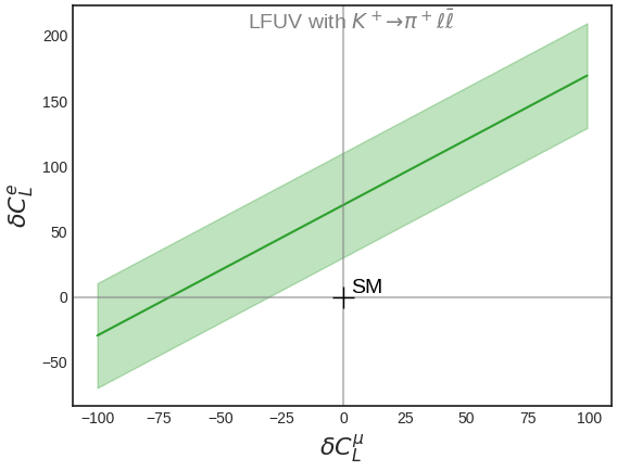
Figure 2: Region consistent with the estimation of the LFUV variable in $K^{+}\to\pi^{+}\ell\bar{\ell}$ decays.

2.3 BR($K_{S,L}\to\mu\bar{\mu}$), their interference and theoretical errors

The branching ratio of the $K_{S,L}\to\mu\bar{\mu}$ decays are interesting in different aspects. The precise determination of $K_{L}\to\mu\bar{\mu}$ PDG2020 in addition to the ongoing efforts in $K_{S}\to\mu\bar{\mu}$ by LHCb LHCb:2020ycd prompt the inclusion of these decay modes in the observables of interest. The analytic form of the branching fractions, in the absence of right-handed and (pseudo)scalar operators, and suited to our notation is given by Isidori:2003ts ; Chobanova:2017rkj

$${\rm BR}(K_{S}\to\mu\bar{\mu}) =\tau_{S}\frac{f_{K}^{2}m_{K}^{3}\beta_{\mu}}{16\pi}\left\{\beta_{\mu}^{2}\left|N_{S}^{\rm LD}\right|^{2}+\left(\frac{2m_{\mu}}{m_{K}}\frac{G_{F}\alpha_{e}}{\sqrt{2}\pi}\right)^{2}{\rm Im}^{2}\left[-\lambda_{c}\frac{Y_{c}}{s_{W}^{2}}+\lambda_{t}C_{10}^{\ell}\right]\right\},$$ (11)

and for the branching ratio of the $K_{L}\to\mu\bar{\mu}$ decay we have

$${\rm BR}(K_{L}\to\mu\bar{\mu}) =\tau_{L}\frac{f_{K}^{2}m_{K}^{3}\beta_{\mu}}{16\pi}\left|N_{L}^{\rm LD}-\left(\frac{2m_{\mu}}{m_{K}}\frac{G_{F}\alpha_{e}}{\sqrt{2}\pi}\right){\rm Re}\!\left[-\lambda_{c}\frac{Y_{c}}{s_{W}^{2}}+\lambda_{t}C_{10}^{\ell}\right]\right|^{2},$$ (12)

where the short-distance SM contribution is given by $Y_{c}$ and $C_{10,{\rm SM}}^{\ell}=C_{10,{\rm SM}}={-Y(x_{t})}/{s_{W}^{2}}$ (see appendix D) and the long-distance contributions as extracted in Chobanova:2017rkj from Ecker:1991ru ; Isidori:2003ts ; DAmbrosio:2017klp ; Mescia:2006jd  (see also Quigg:1968zz ; Martin:1970ai ; Savage:1992ac ; DAmbrosio:1992zqm ; DAmbrosio:1996lam ; Valencia:1997xe ; DAmbrosio:1997eof ; Cirigliano:2011ny ):

$$N_{S}^{\rm LD} =(-2.65+1.14i)\times 10^{-11}\textrm{\,(GeV})^{-2}\,,$$ (13)

$$N_{L}^{\rm LD} =\pm\left[0.54(77)-3.95i\right]\times 10^{-11}\textrm{\,(GeV})^{-2}\,,$$ (14)

with $N_{L}^{\rm LD}$ having an unknown sign (see appendix E for further details). Our SM evaluation for $K_{S,L}\to\mu\bar{\mu}$ using the updated inputs with the corresponding uncertainties are given below:

$$\text{BR}(K_{S}\to\mu\bar{\mu})^{\rm SM} =(5.15\pm 1.50)\times 10^{-12}\,,$$ (15)

$$\text{BR}(K_{L}\to\mu\bar{\mu})^{\rm SM} =\begin{cases}{\rm LD}(+)\!:\;\left(6.82^{+0.77}_{-0.24}\pm 0.04\right)\times 10^{-9}\,,\\[4.0pt] {\rm LD}(-)\!:\;\left(8.04^{+1.46}_{-0.97}\pm 0.09\right)\times 10^{-9}\,.\end{cases}$$ (16)

The estimation for BR($K_{S}\to\mu\bar{\mu}$) is in perfect agreement with past literature Ecker:1991ru ; Isidori:2003ts ; Gorbahn:2006bm ; DAmbrosio:2017klp . The corresponding evaluation of $K_{L}\to\mu\bar{\mu}$ leads to ‘two’ SM predictions, each corresponding to a given sign of $N_{L}^{\rm LD}$. The point of interest is in the evaluation of the corresponding asymmetric error emerging mainly from the uncertainty in the long-distance contribution. The existing computations quote symmetric errors which leads to a 1$\sigma$ agreement for both signs of $N_{L}^{\rm LD}$ with the corresponding experimental measurement. In this work, we investigate the asymmetric uncertainty of the branching fraction.

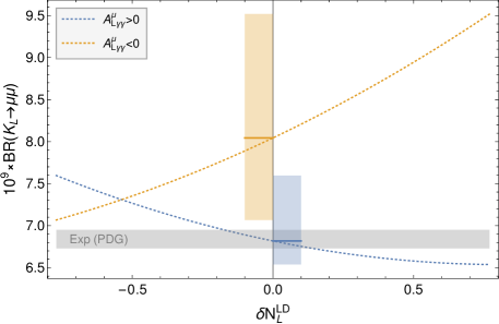
Figure 3: The SM theoretical error of BR($K_{L}\to\mu\bar{\mu}$) due to the uncertainty in the long-distance contribution.

The dotted lines in figure 3 show the variation in $K_{L}\to\mu\bar{\mu}$ as $N_{L}^{\rm LD}$ is varied over the 1$\sigma$ interval: blue (orange) corresponds to the +($-$) sign of $N_{L}^{\rm LD}$. The SM central values are represented by orange and blue horizontal lines in the coloured regions. The grey shaded region is the experimental measurement within the allowed $1\sigma$ error bars. Considering all inputs and assuming a Gaussian distribution of the errors of the inputs, we estimate the errors for each sign of $N_{L}^{\rm LD}$ with a Monte Carlo analysis (see appendix F for details). There are some points that stand out at this juncture: A) asymmetric pattern of the errors about the central values and B) minor disagreement (slightly above $1\sigma$) of the negative sign of $N_{L}^{\rm LD}$ with the experimental measurement.

The large uncertainty in the long-distance contribution results in quite asymmetric uncertainties in the branching ratio of $K_{L}\to\mu\bar{\mu}$ (see figure 3). The asymmetry is also reflected in the computation of $K_{L}\to\mu\bar{\mu}$ with the inclusion of NP. The left plot of figure 4 gives the computation of BR$(K_{L}\to\mu\bar{\mu})$ as a function of $\delta C_{L}^{\mu}(\equiv-\delta C_{10}^{\mu})$ for both signs of the long-distance contributions. The widths of the coloured bands represent the $1\sigma$ theoretical uncertainties. The band has a non-uniform width which appears to be pinched at $\delta C_{L}\simeq-5$ corresponding to the negligible lower uncertainty at that point. As noted before and in table 2, the experimental measurement of BR($K_{L}\to\mu\bar{\mu}$) is precise with less than 2% uncertainty and is shown by the grey band in the figure. Thus, irrespective of the large theory uncertainty and the unknown sign of the long-distance contributions from $A_{L\gamma\gamma}^{\mu}$, NP contribution to $\delta C_{L}^{\mu}$ is limited to the $[-13.4,3.4]$ range at 1$\sigma$.

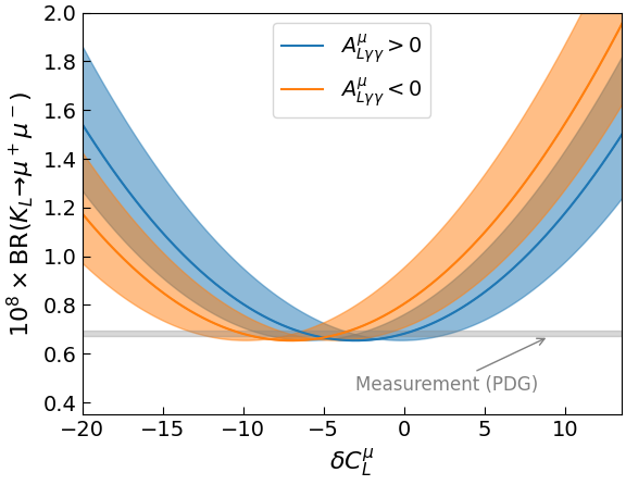
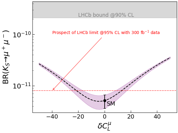
Figure 4: BR($K_{L}\to\mu\bar{\mu}$) as a function of $\delta C_{L}^{\mu}(\equiv\delta C_{9}^{\mu}=-\delta C_{10}^{\mu})$ assuming both possible signs for the long-distance contribution from $A_{L\gamma\gamma}^{\mu}$ on the left panel. BR($K_{S}\to\mu\bar{\mu}$) as a function of NP contributions in $\delta C_{L}^{\mu}$ on the right panel. In the left (right) panel, the grey band indicates the experimental measurement (upper limit) while the coloured bands correspond to the theoretical uncertainties. The LHCb bound and prospect for BR($K_{S}\to\mu\bar{\mu}$) are from ref. LHCb:2020ycd and ref. LHCb:2018roe , respectively.

The measurement of BR($K_{S}\to\mu\bar{\mu}$) is in its preliminary stages. This is illustrated by the right plot of figure 4, where the grey band gives the current upper bound from LHCb LHCb:2020ycd and the pink region gives the computation for a broad range of values of $\delta C_{L}$. The varying width corresponds to the varying uncertainty as a function of $\delta C_{L}$. Note that even with the projected reach of LHCb with an integrated luminosity of 300 fb^-1 of data, this decay mode on its own is not sensitive to the regions of $\delta C_{L}$ permitted by BR($K_{L}\to\mu\bar{\mu}$). This prompts us to include the interference effects with $K_{L}\to\mu\bar{\mu}$ in $K_{S}\to\mu\bar{\mu}$ which was proposed in DAmbrosio:2017klp (see also Dery:2021mct ). However, it should be noted that the future measurement of BR($K_{S}\to\mu\bar{\mu}$) at LHCb will be a powerful probe of New Physics scenarios involving scalar and pseudoscalar contributions Chobanova:2017rkj .

Figure 5 gives the impact of the interference of $K_{L}\to\mu\bar{\mu}$ on the effective branching fraction of $K_{S}\to\mu\bar{\mu}$. The results are presented for two extreme values of the dilution factor $D=\tfrac{K^{0}-\bar{K}^{0}}{K^{0}+\bar{K}^{0}}$, which is a measure of the initial asymmetry of $K^{0}$ and $\bar{K}^{0}$. The left (right) column corresponds to $A_{L\gamma\gamma}<0$ ($A_{L\gamma\gamma}>0$) and the shaded region in each plot represents the region ruled out by the measurement of BR($K_{L}\to\mu\bar{\mu}$). Comparing with figure 4, we note that the inclusion of interference effects makes the $\delta C_{L}^{\mu}\sim\mathcal{O}(1)$ region accessible to the high luminosity phase of LHCb.

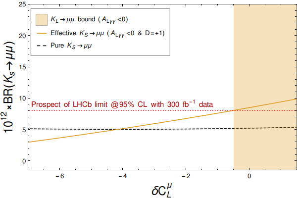
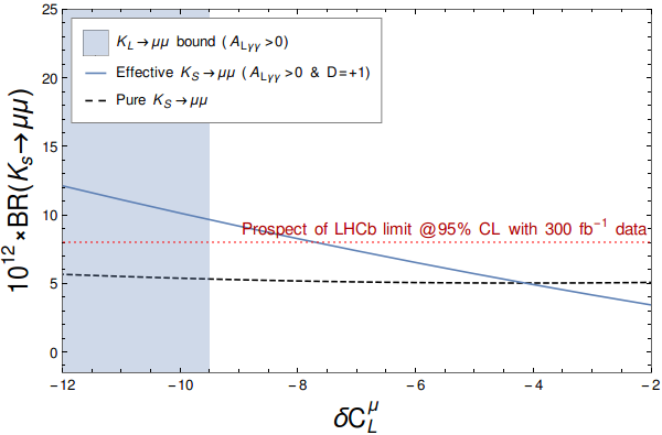
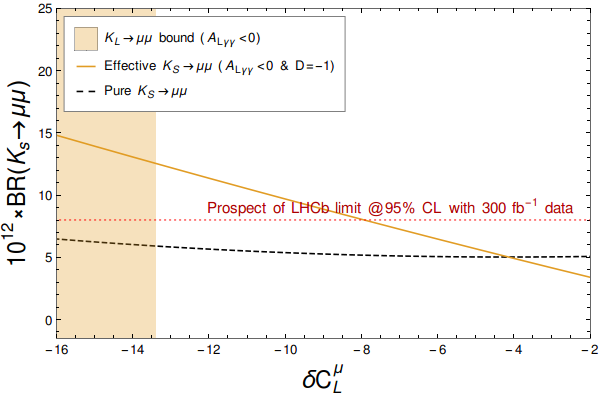
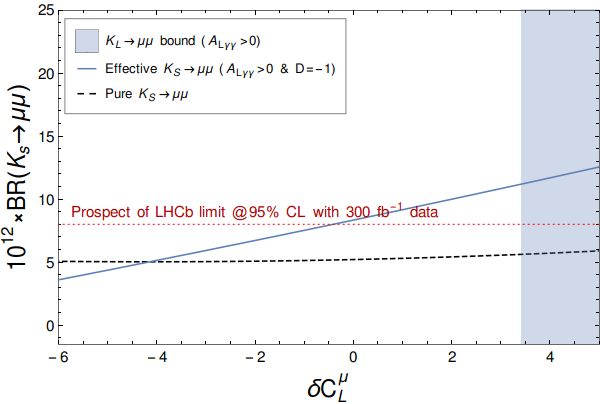
Figure 5: The impact of the interference of $K_{L}\to\mu\bar{\mu}$ on the effective branching fraction of $K_{S}\to\mu\bar{\mu}$. The left and the right panels correspond to negative and positive signs for $A_{L\gamma\gamma}$, respectively. The upper and lower panels correspond to dilution factor $D=+1$ and $D=-1$, respectively.

2.4 $K_{L}\to\pi^{0}\ell\bar{\ell}$

These processes have long been considered a smoking gun for the detection of direct CP violation. The description is composed of three contributions: the CP-conserving long-distance contribution, which is through the two-photon process $K_{L}\to\pi^{0}\gamma^{*}\gamma^{*}$, an indirect CP-violating contribution proportional to the CP-conserving process BR($K_{S}\to\pi^{0}\ell\bar{\ell}$) and $\epsilon$ which parameterises the $K^{0}-\bar{K}^{0}$ mixing and finally the direct CP-violating contribution. Considering the different contributions, the branching fraction of $K_{L}\to\pi^{0}\ell\bar{\ell}$ can be expressed as Buchalla:2003sj ; Isidori:2004rb ; Mescia:2006jd  (see also Martin:1970ai ; Ecker:1987qi ; Donoghue:1987awa ; Ecker:1987hd ; Ecker:1987fm ; Sehgal:1988ej ; Flynn:1988gy ; Cappiello:1988yg ; Morozumi:1988vy ; Ecker:1990in ; Savage:1992ac ; Cappiello:1992kk ; Heiliger:1992uh ; Cohen:1993ta ; Buras:1994qa ; DAmbrosio:1996kjn ; Donoghue:1997rr ; KTeV:1999gik ; Murakami:1999wi ; KTeV:2000amh ; Diwan:2001sg ; Gabbiani:2001zn ; Gabbiani:2002bk ; NA48:2002xke )

$${\rm BR}(K_{L}\to\pi^{0}\ell\bar{\ell})=\left(C_{\rm dir}^{\ell}\pm C_{\rm int}^{\ell}|a_{S}|+C_{\rm mix}^{\ell}|a_{S}|^{2}+C_{\gamma\gamma}^{\ell}\right)\cdot 10^{-12}\,,$$ (17)

with $|a_{S}|=1.20\pm 0.20$, extracted from experimental results on the branching fractions of $K_{S}\to\pi^{0}e\bar{e}$ and $K_{S}\to\pi^{0}\mu\bar{\mu}$. The numerical values of the different components are given in Mescia:2006jd as collected below:

	$C_{\rm dir}^{\ell}$	$C_{\rm int}^{\ell}$	$C_{\rm mix}^{\ell}$	$C_{\gamma\gamma}^{\ell}$
$\ell=e$	$(4.62\pm 0.24)(w_{7V}^{2}+w_{7A}^{2})$	$(11.3\pm 0.3)w_{7V}$	$14.5\pm 0.5$	$\approx 0$
$\ell=\mu$	$(1.09\pm 0.05)(w_{7V}^{2}+2.32w_{7A}^{2})$	$(2.63\pm 0.06)w_{7V}$	$3.36\pm 0.20$	$5.2\pm 1.6$

where $C_{\rm dir}$ corresponds to the direct CP-violating term determined by short-distance contributions proportional to Im($\lambda_{t}^{sd}$) in the SM (and minimal flavour violating scenarios Chivukula:1987fw ; Hall:1990ac ; Rattazzi:2000hs ; Buras:2000dm ; DAmbrosio:2002vsn ). The $C_{\rm mix}^{\ell}$ term indicates the indirect CP-violating contribution and $C_{\rm int}^{\ell}$ corresponds to the interference between the direct and indirect CP-violating contributions. The sign of the latter contribution is unclear, although constructive interference is preferred Buchalla:2003sj . Finally, the $C_{\gamma\gamma}^{\ell}$ ($\equiv C_{\rm CPC}$) term corresponds to the CP-conserving contribution from the two-photon intermediate states which can be deduced from the measurement of the $K_{L}\to\pi^{0}\gamma\gamma$ spectrum NA48:2002xke . The fact that this contribution is negligible for the electron mode strengthens the idea that the electron mode, in particular, could be an incontrovertible signal for the presence of direct CP violation. As indicated in Buchalla:2003sj , 40$\%$ of the contribution to the branching fraction is due to the clean short-distance physics, primarily driven by the interference with the indirect CP-violating part.

The $C^{\ell}_{\rm dir}$ and $C^{\ell}_{\rm int}$ contributions are parameterised by the factors $w_{7V,7A}$ which encode the short-distance SM and NP effects. They are defined as (see e.g. Bobeth:2016llm )

$$w_{7V}=\frac{1}{2\pi}{\rm Im}\left[\frac{\lambda_{t}^{sd}}{1.407\times 10^{-4}}C_{9}\right]\,,\quad w_{7A}=\frac{1}{2\pi}{\rm Im}\left[\frac{\lambda_{t}^{sd}}{1.407\times 10^{-4}}C_{10}\right]\,,$$ (18)

where $1.407\times 10^{-4}$ corresponds to the input used by Mescia:2006jd for $\lambda_{t}^{sd}$. Using the updated inputs in table 3 we find for constructive (destructive) interference

$${\rm BR}^{\rm SM}(K_{L}\to\pi^{0}e\bar{e}) =3.46^{+0.92}_{-0.80}\left(1.55^{+0.60}_{-0.48}\right)\times 10^{-11}\,,$$ (19)

$${\rm BR}^{\rm SM}(K_{L}\to\pi^{0}\mu\bar{\mu}) =1.38^{+0.27}_{-0.25}\left(0.94^{+0.21}_{-0.20}\right)\times 10^{-11}\,,$$ (20)

while current experimental bounds from KTeV KTeV:2003sls ; KTEV:2000ngj at 90% confidence level (CL) are one order of magnitude larger

$${\rm BR}^{\rm exp}(K_{L}\to\pi^{0}e\bar{e}) <28\times 10^{-11}\qquad\text{at 90\% CL}\,,$$ (21)

$${\rm BR}^{\rm exp}(K_{L}\to\pi^{0}\mu\bar{\mu}) <38\times 10^{-11}\qquad\text{at 90\% CL}\,.$$ (22)

It is expected that in the hybrid phase of the future CERN kaon program these decay modes are going to be observed Goudzovski:2022vbt . Currently, the dominating theoretical uncertainty is due to $|a_{S}|$ Buchalla:2008jp followed by the uncertainty on the two-photon intermediate state contribution in the muon mode which for destructive interference is as large as the uncertainty due to $|a_{S}|$. The prospect of the $|a_{S}|$ form factor determination is 10% statistical precision with LHCb Upgrade II LHCb:2018roe ; Alves:2018npj .

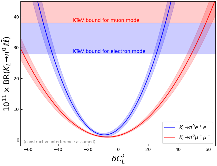
Figure 6: BR($K_{L}\to\pi^{0}\ell\bar{\ell}$) as a function of $\delta{C_{L}^{\ell}}(\equiv C_{9}^{\ell}=-C_{10}^{\ell})$ assuming constructive interference between direct and indirect CP-violating contributions.

The effect of NP in $\delta C_{L}$ on the branching fraction of $K_{L}\to\pi^{0}\ell\bar{\ell}$ is shown in figure 6 for the electron and the muon sectors. Since currently there are only upper bounds from experiments, these two observables do not put stringent constraints on possible NP contributions. For the muon sector, the upper bound gives a much weaker constrain compared to BR($K_{L}\to\mu\bar{\mu}$) as given in the previous subsection. Nonetheless, it is impressive that for the electron sector the current upper limit on BR($K_{L}\to\pi^{0}e\bar{e}$) which is about one order of magnitude larger than the SM prediction is already compatible with what is obtained by BR($K^{+}\to\pi^{+}\nu\bar{\nu}$), indicating $\delta C_{L}^{e}\lesssim 28$ at 90% CL.

3 Global picture

Table 2 summarises the results of the last section. The first column gives our evaluated SM value and the second column is the current experimental precision. The last column gives the experimental projection for the measurement of these observables and is detailed in section 3.1.

Observable	SM prediction	Exp results	Ref.	Experimental Err. Projections
BR$(K^{+}\to\pi^{+}\nu\nu)$	$(7.86\pm 0.61)\times 10^{-11}$	$(10.6^{+4.0}_{-3.5}\pm 0.9)\times 10^{-11}$	NA62:2021zjw	10%(@2025) 5%(CERN; long-term) Goudzovski:2022vbt
BR$(K^{0}_{L}\to\pi^{0}\nu\nu)$	$(2.68\pm 0.30)\times 10^{-11}$	$<3.0\times 10^{-9}$ @$90\%$ CL	Ahn:2018mvc	$20\%$(CERN; long-term  Goudzovski:2022vbt )  15% (KOTO NA62:2020upd )
LFUV($a_{+}^{\mu\mu}-a_{+}^{ee}$)	0	$-0.031\pm 0.017$	DAmbrosio:2018ytt ; Bician:2020ukv	$\pm 0.007$ (assuming $\pm 0.005$ for each mode)
BR$(K_{L}\to\mu\mu)$ ($+$)	$(6.82^{+0.77}_{-0.29})\times 10^{-9}$	$(6.84\pm 0.11)\times 10^{-9}$	PDG2020	experimental uncertainty kept to current value
BR$(K_{L}\to\mu\mu)$ ($-$)	$(8.04^{+1.47}_{-0.98})\times 10^{-9}$
BR$(K_{S}\to\mu\mu)$	$(5.15\pm 1.50)\times 10^{-12}$	$<2.1(2.4)\times 10^{-10}$ @$90(95)\%$ CL	LHCb:2020ycd	$<8\times 10^{-12}$ @$95\%$ CL (CERN; long-term LHCb:2018roe )
BR$(K_{L}\to\pi^{0}ee)(+)$	$(3.46^{+0.92}_{-0.80})\times 10^{-11}$	$<28\times 10^{-11}$ @$90\%$ CL	KTeV:2003sls	observation (CERN; long-term Goudzovski:2022vbt )
BR$(K_{L}\to\pi^{0}ee)(-)$	$(1.55^{+0.60}_{-0.48})\times 10^{-11}$
BR$(K_{L}\to\pi^{0}\mu\mu)(+)$	$(1.38^{+0.27}_{-0.25})\times 10^{-11}$	$<38\times 10^{-11}$ @$90\%$ CL	KTEV:2000ngj	(we assume 100% error)
BR$(K_{L}\to\pi^{0}\mu\mu)(-)$	$(0.94^{+0.21}_{-0.20})\times 10^{-11}$

Table 2: The SM predictions and experimental status for the different observables. The SM values and the corresponding uncertainties in the first column are evaluated using the updated inputs using SuperIso Mahmoudi:2008tp . In the second column, the current experimental status is given. The third column gives the projections in experimental sensitivity for the corresponding experiments (see also Goudzovski:2022 ). For the case with more than one projection, the CERN long-term ones are used.

It is convenient to present a unified picture of the topics discussed thus far.

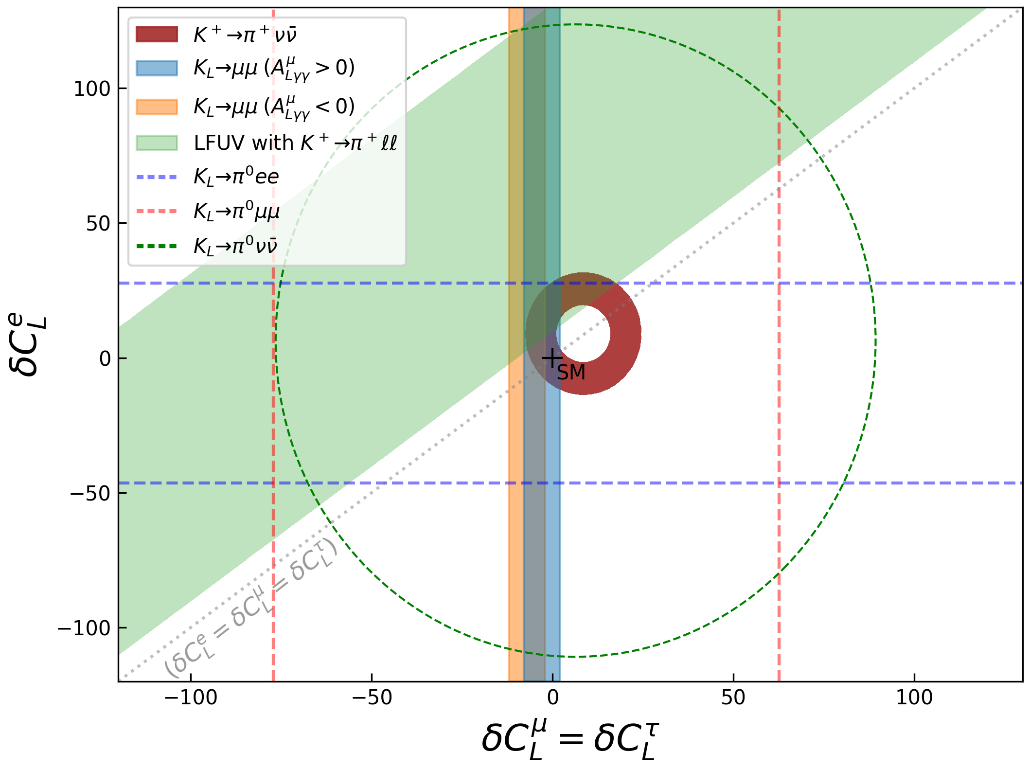
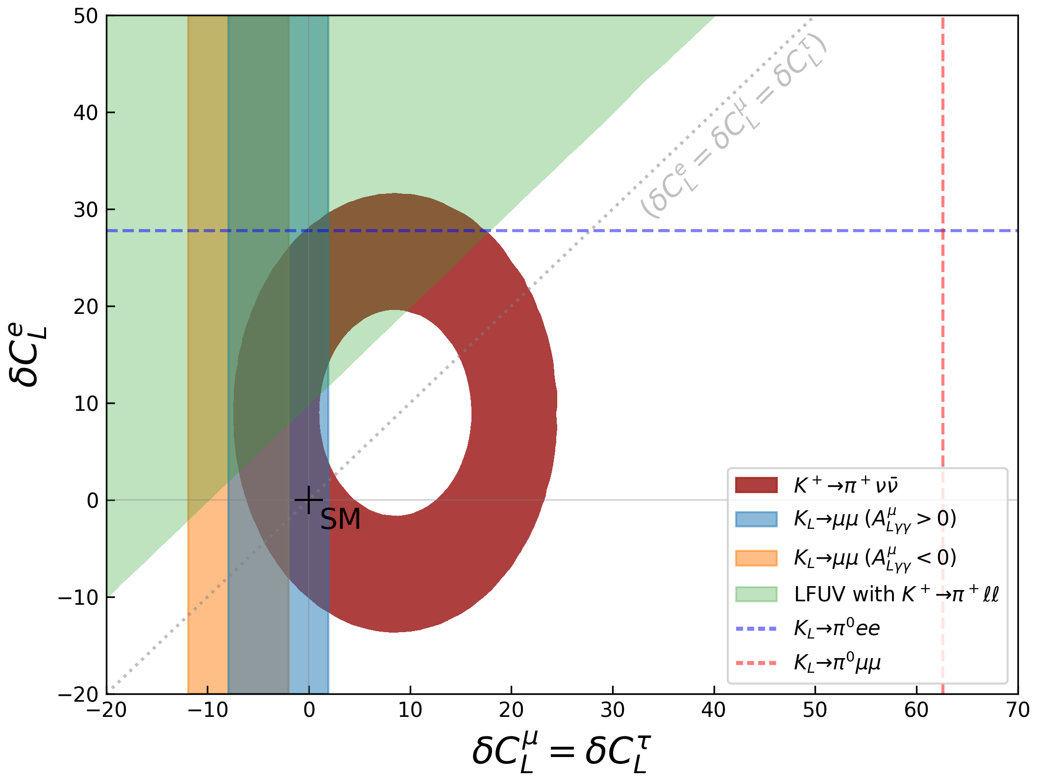
Figure 7: The bounds from individual observables. The right panel is the zoomed version of the left panel. The coloured regions correspond to $68\%$ CL when there is a measurement and the dashed ones to upper limits at 90% CL. $K_{L}\to\mu\bar{\mu}$ has been shown for both signs of the long-distance contribution. For $K_{L}\to\pi^{0}e\bar{e}$ and $K_{L}\to\pi^{0}\mu\bar{\mu}$, constructive interference between direct and indirect CP-violating contributions has been assumed.

In figure 7, for each individual observable, we show the $68\%$ CL regions in the $(\delta C_{L}^{e},\delta C_{L}^{\mu})$ plane for those observables which have been measured, as well as the 90% CL upper limits for the observables where there are only upper bounds. Note the mild tension in the upper part of the 68% CL region of $K^{+}\to\pi^{+}\nu\bar{\nu}$ (in maroon) with the upper bound on $K_{L}\to\pi^{0}e\bar{e}$ (dashed blue line). This is specific to the case where we choose $\delta C_{L}^{\mu}=\delta C_{L}^{\tau}$. A contrasting picture corresponding to $\delta C_{L}^{e}=\delta C_{L}^{\tau}$ is presented in figure 12 in appendix C.

A zoomed version is shown in the right plot. Other decays include $K_{L}\to\mu\bar{\mu}$ shown with the orange (blue) band for negative (positive) long-distance contributions. The upper bound from $K_{L}\to\pi^{0}\nu\bar{\nu}$ is indicated by the dashed green line. The region of intersection by the horizontal blue dashed and the vertical red dashed lines represent the parameter space allowed by $K_{L}\to\pi^{0}\ell\bar{\ell}$. While this is instructive, it would be useful to find the region in the $(\delta C_{L}^{\mu}=\delta C_{L}^{\tau},\,\delta C_{L}^{e})$ plane which is consistent with all observables. This prompts the implementation of a global fit, similar to those employed for $B$ decays. However, given the limited experimental data for most observables, we adapt a multi-prong strategy for the fits taking into account both the current and future possibilities for many of these observables.

3.1 Global fits

We begin with the definition of the $\chi^{2}$ statistic as follows:

$$\chi^{2}=\sum_{i,j=1}^{N}\left(O_{i}^{\rm th}(\delta C_{L}^{e,\mu})-O_{i}^{\rm exp}\right)\;C_{ij}^{-1}\;\left(O_{j}^{\rm th}(\delta C_{L}^{e,\mu})-O_{j}^{\rm exp}\right)\,,$$ (23)

where $C_{i,j}$ denotes the total (theoretical and experimental) covariance matrix. Note that an observable ${O}_{i}^{\rm th}$ in eq. 23 is expressed as a function of $\delta C_{L}^{e,\mu}$, and the contribution due to $\delta C_{L}^{\tau}$ is in principle not fixed in a two-dimensional fit to $\delta C_{L}^{e,\mu}$. Henceforth, unless otherwise stated we stick to the convention $\delta C_{L}^{\tau}=\delta C_{L}^{\mu}$. While this choice is motivated by the convention followed in the paper thus far, the future phase of data accumulation for each of these experiments would enable us to make a more adequate choice. To ensure clarity, we divide the discussion that follows into two parts: fits with current data and projected fits.

3.2 Fits with current data

We first perform a New Physics fit of $\delta C_{L}^{e}$ and $\delta C_{L}^{\mu}=\delta C_{L}^{\tau}$ to the current experimental data on rare kaon decays (collected in the second column of table 2). The results of the fit are given in figure 8 where the 68 and 95% CL regions are given in light and dark purple, respectively. Due to the ambiguity in the sign of the long-distance contribution from $A_{L\gamma\gamma}$ to $K_{L}\to\mu\bar{\mu}$, the fit results are given for both signs with $A_{L\gamma\gamma}<0\;(>0)$ on the left (right). The purple cross in each plot represents the corresponding best-fit point. While the fits are qualitatively similar, we note the appearance of a wall-shaped feature on the left side of the fit for $A_{L\gamma\gamma}>0$ (right), which is better defined than the one corresponding to $A_{L\gamma\gamma}<0$ (left). Its origin can be traced back to the blue band in figure 7. But in general, the difference in shapes for the fits between positive and negative values of $A_{L\gamma\gamma}$ show that a future improvement in the sensitivity can lead to a resolution of the sign ambiguity.

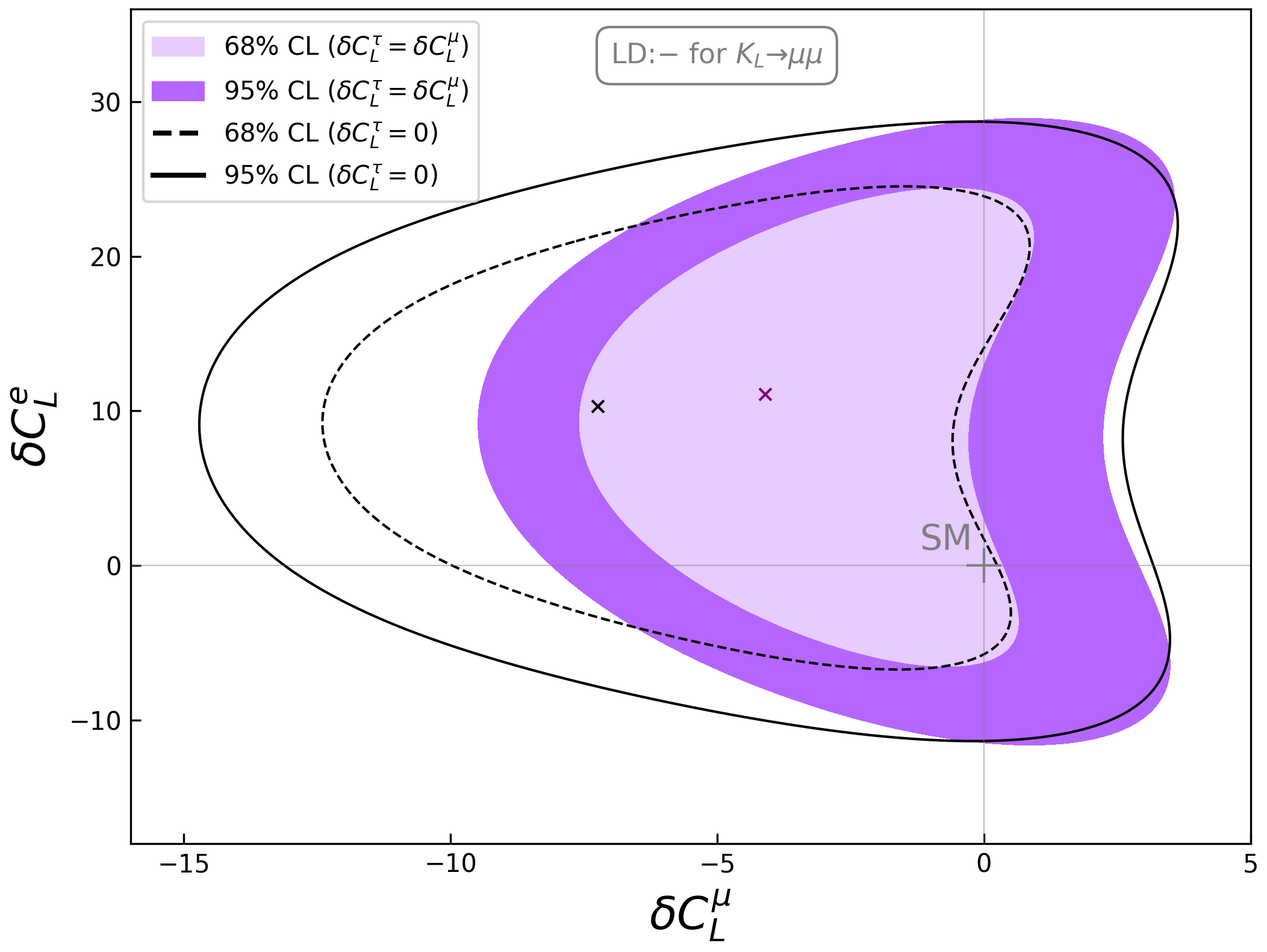
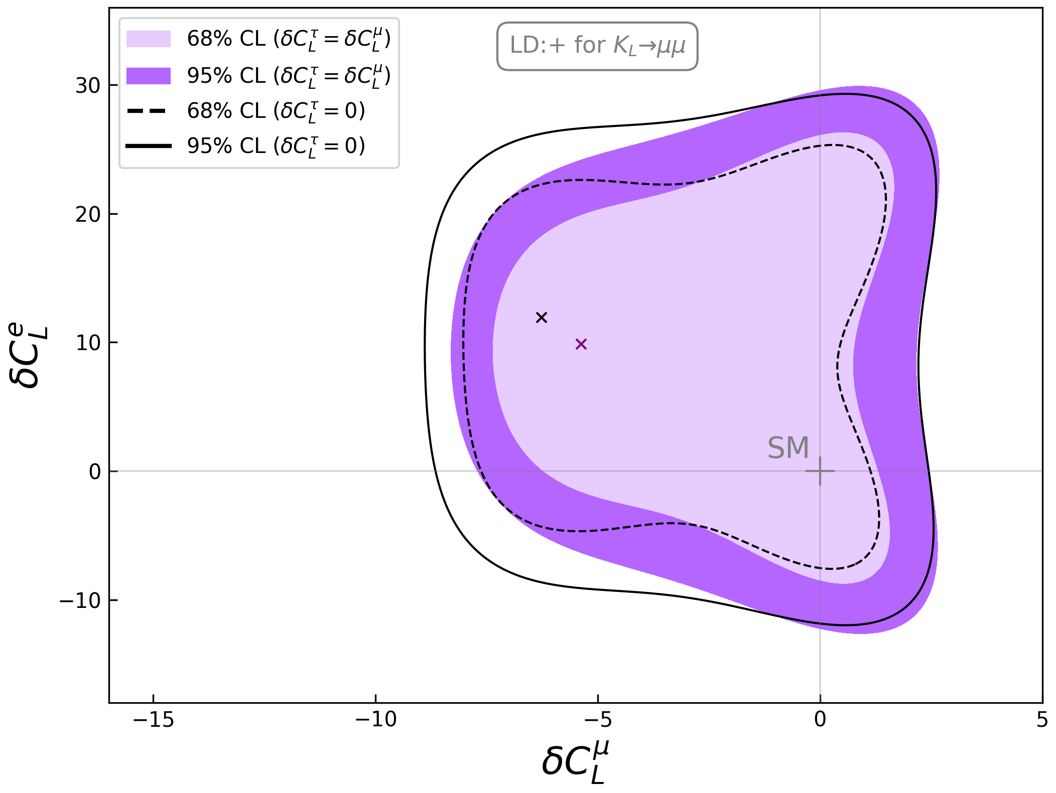
Figure 8: Comparison of the global fits between scenarios $\delta C_{L}^{\tau}=\delta C_{L}^{\mu}$ (purple regions) and $\delta C_{L}^{\tau}=~{}\!\!0$ (black solid and dashed lines). The fits are implemented using existing data with long-distance contribution to $K_{L}\to\mu\bar{\mu}$ having a negative (positive) sign, on the left (right).

One of the defining features of kaon decays is that it allows a “relatively clean” possibility for identifying the extent of contributions due to effective operators involving tau leptons. Note that the “relatively clean” refers to both the status of the SM computation as well as the future projections for the measurement of observables where operators involving the tau leptons play a direct role. These operators contribute to the computation of $K^{+}\to\pi^{+}\nu\bar{\nu}$ and $K_{L}\to\pi^{0}\nu\bar{\nu}$. As explained in detail in section 2, both are characterised by highly precise SM computations, owing to negligible long-distance uncertainties. Furthermore, there exists a well-defined strategy for a highly precise measurement of both decays Goudzovski:2022 ; NA62:2021zjw ; Ahn:2018mvc . It is natural to expect insight into the extent of the contributions due to the operators involving tau leptons by means of global analyses which include these decay modes. This can be illustrated by a comparison of the fits in the absence of $\delta C_{L}^{\tau}$ as shown with dashed and solid black lines corresponding to the 68 and 95% CL regions, respectively. The black cross in figure 8 indicates the best-fit point for the case of $\delta C_{L}^{\tau}=0$. A feature common to both signs of $A_{L\gamma\gamma}$ is that the $\delta C_{L}^{\tau}=\delta C_{L}^{\mu}$ case prefers a smaller parameter space, translating into a strong lower bound on $\delta C_{L}^{\mu}$. The larger spread in $\delta C_{L}^{\mu}$ for the fit with $\delta C_{L}^{\tau}=0$ can be attributed to the larger contribution required from the same to be consistent with the observation of $K^{+}\to\pi^{+}\nu\bar{\nu}$. Other noticeable feature is the shapes of the 68$\%$ CL contours on the right for both plots. The depression in the centre can be attributed to the region allowed by $K^{+}\to\pi^{+}\nu\bar{\nu}$ shown in maroon in figure 7. Furthermore, the wall-like feature on the left side of the global fit on the right plot reflects the region allowed by $K_{L}\to\mu\bar{\mu}$ and shown by the blue band in figure 7.

Visually, the left plot reveals a greater level of discrimination between the two scenarios. This is because of a relatively stronger lower bound on $\delta C^{\mu}_{L}$ for the negative sign of $A_{L\gamma\gamma}$ as shown by the orange region in figure 7. However, for either plot, the two scenarios are statistically equivalent with the present data. A concrete discrimination may be possible with future runs of many of these experiments. This information would be available by $\sim 2035$, at the projected end of data accumulation for NA62/KOTO thereby reaching the required precision. This strengthens the possibility of kaon experiments offering a handle on effective operators involving tau.

3.3 Projection fits

The results of the above fit arouse a natural curiosity about the possible impact of the future runs of the experiments. Given the preliminary stage of the run of most of these experiments, any projection on the fits requires both the possible measured value as well as the experimental precision. The latter is rather straightforward and we can adapt the intended long-term experimental precision that is true for some of the decay modes. In the case of $K^{+}(K_{L})\to\pi^{+}(\pi^{0})\nu\bar{\nu}$, there is a well-defined sensitivity goal due to NA62/KOTO. In the case of LFUV in $K^{+}\to\pi^{+}\ell\bar{\ell}$, we assume the uncertainty on $a_{+}^{\ell\ell}$ to become less than half the current value to reach $0.005$ for either of the electron and muon modes. For $K_{L}\to\pi^{0}\ell\bar{\ell}$ as mentioned in section 2.4 they are expected to be observed in the future CERN kaon program, however, in the absence of a well-defined projection for the uncertainty, we assume 100$\%$ error. All the numbers are collected in the last column of table 2. A prediction of the possible measured central value, on the other hand, is not possible, especially for those with only an existing upper bound. In light of this, we present a two-faceted approach. In the first approach, labelled projection A, the predicted central values for those observables with only an upper bound is projected to be the same as the SM prediction. On the other hand, the corresponding values for $K^{+}\to\pi^{+}\nu\bar{\nu}$, LFUV in $K^{+}\to\pi^{+}\ell\bar{\ell}$ and $K_{L}\to\mu\bar{\mu}$ are chosen to be the same as the existing measurement. In the second approach, labelled projection B, the central values for all of the observables are projected with the best-fit points obtained from the fits with the existing data.

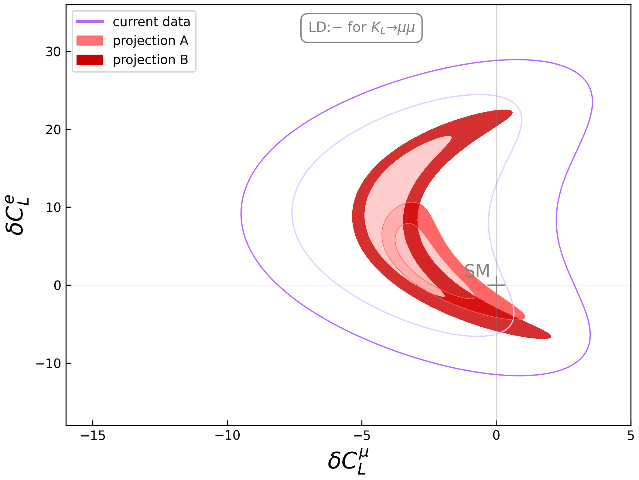
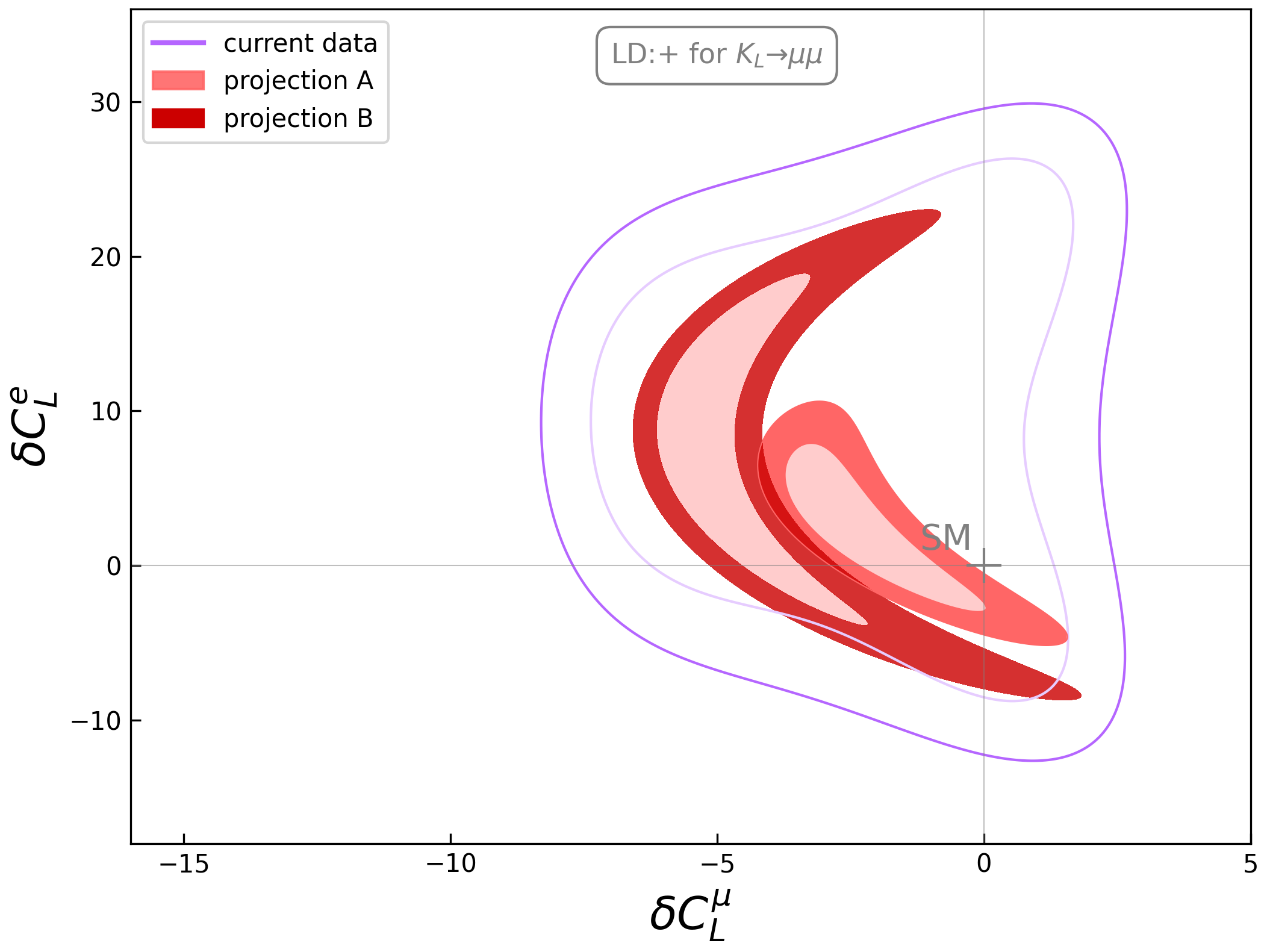
Figure 9: Projected fit to rare kaon observables within 68 and 95% CL assuming negative (positive) sign for the long-distance contribution to $K_{L}\to\mu\bar{\mu}$ on the left (right). Lighter shades of red: projection A with central values from current measurements (whenever there is one) or SM predictions (if currently not observed). Darker shades of red: projection B with current best-fit point used for all projections. The contours of the fit to current data (corresponding to the purple regions in figure 8) are shown with purple solid lines.

The results of the fits, for projections A and B, are illustrated in figure 9 with ${A_{L\gamma\gamma}<0\;(>)}$ on the left (right). The 68 and 95% CL regions are shown with lighter shades of red for projection A and similarly for projection B with darker shades of red. A comparison with fit to current data as indicated by the purple solid contours (coinciding with the 68 and 95% contours of the purple regions in figure 8) reveals a significant reduction in the parameter space for both projections. Projection A leads to an overall consistency with the SM, represented by $(0,0)$, up to $3\sigma$. This can be expected with the choice of the predicted central values being the same as the SM for those observables not currently measured. Projection B on the other hand predicts an overwhelming departure from the SM. This is also in line with our expectation as the best-fit points of the fits to the current data (purple crosses in figure 8) presented a significant departure from their corresponding SM prediction with the assumption of the projected sensitivities.

The entire discussion of section 3 can be conveniently encapsulated by presenting a summary plot in figure 10. The left (right) plot corresponds to $A_{L\gamma\gamma}<0~{}(>0)$. Either plot gives the results with the current fit along with the two approaches for the projected global fits: projection A (lighter shade of red) and B (darker shade of red). They are overlaid on the results of figure 7. This gives us an illustrative understanding of the observables that are the driving force behind the fits. As expected, $K^{+}\to\pi^{+}\nu\bar{\nu}$, shown by the “maroon-doughnut” shape plays the most significant role in determining the shape of the regions. This is true for both the current as well as the projected fits. In an ideal case, one would expect the regions to be concentrated towards the top left for the projected fit due to the impact of the LFUV observables. However, the dominance of the theoretical errors due to $K_{L}\to\mu\bar{\mu}$ makes its effect to be less pronounced.

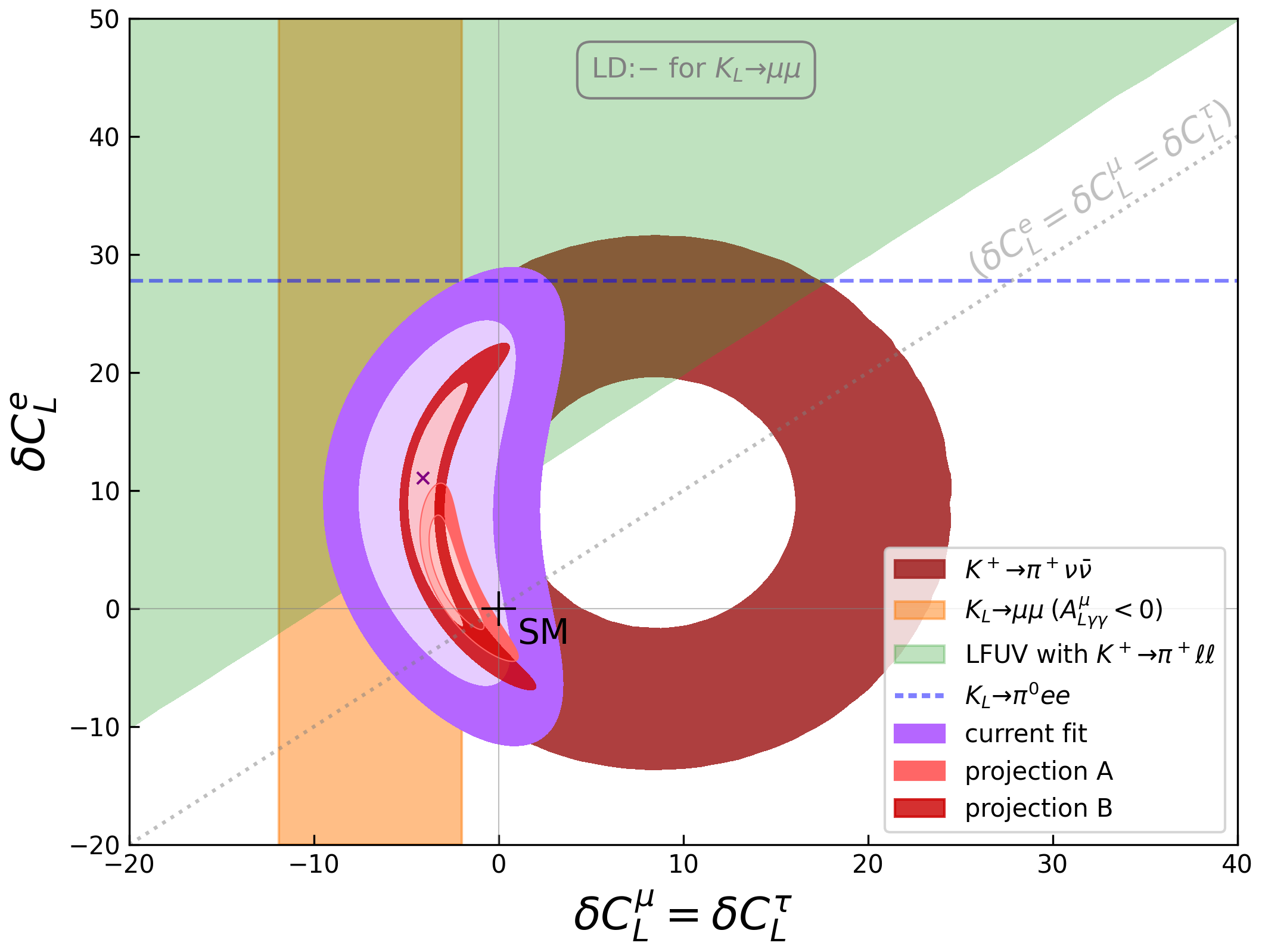
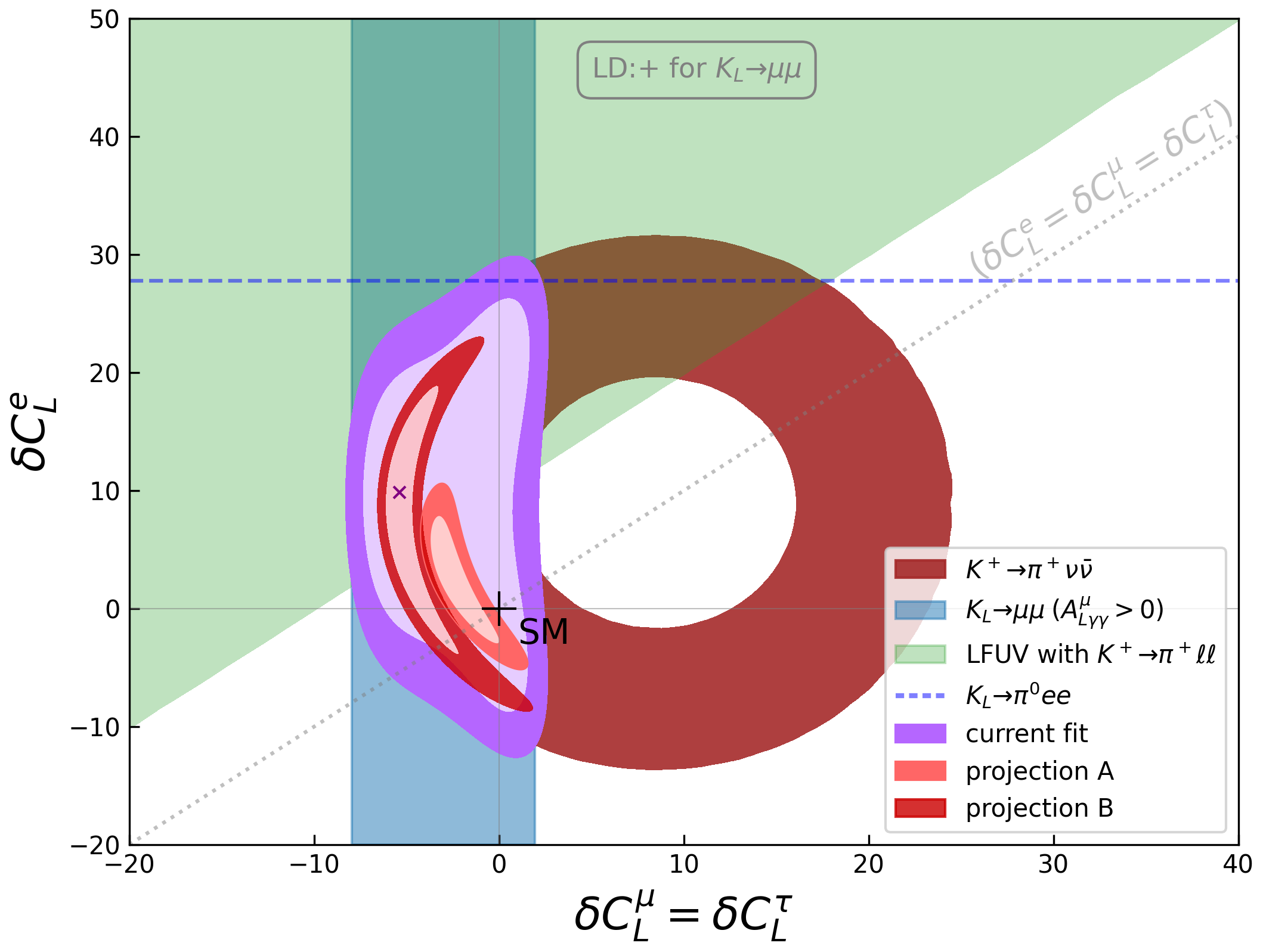
Figure 10: Global fit with current data (in purple) and projection A (lighter shades of red) and projection B (darker shades of red) together with 68% CL for individual observables with current data. The purple cross indicates the best-fit point with the current data.

4 Conclusions

This work, motivated by $B$-anomalies, presents a possible new way to analyse rare kaon decays looking for LFUV: we have performed global fits to the Wilson coefficients of the operators contributing to kaon decays. The road leading to the fits is set up by a careful re-examination of the different observables involved. This includes a computation of the SM values and the theoretical uncertainties. In the case of the latter, asymmetric uncertainties were observed for some of the modes, in particular for $K_{L}\to\mu\bar{\mu}$. These inputs were then used to construct a global picture and develop a strategy for the fits, which were divided into two parts. The first part gave a glimpse into the existing parameter space using the current experimental information. This was then followed by a “projection-fit” which took into account the future sensitivity and measurement goals for many of the observables while assuming realistic projections for the rest (e.g. vector form factors in $K^{+}\to\pi^{+}\ell\bar{\ell}$). Given the uncertainty in the experimental central values for the observables for which only an upper bound exists, we adapted two methodologies: A) assuming SM as the central values and B) assuming the best-fit values from the existing fits as the central values. The results of the projection-fit highlighted the need to achieve a better accuracy in the theoretical computation of $K_{L}\to\mu\bar{\mu}$. Our $K_{L}\to\mu\bar{\mu}$ analysis leading to asymmetric errors indicates quantitatively how to strategically improve the theoretical error in order to solve the ambiguity in the sign of the long-distance contributions (can be resolved if there is an improvement by about $\sim 50\%$). Although not considered in our global fit, we also demonstrated the interference of $K_{S}\to\mu\bar{\mu}$ and $K_{L}\to\mu\bar{\mu}$ besides giving a handle on the sign of the SM long-distance contributions in the latter, can be an effective probe of NP in the muon sector (in case of having an experimental setup with a large dilution factor). This analysis presented a global picture of the physics goals that can be achieved with kaon experiments, and the possibility to probe sensitivity to lepton flavour universality violating New Physics.

Appendix A Input parameters

Table 3 gives the input values used in the computation of different observables.

$m_{K^{\pm}}=493.677(16)$ MeV	PDG2020	$\lambda=0.22650(48)$	PDG2020
$m_{K}=497.611(13)$ MeV	PDG2020	$A=0.790(17)$	PDG2020
$m_{c}(m_{c})=1.27(2)$ GeV	PDG2020	$\bar{\rho}=0.141(17)$	PDG2020
$m_{b}(m_{b})=4.18^{+0.03}_{-0.02}$ GeV	PDG2020	$\bar{\eta}=0.357(11)$	PDG2020
$m_{t}^{pole}=172.69(30)$ GeV	PDG2020	$\lambda_{t}^{sd}=\left[-3.11(15)+i\,1.36(7)\right]\times 10^{-4}$
$f_{K}=155.7(3)$ MeV	FlavourLatticeAveragingGroup:2019iem

Table 3: Input parameters used in this work.

Appendix B $X(x_{t})$ and $X_{c}$ expressions

The short-distance contribution $X(x_{t})$ in the SM (extracted from the original papers Buchalla:1993bv ; Misiak:1999yg ; Buchalla:1998ba ; Brod:2010hi ) is given in Buras:2015qea

$$X(x_{t})=X_{0}(x_{t})+\frac{\alpha_{s}(\mu_{t})}{4\pi}X_{1}(x_{t})+\frac{\alpha}{4\pi}X_{\rm EW}(x_{t}),$$ (24)

where $X_{0}$ is the leading order result, and $X_{1}$, $X_{\rm EW}$ are the NLO QCD and EW corrections, respectively. The coupling constants $\alpha_{s}$ and $\alpha$, as well as the parameter $x_{t}=m_{t}^{2}/m_{W}^{2}$, have to be evaluated at scale $\mu\sim\mathcal{O}(M_{t})$. The LO expression is the gauge-independent linear combination $X_{0}(x_{t})\equiv C(x_{t})-4B(x_{t})$ Inami:1980fz ; Buchalla:1990qz

$$X_{0}(x_{t})=\frac{x_{t}}{8}\left[\frac{x_{t}+2}{x_{t}-1}+\frac{3x_{t}-6}{(x_{t}-1)^{2}}\log x_{t}\right].$$ (25)

The NLO QCD correction Buchalla:1993bv ; Misiak:1999yg ; Buchalla:1998ba , in the $\overline{\text{MS}}$ scheme reads

$$X_{1}(x_{t}) =-\frac{29x_{t}-x_{t}^{2}-4x_{t}^{3}}{3(1-x_{t})^{2}}-\frac{x_{t}+9x_{t}^{2}-x_{t}^{3}-x_{t}^{4}}{(1-x_{t})^{3}}\log x_{t}$$ (26)

$$+\frac{8x_{t}+4x_{t}^{2}+x_{t}^{3}-x_{t}^{4}}{2(1-x_{t})^{3}}\log^{2}x_{t}-\frac{4x_{t}-x_{t}^{3}}{(1-x_{t})^{2}}{\rm Li}_{2}(1-x_{t})$$

$$+8x_{t}\frac{\partial X_{0}}{\partial x_{t}}\log\frac{\mu^{2}}{M_{W}^{2}},$$

where $\mu$ is the renormalisation scale. The 2-loop EW correction $X_{\rm EW}$ has been calculated in Brod:2010hi . The charm contributions, $X_{c}^{\nu}(\equiv\lambda^{4}P_{c}(X))$, are described via

$$P_{c}(X)=P_{c}^{\rm SD}(X)+\delta P_{c,u}$$ (27)

where $\delta P_{c,u}=0.04\pm 0.02$ corresponds to the long-distance contributions as calculated in ref. Isidori:2003ts . The short-distance contribution of the charm quark $P_{c}(X)$ including NNLO correction is calculated in ref. Brod:2008ss but the explicit analytical expression is not given. However, an approximate formula is given by

$$\begin{split}P_{c}^{\rm SD}(X)&=0.38049\left(\frac{m_{c}(m_{c})}{1.30\textrm{GeV}}\right)^{0.5081}\left(\frac{\alpha_{s}(M_{Z})}{0.1176}\right)^{1.0192}\left(1+\sum_{i,j}\kappa_{ij}L_{m_{c}}^{i}L_{\alpha_{s}}^{j}\right)\\ &\pm 0.008707\left(\frac{m_{c}(m_{c})}{1.30\textrm{GeV}}\right)^{0.5276}\left(\frac{\alpha_{s}(M_{Z})}{0.1176}\right)^{1.8970}\left(1+\sum_{i,j}\epsilon_{ij}L_{m_{c}}^{i}L_{\alpha_{s}}^{j}\right)\,,\end{split}$$ (28)

where

$$L_{m_{c}}=\ln\left(\frac{m_{c}(m_{c})}{1.30\textrm{GeV}}\right)\,,\qquad L_{\alpha_{s}}=\ln\left(\frac{\alpha_{s}(M_{Z})}{0.1176}\right)\,,$$ (29)

and

$$\kappa_{10}=1.6624,\quad\kappa_{01}=-2.3537,\quad\kappa_{11}=-1.5862,\quad\kappa_{20}=1.5036,\quad\kappa_{02}=-4.3477,$$

$$\epsilon_{10}=-0.3537,\quad\epsilon_{01}=0.6003,\quad\epsilon_{11}=-4.7652,\quad\epsilon_{20}=1.0253,\quad\epsilon_{02}=0.8866.$$ (30)

The NP effects that are neutrino-flavour dependent, beside NP$\times$NP terms contribute via SM$\times$NP interference terms. Thus, for these types of NP effects in ${\rm BR}(K^{+}\to\pi^{+}\nu\bar{\nu})$ we need the NNLO charm contributions for the different neutrino flavours in a separated form (see eq. 33 below). However, since the charm contributions are not available separately at NNLO as given in eq. 28, for the SM$\times$NP interference terms we use the NLO results from appendix C.2 of ref. Bobeth:2016llm which is given for $\mu_{c}=1.3$ GeV

$$X_{c}^{e/\mu} =10.05\times 10^{-4}, X_{c}^{\tau}=6.64\times 10^{-4}.$$ (31)

The SM$\times$NP interference terms are clearly seen when having eqs. 4 and 5 in their expanded form

$${\rm BR}(K_{L}\to\pi^{0}\nu\bar{\nu})=\frac{\kappa_{L}}{\lambda^{10}}\frac{1}{3}s_{W}^{4}\sum_{\nu_{\ell}}{\rm Im}^{2}\left[\lambda_{t}C_{L}^{\nu_{\ell}}\right]$$ (32)

$$={\rm BR}(K_{L}\to\pi^{0}\nu\bar{\nu})_{\rm SM}+\frac{\kappa_{L}}{\lambda^{10}}\frac{1}{3}s_{W}^{4}\Bigg{[}\sum_{\nu_{\ell}}\mbox{Im}^{2}\left(\lambda_{t}\,C_{L,{\rm NP}}^{\nu_{\ell}}\right)+2\,\mbox{Im}\left(\lambda_{t}\,C_{L,{\rm SM}}\right)\sum_{\nu_{\ell}}\mbox{Im}\left(\lambda_{t}\,C_{L,{\rm NP}}^{\nu_{\ell}}\right)\Bigg{]}$$

$${\rm BR}(K^{+}\to\pi^{+}\nu\bar{\nu})=\frac{\kappa_{+}(1+\Delta_{\rm EM})}{\lambda^{10}}\frac{1}{3}s_{W}^{4}\sum_{\nu_{\ell}}\left[{\rm Im}^{2}\Big{(}\lambda_{t}C_{L}^{\nu_{\ell}}\Big{)}+{\rm Re}^{2}\Big{(}-\frac{\lambda_{c}X_{c}}{s_{W}^{2}}+\lambda_{t}C_{L}^{\nu_{\ell}}\Big{)}\right]$$ (33)

$$={\rm BR}(K^{+}\to\pi^{+}\nu\bar{\nu})_{\rm SM}+\frac{\kappa_{+}(1+\Delta_{\rm EM})}{\lambda^{10}}\frac{1}{3}s_{W}^{4}\Bigg{[}\sum_{\nu_{\ell}}\mbox{Im}^{2}\left(\lambda_{t}C_{L,{\rm NP}}^{\nu_{\ell}}\right)+2\,\mbox{Im}\left(\lambda_{t}C_{L,{\rm SM}}\right)\sum_{\nu_{\ell}}\mbox{Im}\left(\lambda_{t}C_{L,{\rm NP}}^{\nu_{\ell}}\right)$$

$$\quad+\sum_{\nu_{\ell}}\mbox{Re}^{2}\left(\lambda_{t}C_{L,{\rm NP}}^{\nu_{\ell}}\right)+2\,\mbox{Re}\left(\lambda_{t}C_{L,{\rm SM}}\right)\sum_{\nu_{\ell}}\mbox{Re}\left(\lambda_{t}C_{L,{\rm NP}}^{\nu_{\ell}}\right)-2\sum_{\nu_{\ell}}\mbox{Re}\left(\frac{\lambda_{c}X_{c}^{\nu}}{s_{W}^{2}}\right)\mbox{Re}\left(\lambda_{t}C_{L,{\rm NP}}^{\nu_{\ell}}\right)\Bigg{]}$$

Appendix C Results with $\delta C_{L}^{e}=\delta C_{L}^{\tau}$

In this section, we provide the results of the scan corresponding to the possibility where the NP Wilson coefficients for the electron and tau are set equal to each other: $\delta C_{L}^{e}=\delta C_{L}^{\tau}$. As tau contribution is relevant only for the decays involving the neutrinos, we present the other possibility for figures 1 and 7.

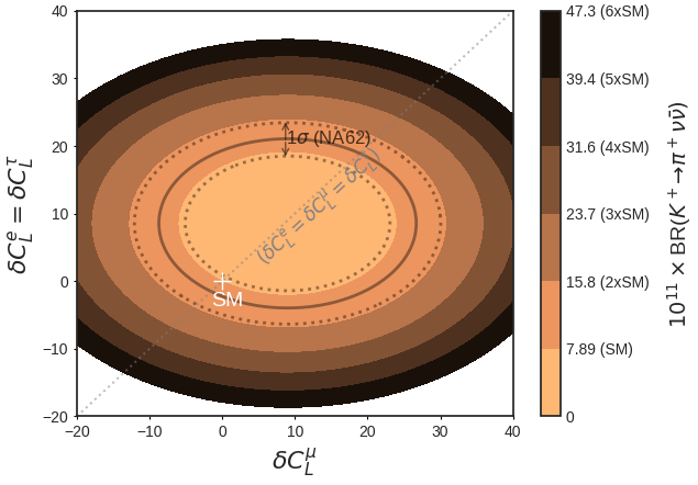
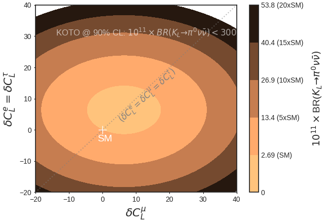
Figure 11: BR($K^{+}\to\pi^{+}\nu\bar{\nu}$) (left) and BR($K_{L}\to\pi^{0}\nu\bar{\nu}$) (right) as a function of $\delta C_{L}^{e}=\delta C_{L}^{\tau}$ and $\delta C_{L}^{\mu}$. In the left plot, the solid (dashed) line corresponds to the measured central value ($1\sigma$ experimental uncertainty) by NA62 NA62:2021zjw . In the right the upper bound on BR($K_{L}\to\pi^{0}\nu\bar{\nu}$) is not visible for the values scanned.

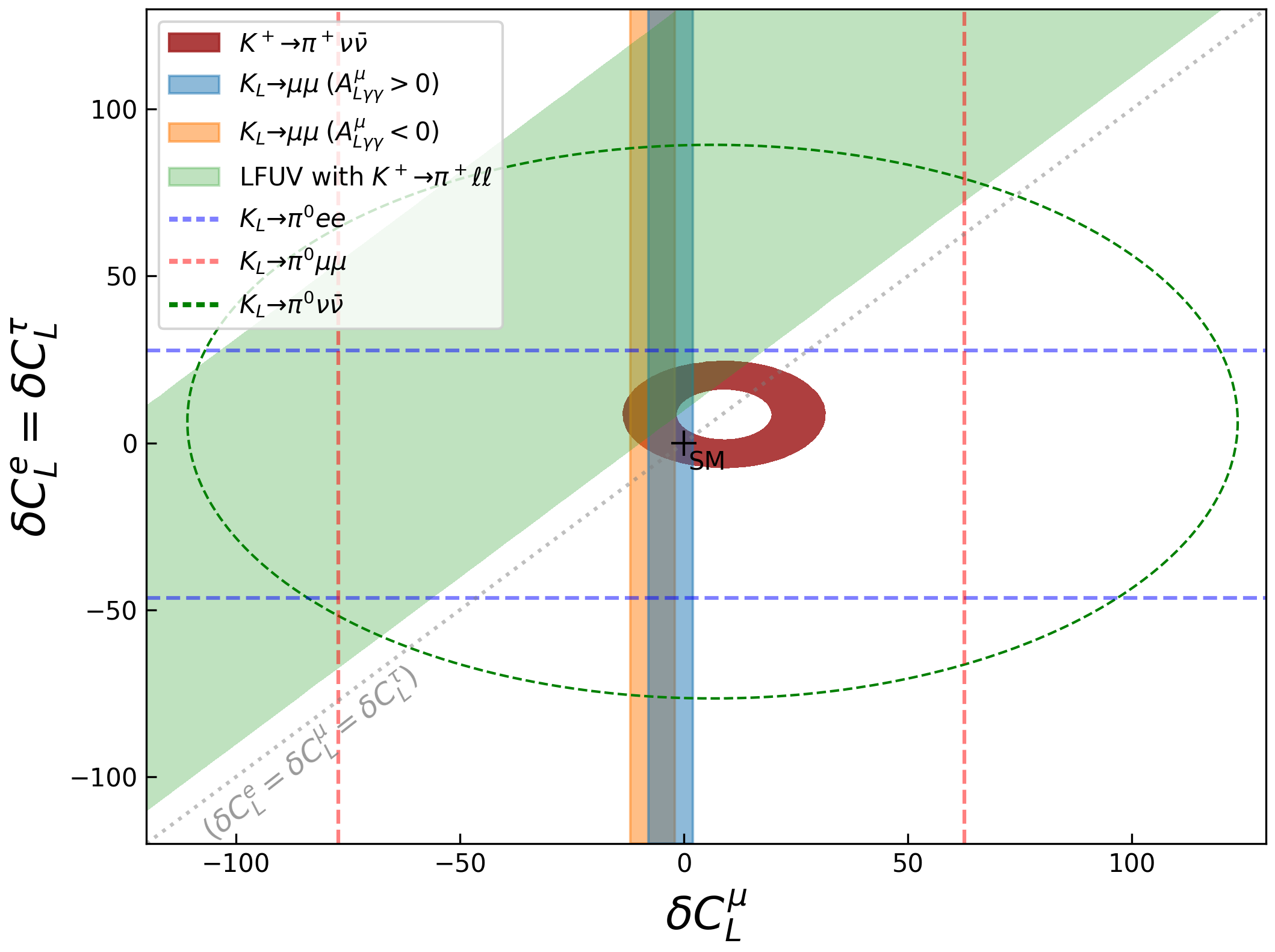
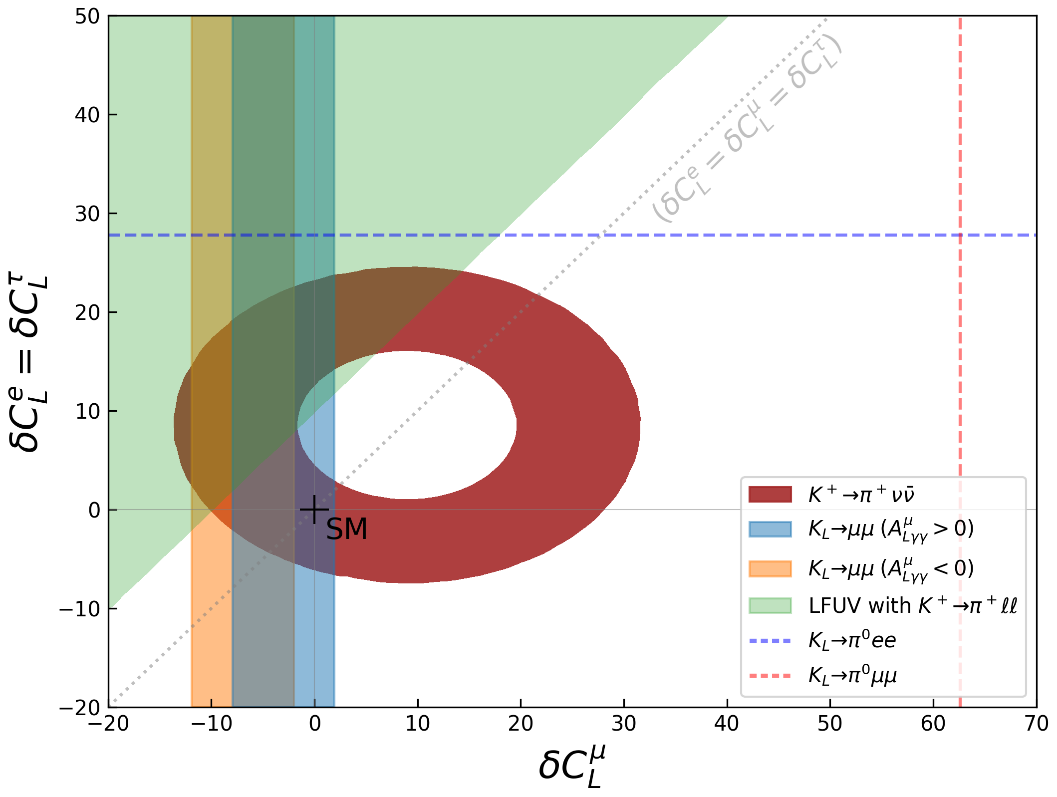
Figure 12: The bounds from individual observables. The right panel is the zoomed version of the left panel. The coloured regions correspond to $68\%$ CL when there is a measurement and the dashed ones to upper limits. $K_{L}\to\mu\bar{\mu}$ has been shown for both signs for the long-distance contribution. For $K_{L}\to\pi^{0}e\bar{e}$ and $K_{L}\to\pi^{0}\mu\bar{\mu}$, constructive interference between direct and indirect CP-violating contributions have been assumed.

In the case of the former, figure 11 illustrates corresponding regions when the New Physics Wilson coefficients for the electron and tau are set equal to each other. This has implications when we present the combination of all observables and is shown in figure 12. In comparison with figure 7, note the flattening of the maroon ellipse which makes the upper bound for $K_{L}\to\pi^{0}e\bar{e}$ less powerful in constraining the regions of the parameter space that were scanned.

Appendix D $Y(x_{t})$ and $Y_{c}$ expressions

The SM expressions of $Y(x_{t})$ is given in ref. Buchalla:1998ba

$$Y(x_{t})=Y_{0}(x_{t})+\frac{\alpha_{s}(\mu_{t})}{4\pi}Y_{1}(x_{t}),$$ (34)

where the LO gauge-independent $Y_{0}(x_{t})\equiv C_{0}(x_{t})-B_{0}(x_{t})$

$$Y_{0}(x)=\frac{x_{t}}{8}\left[\frac{4-x_{t}}{1-x_{t}}+\frac{3x_{t}}{(1-x_{t})^{2}}\log x_{t}\right]$$ (35)

and

$$Y_{1}(x_{t}) =\frac{10x_{t}+10x_{t}^{2}+4x_{t}^{3}}{3(1-x_{t})^{2}}-\frac{2x_{t}-8x_{t}^{2}-x_{t}^{3}-x_{t}^{4}}{(1-x_{t})^{3}}\log x_{t}$$

$$+\frac{2x_{t}-14x_{t}^{2}+x_{t}^{3}-x_{t}^{4}}{2(1-x_{t})^{3}}\log^{2}x_{t}+\frac{2x_{t}+x_{t}^{3}}{(1-x_{t})^{2}}{\rm Li_{2}}(1-x_{t})$$

$$+8x_{t}\frac{\partial Y_{0}}{\partial x_{t}}\log\frac{\mu^{2}}{M^{2}_{W}}.$$ (36)

For the charm contributions, we have $Y_{c}=\lambda^{4}P_{c}(Y)$ where $P_{c}(Y)$ is calculated at NNLO in QCD Gorbahn:2006bm . The analytic expression is not given, however, an approximate formula with $\lambda$-dependence is offered

$$P_{c}(Y) =0.115\pm 0.008_{\rm theor}\pm 0.008_{m_{c}}\pm 0.001_{\alpha_{s}}=\left(0.115\pm 0.018\right)\left(\frac{0.225}{\lambda}\right)^{4}\,,$$ (37)

Another approximate formula with an accuracy of better than $\pm 1.0\%$ in the ranges $1.15\!\text{ GeV}\leq m_{c}(m_{c})\leq 1.45\!\text{ GeV}$, $0.1150\leq\alpha_{s}(M_{Z})\leq 0.1230$, $1.0\!\text{ GeV}\leq\mu_{c}\leq 3.0\!\text{ GeV}$ and $2.5\!\text{ GeV}\leq\mu_{b}\leq 10.0\!\text{ GeV}$ is also given in ref. Gorbahn:2006bm

$$P_{c}(Y) =0.1198\left(\frac{m_{c}(m_{c})}{1.30\!\text{ GeV}}\right)^{2.3595}\left(\frac{\alpha_{s}(M_{Z})}{0.1187}\right)^{6.6055}$$

$$\times\left(1+\sum_{i,j,k,l}\kappa_{ijlm}L_{m_{c}}^{i}L_{\alpha_{s}}^{j}L_{\mu_{c}}^{k}L_{\mu_{b}}^{l}\right)\left(\frac{0.225}{\lambda}\right)^{4},$$ (38)

where

$$L_{m_{c}} =\ln\left(\frac{m_{c}(m_{c})}{1.30\!\text{ GeV}}\right)\,, L_{\alpha_{s}} =\ln\left(\frac{\alpha_{s}(M_{Z})}{0.1187}\right)\,,$$

$$L_{\mu_{c}} =\ln\left(\frac{\mu_{c}}{1.5\!\text{ GeV}}\right)\,, L_{\mu_{b}} =\ln\left(\frac{\mu_{b}}{5.0\!\text{ GeV}}\right)\,,$$ (39)

with

$$\kappa_{1000} =-0.5373, \kappa_{0100}=-6.0472, \kappa_{0010}=-0.0956,$$

$$\kappa_{0001} =0.0114, \kappa_{1100}=3.9957, \kappa_{1010}=0.3604,$$

$$\kappa_{0110} =0.0516, \kappa_{0101}=-0.0658, \kappa_{2000}=-0.1767,$$

$$\kappa_{0200} =16.4465, \kappa_{0020}=-0.1294, \kappa_{0030}=0.0725.$$ (40)

Appendix E The long-distance contribution to $K_{L}\to\mu\bar{\mu}$

The long-distance contributions given in eq. 14 can be written as DAmbrosio:2017klp ; Chobanova:2017rkj

$$N_{L}^{\rm LD} =\frac{\pm 4\,\alpha_{\rm em}\,m_{\mu}}{\pi\,f_{K}\,M_{K}^{2}\,}\sqrt{\frac{2\pi}{M_{K}}\frac{{\rm Br}(K_{L}^{0}\to\gamma\gamma)^{\rm EXP}}{\tau_{L}}}(\chi_{\rm disp}+i\chi_{\rm abs})\,,$$ (41)

with ${\rm Br}(K_{L}^{0}\to\gamma\gamma)^{\rm EXP}=(5.47\pm 0.04)\times 10^{-4}$ PDG2020 , and $(\chi_{\rm disp}+i\chi_{\rm abs})$ corresponding to the $2\gamma$ intermediate state given by DAmbrosio:1986zin ; GomezDumm:1998gw ; Knecht:1999gb ; Isidori:2003ts

$$\chi_{\rm abs} ={\rm Im}\left(C_{\gamma\gamma}\right)=\frac{\pi}{2\beta_{\mu,K}}\ln\left(\frac{1-\beta_{\mu,K}}{1+\beta_{\mu,K}}\right)\,,$$ (42)

$$\chi_{\rm disp} =\chi_{\gamma\gamma}(\mu)-\frac{5}{2}+\frac{3}{2}\ln\left(\frac{m_{\mu}^{2}}{\mu^{2}}\right)+{\rm Re}\left(C_{\gamma\gamma}\right)\,,$$ (43)

with

$$\beta_{\mu,K} =\sqrt{1-4m_{\mu}/M_{K}^{2}}\,,$$ (44)

$$C_{\gamma\gamma} =\frac{1}{\beta_{\mu,K}}\left[{\rm Li}_{2}\left(\frac{\beta_{\mu}-1}{\beta_{\mu}+1}\right)+\frac{\pi^{2}}{3}+\frac{1}{4}\ln^{2}\left(\frac{\beta_{\mu}-1}{\beta_{\mu}+1}\right)\right]\,,$$ (45)

where the low-energy coupling $\chi_{\gamma\gamma}(\mu)$ which depends on the $K_{L}\to\gamma\gamma$ form factor behaviour outside the physical region is estimated in ref. Isidori:2003ts

$$\chi_{\gamma\gamma}(M_{\rho})=5.83\pm 0.15_{\rm exp}\pm 1.0_{\rm th}\,,$$ (46)

resulting in $(\chi_{\rm disp}+i\chi_{\rm abs})=(0.71\pm 0.15\pm 1.0)+i(-5.21)$ Mescia:2006jd .

Appendix F Calculations of theory error

The theoretical errors for $K_{L}\to\mu\bar{\mu}$ and $K_{L}\to\pi^{0}\ell\bar{\ell}$ are characterised by asymmetric uncertainties. In particular, for the former, the degree of departure from the symmetric Gaussian errors was significant for the former and in contrast with the values quoted thus far. In this section, we elaborate on the reasons for this departure and argue why a symmetric Gaussian uncertainty does not accurately reflect the true theoretical uncertainty.

For any given observable, we take into account the latest values of the inputs and the corresponding errors assuming a Gaussian distribution and employing a Monte Carlo simulation for the uncertainty propagation. The blue (orange) distribution in figure 13 gives the probability distribution function (PDF) for the positive (negative) sign of the long-distance contribution for $K_{L}\to\mu\bar{\mu}$. The central values quoted in table 2 reflect the value estimated by using the central values of the inputs given in table 3, while the asymmetric uncertainties are calculated by considering the boundaries between which the area under the PDF curve is $0.68$. This is to be compared with the solid lines which reflect the Gaussian description where $\mu$ and $\sigma$ have been naively calculated from the Monte Carlo distribution without taking into account the asymmetric nature of the distribution. We emphasise the large departure of the symmetric description compared to the Monte Carlo distribution, especially for the case of positive sign for long-distance contributions ($A_{L\gamma\gamma}^{\mu}>0$, shown in blue).

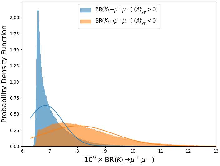
Figure 13: Comparison of the Monte Carlo PDF for $K_{L}\to\mu\bar{\mu}$ with the Gaussian description of the uncertainty.

A similar situation, albeit to a much lesser degree, is also noted for $K_{L}\to\pi^{0}\ell\bar{\ell}$ as shown in figure 14. For completeness, we show the distributions for both the signs of the interference between the direct and indirect CP-violating terms. The difference between the actual distribution and the corresponding naive Gaussian description is only marginal. The values in table 2 reflect the values obtained from the actual asymmetric distribution.

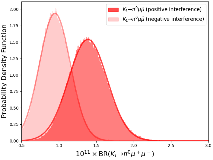
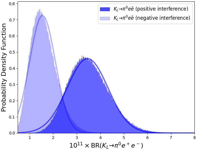
Figure 14: Comparison of the Monte Carlo PDF for $K_{L}\to\pi^{0}\ell\bar{\ell}$ with the Gaussian description of the uncertainty for both positive and negative interference.

References

- (1) Muon g-2 collaboration, Measurement of the Positive Muon Anomalous Magnetic Moment to 0.46 ppm, Phys. Rev. Lett. 126 (2021) 141801 [2104.03281].
- (2) Muon g-2 collaboration, Final Report of the Muon E821 Anomalous Magnetic Moment Measurement at BNL, Phys. Rev. D 73 (2006) 072003 [hep-ex/0602035].
- (3) LHCb collaboration, Test of lepton universality using decays, Phys. Rev. Lett. 113 (2014) 151601 [1406.6482].
- (4) LHCb collaboration, Test of lepton universality with decays, JHEP 08 (2017) 055 [1705.05802].
- (5) Belle collaboration, Test of Lepton-Flavor Universality in Decays at Belle, Phys. Rev. Lett. 126 (2021) 161801 [1904.02440].
- (6) LHCb collaboration, Search for lepton-universality violation in decays, Phys. Rev. Lett. 122 (2019) 191801 [1903.09252].
- (7) LHCb collaboration, Test of lepton universality in beauty-quark decays, Nature Phys. 18 (2022) 277 [2103.11769].
- (8) BaBar collaboration, Measurement of an Excess of Decays and Implications for Charged Higgs Bosons, Phys. Rev. D 88 (2013) 072012 [1303.0571].
- (9) Belle collaboration, Measurement of the branching ratio of relative to decays with hadronic tagging at Belle, Phys. Rev. D 92 (2015) 072014 [1507.03233].
- (10) LHCb collaboration, Measurement of the ratio of branching fractions , Phys. Rev. Lett. 115 (2015) 111803 [1506.08614].
- (11) LHCb collaboration, Measurement of the ratio of the and branching fractions using three-prong -lepton decays, Phys. Rev. Lett. 120 (2018) 171802 [1708.08856].
- (12) Belle collaboration, Measurement of and with a semileptonic tagging method, 1904.08794.
- (13) LHCb collaboration, Observation of the decay , Phys. Rev. Lett. 128 (2022) 191803 [2201.03497].
- (14) J.C. Hardy and I.S. Towner, Superallowed nuclear decays: 2020 critical survey, with implications for Vud and CKM unitarity, Phys. Rev. C 102 (2020) 045501.
- (15) NA62 collaboration, Measurement of the very rare decay, JHEP 06 (2021) 093 [2103.15389].
- (16) L. Bician, New measurement of the decay at NA62, PoS ICHEP2020 (2021) 364.
- (17) KOTO collaboration, Search for the and decays at the J-PARC KOTO experiment, Phys. Rev. Lett. 122 (2019) 021802 [1810.09655].
- (18) T. Hurth, F. Mahmoudi, D.M. Santos and S. Neshatpour, More Indications for Lepton Nonuniversality in , Phys. Lett. B 824 (2022) 136838 [2104.10058].
- (19) M. Algueró, B. Capdevila, S. Descotes-Genon, J. Matias and M. Novoa-Brunet, global fits after and , Eur. Phys. J. C 82 (2022) 326 [2104.08921].
- (20) W. Altmannshofer and P. Stangl, New physics in rare B decays after Moriond 2021, Eur. Phys. J. C 81 (2021) 952 [2103.13370].
- (21) M. Ciuchini, M. Fedele, E. Franco, A. Paul, L. Silvestrini and M. Valli, Lessons from the angular analyses, Phys. Rev. D 103 (2021) 015030 [2011.01212].
- (22) L.-S. Geng, B. Grinstein, S. Jäger, S.-Y. Li, J. Martin Camalich and R.-X. Shi, Implications of new evidence for lepton-universality violation in decays, Phys. Rev. D 104 (2021) 035029 [2103.12738].
- (23) A. Datta, J. Kumar and D. London, The anomalies and new physics in , Phys. Lett. B 797 (2019) 134858 [1903.10086].
- (24) A.K. Alok, A. Dighe, S. Gangal and D. Kumar, Continuing search for new physics in decays: two operators at a time, JHEP 06 (2019) 089 [1903.09617].
- (25) K. Kowalska, D. Kumar and E.M. Sessolo, Implications for new physics in transitions after recent measurements by Belle and LHCb, Eur. Phys. J. C 79 (2019) 840 [1903.10932].
- (26) G. D’Amico, M. Nardecchia, P. Panci, F. Sannino, A. Strumia, R. Torre et al., Flavour anomalies after the measurement, JHEP 09 (2017) 010 [1704.05438].
- (27) A. Crivellin, G. D’Ambrosio, M. Hoferichter and L.C. Tunstall, Violation of lepton flavor and lepton flavor universality in rare kaon decays, Phys. Rev. D 93 (2016) 074038 [1601.00970].
- (28) F. Mahmoudi, SuperIso: A Program for calculating the isospin asymmetry of in the MSSM, Comput. Phys. Commun. 178 (2008) 745 [0710.2067].
- (29) F. Mahmoudi, SuperIso v2.3: A Program for calculating flavor physics observables in Supersymmetry, Comput. Phys. Commun. 180 (2009) 1579 [0808.3144].
- (30) F. Mahmoudi, SuperIso v3.0, flavor physics observables calculations: Extension to NMSSM, Comput. Phys. Commun. 180 (2009) 1718.
- (31) S. Neshatpour and F. Mahmoudi, Flavour Physics with SuperIso, PoS TOOLS2020 (2021) 036 [2105.03428].
- (32) S. Neshatpour and F. Mahmoudi, Flavour Physics Phenomenology with SuperIso, PoS CompTools2021 (2022) 010 [2207.04956].
- (33) E865 collaboration, A New measurement of the properties of the rare decay , Phys. Rev. Lett. 83 (1999) 4482 [hep-ex/9907045].
- (34) NA48/2 collaboration, Precise measurement of the decay, Phys. Lett. B 677 (2009) 246 [0903.3130].
- (35) NA48/2 collaboration, New measurement of the decay, Phys. Lett. B 697 (2011) 107 [1011.4817].
- (36) C. Bobeth and A.J. Buras, Leptoquarks meet and rare Kaon processes, JHEP 02 (2018) 101 [1712.01295].
- (37) D. Rein and L.M. Sehgal, Long Distance Contributions to the Decay , Phys. Rev. D 39 (1989) 3325.
- (38) J.S. Hagelin and L.S. Littenberg, Rare Kaon Decays, Prog. Part. Nucl. Phys. 23 (1989) 1.
- (39) M. Lu and M.B. Wise, Long distance contributions to , Phys. Lett. B 324 (1994) 461 [hep-ph/9401204].
- (40) C.Q. Geng, I.J. Hsu and Y.C. Lin, Comments on long distance contribution to , Phys. Lett. B 355 (1995) 569 [hep-ph/9506313].
- (41) G. Buchalla, A.J. Buras and M.E. Lautenbacher, Weak decays beyond leading logarithms, Rev. Mod. Phys. 68 (1996) 1125 [hep-ph/9512380].
- (42) S. Fajfer, Long distance contribution to decay and terms in CHPT, Nuovo Cim. A 110 (1997) 397 [hep-ph/9602322].
- (43) G. Buchalla and A.J. Buras, and high precision determinations of the CKM matrix, Phys. Rev. D 54 (1996) 6782 [hep-ph/9607447].
- (44) G. Buchalla and A.J. Buras, The rare decays , and : An Update, Nucl. Phys. B548 (1999) 309 [hep-ph/9901288].
- (45) F. Mescia and C. Smith, Improved estimates of rare K decay matrix-elements from Kl3 decays, Phys. Rev. D76 (2007) 034017 [0705.2025].
- (46) M. Misiak and J. Urban, QCD corrections to FCNC decays mediated by Z penguins and W boxes, Phys. Lett. B451 (1999) 161 [hep-ph/9901278].
- (47) J. Brod, M. Gorbahn and E. Stamou, Two-Loop Electroweak Corrections for the Decays, Phys. Rev. D 83 (2011) 034030 [1009.0947].
- (48) J. Brod, M. Gorbahn and E. Stamou, Updated Standard Model Prediction for and , PoS BEAUTY2020 (2021) 056 [2105.02868].
- (49) G. Hiller and F. Kruger, More model-independent analysis of processes, Phys. Rev. D 69 (2004) 074020 [hep-ph/0310219].
- (50) G. D’Ambrosio, G. Ecker, G. Isidori and J. Portoles, The Decays beyond leading order in the chiral expansion, JHEP 08 (1998) 004 [hep-ph/9808289].
- (51) F.J. Gilman and M.B. Wise, in the Six Quark Model, Phys. Rev. D 21 (1980) 3150.
- (52) G. Ecker, A. Pich and E. de Rafael, Radiative Kaon Decays and CP Violation in Chiral Perturbation Theory, Nucl. Phys. B 303 (1988) 665.
- (53) G. Ecker, A. Pich and E. de Rafael, Decays in the Effective Chiral Lagrangian of the Standard Model, Nucl. Phys. B 291 (1987) 692.
- (54) G. D’Ambrosio, G. Ecker, G. Isidori and H. Neufeld, Radiative nonleptonic kaon decays, in DAFNE Physics Handbook, L. Maiani, G. Pancheri and N. Paver, eds., 11, 1994 [hep-ph/9411439].
- (55) B. Ananthanarayan and I. Sentitemsu Imsong, The 27-plet contributions to the CP-conserving decays, J. Phys. G 39 (2012) 095002 [1207.0567].
- (56) J. Kambor, J.H. Missimer and D. Wyler, and decays in next-to-leading order chiral perturbation theory, Phys. Lett. B 261 (1991) 496.
- (57) J. Bijnens, P. Dhonte and F. Borg, decays in chiral perturbation theory, Nucl. Phys. B 648 (2003) 317 [hep-ph/0205341].
- (58) V. Cirigliano, G. Ecker, H. Neufeld, A. Pich and J. Portoles, Kaon Decays in the Standard Model, Rev. Mod. Phys. 84 (2012) 399 [1107.6001].
- (59) E. Coluccio Leskow, G. D’Ambrosio, D. Greynat and A. Nath, form factor in the Large-Nc and cut-off regularization method, Phys. Rev. D 93 (2016) 094031 [1603.09721].
- (60) G. D’Ambrosio, D. Greynat and M. Knecht, On the amplitudes for the CP-conserving rare decay modes, JHEP 02 (2019) 049 [1812.00735].
- (61) G. D’Ambrosio, D. Greynat and M. Knecht, Matching long and short distances at order in the form factors for , Phys. Lett. B 797 (2019) 134891 [1906.03046].
- (62) Z. et al, Review of Particle Physics, Progress of Theoretical and Experimental Physics 2020 (2020) [https://academic.oup.com/ptep/article-pdf/2020/8/083C01/33653179/ptaa104.pdf].
- (63) LHCb collaboration, Constraints on the Branching Fraction, Phys. Rev. Lett. 125 (2020) 231801 [2001.10354].
- (64) G. Isidori and R. Unterdorfer, On the short distance constraints from , JHEP 01 (2004) 009 [hep-ph/0311084].
- (65) V. Chobanova, G. D’Ambrosio, T. Kitahara, M. Lucio Martinez, D. Martinez Santos, I.S. Fernandez et al., Probing SUSY effects in , JHEP 05 (2018) 024 [1711.11030].
- (66) G. Ecker and A. Pich, The Longitudinal muon polarization in , Nucl. Phys. B366 (1991) 189.
- (67) G. D’Ambrosio and T. Kitahara, Direct Violation in , Phys. Rev. Lett. 119 (2017) 201802 [1707.06999].
- (68) F. Mescia, C. Smith and S. Trine, and : A Binary star on the stage of flavor physics, JHEP 08 (2006) 088 [hep-ph/0606081].
- (69) C. Quigg and J.D. Jackson, Decays of Neutral Pseudoscalar Mesons into Lepton Pairs, .
- (70) B.R. Martin, E. De Rafael and J. Smith, Neutral kaon decays into lepton pairs, Phys. Rev. D 2 (1970) 179.
- (71) M.J. Savage, M.E. Luke and M.B. Wise, The Rare decays , and in chiral perturbation theory, Phys. Lett. B 291 (1992) 481 [hep-ph/9207233].
- (72) G. D’Ambrosio, M. Miragliuolo and P. Santorelli, Radiative nonleptonic kaon decays, .
- (73) G. D’Ambrosio and G. Isidori, CP violation in kaon decays, Int. J. Mod. Phys. A 13 (1998) 1 [hep-ph/9611284].
- (74) G. Valencia, Long distance contribution to , Nucl. Phys. B 517 (1998) 339 [hep-ph/9711377].
- (75) G. D’Ambrosio, G. Isidori and J. Portoles, Can we extract short distance information from B?, Phys. Lett. B 423 (1998) 385 [hep-ph/9708326].
- (76) M. Gorbahn and U. Haisch, Charm Quark Contribution to at Next-to-Next-to-Leading, Phys. Rev. Lett. 97 (2006) 122002 [hep-ph/0605203].
- (77) LHCb collaboration, Physics case for an LHCb Upgrade II - Opportunities in flavour physics, and beyond, in the HL-LHC era, 1808.08865.
- (78) A. Dery, M. Ghosh, Y. Grossman and S. Schacht, as a clean probe of short-distance physics, JHEP 07 (2021) 103 [2104.06427].
- (79) G. Buchalla, G. D’Ambrosio and G. Isidori, Extracting short distance physics from decays, Nucl. Phys. B 672 (2003) 387 [hep-ph/0308008].
- (80) G. Isidori, C. Smith and R. Unterdorfer, The Rare decay within the SM, Eur. Phys. J. C 36 (2004) 57 [hep-ph/0404127].
- (81) J.F. Donoghue, B.R. Holstein and G. Valencia, as a Probe of CP Violation, Phys. Rev. D 35 (1987) 2769.
- (82) G. Ecker, A. Pich and E. de Rafael, Decays in Chiral Perturbation Theory, Phys. Lett. B 189 (1987) 363.
- (83) L.M. Sehgal, CP Violation in : Interference of One Photon and Two Photon Exchange, Phys. Rev. D 38 (1988) 808.
- (84) J. Flynn and L. Randall, The CP Conserving Long Distance Contribution to the Decay , Phys. Lett. B 216 (1989) 221.
- (85) L. Cappiello and G. D’Ambrosio, Decay in the Chiral Effective Lagrangian, Nuovo Cim. A 99 (1988) 155.
- (86) T. Morozumi and H. Iwasaki, The CP Conserving Contribution in the Decays and , Prog. Theor. Phys. 82 (1989) 371.
- (87) G. Ecker, A. Pich and E. de Rafael, Vector Meson Exchange in Radiative Kaon Decays and Chiral Perturbation Theory, Phys. Lett. B 237 (1990) 481.
- (88) L. Cappiello, G. D’Ambrosio and M. Miragliuolo, Corrections to from , Phys. Lett. B 298 (1993) 423.
- (89) P. Heiliger and L.M. Sehgal, Analysis of the decay and expectations for the decays and , Phys. Rev. D 47 (1993) 4920.
- (90) A.G. Cohen, G. Ecker and A. Pich, Unitarity and , Phys. Lett. B 304 (1993) 347.
- (91) A.J. Buras, M.E. Lautenbacher, M. Misiak and M. Munz, Direct CP violation in beyond leading logarithms, Nucl. Phys. B 423 (1994) 349 [hep-ph/9402347].
- (92) G. D’Ambrosio and J. Portoles, Vector meson exchange contributions to and , Nucl. Phys. B 492 (1997) 417 [hep-ph/9610244].
- (93) J.F. Donoghue and F. Gabbiani, and its relation to CP and chiral tests, Phys. Rev. D 56 (1997) 1605 [hep-ph/9702278].
- (94) KTeV collaboration, Measurement of the decay , Phys. Rev. Lett. 83 (1999) 917 [hep-ex/9902029].
- (95) K. Murakami et al., Experimental search for the decay mode , Phys. Lett. B 463 (1999) 333 [hep-ex/9907007].
- (96) KTeV collaboration, First observation of the decay , Phys. Rev. Lett. 87 (2001) 021801 [hep-ex/0011093].
- (97) M.V. Diwan, H. Ma and T.L. Trueman, Muon decay asymmetries from decays, Phys. Rev. D 65 (2002) 054020 [hep-ph/0112350].
- (98) F. Gabbiani and G. Valencia, and the bound on the CP conserving , Phys. Rev. D 64 (2001) 094008 [hep-ph/0105006].
- (99) F. Gabbiani and G. Valencia, Vector meson contributions do not explain the rate and spectrum in , Phys. Rev. D 66 (2002) 074006 [hep-ph/0207189].
- (100) NA48 collaboration, Precise measurement of the decay , Phys. Lett. B 536 (2002) 229 [hep-ex/0205010].
- (101) R.S. Chivukula, H. Georgi and L. Randall, A Composite Technicolor Standard Model of Quarks, Nucl. Phys. B 292 (1987) 93.
- (102) L.J. Hall and L. Randall, Weak scale effective supersymmetry, Phys. Rev. Lett. 65 (1990) 2939.
- (103) R. Rattazzi and A. Zaffaroni, Comments on the holographic picture of the Randall-Sundrum model, JHEP 04 (2001) 021 [hep-th/0012248].
- (104) A.J. Buras, P. Gambino, M. Gorbahn, S. Jager and L. Silvestrini, Universal unitarity triangle and physics beyond the standard model, Phys. Lett. B 500 (2001) 161 [hep-ph/0007085].
- (105) G. D’Ambrosio, G.F. Giudice, G. Isidori and A. Strumia, Minimal flavor violation: An Effective field theory approach, Nucl. Phys. B 645 (2002) 155 [hep-ph/0207036].
- (106) C. Bobeth, A.J. Buras, A. Celis and M. Jung, Patterns of Flavour Violation in Models with Vector-Like Quarks, JHEP 04 (2017) 079 [1609.04783].
- (107) KTeV collaboration, Search for the rare decay , Phys. Rev. Lett. 93 (2004) 021805 [hep-ex/0309072].
- (108) KTEV collaboration, Search for the Decay , Phys. Rev. Lett. 84 (2000) 5279 [hep-ex/0001006].
- (109) E. Goudzovski et al., New Physics Searches at Kaon and Hyperon Factories, 2201.07805.
- (110) G. Buchalla et al., , and decays, Eur. Phys. J. C 57 (2008) 309 [0801.1833].
- (111) A.A. Alves Junior et al., Prospects for Measurements with Strange Hadrons at LHCb, JHEP 05 (2019) 048 [1808.03477].
- (112) NA62, KLEVER collaboration, Rare decays at the CERN high-intensity kaon beam facility, 2009.10941.
- (113) E. Goudzovski and E. Passemar, Seminar at RPF spring meeting,Cincinnati, 16-19 May 2022, .
- (114) Flavour Lattice Averaging Group collaboration, FLAG Review 2019: Flavour Lattice Averaging Group (FLAG), Eur. Phys. J. C 80 (2020) 113 [1902.08191].
- (115) G. Buchalla and A.J. Buras, QCD corrections to rare K and B decays for arbitrary top quark mass, Nucl. Phys. B400 (1993) 225.
- (116) A.J. Buras, D. Buttazzo, J. Girrbach-Noe and R. Knegjens, and in the Standard Model: status and perspectives, JHEP 11 (2015) 033 [1503.02693].
- (117) T. Inami and C.S. Lim, Effects of Superheavy Quarks and Leptons in Low-Energy Weak Processes and , Prog. Theor. Phys. 65 (1981) 297.
- (118) G. Buchalla, A.J. Buras and M.K. Harlander, Penguin box expansion: Flavor changing neutral current processes and a heavy top quark, Nucl. Phys. B349 (1991) 1.
- (119) J. Brod and M. Gorbahn, Electroweak Corrections to the Charm Quark Contribution to , Phys. Rev. D78 (2008) 034006 [0805.4119].
- (120) G. D’Ambrosio and D. Espriu, Rare Decay Modes of the K Mesons in the Chiral Lagrangian, Phys. Lett. B 175 (1986) 237.
- (121) D. Gomez Dumm and A. Pich, Long distance contributions to the decay width, Phys. Rev. Lett. 80 (1998) 4633 [hep-ph/9801298].
- (122) M. Knecht, S. Peris, M. Perrottet and E. de Rafael, Decay of pseudoscalars into lepton pairs and large QCD, Phys. Rev. Lett. 83 (1999) 5230 [hep-ph/9908283].