Quantum Liouvillian exceptional and diabolical points for bosonic fields with quadratic Hamiltonians: The Heisenberg-Langevin equation approach

Abstract

Equivalent approaches to determine eigenfrequencies of the Liouvillians of open quantum systems are discussed using the solution of the Heisenberg-Langevin equations and the corresponding equations for operator moments. A simple damped two-level atom is analyzed to demonstrate the equivalence of both approaches. The suggested method is used to reveal the structure as well as eigenfrequencies of the dynamics matrices of the corresponding equations of motion and their degeneracies for interacting bosonic modes described by general quadratic Hamiltonians. Quantum Liouvillian exceptional and diabolical points and their degeneracies are explicitly discussed for the case of two modes. Quantum hybrid diabolical exceptional points (inherited, genuine, and induced) and hidden exceptional points, which are not recognized directly in amplitude spectra, are observed. The presented approach via the Heisenberg-Langevin equations paves the general way to a detailed analysis of quantum exceptional and diabolical points in infinitely dimensional open quantum systems.

1 Introduction

Non-Hermitian Hamiltonians, for systems with properly balanced dissipation and amplification, have real energy spectra if they exhibit the parity-time ($\cal PT$) symmetry, as shown by Bender and Boettcher [1]. That discovery has lead to the development of non-Hermitian quantum mechanics [2, 3, 4, 5] and has triggered impressive research interest ranging from studying fundamental aspects of quantum physics [6, 7, 8, 9, 10, 11] to proposing applications in quantum metrology, optics, optomechanics, and photonics [12, 13, 14]. Studies of non-Hermitian quantum mechanics include also finding quantum analogues of general relativity concepts (like Einstein’s quantum elevator [15]), proving various no-go theorems for information processing with non-Hermitian systems [16, 17], and even proposals to apply specific non-Hermitian systems, with energy spectra corresponding to the zeros of the Riemann zeta function, aimed at proving the Riemann hypothesis [18].

Recently, a considerable interest in studying non-Hermitian systems has been focused on their exceptional points (EPs), which occur, e.g., at the phase transitions between the $\cal PT$ and non-$\cal PT$ regimes. Various applications of EPs for refined quantum control of dissipative and/or amplified systems have been proposed (for reviews see [19, 20, 14] and references therein).

Most of these studies on EPs are limited to Hamiltonian EPs, which correspond to the degeneracies of the eigenvalues of non-Hermitian Hamiltonians associated with their coalescent eigenvectors. We note that these EPs may be called semiclassical, because they are not affected by quantum jumps, as explicitly discussed in [21] based on the quantum-trajectory theory [22], which is also referred to as the Monte Carlo wave-function method [23, 24] or the quantum-jump approach [25]. Indeed, non-Hermitian Hamiltonians describe only a continuous nonunitary dissipation of an open system, but its full quantum description requires also the inclusion of quantum jumps in the system evolution. Recently, these semiclassical Hamiltonian EPs have been generalized to the quantum regime by analyzing the EPs of quantum Liouvillians instead of those of non-Hermitian Hamiltonians [21]. Specifically, quantum EPs (QEPs) can be defined as the degeneracies of the eigenvalues corresponding to coalescent eigenmatrices (eigenoperators) of the quantum Liouvillian superoperator for a Lindblad master equation. Clearly, such an approach to EPs includes the effect of quantum jumps, as it is based on the standard master-equation approach [26] with a trivial metric for arbitrary systems. In contrast to this, a complete description of the evolution of a non-Hermitian system within the Bender-Boettcher quantum mechanics requires also calculating the evolution of a nontrivial metric of the system. This is rather complicated and nonintuitive, but necessary to obtain physical results without violating any no-go theorems [16, 17]. The effects of quantum jumps on QEPs have been recently confirmed experimentally in [27, 28].

QEPs and Hamiltonian EPs are, in general, different, although they can be equivalent for classical-like systems (e.g., linearly coupled harmonic oscillators [21]) or specific finite-dimensional systems [29]. Anyway, one can experimentally observe the transition of QEPs into Hamiltonian EPs by a proper postselection of quantum trajectories within the hybrid-Liouvillian formalism of Ref. [30]. We also note that if the eigenvectors corresponding to degenerate eigenvalues of Hamiltonians or Liouvillians do not coalesce, then such points are refereed to as diabolical points. These points have also wide applications in witnessing quantum effects including phase transitions. For example, quantum Liouvillian diabolical points can reveal dissipative phase transitions and a Liouvillian spectral collapse [31, 32].

For the above reasons, the determination of QEPs and their properties represents an important task, which can lead to applications in quantum technologies, including quantum metrology. Unfortunately, the standard approach of finding QEPs via the eigenvalue problem of Liouvillians becomes quite inefficient for multi-qubit or multi-level quantum systems. For systems with infinitely-dimensional Hilbert spaces, the determination of EPs and QEPs is even more challenging. Here, we develop an efficient method based on the Heisenberg-Langevin equations for finding QEPs, and we show the equivalence of QEPs found by these two approaches. We apply the developed method for the determination of QEPs for a system of $M$ bosonic modes mutually interacting via quadratic nonlinear Hamiltonians. Such Hamiltonians are appealing as they lead to the linear exactly-soluble Heisenberg operator equations and, simultaneously, allow to describe nonclassical optical fields including squeezed [33] and sub-Poissonian fields [34]. Such fields are analyzed in the framework of a generalized superposition of a signal and noise [35] that describes quantum Gaussian fields.

The applied method uses the analysis of the dynamical equations for the moments of field operators. It is based upon the equivalence of the eigenfrequency analysis of the Liouvillian and the analysis of an arbitrary complete set of operators of measurable quantities. In the case of quadratic Hamiltonians the field operators moments (FOMs) can be chosen as a suitable set of such measurable operators. These moments form specific structures [36, 37, 38] that exhibit QEPs of varying (exceptional) degeneracies [QEP degeneracies] and multiplicities [diabolical degeneracies (QDP degeneracies) for quantum hybrid diabolical exceptional points (QHPs)]. Contrary to other more general Hamiltonians, the first-order FOMs of quadratic Hamiltonians form a closed set of dynamical equations. Moreover, the eigenfrequencies obtained from these equations allow for the determination of those for higher-order FOMs. These FOMs then provide a complete structure of eigenfrequencies whose numbers increase with the increasing order of the moments. Among others, this results in the identification of eigenfrequencies with infinite QEP and QDP degeneracies forming QEPs and QHPs. There also occur cases in which degenerate eigenfrequencies remain the same at a QEP, i.e. this QEP is not identified by the spectrum. We may refer to hidden quantum exceptional points (hidden QEPs).

The paper is organized as follows. The equivalence of the system eigenfrequencies analyses based on the Liouvillian and Heisenberg equations for the operators of measurable quantities is discussed in general in Sec. II. Both approaches are compared in Sec. III by considering a simple system of a damped two-level atom. Section IV is devoted to the application of the Heisenberg-Langevin equations for an $M$-mode bosonic system with a quadratic Hamiltonian and the eigenfrequency analysis of the equations for FOMs. The eigenfrequencies and their general structure are discussed in Sec. V by considering a two-mode bosonic system with a general quadratic Hamiltonian. Conclusions are drawn in Sec. VI. The correspondence between the generalized master equation and the Heisenberg-Langevin equations is discussed in Appendix A.

2 Equivalence of eigenfrequency analyses in the spaces of statistical operators and measurable operators

Before we address the analysis of QEPs for specific models, we show that the eigenfrequency analysis of a Liouvillian $\hat{\cal L}$ in the space of statistical operators can be equivalently replaced by the eigenfrequency analysis for an arbitrary complete set of measurable operators. The equivalence of projection operator techniques, used for the derivation of generalized master equations with their Liouvillians, and the set of the Heisenberg equations is discussed in detail in [39, 40, 41]. The Liouvillian superoperator $\hat{\cal L}\cdot\equiv-i/\hbar[\hat{H},\cdot]$, where $\cdot$ stands for an arbitrary operator, $[,]$ denotes the commutator, and $\hbar$ means the reduced Planck constant, is defined in terms of the overall Hamiltonian $\hat{H}$ involving the system and its reservoir in its complete description. It is used to evolve the statistical operator $\hat{\rho}(t)$ according to the Liouville equation

$$\frac{d\hat{\rho}(t)}{dt}=\hat{\cal L}\hat{\rho}(t).$$ (1)

We consider an $N$-dimensional Hilbert space with an arbitrary basis $|j\rangle$ for $j=1,\ldots,N$. The corresponding basis in the Liouville space of a statistical operator $\hat{\rho}$ is formed by vectors $\hat{\rho}_{jk}\equiv|j\rangle\langle k|$. They allow to express $\hat{\rho}$ in terms of coefficients $\rho_{jk}$ as follows:

$$\hat{\rho}(t)=\sum_{jk}\rho_{jk}(t)\hat{\rho}_{jk}.$$ (2)

The Liouville equation in (1) transforms into the following set of equations for the coefficients $\rho_{jk}$:

$$\frac{d\rho_{mn}(t)}{dt}=\sum_{jk}{\cal L}_{jk}^{mn}\rho_{jk}(t),$$ (3)

and ${\cal L}_{jk}^{mn}=\langle m|(\hat{\cal L}|j\rangle\langle k|)|n\rangle$. The diagonalization of the matrix ${\cal L}_{jk}^{mn}$ provides us complex eigenvalues $-i\Omega^{\alpha}$ that define eigenfrequencies $\Omega^{\alpha}$. The corresponding eigenvectors $l_{jk}^{\alpha}$ form the eigenoperators $\hat{l}^{\alpha}=\sum_{jk}l_{jk}^{\alpha}|j\rangle\langle k|$. It holds for an anti-Hermitian superoperator $\hat{\cal L}$ that for any eigenvalue $-i\Omega_{\alpha}$ with eigenoperator $\hat{l}^{\alpha}$ there also exists the eigenvalue $i\Omega_{\alpha}^{*}$ with the corresponding eigenoperator $\hat{l}^{\dagger\alpha}$. Moreover the Liouvillians $\hat{\cal L}$ have one eigenfrequency $\Omega_{0}=0$ with the Hermitian eigenoperator $\hat{l}^{0}=\hat{l}^{\dagger 0}$ and ${\rm Tr}\{\hat{l}^{0}\}=1$ that describes the steady state. Contrary to $\hat{l}^{0}$, the remaining eigenoperators $\hat{l}^{\alpha}$ are non-Hermitian and obey ${\rm Tr}\{\hat{l}^{\alpha}\}=0$.

In parallel to Eq. (2), an arbitrary statistical operator $\hat{\rho}$ can be decomposed in the basis $\hat{l}^{\alpha}$ as follows

$$\hat{\rho}(t)=\sum_{\alpha}\big{[}\rho^{\alpha}(t)\hat{l}^{\alpha}+\rho^{\alpha*}(t)\hat{l}^{\alpha\dagger}\big{]},$$ (4)

where $\rho^{\alpha}(t)={\rm Tr}\{\hat{\rho}(t)\hat{l}^{\alpha\dagger}\}$. The evolution of the statistical operator $\hat{\rho}(t)$ is then expressed along the formula

$$\hat{\rho}(t)=\sum_{\alpha}\big{[}\exp(-i\Omega_{\alpha}t)\rho^{\alpha}(0)\hat{l}^{\alpha}+\exp(i\Omega_{\alpha}^{*}t)\rho^{\alpha*}(0)\hat{l}^{\alpha\dagger}\big{]}$$ (5)

that ‘separates’ the evolution for different eigenfrequencies $\Omega_{\alpha}$ and $-\Omega_{\alpha}^{*}$. The coefficients $\rho^{\alpha}(0)$ in Eq. (5) characterize the initial state. The mean value $\langle A\rangle(t)$ of an arbitrary Hermitian operator $\hat{A}(0)$ of a measurable quantity is then determined in the Schrödinger picture as

$$\langle A\rangle(t)\equiv{\rm Tr}\{\hat{\rho}(t)\hat{A}(0)\}=\sum_{\alpha}\big{[}\exp(-i\Omega_{\alpha}t)\rho^{\alpha}(0)A^{\alpha*}(0)+\exp(i\Omega_{\alpha}^{*}t)\rho^{\alpha*}(0)A^{\alpha}(0)\big{]},$$ (6)

using Eq. (5) and the coefficients $A^{\alpha}(0)={\rm Tr}\{\hat{A}(0)\hat{l}^{\alpha\dagger}\}$.

Now let us consider an arbitrary Hermitian operator $\hat{A}(t)$ of a measurable quantity and its evolution in the Heisenberg picture according to the Heisenberg equation

$$\frac{d\hat{A}(t)}{dt}=-\hat{\cal L}\hat{A}(t).$$ (7)

The eigenoperators of the superoperator $-{\cal L}$ coincide with those of ${\cal L}$ and the corresponding eigenvalues differ by sign. Decomposing the operator $\hat{A}(0)$ at $t=0$ into the basis $\hat{l}^{\alpha}$,

$$\hat{A}(0)=\sum_{\alpha}\big{[}A^{\alpha}(0)\hat{l}^{\alpha}+A^{\alpha*}(0)\hat{l}^{\alpha\dagger}\big{]},$$ (8)

we may express the solution of the Heisenberg equation (7) as follows:

$$\hat{A}(t)=\sum_{\alpha}\big{[}\exp(i\Omega_{\alpha}t)A^{\alpha}(0)\hat{l}^{\alpha}+\exp(-i\Omega_{\alpha}^{*}t)A^{\alpha*}(0)\hat{l}^{\dagger\alpha}\big{]}.$$ (9)

Using Eq. (9), the mean value $\langle A\rangle(t)$ of the operator $\hat{A}$ in the Heisenberg picture is expressed in terms of the coefficient $\rho^{\alpha}(0)$ of the initial statistical operator $\hat{\rho}(0)$:

$$\langle A\rangle(t)\equiv{\rm Tr}\{\hat{\rho}(0)\hat{A}(t)\}=\sum_{\alpha}\big{[}\exp(i\Omega_{\alpha}t)\rho^{\alpha*}(0)A^{\alpha}(0)+\exp(-i\Omega_{\alpha}^{*}t)\rho^{\alpha}(0)A^{\alpha*}(0)\big{]}.$$ (10)

Provided that the Liouvillian $\hat{\cal L}$ is constructed using a Hermitian Hamiltonian $\hat{H}$ the eigenfrequencies $\Omega^{\alpha}$ are real and the formulas for the mean values $\langle A\rangle(t)$ in Eqs. (6) and (10) coincide. This means that the time evolution of the operator $\hat{A}(t)$ is described only by the eigenfrequencies $\Omega_{\alpha}$ and $-\Omega_{\alpha}$ known from the evolution of the statistical operator $\hat{\rho}$ fulfilling Eq. (1). Once we construct an arbitrary basis from the Hermitian operators $\hat{A}$ of measurable quantities and analyze the evolution of their mean values $\langle A\rangle(t)$, we reveal all the eigenfrequencies $\Omega_{\alpha}$. The used basis can even be chosen more generally involving also non-Hermitian operators $\hat{A}$.

When deriving a master equation for the reduced statistical operator $\hat{\rho}^{\rm s}$, by tracing out the part of the whole statistical operator $\hat{\rho}$ belonging to the reservoir, we apply the perturbation solution of the general Liouville equation (1) valid up to the second power of the interaction Hamiltonian between the system and its reservoir. This results in a new Liouvillian $\hat{\cal L}^{\rm s}$ that has a more general form compared to that expressed as a commutator with the Hamiltonian $\hat{H}$. We may diagonalize this more general form of the system Liouvillian $\hat{\cal L}^{\rm s}$ to reveal, in general, complex eigenvalues $-\Omega_{\alpha}$ and $\Omega_{\alpha}^{*}$ and the accompanying eigenoperators $\hat{l}^{\alpha}$ and $\hat{l}^{\alpha\dagger}$. Alternatively, we convert the system Liouville equation in Eq. (1) into a coupled set of differential equations for the mean values $\langle A\rangle(t)$ of operators $\hat{A}$ that form a basis in the space of system operators of measurable quantities. According to Eq. (6), the complex eigenfrequencies of the dynamics matrix of this set of differential equations coincide with the eigenfrequencies revealed by a direct diagonalization of the system Liouvillian $\hat{\cal L}^{\rm s}$. For details, see Appendix A. The differential equations for the mean values $\langle A\rangle(t)$ can alternatively be derived from a closed set of the Heisenberg equations written for both the system operators $\hat{A}$ forming the basis and operators of the reservoir. The reservoir operators can suitably be eliminated keeping the validity of the solution up to the second power of the interaction Hamiltonian. This leads to the Heisenberg-Langevin equations. This method known as the Wigner-Weisskopf model of damping [35] for a bosonic mode interacting with bosonic reservoir provides equivalent derivation of the differential equations for the mean values $\langle A\rangle(t)$. This stems from the above discussed equivalence of both descriptions in the Schrödinger and Heisenberg pictures, and equivalent approximations when eliminating the reservoir degrees of freedom [42].

The use of the Heisenberg equations for suitable operators instead of the master equation may provide qualitative advantage compared to the eigenfrequency analysis of the Liouvillian. We demonstrate this by analysing two important examples: a damped two-level atom in Sec. III and the system of mutually interacting bosonic modes with the quadratic interaction Hamiltonian in Secs. IV and V. Whereas the analysis of a damped two-level atom in a finite-dimensional Liouville space leads to a deeper insight into the method based on the Heisenberg equations by its comparison with a direct diagonalization of the Liouvillian, we reveal the structure and values of eigenfrequencies in the model of bosonic modes relying just on the Heisenberg equations.

3 Eigenfrequency analyses of a damped two-level atom

We demonstrate the above discussed equivalence of both approaches in the determination of the system eigenfrequencies by analyzing, probably, the simplest possible physical system — a damped two-level atom. Its Liouville space of statistical operators has dimension 4 and so its Liouvillian ${\cal L}$ has 4 eigenfrequencies and eigenoperators. Moreover, as the system is finite dimensional, powers of the operators of measurable quantities do not play an important role in the eigenfrequency analysis because they are just a linear superposition of operators from any chosen basis in the space of measurable operators. The eigenfrequency analysis performed by both approaches also results in their detailed comparison.

The considered two-level atom has the ground state $|0\rangle$ and the excited state $|1\rangle$. It is described by the Pauli operators $\hat{\sigma}_{x}=\hat{\sigma}_{+}+\hat{\sigma}_{-}$, $\hat{\sigma}_{y}=(\hat{\sigma}_{+}-\hat{\sigma}_{-})/i$ and $\hat{\sigma}_{z}=\hat{\sigma}_{1}-\hat{\sigma}_{0}$; $\hat{\sigma}_{0}\equiv|0\rangle\langle 0|$, $\hat{\sigma}_{1}\equiv|1\rangle\langle 1|$, $\hat{\sigma}_{+}\equiv|1\rangle\langle 0|$, and $\hat{\sigma}_{-}\equiv|0\rangle\langle 1|$. Hamiltonian $\hat{H}^{\rm s}$ of the two-level atom with the excitation energy $\hbar\omega$ is written as

$$\hat{H}^{\rm s}=\hbar\omega\hat{\sigma}_{z}/2.$$ (11)

3.1 Analysis via the Liouvillian superoperator

We begin with the eigenfrequency analysis of the corresponding Liouvillian. We assume that the atom is damped via the interaction with a reservoir based on the $\hat{\sigma}_{x}$ operator. The corresponding Liouvillian $\hat{\cal L}_{x}$ is derived in the form

$$\hat{\cal L}_{x}\cdot=\gamma_{x}\left[\hat{\sigma}_{x}\cdot\hat{\sigma}_{x}-1\cdot\right],$$ (12)

where the dot $\cdot$ stands for an arbitrary operator. For a more general form of damping and the corresponding analysis of the Liouvillian, see [21].

Expressing the statistical operator $\hat{\rho}^{\rm s}$ of the two-level atom in a suitable basis,

$$\hat{\rho}^{\rm s}=\rho_{00}^{\rm s}|0\rangle\langle 0|+\rho_{01}^{\rm s}|0\rangle\langle 1|+\rho_{10}^{\rm s}|1\rangle\langle 0|+\rho_{11}^{\rm s}|1\rangle\langle 1|,$$ (13)

we transform the Liouville equation (1) into the following set of linear differential equations for the coefficients of the decomposition:

$$\frac{d}{dt}\left[\begin{array}[]{c}\rho_{00}^{\rm s}\\ \rho_{01}^{\rm s}\\ \rho_{10}^{\rm s}\\ \rho_{11}^{\rm s}\end{array}\right]=-i{\bf M}\left[\begin{array}[]{c}\rho_{00}^{\rm s}\\ \rho_{01}^{\rm s}\\ \rho_{10}^{\rm s}\\ \rho_{11}^{\rm s}\end{array}\right],$$ (22)

$${\bf M}=\left[\begin{array}[]{cccc}-i\gamma_{x}&0&0&i\gamma_{x}\\ 0&-\omega-i\gamma_{x}&i\gamma_{x}&0\\ 0&i\gamma_{x}&\omega-i\gamma_{x}&0\\ i\gamma_{x}&0&0&-i\gamma_{x}\end{array}\right].$$ (27)

The dynamics matrix ${\bf M}$ defined in Eq. (27) has 4 eigenfrequencies:

$$\Omega_{0}^{\rm s}=0,\hskip 14.22636pt\Omega_{1,2}^{\rm s}=\pm\Omega^{\rm s}-i\gamma_{x},\hskip 14.22636pt\Omega_{3}^{\rm s}=-2i\gamma_{x},$$ (28)

where $\Omega^{\rm s}=\sqrt{\omega^{2}-\gamma_{x}^{2}}$. The eigenfrequencies $\Omega_{1,2}^{\rm s}$ identify a possible QEP for

$$\omega=\gamma_{x}.$$ (29)

We may also determine the corresponding eigenvectors that are conveniently written as columns of the transformation matrix ${\bf P}$:

$${\bf P}=\frac{1}{2}\left[\begin{array}[]{cccc}1&0&0&1\\ 0&i\gamma_{x}&i\gamma_{x}&0\\ 0&\omega+\Omega^{\rm s}&\omega-\Omega^{\rm s}&0\\ 1&0&0&-1\end{array}\right].$$ (30)

We note that the first eigenvector $\hat{\rho}_{0}^{\rm s}$ for $\Omega_{0}^{\rm s}$ that describes the stationary state is normalized such that ${\rm Tr}\{\hat{\rho}_{0}^{\rm s}\}=1$. All other eigenvectors are traceless (${\rm Tr}\{\hat{\rho}_{j}^{\rm s}\}=0$ for $j=1,2,3$) and no specific norm is introduced to normalize them. We have $\Omega^{\rm s}=0$ for the condition in Eq. (29) and so the second and third eigenvectors (columns) in the matrix ${\bf P}$ in Eq. (30) coalesce confirming the presence of an QEP.

3.2 Analysis via the Heisenberg-Langevin equations

Now let us apply the second approach. To derive the appropriate Heisenberg-Langevin equations we need to specify the system interaction with the reservoir represented by a large group of two-level atoms. Their Hamiltonian $\hat{H}^{\rm r}_{0}$ and a suitable interaction Hamiltonian $\hat{H}^{\rm r}_{\rm int}$ are expressed as:

$$\hat{H}^{\rm r}_{0}=\hbar\sum_{j}\omega_{j}^{\rm r}\hat{\sigma}_{j,z}^{\rm r}/2,\hskip 14.22636pt\hat{H}^{\rm r}_{\rm int}=\hbar\sum_{j}\kappa_{j}^{\rm r}\hat{\sigma}_{j,x}^{\rm r}\hat{\sigma}_{x},$$ (31)

where $\omega_{j}^{\rm r}$ stands for the frequency of the $j$th reservoir two-level atom that is coupled with the analyzed two-level atom via the real coupling constant $\kappa_{j}^{\rm r}$. The Pauli operators of the reservoir two-level atoms are introduced in analogy to those of the analyzed system.

We may write the Heisenberg equations for both analyzed two-level atom and reservoir two-level atoms described by the overall Hamiltonian $\hat{H}^{\rm s}+\hat{H}^{\rm r}_{\rm int}+\hat{H}^{\rm r}_{0}$. A systematic elimination of the reservoir operators then results in the following Heisenberg-Langevin equation for an arbitrary operator $\hat{X}$ [42]:

$$\frac{d\hat{X}(t)}{dt}=\frac{i}{\hbar}[\hat{H}^{\rm s}(t),\hat{X}(t)]-\gamma_{x}/2[[\hat{X}(t),\sigma_{x}(t)],\sigma_{x}(t)]-i[\hat{X}(0),\sigma_{x}(0)]\hat{F}_{x}(t).$$ (32)

In Eq. (32) the Langevin operator force $\hat{F}_{x}(t)$, defined as

$$\hat{F}_{x}(t)=\exp(-i\hat{H}^{\rm r}_{0}t/\hbar)\sum_{j}\kappa_{j}^{\rm r}\hat{\sigma}_{j,x}^{\rm r}(0)\exp(i\hat{H}^{\rm r}_{0}t/\hbar),$$ (33)

represents the back-action of the reservoir two-level atoms to the analyzed atom. The damping constant $\gamma_{x}$ is derived from the properties of the reservoir Langevin operator force $\hat{F}_{x}(t)$ along the formula:

$$\gamma_{x}=2\int_{0}^{\infty}d\tau\,\langle\hat{F}_{x}(\tau)\hat{F}_{x}(0)\rangle_{\rm r}\exp(-i\omega\tau).$$ (34)

Moreover, the reservoir properties imply that $\langle\hat{F}_{x}(t)\rangle=0$.

Using the general formula in Eq. (32), we write the Heisenberg-Langevin equations for the four operators $\hat{\sigma}_{0}$, $\hat{\sigma}_{1}$, $\hat{\sigma}_{+}$, and $\hat{\sigma}_{-}$ that form a basis in the space of operators of the measurable quantities:

$$\frac{d\hat{\sigma}_{0}(t)}{dt}=-\frac{d\hat{\sigma}_{1}(t)}{dt} = -\gamma_{x}\hat{\sigma}_{0}(t)+\gamma_{x}\hat{\sigma}_{1}(t)-\hat{\sigma}_{y}(0)\hat{F}_{x}(t),$$

$$\frac{d\hat{\sigma}_{+}(t)}{dt}=\left[\frac{d\hat{\sigma}_{-}(t)}{dt}\right]^{\dagger} = i\omega\hat{\sigma}_{+}(t)-\gamma_{x}\hat{\sigma}_{+}(t)+\gamma_{x}\hat{\sigma}_{-}(t)-i\hat{\sigma}_{z}(0)\hat{F}_{x}(t).$$ (35)

Applying averaging over the reservoir operators in Eq. (35), we arrive at the following equations for the mean values of the system operators:

$$\frac{d}{dt}\left[\begin{array}[]{c}\langle\hat{\sigma}_{0}\rangle\\ \langle\hat{\sigma}_{+}\rangle\\ \langle\hat{\sigma}_{-}\rangle\\ \langle\hat{\sigma}_{1}\rangle\end{array}\right]=-i{\bf M}\left[\begin{array}[]{c}\langle\hat{\sigma}_{0}\rangle\\ \langle\hat{\sigma}_{+}\rangle\\ \langle\hat{\sigma}_{-}\rangle\\ \langle\hat{\sigma}_{1}\rangle\end{array}\right],$$ (36)

where the dynamics matrix in Eq. (36) coincides with that in Eq. (22) because, using the representation of the statistical operator $\hat{\rho}$ in Eq. (13), we have $\langle\hat{\sigma}_{0}\rangle=\rho_{00}^{\rm s}$, $\langle\hat{\sigma}_{+}\rangle=\rho_{01}^{\rm s}$, $\langle\hat{\sigma}_{-}\rangle=\rho_{10}^{\rm s}$, and $\langle\hat{\sigma}_{1}\rangle=\rho_{11}^{\rm s}$. Thus, the eigenfrequencies obtained by both approaches are identical.

We may also exploit the transformation matrix ${\bf P}$ in Eq. (30) to express the evolution of the mean values of the above operators:

$$\left[\begin{array}[]{c}\langle\hat{\sigma}_{0}\rangle(t)\\ \langle\hat{\sigma}_{1}\rangle(t)\end{array}\right] = \exp(-\gamma_{x}t)\left[\begin{array}[]{cc}{\rm ch}(\gamma_{x}t)&{\rm sh}(\gamma_{x}t)\\ {\rm sh}(\gamma_{x}t)&{\rm ch}(\gamma_{x}t)\end{array}\right]\left[\begin{array}[]{c}\langle\hat{\sigma}_{0}\rangle(0)\\ \langle\hat{\sigma}_{1}\rangle(0)\end{array}\right],$$ (43)

$$\left[\begin{array}[]{c}\langle\hat{\sigma}_{+}\rangle(t)\\ \langle\hat{\sigma}_{-}\rangle(t)\end{array}\right] = \exp(-\gamma_{x}t)\left[\begin{array}[]{cc}{\rm c}(t)+i\frac{\omega}{\Omega^{\rm s}}{\rm s}(t)&\frac{\gamma_{x}}{\Omega^{\rm s}}{\rm s}(t)\\ \frac{\gamma_{x}}{\Omega^{\rm s}}{\rm s}(t)&{\rm c}(t)-i\frac{\omega}{\Omega^{\rm s}}{\rm s}(t)\end{array}\right]\left[\begin{array}[]{c}\langle\hat{\sigma}_{+}\rangle(0)\\ \langle\hat{\sigma}_{-}\rangle(0)\end{array}\right],$$ (50)

where ${\rm c}(t)=\cos(\Omega^{\rm s}t)$, ${\rm s}(t)=\sin(\Omega^{\rm s}t)$, and $\Omega^{\rm s}=\sqrt{\omega^{2}-\gamma_{x}^{2}}$; ${\rm sh}$ and ${\rm ch}$ denote the hyperbolic sine and cosine functions. We can see from the solution in Eq. (50) that there exist two subspaces in the space of the operators of measurable quantities whose dynamics differ. Whereas there occurs only damped dynamics in the subspace spanned by operators $\hat{\sigma}_{0}$ and $\hat{\sigma}_{1}$, the oscillatory evolution at frequency $\Omega^{\rm s}$ in the subspace spanned by vectors $\hat{\sigma}_{+}$ and $\hat{\sigma}_{-}$ allows to identify an QEP ($\Omega^{\rm s}=0$). We may conclude in general that to identify a QEP we need to follow the dynamics of an operator that has a nonzero overlap with the subspace spanned by $\hat{\sigma}_{+}$ and $\hat{\sigma}_{-}$.

For a real atom, monitoring the dynamics of the mean values $\langle\hat{\sigma}_{+}\rangle(t)$ and $\langle\hat{\sigma}_{-}\rangle(t)$ via the observation of field polarization generated by the atom is a natural choice. It can be accomplished by measuring, e.g., optical nutation or free induction decay [43]. The presence of a QEP can also be confirmed by measuring the amplitude spectra of the field emitted from the atom or, in case of continuous-wave fields, by spectral analysis of field intensity correlation functions [44, 45].

We note that the consideration of powers of operators in any basis in finite-dimensional spaces does not bring advantage into the eigenfrequency analysis, because these operators can be expressed as linear combinations of the operators from this basis. This, among others, also implies that only the first- and second-order correlation functions of the reservoir operator forces $\hat{F}$ are needed. This contrasts with the behavior of systems defined in the infinitely dimensional Liouville spaces in which moments of operators are the most useful, as we can see below in Sec. IV.

4 Eigenfrequency analysis of an $M$-mode bosonic system

We apply the above discussed equivalence of eigenfrequency analyses in the Schrödinger and the Heisenberg pictures to discuss the system of the eigenfrequencies of $M$ mutually interacting bosonic modes described by their annihilation ($\hat{a}_{j}$, $j=1,\ldots M$) and creation ($\hat{a}_{j}^{\dagger}$) operators. To avoid approximations, when solving nonlinear differential equations, we assume that the $M$-mode system is described by the general quadratic Hamiltonian $\hat{H}_{0}$:

$$\hat{H}_{0} = \hbar\sum_{j,k=1}^{M}\mbox{\boldmath$\epsilon$}_{jk}\hat{a}^{\dagger}_{j}\hat{a}_{k}+\hbar\sum_{j,k=1}^{M}\left(\mbox{\boldmath$\kappa$}_{jk}\hat{a}_{j}\hat{a}_{k}+{\rm H.c.}\right),$$ (51)

where the elements of matrix $\epsilon$ ($\epsilon$${}_{ij}^{*}$ = $\epsilon$_ji) describe the linear coupling between pairs of modes, whereas the elements of the matrix $\kappa$ characterize the nonlinear interactions between pairs of modes (the annihilation and creation of photon pairs). Such Hamiltonian allows to describe both squeezed-light generation and production of entangled states. Symbol ${\rm H.c.}$ in Eq. (51) replaces the Hermitian conjugated term.

The modes may be either damped or amplified. The system Liouvillian $\hat{\cal L}_{0}\equiv-i/\hbar[\hat{H}_{0},\cdot]$ has to be extended by the terms $\hat{\cal L}_{j}^{\rm d}$,

$$\hat{\cal L}_{j}^{\rm d}\cdot=\frac{\gamma_{j}^{\rm d}}{2}\left[2\hat{a}_{j}\cdot\hat{a}_{j}^{\dagger}-\hat{a}_{j}^{\dagger}\hat{a}_{j}\cdot-\cdot\hat{a}_{j}^{\dagger}\hat{a}_{j}\right],$$ (52)

provided that the $j$th mode is damped with damping constant $\gamma_{j}^{\rm d}$. On the other hand, the amplification of the mode $k$ is described by the following additional terms $\hat{\cal L}_{k}^{\rm a}$,

$$\hat{\cal L}_{k}^{\rm a}\cdot=\frac{\gamma_{k}^{\rm a}}{2}\left[2\hat{a}_{k}^{\dagger}\cdot\hat{a}_{k}-\hat{a}_{k}\hat{a}_{k}^{\dagger}\cdot-\cdot\hat{a}_{k}\hat{a}_{k}^{\dagger}\right],$$ (53)

using the amplification constant $\gamma_{k}^{\rm a}$.

The master equation for the statistical operator $\hat{\rho}(t)$ of the $M$-mode bosonic system comprising the Liouvillians $\hat{\cal L}_{0}$, $\hat{\cal L}_{j}^{\rm d}$ and $\hat{\cal L}_{k}^{\rm a}$ is equivalently replaced [42, 35] by the following system of the Heisenberg-Langevin equations conveniently written in the matrix form:

$$\frac{d\hat{\bf a}(t)}{dt}=-i{\bf M}_{\Omega}\hat{\bf a}(t)+\hat{\bf L}(t),$$ (54)

where

$$\hat{\bf a}(t)\equiv\left[\begin{array}[]{c}\hat{a}_{1}(t)\\ \hat{a}_{1}^{\dagger}(t)\\ \vdots\\ \hat{a}_{M}(t)\\ \hat{a}_{M}^{\dagger}(t)\end{array}\right],\hskip 14.22636pt\hat{\bf L}(t)\equiv\left[\begin{array}[]{c}\hat{L}_{1}(t)\\ \hat{L}_{1}^{\dagger}(t)\\ \vdots\\ \hat{L}_{M}(t)\\ \hat{L}_{M}^{\dagger}(t)\end{array}\right].$$ (55)

The dynamics matrix ${\bf M}_{\Omega}$ is derived from the Hamiltonian $\hat{H}_{0}$ in Eq. (51) using the canonical commutation relations. Moreover, for the $j$th damped mode it includes additional terms $-\gamma_{j}^{\rm d}\hat{a}_{j}(t)/2$ and $-\gamma_{j}^{\rm d}\hat{a}_{j}^{\dagger}(t)/2$ on the r.h.s. of equations for $d\hat{a}_{j}(t)/dt$ and $d\hat{a}_{j}^{\dagger}(t)/dt$, respectively. The stochastic Langevin operator forces $\hat{L}_{j}$ and $\hat{L}_{j}^{\dagger}$ obey the relations $\langle\hat{L}_{j}(t)\hat{L}_{j}^{\dagger}(t^{\prime})\rangle=\gamma_{j}^{\rm d}\delta(t-t^{\prime})$ and $\langle\hat{L}_{j}^{\dagger}(t)\hat{L}_{j}(t^{\prime})\rangle=0$ in this case. Similarly, concerning the $k$th amplified mode the dynamics matrix ${\bf M}_{\Omega}$ contains the terms $\gamma_{k}^{\rm a}\hat{a}_{k}(t)/2$ and $\gamma_{k}^{\rm a}\hat{a}_{k}^{\dagger}(t)/2$ on the r.h.s. of equations for $d\hat{a}_{k}(t)/dt$ and $d\hat{a}_{k}^{\dagger}(t)/dt$, respectively. The relations $\langle\hat{L}_{k}(t)\hat{L}_{k}^{\dagger}(t^{\prime})\rangle=0$ and $\langle\hat{L}_{k}^{\dagger}(t)\hat{L}_{k}(t^{\prime})\rangle=\gamma_{k}^{\rm a}\delta(t-t^{\prime})$ are obtained in this case. The Dirac $\delta$ functions characterizing the temporal correlations of Langevin forces reflect the Markovian character of the interaction with spectrally broadband reservoirs in individual modes [43]. More details are given in Appendix A.

The frequency analysis of the dynamics matrices of the differential equations for the FOMs allows us to completely determine all the eigenfrequencies of the Liouvillian $\hat{\cal L}$ and to reveal their structure. This is owing to the linear form of the corresponding Heisenberg-Langevin equations in Eq. (55).

We first transform the original field operators $\hat{a}_{j}$ and $\hat{a}_{j}^{\dagger}$, grouped in the vector ${\bf a}$, to field operators $\hat{b}_{j}$ and $\hat{b}_{j}^{\dagger}$ forming the vector ${\bf b}^{\rm T}=(\hat{b}_{1},\hat{b}_{1}^{\dagger},\ldots,\hat{b}_{M},\hat{b}_{M}^{\dagger})$ via a suitable transformation ${\bf P}$ such that the resulting Heisenberg-Langevin equations have a diagonal dynamics matrix ${\bf\Omega}={\rm diag}\{\Omega_{1},-\Omega_{1}^{*},\ldots,\Omega_{M},-\Omega_{M}^{*}\}$:

$$\frac{d\hat{\bf b}(t)}{dt}=-i{\bf\Omega}\hat{\bf b}(t)+\hat{\bf K}(t),$$ (56)

where

$${\bf\Omega}={\bf P}^{-1}{\bf M}_{\Omega}{\bf P},\quad\hat{\bf b}(t)={\bf P}^{-1}\hat{\bf a}(t),\quad\hat{\bf K}(t)={\bf P}^{-1}\hat{\bf L}(t).$$ (57)

The stochastic Langevin operator forces, which are grouped in the vector $\hat{\bf K}^{\rm T}=(\hat{K}_{1},\hat{K}_{1}^{\dagger},\ldots,$ $\hat{K}_{M},\hat{K}_{M}^{\dagger})$, induce their Gaussian and Markovian character from the original stochastic operator Langevin forces, as written in the vector $\hat{\bf L}$. The set of equations in Eq. (56) can be solved as follows:

$$\hat{\bf b}(t)=\exp(-i{\bf\Omega}t)\hat{\bf b}(0)+\int_{0}^{t}dt^{\prime}\exp[-i{\bf\Omega}(t-t^{\prime})]\hat{\bf K}(t^{\prime}).$$ (58)

Now let us analyze the equations for FOMs step by step by increasing the order of FOMs. The analysis of equations for the first-order FOMs written for either the original operators,

$$\frac{d\langle\hat{\bf a}\rangle(t)}{dt}=-i{\bf M}_{\Omega}\langle\hat{\bf a}\rangle(t),$$ (59)

or the transformed operators,

$$\frac{d\langle\hat{\bf b}\rangle(t)}{dt}=-i{\bf\Omega}\langle\hat{\bf b}\rangle(t),$$ (60)

immediately gives us the basic set of eigenfrequencies contained on the diagonal of the matrix ${\bf\Omega}$.

Combining Eqs. (56) and (58), we arrive at the following differential equations for the second-order FOMs (for the case without the Langevin forces, see [36]):

$$\frac{d\langle\hat{\bf b}_{k}\hat{\bf b}_{l}\rangle(t)}{dt} = -i{\bf\Omega}_{kl}^{(2)}\langle\hat{\bf b}_{k}\hat{\bf b}_{l}\rangle(t)+\tilde{\bf K}_{kl},$$ (61)

$${\bf\Omega}_{kl}^{(2)} = {\bf\Omega}_{kk}+{\bf\Omega}_{ll},$$ (62)

in which the matrix $\tilde{\bf K}$ contains time-independent second-order correlation functions of the Langevin forces written in vector $\hat{\bf K}$:

$$\tilde{\bf K}_{kl}\delta(t-t^{\prime})=\langle\hat{\bf K}_{k}(t)\hat{\bf K}_{l}(t^{\prime})\rangle.$$ (63)

The solution of the ‘diagonal’ form of the equations for the second-order FOMs, written in Eq. (61), is obtained in the form similar to that of Eq. (58). This reveals that the emerging eigenfrequencies ${\bf\Omega}_{kk}+{\bf\Omega}_{ll}$ can be expressed in terms of the sums of those from the basic set.

The structure of differential equations for the third-order FOMs is more general, as it contains also the time-dependent first-order FOMs on their r.h.s.:

$$\frac{d\langle\hat{\bf b}_{k}\hat{\bf b}_{l}\hat{\bf b}_{m}\rangle(t)}{dt} = -i{\bf\Omega}_{klm}^{(3)}\langle\hat{\bf b}_{k}\hat{\bf b}_{l}\hat{\bf b}_{m}\rangle(t)+\tilde{\bf K}_{kl}\langle\hat{\bf b}_{m}\rangle(t)+\tilde{\bf K}_{km}\langle\hat{\bf b}_{l}\rangle(t)+\tilde{\bf K}_{lm}\langle\hat{\bf b}_{k}\rangle(t),$$ (64)

$${\bf\Omega}_{klm}^{(3)} = {\bf\Omega}_{kk}+{\bf\Omega}_{ll}+{\bf\Omega}_{mm}.$$ (65)

The solution to the set of equations in Eq. (64) can again be expressed in the form of Eq. (58). Whereas the homogeneous part of the solution to Eq. (64) oscillates at frequencies ${\bf\Omega}_{kk}+{\bf\Omega}_{ll}+{\bf\Omega}_{mm}$, the nonhomogeneous part of the solution contains additional frequencies ${\bf\Omega}_{nn}$, as it can be checked by a direct calculation.

The general structure of the differential equations for the fourth- and higher-order FOMs is the same as that for the third-order FOMs. To demonstrate this, we derive the following equations for the fourth-order FOMs:

$$\frac{d\langle\hat{\bf b}_{k}\hat{\bf b}_{l}\hat{\bf b}_{m}\hat{\bf b}_{n}\rangle(t)}{dt} = -i{\bf\Omega}_{klmn}^{(4)}\langle\hat{\bf b}_{k}\hat{\bf b}_{l}\hat{\bf b}_{m}\hat{\bf b}_{n}\rangle(t)+\tilde{\bf K}_{kl}\langle\hat{\bf b}_{m}\hat{\bf b}_{n}\rangle(t)+\tilde{\bf K}_{km}\langle\hat{\bf b}_{l}\hat{\bf b}_{n}\rangle(t)$$ (66)

$$+\tilde{\bf K}_{kn}\langle\hat{\bf b}_{l}\hat{\bf b}_{m}\rangle(t)+\tilde{\bf K}_{lm}\langle\hat{\bf b}_{k}\hat{\bf b}_{n}\rangle(t)+\tilde{\bf K}_{ln}\langle\hat{\bf b}_{k}\hat{\bf b}_{m}\rangle(t)+\tilde{\bf K}_{mn}\langle\hat{\bf b}_{k}\hat{\bf b}_{l}\rangle(t),$$

$${\bf\Omega}_{klmn}^{(4)} = {\bf\Omega}_{kk}+{\bf\Omega}_{ll}+{\bf\Omega}_{mm}+{\bf\Omega}_{nn}.$$ (67)

The solution to Eq. (66) in the form of Eq. (58) reveals the two types of eigenfrequencies: ${\bf\Omega}_{kk}+{\bf\Omega}_{ll}+{\bf\Omega}_{mm}+{\bf\Omega}_{nn}$ and ${\bf\Omega}_{kk}+{\bf\Omega}_{ll}$.

In general, the analysis of differential equations for $p$th-order FOMs (for $p>3$) reveals the sums of $p$ (for the homogeneous solution) and $p-2$ (for the nonhomogeneous solution) eigenfrequencies from the basic set.

The analysis of differential equations for the FOMs of increasing order gradually reveals all the eigenfrequencies and their degeneracies. At a general level, we may determine the number $n_{\Omega}^{(p)}$ of different eigenfrequencies provided by the analysis of the homogeneous solution of the set of equations for $p$th-order FOMs. This number is given by the number of independent $p$th-order moments. The overall number of $p$th-order moments equals $(2M)^{p}$. However, the mean values of the products of commuting field operators are insensitive to their ordering [e.g., $\langle\hat{a}_{1}\hat{a}_{2}\rangle=\langle\hat{a}_{2}\hat{a}_{1}\rangle$ for the field operators $\hat{a}_{1}$ and $\hat{a}_{2}$]. Also, if two field operators do not commute, the mean values of the products of $p$ operators with different ordering of noncommuting operators differ by the mean value of the product of $p-2$ operators [e.g., $\langle\hat{x}\hat{a}\hat{a}^{\dagger}\hat{y}\rangle=\langle\hat{x}\hat{a}^{\dagger}\hat{a}\hat{y}\rangle+\langle\hat{x}\hat{y}\rangle$ for the field operators $\hat{a}$ and $\hat{a}^{\dagger}$ and arbitrary operators $\hat{x}$ and $\hat{y}$]. Such lower-order FOMs form the r.h.s. of the differential equations for the $p$th-order FOMs, together with the terms arising from the interaction with the reservoirs.

The numbers of independent FOMs and, thus, the numbers $n_{\Omega}^{(p)}$ of eigenfrequencies can be easily determined using the combinations of numbers. Considering the moments up to the fourth order, we arrive at the following formulas:

$$n_{\Omega}^{(1)} = 2M,$$

$$n_{\Omega}^{(2)} = 2M+C(2M,2),$$

$$n_{\Omega}^{(3)} = 2M+2C(2M,2)+C(2M,3),$$

$$n_{\Omega}^{(4)} = 2M+3C(2M,2)+3C(2M,3)+C(2M,4),$$ (68)

where $C(k,l)=k!/[(k-l)!l!]$ is the binomial coefficient.

The eigenfrequencies arising from the equations for the FOMs of different orders form specific structures. Their analysis then allows to identify QEPs and QHPs and their degeneracies. In the following section, we study this structure for a system composed of $M=2$ modes and exhibiting both damping and amplification.

The eigenvalue analysis of the dynamics matrices of different FOMs provides also the corresponding eigenvectors. Whereas the obtained eigenvalues coincide with those revealed by the eigenvalue analysis of the corresponding Liouvillian ${\cal L}$, the obtained eigenvectors do not allow to construct the eigenvectors of the Liouvillian ${\cal L}$. The reason is that the appropriate equations are of a different kind. Whereas the influence of the reservoir noise is involved in the set of equations for second-order FOMs, in Eq. (61), via its nonhomogeneous solution, it is directly embedded in the form of the Liouvillian ${\cal L}$ whose eigenvalue problem is solved. Also, the presence of reservoir noise leads to the coupling of equations for the odd [and similarly even] orders of FOMs, as shown in Eq. (64) [Eq. (66)]. However and most importantly, this coupling is specific and, as discussed above, keeps the eigenvalues obtained for the homogenenous solutions unchanged.

${\bf\Omega^{\rm i}_{\rm gen}}$	${\bf\Omega^{\rm r}_{\rm gen}}$	Moments	Moment	Partial
			deg.	QDP x
				QEP deg.
$\Omega^{\rm i}$	$\pm\Omega_{1}^{\rm r}$	$\langle\hat{b}_{1}\rangle$, $\langle\hat{b}_{1}^{\dagger}\rangle$	1	1x2
$2\Omega^{\rm i}$	$\Omega_{2}^{\rm r}\pm\Omega_{1}^{\rm r}$	$\langle\hat{b}_{1}\hat{b}_{2}\rangle$, $\langle\hat{b}_{1}^{\dagger}\hat{b}_{2}\rangle$	2	2x2
	$-\Omega_{2}^{\rm r}\pm\Omega_{1}^{\rm r}$	$\langle\hat{b}_{1}\hat{b}_{2}^{\dagger}\rangle$, $\langle\hat{b}_{1}^{\dagger}\hat{b}_{2}^{\dagger}\rangle$	2	2x2
	$\Omega_{1}^{\rm r}-\Omega_{1}^{\rm r}$	$\langle\hat{b}_{1}^{\dagger}\hat{b}_{1}\rangle$	2	1x4
	$\pm 2\Omega_{1}^{\rm r}$	$\langle\hat{b}_{1}^{2}\rangle$, $\langle\hat{b}_{1}^{\dagger 2}\rangle$	1
$3\Omega^{\rm i}$	$\pm\Omega_{1}^{\rm r}$	$\langle\hat{b}_{1}\hat{b}_{2}\hat{b}_{2}^{\dagger}\rangle$, $\langle\hat{b}_{1}^{\dagger}\hat{b}_{2}^{\dagger}\hat{b}_{2}\rangle$	6	6x2
	$2\Omega_{2}^{\rm r}\pm\Omega_{1}^{\rm r}$	$\langle\hat{b}_{1}\hat{b}_{2}^{2}\rangle$, $\langle\hat{b}_{1}^{\dagger}\hat{b}_{2}^{2}\rangle$	3	3x2
	$-2\Omega_{2}^{\rm r}\pm\Omega_{1}^{\rm r}$	$\langle\hat{b}_{1}\hat{b}_{2}^{\dagger 2}\rangle$, $\langle\hat{b}_{1}^{\dagger}\hat{b}_{2}^{\dagger 2}\rangle$	3	3x2
	$\Omega_{2}^{\rm r}+\Omega_{1}^{\rm r}-\Omega_{1}^{\rm r}$	$\langle\hat{b}_{1}^{\dagger}\hat{b}_{1}\hat{b}_{2}\rangle$	6	3x4
	$\Omega_{2}^{\rm r}\pm 2\Omega_{1}^{\rm r}$	$\langle\hat{b}_{1}^{2}\hat{b}_{2}\rangle$, $\langle\hat{b}_{1}^{\dagger 2}\hat{b}_{2}\rangle$	3
	$-\Omega_{2}^{\rm r}+\Omega_{1}^{\rm r}-\Omega_{1}^{\rm r}$	$\langle\hat{b}_{1}^{\dagger}\hat{b}_{1}\hat{b}_{2}^{\dagger}\rangle$	6	3x4
	$-\Omega_{2}^{\rm r}\pm 2\Omega_{1}^{\rm r}$	$\langle\hat{b}_{1}^{2}\hat{b}_{2}^{\dagger}\rangle$, $\langle\hat{b}_{1}^{\dagger 2}\hat{b}_{2}^{\dagger}\rangle$	3
	$\Omega_{1}^{\rm r}-\Omega_{1}^{\rm r}\pm\Omega_{1}^{\rm r}$	$\langle\hat{b}_{1}^{2}\hat{b}_{1}^{\dagger}\rangle$, $\langle\hat{b}_{1}^{\dagger 2}\hat{b}_{1}\rangle$	3	1x8
	$\pm 3\Omega_{1}^{\rm r}$	$\langle\hat{b}_{1}^{3}\rangle$, $\langle\hat{b}_{1}^{\dagger 3}\rangle$	1
$4\Omega^{\rm i}$	$\Omega_{2}^{\rm r}\pm\Omega_{1}^{\rm r}$	$\langle\hat{b}_{1}\hat{b}_{2}^{\dagger}\hat{b}_{2}^{2}\rangle$, $\langle\hat{b}_{1}^{\dagger}\hat{b}_{2}^{\dagger}\hat{b}_{2}^{2}\rangle$	12	12x2
	$-\Omega_{2}^{\rm r}\pm\Omega_{1}^{\rm r}$	$\langle\hat{b}_{1}\hat{b}_{2}^{\dagger 2}\hat{b}_{2}\rangle$, $\langle\hat{b}_{1}^{\dagger}\hat{b}_{2}^{\dagger 2}\hat{b}_{2}\rangle$	12	12x2
	$3\Omega_{2}^{\rm r}\pm\Omega_{1}^{\rm r}$	$\langle\hat{b}_{1}\hat{b}_{2}^{3}\rangle$, $\langle\hat{b}_{1}^{\dagger}\hat{b}_{2}^{3}\rangle$	4	4x2
	$-3\Omega_{2}^{\rm r}\pm\Omega_{1}^{\rm r}$	$\langle\hat{b}_{1}\hat{b}_{2}^{\dagger 3}\rangle$, $\langle\hat{b}_{1}^{\dagger}\hat{b}_{2}^{\dagger 3}\rangle$	4	4x2
	$\Omega_{1}^{\rm r}-\Omega_{1}^{\rm r}$	$\langle\hat{b}_{1}^{\dagger}\hat{b}_{1}\hat{b}_{2}^{\dagger}\hat{b}_{2}\rangle$	24	12x4
	$\pm 2\Omega_{1}^{\rm r}$	$\langle\hat{b}_{1}^{2}\hat{b}_{2}^{\dagger}\hat{b}_{2}\rangle$, $\langle\hat{b}_{1}^{\dagger 2}\hat{b}_{2}^{\dagger}\hat{b}_{2}\rangle$	12
	$2\Omega_{2}^{\rm r}+\Omega_{1}^{\rm r}-\Omega_{1}^{\rm r}$	$\langle\hat{b}_{1}^{\dagger}\hat{b}_{1}\hat{b}_{2}^{2}\rangle$	12	6x4
	$2\Omega_{2}^{\rm r}\pm 2\Omega_{1}^{\rm r}$	$\langle\hat{b}_{1}^{2}\hat{b}_{2}^{2}\rangle$, $\langle\hat{b}_{1}^{\dagger 2}\hat{b}_{2}^{2}\rangle$	6
	$-2\Omega_{2}^{\rm r}+\Omega_{1}^{\rm r}-\Omega_{1}^{\rm r}$	$\langle\hat{b}_{1}^{\dagger}\hat{b}_{1}\hat{b}_{2}^{\dagger 2}\rangle$	12	6x4
	$-2\Omega_{2}^{\rm r}\pm 2\Omega_{1}^{\rm r}$	$\langle\hat{b}_{1}^{2}\hat{b}_{2}^{\dagger 2}\rangle$, $\langle\hat{b}_{1}^{\dagger 2}\hat{b}_{2}^{\dagger 2}\rangle$	6
	$\Omega_{2}^{\rm r}+\Omega_{1}^{\rm r}-\Omega_{1}^{\rm r}\pm\Omega_{1}^{\rm r}$	$\langle\hat{b}_{1}^{\dagger}\hat{b}_{1}^{2}\hat{b}_{2}\rangle$, $\langle\hat{b}_{1}^{\dagger 2}\hat{b}_{1}\hat{b}_{2}\rangle$	12	4x8
	$\Omega_{2}^{\rm r}\pm 3\Omega_{1}^{\rm r}$	$\langle\hat{b}_{1}^{3}\hat{b}_{2}\rangle$, $\langle\hat{b}_{1}^{\dagger 3}\hat{b}_{2}\rangle$	4
	$-\Omega_{2}^{\rm r}+\Omega_{1}^{\rm r}-\Omega_{1}^{\rm r}\pm\Omega_{1}^{\rm r}$	$\langle\hat{b}_{1}^{\dagger}\hat{b}_{1}^{2}\hat{b}_{2}^{\dagger}\rangle$, $\langle\hat{b}_{1}^{\dagger 2}\hat{b}_{1}\hat{b}_{2}^{\dagger}\rangle$	12	4x8
	$-\Omega_{2}^{\rm r}\pm 3\Omega_{1}^{\rm r}$	$\langle\hat{b}_{1}^{3}\hat{b}_{2}^{\dagger}\rangle$, $\langle\hat{b}_{1}^{\dagger 3}\hat{b}_{2}^{\dagger}\rangle$	4
	$2\Omega_{1}^{\rm r}-2\Omega_{1}^{\rm r}$	$\langle\hat{b}_{1}^{\dagger 2}\hat{b}_{1}^{2}\rangle$	6	1x16
	$+\Omega_{1}^{\rm r}-\Omega_{1}^{\rm r}\pm 2\Omega_{1}^{\rm r}$	$\langle\hat{b}_{1}^{\dagger}\hat{b}_{1}^{3}\rangle$, $\langle\hat{b}_{1}^{\dagger 3}\hat{b}_{1}\rangle$	4
	$\pm 4\Omega_{1}^{\rm r}$	$\langle\hat{b}_{1}^{4}\rangle$, $\langle\hat{b}_{1}^{\dagger 4}\rangle$	1

Table 1: Real and imaginary parts of the complex eigenfrequencies $\Omega_{\rm gen}^{\rm r}-i\Omega_{\rm gen}^{\rm i}$ derived from the equations for the FOMs up to fourth order which reveal QEPs and QHPs for $g\neq 0$. The corresponding moments in the ‘diagonalized’ field operators are written together with their degeneracy coming from different orderings of field operators. QDP degeneracy of QHPs (partial QDP degeneracy) derived from the indicated FOMs and QEP degeneracy of the constituting QEPs are given.

5 Spectral eigenfrequencies of a two-mode system with damping and amplification

In this section, we analyze the system of two interacting modes: one exhibiting damping ($\gamma_{1}^{\rm d}>0$), the other being amplified ($\gamma_{2}^{\rm a}>0$). We consider both linear exchange of photons between the modes (real $\epsilon$), as well as emission and annihilation of photon pairs in these modes. Photon pairs can be annihilated and created either inside both modes (real $g$) or their photons belong to different modes (real $\kappa$). The corresponding Hamiltonian $\hat{H}_{0}$ is written as follows:

$$\hat{H}_{0}=(\hbar\epsilon\hat{a}^{\dagger}_{1}\hat{a}_{2}+{\rm H.c.})+(\hbar\kappa\hat{a}_{1}\hat{a}_{2}+{\rm H.c.})+\frac{1}{2}\sum_{j=1,2}(\hbar g\hat{a}_{j}^{\dagger 2}+{\rm H.c.}),$$ (69)

which leads to the following Heisenberg-Langevin equations:

$$\frac{d}{dt}\left[\begin{array}[]{c}\hat{a}_{1}(t)\\ \hat{a}_{1}^{\dagger}(t)\\ \hat{a}_{2}(t)\\ \hat{a}_{2}^{\dagger}(t)\end{array}\right]=-i\tilde{\bf M}\left[\begin{array}[]{c}\hat{a}_{1}(t)\\ \hat{a}_{1}^{\dagger}(t)\\ \hat{a}_{2}(t)\\ \hat{a}_{2}^{\dagger}(t)\end{array}\right]+\left[\begin{array}[]{c}\hat{L}_{1}(t)\\ \hat{L}_{1}^{\dagger}(t)\\ \hat{L}_{2}(t)\\ \hat{L}_{2}^{\dagger}(t)\end{array}\right],$$ (82)

$$\tilde{\bf M}=\left[\begin{array}[]{cccc}-i\gamma_{1}^{\rm d}/2&g&\epsilon&\kappa\\ -g&-i\gamma_{1}^{\rm d}/2&-\kappa&-\epsilon\\ \epsilon&\kappa&i\gamma_{2}^{\rm a}/2&g\\ -\kappa&-\epsilon&-g&i\gamma_{2}^{\rm a}/2\end{array}\right].$$ (87)

The only nonzero second-order correlation functions of the stochastic Langevin operator forces $\hat{L}_{1}$, $\hat{L}_{1}^{\dagger}$, $\hat{L}_{2}$, and $\hat{L}_{2}^{\dagger}$ are

$$\langle\hat{L}_{1}(t)\hat{L}_{1}^{\dagger}(t^{\prime})\rangle=\gamma_{1}^{\rm d}\delta(t-t^{\prime}),\hskip 14.22636pt\langle\hat{L}_{2}^{\dagger}(t)\hat{L}_{2}(t^{\prime})\rangle=\gamma_{2}^{\rm a}\delta(t-t^{\prime}).$$ (88)

The diagonalization of the dynamics matrix $\tilde{\bf M}$ in Eq. (87) reveals four eigenfrequencies from the basic set:

$${\bf\Omega}={\rm diag}\{\Omega_{1}^{\rm r},-\Omega_{1}^{\rm r},\Omega_{2}^{\rm r},-\Omega_{2}^{\rm r}\}-i\Omega^{\rm i}{\rm diag}\{1,1,1,1\},$$ (89)

$$\Omega_{1,2}^{\rm r}=\sqrt{\beta^{2}-g^{2}\pm 2g\sqrt{\kappa^{2}+\gamma_{+}^{2}}},$$

$$\Omega^{\rm i}=\gamma_{-},$$

where $\gamma_{-}=(\gamma_{1}^{\rm d}-\gamma_{2}^{\rm a})/4$, $\beta=\sqrt{\epsilon^{2}-\alpha^{2}}$, $\alpha=\sqrt{\kappa^{2}+\gamma_{+}^{2}}$, and $\gamma_{+}=(\gamma_{1}^{\rm d}+\gamma_{2}^{\rm a})/4$. According to Eq. (89), all the imaginary parts of four eigenfrequencies are equal. When damping in mode 1 is stronger (weaker) than amplification in mode 2 [$\gamma_{1}^{\rm d}>\gamma_{2}^{\rm a}$ ($\gamma_{1}^{\rm d}<\gamma_{2}^{\rm a}$)], the overall system is damped (amplified).

We note that the constant $g$ is assumed real without the loss of generality: It corresponds to a suitable choice of the phases of the field operators $\hat{a}_{1}$ and $\hat{a}_{2}$ in Eq. (69). On the other hand, the phases of possibly complex constants $\epsilon$ and $\kappa$ have a good physical meaning and influence the system dynamics to a certain extent. The derivation of eigenfrequencies ${\bf\Omega}$ in this most general case results in the formulas that are derived from those in Eq. (89) by the formal replacement $|\epsilon|\rightarrow\epsilon$ and $|\kappa|\rightarrow\kappa$. This means that the spectrum of eigenfrequencies with its QEPs, QDPs, and QHPs discussed below, remains the same. However, the formulas for eigenvectors in Eq. (90), given below, have to be replaced by more general ones in this case. We also note that no QEP can be observed when different frequencies of the modes are considered.

The unnormalized eigenvectors ${\bf Y}_{1}$, $\bar{\bf Y}_{1}$, ${\bf Y}_{2}$, and $\bar{\bf Y}_{2}$ belonging in turn to the eigenfrequencies written in Eq. (89) are derived as follows (assuming $g\geq 0$):

$${\bf Y}_{1,2}^{T}(\Omega_{1,2}^{\rm r}) = \Big{\{}-\epsilon\kappa+i\gamma_{+}(g\mp\alpha)\mp\alpha\Omega_{1,2}^{\rm r},\alpha^{2}\mp g\alpha$$

$$-i\gamma_{+}\Omega_{1,2}^{\rm r},\pm\epsilon\alpha+\kappa\Omega_{1,2}^{\rm r},\kappa(g\mp\alpha)-i\gamma_{+}\epsilon\Big{\}},$$

$$\bar{\bf Y}_{1,2}(\Omega_{1,2}^{\rm r}) = {\bf Y}_{1,2}(-\Omega_{1,2}^{\rm r}).$$ (90)

Assuming $g\neq 0$ and provided that the condition

$$\epsilon^{2}-\left(\sqrt{\kappa^{2}+\gamma_{+}^{2}}-g\right)^{2}=0,$$ (91)

or the condition

$$\epsilon^{2}-\left(\sqrt{\kappa^{2}+\gamma_{+}^{2}}+g\right)^{2}=0,$$ (92)

for the system parameters is fulfilled, two of the eigenfrequencies coincide. This identifies a QEP for which the eigenvectors corresponding to both eigenfrequencies coalesce. Each of the above conditions forms a hypersurface of dimension 4 in the space of independent parameters $(\gamma_{1}^{\rm d},\gamma_{2}^{\rm a},\epsilon,\kappa,g)$. Replacing the parameters $\gamma_{1}^{\rm d}$ and $\gamma_{2}^{\rm a}$ by $\gamma_{+}$ and considering linearity of the dynamics equations, the positions of QEPs form two doubled concentric cones in the 3-dimensional space $(\gamma_{+}/\epsilon,\kappa/\epsilon,g/\epsilon)$ plotted in Fig. 1.

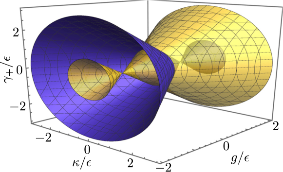
Figure 1: Two doubled cones with the shared axis defined by $\kappa/\epsilon=\gamma_{+}/\epsilon=0$ identify the positions of QEPs in the space spanned by the parameters $\gamma_{+}/\epsilon$, $\kappa/\epsilon$, and $g/\epsilon$. At $g/\epsilon=0$, the two cones intersect which gives rise to the QHPs whose positions form a circle. We note that the surfaces of QEPs are symmetric with respect to the plane $g/\epsilon=0$.

If $g=0$, two-fold degeneracy in eigenfrequencies occurs. Real nonzero eigenfrequencies $\Omega_{1,2}^{\rm r}$ exist only for $\epsilon^{2}-\kappa^{2}-\gamma_{+}^{2}>0$. When

$$\epsilon^{2}-\kappa^{2}-\gamma_{+}^{2}=0,$$ (93)

all the four eigenfrequencies coincide. They form doubly degenerate QEPs localized at a hypersurface of dimension 3 in the parameter space $(\gamma_{1}^{\rm d},\gamma_{2}^{\rm a},\epsilon,\kappa)$ defined by the condition in Eq. (93). The positions of the QEPs fulfilling Eq. (93) form the circle with radius 1 in the space of parameters $\gamma_{+}/\epsilon$ and $\kappa/\epsilon$ shown in Fig. 1 (the intersection of the yellow and blue cones). At these QEPs, there exist two different eigenvectors each arising from the original collapsing two dimensional spaces [46]. We have the QHPs in this case. We note that the nonclassical properties of optical fields generated at and around these QHPs were analyzed in [46] where even a more general Hamiltonian involving the additional Kerr nonlinear terms was considered.

Now let us have a deeper look at the eigenfrequencies and their spectral bifurcations that identify QEPs. To correctly identify QEPs, we also need to know the eigenvectors that correspond to the analyzed eigenfrequencies. The eigenvectors $Y_{1}$, $\bar{Y}_{1}$, $Y_{2}$, and $\bar{Y}_{2}$ given in Eq. (90), arising in the diagonalization of the dynamics matrix of the Heisenberg-Langevin equations (82), and belonging in turn to the eigenfrequencies $\Omega_{1}$, $-\Omega_{1}^{*}$, $\Omega_{2}$, and $-\Omega_{2}^{*}$, may be used to form the eigenvectors of the dynamics matrices of FOMs with increasing order. They directly represent the eigenvectors of the first-order FOMs dynamics matrix and, when formed into the supervector ${\cal Y}^{T}\equiv({\bf Y}_{1},\bar{\bf Y}_{1},{\bf Y}_{2},\bar{\bf Y}_{2})$, they allow to express the eigenvectors of the dynamics matrix of a $p$th-order FOMs via the tensor product $\underbrace{{\cal Y}\otimes\ldots\otimes{\cal Y}}_{p}$ [38]. This allows us, among other properties, to identify the number of eigenfrequencies for a given order of FOMs and their degeneracies occurring at QEPs.

The spectra of the eigenfrequencies and the numbers of eigenvectors differ in the above-discussed two cases ($g\neq 0$ and $g=0$). Whereas three independent eigenvectors of the dynamics matrix of the Heisenberg-Langevin equations occur at the QEPs for $g\neq 0$, only two of the eigenvectors are found at the QHPs when $g=0$. We note that, in both cases, all the eigenvalues contribute to the dynamics of the original field operators $\hat{a}_{1}$, $\hat{a}_{1}^{\dagger}$, $\hat{a}_{2}$, and $\hat{a}_{2}^{\dagger}$ and so the analysis of the evolution of any of them allows, in principle, to identify QEPs. In the following eigenfrequency analysis, we pay a detailed attention to the eigenfrequencies belonging to the FOMs up to the fourth order and draw some conclusions concerning general orders.

5.1 Spectra of eigenfrequencies for a single nondegenerate QEP

We first consider the case for $g\neq 0$, in which a single QEP with a double QEP degeneration occurs in the spectrum of the dynamics matrix of the Heisenberg-Langevin equations. At this QEP, three independent eigenvectors suffice in describing the system evolution. In general, the eigenfrequency analysis of the equations for the first-order FOMs provides four eigenfrequencies $\pm\Omega_{1,2}^{\rm r}-i\Omega^{\rm i}$. Two of them (say $\pm\Omega_{1}^{\rm r}-i\Omega^{\rm i}$) reveal the position of a QEP identified by the condition $\Omega_{1}^{\rm r}=0$.

This position of the QEP is also indicated by the eigenfrequencies originating in the analysis of higher-order FOMs. We have in turn 4, 16, 64, and 256 moments of the first, second, third, and fourth orders. However, as discussed above, some of these moments differ just in the positions of field operators. This means that they are either equal or differ by the moments of lower orders if the involved field operators do not commute. Taking into account this moment degeneracy, we may expect at maximum 4, 10, 20, and 35 different eigenfrequencies from the analysis of moments of the first, second, third, and fourth order. Degeneracy of the moments is given in Tables 1 and 2 for this case. This degeneracy is either mapped into the multiplicity of the corresponding QEPs (forming QHPs from QEPs and being characterized by a QDP degeneracy) or results in higher QEP degeneracies of QEPs (higher-order QEPs [36]). Whereas the moments $\langle\hat{b}_{1}\hat{b}_{2}\rangle$, $\langle\hat{b}_{2}\hat{b}_{1}\rangle$, $\langle\hat{b}_{1}^{\dagger}\hat{b}_{2}\rangle$, and $\langle\hat{b}_{2}\hat{b}_{1}^{\dagger}\rangle$ serve as examples in the former case, the moments $\langle\hat{b}_{1}^{\dagger}\hat{b}_{1}\rangle$ and $\langle\hat{b}_{1}\hat{b}_{1}^{\dagger}\rangle$ participate in forming a four-fold degenerated QEP (see Table 1). The eigenfrequencies attained by the analysis of the first-, second-, third- and fourth-order FOMs are summarized in Tables 1 and 2 depending on their ability to form QEPs. We note that some of the eigenfrequencies summarized in Table 2, that do not form QEPs, are degenerated, i.e. they exhibit QDP degeneracy.

Provided that $\Omega^{\rm i}\neq 0$, we observe in the spectra of eigenfrequencies in turn 1, 3, 6, and 10 bifurcations coming from the behavior of the first-, second-, third-, and fourth-order FOMs, as listed in Table 1. Following Table 1, there occur QHPs with QDP degeneracies 2, 6, and 12 considering in turn the moments of the second, third, and fourth order. On the other hand, the maximal QEP degeneracy of QEPs reached for the first-, second-, third-, and fourth-order FOMs equals 2, 4, 8 and 16. Here, we conclude that, in general, the analysis of $p$th-order FOMs gives QEPs with a $2^{p}$-fold degeneracy. We note that some eigenfrequencies remain single as seen in Table 2. In Tables 1 and 2, we mention, side by side with the eigenfrequencies, the corresponding moments of the ‘diagonalized’ field operators, as there is one-to-one mapping between these moments and the structure of the eigenfrequencies.

We note that, at the QEPs observed in the dynamics matrix of the Heisenberg-Langevin equations, the number of independent eigenvectors, given in Eq. (90), decreases from 4 to 3. This is so as two eigenvectors have to coalesce at a nondegenerate QEP. This results in the reduction of the complexity of the system dynamics and leads to all physical effects discussed in relation to QEPs. Considering higher-order FOMs, the number of independent eigenvectors arising from the dynamics matrix of $p$th-order FOMs decreases from $4^{p}$ to $3^{p}$, which also gives the maximal number of possibly different eigenfrequencies. Thus, the dynamics of higher-order field-operator correlation functions is more simplified at QEPs than that of the field mean operator amplitudes.

The eigenfrequencies that are related to the moments containing the ‘building block’ $\hat{b}_{1}^{\dagger}\hat{b}_{1}$ (e.g., the moments $\langle\hat{b}_{1}^{\dagger}\hat{b}_{1}\rangle$ and $\langle\hat{b}_{1}^{\dagger}\hat{b}_{1}\hat{b}_{2}\rangle$ in Table 1) form hidden QEPs. The contribution to the overall eigenfrequency of a higher-order FOM from this ‘building block’ equals zero as $\Omega_{1}^{\rm r}-\Omega_{1}^{\rm r}=0$ independently of whether there is a QEP or not. However, the presence of a QEP is identified by the reduction of the number of eigenvectors by one that happens in this case without any manifestation in the eigenfrequencies spectrum. Thus, no spectral bifurcation commonly used for identifying QEPs is observed. We note that, for the QEPs listed in Table 1, such eigenfrequencies form QEPs more than doubly degenerated, together with other eigenfrequencies, and so these QEPs are still identified in the spectrum by bifurcations.

In the usually discussed $\cal PT$-symmetric systems, gain and loss are in balance giving $\Omega^{\rm i}=0$. In this case, multiplicties (i.e., QDP degeneracies) of QEPs may even be higher as the imaginary parts of eigenfrequencies coming from different orders of FOMs coincide. For example, the QEPs positioned at $\pm\Omega_{1}^{\rm r}$ arise in the eigenfrequencies of both the first- and third-order FOMs, in the latter case even with QDP degeneracy 6 (see Table 1). Such QEPs are called genuine QEPs, as discussed below.

We note that, when describing the evolution of FOMs of a given order, we may neglect the redundant moments and keep just the differential equations for the remaining ones. The eigenfrequencies, originating in the analysis of such equations, remain the same as those analyzed above and summarized in Tables 1 and 2, but their multiplicities are just 1. Also, the reduction in the number of involved moments results in the change of the structure of the space of eigenvectors. This reduction conceals the QHPs identified in the last column of Table 1. We may call such QHPs as the induced QHPs as they originate in the extended space of FOMs that includes also the redundant moments. However, some QHPs, which we refer to as the genuine QHPs, still remain. These occur for $\Omega^{\rm i}=0$ and are formed by identical eigenfrequencies with different eigenvectors arising in the analysis of dynamics matrices for different orders FOMs (e.g., $\langle\hat{b}_{1}\rangle$ and $\langle\hat{b}_{1}^{\dagger}\rangle$ versus $\langle\hat{b}_{1}\hat{b}_{2}\hat{b}_{2}^{\dagger}\rangle$ and $\langle\hat{b}_{1}^{\dagger}\hat{b}_{2}^{\dagger}\hat{b}_{2}\rangle$).

We also note that when reducing the number of necessary FOMs of given order, we face the problem of non-commuting operators. However, the FOMs that contain non-commuting operators at different positions mutually differ by FOMs of orders lower by $2,4,6,\ldots$: Each application of nontrivial commutation relation reduced the moments order by two. When writing the differential equations for the set of FOMs of given order, we arrive at the equations similar to those found in Eqs. (61), (64) and (66) that, however, contain additional terms formed by lower-order FOMs at their r.h.s. Nevertheless, these terms modify the nonhomogeneous solution of the equations qualitatively in the same way as those arising in the fluctuating Langevin forces, i.e. the solution is enriched by the terms oscillating at the eigenfrequencies appropriate to these lower-order FOMs. Thus the terms arising from the non-commuting operators do not change the eigenfrequencies and we may apply the above results concerning the eigenfrequencies also in this case. On the other hand, the eigenvectors in both approaches naturally differ. Their mutual relations [47] were discussed in relation to the quantum versus classical descriptions in [38].

${\bf\Omega^{\rm i}_{\rm gen}}$	${\bf\Omega^{\rm r}_{\rm gen}}$	Moments	QDP deg.
$\Omega^{\rm i}$	$\Omega_{2}^{\rm r}$	$\langle\hat{b}_{2}\rangle$	1
	$-\Omega_{2}^{\rm r}$	$\langle\hat{b}_{2}^{\dagger}\rangle$	1
$2\Omega^{\rm i}$	0	$\langle\hat{b}_{2}^{\dagger}\hat{b}_{2}\rangle$	2
	$2\Omega_{2}^{\rm r}$	$\langle\hat{b}_{2}^{2}\rangle$	1
	$-2\Omega_{2}^{\rm r}$	$\langle\hat{b}_{2}^{\dagger 2}\rangle$	1
$3\Omega^{\rm i}$	$\Omega_{2}^{\rm r}$	$\langle\hat{b}_{2}^{\dagger 2}\hat{b}_{2}\rangle$	3
	$-\Omega_{2}^{\rm r}$	$\langle\hat{b}_{2}^{\dagger}\hat{b}_{2}^{2}\rangle$	3
	$3\Omega_{2}^{\rm r}$	$\langle\hat{b}_{2}^{3}\rangle$	1
	$-3\Omega_{2}^{\rm r}$	$\langle\hat{b}_{2}^{\dagger 3}\rangle$	1
$4\Omega^{\rm i}$	0	$\langle\hat{b}_{2}^{\dagger 2}\hat{b}_{2}^{2}\rangle$	6
	$2\Omega_{2}^{\rm r}$	$\langle\hat{b}_{2}^{\dagger}\hat{b}_{2}^{3}\rangle$	4
	$-2\Omega_{2}^{\rm r}$	$\langle\hat{b}_{2}^{\dagger 3}\hat{b}_{2}\rangle$	4
	$4\Omega_{2}^{\rm r}$	$\langle\hat{b}_{2}^{4}\rangle$	1
	$-4\Omega_{2}^{\rm r}$	$\langle\hat{b}_{2}^{\dagger 4}\rangle$	1

Table 2: Real and imaginary parts of the complex eigenfrequencies $\Omega_{\rm gen}^{\rm r}-i\Omega_{\rm gen}^{\rm i}$ derived from the equations for the FOMs up to fourth order which do not indicate a QEP for $g\neq 0$. The corresponding moments in the ‘diagonalized’ field operators are written together with their QDP degeneracies resulting from different orderings of field operators.

5.2 Spectra of eigenfrequencies for a doubly degenerated QEP - QHP

The squeezing-effect part of the Hamiltonian $\hat{H}^{0}$ in Eq. (69) is often not considered ($g=0$). This leads to two doubly degenerated eigenfrequencies $\pm\Omega^{\rm r}-i\Omega^{\rm i}$, when the dynamics of the first-order FOMs is investigated. They form a QHP occurring directly in the dynamics matrix of the Heisenberg-Langevin equations. This QDP degeneracy is then directly transformed into the diabolical degeneracies of eigenfrequencies arising from the analysis of higher-order FOMs. We may call such QHP the inherited QHP. This inherited QDP degeneracy considerably reduces the number of different spectral eigenfrequencies provided by higher-order FOMs, at the expense of their increasing degeneracies. We note that this behavior was observed in [21], where the spectrum of the Liouvillian of a simplified two-mode bosonic system with $g=\kappa=0$ was numerically analyzed. The obtained eigenfrequencies, their QDP and QEP degeneracies and the corresponding QHPs are summarized in Table 3, together with the corresponding ‘diagonalized’ FOMs.

${\bf\Omega^{\rm i}_{\rm gen}}$	${\bf\Omega^{\rm r}_{\rm gen}}$	Moments	Moment	Partial	Partial
			deg.	QDP x	QDP x
				QEP deg.	QEP deg.
$\Omega^{\rm i}$	$\pm\Omega^{\rm r}$	$\langle\hat{b}_{1}\rangle$, $\langle\hat{b}_{1}^{\dagger}\rangle$	1	1x2	2x2
		$\langle\hat{b}_{2}\rangle$, $\langle\hat{b}_{2}^{\dagger}\rangle$	1	1x2
$2\Omega^{\rm i}$	$\pm 2\Omega^{\rm r}$	$\langle\hat{b}_{1}\hat{b}_{2}\rangle$, $\langle\hat{b}_{1}^{\dagger}\hat{b}_{2}^{\dagger}\rangle$	2	2x4	4x4
	$\Omega^{\rm r}-\Omega^{\rm r}$	$\langle\hat{b}_{1}^{\dagger}\hat{b}_{2}\rangle$	2
	$\Omega^{\rm r}-\Omega^{\rm r}$	$\langle\hat{b}_{1}\hat{b}_{2}^{\dagger}\rangle$	2
	$\pm 2\Omega^{\rm r}$	$\langle\hat{b}_{1}^{2}\rangle$, $\langle\hat{b}_{1}^{\dagger 2}\rangle$	1	1x4
	$\Omega^{\rm r}-\Omega^{\rm r}$	$\langle\hat{b}_{1}^{\dagger}\hat{b}_{1}\rangle$	2
	$\pm 2\Omega^{\rm r}$	$\langle\hat{b}_{2}^{2}\rangle$, $\langle\hat{b}_{2}^{\dagger 2}\rangle$	1	1x4
	$\Omega^{\rm r}-\Omega^{\rm r}$	$\langle\hat{b}_{2}^{\dagger}\hat{b}_{2}\rangle$	2
$3\Omega^{\rm i}$	$\pm 3\Omega^{\rm r}$	$\langle\hat{b}_{1}^{2}\hat{b}_{2}\rangle$, $\langle\hat{b}_{1}^{\dagger 2}\hat{b}_{2}^{\dagger}\rangle$	3	3x8	8x8
	$\pm\Omega^{\rm r}$	$\langle\hat{b}_{1}^{2}\hat{b}_{2}^{\dagger}\rangle$, $\langle\hat{b}_{1}^{\dagger 2}\hat{b}_{2}\rangle$	3
		$\langle\hat{b}_{1}^{\dagger}\hat{b}_{1}\hat{b}_{2}\rangle$, $\langle\hat{b}_{1}^{\dagger}\hat{b}_{1}\hat{b}_{2}^{\dagger}\rangle$	6
	$\pm 3\Omega^{\rm r}$	$\langle\hat{b}_{1}\hat{b}_{2}^{2}\rangle$, $\langle\hat{b}_{1}^{\dagger}\hat{b}_{2}^{\dagger 2}\rangle$	3	3x8
	$\pm\Omega^{\rm r}$	$\langle\hat{b}_{1}^{\dagger}\hat{b}_{2}^{2}\rangle$, $\langle\hat{b}_{1}\hat{b}_{2}^{\dagger 2}\rangle$	3
		$\langle\hat{b}_{1}\hat{b}_{2}^{\dagger}\hat{b}_{2}\rangle$, $\langle\hat{b}_{1}^{\dagger}\hat{b}_{2}^{\dagger}\hat{b}_{2}\rangle$	6
	$\pm 3\Omega^{\rm r}$	$\langle\hat{b}_{1}^{3}\rangle$, $\langle\hat{b}_{1}^{\dagger 3}\rangle$	1	1x8
	$\pm\Omega^{\rm r}$	$\langle\hat{b}_{1}^{\dagger}\hat{b}_{1}^{2}\rangle$, $\langle\hat{b}_{1}^{\dagger 2}\hat{b}_{1}\rangle$	3
	$\pm 3\Omega^{\rm r}$	$\langle\hat{b}_{2}^{3}\rangle$, $\langle\hat{b}_{2}^{\dagger 3}\rangle$	1	1x8
	$\pm\Omega^{\rm r}$	$\langle\hat{b}_{2}^{\dagger}\hat{b}_{2}^{2}\rangle$, $\langle\hat{b}_{2}^{\dagger 2}\hat{b}_{2}\rangle$	3
$4\Omega^{\rm i}$	$\pm 4\Omega^{\rm r}$	$\langle\hat{b}_{1}^{3}\hat{b}_{2}\rangle$, $\langle\hat{b}_{1}^{\dagger 3}\hat{b}_{2}^{\dagger}\rangle$	4	4x16	16x16
	$\pm 2\Omega^{\rm r}$	$\langle\hat{b}_{1}^{3}\hat{b}_{2}^{\dagger}\rangle$, $\langle\hat{b}_{1}^{\dagger 3}\hat{b}_{2}\rangle$	4
		$\langle\hat{b}_{1}^{\dagger}\hat{b}_{1}^{2}\hat{b}_{2}\rangle$, $\langle\hat{b}_{1}\hat{b}_{1}^{\dagger 2}\hat{b}_{2}^{\dagger}\rangle$	12
	$2\Omega^{\rm r}-2\Omega^{\rm r}$	$\langle\hat{b}_{1}^{\dagger}\hat{b}_{1}^{2}\hat{b}_{2}^{\dagger}\rangle$ , $\langle\hat{b}_{1}^{\dagger 2}\hat{b}_{1}\hat{b}_{2}\rangle$	12
	$\pm 4\Omega^{\rm r}$	$\langle\hat{b}_{1}\hat{b}_{2}^{3}\rangle$, $\langle\hat{b}_{1}^{\dagger}\hat{b}_{2}^{\dagger 3}\rangle$	4	4x16
	$\pm 2\Omega^{\rm r}$	$\langle\hat{b}_{1}^{\dagger}\hat{b}_{2}^{3}\rangle$, $\langle\hat{b}_{1}\hat{b}_{2}^{\dagger 3}\rangle$	4
		$\langle\hat{b}_{1}\hat{b}_{2}^{\dagger}\hat{b}_{2}^{2}\rangle$, $\langle\hat{b}_{1}^{\dagger}\hat{b}_{2}^{\dagger 2}\hat{b}_{2}\rangle$	12
	$2\Omega^{\rm r}-2\Omega^{\rm r}$	$\langle\hat{b}_{1}\hat{b}_{2}^{\dagger 2}\hat{b}_{2}\rangle$ , $\langle\hat{b}_{1}^{\dagger}\hat{b}_{2}^{2}\hat{b}_{2}^{\dagger}\rangle$	12
	$\pm 4\Omega^{\rm r}$	$\langle\hat{b}_{1}^{2}\hat{b}_{2}^{2}\rangle$, $\langle\hat{b}_{1}^{\dagger 2}\hat{b}_{2}^{\dagger 2}\rangle$	6	6x16
	$2\Omega^{\rm r}-2\Omega^{\rm r}$	$\langle\hat{b}_{1}^{2}\hat{b}_{2}^{\dagger 2}\rangle$, $\langle\hat{b}_{1}^{\dagger 2}\hat{b}_{2}^{2}\rangle$	6
	$\pm 2\Omega^{\rm r}$	$\langle\hat{b}_{1}^{2}\hat{b}_{2}^{\dagger}\hat{b}_{2}\rangle$, $\langle\hat{b}_{1}^{\dagger 2}\hat{b}_{2}^{\dagger}\hat{b}_{2}\rangle$	12
		$\langle\hat{b}_{1}^{\dagger}\hat{b}_{1}\hat{b}_{2}^{2}\rangle$, $\langle\hat{b}_{1}^{\dagger}\hat{b}_{1}\hat{b}_{2}^{\dagger 2}\rangle$	12
	$2\Omega^{\rm r}-2\Omega^{\rm r}$	$\langle\hat{b}_{1}^{\dagger}\hat{b}_{1}\hat{b}_{2}^{\dagger}\hat{b}_{2}\rangle$	24
	$\pm 4\Omega^{\rm r}$	$\langle\hat{b}_{1}^{4}\rangle$, $\langle\hat{b}_{1}^{\dagger 4}\rangle$	1	1x16
	$\pm 2\Omega^{\rm r}$	$\langle\hat{b}_{1}^{\dagger}\hat{b}_{1}^{3}\rangle$, $\langle\hat{b}_{1}^{\dagger 3}\hat{b}_{1}\rangle$	4
	$2\Omega^{\rm r}-2\Omega^{\rm r}$	$\langle\hat{b}_{1}^{\dagger 2}\hat{b}_{1}^{2}\rangle$	6
	$\pm 4\Omega^{\rm r}$	$\langle\hat{b}_{2}^{4}\rangle$, $\langle\hat{b}_{2}^{\dagger 4}\rangle$	1	1x16
	$\pm 2\Omega^{\rm r}$	$\langle\hat{b}_{2}^{\dagger}\hat{b}_{2}^{3}\rangle$, $\langle\hat{b}_{2}^{\dagger 3}\hat{b}_{2}\rangle$	4
	$2\Omega^{\rm r}-2\Omega^{\rm r}$	$\langle\hat{b}_{2}^{\dagger 2}\hat{b}_{2}^{2}\rangle$	6

Table 3: Real and imaginary parts of the complex eigenfrequencies $\Omega_{\rm gen}^{\rm r}-i\Omega_{\rm gen}^{\rm i}$ derived from the equations for the FOMs up to fourth order which indicate a QHP for $g=0$. The corresponding moments in the ‘diagonalized’ field operators are written together with their degeneracies coming from different orderings of field operators. QDP degeneracies of QHPs (partial QDP degeneracies) derived from the indicated FOMs and QEP degeneracies of the constituting QEPs are given.

According to Table 3, the QEPs found for the dynamics matrix of $p$th-order FOMs exhibit a $2^{p}$-fold QEP degeneracy. Due to the inherited spectral degeneracy, the frequencies of all QEPs belonging to $p$th-order FOMs equal zero ($\Omega^{\rm r}=0$), which results in the occurrence of the QHP with a QDP degeneracy $2^{p}$ formed by $2^{p}$ QEPs with a $2^{p}$-fold QEP degeneracy, as shown in Table 3. This results from the fact that the number of independent eigenvectors of the dynamics matrix of the Heisenberg-Langevin equations decreases from 4 to 2 at QHPs.

As seen in Table 3, we have the hidden QEPs/QHPs also in this case. They occur not only in relation to the moments of a single mode (e.g., $\langle\hat{b}_{1}^{\dagger}\hat{b}_{1}\rangle$ and $\langle\hat{b}_{1}\hat{b}_{1}^{\dagger}\rangle$), but also when cross moments of different modes are considered (e.g., $\langle\hat{b}_{1}^{\dagger}\hat{b}_{2}\rangle$ and $\langle\hat{b}_{1}\hat{b}_{2}^{\dagger}\rangle$, or $\langle\hat{b}_{2}\hat{b}_{1}^{\dagger}\rangle$ and $\langle\hat{b}_{2}^{\dagger}\hat{b}_{1}\rangle$). Apart from the hidden QEPs, we observe spectral bifurcations at $\pm p\Omega^{\rm r}$, $\pm(p-2)\Omega^{\rm r}$, $\pm(p-4)\Omega^{\rm r}$, $\ldots$ from the $p$th-order FOMs.

Provided that we exclude the redundant FOMs from the description, the QDP degeneracy of QHPs identified in Table 3, in general, lowers. Whereas it remains 2 for the first-order FOMs, it decreases from $2^{p}$ to $p+1$ for $p$th-order FOMs.

Finally, we discuss some properties of eigenfrequencies when the FOMs of all orders are considered. Provided that the gain and loss are in balance, we have ${\Omega}^{\rm i}=0$ and we can directly compare the eigenfrequencies arising in the dynamics matrices of FOMs of different orders. Then the QEPs are localized with the help of pairs of eigenfrequencies $\pm p\Omega_{1}^{\rm r}$ ($g\neq 0$) and $\pm p\Omega^{\rm r}$ ($g=0$) for $p=1,2,\ldots$ occurring infinitely-many times in the spectrum. For $g\neq 0$, the other pairs of eigenfrequencies, as explicitly written in Table 1, are, among others, also found in the spectrum with infinite degeneration.

At the end, we note that, when the eigenfrequency analysis is accompanied by the determination of the corresponding eigenvectors, we can discuss the modes behavior at a general level using the quantities based on the determined FOMs. For example, phase squeezing is revealed by the behavior of the second-order FOMs [33, 48], whereas sub-Poissonian photon-number statistics [34] of the modes and their sub-shot-noise photon-number correlations [49] are quantified by the fourth-order FOMs. Also different types of nonclassicalities can be discussed [50].

We also note that our approach relies on the linear Heisenberg-Langevin equations. Nevertheless, it may be successfully applied also in investigations of quantum systems described by the nonlinear Heisenberg-Langevin equations provided that a suitable operator linearization of the nonlinear operator equations is applied, e.g. around a stationary state or a classical time-dependent solution [46, 51, 52, 53].

6 Conclusions

We have shown that the eigenfrequency analysis of the Liouvillians of open quantum systems can alternatively be performed in the space of operators of measurable quantities provided that they form a complete basis. This is especially important for systems defined in infinite-dimensional Liouville spaces including those formed by the interacting bosonic fields. Considering a damped two-level atom, we have demonstrated the equivalence of both approaches in obtaining the system eigenfrequencies and positions of quantum exceptional points. Analysing the dynamical equations of field-operator moments of general $M$-mode fields, we have revealed the structure of eigenfrequencies attainable from dynamical equations for a given order of the field-operator moments. This shed light to the occurrence of quantum exceptional points identified from the obtained eigenfrequencies: All quantum exceptional points are recognized already from the eigenfrequencies obtained from the first-order field-operator moments. The eigenfrequencies obtained from higher-order field-operator moments are important in revealing multiple (i.e., diabolical) degeneracies of these quantum exceptional points only. We have developed a general approach to analyze a two-mode bosonic system described by a general quadratic Hamiltonian. In its general configuration, two distinct sets of quantum exceptional points occur for nonzero mode squeezing that, however, collapse into a single set with quantum hybrid diabolical exceptional points, when mode squeezing is not considered. In the analysis, we have observed the inherited, genuine and induced quantum hybrid diabolical exceptional points. Moreover, the hidden quantum exceptional points, whose presence is not directly inferred from the behavior of eigenfrequency spectra, were identified.

The consideration of the Heisenberg-Langevin equations for the operators of measurable quantities and the derived dynamical equations for field-operator moments represent a convenient starting point for the system eigenfrequency analysis that allows to reveal the eigenfrequencies of open quantum systems encoded in their Liouvillians. We believe that this approach is qualitatively less demanding compared to a direct diagonalization of the Liouvillians, at least when the linear Heisenberg-Langevin equations describe the analyzed system. This approach paves the way to a general and detailed analysis of quantum exceptional points in open quantum infinitely-dimensional systems.

References

• [1] C. M. Bender and S. Boettcher. “Real spectra in non-Hermitian Hamiltonians having $\mathcal{PT}$ symmetry”. Phys. Rev. Lett. 80, 5243–5246 (1998).
• [2] C. M. Bender, D. C. Brody, and H. F. Jones. “Must a Hamiltonian be Hermitian?”. Am. J. Phys. 71, 1095–1102 (2003).
• [3] C. M. Bender. “Making sense of non-Hermitian Hamiltonians”. Reports Progress Phys. 70, 947 (2007).
• [4] R. El-Ganainy, K. G. Makris, M. Khajavikhan, Z. H. Musslimani, S. Rotter, and D. N. Christodoulides. “Non-Hermitian physics and $\mathcal{PT}$ symmetry”. Nat. Phys. 14, 11 (2018).
• [5] Y. Ashida, Z. Gong, and M. Ueda. “Non-Hermitian physics”. Adv. Phys. 69, 249 (2020).
• [6] A. Mostafazadeh. “Pseudo-Hermiticity and generalized $\mathcal{PT}$ and $\mathcal{CPT}$-symmetries”. J. Math. Phys. (Melville, NY) 44, 974 (2003).
• [7] A. Mostafazadeh. “Time dependent Hilbert spaces, geometric phases, and general covariance in quantum mechanics”. Phys. Lett. A 320, 375 (2004).
• [8] A. Mostafazadeh. “Pseudo-Hermitian representation of quantum mechanics”. Int. J. Geom. Methods Mod. Phys. 7, 1191 (2010).
• [9] M. Znojil. “Time-dependent version of crypto-Hermitian quantum theory”. Phys. Rev. D 78, 085003 (2008).
• [10] D. C. Brody. “Biorthogonal quantum mechanics”. J. Phys. A: Math. Theor. 47, 035305 (2014).
• [11] F. Bagarello, R. Passante, and C. Trapani. “Non-Hermitian Hamiltonians in quantum physics”. In Non-Hermitian Hamiltonians in Quantum Physics. Springer, New York (2016).
• [12] L. Feng, R. El-Ganainy, and L. Ge. “Non-Hermitian photonics based on parity-time symmetry”. Nat. Photon. 11, 752 (2017).
• [13] R. El-Ganainy, M. Khajavikhan, D. N. Christodoulides, and Ş. K. Özdemir. “The dawn of non-Hermitian optics”. Commun. Phys. 2, 1 (2019).
• [14] M. Parto, Y. G. N. Liu, B. Bahari, M. Khajavikhan, and D. N. Christodoulides. “Non-Hermitian and topological photonics: optics at an exceptional point”. Nanophotonics 10, 403 (2021).
• [15] Ch.-Y. Ju, A. Miranowicz, F. Minganti, C.-Ts. Chan, G.-Y. Chen, and F. Nori. “Flattening the curve with Einstein’s quantum elevator: Hermitization of Non-Hermitian Hamiltonians via the vielbein formalism”. Phys. Rev. Research 4, 023070 (2022).
• [16] M. Znojil. “Is $\mathcal{PT}$-symmetric quantum theory false as a fundamental theory?”. Acta Polytech. 56, 254 (2016).
• [17] C.-Y. Ju, A. Miranowicz, G.-Y. Chen, and F. Nori. “Non-Hermitian Hamiltonians and no-go theorems in quantum information”. Phys. Rev. A 100, 062118 (2019).
• [18] C. M. Bender, D. C. Brody, and M. P. Müller. “Hamiltonian for the zeros of the Riemann Zeta function”. Phys. Rev. Lett. 118, 130201 (2017).
• [19] Ş. K. Özdemir, S. Rotter, F. Nori, and L. Yang. “Parity–time symmetry and exceptional points in photonics”. Nat. Mater. 18, 783 (2019).
• [20] M.-A. Miri and A. Alù. “Exceptional points in optics and photonics”. Science 363, eaar7709 (2019).
• [21] F. Minganti, A. Miranowicz, R. Chhajlany, and F. Nori. “Quantum exceptional points of non-Hermitian Hamiltonians and Liouvillians: The effects of quantum jumps”. Phys. Rev. A 100, 062131 (2019).
• [22] H. J. Carmichael. “Quantum trajectory theory for cascaded open systems”. Phys. Rev. Lett. 70, 2273 (1993).
• [23] J. Dalibard, Y. Castin, and K. Mølmer. “Wave-function approach to dissipative processes in quantum optics”. Phys. Rev. Lett. 68, 580 (1992).
• [24] K. Mølmer, Y. Castin, and J. Dalibard. “Monte Carlo wavefunction method in quantum optics”. J. Opt. Soc. Am. B 10, 524 (1993).
• [25] M. B. Plenio and P. L. Knight. “The quantum-jump approach to dissipative dynamics in quantum optics”. Rev. Mod. Phys. 70, 101 (1998).
• [26] H. Breuer and F. Petruccione. “The theory of open quantum systems”. Oxford University Press, Oxford.  (2007).
• [27] J. Gunderson, J. Muldoon, K. W. Murch, and Y. N. Joglekar. “Floquet exceptional contours in Lindblad dynamics with time-periodic drive and dissipation”. Phys. Rev. A 103, 023718 (2021).
• [28] W. Chen, M. Abbasi, B. Ha, S. Erdamar, Y. N. Joglekar, and K. W. Murch. “Decoherence induced exceptional points in a dissipative superconducting qubit”. Phys. Rev. Lett. 128, 110402 (2022).
• [29] M. Naghiloo, M. Abbasi, Y. N. Joglekar, and K. W. Murch. “Quantum state tomography across the exceptional point in a single dissipative qubit”. Nat. Phys. 15, 1232 (2019).
• [30] F. Minganti, A. Miranowicz, R. W. Chhajlany, I. I. Arkhipov, and F. Nori. “Hybrid-Liouvillian formalism connecting exceptional points of non-Hermitian Hamiltonians and Liouvillians via postselection of quantum trajectories”. Phys. Rev. A 101, 062112 (2020).
• [31] F. Minganti, I. I. Arkhipov, A. Miranowicz, and F. Nori. “Liouvillian spectral collapse in the Scully-Lamb laser model”. Phys. Rev. Research 3, 043197 (2021).
• [32] F. Minganti, I. I. Arkhipov, A. Miranowicz, and F. Nori. “Continuous dissipative phase transitions with or without symmetry breaking”. New J. Phys. 23, 122001 (2021).
• [33] A. Lukš, V. Peřinová, and J. Peřina. “Principal squeezing of vacuum fluctuations”. Opt. Commun. 67, 149—151 (1988).
• [34] L. Mandel and E. Wolf. “Optical coherence and quantum optics”. Cambridge Univ. Press, Cambridge.  (1995).
• [35] J. Peřina. “Quantum statistics of linear and nonlinear optical phenomena”. Kluwer, Dordrecht.  (1991).
• [36] I. I. Arkhipov, F. Minganti, A. Miranowicz, and F. Nori. “Generating high-order quantum exceptional points in synthetic dimensions”. Phys. Rev. A 101, 012205 (2021).
• [37] I. I. Arkhipov and F. Minganti. “Emergent non-Hermitian skin effect in the synthetic space of (anti-)$\mathcal{PT}$-symmetric dimers” (2021).
• [38] I. I. Arkhipov, A. Miranowicz, F. Nori, S. K. Özdemir, and F. Minganti. “Geometry of the field-moment spaces for quadratic bosonic systems: Diabolically degenerated exceptional points on complex $k$-polytopes” (2022).
• [39] H. Mori. “Transport, collective motion, and Brownian motion”. Progr. Theor. Phys. 33, 423—445 (1965).
• [40] M. Tokuyama and H. Mori. “Statistical-mechanical theory of random frequency modulations and generalized Brownian motions”. Progr. Theor. Phys. 55, 411—429 (1976).
• [41] J. Peřina Jr. “On the equivalence of some projection operator techniques”. Physica A 214, 309—318 (1995).
• [42] W. Vogel and D. G. Welsch. “Quantum optics, 3rd ed.”. Wiley-VCH, Weinheim.  (2006).
• [43] P. Meystre and M. Sargent III. “Elements of quantum optics, 4nd edition”. Springer, Berlin.  (2007).
• [44] J. Peřina. “Coherence of light”. Kluwer, Dordrecht.  (1985).
• [45] I. I. Arkhipov, A. Miranowicz, F. Minganti, and F. Nori. “Quantum and semiclassical exceptional points of a linear system of coupled cavities with losses and gain within the Scully-Lamb laser theory”. Phys. Rev. A 101, 013812 (2020).
• [46] J. Peřina Jr., A. Lukš, J. K. Kalaga, W. Leoński, and A. Miranowicz. “Nonclassical light at exceptional points of a quantum $\mathcal{PT}$-symmetric two-mode system”. Phys. Rev. A 100, 053820 (2019).
• [47] Z. Hu. “Eigenvalues and eigenvectors of a class of irreducible tridiagonal matrices”. Linear Algebra Its Appl. 619, 328—337 (2015).
• [48] A. I. Lvovsky and M. G. Raymer. “Continuous-variable optical quantum state tomography”. Rev. Mod. Phys. 81, 299—332 (2009).
• [49] M. Bondani, A. Allevi, G. Zambra, M. G. A. Paris, and A. Andreoni. “Sub-shot-noise photon-number correlation in a mesoscopic twin beam of light”. Phys. Rev. A 76, 013833 (2007).
• [50] J. Peřina Jr., P. Pavlíček, V. Michálek, R. Machulka, and O. Haderka. “Nonclassicality criteria for N-dimensional optical fields detected by quadratic detectors”. Phys. Rev. A 105, 013706 (2022).
• [51] J. Peřina Jr. and A. Lukš. “Quantum behavior of a $\mathcal{PT}$-symmetric two-mode system with cross-Kerr nonlinearity”. Symmetry 11, 1020 (2019).
• [52] J. Peřina Jr. “Coherent light in intense spatiospectral twin beams”. Phys. Rev. A 93, 063857 (2016).
• [53] J. Peřina Jr. and J. Peřina. “Quantum statistics of nonlinear optical couplers”. In E. Wolf, editor, Progress in Optics, Vol. 41. Pages 361—419. Elsevier, Amsterdam (2000).
• [54] R. J. Glauber. “Coherent and incoherent states of the radiation field”. Phys. Rev. 131, 2766—2788 (1963).
• [55] E. C. G. Sudarshan. “Equivalence of semiclassical and quantum mechanical descriptions of statistical light beams”. Phys. Rev. Lett. 10, 277—179 (1963).
• [56] H. Risken. “The Fokker-Planck equation”. Springer, Berlin.  (1996).