Supplementary Material
GO-Surf: Neural Feature Grid Optimization for
Fast, High-Fidelity RGB-D Surface Reconstruction

1 Second-order Grid Sampler

In this section we provide additional details on our implementation of grid sampler that allows double back-propagation in PyTorch. As described in our main paper, thepredicted SDF value $\phi$ is a function of 3D coordinates of the query point $\mathbf{x}$, feature vectors in feature grid $\theta$, and geometry network parameters $\omega$:

$$\phi(\mathbf{x},\theta,\omega)=f_{\omega}(\mathbf{z}(\theta,\mathbf{x}))$$ (1)

where $\mathbf{z}=\mathcal{V}_{\theta}(\mathbf{x})\in\mathbb{R}^{C}$ is the tri-linearly interpolated feature vector at the query point $\mathbf{x}.$ The first-order gradient of the SDF w.r.t. 3D query coordinates is:

$$\frac{\partial\phi}{\partial\mathbf{x}} = \frac{\partial f_{\omega}(\mathbf{z})}{\partial\mathbf{z}}\frac{\partial\mathbf{z}}{\partial\mathbf{x}}$$ (2)

$$= \sum_{i=1}^{C}\frac{\partial f_{\omega}(\mathbf{z})}{\partial z_{i}}\frac{\partial z_{i}}{\partial\mathbf{x}}$$

Here, to avoid the usage of higher-order tensors in derivation of second-order derivatives we consider the derivatives for each individual feature dimension $z_{i}$, as in Eq. 2. To regularise this gradient term we need to obtain the gradient Eq. 2 w.r.t. $\mathbf{x}$, $\theta$ and $\omega$ respectively, which corresponds to the first three row of the Hessian of SDF:

$$\frac{\partial^{2}\phi}{\partial\mathbf{x}^{2}} = \sum_{i=1}^{C}\frac{\partial^{2}f_{\omega}(\mathbf{z})}{\partial z^{2}_{i}}\bigg{(}\frac{\partial z_{i}}{\partial\mathbf{x}}\bigg{)}^{2}+\frac{\partial f_{\omega}(\mathbf{z})}{\partial z_{i}}\frac{\partial^{2}z_{i}}{\partial\mathbf{x}^{2}}$$ (3)

$$\frac{\partial^{2}\phi}{\partial\mathbf{x}\partial\theta} = \sum_{i=1}^{C}\frac{\partial^{2}f_{\omega}(\mathbf{z})}{\partial z^{2}_{i}}\frac{\partial z_{i}}{\partial\mathbf{\theta}}\frac{\partial z_{i}}{\partial\mathbf{x}}+\frac{\partial f_{\omega}(\mathbf{z})}{\partial z_{i}}\frac{\partial^{2}z_{i}}{\partial\mathbf{x}\partial\theta}$$ (4)

$$\frac{\partial^{2}\phi}{\partial\mathbf{x}\partial\omega} = \sum_{i=1}^{C}\frac{\partial^{2}f_{\omega}(\mathbf{z})}{\partial z_{i}\partial\omega}\frac{\partial z_{i}}{\partial\mathbf{x}}$$ (5)

We don’t need to implement Eq. 5 as Pytorch’s automatic differentiation package supports double back-propagation through an MLP and Pytorch’s grid_sampler also has first-order gradient implementation. However Eq. 3 and  4 need to be implemented as they require double back-propagation through the grid_sampler which is not implemented in PyTorch.

Derivative Derivation.

Now we will derive the second-order derivatives of the tri-linear interpolation. More specifically, we only need two Hessian blocks: $\frac{\partial^{2}z_{i}}{\partial\mathbf{x}^{2}}$ and $\frac{\partial^{2}z_{i}}{\partial\mathbf{x}\partial\theta}$. For simplicity we derive with $1\text{-D}$ features, but it generalises to any feature dimensions as the derivation is equivalent to all dimensions. Assume we have a query point $\mathbf{x}=[x,y,z]$ and $8$ feature vectors (points) stacking in a column $\theta=[\theta_{000},\theta_{001},\theta_{010},\theta_{011},\theta_{100},\theta_{101},\theta_{110},\theta_{111}]^{T}\in\mathbb{R}^{8}$ that correspond to the eight vertices of the voxel that encloses the point $\mathbf{x}$. Then, the tri-linearly interpolated feature $f$ at point $\mathbf{x}$ is given by:

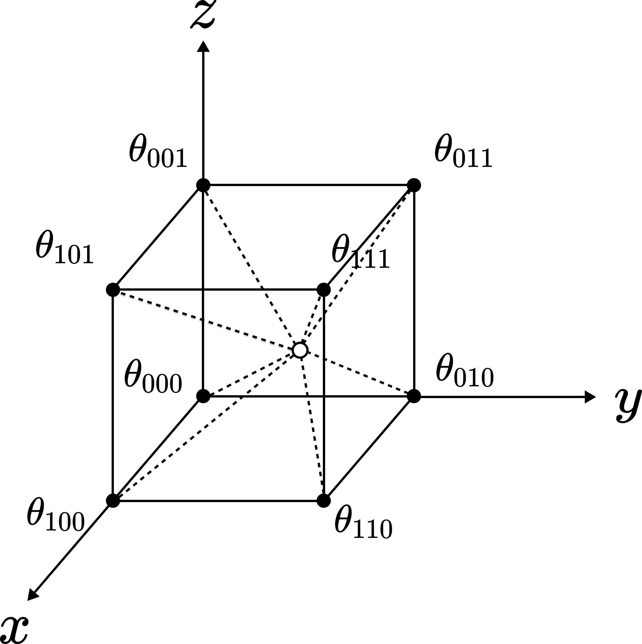
Figure 1: Example of trilinear interpolation in a 3D voxel.

$$f=\theta^{T}\mathbf{w}(\mathbf{x})$$ (6)

where $\mathbf{w}(\mathbf{x})\in\mathbb{R}^{8}$ is the coefficient vector of the 8 vertices:

$$\mathbf{w}(\mathbf{x})=\begin{bmatrix}(1-x)(1-y)(1-z)\\ (1-x)(1-y)z\\ (1-x)y(1-z)\\ (1-x)yz\\ x(1-y)(1-z)\\ x(1-y)z\\ xy(1-z)\\ xyz\\ \end{bmatrix}$$ (7)

Then the Jacobian of $f$ w.r.t. $\mathbf{x}$ is given by:

$$\frac{\partial f}{\partial\mathbf{x}}=\theta^{T}\frac{\partial\mathbf{w}(\mathbf{x})}{\partial\mathbf{x}}$$ (8)

where the Jacobian of the coefficient vector $\mathbf{w}$ w.r.t. query point $\mathbf{x}$ is a $8\times 3$ matrix and is given by:

$$\frac{\partial\mathbf{w}}{\partial\mathbf{x}} = \begin{bmatrix}\mathbf{J}_{1}&\mathbf{J}_{2}&\mathbf{J}_{3}\end{bmatrix}$$ (9)

$$\mathbf{J}_{1} = \begin{bmatrix}-(1-y)(1-z)\\ -(1-y)z\\ -y(1-z)\\ -yz\\ (1-y)(1-z)\\ (1-y)z\\ y(1-z)\\ yz\\ \end{bmatrix}$$ (10)

$$\mathbf{J}_{2} = \begin{bmatrix}-(1-x)(1-z)\\ -(1-x)z\\ (1-x)(1-z)\\ (1-x)z\\ -x(1-z)\\ -xz\\ x(1-z)\\ xz\\ \end{bmatrix}$$ (11)

$$\mathbf{J}_{3} = \begin{bmatrix}-(1-x)(1-y)\\ (1-x)(1-y)\\ -(1-x)y)\\ (1-x)y\\ -x(1-y)\\ x(1-y)\\ -xy\\ xy\\ \end{bmatrix}$$ (12)

Then the second-order derivative $\frac{\partial^{2}f}{\partial\mathbf{x}\partial\theta}$ is given by:

$$\frac{\partial^{2}f}{\partial\mathbf{x}\partial\mathbf{\theta}} = \frac{\partial}{\partial\theta}\bigg{(}\frac{\partial f}{\partial\mathbf{x}^{T}}\bigg{)}$$ (13)

$$= \bigg{(}\frac{\partial\mathbf{w}}{\partial\mathbf{x}}\bigg{)}^{T}$$

which is simply the transpose of Eq. 9. And to obtain the other second-order derivative $\frac{\partial^{2}f}{\partial\mathbf{x}^{2}}$, we just need to differentiate Eq. 8 further w.r.t. the query points:

$$\frac{\partial^{2}f}{\partial\mathbf{x}^{2}} = \frac{\partial}{\partial\mathbf{x}}\bigg{(}\frac{\partial f}{\partial\mathbf{x}^{T}}\bigg{)}$$ (14)

$$= \frac{\partial}{\partial\mathbf{x}}\begin{bmatrix}\mathbf{J}^{T}_{1}\theta\\ \mathbf{J}^{T}_{2}\theta\\ \mathbf{J}^{T}_{3}\theta\end{bmatrix}$$

$$= \begin{bmatrix}h_{11}&h_{12}&h_{13}\\ h_{21}&h_{22}&h_{23}\\ h_{31}&h_{32}&h_{33}\\ \end{bmatrix}$$ (15)

where $\{\mathbf{J}^{T}_{i}\theta\}_{i=1}^{3}$ are inner-products between each column of Eq. 9 and $\theta$, so the result is a $3\times 3$ matrix with each column being the derivative w.r.t. $x$, $y$ and $z$. It is trivial to show that all diagonal elements are zero as each $\mathbf{J}_{i}$ term only contains the variables of other two dimensions, as in Eq. 10, 11 and 12. The off-diagonal elements can be easily computed as:

$$h_{12}=h_{21}=(1-z)(\theta_{000}+\theta_{110}-\theta_{010}-\theta_{100})$$

$$+\quad z(\theta_{001}+\theta_{111}-\theta_{011}-\theta_{101})$$ (16)

$$h_{13}=h_{31}=(1-y)(\theta_{000}+\theta_{101}-\theta_{001}-\theta_{100})$$

$$+\quad y(\theta_{010}+\theta_{111}-\theta_{011}-\theta_{110})$$ (17)

$$h_{23}=h_{32}=(1-x)(\theta_{000}+\theta_{011}-\theta_{001}-\theta_{010})$$

$$+\quad x(\theta_{100}+\theta_{111}-\theta_{101}-\theta_{110})$$ (18)

2 Per-scene Quantitative Evaluation

In this section we provide additional per-scene breakdown of the our quantitative evaluation on the 10 synthetic sequences.

Evaluation Protocol.

For all the methods we run marching cubes at $1\text{cm}$ resolution to extract the meshes for evaluation. We measure accuracy (Acc), completion (Comp), chamfer-$\ell_{1}$ (C-$\ell_{1}$), normal consistency (NC) and F-score for evaluation of reconstruction quality. Specifically, all the metrics are computed between point clouds sampled on ground-truth and predicted mesh. Instead of sampling a fixed number of points we sample point cloud at density of $1$ point per $\text{cm}^{2}$ to take into account the scene scale. The treshold for computing F-score is set to $5\text{ cm}$.

Mesh Culling.

To prevent the evaluation from falsely penalizing the scene completion ability of our method, surfaces that are not observed in RGB-D images are culled. Following [1] we subdivide the meshes such that all the faces have maximum edge length of below $1.5\text{cm}$. A face will be removed if 1. it is not inside any camera frusta, or 2. it is occluded by other geometry, or 3. it has no valid depth measurements. Note for thin geometry sequence, we only apply the first two criteria.

Table 1: We compare the quality of our reconstruction on several synthetic scenes for which ground truth data is available. We measure accuracy, completion, chamfer $\ell_{1}$ distance, normal consistency and F-score for reconstruction quality. The numbers are computed between point clouds sampled with a density of 1 point per cm².

Scene	Method	Acc $\downarrow$	Comp $\downarrow$	C-$\ell_{1}$ $\downarrow$	NC $\uparrow$	F-score $\uparrow$	Trans. $\downarrow$	Rot. $\downarrow$
Complete kitchen	BundleFusion	0.0303	0.1475	0.0889	0.8570	0.6943	0.050	0.566
	RoutedFusion	0.0270	0.0854	0.0562	0.8484	0.7939	-	-
	COLMAP	0.0365	0.0354	0.0360	0.9245	0.8248	0.009	0.210
	ConvOccNets	0.0502	0.0527	0.0514	0.8667	0.6610	-	-
	SIREN	0.0319	0.0700	0.0509	0.9031	0.7415	-	-
	NeuralRGBD	0.0224	0.0394	0.0309	0.9098	0.8962	0.083	0.450
	Ours	0.0224	0.0258	0.0241	0.9413	0.8998	0.017	0.137
Kitchen	BundleFusion	0.0253	0.0578	0.0416	0.9112	0.7967	0.038	0.327
	RoutedFusion	0.0281	0.0362	0.0322	0.8553	0.8484	-	-
	COLMAP	0.0228	0.0282	0.0255	0.9332	0.9170	0.103	0.641
	ConvOccNets	0.0420	0.049	0.0455	0.8752	0.6253	-	-
	SIREN	0.0327	0.0575	0.0451	0.8996	0.7071	-	-
	NeuralRGBD	0.0218	0.0297	0.0257	0.9296	0.9005	0.030	0.114
	Ours	0.0214	0.0271	0.0243	0.9316	0.9379	0.026	0.145
Breakfast room	BundleFusion	0.0129	0.0235	0.0182	0.9582	0.9606	0.037	0.697
	RoutedFusion	0.0181	0.0202	0.0191	0.9341	0.9758	-	-
	COLMAP	0.0191	0.0194	0.0192	0.9522	0.9533	0.009	0.210
	ConvOccNets	0.0311	0.0329	0.0320	0.8925	0.9602	-	-
	SIREN	0.0150	0.0454	0.0302	0.9371	0.9230	-	-
	NeuralRGBD	0.0145	0.0148	0.0146	0.9657	0.9898	0.007	0.135
	Ours	0.0144	0.0136	0.0139	0.9629	0.9829	0.009	0.137
Morning apartment	BundleFusion	0.0079	0.0146	0.0112	0.8891	0.9740	0.008	0.165
	RoutedFusion	0.0100	0.0143	0.0121	0.8754	0.9795	-	-
	COLMAP	0.0133	0.0183	0.0158	0.8810	0.9666	0.017	0.380
	ConvOccNets	0.0408	0.0482	0.0445	0.8105	0.7912	-	-
	SIREN	0.0105	0.0146	0.0125	0.8765	0.9718	-	-
	NeuralRGBD	0.0087	0.0121	0.0104	0.8918	0.9866	0.005	0.093
	Ours	0.0095	0.0129	0.0112	0.8874	0.9778	0.005	0.101
Grey white room	BundleFusion	0.0297	0.0456	0.0377	0.8612	0.7537	0.056	1.891
	RoutedFusion	0.0303	0.0347	0.0325	0.8531	0.7908	-	-
	COLMAP	0.0287	0.0293	0.0290	0.9013	0.9036	0.029	0.296
	ConvOccNets	0.0470	0.0488	0.0479	0.8434	0.6057	-	-
	SIREN	0.0323	0.0335	0.0329	0.8697	0.8142	-	-
	NeuralRGBD	0.0132	0.0151	0.0142	0.9318	0.9923	0.014	0.146
	Ours	0.0140	0.0158	0.0149	0.9261	0.9895	0.013	0.205

Table 2: We compare the quality of our reconstruction on several synthetic scenes for which ground truth data is available. We measure accuracy, completion, chamfer $\ell_{1}$ distance, normal consistency and F-score for reconstruction quality. The numbers are computed between point clouds sampled with a density of 1 point per cm².

Scene	Method	Acc $\downarrow$	Comp $\downarrow$	C-$\ell_{1}$ $\downarrow$	NC $\uparrow$	F-score $\uparrow$	Trans. $\downarrow$	Rot. $\downarrow$
White room	BundleFusion	0.0276	0.0918	0.0597	0.8788	0.7286	0.045	0.375
	RoutedFusion	0.0289	0.0430	0.0360	0.8280	0.8222	-	-
	COLMAP	0.0309	0.0342	0.0325	0.9188	0.8259	0.018	0.167
	ConvOccNets	0.0537	0.0583	0.0560	0.8653	0.5012	-	-
	SIREN	0.0276	0.0588	0.0432	0.8992	0.7788	-	-
	NeuralRGBD	0.0204	0.0256	0.0230	0.9297	0.9551	0.028	0.146
	Ours	0.0210	0.0325	0.0268	0.9281	0.9233	0.024	0.157
Green room	BundleFusion	0.0118	0.0339	0.0228	0.9254	0.9314	0.027	0.546
	RoutedFusion	0.0156	0.0193	0.0174	0.9095	0.9735	-	-
	COLMAP	0.0159	0.0194	0.0177	0.9270	0.9712	0.014	0.227
	ConvOccNets	0.0548	0.0493	0.0521	0.8600	0.7434	-	-
	SIREN	0.0183	0.0253	0.0218	0.9143	0.9448	-	-
	NeuralRGBD	0.0106	0.0142	0.0124	0.9348	0.9913	0.012	0.104
	Ours	0.0138	0.0169	0.0153	0.9256	0.9838	0.014	0.085
Staircase	BundleFusion	0.0257	0.1146	0.0701	0.8792	0.7108	0.039	0.643
	RoutedFusion	0.0411	0.0512	0.0461	0.8909	0.6896	-	-
	COLMAP	0.0454	0.058	0.0517	0.9253	0.6875	0.043	0.305
	ConvOccNets	0.0618	0.0562	0.059	0.8601	0.5646	-	-
	SIREN	0.0355	0.0514	0.0434	0.9117	0.7487	-	-
	NeuralRGBD	0.0216	0.0254	0.0235	0.9471	0.9333	0.016	0.123
	Ours	0.0221	0.0257	0.024	0.9496	0.9235	0.015	0.144
Thin geometry	BundleFusion	0.0072	0.0305	0.0188	0.9063	0.9199	0.009	0.126
	RoutedFusion	0.0070	0.0396	0.0233	0.8243	0.8785	-	-
	COLMAP	0.0372	0.0558	0.0465	0.8181	0.7209	0.079	2.4
	ConvOccNets	0.0115	0.0329	0.0222	0.8800	0.9072	-	-
	SIREN	0.0086	0.0335	0.0210	0.8823	0.9115	-	-
	NeuralRGBD	0.0079	0.0092	0.0086	0.9077	0.9956	0.010	0.037
	Ours	0.0093	0.0121	0.0107	0.8986	0.9817	0.011	0.146
ICL living room	BundleFusion	0.0129	0.0214	0.0172	0.9606	0.9694	0.022	0.382
	RoutedFusion	0.0168	0.0201	0.0185	0.9456	0.9841	-	-
	COLMAP	0.0209	0.0238	0.0224	0.9528	0.9730	0.029	0.836
	ConvOccNets	0.1049	0.0956	0.1003	0.8535	0.5619	-	-
	SIREN	0.0167	0.0219	0.0193	0.9555	0.9734	-	-
	NeuralRGBD	0.0095	0.0115	0.0105	0.9689	0.9944	0.007	0.109
	Ours	0.0105	0.0127	0.0117	0.9661	0.9909	0.007	0.167

Synthetic Dataset.

We evaluate on the same synthetic dataset as in [1] which consists of $10$ scenes published under the CC-BY or CC-0 license. For more details please refer to their paper [1].

3 More Ablation Studies

In this section, we show additional ablation studies on the effect of RGB loss term, regularisation terms .

3.1 Effect of RGB Loss Term

Similar to [1], in the main paper we showed in Fig. 5 that the RGB loss term is able to capture better high-frequency details and recover missing depth regions. In this section we show quantitative evaluation on a synthetic scene with thin geometries that have no depth measurements, and also show more qualitative ablation results on real-world ScanNet scenes.

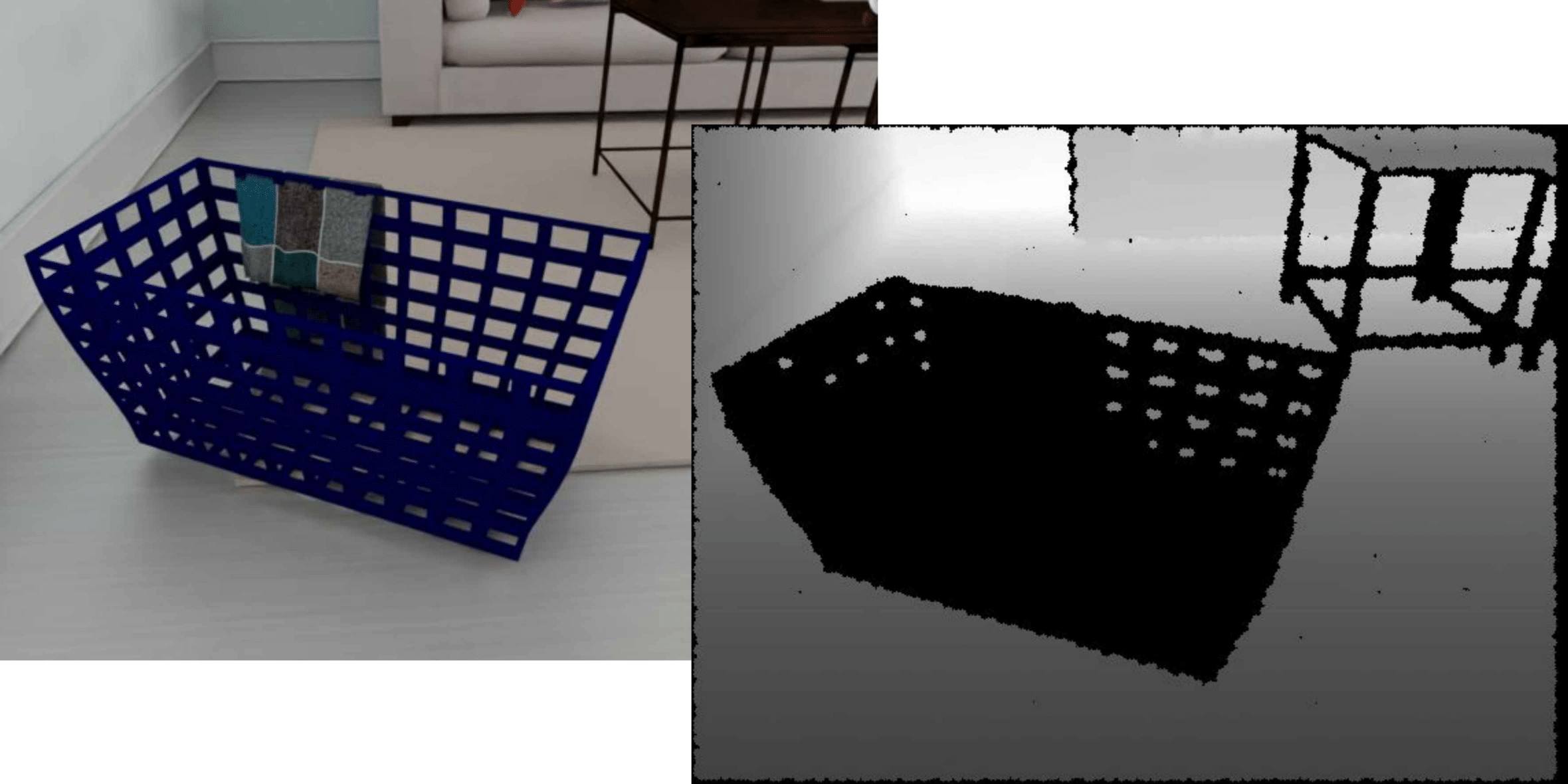
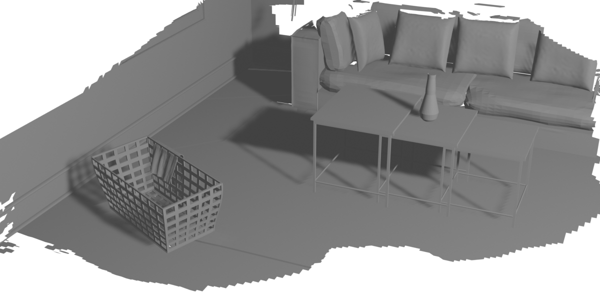
RGB-D Input	Ground Truth
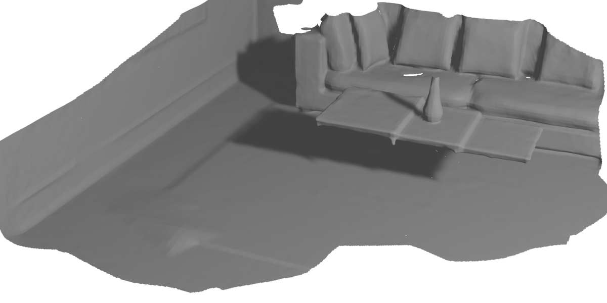
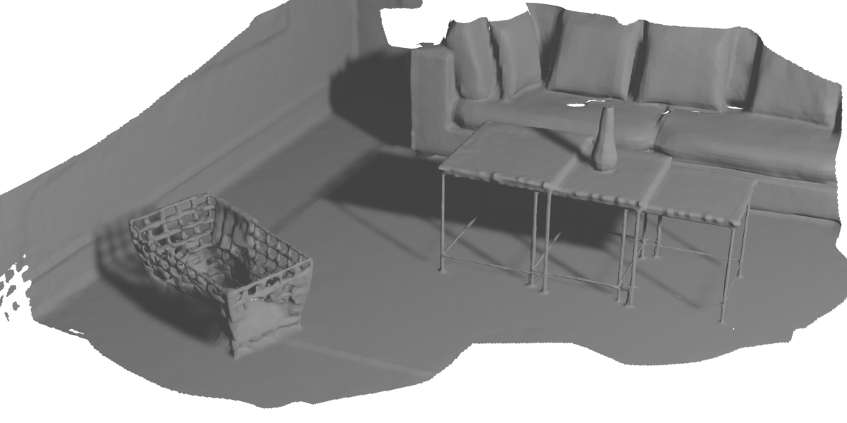
Ours w/o RGB term	Ours-full

Figure 2: Qualitative reconstruction results on synthetic sequence with thin geometries and missing depth measurements.

For the experiment on the synthetic scene, we simulate missing depth by removing the depth measurements from the baskets and table legs (top left corner in Fig. 2). Comparison in Fig. 2 demonstrates that RGB loss term is able to recover thin structures with missing depth and produce complete reconstruction. Tab. 3 also shows our full model achieves significantly better reconstruction quality, especially completeness.

Method	Acc.) $\downarrow$	Com. $\downarrow$	C-$\ell_{1}$ $\downarrow$	NC $\uparrow$	F-score $\uparrow$
Ours (no rgb)	0.0087	0.0291	0.0189	0.8967	0.9273
Ours (full)	0.0093	0.0121	0.0107	0.8986	0.9817

Table 3: We evaluate the reconstruction results of our model with out RGB loss term and our full model on a synthetic sequence with thin geometries.

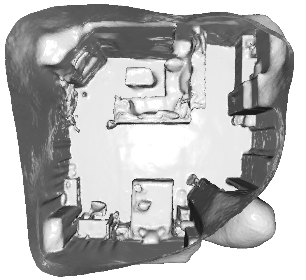
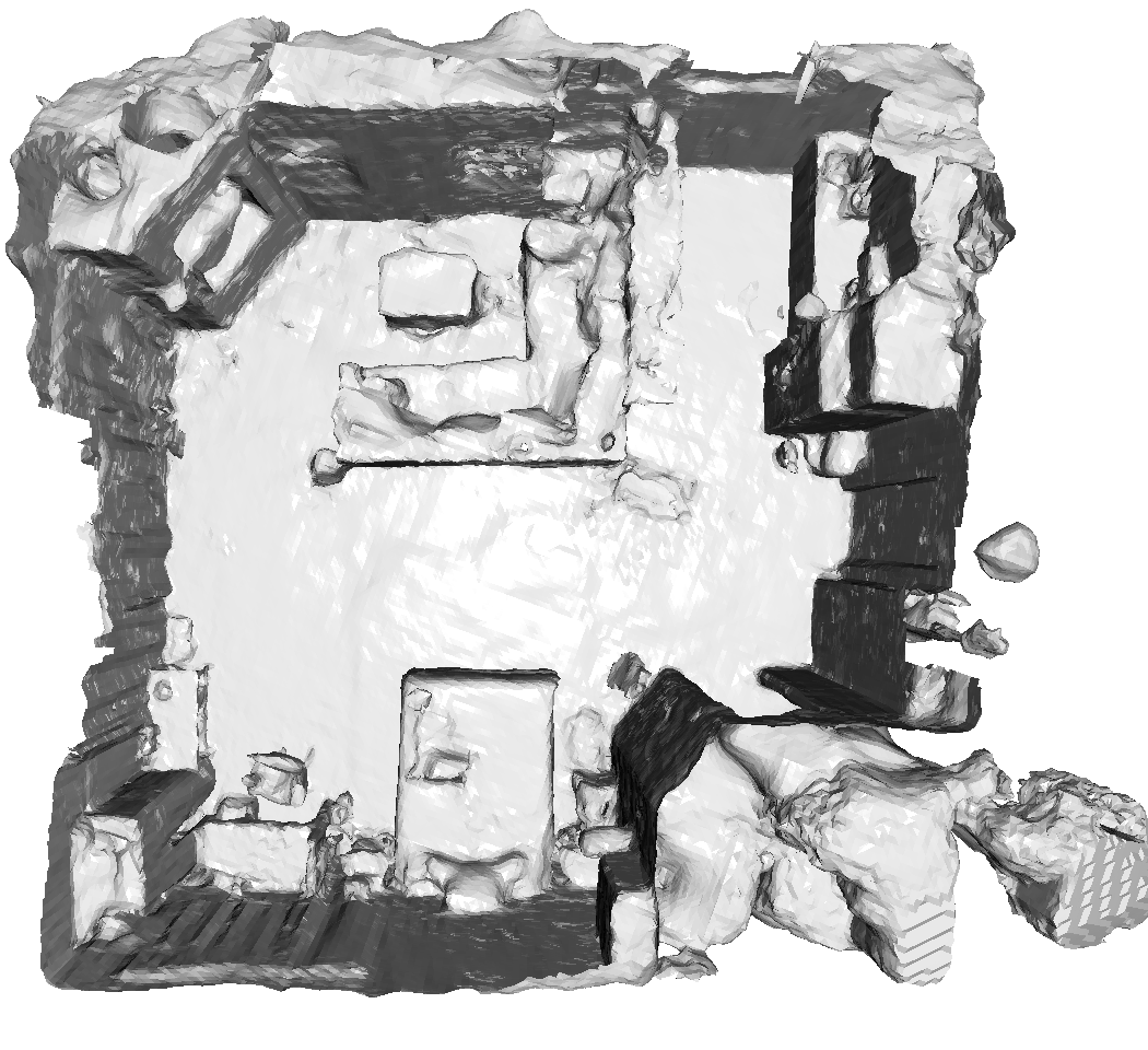
GO-Surf (Ours)	NICE-SLAM [6]

Figure 3: Reconstructed meshes (unculled) of sequential mapping on ScanNet scene0000. Note that for fair comparison NICE-SLAM is running in mapping mode with ground truth camera poses. GO-Surf runs over $\times 30$ faster while achieving much smoother high-quality reconstruction.

3.2 Effect of SDF Regularisation Terms

In this section we provide additional ablation studies on the two SDF regularisation terms.

Eikonal Term

The Eikonal term encourages the model prediction to be a valid signed distance field. We observe that without the Eikonal term the SDF values are being reconstructed only within the truncation region (i.e. very close to the surface). The Eikonal term helps correct SDF values to be propagated outside of the truncation region, although some local artefacts still remain (see Fig. 4) which we suspect are due to the local nature of gradients in the feature grid.

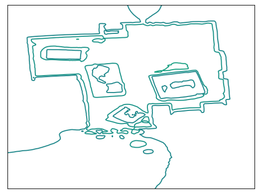
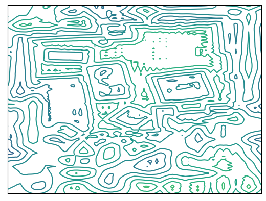
Full model	w/o Eikonal term	w/o Geometric initialisation

Figure 4: We found that applying the Eikonal term to some extent propagates the SDF gradient to empty spaces. Without the Eikonal term SDF is reconstructed only within the truncation region. Geometric initialisation reduces the noise in the unobserved regions (e.g. behind walls).

Normal Smoothness Term

We found that the normal smoothness term fills the holes in unobserved regions which is particularly useful for fixing discontinuities in large planar structures like walls or floor. It also encourages surface smoothness in all other areas, usually at the cost of some fine details. We investigate different settings of normal smoothness radius (see Fig. 5).

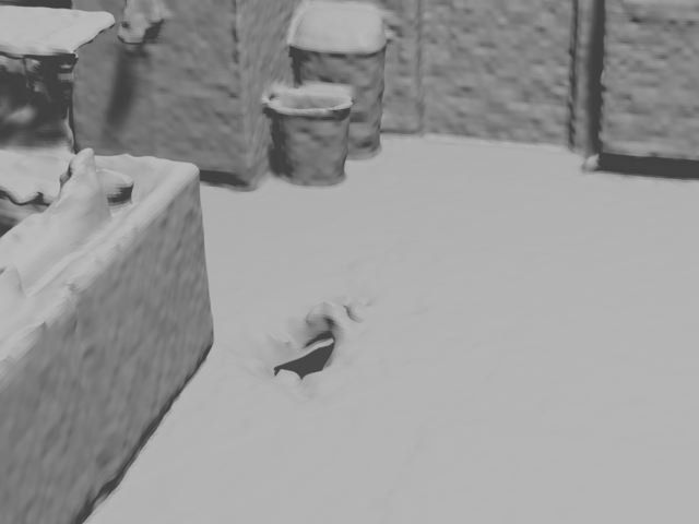
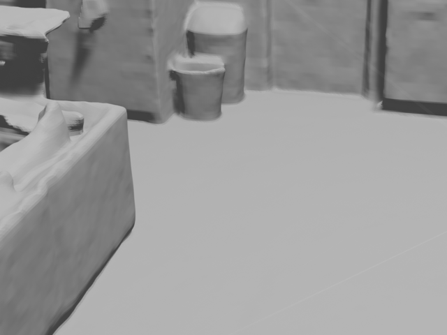
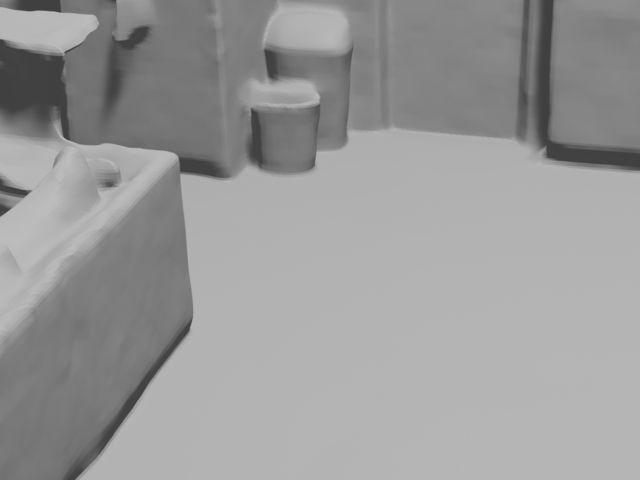
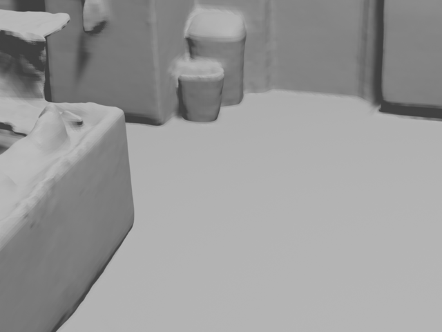
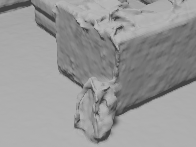
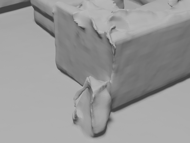
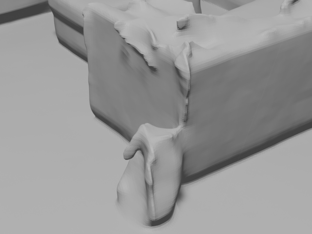
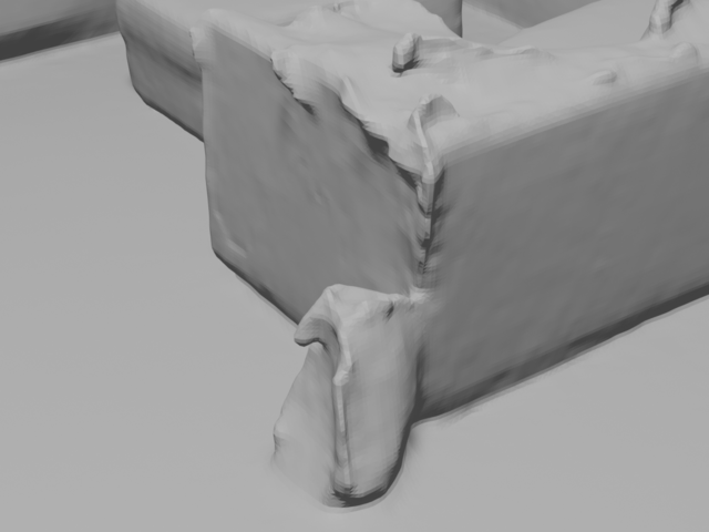
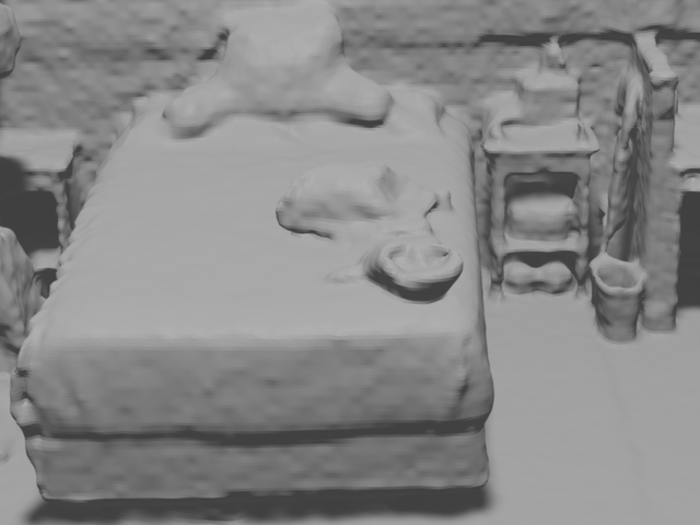
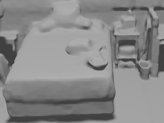
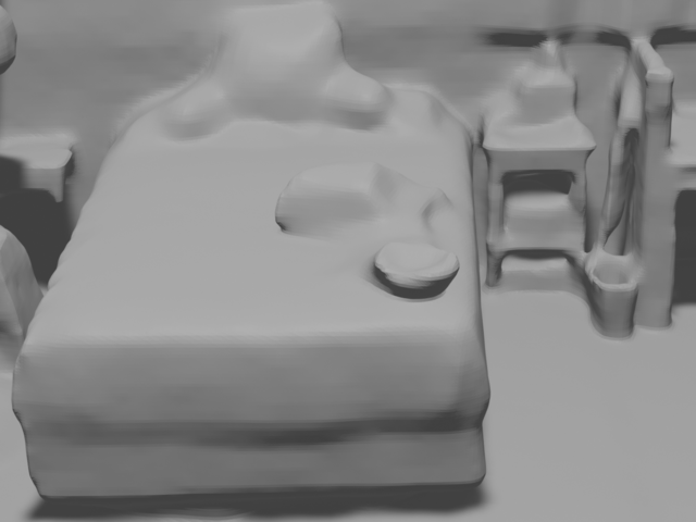
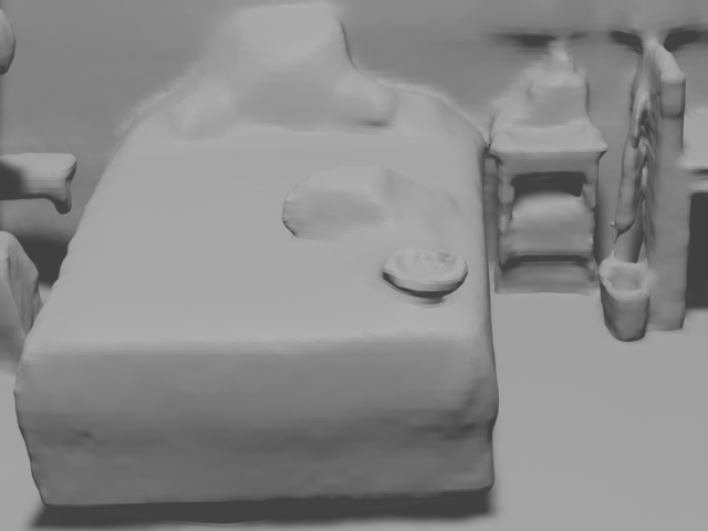
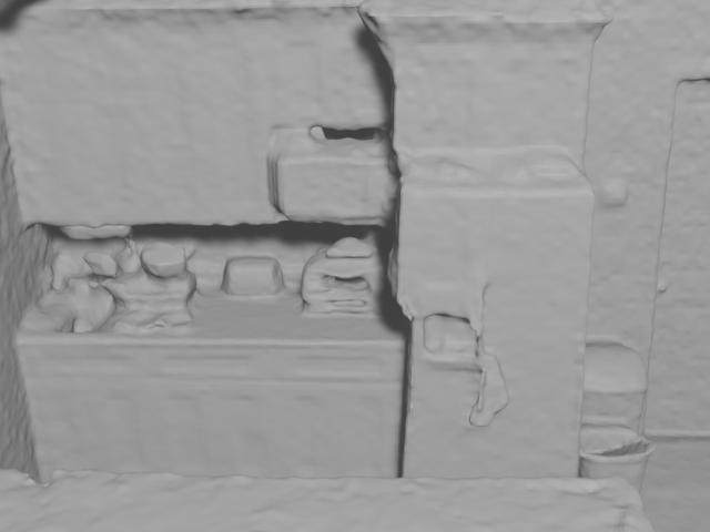
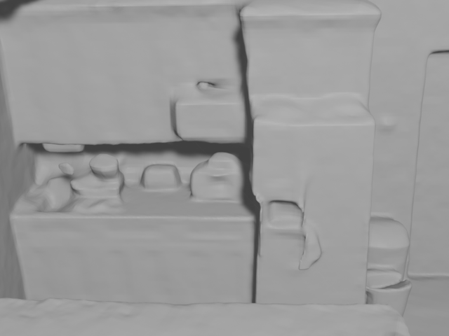
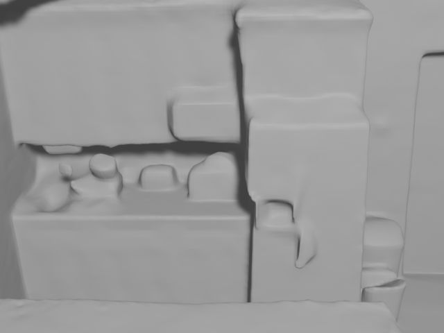
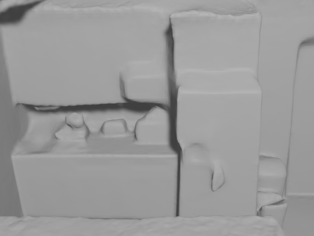
$\delta_{s}=0$ (no reg.)	$\delta_{s}=5\text{mm}$	$\delta_{s}=2\text{cm}$	$\delta_{s}=10\text{cm}$

Figure 5: Ablation study on effect of smoothness prior. We compare the reconstruction results with different values of $\delta_{s}$ for normal regularisation term. With $\delta_{s}=0$ the results capture more details like the backpack strap and tiny objects on the kitchen table, but also have more high frequency noises. Also the hole shows up near the sofa. Increasing $\delta_{s}$ to $10\text{cm}$ results in over-smoothed reconstruction. We empirically found $2-5\text{mm}$ is a good trade-off between smoothness and details.

4 More Results

In this section, we show more qualitative reconstruction results on synthetic scenes. Note that in order to also showcase the scene completion ability of different methods, the results shown here are from unculled meshes. Fig. 6 shows the comparison of our method to NeuralRGB-D and other learning-based methods. Overall, our method produces smoother, and more complete reconstruction without losing tiny details.

From the first two columns it can be seen that both NeuralRGB-D and our method have the ability to fill in unobserved regions (windows and the top ceiling). However, NeuralRGB-D tends to produce noisier scene completion results with many artefacts whereas ours is much smoother and looks more natural. In Fig 7 we provide more results to further showcase our method’s advantage over NeuralRGB-D in terms of scene completion.

BundleFusion [3]
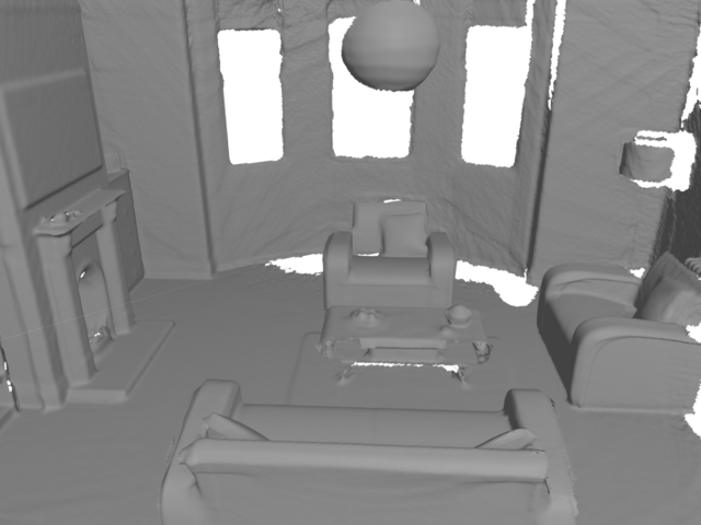
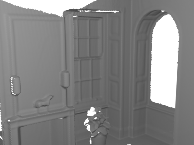
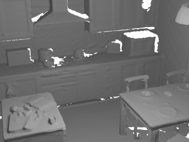
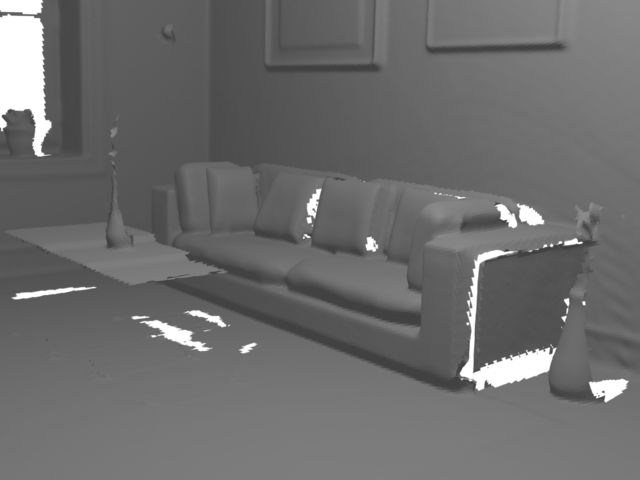
ConvOccNets [4]
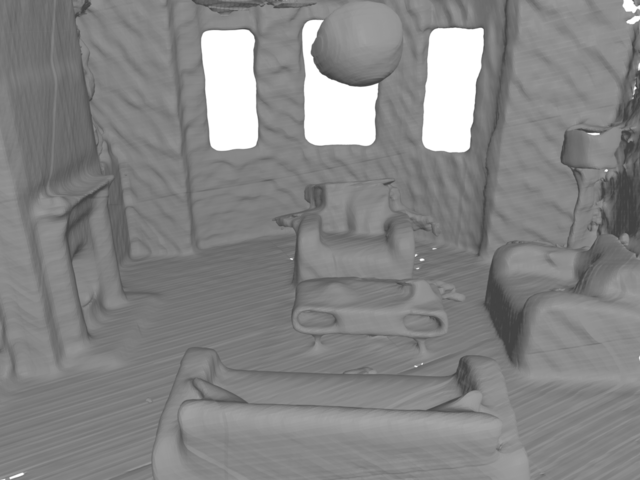
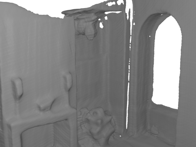
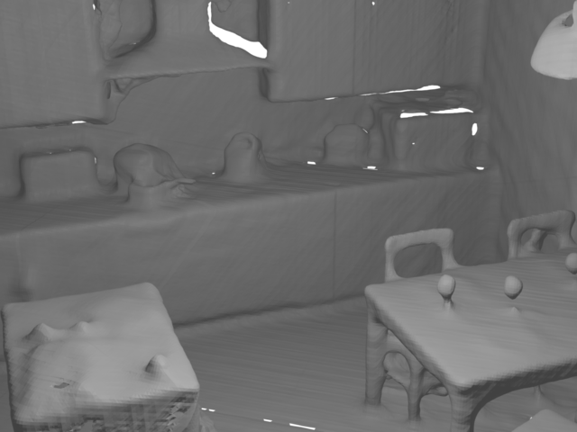
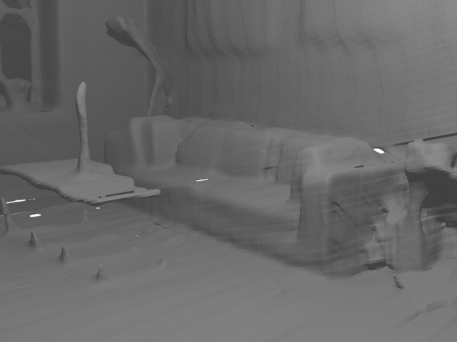
SIREN [5]
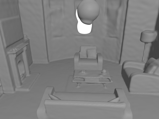
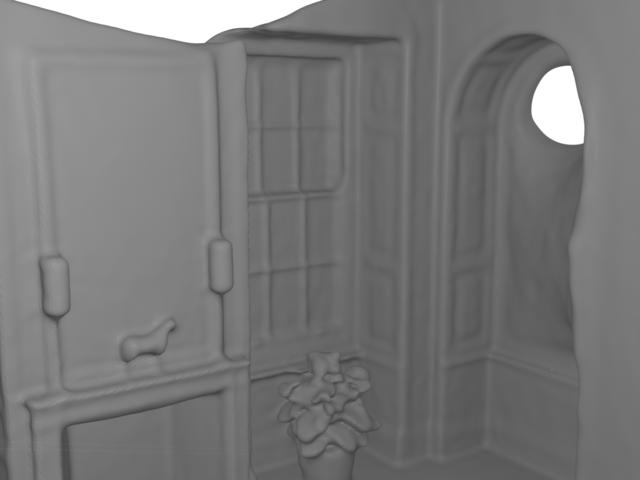
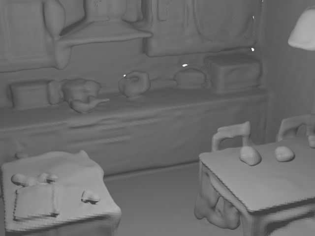
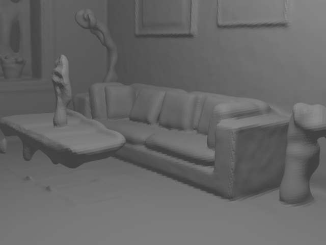
NeuralRGBD [1]
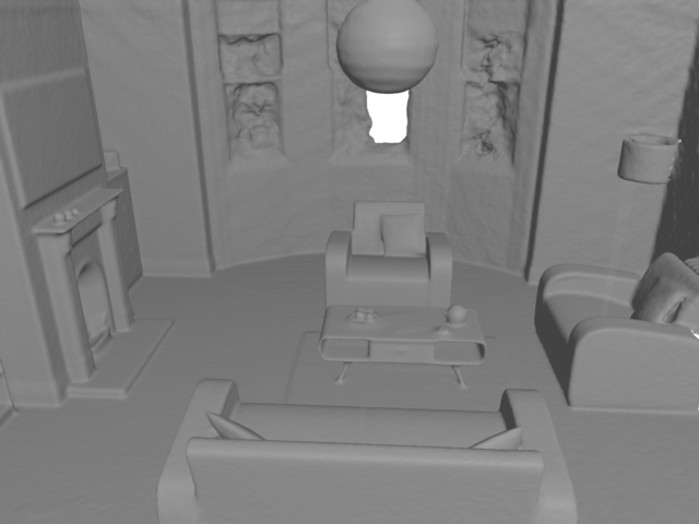
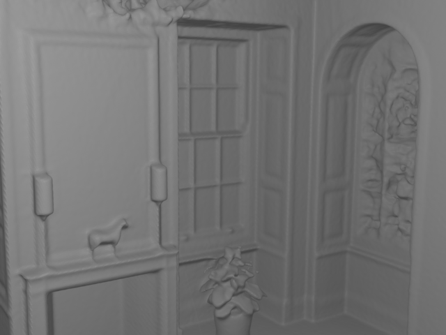
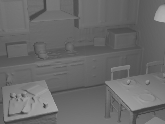
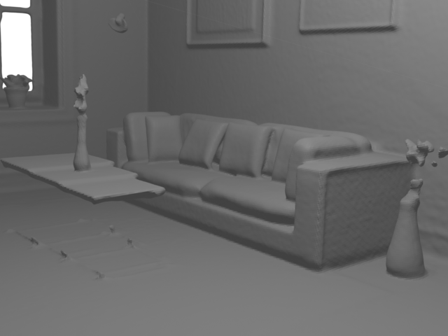
GO-Surf (Ours)
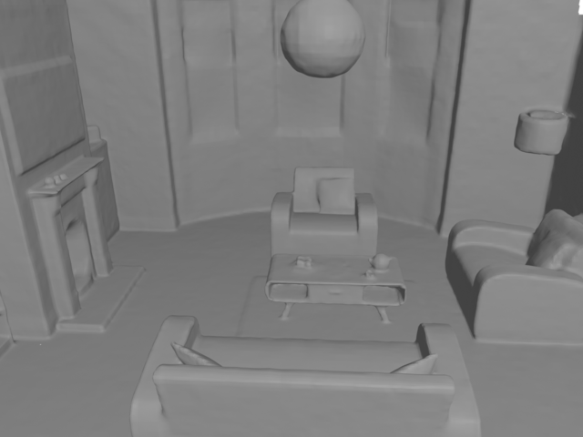
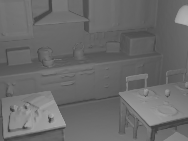
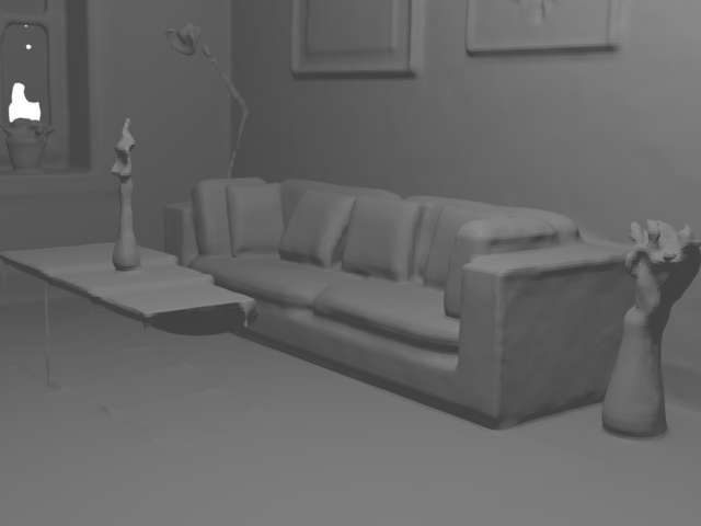
GT

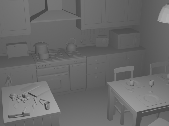
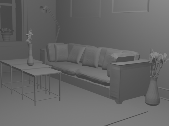
Figure 6: Qualitative comparison on synthetic scenes. GO-Surf produces smoother, and more complete reconstruction without losing tiny details. Both NeuralRGBD and our method have the scene completion ability. However, NeuralRGBD produces much noisier completion results with many artefacts whereas ours is much smoother and looks more natural.

BundleFusion [3]
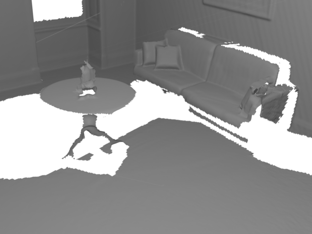
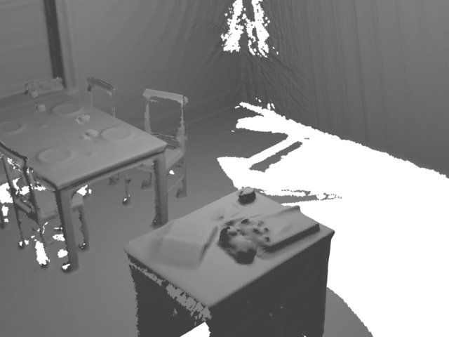
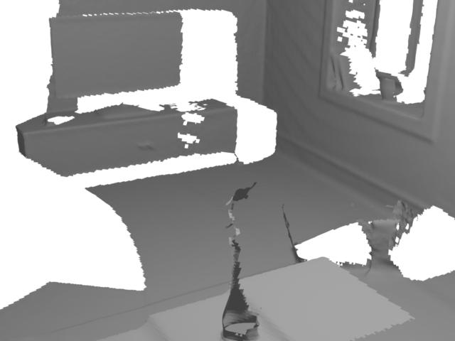
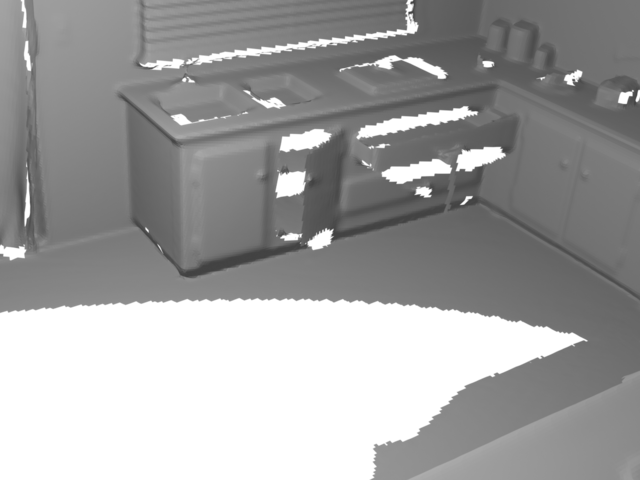
NeuralRGBD [1]
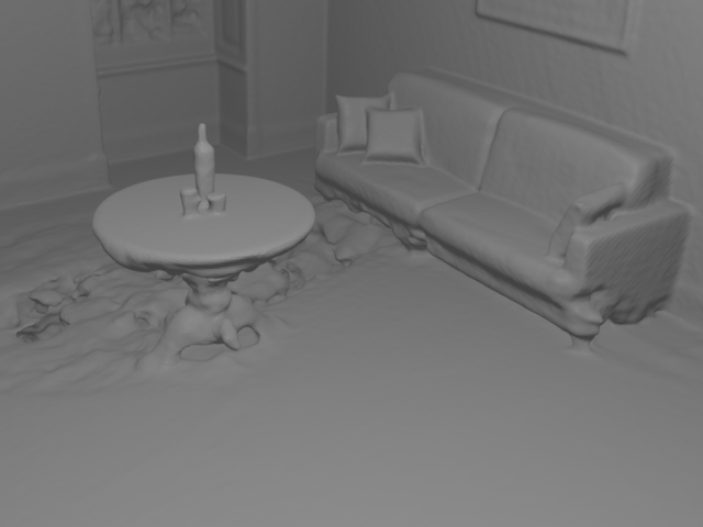
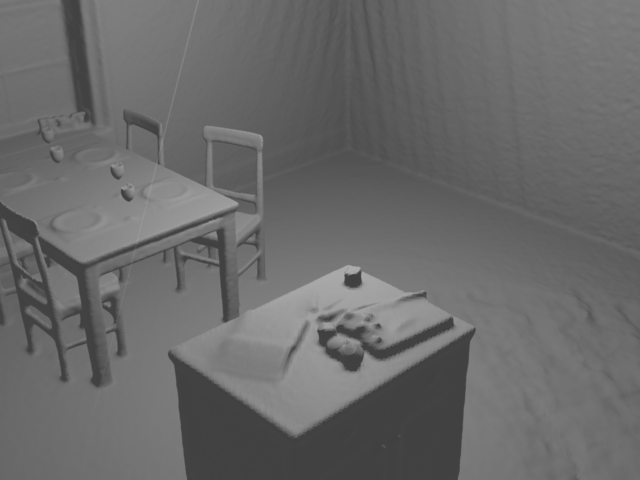
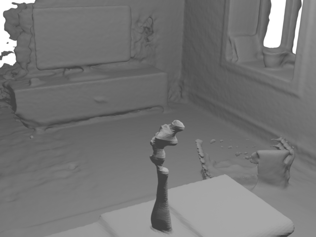
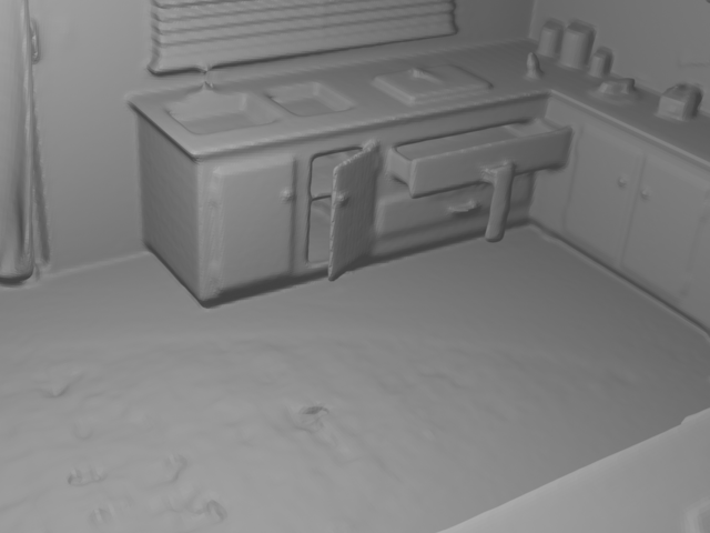
GO-Surf (Ours)
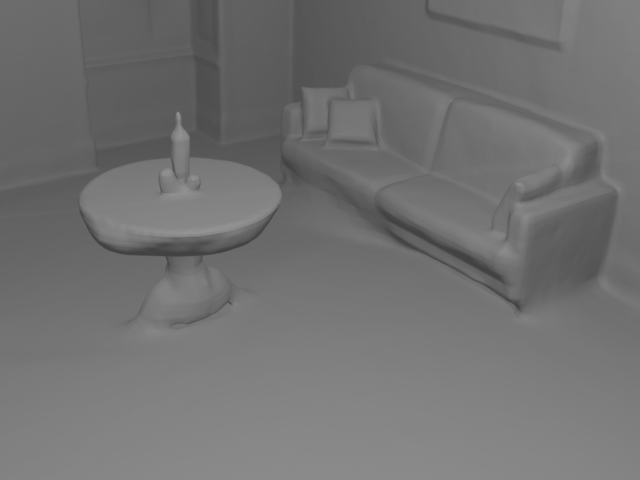
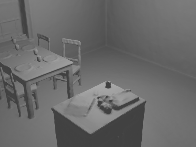
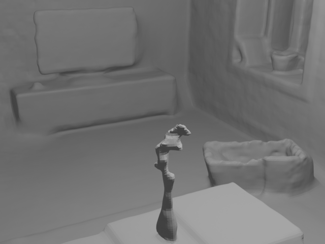
GT

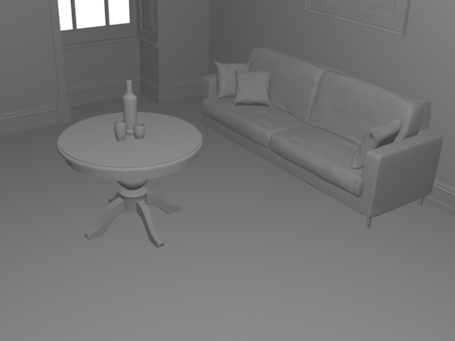
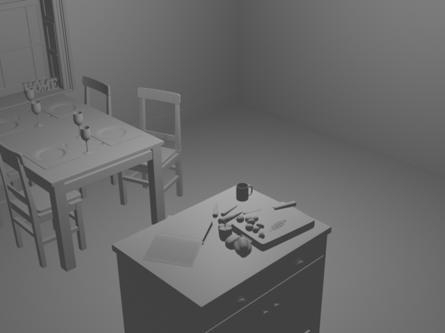
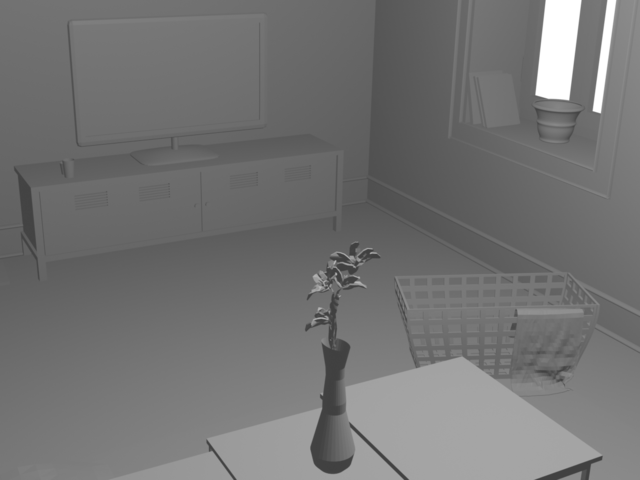
Figure 7: Scene completion comparison. NeuralRGBD produces much noisier completion results with many artefacts whereas ours is much smoother and looks more natural.

scene	scene dim.	voxel dim.	runtime	num params.	model size
complete kitchen	$9.3\times 10.0\times 3.3$	$321\times 353\times 129$	$45\text{ min}$	$73.1\text{ M}$	$294\text{ MB}$
kitchen	$7.0\times 8.7\times 3.4$	$257\times 321\times 129$	$40\text{ min}$	$53.2\text{ M}$	$214\text{ MB}$
breakfast room	$4.1\times 4.7\times 3.3$	$161\times 193\times 129$	$25\text{ min}$	$20.1\text{ M}$	$81\text{ MB}$
morning apartment	$3.5\times 4.0\times 2.3$	$129\times 161\times 97$	$19\text{ min}$	$10.1\text{ M}$	$41\text{ MB}$
grey white room	$5.9\times 4.4\times 3.1$	$225\times 161\times 129$	$24\text{ min}$	$23.4\text{ M}$	$94\text{ MB}$
white room	$5.6\times 7.9\times 3.8$	$193\times 289\times 161$	$39\text{ min}$	$44.9\text{ M}$	$181\text{ MB}$
staircase	$6.8\times 6.5\times 3.7$	$257\times 225\times 161$	$39\text{ min}$	$46.6\text{ M}$	$188\text{ MB}$
green room	$8.0\times 4.7\times 3.1$	$289\times 193\times 129$	$30\text{ min}$	$36.0\text{ M}$	$145\text{ MB}$
thin geometry	$3.4\times 3.6\times 1.2$	$129\times 129\times 65$	$15\text{ min}$	$5.4\text{ M}$	$28\text{ MB}$
ICL living room	$5.3\times 2.9\times 5.4$	$193\times 193\times 129$	$24\text{ min}$	$24.1\text{ M}$	$97\text{ MB}$
scene 0000	$8.8\times 9.1\times 3.4$	$321\times 321\times 129$	$44\text{ min}$	$66.5$ M	$268\text{ MB}$
scene 0002	$4.4\times 6.0\times 3.5$	$161\times 225\times 129$	$28\text{ min}$	$23.4$ M	$113\text{ MB}$
scene 0005	$5.8\times 5.3\times 2.9$	$225\times 193\times 125$	$33\text{ min}$	$27.1$ M	$113\text{ MB}$
scene 0012	$5.8\times 5.7\times 2.9$	$225\times 225\times 129$	$31\text{ min}$	$32.7$ M	$132\text{ MB}$
scene 0024	$7.6\times 8.4\times 2.9$	$289\times 289\times 129$	$40\text{ min}$	$53.9$ M	$217\text{ MB}$
scene 0050	$5.9\times 4.5\times 3.1$	$225\times 161\times 129$	$26\text{ min}$	$23.4$ M	$94\text{ MB}$

Table 4: Runtime and memory requirement on synthetic and ScanNet [2] scenes. We list scene dimension ($\text{m}^{3}$), voxel dimension, runtime (min), number of model parameters and model size (MB). Our method requires much less runtime than NeuralRGBD [1] ($15-45\text{ min}$ vs $15-25\text{ hours}$) at the cost of larger model size (tens to hundreds of MB vs several MB).

5 Runtime and Memory Analysis

In Tab. 4 we provide detailed breakdown of of the runtime and memory usage of our method on all of the scenes that we had run experiments on. Our method requires $15$ to $45$ minutes to converge which is approximately $\times 60$ faster than NeuralRGB-D. However our model size is much larger (tens to hundreds million of parameters vs several million parameters) and scales rapidly as the scene gets larger. This is This is an inherent problem of voxel-like architectures as the number of voxels scales cubically with the scene dimension. Voxel hashing or octree-based sparsification could be adopted to significantly reduce the memory footprint of our system and we intend to explore this direction in future work.

6 Sequential Mapping Experiments

GO-Surf’s fast runtime also enables sequential/online mapping at interactive framerate with slightly reduced resolution. In this section we run GO-Surf in a sequential fashion using $3$-level feature grid with voxel sizes of $6\text{cm}$, $24\text{cm}$ and $96\text{cm}$ on ScanNet scene0000 and compare against NICE-SLAM [6] running on the same scene with ground truth camera poses.

With increased voxel size GO-Surf runs in near real-time at $15\text{Hz}$ while NICE-SLAM runs much slower below $0.5\text{Hz}$. Fig 3 shows the comparison of reconstruction results. Ours is much smoother and has has less artifacts.

References

- [1] Dejan Azinović, Ricardo Martin-Brualla, Dan B Goldman, Matthias Nießner, and Justus Thies. Neural rgb-d surface reconstruction. In Proceedings of the IEEE/CVF Conference on Computer Vision and Pattern Recognition (CVPR), June 2022.
- [2] Angela Dai, Angel X. Chang, Manolis Savva, Maciej Halber, Thomas Funkhouser, and Matthias Nießner. Scannet: Richly-annotated 3d reconstructions of indoor scenes. In Proc. Computer Vision and Pattern Recognition (CVPR), IEEE, 2017.
- [3] Angela Dai, Matthias Nießner, Michael Zollhöfer, Shahram Izadi, and Christian Theobalt. Bundlefusion: Real-time globally consistent 3d reconstruction using on-the-fly surface reintegration. ACM Transactions on Graphics (TOG), 36(4):76a, 2017.
- [4] Songyou Peng, Michael Niemeyer, Lars Mescheder, Marc Pollefeys, and Andreas Geiger. Convolutional occupancy networks. In European Conference on Computer Vision (ECCV), Cham, Aug. 2020. Springer International Publishing.
- [5] Vincent Sitzmann, Julien N.P. Martel, Alexander W. Bergman, David B. Lindell, and Gordon Wetzstein. Implicit neural representations with periodic activation functions. In arXiv, 2020.
- [6] Zihan Zhu, Songyou Peng, Viktor Larsson, Weiwei Xu, Hujun Bao, Zhaopeng Cui, Martin R. Oswald, and Marc Pollefeys. Nice-slam: Neural implicit scalable encoding for slam. In Proceedings of the IEEE/CVF Conference on Computer Vision and Pattern Recognition (CVPR), 2022.