Abstract

When observations are truncated, we are limited to an incomplete picture of our dataset. Recent methods deal with truncated density estimation problems by turning to score matching, where the access to the intractable normalising constant is not required. We present a novel extension to truncated score matching for a Riemannian manifold. Applications are presented for the von Mises-Fisher and Kent distributions on a two dimensional sphere in $\mathbb{R}^{3}$, as well as a real-world application of extreme storm observations in the USA. In simulated data experiments, our score matching estimator is able to approximate the true parameter values with a low estimation error and shows improvements over a maximum likelihood estimator.

1 Introduction

Often, data can only be observed within a certain ‘window’ of observations, such as a physical threshold (e.g., the borders of a country). This could include applications such as weather events, under-reported count data in disease modelling or undiscovered locations of wildlife habitats. Conventional statistical estimation methods are designed for datasets with full observations, even if this is not always the case. To address this complicated problem, it becomes necessary to extend existing methodology to account for this truncation of data when performing parameter estimation.

In this paper, we consider truncated densities on manifolds. Truncated density estimation on a manifold has a vast potential for applications such as in earth science applications. Estimation in a truncated setting on Earth with a Euclidean approximation may yield inaccurate results if the region is large enough due to its curvature. Additionally, artificial boundaries exist in the case of continental or national borders, which naturally span a large area of the world. When collecting observations of environmental variables, countries may only measure events that happen within their border, but not the phenomena which occur outside of their borders, for example in neighbouring countries or the ocean.

One issue with estimating a truncated density is the evaluation of the normalising constant of a statistical model, which is often intractable in such a scenario. Estimation of unnormalised models are encountered in applications such as Markov random fields for image analysis (Li, 2009), non-Gaussian undirected graphical models, and independent component analysis (Teh et al., 2003). Score matching is a statistical estimation method which bypasses the evaluation of this normalising constant, making it suitable for estimating truncated densities. Score matching has seen many developments in recent years (Hyvärinen, 2005; 2007). Recent work has proposed a generic score matching objective to estimate a truncated density function Yu et al. (2021); Liu et al. (2022). Methodology also exists for estimating a non-truncated statistical model on a manifold (Mardia et al., 2016). However, no known score matching variant currently exists which estimates a truncated density on a manifold. In this work, we proposes an efficient estimator that estimates such a truncated statistical model without requiring a normalising constant.

2 Background

2.1 Score Matching

Firstly, let us define a parametric statistical model as

$$p(\boldsymbol{x};\boldsymbol{\beta})=\frac{1}{Z(\boldsymbol{\beta})}\bar{p}(\boldsymbol{x};\boldsymbol{\beta}),\qquad Z(\boldsymbol{\beta})=\int_{V}\bar{p}(\boldsymbol{x};\boldsymbol{\beta})d\boldsymbol{x},$$

for some domain $V$ (e.g. $V=\mathbb{R}^{d}$), and where $p(\boldsymbol{x};\boldsymbol{\beta})$ is the probability density function (pdf). We use this model to approximate an unknown data density function $q(\boldsymbol{x})$, where $\boldsymbol{\beta}$ is the parameter which would like to estimate. In many cases, the normalising constant, $Z(\boldsymbol{\beta})$, is intractable, therefore classical methods such as maximum likelihood estimation (MLE) are unsuited. Instead, one often turns to methods such as score matching (Hyvärinen, 2005; 2007), which minimises

$$J(\boldsymbol{\beta})=\int_{V}q(\boldsymbol{x})\left\lVert\boldsymbol{\psi}_{q}-\boldsymbol{\psi}_{p}\right\rVert_{2}^{2}d\boldsymbol{x},$$ (1)

since the score functions $\boldsymbol{\psi}_{q}=\boldsymbol{\nabla}_{\boldsymbol{x}}\log q(\boldsymbol{x})$ and $\boldsymbol{\psi}_{p}=\boldsymbol{\nabla}_{\boldsymbol{x}}\log p(\boldsymbol{x};\boldsymbol{\beta})$ do not depend on the normalising constant. The later inclusion of a ‘scaling function’ $g(\boldsymbol{x})>0$ yields the generalised score matching estimator (Lin et al., 2016; Yu et al., 2016; 2019):

$$J(\boldsymbol{\beta})=\int_{V}q(\boldsymbol{x})g(\boldsymbol{x})\left\lVert\boldsymbol{\psi}_{q}-\boldsymbol{\psi}_{p}\right\rVert_{2}^{2}d\boldsymbol{x}.$$ (2)

Under some mild regularity conditions, the objective function in (2) can be written as

$$\begin{split}J(\boldsymbol{\beta})=\int_{V}q(\boldsymbol{x})\Big{(}&g(\boldsymbol{x})\Big{[}\boldsymbol{\psi}_{p}^{2}+2\mathrm{tr}\left\{\boldsymbol{\nabla}_{\boldsymbol{x}}\boldsymbol{\psi}_{p}\right\}\Big{]}\\ &+2\left\langle\boldsymbol{\nabla}_{\boldsymbol{x}}g(\boldsymbol{x}),\boldsymbol{\psi}_{p}\right\rangle\Big{)}d\boldsymbol{x}+\text{const},\end{split}$$ (3)

where $\nabla_{\boldsymbol{x}}\boldsymbol{\psi}_{p}$ denotes the hessian of $\log p(\boldsymbol{x};\beta)$. This formulation is derived using integration by parts (see Theorem 3, Yu et al. (2019)). Now the objective no longer depends on the density of the unknown data $q(\boldsymbol{x})$, and thus the estimator of $\boldsymbol{\beta}$ is given by $\boldsymbol{\hat{\beta}}\vcentcolon=\operatorname*{arg\,min}_{\boldsymbol{\beta}}\tilde{J}(\boldsymbol{\beta})$.

In a truncated setting, consider a bounded open subspace $V\subset\mathbb{R}^{d}$, where the boundary of the subspace is denoted by $\partial V$. We observe only $\boldsymbol{x}\in V$, thus the normalization constant $Z(\beta)$ is intractable, therefore score matching is a natural choice of method for estimation. However, the conditions which allowed the score matching objective (2) to be written tractably as (3) are no longer valid when truncated. Instead, Liu et al. (2022) introduced an extension which enforced $g(\boldsymbol{x}^{\prime})=0$ for all $\boldsymbol{x}^{\prime}\in\partial V$. By including this constraint on $g$, the integration by parts required for a tractable score matching objective now holds for the truncated case.

Liu et al. (2022) proposed the use of a specific family of $g$ functions given by distance metrics. For example, the Euclidean distance given by $g(\boldsymbol{x})=\min_{\boldsymbol{\tilde{x}}\in\partial V}\left\lVert\boldsymbol{x}-\boldsymbol{\tilde{x}}\right\rVert_{2}$. Distance functions naturally satisfy the criteria for $g(\boldsymbol{x})$.

Separately, Mardia et al. (2016) proposed a variant of score matching that is defined on a compact oriented Riemannian manifold $M$. Mardia et al. modified the classical score matching objective function given in (1) to include integration over the manifold:

$$J_{M}(\boldsymbol{\beta})\vcentcolon=\frac{1}{2}\int_{M}q(\boldsymbol{x})\left\lVert\boldsymbol{\psi}_{q}-\boldsymbol{\psi}_{p}\right\rVert_{2}^{2}d\boldsymbol{x}.$$ (4)

They made use of the the following integration by parts as a consequence of Stokes’ Theorem (Stewart et al., 2020):

Theorem 2.1.

Let $f_{1}$ and $f_{2}$ be continuous twice differentiable functions on a compact Riemannian manifold $M$, then

$$\begin{split}\oint_{\partial M}f_{1}(\boldsymbol{x})&\frac{\partial\boldsymbol{\nabla}_{\boldsymbol{x}}f_{2}(\boldsymbol{x})}{\partial\mathbf{n}}\partial M=\int_{M}(\boldsymbol{\Delta}_{M}f_{2}(\boldsymbol{x}))f_{1}(\boldsymbol{x})d\boldsymbol{x}\\ &+\int_{M}\langle\boldsymbol{\nabla}_{\boldsymbol{x}}f_{1}(\boldsymbol{x}),\boldsymbol{\nabla}_{\boldsymbol{x}}f_{2}(\boldsymbol{x})\rangle_{M}d\boldsymbol{x}.\end{split}$$ (5)

where $\mathbf{n}$ is the unit normal vector.

Additionally, let us define the Laplace-Beltrami operator, which is given by

$$\boldsymbol{\Delta}_{M}u=\mathrm{tr}\left\{\mathbf{P}\boldsymbol{\nabla}_{\boldsymbol{x}}\cdot\left(\mathbf{P}\boldsymbol{\nabla}_{\boldsymbol{x}}\tilde{u}\right)\right\},$$ (6)

and the manifold inner product, which is defined as

$$\langle u,v\rangle=\langle\mathbf{P}\tilde{u},\mathbf{P}\tilde{v}\rangle$$ (7)

where $u$ is a continuous twice differentiable real-valued function on $M$, $\tilde{u}$ is the extension of $u$ to a neighbourhood $N\subset\mathbb{R}^{m}$ of $M$, and $\mathbf{P}$ is the $m\times m$ orthogonal projection matrix onto the $m$-dimensional tangent hyperplane to $M$.

Mardia et al. (2016) used Theorem 2.1 to rewrite (4) (up to a constant) as

$$\begin{split}J_{M}(\boldsymbol{\beta})=\int_{M}q(\boldsymbol{x})\big{[}\langle&\boldsymbol{\psi}_{p},\boldsymbol{\psi}_{p}\rangle_{M}\\ &+2(\boldsymbol{\Delta}_{M}\log p(\boldsymbol{x};\boldsymbol{\beta}))\big{]}d\boldsymbol{x},\end{split}$$ (8)

which, as an expectation, no longer involves the unknown data density $q(\boldsymbol{x})$, see Section 3, Mardia et al. (2016) for details. This step is an analogue to using integration-by-parts in classical score matching to derive a tractable objective function.

Expectations in the objective functions in both (3) and (8) can be replaced with their Monte Carlo approximations to yield a tractable equation.

2.2 Distributions on Spheres

We consider two primary probability distributions on the unit hypersphere ($S^{d-1}$) in $\mathbb{R}^{d}$: the Kent distribution (or Fisher-Bingham distribution) and the von-Mises Fisher distribution. See Chapter 9, Mardia & Jupp (2009) for an overview of spherical distributions.

2.2.1 Kent Distribution

The pdf for the Kent distribution is

$$p(\boldsymbol{x};\boldsymbol{\beta})=\frac{1}{Z(\kappa,\boldsymbol{\alpha})}\exp\{\kappa\boldsymbol{\mu}^{\top}\boldsymbol{x}+\sum_{j=1}^{d-1}\alpha_{j}(\boldsymbol{\gamma}_{j}^{\top}\boldsymbol{x})^{2}\},$$

for $\boldsymbol{x}\in\mathbb{R}^{d}$, where $Z(\kappa,\boldsymbol{\alpha})$ is the normalising constant (Kent, 1982). Here, $\boldsymbol{\mu}$ is the mean direction, whilst the $\boldsymbol{\gamma}_{j}$ are the axes which determine the orientation of the probability contours. The $\kappa$ parameter is the concentration parameter, and the $\alpha_{j}$ are the ovalness parameters, which determines how elliptical the distribution is (Mardia & Jupp, 2009).

For $S^{2}$ in $R^{3}$, the first and second derivatives of the log pdf can be calculated as

$$\boldsymbol{\psi}_{p} =\kappa\boldsymbol{\mu}+2\alpha\left[\boldsymbol{\gamma}_{1}(\boldsymbol{\gamma}_{1}^{\top}\boldsymbol{x})-\boldsymbol{\gamma}_{2}(\boldsymbol{\gamma}_{2}^{\top}\boldsymbol{x})\right],$$ (9)

$$\boldsymbol{\nabla}_{\boldsymbol{x}}\boldsymbol{\psi}_{p} =2\alpha\left[\boldsymbol{\gamma}_{1}^{\top}\boldsymbol{\gamma}_{1}-\boldsymbol{\gamma}_{2}^{\top}\boldsymbol{\gamma}_{2}\right].$$ (10)

The Kent distribution is analogous to the Multivariate Normal (MVN) distribution on $\mathbb{R}^{d}$, and has similar properties, such as $\kappa$, $\alpha_{j}$, and $\boldsymbol{\gamma}_{j}$ controlling the shape of the data distribution, similar to the role of the covariance matrix of the MVN.

2.2.2 von Mises-Fisher Distribution

The von Mises-Fisher distribution is a special case of the Kent distribution where $\alpha=0$. It has pdf

$$p(\boldsymbol{x};\boldsymbol{\beta})=\frac{1}{Z(\kappa)}\exp\{\kappa\boldsymbol{\mu}^{\top}\boldsymbol{x}\},$$

for $\boldsymbol{x}\in\mathbb{R}^{d}$. Here, $Z(\kappa)$ is the normalising constant, $\boldsymbol{\mu}$ is the mean direction and $\kappa$ is the concentration parameter (Mardia & Jupp, 2009); all defined as in the Kent distribution. The gradients of the log probability density function are calculated as

$$\boldsymbol{\psi}_{p} =\kappa\boldsymbol{\mu},$$ (11)

$$\boldsymbol{\nabla}_{\boldsymbol{x}}\boldsymbol{\psi}_{p} =\mathbf{0}_{d\times d},$$ (12)

where $\mathbf{0}_{d\times d}$ denotes the $d\times d$ matrix of zeros. The von Mises-Fisher distribution can also be considered as analogous to the MVN with mean $\boldsymbol{\mu}$ and covariance matrix $\boldsymbol{\Sigma}=\kappa^{-1}\mathbf{I}_{d}$.

3 Truncated Manifold Score Matching

We extend the approach of both Liu et al. (2022) and Mardia et al. (2016) to combine truncated and manifold score matching. Consider a compact oriented Riemannian manifold $M$ with boundary $\partial M$, and random vector $\boldsymbol{x}\in M$ with pdf $q(\boldsymbol{x})$. Similar to previous score matching implementations by Hyvärinen (2005; 2007), Mardia et al. (2016) and Liu et al. (2022), we minimise the expected squared distance between the score functions of the statistical model and the data,

$$\begin{split}J_{S}(\boldsymbol{\beta}):=\frac{1}{2}\int_{M}q(\boldsymbol{x})g(\boldsymbol{x})\left\lVert\boldsymbol{\psi}_{q}-\boldsymbol{\psi}_{p}\right\rVert_{2}^{2}d\boldsymbol{x},\end{split}$$ (13)

where the integration is with respect to the manifold surface $M$, and $g(\boldsymbol{x})$ is the scaling function. In the classical score matching derivation, one part of the proof involves a term which is equal to zero under the assumption that the density $q(\boldsymbol{x})\to 0$ as $\boldsymbol{x}\to\infty$. In the truncated setting, this assumption is no longer valid, as the support of $q(\boldsymbol{x})$ ends at the boundary, $\partial M$, for which $q(\boldsymbol{x})\neq 0$. Instead, akin to the approach of Liu et al. (2022), we instead let $g(\boldsymbol{x}^{\prime})=0$ for all $\boldsymbol{x}^{\prime}\in\partial M$, the boundary of the manifold. This condition is necessary for the derivation of the following theorem.

Theorem 3.1.

(13) can be expressed as

$$\begin{split}J_{S}(\boldsymbol{\beta})=\int_{M}&q(\boldsymbol{x})g(\boldsymbol{x})\langle\boldsymbol{\psi}_{p},\boldsymbol{\psi}_{p}\rangle_{M}d\boldsymbol{x}\\ +&2\int_{M}q(\boldsymbol{x})g(\boldsymbol{x})\boldsymbol{\Delta}_{M}\log p(\boldsymbol{x};\boldsymbol{\beta})d\boldsymbol{x}\\ +&2\int_{M}q(\boldsymbol{x})\langle\boldsymbol{\nabla}_{\boldsymbol{x}}g(\boldsymbol{x}),\boldsymbol{\psi}_{p}\rangle_{M}d\boldsymbol{x},\end{split}$$ (14)

where the integration is over $M$, $\langle\cdot,\cdot\rangle_{M}$ is the manifold inner product and $\boldsymbol{\Delta}_{M}$ is the Laplace-Beltrami operator.

For proof, see Appendix A. Although we have not specified $g(\boldsymbol{x})$, we only need find a $g$ such that the condition for which $g(\boldsymbol{x}^{\prime})=0$ for all $x^{\prime}\in\partial M$ holds. Any such differentiable and strictly positive function which satisfies this boundary constraint is a valid choice of $g$. See Liu et al. (2022) for a comprehensive study of the choice of $g$ in a Euclidean setting. In section 3.2, we propose two distance functions that naturally fulfill this criteria, and are suited for the sphere.

The integrals can be approximated using samples from distribution $q(\boldsymbol{x})$ as

$$\begin{split}\tilde{J}_{S}(\boldsymbol{\beta})=&\frac{1}{n}\sum_{i=1}^{n}g(\boldsymbol{x}_{i})\langle\boldsymbol{\psi}_{p}^{(i)},\boldsymbol{\psi}_{p}^{(i)}\rangle_{M}\\ +&\frac{2}{n}\sum_{i=1}^{n}g(\boldsymbol{x}_{i})\mathrm{tr}\{\boldsymbol{\Delta}_{M}\log p(\boldsymbol{x}_{i};\boldsymbol{\beta})\}\\ +&\frac{2}{n}\sum_{i=1}^{n}\langle\boldsymbol{\nabla}_{\boldsymbol{x}}g(\boldsymbol{x}_{i}),\boldsymbol{\psi}_{p}^{(i)}\rangle_{M},\end{split}$$ (15)

provided that $n$ is sufficiently large, and where $\boldsymbol{\psi}_{p}^{(i)}=\boldsymbol{\nabla}_{\boldsymbol{x}}\log p(\boldsymbol{x}_{i};\boldsymbol{\beta})$ denotes the score function evaluated at the $i$-th data point. The score matching estimator is given by $\boldsymbol{\hat{\beta}}:=\operatorname*{arg\,min}_{\boldsymbol{\beta}}\tilde{J}_{S}(\boldsymbol{\beta}),$ which can be optimised numerically using gradient based methods.

3.1 Score Matching on Spherical Distributions

Section 2.2 describes two probability distributions defined on a unit sphere; the von Mises-Fisher distribution and the Kent distribution. The generalised manifold score matching approach detailed above is applicable to any manifold on which Stokes’ theorem (2.1) holds, which includes the unit $(d-1)$-hypersphere in $\mathbb{R}^{d}$ where the probability distributions on a sphere are well defined.

Spherical distributions can be defined in Euclidean coordinates, denoted $\boldsymbol{x}\in\mathbb{R}^{d}$, or as spherical coordinates, denoted $\boldsymbol{z}\in S^{d-1}$. Whilst the methods present in this research are applicable to high dimensional manifolds (and spheres), the two dimensional sphere is primarily considered as the application is clear.

On the 2D sphere, Euclidean coordinates have components $\boldsymbol{x}=(x_{1},x_{2},x_{3})\in\mathbb{R}^{3}$, whereas spherical coordinates have components $\boldsymbol{z}=(\theta,\phi)\in S^{2}$, where $\theta\in[0,\pi)$ is the colatitude and $\phi\in[0,2\pi]$ is the longitude. Conversion between spherical and Euclidean coordinates is given by

$$\boldsymbol{x}=(r\cos\phi,r\sin\phi\cos\theta,r\sin\phi\sin\theta),$$

and conversion from Euclidean coordinates to spherical coordinates is given by

$$\boldsymbol{z}=(\arccos\left(x_{1}/r\right),\arctan(x_{3}/x_{2})),$$ (16)

where $r=(x_{1}^{2}+x_{2}^{2}+x_{3}^{2})^{1/2}$. The projection matrix in this case is $P=\mathbf{I}_{3}-\boldsymbol{x}\boldsymbol{x}^{\top}$ (Mardia et al., 2016). Using this projection matrix, we can expand the Laplace-Beltrami operator (6) using the chain rule.

$$\boldsymbol{\Delta}_{M} \log p(\boldsymbol{x};\boldsymbol{\beta})=\mathrm{tr}\{\mathbf{P}\boldsymbol{\nabla}_{\boldsymbol{x}}\cdot(\mathbf{P}\boldsymbol{\psi}_{p})\}$$

$$=\mathrm{tr}\{\mathbf{P}\boldsymbol{\nabla}_{\boldsymbol{x}}\cdot((\mathbf{I}_{3}-\boldsymbol{x}\boldsymbol{x}^{\top})\boldsymbol{\psi}_{p})\}$$

$$=\mathrm{tr}\left\{\mathbf{P}\left[\boldsymbol{\nabla}_{\boldsymbol{x}}(\mathbf{I}_{3}-\boldsymbol{x}\boldsymbol{x}^{\top})\boldsymbol{\psi}_{p}+(\mathbf{I}_{3}-\boldsymbol{x}\boldsymbol{x}^{\top})\boldsymbol{\nabla}_{\boldsymbol{x}}\boldsymbol{\psi}_{p}\right]\right\}$$

$$=\mathrm{tr}\left\{\mathbf{P}\left[-2\boldsymbol{\psi}_{p}\boldsymbol{x}^{\top}+\mathbf{P}\boldsymbol{\nabla}_{\boldsymbol{x}}\boldsymbol{\psi}_{p}\right]\right\},$$ (17)

In implementation, we assume an independent and identically distributed dataset given by either

$$\{\boldsymbol{z}_{i}\}^{n}_{i=1}=\{(\theta_{i},\phi_{i})\}^{n}_{i=1},$$

or identically

$$\{\boldsymbol{x}_{i}\}^{n}_{i=1}=\{(x_{i,1},x_{i,2},x_{i,3})\}^{n}_{i=1}$$

drawn from an unknown distribution $q(\mathbf{x})$.

3.1.1 Kent Distribution

The derivatives of the Kent distribution are given in equations (9) and (10). Substituting these into (7) and (3.1) gives

$$\begin{split}\langle{\boldsymbol{\psi}_{p},\boldsymbol{\psi}_{p}}\rangle_{M}&=4(\mathbf{P}\alpha\left[\boldsymbol{\gamma}_{1}(\boldsymbol{\gamma}_{1}^{\top}\boldsymbol{x})-\boldsymbol{\gamma}_{2}(\boldsymbol{\gamma}_{2}^{\top}\boldsymbol{x})\right])^{\top}\cdot\\ &\qquad\qquad(\mathbf{P}\alpha\left[\boldsymbol{\gamma}_{1}(\boldsymbol{\gamma}_{1}^{\top}\boldsymbol{x})-\boldsymbol{\gamma}_{2}(\boldsymbol{\gamma}_{2}^{\top}\boldsymbol{x})\right]),\\ \boldsymbol{\Delta}_{M}\log p(\boldsymbol{x};\boldsymbol{\beta})&=2\mathrm{tr}\{\alpha\mathbf{P}\left(\boldsymbol{\gamma}_{1}^{\top}\boldsymbol{\gamma}_{1}-\boldsymbol{\gamma}_{2}^{\top}\boldsymbol{\gamma}_{2}\right)-\mathbf{P}\boldsymbol{\psi}_{p}\boldsymbol{x}^{\top}\}.\end{split}$$

3.1.2 von Mises-Fisher Distribution

The derivatives of the von Mises-Fisher distribution are given in equations (11) and (12). substituting these into (7) and (3.1) gives

$$\begin{split}\langle{\boldsymbol{\psi}_{p},\boldsymbol{\psi}_{p}}\rangle_{M}&=(\mathbf{P}\kappa\boldsymbol{\mu})^{\top}(\mathbf{P}\kappa\boldsymbol{\mu}),\\ \boldsymbol{\Delta}_{M}\log p(\boldsymbol{x};\boldsymbol{\beta})&=-2\mathrm{tr}\{\mathbf{P}\boldsymbol{\psi}_{p}\boldsymbol{x}^{\top}\}.\end{split}$$

3.2 Scaling Functions for the Boundary

The scaling function $g(\boldsymbol{x})$ needs to satisfy the criteria that $g(\boldsymbol{x}^{\prime})=0$, $\boldsymbol{x}^{\prime}\in\partial M$, i.e. the function takes zero at the boundary of the manifold. Choice of $g(\boldsymbol{x})$ is an important topic of study and is part of the focus of this research.

Similar to Liu et al. (2022), who proposed the use of a distance function for $g(\boldsymbol{x})$, for the 2D sphere in $\mathbb{R}^{3}$ we propose two distance functions: the spherical Haversine distance and the Euclidean distance on a projected plane. It is important to note that there is at least one central point within the truncated region where the gradient for this choice of $g(\boldsymbol{x})$ does not exist. Liu et al. (2022) verified the existence of this set, but also proved it to be measure zero, meaning it has no effect in implementation.

3.2.1 Haversine Distance

For two points on the sphere, defined by $\boldsymbol{z}=(\phi,\theta)\in S^{2}$ and $\boldsymbol{z}^{\prime}=(\phi^{\prime},\theta^{\prime})\in\partial M\subset S^{2}$ the Haversine, or great circle distance, measures the geodesic distance between these two points along the surface of a sphere, and is given by

$$g(\boldsymbol{z}) =2r\arcsin\left(\sqrt{u}\right),$$

$$u=\sin^{2}\left(\frac{\phi^{\prime}-\phi}{2}\right) +\cos\left(\phi\right)\cos\left(\phi^{\prime}\right)\sin^{2}\left(\frac{\theta^{\prime}-\theta}{2}\right).$$

Note that the scaling function here is defined as a function of spherical coordinates $\boldsymbol{z}$, as opposed to Euclidean coordinates $\boldsymbol{x}$. By the chain rule we can instead use $\boldsymbol{\nabla}_{\boldsymbol{x}}g(\boldsymbol{z})=\boldsymbol{\nabla}_{\boldsymbol{z}}g(\boldsymbol{z})\boldsymbol{\nabla}_{\boldsymbol{x}}\boldsymbol{z},$ where $\boldsymbol{\nabla}_{\boldsymbol{x}}\boldsymbol{z}$ is the derivative of (16) taken with respect to $x_{1},x_{2}$ and $x_{3}$.

3.2.2 Projected Euclidean Distance

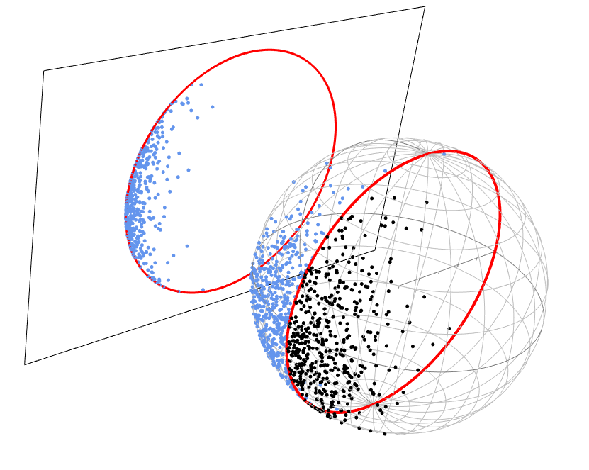
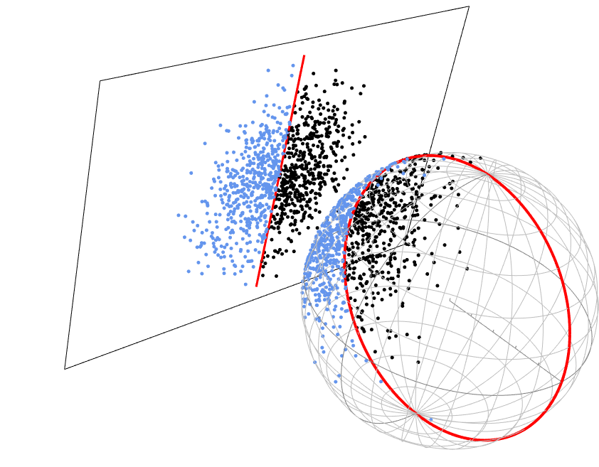
Figure 1: Visualisations of the Euclidean projection, projecting across a different axis, with simulated points from a von Mises-Fisher distribution. A boundary is visualised in red, the unobserved (truncated) points in black and the observed (non-truncated) points in blue. For the projected Euclidean method, $g(\boldsymbol{x})$ is calculated as a 2D Euclidean distance on this projected plane.

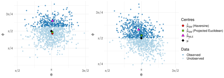
Figure 2: Example of estimation for the von Mises-Fisher distribution (left) and Kent distribution (right), where truncation happens at a constant line of colatitude ($\phi$). The estimated mean directions across both cases is given for different methods, and the different distance functions as described in sections 3.2.1 and 3.2.2.

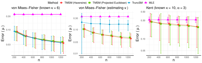
Figure 3: Root mean squared error (with standard deviation), on a log scale, from 512 replicates between the estimates of parameters and the true parameter values, against sample size for each method. Each plot shows a different experiment, from left to right: von Mises-Fisher distribution with known $\kappa$, von Mises-Fisher distribution with unknown $\kappa$ to be estimated, then Kent distribution with known $\kappa$ and $\alpha$.

The points on the surface of the sphere $\boldsymbol{x}\in\mathbb{R}^{3}$ as well as the boundary $\partial M$ can be projected on a two dimensional plane in $\mathbb{R}^{2}$ via setting the third coordinate to zero. Suppose the truncated region is a hemisphere; then the projected plane would be a disk in $\mathbb{R}^{2}$, with the boundary being the outer edge of the disk. See Figure 1 for a visualisation of this method. The corresponding two-dimensional Euclidean distance will be measured on this plane. For the projected point $\boldsymbol{x}_{e}\in\mathbb{R}^{2}$, the distance is given by

$$g(\boldsymbol{x})=\left\lVert\boldsymbol{x}_{e}-\boldsymbol{\tilde{x}}_{e}\right\rVert_{2},$$

where $\boldsymbol{\tilde{x}}_{e}=\operatorname*{arg\,min}_{\boldsymbol{x}_{e}^{\prime}}\left\lVert\boldsymbol{x}_{e}-\boldsymbol{x}_{e}^{\prime}\right\rVert_{2}$ such that $\boldsymbol{x}_{e}^{\prime}\in\partial M$. The gradient is easily defined as

$$\boldsymbol{\nabla}_{\boldsymbol{x}}g(\boldsymbol{x})=\frac{\boldsymbol{x}_{e}-\boldsymbol{\tilde{x}}_{e}}{\left\lVert\boldsymbol{x}_{e}-\boldsymbol{\tilde{x}}_{e}\right\rVert_{2}},$$

i.e. the unit direction away from the boundary.

4 Experiments

We focus on the spheres $S^{2}$ in $\mathbb{R}^{3}$, as this manifold covers many important applications in geological or earth science applications where the datasets are collected from a truncated region on a sphere (Earth).

4.1 Simulated Experiment

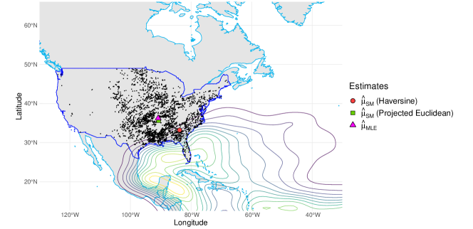
Figure 4: Observed storms as recorded by the USA from 2017 to 2020, with a kernel density estimate contour of storm origin locations over the Atlantic ocean. The mean direction is estimated by TMSM ($\hat{\mu}_{\text{SM}}$) and a maximum likelihood estimate ($\hat{\mu}_{\text{MLE}}$) for comparison.

We start with a synthetic data experiment, where data are simulated from a von Mises-Fisher distribution and Kent distribution using a rejection sampling algorithm, as recommended by Wood (1994). For the von Mises-Fisher distribution experiments, samples are taken with an unknown true mean direction $\boldsymbol{\mu}^{*}=(\pi/2,\pi)$ and an unknown concentration parameter $\kappa^{*}=6$. For the Kent distribution experiments, samples are taken with an unknown true mean direction $\boldsymbol{\mu}^{*}=(\pi/2,\pi)$ and a known concentration parameter and ovalness parameter, $\kappa^{*}=10$ and $\alpha^{*}=3$. The primary aim of estimation in both cases is to produce an estimate for the mean direction, $\boldsymbol{\hat{\mu}}$ and in the von-Mises Fisher case, also an estimate for the concentration, $\hat{\kappa}$.

Figure 2 shows the truncated manifold score matching estimator for the von Mises-Fisher and Kent distribution, where the truncation boundary is at a constant value of colatitude $\phi$. We show estimation results for using the two proposed scaling functions $g(\boldsymbol{x})$; the Haversine distance and projected Euclidean distance. These results are compared against a standard MLE approach, without accounting for the truncation. These plots show even with half of the observations missing, the estimates of the proposed methods are closer to the true mean direction.

4.2 Estimation Accuracy

We repeat experiments to those presented in Section 4.1 across different setups. In each replicate, $n$ samples were simulated from either the von Mises-Fisher or Kent distribution, but only those where the colatitude $\phi>\pi/2$ were observed. Figure 3 shows the root mean squared error, $\frac{1}{d}\sqrt{\sum^{d}_{j=1}(\hat{\mu}_{j}-\mu_{j}^{*})^{2}}$, for different estimates $\boldsymbol{\hat{\mu}}$, plotted as a function of increasing sample size $n$. Each method is as follows: the previous state-of-the-art, Truncated Score Matching, TruncSM Liu et al. (2022), with a multivariate Normal assumption (see appendix B), our method Truncated Manifold Score Matching (TMSM) using either the Haversine or projected Euclidean as $g$, as well as MLE for a baseline.

As expected, in all cases the error decreases as sample size increases, showing empirical consistency. Comparing the two distance functions for $g(\boldsymbol{x})$, both give near identical results across all benchmarks. Our method achieves comparable performance to TruncSM in the first experiment. When $\kappa$ is also estimated, TMSM is clearly superior to TruncSM.

4.3 Storm Events in the USA

Consider an application of estimating the probable locations of extreme storm events in the United States of America (USA) (National Climatic Data Center & of Commerce, 2022). Whilst storms are not restricted to land, observations of these events only happen on land and within the country’s borders. Furthermore, the large area spanned by the USA is significant enough that the curvature of its surface will affect any estimation, highlighting the need for considering estimating densities on a manifold.

We hypothesise that more storms are likely to occur on the East Coast of the USA, and spread across the land from there. We assume there is a true storm ‘centre’ where most storms will be spread out from beyond the country’s eastern border (Oliver, 2008).

Assuming the data can be modelled accurately by a von Mises-Fisher distribution, we estimate the mean direction $\boldsymbol{\mu}$. The estimates $\boldsymbol{\hat{\mu}}$ for both MLE and generalised manifold score matching estimation are given in Figure 4. Included in the figure is a kernel density estimate of storm points of origin, which are calculated via a post-storm analysis, after a storm is observed Landsea & Franklin (2013). Not surprisingly, we see that $\boldsymbol{\hat{\mu}}$ given by MLE is at the center of the dataset, whereas the truncated manifold score matching estimate is further South East, closer to the storm origins.

5 Discussion

The aim of this work was to derive an estimator for truncated densities on a generic manifold. We applied Stokes’ theorem and a scaling function to obtain a tractable score matching objective, of which the estimation was possible via numerical minimisation. The method was tested on the two dimensional sphere in $\mathbb{R}^{3}$, where we showed a superior performance comparing to a Euclidean approximation using TruncSM. A further application was presented on severe storms in the USA, in which the score matching estimator gave a mean direction estimate lying on the East Coast, where the bulk of the storms originated.

Our estimator should also be applicable to any manifold in which Stokes’ Theorem holds, but applications have only been studied on the two dimensional sphere. Other complicated manifolds would require different distribution specification and different scaling functions. It is likely there exists a general purpose scaling function on a manifold that involves projection into a Euclidean domain, which could generalise this work further, but it is beyond the scope of this work.

Software and Data

A fully packaged implementation in R, with examples and a tutorial, can be found at the GitHub repository here: https://github.com/dannyjameswilliams/truncsm.

Appendix A Proof of Theorem 3.1

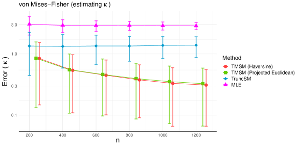
Figure 5: Root mean squared error (with standard deviation) from 512 replicates between $\kappa^{*}=6$ and the estimated $\hat{\kappa}$ given by the different methods.

Proof.

We can expand out (13) to give

$$J_{S}(\boldsymbol{\beta})=\int_{M}q(\boldsymbol{x})g(\boldsymbol{x})\Big{[}\langle\boldsymbol{\nabla}_{\boldsymbol{x}}\log p(\boldsymbol{x};\boldsymbol{\beta}),\boldsymbol{\nabla}_{\boldsymbol{x}}\log p(\boldsymbol{x};\boldsymbol{\beta})\rangle_{M}-2\langle\boldsymbol{\nabla}_{\boldsymbol{x}}\log p(\boldsymbol{x};\boldsymbol{\beta}),\boldsymbol{\nabla}_{\boldsymbol{x}}\log q(\boldsymbol{x})\rangle_{M}\Big{]}d\boldsymbol{x}+C_{q},$$

where $C_{q}=\int_{M}q(\boldsymbol{x})g(\boldsymbol{x})\langle\boldsymbol{\nabla}_{\boldsymbol{x}}\log q(\boldsymbol{x}),\boldsymbol{\nabla}_{\boldsymbol{x}}\log q(\boldsymbol{x})\rangle_{M}d\boldsymbol{x}$ does not depend on $\boldsymbol{\beta}$, and can be ignored as minimisation would return the same result regardless of its inclusion. Expanding the second term gives

$$\int_{M}g(\boldsymbol{x})q(\boldsymbol{x})\langle\boldsymbol{\nabla}_{\boldsymbol{x}}\log p(\boldsymbol{x};\boldsymbol{\beta}),\boldsymbol{\nabla}_{\boldsymbol{x}}\log q(\boldsymbol{x})\rangle_{M}d\boldsymbol{x}=\int_{M}g(\boldsymbol{x})\langle\boldsymbol{\nabla}_{\boldsymbol{x}}\log p(\boldsymbol{x};\boldsymbol{\beta}),\boldsymbol{\nabla}_{\boldsymbol{x}}q(\boldsymbol{x})\rangle_{M}d\boldsymbol{x},$$

due to the identity that $\partial\log q(\boldsymbol{x})/\partial x_{i}=(q(\boldsymbol{x}))^{-1}\partial q(\boldsymbol{x})/\partial x_{i}$. We can apply Theorem 2.1 to this term, noting that $f_{1}=g(\boldsymbol{x})q(\boldsymbol{x})$ and $f_{2}=\log p(\boldsymbol{x};\boldsymbol{\beta})$, on our manifold $M$ with boundary $\partial M$, then

$$\oint_{\partial M}g(\boldsymbol{x})q(\boldsymbol{x})\frac{\partial\boldsymbol{\nabla}_{\boldsymbol{x}}\log p(\boldsymbol{x};\boldsymbol{\beta})}{\partial\mathbf{n}}\partial M =\int_{M}(\boldsymbol{\Delta}_{M}\log p(\boldsymbol{x};\boldsymbol{\beta}))g(\boldsymbol{x})q(\boldsymbol{x})d\boldsymbol{x}$$

$$+\int_{M}\langle\boldsymbol{\nabla}_{\boldsymbol{x}}g(\boldsymbol{x})q(\boldsymbol{x}),\boldsymbol{\nabla}_{\boldsymbol{x}}\log p(\boldsymbol{x};\boldsymbol{\beta})\rangle_{M}d\boldsymbol{x}$$

where $\mathbf{n}$ is the unit normal vector. Since we construct $g(\boldsymbol{x}^{\prime})=0$ on all points $\boldsymbol{x}^{\prime}\in\partial M$ then the term on the left hand side vanishes to zero. This step is critical, and why it is necessary for the condition on $g$. The terms on the right hand side can be expanded via the chain rule and rearranged to

$$\int_{M}g(\boldsymbol{x})\langle\boldsymbol{\nabla}_{\boldsymbol{x}}\log p(\boldsymbol{x};\boldsymbol{\beta}),\boldsymbol{\nabla}_{\boldsymbol{x}}q(\boldsymbol{x})\rangle_{M}d\boldsymbol{x}= -\int_{M}q(\boldsymbol{x})g(\boldsymbol{x})(\boldsymbol{\Delta}_{M}\log p(\boldsymbol{x};\boldsymbol{\beta}))d\boldsymbol{x}$$

$$-\int_{M}q(\boldsymbol{x})\langle\boldsymbol{\nabla}_{\boldsymbol{x}}g(\boldsymbol{x}),\boldsymbol{\nabla}_{\boldsymbol{x}}\log p(\boldsymbol{x};\boldsymbol{\beta})\rangle_{M}d\boldsymbol{x},$$

where $\boldsymbol{\Delta}_{M}$ is the Laplace-Beltrami operator. The term on the left hand side can be substituted into $J_{S}(\boldsymbol{\beta})$ to obtain

$$J_{S}(\boldsymbol{\beta}) =\int_{M}q(\boldsymbol{x})g(\boldsymbol{x})\langle\boldsymbol{\nabla}_{\boldsymbol{x}}\log p(\boldsymbol{x};\boldsymbol{\beta}),\boldsymbol{\nabla}_{\boldsymbol{x}}\log p(\boldsymbol{x};\boldsymbol{\beta})\rangle_{M}d\boldsymbol{x}+2\int_{M}q(\boldsymbol{x})g(\boldsymbol{x})\boldsymbol{\Delta}_{M}\log p(\boldsymbol{x};\boldsymbol{\beta})d\boldsymbol{x}$$

$$\qquad\qquad\qquad\qquad\qquad\qquad+2\int_{M}q(\boldsymbol{x})\langle\boldsymbol{\nabla}_{\boldsymbol{x}}g(\boldsymbol{x}),\boldsymbol{\nabla}_{\boldsymbol{x}}\log p(\boldsymbol{x};\boldsymbol{\beta})\rangle_{M}d\boldsymbol{x},$$

which gives the desired result. ∎

Appendix B Notes on Benchmarks from Section 4.2

In the first two experiments from Section 4.2, and the left two plots from Figure 3, the task was estimating the mean direction $\boldsymbol{\mu}$ in the von Mises-Fisher distribution when the concentration parameter, $\kappa$, was known and unknown. Whilst the truncated manifold score matching methods can estimate $\kappa$ directly, for TruncSM we let $\boldsymbol{\mu}_{\text{MVN}}=\boldsymbol{\mu}_{\boldsymbol{z}}$, i.e. the mean of the MVN distribution is the mean direction of the von Mises-Fisher distribution in polar coordinates, and $\boldsymbol{\Sigma}_{\text{MVN}}=\kappa^{-1}\mathbf{I}_{d}$, i.e. the covariance matrix of the MVN is isotropic. In this case, we treat $\kappa^{-1}$ as the precision parameter and estimate it directly with the TruncSM formulation. Figure 5 shows a similar benchmark plot, giving the error for estimating $\kappa$, this plot is parallel to the middle-most plot in Figure 3.

Whilst there is a clear difference between the errors for estimation from TruncSM and truncated manifold score matching in both Figures 3 and 5, it is clear from the first experiment, where $\kappa$ is known, that the equality $\boldsymbol{\Sigma}_{\text{MVN}}=\kappa^{-1}\mathbf{I}_{d}$ holds, since the methods were very close in performance when $\kappa^{-1}=1/6$ was fixed..

References

- Hyvärinen (2005) Hyvärinen, A. Estimation of non-normalized statistical models by score matching. Journal of Machine Learning Research, 6(Apr):695–709, 2005.
- Hyvärinen (2007) Hyvärinen, A. Some extensions of score matching. Computational statistics & data analysis, 51(5):2499–2512, 2007.
- Kent (1982) Kent, J. T. The fisher-bingham distribution on the sphere. Journal of the Royal Statistical Society: Series B (Methodological), 44(1):71–80, 1982.
- Landsea & Franklin (2013) Landsea, C. W. and Franklin, J. L. Atlantic hurricane database uncertainty and presentation of a new database format, 2013. Mon. Wea. Rev., 141, 3576-3592. Date accessed: 10th May 2022.
- Lee (2013) Lee, J. M. Smooth manifolds. In Introduction to Smooth Manifolds, pp. 1–31. Springer, 2013.
- Li (2009) Li, S. Z. Markov random field modeling in image analysis. Springer Science & Business Media, 2009.
- Lin et al. (2016) Lin, L., Drton, M., and Shojaie, A. Estimation of high-dimensional graphical models using regularized score matching. Electronic journal of statistics, 10(1):806, 2016.
- Liu et al. (2022) Liu, S., Kanamori, T., and Williams, D. J. Estimating density models with truncation boundaries using score matching. arXiv preprint, arXiv:1910.03834, 2022.
- Mardia & Jupp (2009) Mardia, K. V. and Jupp, P. E. Directional statistics, 2009.
- Mardia et al. (2016) Mardia, K. V., Kent, J. T., and Laha, A. K. Score matching estimators for directional distributions. arXiv preprint arXiv:1604.08470, 2016.
- National Climatic Data Center & of Commerce (2022) National Climatic Data Center, NESDIS, N. and of Commerce, U. D. Ncdc storm events database, 2022. Date accessed: 10th May 2022.
- Oliver (2008) Oliver, J. E. Encyclopedia of world climatology. Springer Science & Business Media, 2008.
- Papadakis et al. (2021) Papadakis, M., Tsagris, M., Dimitriadis, M., Fafalios, S., Tsamardinos, I., Fasiolo, M., Borboudakis, G., Burkardt, J., Zou, C., Lakiotaki, K., and Chatzipantsiou., C. Rfast: A Collection of Efficient and Extremely Fast R Functions, 2021. URL https://CRAN.R-project.org/package=Rfast. R package version 2.0.3.
- R Core Team (2021) R Core Team. R: A Language and Environment for Statistical Computing. R Foundation for Statistical Computing, Vienna, Austria, 2021. URL https://www.R-project.org/.
- Stewart et al. (2020) Stewart, J., Clegg, D. K., and Watson, S. Calculus: early transcendentals. Cengage Learning, 2020.
- Teh et al. (2003) Teh, Y. W., Welling, M., Osindero, S., and Hinton, G. E. Energy-based models for sparse overcomplete representations. Journal of Machine Learning Research, 4(Dec):1235–1260, 2003.
- Tsagris et al. (2021) Tsagris, M., Athineou, G., Sajib, A., Amson, E., and Waldstein, M. J. Directional: A Collection of R Functions for Directional Data Analysis, 2021. URL https://CRAN.R-project.org/package=Directional. R package version 5.0.
- Wickham (2016) Wickham, H. ggplot2: Elegant Graphics for Data Analysis. Springer-Verlag New York, 2016. ISBN 978-3-319-24277-4. URL https://ggplot2.tidyverse.org.
- Wood (1994) Wood, A. T. Simulation of the von mises fisher distribution. Communications in statistics-simulation and computation, 23(1):157–164, 1994.
- Yu et al. (2016) Yu, M., Kolar, M., and Gupta, V. Statistical inference for pairwise graphical models using score matching. pp. 2829–2837, 2016.
- Yu et al. (2019) Yu, S., Drton, M., and Shojaie, A. Generalized score matching for non-negative data. Journal of Machine Learning Research, 20(76):1–70, 2019. URL http://jmlr.org/papers/v20/18-278.html.
- Yu et al. (2021) Yu, S., Drton, M., and Shojaie, A. Generalized score matching for general domains. Information and Inference: A Journal of the IMA, 01 2021.