Cut Inner Layers: A Structured Pruning Strategy for Efficient U-Net GANs

Bo-Kyeong Kim Shinkook Choi Hancheol Park

Abstract

Pruning effectively compresses overparameterized models. Despite the success of pruning methods for discriminative models, applying them for generative models has been relatively rarely approached. This study conducts structured pruning on U-Net generators of conditional GANs. A per-layer sensitivity analysis confirms that many unnecessary filters exist in the innermost layers near the bottleneck and can be substantially pruned. Based on this observation, we prune these filters from multiple inner layers or suggest alternative architectures by completely eliminating the layers. We evaluate our approach with Pix2Pix for image-to-image translation and Wav2Lip for speech-driven talking face generation. Our method outperforms global pruning baselines, demonstrating the importance of properly considering where to prune for U-Net generators.

Structured Pruning, U-Net, Generative Adversarial Network, GAN

1 Introduction

Developing lightweight neural networks has attracted considerable attention for their efficient deployment in real-world applications. A popular method for network compression is pruning (LeCun et al., 1989; Wen et al., 2016), which removes unimportant weights from overparameterized models. Numerous studies have successfully applied pruning methods for discriminative models (e.g., image classifiers (Frankle & Carbin, 2019; Ning et al., 2020; Yeom et al., 2021) and object detectors (Shih et al., 2019; Ghosh et al., 2019; Xie et al., 2020)); however, applying them for generative models has been relatively less investigated.

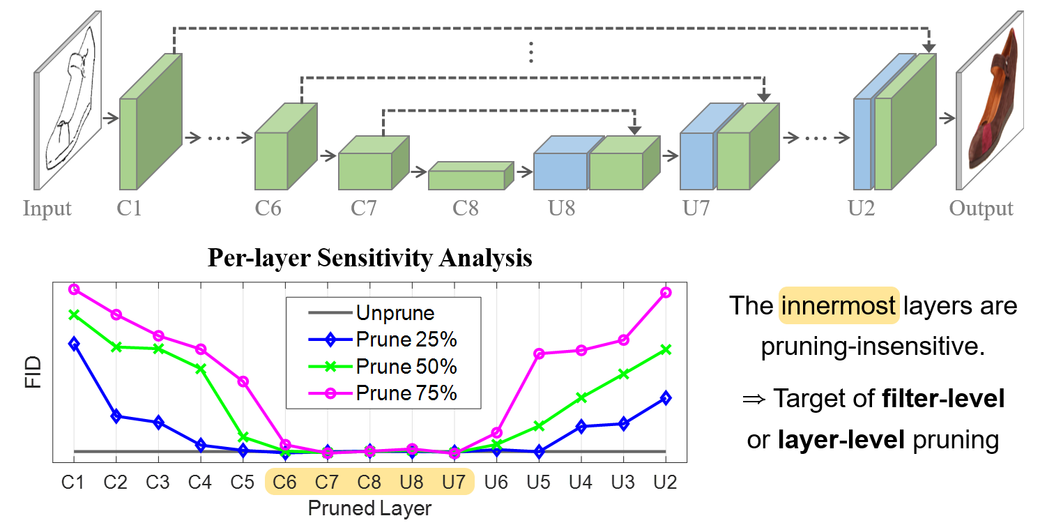
Refer to caption — Figure 1: Illustration of (top) a U-Net generator and (bottom) a per-layer pruning sensitivity analysis. A lower FID indicates a better generation quality. The analysis reveals that the innermost layers in U-Net generators have many unimportant filters, which can be pruned without noticeable performance degradation.

In this study, we focus on pruning of U-Net (Ronneberger et al., 2015) generators that have been widely used in generative adversarial networks (GANs) (Goodfellow et al., 2014) for conditional image synthesis tasks (Yang et al., 2020; Isola et al., 2017; Prajwal et al., 2020). As shown in Figure 1, a U-Net consists of an encoder and a decoder, where skip connections shuttle context information across the network. It contains a huge number of parameters, all of which may not be necessary for high-fidelity image generation. Through pruning, we not only compress the generator but also deepen our understanding on the network behavior.

A layer-wise sensitivity analysis for understanding how pruning of each layer affects the performance has been conducted merely on classification models (Ning et al., 2020; Li et al., 2017; Lin et al., 2019). Applying such an analysis for GANs is arguably more challenging because of the difficulty in retraining and evaluating pruned generators. To the best of our knowledge, this is the first attempt to analyze the pruning sensitivity of GAN generators. Our analysis reveals that many filters in the innermost layers of the U-Net are redundant and can be removed. We observe this phenomenon consistently with different datasets, network capacities, pruning criteria, and evaluation metrics.

Based on the analysis, we perform filter pruning of multiple innermost layers or even remove these layers entirely. We evaluate our approach for the U-Net generator of Pix2Pix (Isola et al., 2017) on the Edges2Shoes (Yu & Grauman, 2014) and Facades (Tyleček & Šára, 2013) datasets and for that of Wav2Lip (Prajwal et al., 2020) on the LRS3 dataset (Afouras et al., 2018). Our method outperforms global pruning baselines that are commonly used for classification models, indicating that properly considering where to prune for the U-Net is important.

2 Related Work

Although there have been several studies for learning efficient GANs (e.g., using neural architecture search (Gao et al., 2020; Gong et al., 2019; Fu et al., 2020; Hou et al., 2021) or network quantization (Wang et al., 2020, 2019; Wan et al., 2020; Andreev et al., 2021)), we mainly discuss pruning-based approaches that are often combined with knowledge distillation (KD) (Hinton et al., 2014; Romero et al., 2015) to improve the performance.

In the KD setups of Li et al. (2022, 2021); Jin et al. (2021); Liu et al. (2021); Li et al. (2020), pruned generators that act as students are trained under the guidance of original large generators that act as teachers. To derive pruned models, they inject sparsity constraints during training the original generator (Li et al., 2022, 2021) or redesign the original model to provide an architectural search space (Jin et al., 2021); however, these methods become difficult or impossible to apply when the compression of already pretrained generators is needed. We consider a practical case for pruning of pretrained GANs obtained without sparsity regularization or redesigning steps.

Instead of using pruned generators as the initialization of students (Li et al., 2021; Jin et al., 2021; Liu et al., 2021), some studies (Wang et al., 2020; Shu et al., 2019) infer compressed student architectures during the KD process. Unstructured pruning has also been applied to compress GANs with the lottery ticket hypothesis (Chen et al., 2021b, a) or with a KD strategy (Yu & Pool, 2020).

Method Large Generator (nF=64) Small Generator (nF=32) Category Bottleneck Pruned Layer/Ratio FID (↓) #Params MACs FID (↓) #Params MACs Original Pix2Pix 1×1 - 29.0 54.4M 18.14G 43.5 13.6M 4.65G Global Pruning Uniform 1×1 All Layers/1% 33.5 53.4M 17.88G 43.9 13.4M 4.61G 1×1 All Layers/2% 59.3 52.3M 17.51G 46.6 13.1M 4.52G Uniform+ (Gale et al., 2019) 1×1 All Layers Except C1 & U2/2% 38.7 52.3M 17.59G 46.6 13.1M 4.52G 1×1 All Layers Except C1 & U2/3% 41.1 51.3M 17.33G 48.0 12.9M 4.48G Structured LAMP (Lee et al., 2021) 1×1 LAMP-based Selection/1% 47.0 53.4M 16.78G 66.8 13.4M 4.35G 1×1 LAMP-based Selection/2% 75.9 52.4M 15.39G 118.3 13.1M 4.02G Ours Filter Pruning 1×1 {C6-C7-C8}/50% 30.4 39.7M 17.92G 43.7 9.9M 4.59G 1×1 {C6-C7-C8}/50% + {U8-U7}/25% 31.9 35.8M 17.81G 44.4 9.0M 4.57G Layer Removal 2×2 {C8-U8}/100% 28.3 41.8M 18.06G 39.9 10.5M 4.63G 4×4 {C7-C8-U8-U7}/100% 29.7 29.2M 17.70G 41.9 7.3M 4.54G

Table 1: Quantitative results on the Edges2Shoes (edges→photo) dataset. The models marked in bold face provide a good performance-efficiency trade-off (see Figure 4(a) for their visual results).

Method Large Generator (nF=64) Small Generator (nF=32) Category Bottleneck Pruned Layer/Ratio FID (↓) #Params MACs FID (↓) #Params MACs Original Pix2Pix 1×1 - 115.3 54.4M 18.14G 124.0 13.6M 4.65G Global Pruning Uniform 1×1 All Layers/2% 118.1 52.3M 17.51G 128.4 13.1M 4.52G 1×1 All Layers/4% 127.9 50.2M 16.81G 139.1 12.6M 4.33G Uniform+ (Gale et al., 2019) 1×1 All Layers Except C1 & U2/2% 119.4 52.3M 17.59G 128.4 13.1M 4.52G 1×1 All Layers Except C1 & U2/4% 123.4 50.3M 16.97G 135.3 12.6M 4.37G Structured LAMP (Lee et al., 2021) 1×1 LAMP-based Selection/4% 115.2 50.6M 18.11G 127.1 12.6M 4.57G 1×1 LAMP-based Selection/6% 118.9 48.2M 17.75G 127.6 12.0M 4.49G Ours Filter Pruning 1×1 C6/50% + {C7-C8-U8-U7}/75% 113.2 27.7M 17.61G 124.7 6.9M 4.52G 1×1 C6/50% + {C7-C8-U8-U7}/75% + U6/25% 114.0 25.8M 17.30G 125.3 6.5M 4.44G Layer Removal 2×2 {C8-U8}/100% 107.9 41.8M 18.06G 108.5 10.5M 4.63G 4×4 {C7-C8-U8-U7}/100% 108.7 29.2M 17.70G 108.9 7.3M 4.54G

Table 2: Quantitative results on the Facades (architectural labels→photo) dataset. The models marked in bold face provide a good performance-efficiency trade-off (see Figure 4(b) for their visual results).

Method Performance Computation Latency (ms / 16 frames) FID (↓) LSE-D (↓) LSE-C (↑) # Params MACs CPU GPU Wav2Lip Original 6.16 6.50 7.44 36.3M (1.0×) 6.21G (1.0×) 1111.5 (1.0×) 24.8 (1.0×) Compressed Generator 6.15 6.92 7.17 5.0M (7.2×) 0.84G (7.4×) 200.2 (5.6×) 7.4 (3.4×) Global Pruning Uniform (9%) ${}^{\textrm{a}}$ 11.62 7.62 6.19 4.2M (8.7×) 0.72G (8.7×) 170.6 (6.5×) 6.9 (3.6×) Uniform (38%) ${}^{\textrm{b}}$ 28.31 7.82 5.74 1.9M (18.7×) 0.33G (18.7×) 107.3 (10.4×) 4.3 (5.7×) Structured LAMP (Lee et al., 2021) (36%) ${}^{\textrm{a,b}}$ 8.23 7.53 6.33 2.0M (18.3×) 0.71G (8.7×) 167.6 (6.6×) 6.3 (3.9×) Ours Filter Pruning ${}^{\textrm{c}}$ 6.09 7.29 6.61 1.9M (18.9×) 0.70G (8.9×) 164.3 (6.8×) 6.2 (4.0×) a Similar MACs with ours. b Similar number of parameters with ours. c Filter pruning of the innermost layers: 50% filters of { $\mathrm{C^{A}}$ 5-6-7, $\mathrm{C^{V}}$ 6-7-8, $\mathrm{U}$ 6-5} and 67% filters of $\mathrm{U4}$ are removed.

Table 3: Quantitative results on the LRS3 dataset. The latency was measured on Xeon Silver 4114 CPU or RTX 2080 Ti GPU. ↑ and ↓ indicate that higher and lower values are better, respectively. The pruning ratio used in global pruning is provided in parentheses.

3 Method

3.1 Magnitude-based Pruning Criterion

We primarily use a criterion based on weight magnitude for filter pruning. $\mathcal{F}\in\mathbb{R}^{n_{in}\times n_{out}\times k\times k}$ represents the kernel matrix of a convolutional layer, where $n_{in}$ , $n_{out}$ , and $k$ denote the number of input and output channels and the spatial kernel size, respectively. For the $i$ -th filter, $\mathcal{F}_{i}\in\mathbb{R}^{n_{in}\times k\times k}$ , its $L$ 2-norm magnitude $\|\mathcal{F}_{i}\|_{2}$ is used as an importance score. Because filters with smaller weight magnitudes cause low activation feature maps, removing these filters tends to exhibit little or no performance degradation. In Section 5.4, we also investigate another criterion based on the redundancy in convolutional filters (He et al., 2019).

3.2 Layer-wise Sensitivity Analysis

To identify which layers contain unnecessary filters in the U-Net generator, we prune the filters of each layer independently and observe the generation performance of the pruned network. We vary the pruning ratio of {25%, 50%, 75%} for each layer and repeat this process over all parameterized layers. Such an analysis has been conducted for discriminative models (Ning et al., 2020; Li et al., 2017; Lin et al., 2019); to the best of our knowledge, this is the first layer-wise sensitivity analysis for generative models.

3.3 Filter-level Pruning

The sensitivity analysis confirms that the innermost layers of the U-Net generator have a large number of unimportant filters and are insensitive to pruning. Based on this observation, we prune these filters simultaneously from multiple innermost layers to boost computational efficiency. We determine the layers being pruned and the pruning ratio through a grid search over the innermost layers.

3.4 Layer-level Pruning (Layer Removal)

We also investigate the effect of layer pruning: we remove the innermost layers entirely and make the redesigned network have wider bottleneck dimensions (e.g., 2×2 or 4×4) instead of 1×1. Based on the symmetric architecture of the U-Net, when eliminating the layers of the encoder, we correspondingly remove the mirrored layers of the decoder (e.g., C8 and U8 in Figure 2(a) are removed together).

3.5 Retraining of Pruned Generators

Given a pretrained GAN, we run a single pruning-retraining cycle. Retraining a pruned generator is arguably more tricky than retraining a typical classifier, because of taking the discriminator into account. We finetune the pruned generator while jointly training the pretrained discriminator. In Appendix B, we discuss other retraining settings and present their results.

4 Experimental Setup

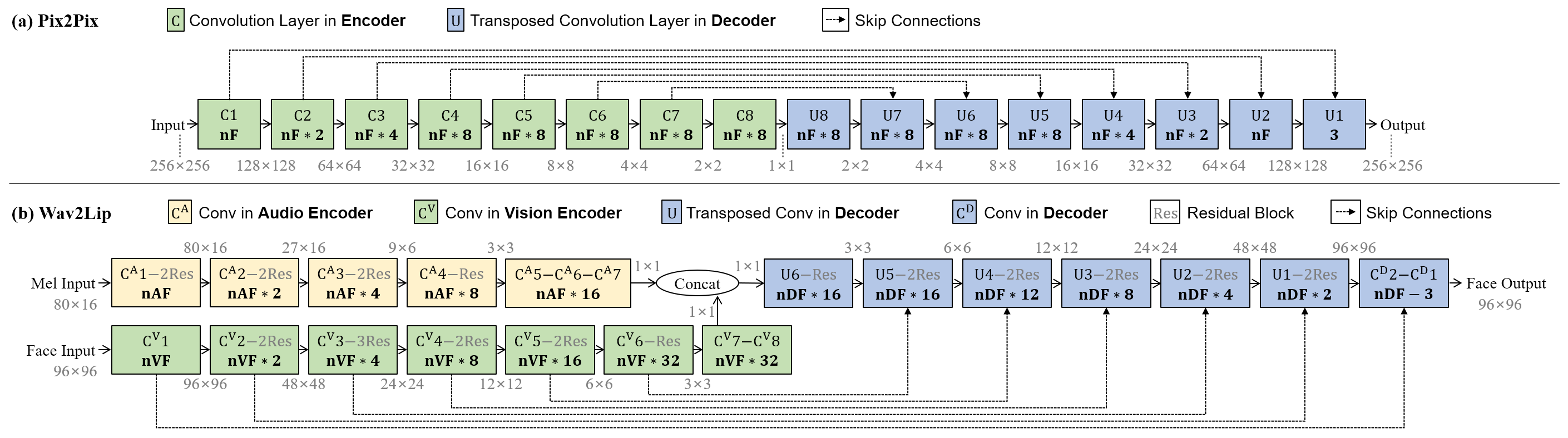
Architecture. Figure 2 depicts the U-Net generators of Pix2Pix (Isola et al., 2017) and Wav2Lip (Prajwal et al., 2020). For Wav2Lip, we build an efficient yet effective generator by halving the number of filters (i.e., ( $\mathrm{nVF}$ , $\mathrm{nAF}$ , $\mathrm{nDF}$ ) changes from (16, 32, 32) to (8, 16, 16)) and removing all the residual blocks. See Appendix A for the details.

Baseline. We compare our method with global pruning approaches to validate the importance of properly considering where to prune in the U-Net. Uniform pruning removes small-magnitude filters of every layer with a given pruning ratio. Uniform+ pruning is almost identical to Uniform, except that the first encoder layer and the last decoder layer are not pruned. This is similar to the heuristic suggested in Gale et al. (2019) for classification models. Moreover, we modify Layer-Adaptive Magnitude-based Pruning (LAMP) (Lee et al., 2021), which was originally unstructured pruning, to perform structured pruning and call it Structured LAMP.

Dataset. For Pix2Pix, we consider the Edges2Shoes (Yu & Grauman, 2014) and Facades (Tyleček & Šára, 2013) datasets that contain 50K and 0.5K images, respectively. We follow the training and test data splits of Isola et al. (2017). For Wav2Lip, we use the LRS3 dataset (Afouras et al., 2018) that contains 32K utterances from 4K speakers of TED videos. We train and evaluate the models with the original data splits of LRS3.

Evaluation Metric. We adopt Frechet Inception Distance (FID) (Heusel et al., 2017) to assess the generation quality. Moreover, we consider recent metrics to separately evaluate the fidelity and diversity of generated images (Kynkäänniemi et al., 2019; Naeem et al., 2020). For Wav2Lip, we additionally compute Lip Sync Error - Distance (LSE-D) and Confidence (LSE-C) (Chung & Zisserman, 2016) to assess the quality of lip synchronization between speech and generated face samples. We also report the number of parameters and multiply-accumulate operations (MACs)¹¹1Although MACs have been widely used to measure the computational cost, they may lead to an inaccurate energy consumption estimation (Sze et al., 2017)..

Implementation Details. We implement the pruning methods with NetsPresso Model Compressor²²2https://www.netspresso.ai/model-compressor and adopt the publicly available codes of Pix2Pix³³3https://github.com/junyanz/pytorch-CycleGAN-and-pix2pix and Wav2Lip⁴⁴4https://github.com/Rudrabha/Wav2Lip. The optimization settings closely follow the original settings of Isola et al. (2017) and Prajwal et al. (2020) except empirically determining the batch size, the number of training epochs, and the type of GAN loss (see Appendix C for the details). We use a single NVIDIA GeForce RTX 3090 GPU for the training process.

5 Results and Analyses

5.1 Pruning Pix2Pix Models

5.1.1 Layer-wise Sensitivity Analysis

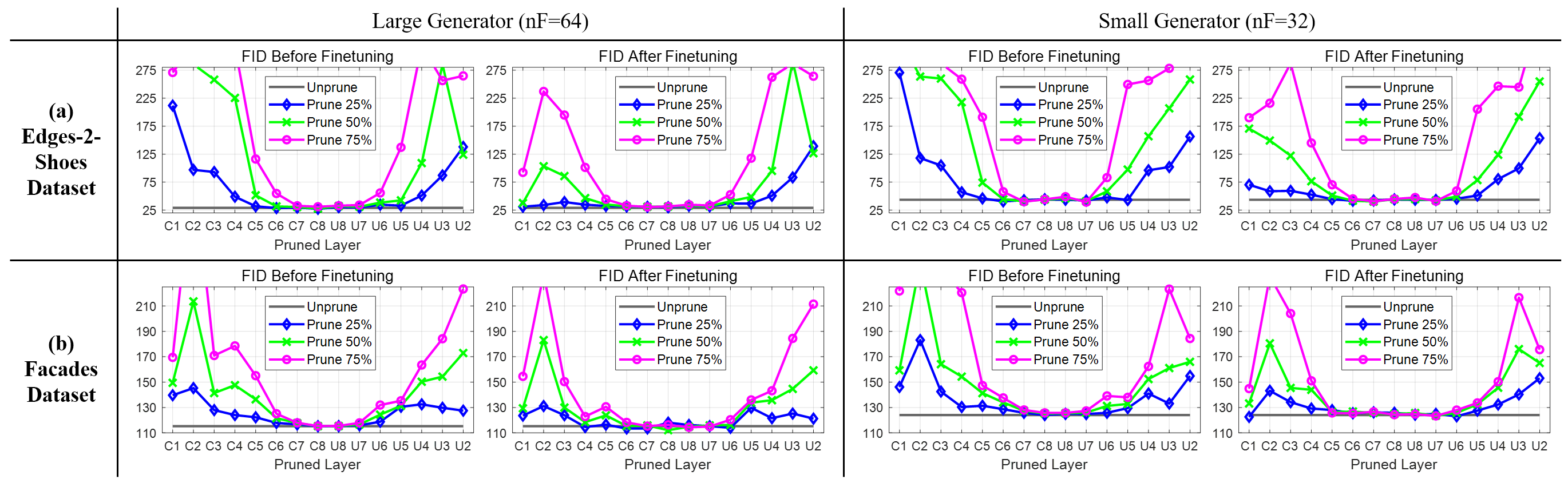
Figure 3 shows the sensitivity analysis. Pruning each of the five innermost layers (i.e., C6, C7, C8, U8, U7) leads to a similar FID score with the original model even at the pruning ratio of 75%, indicating that these layers contain many unnecessary filters and are insensitive to pruning. In contrast, pruning outer layers causes substantial performance drops, confirming that outer layers and their skip connections are essential for the generation tasks. In other words, because of the same underlying structure shared between the input and output, delivering low-level information via outer skip connections is important. This U-shaped trend also appears in the case of a smaller generator capacity.

5.1.2 Filter-level and Layer-level Pruning

Tables 1 and 2 report the quantitative results. For the Edges2Shoes dataset, we were unable to achieve compelling results with the global pruning baselines. Eliminating only 1% or 2% of the filters from every layer with the uniform methods degrades the FID scores. The LAMP method removes many filters in the U4 layer, which is identified as a pruning-sensitive layer in our layer-wise analysis.

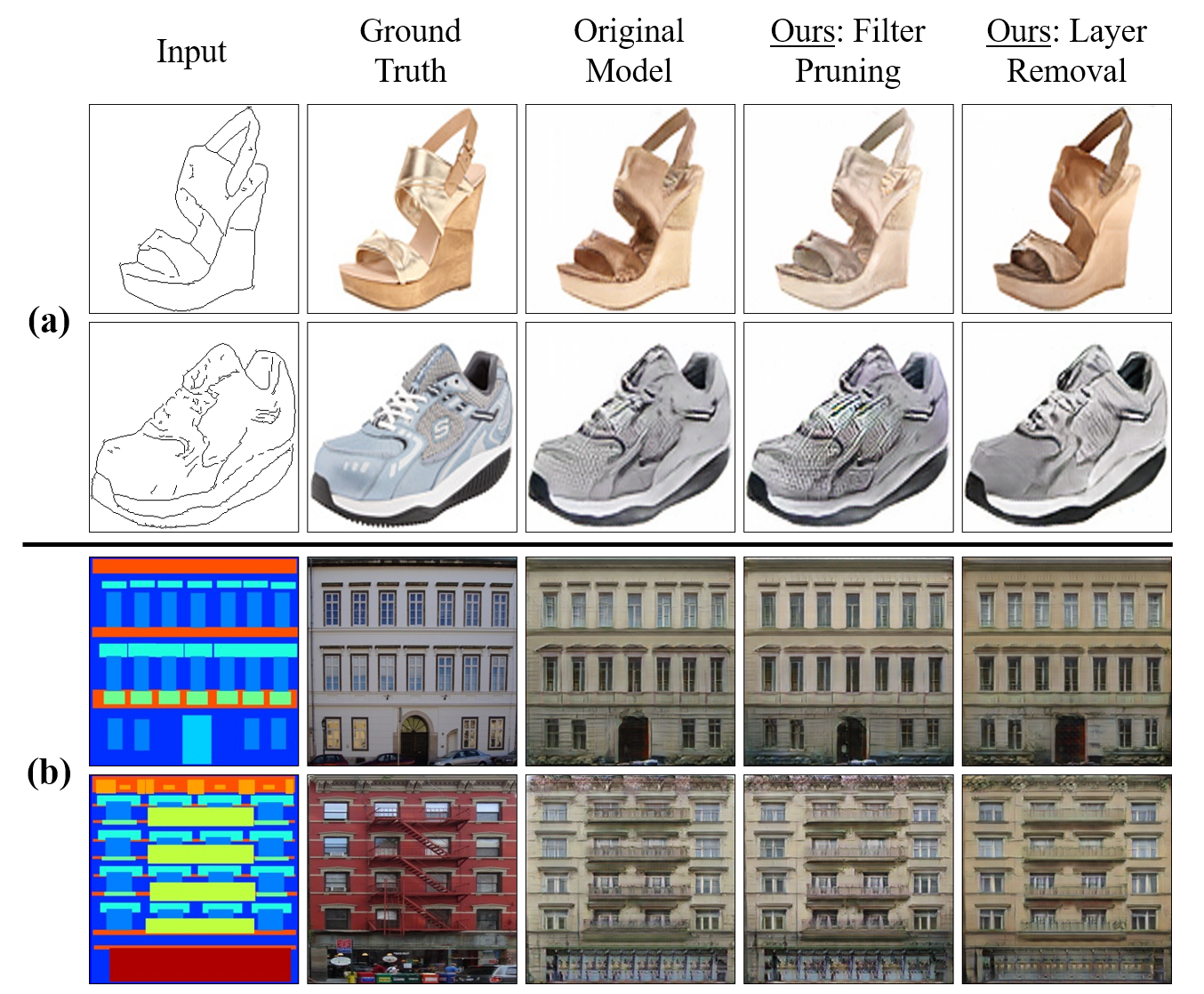
By contrast, filter-level and layer-level pruning of the innermost layers do not exhibit noticeable performance drops while effectively reducing the number of parameters and MACs. These results suggest that properly determining where to prune is important. Interestingly, some pruned networks yield better FID scores than the original networks, which may be connected to the ability of pruning for mitigating overfitting (Hanson & Pratt, 1988) and ablating defective weights (Tousi et al., 2021). Moreover, as shown in Figure 4, our pruned models perform comparatively to the original models in terms of visual fidelity.

5.2 Pruning Wav2Lip Models

From the compressed generator, we prune the filters of the three innermost layers of the vision encoder, audio encoder, and decoder in Figure 2(b). The number of filters in these layers changes from 256 or 192 to 128 after pruning.

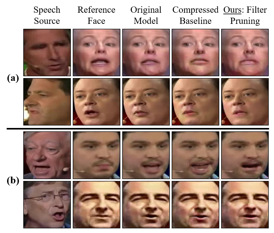
Table 3 shows the quantitative results on the LRS3 dataset. Although the compressed generator was already much more efficient than the original large model, we can further compress it without significant performance degradation. Moreover, our method outperforms the global pruning baselines that have similar computational costs, demonstrating the effectiveness of pruning innermost filters in the U-Net generator. Figure 5 depicts some visual examples. Our method can generate lip-synced face images without loss of visual quality under a reduced computational budget.

5.3 Additional Evaluation Metrics

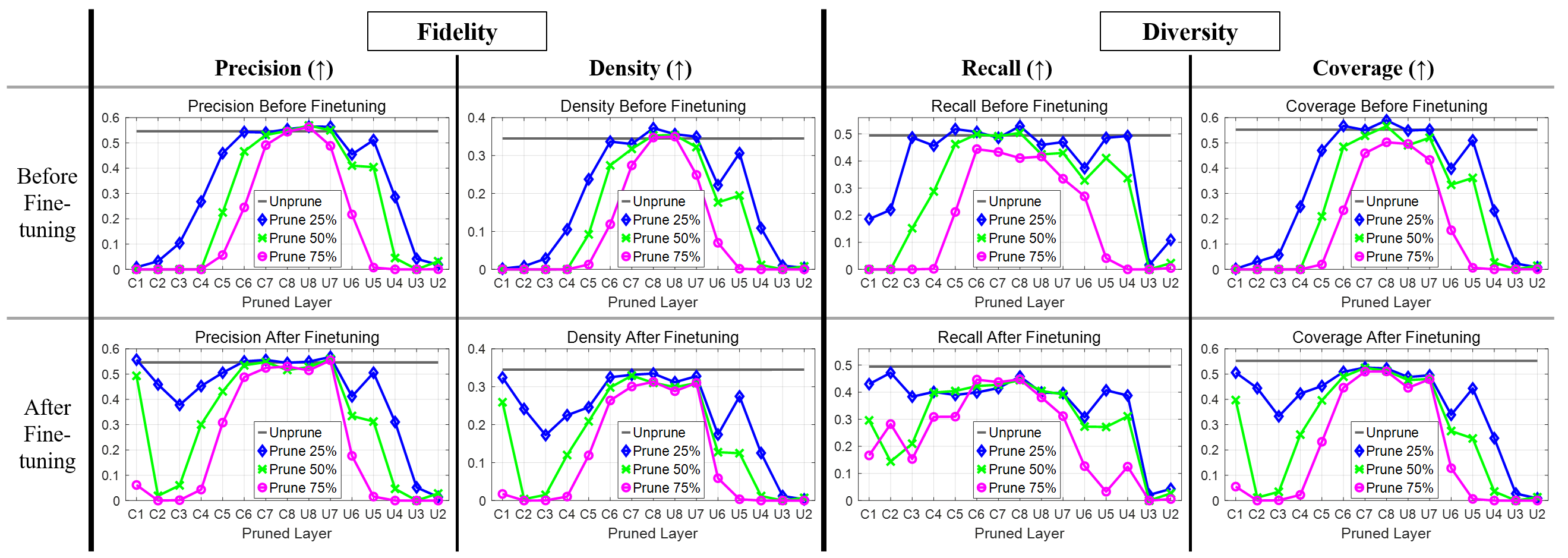
In addition to FID, we further adopt recent metrics (Kynkäänniemi et al., 2019; Naeem et al., 2020) to study how pruning of each layer affects the fidelity and diversity aspects of generated images. Figure 6 shows the results on the Edges2shoes dataset with Pix2Pix. Similarly to Figure 3, filter pruning of the innermost layers better preserves the examined aspects than that of the outer layers. At the severe pruning ratio of 75% before finetuning, pruning innermost filters retains the fidelity but slightly degrades the diversity, which is similarly reported in Mordido et al. (2021).

5.4 Comparison of Pruning Criteria

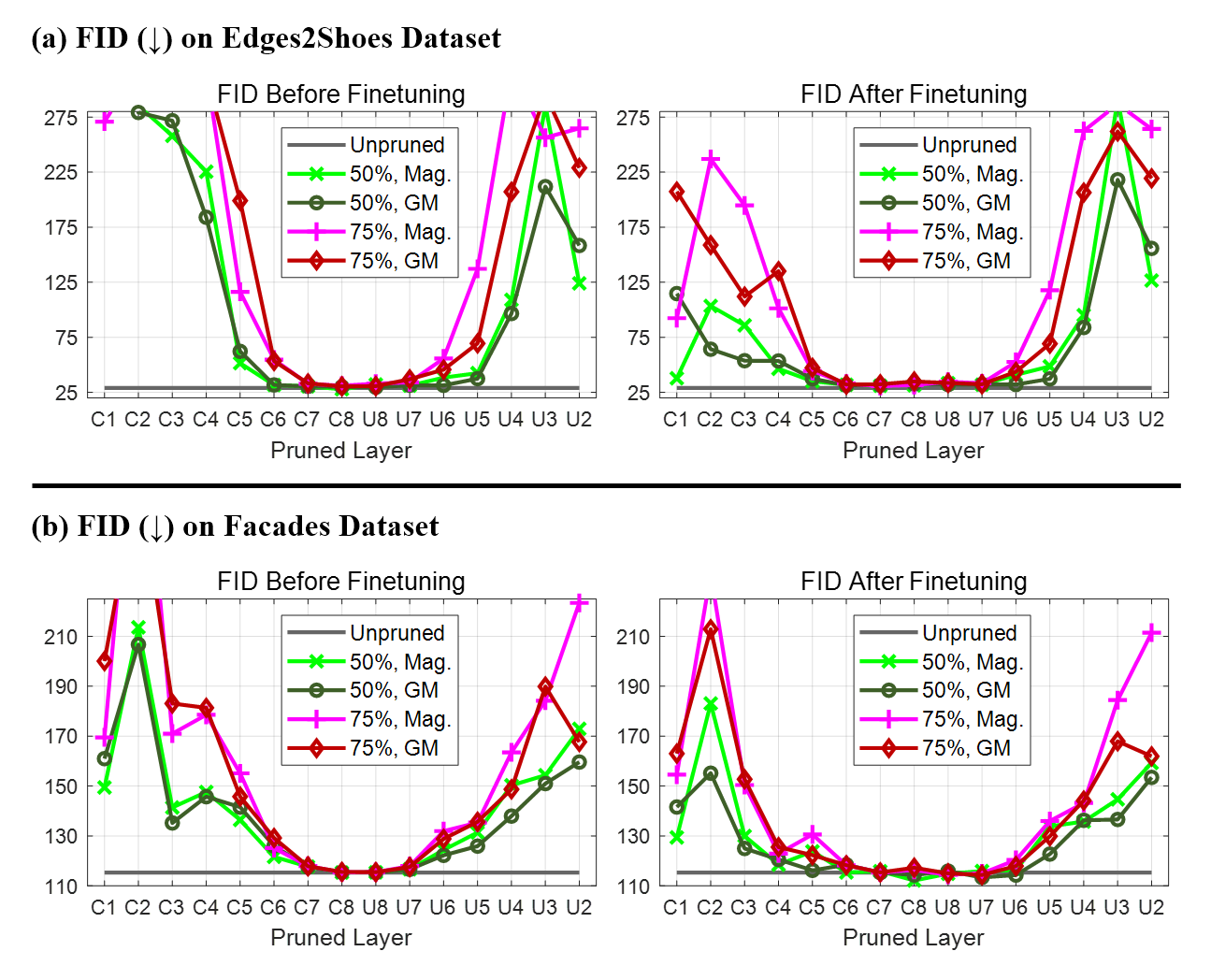
Beyond the importance-based criterion using weight magnitude, we investigate the redundancy-based criterion using geometric median (He et al., 2019). Figure 7 compares the two criteria in the sensitivity analysis using the large generator of Pix2Pix. A consistent trend is observed regardless of the pruning criteria: the innermost layers in the U-Net contain a large number of unnecessary filters and are highly prunable. From this observation, we can understand the network behavior that mainly utilizes the outer layers and their skip connections for fulfilling the generation task.

6 Conclusion

We demonstrate high prunability of the inner layers in U-Net generators and present filter- and layer-level structured pruning methods that exploit the layer characteristics. We believe that the insights from our study can help understanding and improving the generator architectures for GANs. Combining our approach with knowledge distillation to boost the performance and with quantization for further compression would be a promising future direction.

References

Afouras et al. (2018) Afouras, T., Chung, J. S., and Zisserman, A. Lrs3-ted: a large-scale dataset for visual speech recognition. arXiv preprint arXiv:1809.00496, 2018.
Andreev et al. (2021) Andreev, P., Fritzler, A., and Vetrov, D. Quantization of generative adversarial networks for efficient inference: a methodological study. arXiv preprint arXiv:2108.13996, 2021.
Chen et al. (2021a) Chen, T., Cheng, Y., Gan, Z., Liu, J., and Wang, Z. Data-efficient gan training beyond (just) augmentations: A lottery ticket perspective. In NeurIPS, 2021a.
Chen et al. (2021b) Chen, X., Zhang, Z., Sui, Y., and Chen, T. Gans can play lottery tickets too. In ICLR, 2021b.
Chung & Zisserman (2016) Chung, J. S. and Zisserman, A. Out of time: automated lip sync in the wild. In ACCV, 2016.
Frankle & Carbin (2019) Frankle, J. and Carbin, M. The lottery ticket hypothesis: Finding sparse, trainable neural networks. In ICLR, 2019.
Fu et al. (2020) Fu, Y., Chen, W., Wang, H., Li, H., Lin, Y., and Wang, Z. Autogan-distiller: Searching to compress generative adversarial networks. In ICML, 2020.
Gale et al. (2019) Gale, T., Elsen, E., and Hooker, S. The state of sparsity in deep neural networks. In ICML Workshop, 2019.
Gao et al. (2020) Gao, C., Chen, Y., Liu, S., Tan, Z., and Yan, S. Adversarialnas: Adversarial neural architecture search for gans. In CVPR, 2020.
Ghosh et al. (2019) Ghosh, S., Srinivasa, S. K., Amon, P., Hutter, A., and Kaup, A. Deep network pruning for object detection. In ICIP, 2019.
Gong et al. (2019) Gong, X., Chang, S., Jiang, Y., and Wang, Z. Autogan: Neural architecture search for generative adversarial networks. In ICCV, 2019.
Goodfellow et al. (2014) Goodfellow, I., Pouget-Abadie, J., Mirza, M., Xu, B., Warde-Farley, D., Ozair, S., Courville, A., and Bengio, Y. Generative adversarial nets. In NeurIPS, 2014.
Hanson & Pratt (1988) Hanson, S. and Pratt, L. Comparing biases for minimal network construction with back-propagation. In NeurIPS, 1988.
He et al. (2019) He, Y., Liu, P., Wang, Z., Hu, Z., and Yang, Y. Filter pruning via geometric median for deep convolutional neural networks acceleration. In CVPR, 2019.
Heusel et al. (2017) Heusel, M., Ramsauer, H., Unterthiner, T., Nessler, B., and Hochreiter, S. Gans trained by a two time-scale update rule converge to a local nash equilibrium. In NeurIPS, 2017.
Hinton et al. (2014) Hinton, G., Vinyals, O., and Dean, J. Distilling the knowledge in a neural network. In NeurIPS Workshop, 2014.
Hou et al. (2021) Hou, L., Yuan, Z., Huang, L., Shen, H., Cheng, X., and Wang, C. Slimmable generative adversarial networks. In AAAI, 2021.
Isola et al. (2017) Isola, P., Zhu, J.-Y., Zhou, T., and Efros, A. A. Image-to-image translation with conditional adversarial networks. In CVPR, 2017.
Jin et al. (2021) Jin, Q., Ren, J., Woodford, O. J., Wang, J., Yuan, G., Wang, Y., and Tulyakov, S. Teachers do more than teach: Compressing image-to-image models. In CVPR, 2021.
Kynkäänniemi et al. (2019) Kynkäänniemi, T., Karras, T., Laine, S., Lehtinen, J., and Aila, T. Improved precision and recall metric for assessing generative models. In NeurIPS, 2019.
LeCun et al. (1989) LeCun, Y., Denker, J., and Solla, S. Optimal brain damage. In NeurIPS, 1989.
Lee et al. (2021) Lee, J., Park, S., Mo, S., Ahn, S., and Shin, J. Layer-adaptive sparsity for the magnitude-based pruning. In ICLR, 2021.
Li et al. (2017) Li, H., Kadav, A., Durdanovic, I., Samet, H., and Graf, H. P. Pruning filters for efficient convnets. In ICLR, 2017.
Li et al. (2020) Li, M., Lin, J., Ding, Y., Liu, Z., Zhu, J.-Y., and Han, S. Gan compression: Efficient architectures for interactive conditional gans. In CVPR, 2020.
Li et al. (2021) Li, S., Wu, J., Xiao, X., Chao, F., Mao, X., and Ji, R. Revisiting discriminator in gan compression: A generator-discriminator cooperative compression scheme. In NeurIPS, 2021.
Li et al. (2022) Li, S., Lin, M., Wang, Y., Fei, C., Shao, L., and Ji, R. Learning efficient gans for image translation via differentiable masks and co-attention distillation. IEEE Trans. Multimedia, 2022.
Lin et al. (2019) Lin, S., Ji, R., Li, Y., Deng, C., and Li, X. Toward compact convnets via structure-sparsity regularized filter pruning. IEEE Trans. Neural Netw. Learn. Syst., 31(2):574–588, 2019.
Liu et al. (2021) Liu, Y., Shu, Z., Li, Y., Lin, Z., Perazzi, F., and Kung, S.-Y. Content-aware gan compression. In CVPR, 2021.
Mordido et al. (2021) Mordido, G., Yang, H., and Meinel, C. Evaluating post-training compression in gans using locality-sensitive hashing. arXiv preprint arXiv:2103.11912, 2021.
Naeem et al. (2020) Naeem, M. F., Oh, S. J., Uh, Y., Choi, Y., and Yoo, J. Reliable fidelity and diversity metrics for generative models. In ICML, 2020.
Ning et al. (2020) Ning, X., Zhao, T., Li, W., Lei, P., Wang, Y., and Yang, H. Dsa: More efficient budgeted pruning via differentiable sparsity allocation. In ECCV, 2020.
Prajwal et al. (2020) Prajwal, K., Mukhopadhyay, R., Namboodiri, V. P., and Jawahar, C. A lip sync expert is all you need for speech to lip generation in the wild. In ACM MM, 2020.
Romero et al. (2015) Romero, A., Ballas, N., Kahou, S. E., Chassang, A., Gatta, C., and Bengio, Y. Fitnets: Hints for thin deep nets. In ICLR, 2015.
Ronneberger et al. (2015) Ronneberger, O., Fischer, P., and Brox, T. U-net: Convolutional networks for biomedical image segmentation. In MICCAI, 2015.
Shih et al. (2019) Shih, K.-H., Chiu, C.-T., and Pu, Y.-Y. Real-time object detection via pruning and a concatenated multi-feature assisted region proposal network. In ICASSP, 2019.
Shu et al. (2019) Shu, H., Wang, Y., Jia, X., Han, K., Chen, H., Xu, C., Tian, Q., and Xu, C. Co-evolutionary compression for unpaired image translation. In ICCV, 2019.
Sze et al. (2017) Sze, V., Chen, Y.-H., Yang, T.-J., and Emer, J. S. Efficient processing of deep neural networks: A tutorial and survey. Proc. IEEE, 105(12):2295–2329, 2017.
Tousi et al. (2021) Tousi, A., Jeong, H., Han, J., Choi, H., and Choi, J. Automatic correction of internal units in generative neural networks. In CVPR, 2021.
Tyleček & Šára (2013) Tyleček, R. and Šára, R. Spatial pattern templates for recognition of objects with regular structure. In GCPR, 2013.
Wan et al. (2020) Wan, D., Shen, F., Liu, L., Zhu, F., Huang, L., Yu, M., Shen, H. T., and Shao, L. Deep quantization generative networks. Pattern Recognition, 105:107338, 2020.
Wang et al. (2020) Wang, H., Gui, S., Yang, H., Liu, J., and Wang, Z. Gan slimming: All-in-one gan compression by a unified optimization framework. In ECCV, 2020.
Wang et al. (2019) Wang, P., Wang, D., Ji, Y., Xie, X., Song, H., Liu, X., Lyu, Y., and Xie, Y. Qgan: Quantized generative adversarial networks. arXiv preprint arXiv:1901.08263, 2019.
Wen et al. (2016) Wen, W., Wu, C., Wang, Y., Chen, Y., and Li, H. Learning structured sparsity in deep neural networks. In NeurIPS, 2016.
Xie et al. (2020) Xie, Z., Zhu, L., Zhao, L., Tao, B., Liu, L., and Tao, W. Localization-aware channel pruning for object detection. Neurocomputing, 403:400–408, 2020.
Yang et al. (2020) Yang, H., Zhang, R., Guo, X., Liu, W., Zuo, W., and Luo, P. Towards photo-realistic virtual try-on by adaptively generating-preserving image content. In CVPR, 2020.
Yeom et al. (2021) Yeom, S.-K., Seegerer, P., Lapuschkin, S., Binder, A., Wiedemann, S., Müller, K.-R., and Samek, W. Pruning by explaining: A novel criterion for deep neural network pruning. Pattern Recognition, 115:107899, 2021.
Yu & Grauman (2014) Yu, A. and Grauman, K. Fine-grained visual comparisons with local learning. In CVPR, 2014.
Yu & Pool (2020) Yu, C. and Pool, J. Self-supervised generative adversarial compression. In NeurIPS, 2020.

Appendix

Appendix A Generator Architectures

A.1 Pix2Pix

Pix2Pix (Isola et al., 2017) is a popular conditional GAN for image-to-image translation tasks. Figure 2(a) shows its U-Net generator. The encoder consists of convolutional layers that progressively downsample the input to capture the global image context, and the decoder consists of transposed convolutional layers that progressively upsample the bottleneck features to produce the output. The spatial size of the bottleneck feature maps becomes 1×1. Skip connections are used to deliver the encoded feature maps directly to the decoder, improving the generation quality. We test our method for the original large-capacity generator ( $\textrm{nF}=64$ ) and a smaller one ( $\textrm{nF}=32$ ).

A.2 Wav2Lip

Wav2Lip (Prajwal et al., 2020) is a GAN designed for speech-driven talking face generation. Unlike the single-path encoder of Pix2Pix, its generator contains a double-path encoder, as shown in Figure 2(b). The audio encoder takes a speech segment as input, and the face encoder takes a reference frame concatenated with a pose-prior frame. Both encoders map their inputs to the 1×1 embedding vectors, which are concatenated at the bottleneck. The decoder produces a face image of the reference identity that matches the given speech with proper lip synchronization. Skip connections are added between the face encoder and the decoder.

We build an efficient yet effective generator by halving the number of filters (i.e., ( $\mathrm{nVF}$ , $\mathrm{nAF}$ , $\mathrm{nDF}$ ) changes from (16, 32, 32) to (8, 16, 16)) and removing all the residual blocks from the original model. This compressed generator is trained from scratch and becomes the target of pruning.

Appendix B Comparison of Retraining Scenarios

We compare the following settings for retraining pruned generators with adversarial learning. For brevity, $G$ and $D$ denote the generator and discriminator, respectively.

•

(i) Motivated by Frankle & Carbin (2019), we re-initialize the pruned $G$ with random weights. Considering the balance between $G$ and $D$ , we also re-initialize $D$ and jointly train $G$ and $D$ from scratch.
•

(ii) We use the pruned $G$ with its pretrained weights as initialization. The pretrained $D$ is freezed (not updated) but provides learning signals for retraining $G$ .
•

(iii) This setting is the same as ‘(ii)’ except that the pretrained $D$ is jointly trained with the pruned $G$ . We use it throughout this work.

Table 4 summarizes the results of the three scenarios for layer-level pruning. Regardless of the type of removed innermost layers, ‘(ii)’ performs worse than ‘(i)’ and ‘(iii)’, indicating that the pruned generators cannot receive meaningful gradients from the freezed discriminators.⁵⁵5A possible reason why ‘(ii)’ fails is as follows: a well-pretrained $D$ cannot distinguish real and generated images and produces the output probability of 0.5 for both image types. In ‘(ii)’, $G$ being retrained generates the images whose probability becomes assigned as 1 by $D$ . This causes a distribution shift of $D$ ’s outputs and may not yield helpful gradients for retraining $G$ . In addition, ‘(ii)’ does not match the concept of adversarial learning where the balance between the generator and discriminator must be well kept.

In our experiments, ‘(iii)’ consistently outperforms ‘(i)’ for different datasets and pruned architectures, suggesting that finetuning pretrained discriminators jointly with pruned generators is beneficial.

FID (↓) on Edges2Shoes Dataset Layer Removal # Removed Innermost Layers 2 4 6 Bottleneck Size 2×2 4×4 8×8 Retraining Scenario (i) Rand. Init. + Train $D$ 31.8 32.2 63.7 (ii) Pretrained Init. + Freeze $D$ 47.8 71.5 108.7 (iii) Pretrained Init. + Train $D$ 28.3 29.7 38.7 FID (↓) on Facades Dataset Layer Removal # Removed Innermost Layers 2 4 6 Bottleneck Size 2×2 4×4 8×8 Retraining Scenario (i) Rand. Init. + Train $D$ 115.2 112.2 113.5 (ii) Pretrained Init. + Freeze $D$ 158.5 159.0 181.8 (iii) Pretrained Init. + Train $D$ 107.9 108.7 107.8

Table 4: Comparison of different settings for retraining layer-pruned generators.

Appendix C Implementation Details

We use the following hyperparameters in the experiments:

•
Common setup for Pix2Pix models
- –
  
  Initial learning rate (LR): 0.0002
- –
  
  GAN loss: Hinge
- –
  
  Optimizer: Adam with ( $\beta 1$ , $\beta 2$ )=(0.5, 0.999)

•
Pix2Pix on the Edge2Shoes dataset
- –
  
  Batch size: 32
- –
  
  # (Pretraining, Retraining) epochs: (200, 15)
- –
  
  LR schedule: Linear decay to zero after the (100, 10)-th epoch for (pretraining, retraining)

•
Pix2Pix on the Facades dataset
- –
  
  Batch size: 1
- –
  
  # (Pretraining, Retraining) epochs: (300, 20)
- –
  
  LR schedule: Linear decay to zero after the (200, 15)-th epoch for (pretraining, retraining)

•
Wav2Lip on the LRS3 dataset
- –
  
  Initial LR: 0.0001
- –
  
  GAN loss: Standard
- –
  
  Optimizer: Adam with ( $\beta 1$ , $\beta 2$ )=(0.5, 0.999)
- –
  
  Batch size: 16
- –
  
  # (Pretraining, Retraining) epochs: (270, 50)
- –
  
  LR schedule: N/A