Cooperative Retriever and Ranker in Deep Recommenders

Abstract.

Deep recommender systems (DRS) are intensively applied in modern web services. To deal with the massive web contents, DRS employs a two-stage workflow: retrieval and ranking, to generate its recommendation results. The retriever aims to select a small set of relevant candidates from the entire items with high efficiency; while the ranker, usually more precise but time-consuming, is supposed to further refine the best items from the retrieved candidates. Traditionally, the two components are trained either independently or within a simple cascading pipeline, which is prone to poor collaboration effect. Though some latest works suggested to train retriever and ranker jointly, there still exist many severe limitations: item distribution shift between training and inference, false negative, and misalignment of ranking order. As such, it remains to explore effective collaborations between retriever and ranker.

In this work, we present a novel framework for the joint training of retriever and ranker, named CoRR (Cooperative Retriever and Ranker). With CoRR, the retriever is improved by deriving high-quality training signals from the ranker, while the ranker is improved by learning to discriminate hard negatives sampled by the retriever. We introduce two critical techniques. Firstly, we develop an adaptive and scalable sampler based on the retriever, to generate hard negative samples for the ranker’s training. Compared with the widely-used exact top-k sampling, our method effectively alleviates the issues of false negative and item distribution shift, and thus improves the ranker’s discriminability. Secondly, we propose a novel asymptotic-unbiased estimation of KL divergence, which serves as the objective for knowledge distillation. The new objective can be efficiently optimized with commonly-used optimizers. More importantly, it leads to better alignment of ranking order between retriever and ranker, which helps to improve the retrieval quality. We conduct comprehensive experiments over four large-scale datasets, where CoRR outperforms both conventional DRS and the existing joint training methods with notable advantages. Our code will be open-sourced to facilitate future research.

1. Introduction

Recommender system plays an important role in modern web services, like e-commerce and online advertising, as it largely mitigates the information overload problem by suggesting users with personalized items according to their own interests. Thanks to the remarkable progress of deep learning, deep recommender systems (DRS) become increasingly popular in practice (Covington et al., 2016; Hidasi et al., 2015; Ying et al., 2018; Feng et al., 2022; Lian et al., 2020b; Jin et al., 2020; Wu et al., 2021; Feng et al., 2023). Given the magnificent scale of online items, deep recommender systems call for a two-stage workflow: retrieval and ranking (Covington et al., 2016). Particularly, the retriever targets on selecting a small set of candidate items under a certain context (e.g., user profile and historical interactions) from the whole items with high efficiency. Typically, the retriever model learns to represent the context and items as dense embeddings, such that user’s preference towards the items can be efficiently estimated based on embedding similarities, like inner product or cosine similarity. In contrast, the ranker is used to refine the most preferred items from the retrieval results. For the sake of best precision, it usually leverages highly expressive yet time-consuming networks, especially those establishing deep interactions between the context and the item (e.g., DIN (Zhou et al., 2018), DIEN (Zhou et al., 2019) and DeepFM (Guo et al., 2017)).

1.1. Existing Problems

Despite the collaborative nature of the retriever and ranker, the typical training workflow of the two models lacks effective cooperation, which severely harms the overall recommendation quality. In many cases, the two models are independently trained and directly applied to the recommender systems (Zhu et al., 2018; Cen et al., 2020; Zhou et al., 2018, 2019; Lian et al., 2020c). At other times, the ranker can be successively trained based on retrieval results (Gallagher et al., 2019; Hron et al., 2021); whereas, the retriever remains independently trained (Covington et al., 2016). Such training workflows are inferior due to the following reasons.

$\bullet$ The independent training of the retriever only leverages the historical user-item interactions, which can be limited in reality. As a result, it may suffer from the sparsity of training data, which severely restricts the retrieval quality. For another thing, the retriever is likely to generate candidate items that are not favored by the ranker; thus, it may harm the downstream performance as well.

$\bullet$ The independently-trained ranker is learned with randomly or heuristically collected training samples. Such training samples can be too easy to be distinguished, making the ranker converge to a limited discriminative capacity. Besides, the item distribution will also be highly differentiated between the training and inference stages; as a result, the ranker may not effectively recognize the high-quality candidates generated by the retriever.

Recent studies on multi-stage ranking models are closely related to the problem of retriever-ranker collaboration; e.g., in (Qin et al., 2022), a two-pass training workflow is proposed. However, the two-pass workflow is still limited from several critical perspectives. In the forward pass, the rankers are trained by the retrieval results at the exact top-k cutoff, which is prone to false-negatives. Besides, when the retrieval cutoffs are changed during the inference stage, the rankers will face highly shifted item distributions from the training stage, which may severely harm their prediction accuracy. In the backward pass, the retrievers are trained to preserve the consistency of absolute ranking scores and to distinguish ranking results from retrieval ones; while for the sake of high-quality retrieval, it is the consistency of relative ranking order that really matters. In all, it remains a challenging problem to explore more effective collaboration mechanisms between the retriever and ranker.

1.2. Our Solution

In this work, we propose a novel framework for the cooperative training of the retriever and ranker, a.k.a. CoRR (Cooperative Retriever and Ranker). In our framework, the retriever and ranker are simultaneously trained within a unified workflow, where both models can be mutually reinforced.

$\bullet$ Training of retriever. On one hand, the retriever is learned from both user-item interactions via sampled softmax and the ranker’s predictions via knowledge distillation (Hinton et al., 2015). In a specific context, a few items are sampled firstly. Then, the ranker is required to predict the fine-grained preferences towards the sampled items. Rather than preserving the absolute preference scores, the retriever is required to generate the same ranking order for the sampled items as the ranker. To realize this goal, the KL-divergence is minimized for the softmax-normalized predictions between the retriever and ranker (Hinton et al., 2015). In this case, user’s preferred items, whether interacted or not, will probably get highly-rated by the ranker, while real non-interested items get lower-rated (thanks to the highly-precise ranker). As a result, such items will virtually become labeled samples, which substantially augment the training data.

$\bullet$ Training of ranker. The ranker is trained by sampled softmax (Bengio and Senécal, 2008) on top of the hard negative items sampled by the retriever. Particularly, instead of working with the “easy negatives” which are randomly or heuristically sampled from the whole item set (Rendle et al., 2009; Zhou et al., 2018; Guo et al., 2017), the ranker is iteratively trained to discriminate the true positive from the increasingly harder negatives as the retriever improves. Therefore, it prevents the ranker from converging too early to a limited discriminative capability. Besides, unlike the widely-used exact top-k sampling, we collect informative negative samples from the entire itemset based on the retriever; by doing so, it alleviates the false negative issue and closes the gap between the training and inference stages.

It’s worth noting that the realization of the above training framework is non-trivial. Particularly, both retriever and ranker need to learn from the sampled items; however, the sampling operation on the retriever can be inefficient and biased. To overcome such challenges, a couple of technical designs are introduced. Firstly, knowing that the directly sampling from retriever can be extremely time-consuming when dealing with a large itemset, we develop a scalable and adaptive sampling strategy, where the items favored by the retriever can be efficiently sampled in sublinear time with item size. Secondly, the direct knowledge distillation over the sampled items is biased and prone to inferior performances. To mitigate this problem, we propose a novel asymptotic-unbiased estimation of KL divergence for compensating the bias induced by item sampling. On top of this operation, the ranking order of items can be better aligned between the ranker and retriever.

We conduct comprehensive experimental studies over four benchmark datasets. According to the experiment results, the overall recommendation quality can be substantially improved by CoRR in comparison with the existing training methods. More detailed analysis further verifies CoRR’s standalone effectiveness to both the retriever and the ranker, and its effectiveness as a model-agnostic training framework. The contributions of our work are summarized with the following points.

• We present a novel training framework for deep recommender systems, where the retriever and ranker can be mutually reinforced for the effective cooperation.

• Two critical techniques are introduced for the optimized conduct of CoRR: 1) the scalable and adaptive sampling strategy, which enables the efficient sampling from the retriever; 2) the asymptotic-unbiased estimation of KL divergence, as the objective of knowledge distillation, which better aligns the ranking order of items between the ranker and retriever, and contributes to the retrieval of high-quality items.

• We perform comprehensive experimental studies on four benchmark datasets, whose results verify CoRR’s advantage against the existing training algorithms, and its standalone effectiveness to the retriever and ranker.

2. Related Work

This paper studied the cooperation between the ranker and retriever in deep recommender systems, to improve the recommendation quality of multi-stage systems. We first review closely related cascade ranking techniques, and then present negative sampling and knowledge distillation.

2.1. Cascade Ranking

Prior work on multi-stage cascade ranking usually assigned different rankers to each stage to achieve the desired trade-off collectively between efficiency and effectiveness (Wang et al., 2011). They are different from each other in modeling the cost of each ranker (Chen et al., 2017; Xu et al., 2013, 2014). Recent work turned to directly optimizing cascade ranking models as a whole by gradient descent (Gallagher et al., 2019) or identifying some bad cases with cascade ranking models to augment the training data (Fan et al., 2019). Observing these cascading ranking systems do not consider the cooperation between rankers, the work (Qin et al., 2022) suggested to optimize them jointly by letting cascade rankers provide supervised signals for each other in the cascading systems. However, the work is still limited from several critical perspectives, as aforementioned. This work aims to explore a better collaboration mechanism between cascade rankers.

2.2. Negative Sampling in RecSys

Many methods sample negative items from static distributions, such as uniform distribution (Rendle et al., 2009; He et al., 2017) and popularity-based distribution (Rendle and Freudenthaler, 2014). To adapt to recommendation models, many advanced sampling methods have been proposed (Rendle and Freudenthaler, 2014; Hsieh et al., 2017; Weston et al., 2010; Zhang et al., 2013; Sun et al., 2019a; Blanc and Rendle, 2018; Chen et al., 2021; Lian et al., 2020a). For example, AOBPR (Rendle and Freudenthaler, 2014) transforms adaptive sampling into searching the item at a randomly-drawn rank. CML (Hsieh et al., 2017) and WARP (Weston et al., 2010) draw negative samples for each positive by first drawing candidate items from uniform distribution and then selecting more highly-scored items than positive minus one as negative. Dynamic negative sampling (DNS) (Zhang et al., 2013) picks a set of negative samples from the uniform distribution and then chooses the most highly-scored item as negative. Self-adversarial negative sampling (Sun et al., 2019a) draws negative samples from the uniform distribution but weights them with softmax-normalized scores. Kernel-based sampling (Blanc and Rendle, 2018) picks samples proportionally to a quadratic kernel in a divide and conquer way. Locality Sensitive Hashing (LSH) over randomly perturbed databases enables sublinear time sampling and LSH itself can generate correlated and unnormalized samples (Spring and Shrivastava, 2017). Quantization-based sampling (Chen et al., 2021) decomposes the softmax-normalized probability via product quantization into the product of probabilities over clusters, such that sampling an item is in sublinear time.

2.3. Knowledge Distillation in RecSys

KD (Hinton et al., 2015) provides a powerful model-agnostic framework for compressing a teacher model into a student model, by learning to imitate predictions from the teacher. Therefore, KD has been applied in RecSys for compressing deep recommenders. A pioneering work is Ranking Distillation (RD) (Tang and Wang, 2018b), where the top-$k$ recommendation from the teacher model is considered as position-weighted pseudo positive. The subsequent distillation methods improve the use of the top-$k$ recommendations, such as drawing a sample from the top-k items via ranking-based distribution (Lee et al., 2019), its mixture with uniform distribution (Kang et al., 2020) and rank discrepancy-aware distribution (Kweon et al., 2021). In addition to teacher’s prediction, the latent knowledge in the teacher can be distilled into the student via hint regression (Kang et al., 2020) and topology distillation (Kang et al., 2021).

3. Cooperative Retriever and Ranker

In this section, we first overview the training of the CoRR on a training dataset $\mathcal{D}=\{(c,k)\}$, which consists of pairs of a context $c$ and a positive item $k$. The context indicates all information except items, such as user, interaction history, time and location. Following that, we elaborate on how to train the ranker with the retriever based on hard negative sampling and how to train the retriever with the ranker based on knowledge distillation.

3.1. Overview

For the sake of scalable recommendation, deep recommender relies on the collaboration of two models: the retrieval model (retriever) and the ranking model (ranker). The retriever targets on selecting a small set of potentially positive items from the whole items with high efficiency. Typically, the retriever is represented by $M_{\theta}(i,c)=\text{sim}\big{(}E_{\theta_{1}}(i),E_{\theta_{2}}(c)\big{)}$, i.e., the similarity (e.g. Euclidean distance, inner product and cosine similarity) between item embedding $E_{\theta_{1}}(i)$ and context embedding $E_{\theta_{2}}(c)$. Therefore, we can use off-the-shelf ANNs, such as FAISS (Johnson et al., 2017) and SCANN (Guo et al., 2020), for retrieving the most similar items as candidates in sublinear time. The ranker aims to identify the best items from the retrieval results with high precision, and is usually represented by expressive yet time-consuming networks $R_{\phi}(i,c)$ directly taking an item $i$ and a context $c$ as inputs.

Due to time-consuming computation in the ranker, in most cases, traditional training methods learn to discriminate positive from randomly picked negatives. In spite of simplicity, the ranker is trained independently to the retriever. In some cases, the ranker is trained by discriminating positives from the top-k retrieval results from the retriever. In spite of establishing a connection with the retriever, the ranker easily suffers from the false negative issue, since potential positives are definitely included in the top-k retrieval results. Moreover, these negatives may introduce a large bias to gradient, such that the optimization may converge slowly and even be easily stuck into a local optimum. To this end, we suggest to optimize the ranker w.r.t the sampled log-softmax (Bengio and Senécal, 2008), an asymptotic-unbiased estimation of log-softmax based on importance sampling. The sampled log-softmax relies on randomly-drawn samples from a proposal distribution. To connect the ranker with the retriever, we propose to sample negatives from the retriever based on an adaptive and scalable strategy.

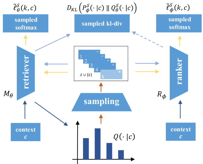
Figure 1. The framework of CoRR. The context $c$ indicates all information except items. $Q(\cdot|c)$ indicates the proposal distribution given context $c$. The dotted line means the gradient is stopped.

[The framework of CoRR.]Fully described in the text in Section 3.1.

In addition to supervision from data, the training of the retriever can also be guided by the ranker based on knowledge distillation since the ranker is assumed more precise at ranking items. Regarding supervision from recommendation data, the sampled log-softmax objective is also exploited for optimizing the retriever with the same proposal in the ranker optimization. Regarding knowledge distillation from the ranker, most prior methods distill knowledge in top-k results from the ranker (Tang and Wang, 2018b; Lee et al., 2019; Kang et al., 2020), but the top-k ranking results are time-consuming for the ranker. In this paper, we distill the ranking order information from the ranker’s predictions, by directly aligning softmax-normalized predictions between the ranker and retriever based on the KL divergence. To reduce the time cost of optimization, we propose an asymptotic-unbiased estimation for the KL divergence, named sampled KL divergence.

The retriever and ranker are simultaneously trained with a unified workflow, where both models can be mutually reinforced. As the training progresses, the ranker becomes increasingly precise, which in return provides more informative supervision signals for the retriever; meanwhile, as the retriever improves, negative samples will become increasingly harder, which contributes to a higher discriminative capability of the ranker. The overall framework is illustrated in Figure 1. The overall procedure can be referred to in Algorithm 1.

3.2. Training Ranker with Retriever

3.2.1. Loss Function

In this paper, we optimize the ranker w.r.t sampled log-softmax, which is an asymptotic-unbiased estimation of log-softmax. The use of log-softmax is motivated by its close relationship with the logarithm of both Mean Reciprocal Rank (MRR) and Normalized Discounted Cumulative Gain (NDCG) (Bruch et al., 2019) as well as the excellent recommendation performance (Liang et al., 2018). Assuming the positive item is $k$ at a context $c$, the log-softmax objective w.r.t $k$ is formulated as follows:

$$\ell(k,c) =R_{\phi}(k,c)-\log\Big{(}\sum_{i}\exp\big{(}R_{\phi}(i,c)\big{)}\Big{)}$$

$$=-\log\Big{(}\sum_{i}\exp\big{(}R_{\phi}(i,c)-R_{\phi}(k,c)\big{)}\Big{)}$$

$$\leq-\log\Big{(}\sum_{i}\mathbb{I}_{\geq 0}\big{(}R_{\phi}(i,c)-R_{\phi}(k,c)\big{)}\Big{)}$$

$$=\log\Big{(}\frac{1}{\text{rank}_{R}(k,c)}\Big{)}=\log\text{MRR}$$

where the inequality holds due to $\exp(\cdot)\geq\mathbb{I}_{\geq 0}(\cdot)$.

Input: Training Data $\mathcal{D}$

Output: Retriever $M_{\theta}$ and Ranker $R_{\phi}$

1 repeat

2       foreach $(c,k)\in\mathcal{D}$ do

3             $\mathcal{S}\leftarrow$ Draw $n$ samples according to ${Q}(\cdot|c)$;

4             Update $M_{\theta}$ w.r.t. $\tilde{\ell}_{\theta}^{\mathcal{S}}(k,c)+D_{KL}(P_{\phi}^{\mathcal{S}}(\cdot|c)\parallel{P}_{\theta}^{\mathcal{S}}(\cdot|c))$;

5             Update $R_{\phi}$ w.r.t. $\tilde{\ell}_{\phi}^{\mathcal{S}}(k,c)$;

6            

7      

8until Convergence or reaching maxepoch;

Algorithm 1 Cooperative Retriever and Ranker

However, it is computationally challenging to optimize the log-softmax, since the gradient computation scales linearly with the number of items, i.e.,

$$\nabla\ell_{\phi}(k,c)=\nabla R_{\phi}(k,c)-\mathbb{E}_{i\sim P_{\phi}(\cdot|c)}[\nabla R_{\phi}(i,c)]$$

where $P_{\phi}(\cdot|c)$ represents categorical probability distribution over the whole items $\mathcal{I}$ with the parameter $\text{softmax}(R_{\phi}(\cdot,c))$, i.e., $P_{\phi}(j|c)=\frac{\exp(R_{\phi}(j,c)}{\sum_{i\in\mathcal{I}}\exp(R_{\phi}(i,c))}$. To improve the efficiency, importance sampling was used for approximation by drawing $L$ samples $\mathcal{S}=\{o_{1},\cdots,o_{L}\}$ from the proposal distribution ${Q}(\cdot|c)$. That is,

$$\nabla\ell_{\phi}(k,c)\approx\nabla R_{\phi}(k,c)-\sum_{i\in\mathcal{S}\cup\{k\}}w(i,c)\nabla R_{\phi}(i,c)$$

where $w(i,c)=\frac{\exp\big{(}R_{\phi}(i,c)-\log\tilde{Q}(i|c)\big{)}}{\sum_{j\in\mathcal{S}\cup\{k\}}\exp\big{(}R_{\phi}(j,c)-\log\tilde{Q}(j|c)\big{)}}$. It is easy to verify that this gradient can be derived from the following sampled log-softmax.

(1) $$\tilde{\ell}_{\phi}^{\mathcal{S}}(k,c)=\log\frac{\exp\big{(}R_{\phi}(k,c)-\log\tilde{Q}(k|c)\big{)}}{\sum_{i\in\mathcal{S}\cup\{k\}}\exp\big{(}R_{\phi}(i,c)-\log\tilde{Q}(i|c)\big{)}}$$

where $\tilde{Q}(\cdot|c)$ is the unnormalized ${Q}(\cdot|c)$. Note that both positive item $k$ and sampled itemset $\mathcal{S}$ are used in these formulations. This is because it is necessary to guarantee negativeness of the sampled log-softmax like log-softmax. To connect the ranker with the retriever, we propose to construct the proposal distribution from the retriever $M_{\theta}$ in this paper. In the next part, we will elaborate on how to efficiently sample items based on the retriever.

3.2.2. Sampling from the Retriever

Prior work considered the top-k retrieval results as negative, they suffer from the false negative issues since the top-k results include both hard negatives and potential positives. In this paper, we propose to construct the proposal distribution from the retriever $M_{\theta}$, i.e., $Q(i|c)=P_{\theta}(i|c)=\frac{\exp\big{(}M_{\theta}(i,c)/T\big{)}}{\sum_{j\in\mathcal{I}}\exp\big{(}M_{\theta}(j,c)/T\big{)}}$, where the coefficient $T$ controls the balance between hardness and randomness of negative samples. When $T\rightarrow\infty$, sampling approaches completely random; when $T\rightarrow 0$, it becomes fully deterministic, being equivalent to argmax. In this case, the sampled log-softmax can be reformulated as

$$\tilde{\ell}_{\phi}^{\mathcal{S}}(k,c)=\log\frac{\exp\big{(}R_{\phi}(k,c)-M_{\theta}(k,c)/T\big{)}}{\sum_{i\in\mathcal{S}\cup\{k\}}\exp\big{(}R_{\phi}(i,c)-M_{\theta}(i,c)/T\big{)}}.$$

However, it is time-consuming to draw samples from $P_{\theta}(i|c)$ while sampling efficiency is important for training model. In the part, we introduce a scalable and adaptive sampler, which enables to draw samples from $P_{\theta}(i|c)$ in sublinear time. Basically, the sampler first builds a multi-level inverted index on the item embeddings in retrieval model with the inner product similarity and then draws negative samples based on the index. Regarding index building, each item embedding is first evenly split into two subvectors, and in each subspace, items are clustered with the K-means. Each item can then be approximated by concatenation of the corresponding cluster centers. Particularly, item $i$’s embedding $E_{\theta_{1}}(i)\approx\mathbf{w}_{k(i)}^{1}\oplus\mathbf{w}_{k(i)}^{2}$, where $k(i)$ indicates the cluster assignment of the item $i$ while $\mathbf{w}_{k(i)}^{1}$ and $\mathbf{w}_{k(i)}^{2}$ denote cluster centers of the item $i$. Let $\Omega_{k}^{1}$ and $\Omega_{k}^{2}$ be the item set belong to the cluster $k$ in the first and second subspace respectively and split query vector $\mathbf{z}_{c}=E_{\theta_{2}}(c)$ of the context $c$ into two parts, i.e., $\mathbf{z}_{c}=\mathbf{z}^{1}_{c}\oplus\mathbf{z}^{2}_{c}$. Negative sampling can then be decomposed into the following three steps:

• Sampling a cluster $k^{1}$ in the first subspace. The sampling probability of the cluster $k$ is defined as $P(k)=\frac{\psi_{k}\exp(\langle\mathbf{z}^{1}_{c},\mathbf{w}_{k}^{1}\rangle)}{\sum_{k^{\prime}}\psi_{k^{\prime}}\exp(\langle\mathbf{z}^{1}_{c},\mathbf{w}_{k^{\prime}}^{1}\rangle)}$, where $\psi_{k}=\sum_{k^{\prime}}\omega_{k,k^{\prime}}\exp(\langle\mathbf{z}^{2}_{c},\mathbf{w}_{k^{\prime}}^{2}\rangle)$ while $\omega_{k,k^{\prime}}=\lvert\Omega_{k}^{1}\cap\Omega_{k^{\prime}}^{2}\rvert$.

• Sampling a cluster $k^{2}$ in the second subspace conditional on $k^{1}$. The sampling probability of the cluster $k$ is defined as $P(k|k^{1})=\frac{\omega_{k^{1},k}\exp(\langle\mathbf{z}^{2}_{c},\mathbf{w}_{k}^{2}\rangle)}{\sum_{k^{\prime}}\omega_{k^{1},k^{\prime}}\exp(\langle\mathbf{z}^{2}_{c},\mathbf{w}_{k^{\prime}}^{2}\rangle)}$.

• Sampling an item uniformly within the intersection item set $\Omega_{k_{1}}^{1}\cap\Omega_{k_{2}}^{2}$.

Remarks on Sampling Effectiveness: In spite of being decomposed, this sampling procedure actually corresponds to sampling from $\hat{Q}(i|c)=\frac{\exp(\langle\mathbf{z}_{c},\mathbf{w}_{k(i)}^{1}\oplus\mathbf{w}_{k(i)}^{2}\rangle)}{\sum_{j}\exp(\langle\mathbf{z}_{c},\mathbf{w}_{k(j)}^{1}\oplus\mathbf{w}_{k(j)}^{2}\rangle)}$. Thanks to the bounded divergence from above between $\hat{Q}(i|c)$ and $Q(i|c)$, the sampling effectiveness can be guaranteed (Chen et al., 2021), depending on the residual error of clustering. When the residual error is smaller, approximate sampling is more closely to exact sampling.

Remarks on Sampling Efficiency: Since $\omega_{k,k^{\prime}}$ is query independent, it can be precomputed after clustering. The overall time complexity of sampling $T$ items is $\mathcal{O}(Kd+K^{2}+T)$, where $d$ is the embedding dimension and $K$ is the number of clusters in K-means.

3.3. Training Retriever with Ranker

Although the retriever has been used for training the ranker, the gradient from the ranker’s objective should be stopped, since the retriever is only used for providing negative information for the ranker. The training of the retriever $M_{\theta}(i,c)$ is then guided by supervision loss from the recommendation data and a distillation loss from the ranker.

3.3.1. Supervision Loss

Since the retriever concerns about the recall performance of retrieval results, it should optimize the ranking performance. Similar to the ranker, the retriever also exploits the sampled log-softmax for optimization as long as simply replacing $R_{\phi}(i|c)$ with $M_{\theta}(i,c)$. We also use the sampler in Section 3.2.2 as the proposal, since it can greatly reduce the cost of forward inference and back-propagation in the retriever by using a few sampled items. Therefore, the objective function is then represented as

(2) $$\tilde{\ell}_{\theta}^{\mathcal{S}}(k,c)=\log\frac{\exp\big{(}M_{\theta}(k,c)-\log\tilde{Q}(k|c)\big{)}}{\sum_{i\in\mathcal{S}\cup\{k\}}\exp\big{(}M_{\theta}(i,c)-\log\tilde{Q}(i|c)\big{)}}$$

3.3.2. Distillation Loss

The high efficiency of the retriever comes at the cost of limited expressiveness. Knowing that the ranker is more precise, the knowledge distillation may provide substantial weak-supervision signals to alleviate the sparsity of training data. Therefore, in this section, we design the knowledge distillation loss from the ranker. Without concentrating on specific recommenders, we consider not distilling latent knowledge but the predictions from the ranker. To avert the use of the top-k results from the ranker in prior work, we follow the pioneering work of KD (Hinton et al., 2015) to directly match softmax-normalized predictions between the ranker and the retriever via KL divergence, that is,

(3) $$D_{KL}\Big{(}P_{\phi}(\cdot|c)\parallel P_{\theta}(\cdot|c)\Big{)}=\sum_{i\in\mathcal{I}}P_{\phi}(i|c)\log\frac{P_{\phi}(i|c)}{P_{\theta}(i|c)},$$

where $P_{\phi}(\cdot|c)$ and $P_{\theta}(\cdot|c)$ are probabilities induced by the ranker and retriever, respectively. However, it is impracticable to directly compute KL divergence and its gradient, since it scales linearly with the number of items w.r.t each context. To this end, we propose an asymptotic-unbiased estimation for the KL divergence for speeding up forward inference and backward propagation. In particular, first denote by $\mathcal{S}=\{o_{1},o_{2},\cdots,o_{L}\}$ the sample set drawn from the proposal ${Q}(\cdot|c)$ and define ${P}_{\phi}^{\mathcal{S}}(j|c)=\frac{\exp(\tilde{R}_{\phi}(j,c))}{\sum_{i\in\mathcal{S}}\exp(\tilde{R}_{\phi}(i,c))}$ and ${P}_{\theta}^{\mathcal{S}}(j|c)=\frac{\exp(\tilde{M}_{\theta}(j,c))}{\sum_{i\in\mathcal{S}}\exp(\tilde{M}_{\theta}(i,c))}$, where $\tilde{R}_{\phi}(i,c)=R_{\phi}(i,c)-\log\tilde{Q}(i|c)$ and $\tilde{M}_{\theta}(i,c)=M_{\theta}(i,c)-\log\tilde{Q}(i|c)$. $D_{KL}\Big{(}{P}_{\phi}^{\mathcal{S}}(\cdot|c)\parallel{P}_{\theta}^{\mathcal{S}}(\cdot|c)\Big{)}$ is the asymptotic-unbiased estimation for $D_{KL}\Big{(}P_{\phi}(\cdot|c)\parallel P_{\theta}(\cdot|c)\Big{)}$ according to the following theorem.

Theorem 3.1.

$D_{KL}\Big{(}{P}_{\phi}^{\mathcal{S}}(\cdot|c)\parallel{P}_{\theta}^{\mathcal{S}}(\cdot|c)\Big{)}$ converges to $D_{KL}\Big{(}P_{\phi}(\cdot|c)\parallel P_{\theta}(\cdot|c)\Big{)}$ with probability 1 when $L=\lvert\mathcal{S}\rvert\rightarrow\infty$.

When used for learning the retriever, the sampled KL divergence is based on the sampler in Section 3.2.2. Below we discuss some special cases of samplers for further understanding its generality.

3.3.3. Special Cases

In this part, we investigate two special proposals: ${Q}(\cdot|c)=P_{\theta}(\cdot|c)=\text{softmax}(M_{\theta}(\cdot,c))$ and ${Q}(\cdot|c)$ is uniform.

$\bullet$ ${Q}(\cdot|c)=P_{\theta}(\cdot|c)$: In this case the ranker is optimized by the sampled log-softmax $\tilde{\ell}(k,c)=\log\frac{\exp(\Delta_{k}^{c})}{\sum_{i\in\mathcal{S}}\exp(\Delta_{i}^{c})}$, where $\Delta_{k}^{c}=R_{\phi}(k,c)-M_{\theta}(k,c)$. The distillation loss could be simplified as follows:

Corollary 3.2.

If each sample in $\mathcal{S}$ is drawn according to $P_{\theta}(\cdot|c)$, concatenating $\{\Delta_{i}^{c}|i\in\mathcal{S}\}$ as a vector $\boldsymbol{\Delta}^{c}$ of length $L$, then $D_{KL}(P_{\phi}\parallel P_{\theta})$ can be asymptotic-unbiasedly estimated by $\log L-H({\text{softmax}}(\boldsymbol{\Delta}^{c}))$, where $H(p)$ is the Shannon entropy of categorical distribution parameterized by $p$.

The proof is provided in the appendix. The corollary indicates that when exactly drawing samples from $P_{\theta}(\cdot|c)$, minimizing the KL divergence is equivalent to maximizing the entropy of a categorical distribution. The distribution is parameterized by softmax-normalized prediction differences between the ranker and retriever.

$\bullet$ ${Q}(\cdot|c)$ is uniform: In this case, the ranker is optimized by the sampled log-softmax $\tilde{\ell}(k,c)=\log\frac{\exp(R_{\phi}(k,c))}{\sum_{i\in\mathcal{S}}\exp(R_{\phi}(i,c))}$. And ${P}_{\mathcal{S}}(\cdot|c)$ and ${Q}_{\mathcal{S}}(\cdot|c)$ could be simplified: ${P}_{\phi}^{\mathcal{S}}(j|c)=\frac{\exp(R_{\phi}(j,c))}{\sum_{i\in\mathcal{S}}\exp(R_{\phi}(i,c))}$ and ${P}_{\theta}^{\mathcal{S}}(j|c)=\frac{\exp(M_{\theta}(j,c))}{\sum_{i\in\mathcal{S}}\exp(M_{\theta}(i,c))}$. Minimizing the KL divergence between them is equivalent to matching the ranking order on the randomly sample set $\mathcal{S}$ between the ranker and retriever.

4. Experiments

Experiments are conducted to verify the effectiveness of the proposed CoRR, by answering the following questions:

• Does CoRR outperforms conventional DRS and the existing joint training methods?

• Could the adaptive sampler generate higher-quality negative items than the exact top-k sampling to help training?

• Does the ranking-order preserving distillation loss improve the retriever?

Since CoRR is model-agnostic, to demonstrate the effectiveness of CoRR, we apply the framework for both general recommendation and sequential recommendation in this paper.

4.1. Experimental Settings

4.1.1. Datasets

As shown in Table 1, we evaluate our method on four real-world datasets. The datasets are from different domains and platforms, and they vary significantly in size and sparsity. Gowalla dataset contains users’ check-in data at locations at different times. Taobao dataset is a big industrial dataset collected by Alibaba Group, which contains user behaviors including click, purchase, adding item to shopping cart, and item favoring. We select the largest subset which contains click behaviors. The Amazon dataset is a subset of product reviews for Amazon Electronics. MovieLens dataset is a classic movie rating dataset, in which ratings range from 0.5 to 5. We choose a subset with 10M interactions to conduct experiments. Then we filter out users and items (locations/products/movies) less than 10 interactions for all datasets.

For general recommendation task, the behavior history of each user is splited in to train/valid/test by ratio 0.8/0.1/0.1. For sequential recommendation task, given the behavior history of a user is $(i_{1},i_{2},\cdots,i_{k},\cdots,i_{n})$, the goal is to predict the $(k+1)$-th items using the first $k$ items. In all experiments, we generate the training set with $k=1,2,\cdots,n-3$ for all users, and we predict the next one given the first $n-2$ and $n-1$ items in the valid and test set respectively. Besides, we set the max sequence length to 20 for the user behavior sequence in all datasets.

Table 1. Dataset Statistics.

	#users	#items	#interactions
Amazon	9,280	6,066	158,979
Gowalla	29,859	40,989	1,027,464
MovieLens	66,958	10,682	5,857,041
Taobao	941,853	1101,236	63,721,355

Table 2. Comparisons with baselines($\times 10^{-2}$). $\triangle$,$\blacktriangle$ indicate the improvements of CoRR over the best results of baselines are statistically significant for $p<0.05$, $p<0.001$ based on t test.

Dataset	Metrics	BPR	NCF	LogisticMF	DSSM	Independent	ICC	RankFlow	CoRR
Amazon	Recall@10	$4.86$	$4.51$	$3.74$	$4.55$	$4.97$	$4.88$	$5.06$	$\mathbf{5.76}^{\blacktriangle}$
	NDCG@10	$2.72$	$2.52$	$2.03$	$2.52$	$2.68$	$2.74$	$2.82$	$\mathbf{3.22}^{\blacktriangle}$
	MRR@10	$2.51$	$2.29$	$1.80$	$2.28$	$2.43$	$2.37$	$2.63$	$\mathbf{3.04}^{\blacktriangle}$
Gowalla	Recall@10	$7.78$	$8.33$	$6.70$	$6.30$	$8.24$	$9.08$	$9.35$	$\mathbf{10.52}^{\blacktriangle}$
	NDCG@10	$5.74$	$5.69$	$4.21$	$4.32$	$6.17$	$6.18$	$6.34$	$\mathbf{7.49}^{\blacktriangle}$
	MRR@10	$7.91$	$7.41$	$4.99$	$5.88$	$7.96$	$8.14$	$8.65$	$\mathbf{10.17}^{\blacktriangle}$
MovieLens	Recall@10	$18.23$	$18.63$	$10.79$	$14.83$	$19.54$	$20.22$	$20.72$	$\mathbf{22.44}^{\triangle}$
	NDCG@10	$16.54$	$16.82$	$9.44$	$13.88$	$17.49$	$17.96$	$18.73$	$\mathbf{21.59}^{\blacktriangle}$
	MRR@10	$25.98$	$26.22$	$15.51$	$22.59$	$27.74$	$27.76$	$28.73$	$\mathbf{33.70}^{\blacktriangle}$
TaoBao	Recall@10	$0.87$	$1.87$	$0.51$	$1.66$	$2.16$	$2.19$	$2.63$	$\mathbf{2.79}^{\triangle}$
	NDCG@10	$0.67$	$0.94$	$0.25$	$0.83$	$1.04$	$1.12$	$1.24$	$\mathbf{1.43}^{\triangle}$
	MRR@10	$0.62$	$0.65$	$0.17$	$0.58$	$0.72$	$0.79$	0.88	$\mathbf{1.02}^{\blacktriangle}$
Dataset	Metrics	GRU4Rec	BERT4Rec	Caser	SASRec	Independent	ICC	RankFlow	CoRR
Amazon	Recall@10	$4.98$	$5.18$	$4.74$	$5.18$	$5.26$	$4.34$	$5.33$	$\mathbf{5.84}^{\triangle}$
	NDCG@10	$2.61$	$2.81$	$2.46$	$2.63$	$2.69$	$2.34$	$2.78$	$\mathbf{3.07}^{\triangle}$
	MRR@10	$1.89$	$2.00$	$1.77$	$1.85$	$1.94$	$1.73$	$2.06$	$\mathbf{2.23}^{\triangle}$
Gowalla	Recall@10	$8.43$	$13.61$	$7.88$	$9.29$	$12.50$	$9.28$	$12.68$	$\mathbf{14.46}^{\triangle}$
	NDCG@10	$4.75$	$7.74$	$4.67$	$5.42$	$7.06$	$5.28$	$7.09$	$\mathbf{8.31}^{\triangle}$
	MRR@10	$3.64$	$5.95$	$3.69$	$4.24$	$5.41$	$4.07$	$5.82$	$\mathbf{6.44}^{\triangle}$
MovieLens	Recall@10	$15.54$	$14.67$	$16.78$	$15.02$	$16.89$	$17.27$	$17.59$	$\mathbf{18.46}^{\blacktriangle}$
	NDCG@10	$7.78$	$7.52$	$8.55$	$7.53$	$8.97$	$9.23$	$9.33$	$\mathbf{9.83}^{\triangle}$
	MRR@10	$5.45$	$5.37$	$6.07$	$5.09$	$5.96$	$6.21$	$6.60$	$\mathbf{7.25}^{\blacktriangle}$
Taobao	Recall@10	$0.49$	$0.68$	$0.37$	$0.30$	$0.89$	$0.88$	$0.94$	$\mathbf{1.16}^{\blacktriangle}$
	NDCG@10	$0.42$	$0.61$	$0.30$	$0.26$	$0.76$	$0.73$	0.89	$\mathbf{1.01}^{\blacktriangle}$
	MRR@10	$0.88$	$1.14$	$0.65$	$0.57$	$1.58$	$1.55$	1.96	$\mathbf{2.13}^{\blacktriangle}$

Table 3. Extensive Retriever and Ranker. ($\times 10^{-2}$)

Dataset	Metric	MF+DeepFM			DSSM+DCN			SASRec+DIN			Caser+BST
		Independent	RankFlow	CoRR	Independent	RankFlow	CoRR	Independent	RankFlow	CoRR	Independent	RankFlow	CoRR
Amazon	Recall@10	4.97	5.06	5.76	4.28	4.44	4.72	5.26	5.33	5.84	4.77	4.79	5.03
	NDCG@10	2.68	2.82	3.22	2.36	2.45	2.68	2.69	2.78	3.07	2.57	2.60	2.72
	MRR@10	2.43	2.63	3.04	2.12	2.24	2.45	1.94	2.06	2.23	1.83	1.87	1.98
Gowalla	Recall@10	8.24	9.35	10.52	7.01	8.12	9.69	12.50	12.68	14.46	10.99	10.68	13.90
	NDCG@10	6.17	6.56	7.54	5.17	6.10	6.73	7.06	7.09	8.31	6.03	6.11	8.27
	MRR@10	7.96	8.94	10.26	7.28	7.94	8.97	5.41	5.82	6.44	4.53	4.73	6.55
MovieLens	Recall@10	19.54	20.72	22.44	18.51	20.37	22.94	16.89	17.59	18.46	17.48	16.54	23.16
	NDCG@10	17.49	18.73	22.26	18.01	20.10	22.08	8.97	9.33	9.83	8.84	8.33	12.59
	MRR@10	27.84	28.73	34.07	29.02	31.53	34.24	5.96	6.60	7.25	6.24	6.22	9.39

4.1.2. Metric

Three common top-k metrics are used in evaluation, NDCG (Weimer et al., 2007), Recall (Hu et al., 2008; Wang and Blei, 2011) and MRR. Recall@k represents the proportion of cases when the target item is among the top k items. NDCG@k gives higher weights on higher ranks. MRR@k represents the average of reciprocal ranks of target items. A greater value of these metrics indicates better performance.

4.1.3. Implementation Details

In this paper, MF (Matrix Factorization) (Koren et al., 2009; Rendle et al., 2009) and DeepFM (Guo et al., 2017) are selected as retriever and ranker respectively in general recommendation. In sequential recommendation, we set SASRec (Kang and McAuley, 2018) as the retriever and DIN (Zhou et al., 2018) as the ranker. In prediction, we first retrieve the top-100 items from all items using the retriever and then rank these items by the ranker for final outputs. For an extensive study of model agnostics, other choices for the retriever and ranker are also considered, as shown in Section 4.3. The source code is released in github.

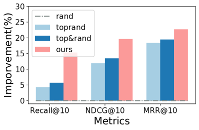
(a) Amazon(base:rand)

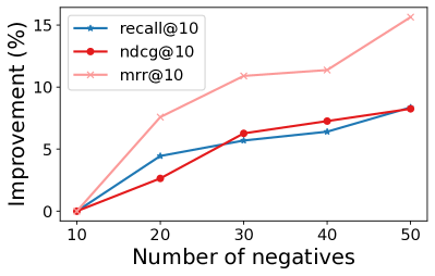
(b) Amazon(base:10 negatives)

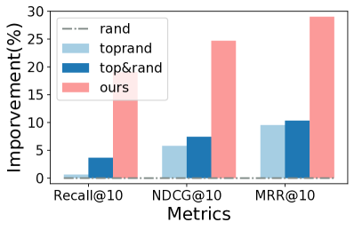
(c) Gowalla(base:rand)

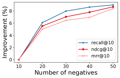
(d) Gowalla(base:10 negatives)

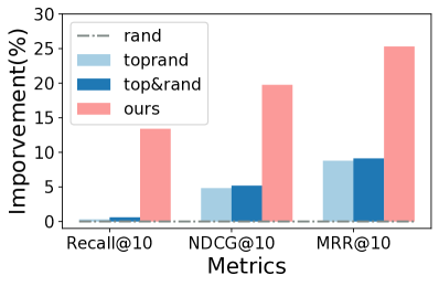
(e) MovieLens(base:rand)

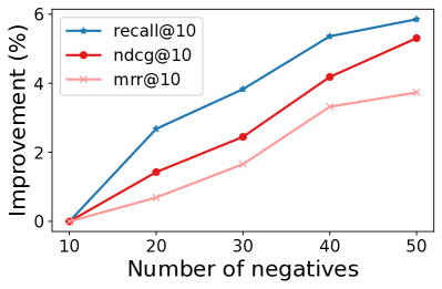
(f) MovieLens(base:10 negatives)

Figure 2. Comparisons among different negative samples generating strategies (left column) and performance w.r.t negative items number (right column). The vertical axis represents the relative improvement to the base (rand for the left column and 10 for the right column).

[Comparisons among different negative samples generating strategies (left column) and performance w.r.t negative items number (right column).]The vertical axis represents the relative improvement to the base (rand for the left column and 10 for the right column). The left column indicates that ours negative samples generating strategy outperforms rand and top-k methods. And the right column indicates that the performance get better as the number of negative items increases.

4.2. Comparison with Baselines

4.2.1. Baselines Methods

We compare the proposed CoRR with four retriever methods and three existing training algorithms (i.e., ICC, RankFlow and Independent). Detailed information of baselines can be referred to in Appendix B.1.

4.2.2. Results

The experimental results on all datasets are reported in Table 2. It shows that CoRR outperforms both conventional DRS and the existing joint training methods with notable advantages. The findings can be summarized as follows:

Finding 1: The Independent training method performs better than all retrievers, though both retriever and ranker are independently trained in The Independent method. In general recommendation, the Independent method outperforms the best retriever by 5.39%, 5.16%, 3.50% overall datasets in terms of Recall@10, NDCG@10 and MRR@10. Similarly in sequential recommendation, the improvements are up to 6.23%, 4.11%, 6.18%. These results indicate that the limited expressiveness of the retriever can be compensated by the ranker and that the retriever and ranker can capture different information in the training data.

Finding 2: All three joint training methods (ICC, RankFlow and CoRR) almost outperform the Independent method. The best of them – CoRR’s average relative improvements in terms of NDCG@10 to the Independent method are 25.62% and 18.57% in two tasks, respectively. This shows that modeling the collaboration between the retriever and ranker remarkably improves the cascading ranking systems. The better collaborative mechanism between them can lead to more improvements.

Finding 3: Among three joint training methods, CoRR performs best in item recommendation. This demonstrates the superiority of the proposed joint training framework. Compared with ICC, in which retriever and ranker are only learned with the training data, CoRR achieves 21.65% and 33.35% average relative improvements in terms of NDCG@10 on all datasets in general recommendation and sequential recommendation, respectively. Compared with RankFlow, in which retriever and ranker are jointly trained and reinforced by each other, CoRR still achieves 15.72% and 11.62% average relative improvements in terms of NDCG@10 on all datasets in these two tasks. The results demonstrate that CoRR’s cooperative training is more effective than RankFlow. More especially, the retriever can improve a lot by knowledge distillation from the ranker in CoRR while the retriever seldom gets improved in RankFlow.

4.3. Extensive Retrievers and Rankers

The proposed CoRR is a model-agnostic training framework, and we consider different combinations of retrievers and rankers to verify the universal effectiveness of CoRR. Experiments are conducted with four different retrievers (i.e., SASRec and Caser for sequential recommendation, MF and DSSM for general recommendation) and four rankers (i.e., DIN and BST for sequential recommendation, DeepFM and DCN for general recommendation) on the three datasets. We take the Independent and RankFlow as the baseline methods for comparison.

Table 3 reports the results of the different combinations of retrievers and rankers. Our proposed CoRR, where the retriever and ranker are cooperatively trained, shows remarkably better performances than the Independent approach, leading to over 15% improvements for any combinations of them. Compared with RankFlow, the relative improvements of CoRR can be up to 10% for each any combinations of retrievers and rankers. This consistently validates the effectiveness of the proposed cooperative training framework and provides evidence of extensive practice for CoRR.

4.4. Comparison of Different Negative Samplers

The hard negative samples play important roles in the training of the rankers, and we compare different baseline strategies with the proposed sampling strategy in Section 3.2.2, named Ours. It is common to regard the top-k retrieval items from the retriever as hard negatives, so we compare our method with several top-k based strategies to verify the effectiveness of our method. They include

• Rand: $n$ items are uniformly sampled from all items.

• TopRand: the top $5n$ items are retrieved by the retriever and then $n$ items are uniformly picked out from the retrieval items.

• Top&Rand: the top $n/2$ items are retrieved by the retriever and $n/2$ items are uniformly sampled from all items.

• Ours: sampling $n$ items from an adaptive and scalable sampler, by approximating softmax probability with subspace clustering.

In the experiments, the number of negative samples $n$ is set to 20. Figure 2(f) reports the experimental results of these negative sampling strategies. It shows that the adaptive sampler can generate higher-quality negative items than the exact top-k sampling method and variants, which remarkably improves model training. The detailed findings are summarized as follows:

Finding 1: Both randomness and hardness are indispensable for sampling high-quality negative items. The superiority of both TopRand and Top&Rand to Rand on all three datasets indicates the importance of hardness in negative sampling since the top-k retrieval items are harder and more informative than randomly sampled items. However, the top-k retrieval items are also highly probable to be false-negative, as evidenced by the superiority of Top&Rand to TopRand, this indicates the importance of randomness in generating high-quality negative samples.

Finding 2: The proposed adaptive sampler outperforms all negative sampling approaches. This is evidenced by the superior recommendation performance of Ours to other methods w.r.t all metrics on all datasets. On the one hand, the proposed sampler can ensure the randomness of sampled items by random sampling from the proposal distribution, such that any item can be sampled with significant probability as negative. In other words, the proposed sampling method can alleviate the false negative issue. On the other hand, the proposed sampler can sample the top-k retrieval items with higher probability than other items. This ensures the hardness of sampled items. Therefore, the recommendation model trained with these informative negative samples can converge to a better solution, generating higher-quality recommendation results.

Table 4. Performance w.r.t. KL loss. ($\times 10^{-2}$)

Dataset	Metric	w/o KL		KL
		Retriever	CoRR	Retriever	CoRR
Amazon	R@10	4.88	4.96	5.25	5.87
	N@10	2.38	2.56	2.63	3.11
	M@10	1.84	2.14	1.90	2.27
Gowalla	R@10	13.10	13.42	13.90	14.61
	N@10	6.65	6.97	7.88	8.38
	M@10	5.69	6.00	6.05	6.49
MovieLens	R@10	15.96	17.80	16.66	18.77
	N@10	7.63	8.96	7.82	9.94
	M@10	5.69	6.60	6.31	7.28

4.5. Effect of Knowledge Distillation

In order to verify the effect of the distillation loss (Equation 3) in Section 3.3.2, we compare CoRR with its variant by removing distillation loss when training the retriever (w/o KL in Table 4). We consider the recommendation performance of the retriever (the Retriever column) and the two-stage framework (the CoRR column) in this case. The results are shown in Table 4.

The results show that the ranking-order preserving distillation loss indeed remarkably improve the retriever. The use of the sampled KL divergence can contribute to 10.89%, 17.55%, 8.18% average relative improvements w.r.t NDCG@10, Recall@10 and MRR@10. According to the superior performance of CoRR to RankFlow in Table 2, the ranking-order preserving distillation in CoRR improves the retriever, while tutor learning in RankFlow seldom takes effect. This demonstrates the effectiveness of the proposed sampled KL divergence for knowledge distillation.

4.6. Sensitivity to the Number of Negatives

As discussed in Section 3.2.2 and  3.3.2, we provide the theoretical results of asymptotic-unbiased estimation of the KL divergence and the log-softmax. To further investigate the influence of the negative number, we conduct experiments on the three datasets where the negative number is varied in $\{10,20,30,40,50\}$. The results are shown in the right column of Figure 2(f).

These figures show that CoRR has consistently better performance with the increasing number of negative samples, being in line with the theoretical results detailed in Section 3.3.2. When more items are sampled for approximating the KL divergence and log-softmax loss, their estimation bias gets smaller, so that the both retrievers and rankers are better trained.

5. Conclusion

In this paper, we propose a novel DRS joint training framework CoRR, where the retriever and ranker are made mutually reinforced. We develop an adaptive and scalable sampler based on the retriever, which generates hard negative samples to facilitate the ranker’s training. We also propose a novel asymptotic-unbiased estimation of KL divergence, which improves the effect of knowledge distillation, and thus contributes to the retriever’s trainingÍ. Comprehensive experiments over four large-scale datasets verify the effectiveness of CoRR, as it outperforms both conventional DRS and the existing joint training methods with notable advantages.

Appendix A Proofs of Theoretical Results

A.1. Proof of Theorem 3.1

Proof.

$$D_{KL}\Big{(}P_{\phi}(\cdot|c)\parallel P_{\theta}(\cdot|c)\Big{)}$$

$$= \sum_{i\in\mathcal{I}}P_{\phi}(i|c)\log\frac{P_{\phi}(i|c)}{P_{\theta}(i|c)}$$

$$= \mathbb{E}_{i\sim P_{\phi}(\cdot|c)}[R_{\phi}(i,c)-M_{\theta}(i,c)]+\log Z_{\theta}-\log Z_{\phi}$$

$$= \mathbb{E}_{i\sim P_{\phi}(\cdot|c)}[\Delta_{i}^{c}]-\log\frac{\sum_{j\in\mathcal{I}}\exp(R_{\phi}(j,c))}{\sum_{j\in\mathcal{I}}\exp(M_{\theta}(j,c))}$$

$$= \mathbb{E}_{i\sim P_{\phi}(\cdot|c)}[\Delta_{i}^{c}]-\log\sum_{j\in\mathcal{I}}P_{\theta}(j|c)\frac{\exp(R_{\phi}(j,c))}{\exp(M_{\theta}(j,c))}$$

$$= \mathbb{E}_{i\sim P_{\phi}(\cdot|c)}[\Delta_{i}^{c}]-\log\mathbb{E}_{i\sim P_{\theta}(\cdot|c)}[\exp(\Delta_{i}^{c})]$$

$$\underset{L\rightarrow\infty}{\overset{a.s.}{\leftarrow}} \sum_{k=1}^{n}{P}_{\phi}^{\mathcal{S}}(o_{k}|c)\Delta_{o_{k}}^{c}-\log\sum_{k=1}^{n}{P}_{\theta}^{\mathcal{S}}(o_{k}|c)\exp{(\Delta_{o_{k}}^{c})}$$

$$= \mathbb{E}_{i\sim{P}_{\phi}^{\mathcal{S}}(\cdot|c)}[\Delta_{i}^{c}]-\log\mathbb{E}_{i\sim{P}_{\theta}^{\mathcal{S}}(\cdot|c)}[\exp(\Delta_{i}^{c})]$$

where $\Delta_{i}^{c}\triangleq R_{\phi}(i,c)-M_{\theta}(i,c)$. ${P}_{\phi}^{\mathcal{S}}(j|c)=\frac{\exp(\tilde{R}_{\phi}(j,c))}{\sum_{i\in\mathcal{S}}\exp(\tilde{R}_{\phi}(i,c))}$ and ${P}_{\theta}^{\mathcal{S}}(j|c)=\frac{\exp(\tilde{M}_{\theta}(j,c))}{\sum_{i\in\mathcal{S}}\exp(\tilde{M}_{\theta}(i,c))}$, where $\tilde{R}_{\phi}(i,c)=R_{\phi}(i,c)-\log\tilde{Q}(i|c)$ and $\tilde{M}_{\theta}(i,c)=M_{\theta}(i,c)-\log\tilde{Q}(i|c)$. The almost sure convergence is based on the results in self-normalized importance sampling, which can be proved by simply applying the strong law of large number.

$$D_{KL}\Big{(}{P}_{\phi}^{\mathcal{S}}(\cdot|c)\parallel{P}_{\theta}^{\mathcal{S}}(\cdot|c)\Big{)}$$

$$= \sum_{i\in\mathcal{S}}{P}_{\phi}^{\mathcal{S}}(i|c)\log\frac{{P}_{\phi}^{\mathcal{S}}(i|c)}{{P}_{\theta}^{\mathcal{S}}(i|c)}$$

$$= \mathbb{E}_{i\sim{P}_{\phi}^{\mathcal{S}}(\cdot|c)}[\tilde{R}_{\phi}(i,c)-\tilde{M}_{\theta}(i,c)]+\log Z^{\mathcal{S}}_{\theta}-\log Z^{\mathcal{S}}_{\phi}$$

$$= \mathbb{E}_{i\sim{P}_{\phi}^{\mathcal{S}}(\cdot|c)}[R_{\phi}(i,c)-M_{\theta}(i,c)]-\log\frac{\sum_{j\in\mathcal{S}}\exp(\tilde{R}_{\phi}(i,c))}{\sum_{j\in\mathcal{S}}\exp(\tilde{M}_{\theta}(i,c))}$$

$$= \mathbb{E}_{i\sim{P}_{\phi}^{\mathcal{S}}(\cdot|c)}[\Delta_{i}^{c}]-\log\sum_{j\in\mathcal{S}}{P}_{\theta}^{\mathcal{S}}(j|c)\frac{\exp(\tilde{R}_{\phi}(j,c))}{\exp(\tilde{M}_{\theta}(j,c))}$$

$$= \mathbb{E}_{i\sim{P}_{\phi}^{\mathcal{S}}(\cdot|c)}[\Delta_{i}^{c}]-\log\mathbb{E}_{i\sim{P}_{\theta}^{\mathcal{S}}(\cdot|c)}[\exp(\tilde{R}_{\phi}(i,c)-\tilde{M}_{\theta}(i,c))]$$

$$= \mathbb{E}_{i\sim{P}_{\phi}^{\mathcal{S}}(\cdot|c)}[\Delta_{i}^{c}]-\log\mathbb{E}_{i\sim{P}_{\theta}^{\mathcal{S}}(\cdot|c)}[\exp(\Delta_{i}^{c})]$$

Therefore, $D_{KL}\Big{(}{P}_{\phi}^{\mathcal{S}}(\cdot|c)\parallel{P}_{\theta}^{\mathcal{S}}(\cdot|c)\Big{)}$ is an asymptotically unbiased estimation of $D_{KL}\Big{(}P_{\phi}(\cdot|c)\parallel P_{\theta}(\cdot|c)\Big{)}$. ∎

A.2. Proof of Corollary 3.2

Proof.

$$D_{KL}(P_{\phi}\parallel P_{\theta})$$

$$= \sum_{i\in\mathcal{I}}P_{\phi}(i|c)\log\frac{P_{\phi}(i|c)}{P_{\theta}(i|c)}$$

$$= \mathbb{E}_{i\sim P_{\phi}(\cdot|c)}[\Delta_{i}^{c}]-\log\mathbb{E}_{i\sim P_{\theta}(\cdot|c)}[\exp(\Delta_{i}^{c})]$$

$$\approx \frac{\sum_{i\in\mathcal{S}}\exp(R_{\phi}(i,c)-\log Q(i|c))\Delta_{o_{k}}^{c}}{\sum_{i\in\mathcal{S}}\exp(R_{\phi}(i;c)-\log Q(i|c))}-\log\sum_{i\in\mathcal{S}}\exp{(\Delta_{i}^{c})}+\log L$$

$$= \frac{\sum_{i\in\mathcal{S}}\exp(R_{\phi}(i;c)-M_{\theta}(i,c))\Delta_{i}^{c}}{\sum_{i\in\mathcal{S}}\exp(R_{\phi}(i,c)-M_{\theta}(i,c))}-\log\sum_{i\in\mathcal{S}}\exp{(\Delta_{i}^{c})}+\log L$$

$$= \frac{\sum_{i\in\mathcal{S}}\exp(\Delta_{i}^{c})\Delta_{i}^{c}}{\sum_{i\in\mathcal{S}}\exp(\Delta_{i}^{c})}-\log\sum_{i\in\mathcal{S}}\exp{(\Delta_{i}^{c})}+\log L$$

$$= \sum_{j\in\mathcal{S}}\frac{\exp(\Delta_{j}^{c})}{\sum_{i\in\mathcal{S}}\exp(\Delta_{i}^{c})}\log\frac{\exp\Delta_{j}^{c}}{\sum_{i\in\mathcal{S}}\exp{(\Delta_{i}^{c})}}+\log L$$

$$= \log L-H({\text{softmax}}(\boldsymbol{\Delta}^{c}))$$

∎

Appendix B Experiments

B.1. Baseline Methods

Following baseline approaches are retriever methods in general recommendation(the first four) and sequential recommendation(the last four).

• BPR (Rendle et al., 2009): BPR is a matrix factorization method with a loss function based on Bayes equation.

• NCF (He et al., 2017): NCF combines matrix factorization method and MLP to get deeper interaction in score. We don’t use pretraining technique in our experiments.

• LogisticMF (Johnson, 2014): LogisticMF is a probabilistic model for matrix factorization, whose optimization goal is to increase the probability for interacted items and to decrease the probability for uninteracted items.

• DSSM (Huang et al., 2013): DSSM is a two-tower model designed for information retrieval, which models query and key by simple MLP layer and then gets socres by inner product operation. Here we treat user and item as query and key respectively.

• GRU4Rec: (Hidasi et al., 2015) GRU4Rec uses a one-layer GRU to obtain latent vector of user’s behavior sequence.

• Caser: (Tang and Wang, 2018a) Caser is a famous model which apply several CNN units with kernels of different size to capture user intent.

• BERT4Rec: (Sun et al., 2019b) BERT4Rec applies the cloze task in sequential recommendation, which is firstly proposed in BERT in language modeling. And it captures user intent with a Transformer encoder.

• SASRec (Kang and McAuley, 2018): SASRec models user’s behavior with Transformer encoder, where multi-head attention mechanism is attached to great importance.

Following baseline approaches are cooperative methods compared with CoRR.

• Independent: Two-Stage is a simple combination of SASRec (as retriever) and DIN (as ranker), where the two models are trained independently. We use a two-step strategy to predict: retrieve items by SASRec and then rank those items by DIN. Other variants of the Two-Stage based approaches, such as cascading structures, can be attached in Section 4.4 and 4.5.

• ICC (Gallagher et al., 2019): ICC is a joint training method of cascade ranking. The score of a pair of query and key is actually the weighted sum of scores in each stage. And the weight of higher(more closed to retrieval) stage is larger.

• RankFlow (Qin et al., 2022): RankFlow is a recently proposed joint training method, which consists of two alternative training flow(self learning and tutor learning). In self learning flow, upstream models provide top-k items as negatigves for the downstream models. And the downstream models distill weak signals to upstream models in the tutor learning flow.

B.2. Implementation Details

In general recommendation, the hidden size for MLP layer in DeepFM is set as [128,128,128]. In sequential recommendation, as for SASRec, we use one Transformer encoder layer with two-head attention blocks. The feedforward dimension is set as 128. As for DIN, We adopt Sigmoid as the activation function and set the hidden size as 64 for activation unit. And the final MLP prediction layer size is set as [200, 80]. The dimension of embedding is set as 64 in all models. The learning rate is chosen from $\{0.0001,0.001,0.01\}$ and the weight decay ${l}_{2}$ is chosen from $\{0,10^{-6},10^{-5},10^{-4}\}$. The dropout output rate is set as $0.3$. The batch size is set to 512 in the Gowalla, Amazon and MovieLens datasets, and 2048, 1024 in Taobao for general recommendation and sequential recommendation respectively. During the training process, 20 items are sampled as negative samples with dynamic hard negative sampler MIDX_Uni(Chen et al., 2021) for training retriever and ranker.

Table 5. Comparison among various knowledge distillation loss. ($\times 10^{-2}$)

Distill Loss	w/o Distill	RankDistill	CoDistill	Ours
Recall@10	13.42	13.66	13.49	14.46
NDCG@10	6.97	7.88	7.83	8.31
MRR@10	6.00	6.17	6.11	6.44

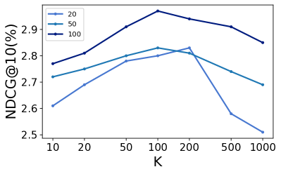
(a) Amazon-RankFlow

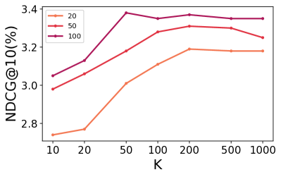
(b) Amazon-CoRR

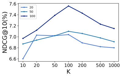
(c) Gowalla-RankFlow

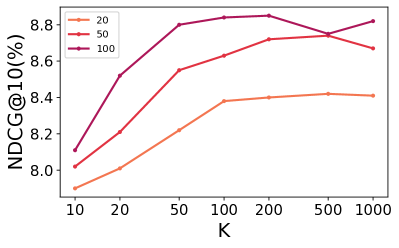
(d) Gowalla-CoRR

Figure 3. Sensitivity w.r.t. Retrieved Items Number

[Sensitivity w.r.t. Retrieved Items Number]Fully described in the Appendix B.4.

B.3. Comparison of Different Distillation Loss

According to results in Section 4.5, knowledge distillation indeed plays an important role in improving the retriever and the whole framework. Ranking-based distillation loss is popular in knowledge distillation in recommendation, which usually attaches larger weights to the items with higher rank. To further study the effectiveness of our distillation loss, we compare several ranking-based distillation strategies with ours. They include:

• RankDistill (Tang and Wang, 2018b): ranks of topk items are used as the weights for negative log likelihood loss.

• CoDistill (Lee et al., 2019): items are sampled by a ranking-based sampling strategy and then a cross entropy loss is used for closing the scores of two models.

The results shown in Table 5 demonstrate that: First, the addition of any one of the three distillation losses is able to enhance the performance of the whole framework. CoDistill loss, whose improvement is smaller, even outperforms w/o Distill with a relative 12.34% improvement on NDCG@10. Besides, our sampled KL loss obviously outperforms the other two losses. Our KL loss achieves 5.86% and 7.19% improvements on Recall@10 compared with RankDistill and CoDistill respectively, indicating the superiority of the asymptotic sampled kl-divergence.

B.4. Sensitivity of the Retrieval Cutoff

As mentioned in Section 4.1.3, a two-stage strategy is applied in prediction: K candidates are retrieved by retriever firstly and then refined by the ranker to get the final recommendation results. The performance may be affected by the retrieval cutoff due to item distribution shift between training and inference of the ranker. To further verify the sensitivity to the retrieval cutoff, we conduct experiments on RankFlow and CoRR by varying the cutoff K in the inference stage within {10, 20, 50, 100, 200, 500, 1000} and varying the number of negatives in {20, 50, 100}. The results are reported in Figure 3(d).

These figures illustrate that the performance gets better as K increases from 10 to 100 for CoRR and RankFlow, which is explained by the limited expressiveness of the retriever. However, the tendencies vary between RankFlow and CoRR when K becomes larger (from 100 to 1000). The performance of CoRR almost holds steady as K increases while RankFlow suffers a severe drop since the rankers face highly shifted item distributions from the training stage. This indicates that CoRR is capable of addressing item distribution shift.

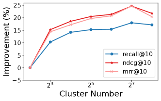
(a) Cluster Number

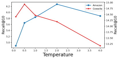
(b) Temperature

Figure 4. Sensitivity w.r.t. Cluster Number and Temperature

[Sensitivity w.r.t. Cluster Number and Temperature]Fully described in the Appendix B.5B.6.

B.5. Sensitivity of the Cluster Number

As mentioned in Section 3.2.2, our scalable and adaptive sampling strategy adopts clustering technique to build index. As the key parameter of clustering, the cluster number (K) would be related to the effectiveness of the sampling. Therefore, we conduct experiments by varing cluster number within {4,8,16,32,64,128,256} on Gowalla. The results are shown in Figure 4(a).

The figure illustrates that as the number of clusters increases, the ranking performance first improves and then saturates. When the cluster number is too small(K=4), there would be amounts of items in the same cluster, which would result in more information loss. When the cluster number is large enough, the performance is relatively insensitive to K.

B.6. Sensitivity of the Temperature

As discussed in Section 3.2.2, temperature T controls the balance between hardness and randomness of negative samples. We conduct experiments on CoRR by varying the temperature T within {0.1,0.5,1,2,4}. The results are reported in Figure 4(b).

When T increases, the sampling distribution is more closed to uniform distribution and the sampler concerns more about randomness. On the contrary, the sampler concerns more about hardness. The results on Amazon and Gowalla dataset show that T=1 is a good option for the final performance.