Meta-Wrapper: Differentiable Wrapping Operator for User Interest Selection in CTR Prediction

Abstract

Click-through rate (CTR) prediction, whose goal is to predict the probability of the user to click on an item, has become increasingly significant in the recommender systems. Recently, some deep learning models with the ability to automatically extract the user interest from his/her behaviors have achieved great success. In these work, the attention mechanism is used to select the user interested items in historical behaviors, improving the performance of the CTR predictor. Normally, these attentive modules can be jointly trained with the base predictor by using gradient descents. In this paper, we regard user interest modeling as a feature selection problem, which we call user interest selection. For such a problem, we propose a novel approach under the framework of the wrapper method, which is named Meta-Wrapper. More specifically, we use a differentiable module as our wrapping operator and then recast its learning problem as a continuous bilevel optimization. Moreover, we use a meta-learning algorithm to solve the optimization and theoretically prove its convergence. Meanwhile, we also provide theoretical analysis to show that our proposed method 1) efficiencies the wrapper-based feature selection, and 2) achieves better resistance to overfitting. Finally, extensive experiments on three public datasets manifest the superiority of our method in boosting the performance of CTR prediction.

1 Introduction

Click-through rate (CTR) prediction plays a centric role in recommender systems, where the goal is to predict the probability that a given user clicks on an item. In these systems, each recommendation returns a list of items that a user might prefer in terms of the prediction. In this way, the performance of the CTR prediction model is directly related to the user experience and thus has a critical influence on the final revenue of an online platform. Therefore, this task has attracted a large number of researchers from the machine learning and data mining community.

Currently, there are many CTR prediction methods [1, 2, 3] that focus on automatic feature engineering. The main idea behind these approaches is learning to combine the features automatically for better representation of instances. Following this trend, recent researches pay particular attention to the interplay of the target item and user behavioral features. Deep Interest Network (DIN) [4] is one of the typical examples. Given a specific user, DIN simply uses an attention layer to locally activate the historically clicked items that are most relevant to the target item. Here the outputs of the attention layer come from the interaction between the given target and each clicked item, characterizing the interests of the user. Similar attentive modules are also used in [5, 6, 7, 8] ,etc. All of these methods capture user interests by means of historically clicked items, under the assumption that user’s preference is covered by one’s behaviors.

Actually, such an attention mechanism can be regarded as a special case of feature selection methods. More specifically, it aims to find the most relevant features (clicked items) according to a given target. Its main difference with traditional feature selection is the membership of features in the subset is not necessarily assessed in binary terms. Here the feature subset could be a fuzzy set and the attention unit can be regarded as the membership function.

However, there exists a fact that is not paid enough attention, namely, feature selection based on attention mechanisms also increase overfitting risks. More specifically, when we regard the attentive module as a feature selector, the other parts of the model are naturally viewed as a base CTR predictor, where the two components are jointly learned from the same training set. Based on this, we can expect that the model with a feature selector is more capable of fitting the training data than using the base predictor only. However, such an approach also introduces additional complexity to the architecture of the predictive model, which implies a higher risk of overfitting. In other words, there is still an improvement space in the generalization performance of those feature selection methods based on attention mechanisms.

Motivated by this fact, we argue that the feature selector should be learned not only from the same data with base predictor, but also from out-of-bag data. In this way, the knowledge learned in feature selector would come from different sources, thus alleviating the possibility of overfitting on a single dataset. Such an idea is exactly inspired by wrapper method [9, 10], which is a classical approach to feature selection. This kind of methods regard feature selection as a non-continuous bilevel optimization (BLO) [11] problem which is shown in Fig.(1a). Instead of solely relying on the training set, the wrapper method takes the performance on the out-of-bag data as the metric of the feature selection. In this way, two datasets with different empirical distribution are utilized during the learning process, thereby mitigating the risk of overfitting.

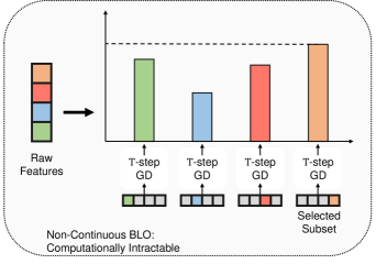
(a) Traditional Wrapper Method

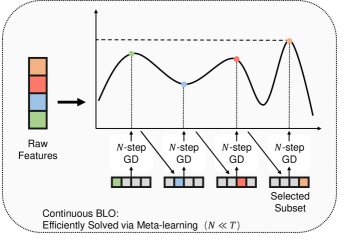
(b) Our Proposed Meta-Wrapper

Figure 1: Comparison between Traditional Wrapper Method and Meta-Wrapper.

However, there are two significant problems left to be solved in traditional wrapper methods:

• Intractable computational complexity: The number of possible feature combinations increases exponentially with feature dimensions. Therefore, it is actually an NP-hard problem to find the best feature subset. To get an acceptable selection result, the model must be trained again and again on different feature subsets, which leads to a great computing cost.

• Insufficient flexibility: In CTR prediction, the selection of the features (clicked items) should rely on the target item, which cannot be directly implemented via traditional wrapper methods. Meanwhile, wrapper methods search the best feature combination in discrete space instead of continuous space. Thus it cannot be used as a differentiable sub-module, like attention mechanisms, of an end-to-end deep learning model.

In order to solve these problems, we propose a novel feature selection approach under the framework of the wrapper methods, which is called Meta-Wrapper. Our main idea is to encapsulate the inner-level learning process by means of a differentiable wrapping operator. By applying this operator, the wrapper-based feature selection is recast to a continuous BLO problem that can be efficiently solved through meta-learning [12]. To this end, we, following the similar spirit of attention methods, regard the feature selection problem as learning a scoring function. This function takes behavioral features and the target item as inputs, then outputs the relevant scores used for properly selecting features. More specifically, the novelty of our proposed method can be viewed from two perspectives:

• As is shown in Fig.(1), our feature selector could be meta-learned in a more efficient manner compared with the traditional wrapper method. We will elaborate on this meta-learning algorithm and its convergence result in the following sections.

• Compared with attention mechanisms, our feature selector is learned from two different sources. This actually leads to an implicit regularization term to prevent overfitting. In later sections, we also provide theoretical analysis on this point.

In other words, our work bridges the gap between deep-learning-based feature selector and classical wrapper method, in the sense that the generalization ability of the feature selector can be improved through an efficiently meta-learned wrapping operator.

To summarize, the main contributions of this paper are three-fold:

• We propose a novel approach to user interest selection, which encapsulates the optimizing iterations by means of a differentiable wrapping operator. Such an approach unifies feature selection and CTR prediction into a continuous BLO objective.

• From theoretical analysis, we show that there exists an implicit regularization term in such a BLO objective, which explains how this objective alleviates overfitting.

• We develop a meta-learning algorithm for solving this BLO problem in an efficient way. Taking a step further, we theoretically prove the convergence of this algorithm under a set of broad assumptions.

2 Related Work

2.1 CTR prediction

As an early trial, researchers solve the CTR prediction problem mainly through simple models with expert feature engineering. [13] integrates multiple discrete features and trains a linear predictor through an online sparse learning algorithm. [14] introduces a machine learning framework based on Logistic Regression, aiming to predict CTR for online ads. [15] ensembles collaborative filters, probability models and feature-engineered models to estimate CTR. [16] uses ensembled decision trees to capture the features of social ads, thereby improving the model performance. In spite of the remarkable success of these models, they heavily rely on manual feature engineering, which results in significant labor costs for developers.

To address this problem, Factorization Machines (FM) [17] are proposed to automatically perform the second-order feature-crossing by inner production of feature embeddings. More recently, [18, 19, 20, 21, 22, 23, 24, 25] improve the FM model from different perspectives, for the sake of better predictive performance. Notably, such embedding mechanisms have better resistance to the sparsity of crossed features since the embedding for each individual feature is trained independently. To capture more sophisticated feature interactions, there is a line of works using the universal approximation ability of Deep Neural Networks (DNN) to improve the feature embedding. Deep crossing model [26] feeds the feature embeddings into a cascade of residual units [27]. Moreover, Factorization-machine supported Neural Network (FNN) [28] stacks multiple dense layers on top of an embedding layer transferred from a pre-trained FM. Based on a similar architecture, Product-based Neural Network (PNN) [1] adds a product layer between the embedding layer and the dense layers. Following a similar spirit, Neural Factorization Machine (NFM) [29] adds a bi-interaction layer before the dense layers to enhance the embeddings, thereby achieving state-of-the-art performance via fewer layers. It is equivalent to stack dense layers on a second-order FM. More recently, [30] automatically learns the high-order feature interactions by multi-head self-attention [31], which is called Automatic Feature Interaction Learning (AutoInt). By leveraging the ability of representation learning, these models implement automatic feature-crossing in CTR prediction. There is also another line of works that consider low- and high-order feature-crossing simultaneously. The well-known Wide&Deep model [32] captures low- and high-order feature-crossing in terms of wide and deep components, respectively. After this work, there emerge some related researches that improve the wide or deep component. DeepFM [2] uses second-order FM as the wide component to automatically capture low-order feature-crossing. [33] proposes a model named Field-aware Probabilistic Embedding Neural Network (FPENN). It uses field-aware probabilistic embedding (FPE) strategy to enhance the wide and deep components simultaneously. Moreover, Deep & Cross Network (DCN) [34] utilizes a cross network as the wide component, for modeling the N-order feature-crossing in a more efficient way. [3] proposes eXtreme Deep Factorization Machine (xDeepFM). It uses a Compressed Interaction Network (CIN) as the wide component, thereby improving the representative ability compared with DCN. Taking a step further, [35] uses graph neural networks (GNN) with adversarial training strategy to capture more complex feature relations. This method successfully achieves robustness towards the perturbations. Additionally, [36] proposes a novel method to capture interest features for cold-start users, which achieves state-of-the-art performance in this setting. All of these methods clearly show the effectiveness of automatic feature engineering in this area.

Different from the previous research, recent methods pay more attention to model users’ interest by using behavioral features. Notably, feature interaction and user interest modeling are not contradictory to each other. The latter is mainly an approach to deal with behavior feature sequences. Deep Interest Network (DIN) [4] uses attention mechanisms to adaptively activate user interests for a given item, where the user interests are modeled as his/her clicked items. This method adaptively produces the user interest representation by selecting the most relevant behaviors to the target item. In other words, the user representation varies over different targets, thus improving the expressive ability. Deep Interest Evolution Network (DIEN) [5] designs an RNN-based module as an interest extractor to model the user interest evolution. Deep Session Interest Network (DSIN) [6] splits the users’ behavioral sequences as multiple sessions, for modeling their interest evolution at session-wise level. [7] proposes a model named Hierarchical Periodic Memory Network (HPMN). This model uses memory networks to incrementally capture dynamic user interests. Similarly, Multi-channel user Interest Memory Network (MIMN) [8] also takes the memory network to capture the long-term user interests and designs a separate module named User Interest Center (UIC) to reduce the latency of online serving. All these models are developed from the basis of DIN, improving the user interest modeling from the time series perspective.

Following these works, we also focus on capturing the interests in the user behavioral features. However, we recast the user modeling as a feature selection problem rather than capturing the user interest evolution, which provides a novel perspective for the CTR prediction task.

2.2 Feature Selection

Feature selection methods can be normally divided into three categories: filter, wrapper, and embedded methods [37, 38]. In this section, we will discuss the three kinds of methods respectively. Filter methods rank the features by their related scores to the target. Different filter approaches adopt various kinds of metrics to score the relevance, such as T-score [39], information-theory based criteria [40], similarity metrics [41], and fisher-score [42] .etc. These methods can only select the relevant features by some pre-defined rules, leading to the inability to adaptively modulate selected results. Wrapper methods [10] compare validating performances of the models with different feature subsets. To this end, the model must be repeatedly trained for every possible subset, resulting in intractable computational complexity [9]. In this way, wrapper methods are not desirable for the tasks with large-scale datasets, such as recommender systems. In the embedded methods, a feature selector is jointly learned with the predictive model, which has more efficiency than the wrapper methods. In an early trial, there exist many approaches that penalize weights of irrelevant features via specific regularization terms. [43] uses $L_{2,1}$-norm to learn sparse feature weights, where the weights of irrelevant features are reduced to zero. for the sake of better flexibility, [44] uses the probabilistic $L_{2,1}$-norm to select features, where feature subset can be different for various targets. With the popularity of deep learning, there emerge another kind of embedded methods based on neural networks, which are called attention mechanisms [45]. This strategy is widely applied in many areas, such as object detection [46, 47, 48, 49], machine translation [45, 31], video description [50] and diagnosis prediction [51]. All of these methods use attentive modules to produce real-valued weights to capture feature importance. To obtain discrete feature subsets, [52] and [53] design special attentive modules which provide sparse weights. However, the sparsity of the selected subset, for recommender systems, is actually less important than its representative ability.

In this paper, we follow the spirit of the wrapper and embedded method simultaneously. We model the feature selector as a neural network meta-learned jointly with base predictor, thereby avoiding excessive computing costs. Meanwhile, flexibility can also be taken into account to handle the diversity of user interests.

3 Problem Statement

We commence by introducing deep-learning based CTR prediction. Then we formulate the user interest selection problem in this field. Notations defined in this section will be adopted in the entire paper. More notations and their descriptions are listed in Appendix.

3.1 Deep-Learning Based CTR Prediction

To define the user interest selection, we first need to formulate the CTR prediction task. Given a set of triples $\{({u},{v},{y})\}$ each of which includes the user $u\in\mathcal{U}$, item $v\in\mathcal{V}$ and the corresponding label of user click indicator

$${y}=\left\{\begin{array}[]{lr}1,\ \ {u}\ has\ clicked\ {v};\\ 0,\ \ otherwise,\\ \end{array}\right.$$

our goal is to predict click-through rate $\hat{{p}}({y}=1|{u},{v})$. Here the $({u},{v})$ are indices of the user and target item, while other inputs are omitted for their non-directly relevance to our problem. We implement CTR prediction through a learned function $f_{\bm{\theta}}(\cdot)$ with parameters $\bm{\theta}$, which can be simply formulated as

$$\hat{{p}}({y}=1|{u},{v})=f_{\bm{\theta}}({u},{v}).$$

To learn $f_{\bm{\theta}}(\cdot)$, the cross-entropy loss $L({y},\hat{{p}})$ is used as the optimization target

$$L({y},\hat{{p}})=-{y}\log(\hat{{p}})-(1-{y})\log(1-\hat{{p}}).$$ (1)

Consider that $f_{\bm{\theta}}(\cdot)$ is usually modeled as a deep neural network and $L({y},\hat{{p}})$ would be optimized by the algorithms with gradient operations. The categorical inputs of $f_{\bm{\theta}}(\cdot)$ have to be transformed into real-value vectors through an embedding layer. More formally, the predictive model can be further represented as

$$\hat{{p}}({y}=1|{u},{v})=f_{\bm{\theta}}(\bm{\theta}^{E}_{u},\bm{\theta}^{E}_{v}),$$ (2)

where $\bm{\theta}^{E}\in\mathbb{R}^{{K}\times{M}}$ is the embedding matrix; ${M}$ is the number of categorical features in all; ${K}$ is the dimension of each embedding vector; $(\bm{\theta}^{E}_{u},\bm{\theta}^{E}_{v})$ are embeddings of the user ${u}$ and target item ${v}$, respectively.

3.2 Exploiting User Behavioral Features

From Eq.(2), we observe that traditional CTR prediction methods simply represent each user as a ${K}$-dimensional embedding vector. However, recent works [54] find such a method seems insufficient for learning user preference in real-world recommender systems.

for the sake of better representation, augmenting the user with his/her historical features [4, 55, 56] has become a widely adopted paradigm. More Specifically, historical features of a user naturally refer to the sequence of his/her clicked items. Based on this, we can represent each user ${u}$ as

$$\bm{r_{{u}}}=[\bm{\theta}^{E}_{v_{1}};\bm{\theta}^{E}_{v_{2}};\cdots\bm{\theta}^{E}_{v_{T_{u}}}],$$ (3)

where $\bm{r_{{u}}}\in\mathbb{R}^{{K}\times{T_{u}}}$ represents the user’s behavioral sequence; ${T_{u}}\in\mathbb{N}^{+}$ is the number of clicked items; ${v_{1}}\dots v_{T_{u}}$ are clicked items; each $\bm{\theta}^{E}_{v_{.}}\in\mathbb{R}^{{K}}$ is the embedding of a clicked item.

In this way, a CTR prediction model with user behavioral features can be formulated as

$$\hat{{p}}({y}=1|{u},{v})=f_{\bm{\theta}}(\texttt{Pooling}(\bm{r_{{u}}}),\bm{\theta}^{E}_{v}),$$ (4)

where $\texttt{Pooling}(\bm{r_{{u}}})\in\mathbb{R}^{{K}}$ is the result of applying a pooling function to user representation. By taking the behavioral features into account, we replace $\bm{\theta}^{E}_{u}$ in Eq.(2) with a more comprehensive user representation $\bm{r_{{u}}}$.

3.3 Modeling User Interest by Feature Selection

Despite that introducing behavioral features could enhance user representation, there is a fact that the number of clicked items is continually growing over time. With this trend, some user’s behavioral sequence would become extremely long. In this scene, not all historical behaviors can play a positive role in every specific prediction. For example, when a user shopping for clothes on the e-commerce platform, it is totally irrelevant to which books he/she bought in the past.

Therefore, we need to filter out the non-trivial items from each user’s behavioral sequence, keeping the items that are beneficial to downstream prediction. Since the remaining items are considered more representative for user interest, we name such a process as user interest selection. Essentially, it can be regarded as a special case of feature selection problems.

More formally, our goal is to learn a function $g_{\bm{\phi}}(\cdot)$ with parameter $\bm{\phi}$ for selecting user interests:

$$\bm{s_{{u}}}=g_{\bm{\phi}}(\{\bm{\theta}^{E}_{v_{i}}\}_{{i}=1}^{T_{u}},\bm{\theta}^{E}_{v}),$$ (5)

where $\bm{\theta}^{E}_{v}$ is the embedding of the target item; $\bm{s_{{u}}}\in\mathbb{R}^{{T_{u}}}$ represents the relevant scores between each behavioral feature and the target ${v}$:

$$\left\{\begin{array}[]{lr}\bm{s_{{u}}}[i]>\bm{s_{{u}}}[j],\ \ {v_{i}}\ is\ more\ relevent\ to\ {v};\\ \bm{s_{{u}}}[i]<\bm{s_{{u}}}[j],\ \ {v_{j}}\ is\ more\ relevent\ to\ {v};\\ \bm{s_{{u}}}[i]=\bm{s_{{u}}}[j],\ \ otherwise.\\ \end{array}\right.$$

Similar to [57] and [4], we take the inner product

$$\bm{\hat{r}_{{u}}}=(\bm{r_{{u}}}\bm{s_{{u}}})\in\mathbb{R^{{K}}}$$

as the aforementioned pooling function. In other words, it is a weighted sum of all feature embeddings $\bm{r_{{u}}}$, where the weights $\bm{s_{{u}}}$ is the relevance between the features and the target. Moreover, if we would like to highlight the most related behavioral feature, $\bm{\hat{r}_{{u}}}$ can also be represented as

$$\bm{\hat{r}_{{u}}}=\texttt{softmax}(\bm{r_{{u}}}\bm{s_{{u}}})\in\mathbb{R^{{K}}}.$$

Based on this, a CTR prediction model with user interest selection can be formulated as

$$\hat{{p}}({y}=1|{u},{v})=f_{\bm{\theta}}(\bm{\hat{r}_{{u}}},\bm{\theta}^{E}_{v}),$$ (6)

where $\bm{s_{{u}}}$ is produced by $g_{\bm{\phi}}(\cdot)$ as Eq.(5).

Notably, the relationship between $g_{\bm{\phi}}(\cdot)$ and $f_{\bm{\theta}}(\cdot)$ in this paper is a little different from other works. In most other work, $f_{\bm{\theta}}(\cdot)$ represents the whole model and $g_{\bm{\phi}}(\cdot)$ is merely its component. On the contrary, we regard $f_{\bm{\theta}}(\cdot)$ as a base predictor that can be applied with arbitrary feature selector $g_{\bm{\phi}}(\cdot)$. They are viewed as two independent modules that can be trained jointly or separately.

4 Motivation

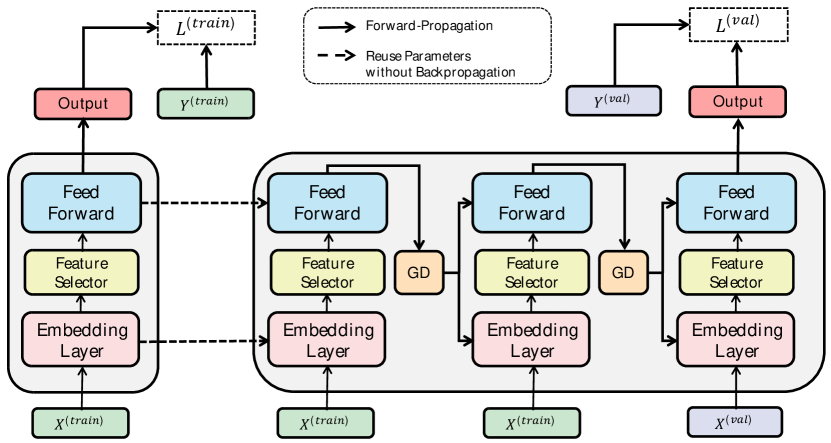
Figure 2: Overview of Meta-Wrapper Method (${N}=2$ for Example).

Normally, the feature selector $g_{\bm{\phi}}(\cdot)$ is modeled as an attention network that locally activates some behavioral features according to the target item [4]. Such an attention mechanism actually enhances the ability to fit the training data. Unfortunately, it also increases the overfitting risk, due to the over-parameterization. Motivated by this fact, we first go back to a classical feature selection approach, i.e., wrapper method [9]. In this method, the feature selector is not learned from the training set, but from out-of-bag data. By incorporating the knowledge from different sources, it leads to a better generalization performance.

Corresponding to user interest selection, the goal of the wrapper method can be formally represented as the following bilevel optimization [11]:

$$\mathop{\arg\min}_{\bm{\phi}}\ L^{(out)}(\bar{\bm{\theta}},\bm{\phi}),$$ (7)

$$\ \ s.t.\ \bar{\bm{\theta}}=\mathop{\arg\min}_{\bm{\theta}}\ L^{(in)}(\bm{\theta},\bm{\phi}),$$

where $L^{(\cdot)}(\cdot,\cdot)$ is the cross-entropy loss Eq.(1) with label ${y}$ and prediction $\hat{{p}}$ yield by Eq.(6); superscripts $(in)$ and $(out)$ indicate the training (in-the-bag) and out-of-bag data $\mathcal{D}^{(in)}$ and $\mathcal{D}^{(out)}$ that are also called inner- and outer-level dataset in this paper; $\bar{\bm{\theta}}$ represents the parameters of an optimal $f_{\bm{\theta}}(\cdot)$ w.r.t a predefined $g_{\bm{\phi}}(\cdot)$. For such a method, the feature selection is motivated by the need for generalization well to out-of-bag data $\mathcal{D}^{(out)}$.

Remark 1 (Feature Selector in Wrapper Method).

Notably, canonical wrapper methods restrict the feature selector as a learnable indicating vector:

$$g_{\bm{\phi}}(\{\bm{\theta}^{E}_{v_{i}}\}_{{i}=1}^{T_{u}},\bm{\theta}^{E}_{v})=\bm{\phi}_{{u},{v}}\in\{0,1\}^{{T_{u}}}$$

which is defined as

$$\bm{\phi}_{{u},{v}}[{i}]=\left\{\begin{array}[]{lr}1,\ \ {u}\ has\ clicked\ {v_{i}};\\ 0,\ \ otherwise.\\ \end{array}\right.$$

Obviously, such a simple model is incapable of producing different relevant scores depending on different target items. Thus it is not suitable for user interest selection tasks. For a fair comparison with other methods, we will relax this restriction in this paper, allowing the use of neural networks as feature selectors.

Unfortunately, the wrapper method actually cannot be directly applied to our problem, since its computational complexity is unacceptable. To explain, we provide the following example.

Example 1 (GDmax-Wrapper).

Given a user ${u}$ and target item ${v}$, we are required to find an optimal feature selector $g_{\bm{\phi}}(\cdot)$ by solving the problem Eq.(7). for the sake of sufficient flexibility, $g_{\bm{\phi}}(\cdot)$ is modeled as a neural network. Now we reverse the inner minimization as its equivalent maximization. Thus Eq.(7) is reformulated as the following:

$$\mathop{\arg\min}_{\bm{\phi}}\ L^{(out)}(\bar{\bm{\theta}},\bm{\phi}),$$

$$\ \ s.t.\ \bar{\bm{\theta}}=\mathop{\arg\max}_{\bm{\theta}}\ \left(-L^{(in)}(\bm{\theta},\bm{\phi})\right).$$

Following the paradigm of traditional wrapper method, we first get a sufficiently precise inner solution $\bar{\bm{\theta}}$ by performing gradient descent on $\bm{\theta}$ until $L^{(in)}$ converges. Based on the inner solution, we solve the outer problem by optimizing $\bm{\phi}$. We find this process is quite similar to GDmax algorithm [58]. Borrowing this concept, we call such a wrapper method as GDmax-Wrapper.

In this case, whenever we calculate $\bar{\bm{\theta}}$, we must scan the entire training set to solve the inner maximization. Assume that we need to perform $T^{(in)}$ loops of gradient ascent (GA) for inner maximization and $T^{(out)}$ loops of gradient descent (GD) for outer minimization. Let $T^{(all)}$ notate the total number of gradient descent/ascent loops. To find the optimal feature selector in Example.(1), we have $\mathbb{E}(T^{(all)})=\mathcal{O}(T^{(in)}\times T^{(out)})$, where the computational complexity is unbearable.

5 Methodology

In this section, we propose a differentiable wrapper method, i.e., Meta-Wrapper, for user interest selection in CTR prediction. Specifically, we first illustrate two points about the Meta-Wrapper:

• How to recast traditional wrapper method Eq.(7) to a continuous bilevel optimization problem;

• How our $g_{\bm{\phi}}(\cdot)$ and $f_{\bm{\theta}}(\cdot)$ are jointly trained by using our proposed method.

After that, we theoretically analyse how our proposed method prevents overfitting. Finally, we detail our network architecture.

5.1 Differentiable Wrapping Operator

Under the framework of the wrapper method, we model the user interest selection as a bilevel optimization Eq.(7). Unfortunately, such a problem is hardly solved in an efficient way since its objective function is non-differentiable. Recalling the analysis about our Example.(1), we know the reason lies in the inner-level argmin function. With this obstacle, whenever we compute the outer-level loss, $\bm{\theta}$ must be trained from scratch, leading to great computational costs.

However, if we approximate the inner-level argmin as a differentiable function, then the losses in both levels could be jointly optimized. This will bring a great improvement in efficiency. To this end, we regard the learning process of the inner-level problem in Eq.(7) as a learnable function from the meta-learning [59] perspective. By expanding its optimizing rollouts, we can recast Eq.(7) as a continuous bilevel optimization.

More specifically, we first define a function ${U}_{\bm{\phi}}(\cdot)$ so that ${U}_{\bm{\phi}}(\bm{\theta},\mathcal{D}^{(in)})$ is a result of ${N}$-step gradient descent (GD) on dataset $\mathcal{D}^{(in)}$ for minimizing the inner loss:

$${U}_{\bm{\phi}}(\bm{\theta},\mathcal{D}^{(in)})=\bm{\theta}^{({N})},$$ (8)

where $\bm{\theta}^{({N})}$ is the optimal parameters at inner level. To calculate $\bm{\theta}^{({N})}$, each GD step is performed as

$$\bm{\theta}^{(j)}=\bm{\theta}^{(j-1)}-\beta\nabla_{\bm{\theta}^{(j-1)}}L^{(in)}(\bm{\theta}^{(j-1)},\bm{\phi}),$$ (9)

where each $j\in\{1,\dots,{N}\}$ denotes the step number, thus $\bm{\theta}^{(0)}$ represents the initial value of $\bm{\theta}$; $\beta>0$ is the inner-level learning rate.

Based on this, the objective function of the wrapper method Eq.(7) can be recast to the following continuous optimization:

$$\mathop{\arg\min}_{\bm{\phi}}\ L^{(out)}(\bar{\bm{\theta}}(\bm{\phi}),\bm{\phi}),$$ (10)

$$\ \ s.t.\ \bar{\bm{\theta}}(\bm{\phi})={U}_{\bm{\phi}}(\bm{\theta},\mathcal{D}^{(in)}),$$

where the inner-level argmin has been approximated as

$$\mathop{\arg\min}_{\bm{\theta}}\ L^{(in)}(\bm{\theta},\bm{\phi})\approx{U}_{\bm{\phi}}(\bm{\theta},\mathcal{D}^{(in)}).$$ (11)

Based on Eq.(8) and Eq.(9), the computing process of $\bar{\bm{\theta}}(\bm{\phi})={U}_{\bm{\phi}}(\bm{\theta},\mathcal{D}^{(in)})$ can be formulated as Alg.1.

Algorithm 1 Inner-level Optimization as ${U}_{\bm{\phi}}(\cdot)$

Input: initial value $\bm{\theta}^{(0)}$
    Input: Training data $\mathcal{D}^{(in)}$
    Output: ${N}$-step GD result $\bm{\theta}^{({N})}$ depending on $\bm{\phi}$

1:  Detach Operation: $\bm{\theta}^{\prime}:=\bm{\theta}^{(0)}$;

2:  for $j\leftarrow 1$ to ${N}$ do

3:     $\texttt{Grad}(\bm{\theta}^{\prime}):=\nabla_{\bm{\theta}^{\prime}}L^{(in)}(\bm{\theta}^{\prime},\bm{\phi})$;

4:     $\bm{\theta}^{(j)}:=\bm{\theta}^{\prime}-\beta\cdot\texttt{Grad}(\bm{\theta}^{\prime})$;

5:     $\bm{\theta}^{\prime}:=\bm{\theta}^{(j)}$;

6:  end for

7:  return  $\bm{\theta}^{({N})}$;

Notably, Alg.1 is a functional process where the value of $\bm{\theta}$ would not be changed. Each GD-step is actually performed on a newly created node in the computational graph. Hence we can apply the chain rule over its nested GD-loops to calculate $\nabla_{\bm{\phi}}{U}_{\bm{\phi}}(\bm{\theta},\mathcal{D}^{(in)})$, which is shown in Alg.2.

Algorithm 2 backpropagation of ${U}_{\bm{\phi}}(\cdot)$

Input: $\{\bm{\theta}^{({1})},\dots,\bm{\theta}^{({N})}\}$
    Output: $\nabla_{\bm{\phi}}\left({U}_{\bm{\phi}}(\bm{\theta},\mathcal{D}^{(in)})\right)$

1:  Set $b:=\nabla_{\bm{\phi}}{U}_{\bm{\phi}}(\bm{\theta}^{({N})},\bm{\phi})$

2:  for $j\leftarrow{N}$ to $1$ do

3:     Set $a:=\bm{\theta}^{({j})}$;

4:     Set $b:=b-\beta(\nabla^{2}_{a,\bm{\phi}}{U}_{\bm{\phi}}(a,\bm{\phi}))^{\top}b$;

5:  end for

6:  return  $b$;

In this way, we can regard ${U}_{\bm{\phi}}(\cdot)$ as a learnable meta-model [60] with parameters $\bm{\phi}$. The meta-model takes a base predictor as input then generates another one that has been sufficiently trained. Under the framework of the wrapper method, we call this meta-model as our differentiable wrapping operator. More intuitively, It is demonstrated as the biggest gray box in Fig.(2). Without using additional parameters other than $\bm{\phi}$, learning ${U}_{\bm{\phi}}(\cdot)$ by minimizing Eq.(10) is equivalent to learning feature selector $g_{\bm{\phi}}(\cdot)$. Therefore, we call such a feature selection strategy as Meta-Wrapper method and Eq.(10) as Meta-Wrapper loss.

5.2 Jointly Learning With Base Predictor

Recall that our predictive model consists of two components, i.e., the base predictor $f_{\bm{\theta}}(\cdot)$ and user interest selector $g_{\bm{\phi}}(\cdot)$. To obtain the completed model, we still have to learn parameters $\bm{\theta}$ in addition to $\bm{\phi}$.

To this end, we unify the original cross-entropy loss and Eq.(10) as the final loss function:

$$\mathop{\arg\min}_{(\bm{\theta},\bm{\phi})}\ \mathcal{L}(\bm{\theta},\bm{\phi})=L^{(in)}(\bm{\theta},\bm{\phi})+\mu L^{(out)}(\bar{\bm{\theta}}(\bm{\phi}),\bm{\phi}),$$ (12)

$$\ \ s.t.\ \bar{\bm{\theta}}(\bm{\phi})={U}_{\bm{\phi}}(\bm{\theta},\mathcal{D}^{(in)}),$$

where $\mu\in[0,1]$ is a coefficient to balance the CTR prediction and user interest selection. If we set $\mu=0$, the Meta-Wrapper loss then disappears and it degrades into an ordinary CTR prediction method with an attentive feature selector.

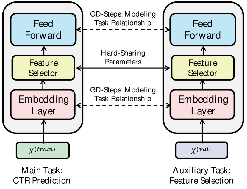
Figure 3: Multi-Task Learning Perspective.

From the multi-task learning perspective, we can regard CTR prediction as our main task and user interest selection as a corresponding auxiliary task. Each task could transfer its learned knowledge to the other, thus all tasks can be improved simultaneously. This is shown in Fig.(3). Compared with the traditional wrapper, our proposed method explicitly models the task relationship by inner GD-loops, which is a more fine-grained manner than hard sharing the parameters.

For optimizing Eq.(12), the first step is to calculate $\bar{\bm{\theta}}(\bm{\phi})$ at inner level. After that, we plug the result into the outer-level loss and then perform minimization. Thanks to the differentiability of ${U}_{\bm{\phi}}(\cdot)$, this problem can be efficiently solved by adopting mini-batch gradient descent [61] as our optimizer. Specifically, we can perform inner-level optimization as Alg.1. By virtue of this, the optimal $\bm{\theta}$ and $\bm{\phi}$ can be obtained by minimizing the outer-level loss as Alg.3, where the $\bm{\gamma}_{i}$ is the outer-level learning rate such that $\lim_{i\rightarrow\infty}\gamma_{i}=0$ and $\sum_{i=1}^{\infty}\gamma_{i}=\infty$. Meanwhile, Alg.2 performs as an intermediate node in the computing graph when calculating the gradient $\nabla_{(\bm{\theta},\bm{\phi})}{\mathcal{L}(\bm{\theta},\bm{\phi})}$ in Alg.3. Here the combination of $\{\mathcal{D}^{(in)},\mathcal{D}^{(out)}\}$ can be viewed as a meta-learning task $\mathcal{T}$. We represent the distribution of $\mathcal{T}$ as $\mathcal{P}(\mathcal{T})$ for the convenience of further analysis.

Algorithm 3 Solving Eq.(12) by Mini-batch GD

Input: Entire Inner-level Dataset $\bm{\Omega}^{(in)}$
    Input: Entire Outer-level Dataset $\bm{\Omega}^{(out)}$
    Input: Initial parameters $\bm{\phi}_{(0)},\bm{\theta}_{(0)}$
    Input: Number of epochs ${T}\in\mathbbm{N}$
    Output: Learned parameters $\bm{\phi}_{({T})},\bm{\theta}_{({T})}$

1:  Set $\bm{\phi}:=\bm{\phi}_{(0)}$;

2:  Set $\bm{\theta}:=\bm{\theta}_{(0)}$;

3:  for $i\leftarrow 1,2,\ldots,{T}$ do

4:     $\mathcal{D}^{(in)}\leftarrow$ Draw a batch from $\bm{\Omega}^{(in)}$;

5:     $\mathcal{D}^{(out)}\leftarrow$ Draw a batch from $\bm{\Omega}^{(out)}$;

6:     $\mathcal{L}(\bm{\theta},\bm{\phi}):=L^{(in)}(\bm{\theta},\bm{\phi})+\mu L^{(out)}(\bar{\bm{\theta}}(\bm{\phi}),\bm{\phi})$;

7:     $(\bm{\theta}_{(i)},\bm{\phi}_{(i)}):=(\bm{\theta},\bm{\phi})-\gamma_{i}\nabla_{(\bm{\theta},\bm{\phi})}{\mathcal{L}(\bm{\theta},\bm{\phi})}$;

8:     Set $\bm{\phi}:=\bm{\phi}_{(i)}$;

9:     Set $\bm{\theta}:=\bm{\theta}_{(i)}$;

10:  end for

11:  return  $\bm{\phi}_{({T})},\bm{\theta}_{({T})}$

5.3 Convergence Result

In this section, we provide the convergence result of Alg.3 under a set of broad assumptions. We find this algorithm could reach a stationary point of the objective of our proposed method Eq.(12). More formally, the algorithm would find a solution such that

$$\lim_{i\rightarrow\infty}\|\nabla_{\bm{z}}\mathcal{F}_{i}\|^{2}=0,$$ (13)

where $\|\cdot\|$ represents the $L_{2}$-norm; $\bm{z}=[\bm{\theta}^{\top},\bm{\phi}^{\top}]^{\top}\in\mathbb{R}^{p}$ represents all of the parameters; $\bm{z}_{(i)}$ is the value of the parameters after $i$th-step of outer-level GD, namely, line:$7$ in Alg.3; $\mathcal{F}_{i}$ represents $\mathbb{E}_{p(\mathcal{T})}({\mathcal{L}(\bm{z}_{(i)})})$. This equation means that there exists an iteration of Alg.3, which approaches a stationary point to any level of proximity. More specifically, we first provide the assumption used for our proofs.

Assumption 1.

For any mini-batch data $\mathcal{D}^{(in)}$ or $\mathcal{D}^{(out)}$, $L^{(\cdot)}(\bm{z})$ are second-order differentiable as the function of $\bm{z}$, where $L$ is the cross-entropy loss on top of a neural network. Given arbitrary $\bm{z},\bm{z}_{w},\bm{z}_{u}\in\mathbb{R}^{p}$, there are constants $C_{0},C_{1},C_{2}>0$ such that for any mini-batch data, we have

1. $\|\nabla_{\bm{z}}L^{(\cdot)}(\bm{z})\|\leq C_{0}$;

2. $\|\nabla^{2}_{\bm{z}}L^{(\cdot)}(\bm{z})\|\leq C_{1}$;

3. $\|\nabla^{2}_{\bm{\bm{z}}}L^{(\cdot)}(\bm{z}_{w})-\nabla^{2}_{\bm{\bm{z}}}L^{(\cdot)}(\bm{z}_{u})\|\leq C_{2}\|\bm{z}_{w}-\bm{z}_{u}\|$.

With this assumption, we can provide a convergence analysis in the sense that a stationary point can be achieved within a finite number of iterations via Alg.3. The readers are referred to Appendix for the proof of theorem.

Theorem 1 (Convergence Result of Alg.3).

Let $\mathcal{L}$ be the loss function defined as Eq.(12), $L^{(in)}$ and $L^{(out)}$ be cross-entropy loss satisfying Assumption.(1), $C_{r}>0$ be a positive constant. Denote parameters $\bm{z}\in\mathbb{R}^{p}$ such that $\|\bm{z}\|^{2}<C_{r}$, $C_{3}=N\beta C_{2}(\sqrt{p}+\beta C_{1})^{{N}-1}C_{0}$, $C_{L1}=2C_{1}+\mu C_{3}$, $C_{L2}=C^{2}_{0}+\mu(\sqrt{p}+\beta C_{1})^{{2N}}C_{0}^{2}$, $C_{L3}=\frac{C_{L1}}{2}(C^{2}_{0}+C_{L2})$. Moreover, let $\{\bm{z}_{(i)}\}_{i=1}^{\infty}$ be the parameters sequence generated by applying Alg.3 for optimizing $\mathcal{L}(\bm{z})$, $\mathcal{F}_{i}=\mathbb{E}_{p(\mathcal{T})}({\mathcal{L}(\bm{z}_{(i)})})$, $\{\gamma_{i}>0\}_{i=1}^{\infty}$ be the sequence of outer-level learning rate. Then it holds that

1. If $\forall i\in\mathbb{N}:\gamma_{i}<2\frac{C^{2}_{0}+C_{L2}}{C_{L3}}$ , then $\{\mathcal{F}_{i}\}_{i=1}^{\infty}$ is a non-increasing sequence.

2. If $\sum_{i=1}^{\infty}\gamma_{i}^{2}<\infty$, then $\lim_{i\rightarrow\infty}\|\nabla_{\bm{z}}\mathcal{F}_{i}\|^{2}=0$ and there exists a subsequence of $\{\bm{z}_{s_{i}}\}_{i=1}^{\infty}$ that converges to a stationary point.

3. If $\forall k\in\mathbb{N}:\gamma_{k}=k^{-0.5}$, then for any $\epsilon>0$ we can get that $\min_{0\leq j<k}\|\nabla_{\bm{z}}{\mathcal{F}_{j}}\|^{2}=\bm{\Omega}(k^{-0.5+\epsilon})$.

5.4 Implicit Regularization

In this section, we explore how our proposed Meta-Wrapper loss Eq.(10) alleviates overfitting while learning the user interest selector.

Recall that our model consists of two components 1) base predictor, and 2) user interest selector, i.e., wrapping operator, that is used to select user interested features (items). We use $\bm{\theta}$ and $\bm{\phi}$ to represent vectorized parameters of these two components, respectively. For the convenience of further analysis, we define

$$G_{\bm{\theta}}(\bm{\phi})=\nabla_{\bm{\theta}}{L^{(in)}(\bm{\theta},\bm{\phi}})$$

and

$$G^{\prime}_{\bm{\theta}}(\bm{\phi})=\nabla_{\bm{\theta}}{L^{(out)}(\bm{\theta},\bm{\phi}})$$

in this section.

Now let us analyse the Meta-Wrapper loss. With the inner gradient descent at the $k$-th step

$$\bm{\bm{\theta}}^{(k)}=\bm{\bm{\theta}}^{(k-1)}-\beta G_{\bm{\bm{\theta}}^{(k-1)}}(\bm{\phi}),$$ (14)

the outer loss can be reformulated as

$$L^{(out)}(\bar{\bm{\theta}}^{(N)},\bm{\phi})$$ (15)

$$= L^{(out)}(\bm{\theta}^{{(N-1)}}-\beta G_{\bm{\bm{\theta}}^{{(N-1)}}}(\bm{\phi}),\bm{\phi})$$

where ${N}$ is the total number of inner updating loops.

Then we can consider what Eq.(15) could do for better resistance towards overfitting. We take the first-order Taylor expansion of $L^{(out)}(\bar{\bm{\theta}},\bm{\phi})$ with respect to parameter $\bm{\theta}$ on $\bm{\theta}=\bm{\theta}^{(N)}$, yielding the following equation:

$$L^{(out)}(\bm{\theta}^{{(N-1)}}-\beta G_{\bm{\bm{\theta}}^{{(N-1)}}}(\bm{\phi}),\bm{\phi})$$ (16)

$$\approx L^{(out)}({\bm{\theta}}^{(N-1)},\bm{\phi})-\beta G_{\bm{\theta}^{({N-1})}}^{\top}(\bm{\phi})G^{\prime}_{\bm{\theta}^{({N-1})}}(\bm{\phi}).$$

By further expanding Eq.(16) recursively throughout the backpropagation, we ultimately reach to:

$$L^{(out)}(\bar{\bm{\theta}}^{(N-1)},\bm{\phi})-\beta G_{\bm{\theta}^{({N-1})}}^{\top}(\bm{\phi})G^{\prime}_{\bm{\theta}^{({N-1})}}(\bm{\phi})$$ (17)

$$\approx L^{(out)}({\bm{\theta}}^{(N-2)},\bm{\phi})-\beta\sum_{j=1}^{2}G_{\bm{\theta}^{({N-j})}}^{\top}(\bm{\phi})G^{\prime}_{\bm{\theta}^{({N-j})}}(\bm{\phi})$$

$$\approx L^{(out)}({\bm{\theta}}^{(N-3)},\bm{\phi})-\beta\sum_{j=1}^{3}G_{\bm{\theta}^{({N-j})}}^{\top}(\bm{\phi})G^{\prime}_{\bm{\theta}^{({N-j})}}(\bm{\phi})$$

$$\dots$$

$$\approx L^{(out)}({\bm{\theta}}^{(0)},\bm{\phi})\underbrace{-\beta\sum_{j=1}^{{N}}G_{\bm{\theta}^{({N-j})}}^{\top}(\bm{\phi})G^{\prime}_{\bm{\theta}^{({N-j})}}(\bm{\phi})}_{\Delta},$$

where $\bm{\theta}^{(0)}$ is the inner initial value of $\bm{\theta}$ before updating the parameters on the current batch. Eq.(17) reveals that the Meta-Wrapper loss could be approximately decomposed as a sum of two principled terms. Here the first term simply measures the out-of-bag performance of the attentive user interest selector. Notably, the second term of Eq.(17) is the sum of negative inner products between $\nabla_{\bm{\theta}}{L^{(in)}}$ and $\nabla_{\bm{\theta}}{L^{(out)}}$ w.r.t different $\bm{\phi}$. More precisely, $L^{(in)}$ and $L^{(out)}$ are cross-entropy losses measured respectively on inner- and outer-level datasets.

In a reasonable case, if both datasets are free of noises and subject to the same distribution, the inner product should be large since the intrinsic patterns of user interest should be dataset-invariant. However, when noises are presented, the gradients across datasets become less similar, leading to a small inner product. In this way, $\Delta$ appeared in the last line of Eq.(17) could be regarded as an implicit regularization to penalize gradient inconsistency due to the noises.

Note that once the inner loop is introduced, we have $N\geq 1$, then $\Delta$ in Eq.(17) becomes nonzero and thus starts to alleviate the overfitting. Compared with traditional wrapper method shown in Example.(1), we have $N\ll T^{(in)}$. In other words, we can effectively control overfitting in our meta-wrapper with much smaller inner-GD loops than what are required traditionally.

5.5 Computational Efficiency

Compared with traditional attention mechanism, the extra computational burden of our proposed method lies in the backpropagation of $L^{(out)}$ in Eq.(12). Thus we first derive its gradients:

$$\nabla_{\bm{\phi}}L^{(out)}({\bm{\theta}}^{(N)},\bm{\phi})$$ (18)

$$= (\nabla_{\bm{\phi}}{\bm{\theta}}^{(N)})^{\top}\bm{\hat{g}}_{1}(N)+\bm{\hat{g}}_{2}(N)$$

$$= \nabla^{\top}_{\bm{\phi}}[\bm{\theta}^{(N-1)}-\beta\bm{g}_{1}(N-1)]\bm{\hat{g}}_{1}(N)+\bm{\hat{g}}_{2}(N)$$

$$= \nabla^{\top}_{\bm{\phi}}[\bm{\theta}^{(0)}-\beta\sum_{k=0}^{N-1}\bm{g}_{1}(k)]\bm{\hat{g}}_{1}(N)+\bm{\hat{g}}_{2}(N)$$

$$= -\beta\sum_{k=0}^{N-1}\underbrace{\left[\bm{H}^{\top}_{1,2}(k)\bm{\hat{g}}_{1}(N)\right]}_{\Lambda_{k}}+\bm{\hat{g}}_{2}(N)$$

where

$$\bm{\hat{g}}_{1}(N)=\frac{\partial L^{(out)}({\bm{\theta}}^{(N)},\bm{\phi})}{\partial{\bm{\theta}}^{(N)}}\in\mathbb{R}^{N_{\theta}}$$

and

$$\bm{\hat{g}}_{2}(N)=\frac{\partial L^{(out)}({\bm{\theta}}^{(N)},\bm{\phi})}{\partial\bm{\phi}}\in\mathbb{R}^{N_{\phi}}$$

represent partial gradients at outer level;

$$\bm{g}_{1}(k)=\frac{\partial L^{(in)}({\bm{\theta}}^{(k)},\bm{\phi})}{\partial{\bm{\theta}}^{(k)}}\in\mathbb{R}^{N_{\theta}}$$

is the partial gradient of ${\bm{\theta}}^{(k)}$ for any $k\in\{0,1,\dots,N-1\}$ at inner level;

$$\bm{H}_{1,2}(k)=\nabla_{\bm{\phi}}\left(\frac{\partial L^{(in)}({\bm{\theta}}^{(k)},\bm{\phi})}{\partial{\bm{\theta}}^{(k)}}\right)\in\mathbb{R}^{N_{\theta}\times N_{\phi}}$$

for any $k\in\{0,1,\dots,N-1\}$ is a block in Hessian matrix. Moreover, we define

$$\Lambda_{k}=\bm{H}^{\top}_{1,2}(k)\bm{\hat{g}}_{1}(N)\in\mathbb{R}^{N_{\phi}}$$

for the convenience of further analysis.

Now we discuss the efficiency of computing $\Lambda_{k}$ by using the reverse mode of automatic differentiation. The automatic differentiation is widely used in modern deep learning tools like TensorFlow [62] and PyTorch [63]. Recall that for a differentiable scalar function $f(\bm{x})$, the automatic differentiation mechanism could compute $\nabla f(\bm{x})$ in a comparable time of computing $f(\bm{x})$ itself. Such a technique is called Cheap Gradient Principle [64]. For simplicity, we omit its formal definitions and derivations which can be found in the dedicated literature [64, 65]. Through the lens of this principle, we can further conclude that $\Lambda_{k}$ could be computed in an efficient manner. Specifically, given an arbitrary $\bm{v}\in\mathbb{R}^{N_{\theta}}$, we know the Hessian-vector product $\bm{H}^{\top}_{1,2}(k)\bm{v}$ is the gradient w.r.t $\bm{\phi}$ of the scalar function $\bm{g}_{1}(k)^{\top}\bm{v}$. Thus $\bm{H}^{\top}_{1,2}(k)\bm{v}$ can be directly evaluated in a comparable time of $\bm{g}^{\top}_{1}(k)\bm{v}$ without explicitly constructing Hessian matrix. Substituting $\bm{v}$ for $\bm{\hat{g}}_{1}(N)$, we can conclude that $\Lambda_{k}$ could be computed in comparable time with $\bm{g}^{\top}_{1}(k)\bm{\hat{g}}_{1}(N)$.

Based on this, we can analyse the time complexity of Alg.3. Let $\mathcal{O}(C)$ denote the complexity for computing $L^{(in)}$ or $L^{(out)}$, then the gradients and Hessian-vector product $\Lambda_{k}$ can be obtained within $\mathcal{O}(C)$ and $\mathcal{O}(N_{\theta}+C)$, respectively. In this way, the time complexity of calculating $\nabla_{\bm{\phi}}L^{(out)}({\bm{\theta}}^{(N)}(\bm{\phi}),\bm{\phi})$ is $\mathcal{O}(N\cdot N_{\theta}+N\cdot C+N_{\phi})$, where $N$ is the number of inner-GD loops. Thus the overall gradients of $\mathcal{L}$ can be calculated within $\mathcal{O}(N\cdot N_{\theta}+N\cdot C+N_{\phi}+C)$ which is no greater than $\mathcal{O}(N\cdot N_{p}+N\cdot C+C)$. Then the complexity of each outer-GD step is no greater than $\mathcal{O}(N\cdot N_{p}+N\cdot C+N_{p}+C)$ where $N_{p}=N_{\theta}+N_{\phi}$. Similarly, for traditional single-level optimization strategies, the time complexity of each outer GD would be $\mathcal{O}(N_{p}+C)$. Recall that $N$ can be set as a very small integer. Hence, the proposed method could achieve comparable computational efficiency with traditional attention mechanisms during the learning process.

5.6 Network Structure

As is mentioned in the previous sections, our model consists of two components: 1) the base predictor and 2) the feature selector, namely the wrapping operator. In this section, we will detail the model architecture of both components respectively.

In this paper, we implement the base predictor as a simple neural network, with an embedding layer and multiple dense layers, where the parameters are denoted as $\bm{\theta}$ as is mentioned in previous sections. More specifically, the base predictor consists of the following components:

• Embedding Layer: The sparse features, for each instance, are first transformed into low dimensional vectors by an embedding layer. For each feature $i$, the model uses a $K$-dimensional embedding vector $\bm{\theta}^{E}_{v_{.}}\in\mathbb{R}^{{K}}$ as its representation.

• User Modeling Layer: Since the users have various numbers of clicked items, the length of behavioral sequence is not fixed. To handle this situation, we resort to a pooling layer which produces the fusion of user’s behavioral features. This layer takes embeddings of behavioral features as inputs, and then outputs the weighted sum of the embeddings as the user’s representation. Here the weights are relevant scores between features and target item, which is generated by feature selector.

• Dense Layers: The user representation is concatenated with other feature embeddings, going through multiple fully connected layers with Sigmoid activation. The last layer outputs the predicted CTR.

Similar to other works [4, 5], the feature selector is also implemented as a neural network, where the trainable parameters are represented as $\bm{\phi}$. The network consists of the following components:

• Interaction Layer: This layer takes the embeddings of a behavioral feature and the target item as inputs. After that, it outputs the element-wise subtraction and production of these two embeddings. These operations could capture the second-order information of each feature and the target.

• Concatenation Layer: In this layer, the model concatenates four vectors: 1) behavioral feature embedding, 2) target item embedding, 3) the subtraction output by the previous layer, and 4) the production output by the previous layer.

• Dense Layers: Going through multiple dense layers with Sigmoid activation, the model outputs the relevance score between a behavioral feature and the target item.

6 Experiments

TABLE I: Performance Comparison On Public Datasets.

	Electronics		Books		Games		Taobao		Movielens
	AUC	Impr	AUC	Impr	AUC	Impr	AUC	Impr	AUC	Impr
Base	0.7524	0.00%	0.7616	0.00%	0.7199	0.00%	0.8298	0.00%	0.8730	0.00%
Wide&Deep	0.7937	16.36%	0.7739	4.70%	0.7404	9.32%	0.8828	16.07%	0.8739	0.24%
PNN	0.7940	16.48%	0.7707	3.48%	0.7384	8.43%	0.8857	16.95%	0.8739	0.24%
DeepFM	0.7979	18.03%	0.7678	2.37%	0.7425	10.28%	0.8821	15.86%	0.8754	0.64%
xDeepFM	0.7800	10.94%	0.7640	0.92%	0.7203	0.18%	0.8459	4.88%	0.8810	2.14%
FGCNN	0.7757	9.23%	0.7649	1.26%	0.7229	1.36%	0.8532	7.10%	0.8757	0.72%
DIN	0.7999	18.82%	0.7818	7.72%	0.7502	13.78%	0.8955	19.92%	0.8794	1.72%
DIEN	0.7981	18.11%	0.7724	4.13%	0.7501	13.73%	0.8967	20.29%	0.8925	5.23%
DMIN	0.8171	25.63%	0.7799	7.00%	0.7497	13.55%	0.8831	16.16%	0.8924	5.20%
AutoFIS	0.7943	16.60%	0.7789	6.61%	0.7484	12.96%	0.8816	15.71%	0.8739	0.24%
AutoGroup	0.7944	16.64%	0.7790	6.65%	0.7425	10.28%	0.8821	15.86%	0.8748	0.48%
Ours	0.8201	26.82%	0.8237	23.74%	0.7530	15.05%	0.9010	21.59%	0.9030	8.04%

In this section, we aim at answering the following question:

RQ1:

How is the performance of Meta-Wrapper compared with existing CTR prediction models?

RQ2:

Do these improvements come from our proposed feature selection method?

RQ3:

Does Meta-Wrapper have better generalization performance as our theoretical analysis?

RQ4:

Does Meta-Wrapper have a comparable efficiency as other popular methods?

RQ5:

How do the hyperparameters affect the performance of Meta-Wrapper?

To this end, we first introduce the datasets and our experimental setting. After that, we elaborate on the evaluation metric and competitors. Finally, we demonstrate our experimental results on three public datasets, showing the effectiveness of our proposed method.

TABLE II: Statistics of Datasets.

Dataset	#Users	#Items	#Categories	#Instances
MovieLens	6,040	3,900	20	1,000,209
Electronic	192,403	63,001	801	1,689,188
Taobao	987,994	4,162,024	9,439	100,150,807
Games	24,303	10,672	68	231,780
Books	603,668	367,982	1,579	8,898,041

6.1 Experimental Setting

6.1.1 Datasets

In this paper, experiments are conducted on the following three public datasets with rich user behaviors. Moreover, the statistics of these datasets are shown in Tab.II.

MovieLens Dataset. It refers to MovieLens-1M dataset which is a popular benchmark for CTR prediction [4, 5]. It contains 1,000,209 anonymous ratings of approximately 3,900 movies made by 6,040 MovieLens users who joined MovieLens. The item features include genres, titles and descriptions. In our experiments, training data is generated with user interacted items and their categories for each user.

Electronics Dataset. This dataset is a collection of user logs over online products (items) from Amazon platform, which consists of product reviews and product metadata. In the field of recommender systems, this dataset is often selected as a benchmark in CTR prediction task [4]. In this paper, we conduct experiments on a subset named Electronics. The subset contains about 200000 users, 60000 items, 800 categories, and 1700000 instances. Features include item ID, category ID, user-reviewed items list and category list.

Books Dataset. This subset is also collected from Amazon, which has the same data structure as Electronics. In some recent work [5, 6], this dataset is also selected as a benchmark. Books subset contains about 600000 users, 400000 items, 1500 categories, and 9000000 instances.

Games Dataset. This is another subset of Amazon, which has the same data structure as Books and Electronics. Games subset contains about 20000 users, 10000 items, 70 categories, and 200000 instances.

Taobao Dataset. This is a dataset of user behaviors from the commercial platform of Taobao. It contains about 1 million randomly selected users with rich behaviors. Each instance in this dataset represents a specific user-item interaction, which involves user ID, item ID, item category ID, behavior type and timestamp. The behavior types include click, purchasing, adding an item to the shopping cart and favoring an item. In the experiments of this paper, we only take the click-behavior to model the user interests.

Electronics, Books, Games and Taobao are typical datasets collected from real-world applications. In these datasets, some users are inactive and produce relatively sparse behaviors during this long time range. As for MovieLens, though it has fewer instances, behavioral records for each user are even denser than the other two datasets.

6.1.2 Competitors

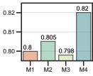
(a) Electronics

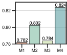
(b) Books

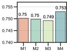
(c) Games

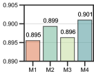
(d) Taobao

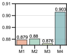
(e) MovieLens

Figure 4: Ablation Study On Public Datasets.

In this paper, the following models are selected to make comparisons with our proposed method, i.e., Meta-Wrapper:

• Base. This model uses the same Embedding+MLP architecture as the base predictor introduced in the preceding section, where the user interest is simply modeled as the sum of clicked-item embeddings. This model is selected as a baseline in many studies such as [4, 5, 66].

• Wide&Deep[32]. Wide&Deep model is widely accepted in real-world applications. It consists of two components: 1) wide module, which handles the manually designed features by a logistic regression model, 2) deep module, which is equivalent to the BaseModel. Following the practice in [2], we take a cross-product of all features as wide inputs.

• PNN[1]. PNN can be regarded as an improved version of BaseModel by adding a product layer after the embedding layer to model high-order feature interactions. It first inputs the feature embeddings into a dense layer and a product layer, then concatenates them together and uses other dense layers to get the output.

• DeepFM[2]. It takes factorization machines (FM) as a wide module in Wide&Deep to reduce the feature engineering efforts. It inputs feature embeddings into an FM and a deep component and then concatenates their outputs to the final output through a dense layer.

• DIN[4]. DIN applies the attention mechanism on top of the BaseModel for selecting relevant features in user’s behaviors. The attentive feature selector has the same architecture as ours introduced in the proceeding section.

• DIEN[5]. DIEN can be considered as an improved version of DIN. It uses GRU with an attentional updating gate to model the evolution of user interest.

• DMIN[66]. DMIN uses multi-head self-attention to model the interest evolution and extract multiple user interests within behavioral sequences. It is more efficient at inference stage compared with DIEN.

• xDeepFM[3]. xDeepFM uses Compressed Interaction Network (CIN) to model the feature crossing. This approach could describe high-order feature interactions in an explicit way.

• FGCNN[67]. FGCNN uses CNN to automatically generate new features, thereby augmenting feature space. This can be regarded as novel method to model the high-order feature-crossing.

• AutoFIS[68]. AutoFIS is proposed to automatically select feature interactions. In this paper, we use this strategy to select user behavioral features.

• AutoGroup[69] AutoGroup is also a feature selection based method. It first aggregates features into groups, and then applies feature selection on top of these groups. We also use this strategy to process user behavioral features in our experiments.

For all methods, two dense layers of the predictor are each with (80, 40) units. For DIN and our proposed method, the two dense layers in feature selector have 80 and 40 units, respectively. We adopt Mini-batch GD [61] as the optimizer for all methods, where the learning rate is dynamically scheduled by an exponential decay. Meanwhile, the number of epochs is set to 30. For fair comparison, the following hyperparameters are tuned by grid search: learning rate $\gamma$ in $\{1,0.1,0.01,0.0001,1.2,0.12,0.012,0.00012\}$; batch size in $\{32,64,128,256,512,1024\}$; weight decay rate in $\{0,1e-8,1e-7,1e-6,1e-5,1e-4\}$; embedding dimension in $\{32,48,64,96,128\}$. For Meta-Wrapper in Eq.(12), we additionally tune $\mu$ in $\{0.2,0.4,0.6,0.8\}$, $\beta$ in $\{0.0001,0.001,0.01,1\}$. Moreover, we set ${N}=1$ when comparing with other methods, but we tune ${N}$ in $\{1,2,3\}$ during the hyperparameter study.

6.1.3 Data Splitting

To simulate the experimental setting, we first sort the clicked records for each user by the timestamp and construct the training, validation and test set. Specifically, given ${T_{u}}$ behaviors for each user, we take last records as the positive samples in test set. From the rest records, we use the last one for each user as positive samples in validation set, while the remaining ones belong to the training set. For those methods needing out-of-bag data, we randomly split the training set into two parts at each epoch. Specifically, we regard $80\%$ of the samples as $\mathcal{D}^{(in)}$ in previous sections, while the rest $20\%$ of the samples are selected as $\mathcal{D}^{(out)}$. In each dataset, the items of positive samples are randomly replaced with another non-clicked item to construct the negative samples. In our experiment, each model is trained on the training set and its hyperparameters are tuned on the validation set. Notably, the validation set is not directly used to update parameters.

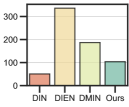
(a) Training Time on Electronics

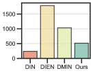
(b) Training Time on
Books

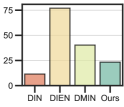
(c) Training Time on Games

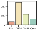
(d) Training Time on Taobao

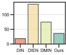
(e) Training Time on MovieLens

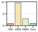
(f) Inference Time on Electronics

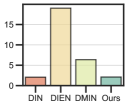
(g) Inference Time on
Books

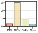
(h) Inference Time on Games

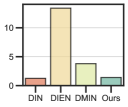
(i) Inference Time on Taobao

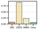
(j) Inference Time on MovieLens

Figure 5: Comparison of Training and Inference Time.

6.1.4 Evaluation Protocols

In the field of recommender systems, we often use AUC as the metric. It could evaluate the ranking order of all the items with an estimated click-through rate:

$$AUC=\frac{\sum_{b\in\mathcal{S}_{c}}{\texttt{rank}(b)}-\frac{{N_{c}}\times({N_{c}}+1)}{2}}{{N_{c}}\times{N_{u}}},$$ (19)

where $\mathcal{S}_{c}$ represents the set of all positive instances; $b$ denotes a positive instance drawn from $\mathcal{S}_{c}$; ${N_{c}}$ denotes the number of the positive (clicked) instances; ${N_{u}}$ is the number of the negative (unclicked) instances. Moreover, we also provide the relative improvement over the base model, following [70]. Since the AUC score of a random model is about 0.5, the relative improvement $Impr$ in this paper is defined as the following:

$$Impr=\left(\frac{AUC^{(model)}-0.5}{AUC^{(base)}-0.5}-1\right)\cdot 100\%,$$ (20)

where $AUC^{(model)}$ and $AUC^{(base)}$ refer to the AUC score w.r.t the measured model and base model, respectively.

6.2 Performance Comparison (RQ1)

Tab.I shows the performance of all competitors on five public datasets. From this table, we can get the following observations:

• All models with manual or automatic feature engineering outperform the base model significantly. This implies extensive feature engineering could improve the model performance on these datasets.

• Comparing the feature-crossing-based models, we see that the second-order feature-crossing methods (Wide&Deep, PNN, DeepFM) have better performance than their high-order counterparts (xDeepFM and FGCNN) in the vast majority of the cases. The reason might be that higher-order interactions are not suitable to model the behavioral features, though it is effective in dealing with general features.

• In most cases, general feature selection methods (AutoFIS and AutoGroup) are comparable with second-order feature-crossing methods, but have worse performance than attention-based methods (DIN, DIEN, DMIN). To see this, attention mechanism could select different historical behaviors with respect to different target items. On the contrary, general feature selection methods can only provide the same feature subsets for all target items, without considering the relevance between users’ past and present behaviors. These results also reflect the difference between user behavior features and general features.

• Meta-Wrapper achieves the best performance on all datasets. This implies that our meta-learned wrapping operator could enhance the learning of the feature selector (attentive module), thereby achieving better performance.

6.3 Ablation Study (RQ2)

To further justify our claim that improvements come from the meta-learned wrapping operator, we conduct a series of ablation experiments to validate the effectiveness of different modules of our method.

More specifically, we study the impact of adding the following components on top of a base model in the training process:

• C1: An attentive module as the user interest selector;

• C2: The first term of Eq.(17) as an auxiliary loss used to regularize the feature selector;

• C3: The wrapper method described in Example.(1) (i.e. GDmax-Wrapper) where we set inner-GD loops $N=1$;

• C4: The second term of Eq.(17) where we also set $N=1$ for fair comparisons.

Tab.III further shows which components are included in the different compared methods (M1-M4).

The experimental results are presented in Fig.4. From these results, we have the following observations:

• Comparing the performance of M1 and the base model, we can get that adding a feature selector (C1) on the top of the base predictor could significantly improve the model performance. Note that the performance can be found in the first row of Tab.I, which is not repeatedly shown in Fig.4.

• M2 brings an improvement on 4 out of 5 datasets with respect to M1. This illustrates that adding the first term of Eq.(17) (C2) actually works in CTR prediction tasks.

• M3 has lower performance than M2 on all datasets, which means that (C3) would result in performance degradation. The reason might be that inner parameters cannot be sufficiently trained when ${N}$ is small. Thus the inner solution is not precise enough to direct the outer-level problem, leading to the ineffectiveness of the wrapper method.

• M4 achieves the best performance on all datasets, which manifests the second term of Eq.(17) (C4) is also a source of performance improvements. This result is consistent with our theoretical analysis in Sec.(5.4).

TABLE III: Methods (M1-M4) w.r.t Components (C1-C4).

	C1	C2	C3	C4
M1	✓	$\times$	$\times$	$\times$
M2	✓	✓	$\times$	$\times$
M3	✓	✓	✓	$\times$
M4	✓	✓	✓	✓

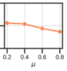
(a) $\mu$ w.r.t Electronics

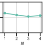
(b) $N$ w.r.t Electronics

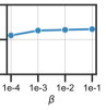
(c) $\beta$ w.r.t Electronics

(d) $\mu$ w.r.t Books

(e) $N$ w.r.t Books

(f) $\beta$ w.r.t Books

(g) $\mu$ w.r.t Games

(h) $N$ w.r.t Games

(i) $\beta$ w.r.t Games

(j) $\mu$ w.r.t Taobao

(k) $N$ w.r.t Taobao

(l) $\beta$ w.r.t Taobao

(m) $\mu$ w.r.t MovieLens

(n) $N$ w.r.t MovieLens

(o) $\beta$ w.r.t MovieLens

Figure 6: Hyperparameter Study on Public Datasets.

6.4 Generalization Performance (RQ3)

In this section, we conduct experiments on the synthetic data to demonstrate the overfitting in CTR prediction. We generate the synthetic data with user behavioral noises and observe to what extent are different models overfit. Meanwhile, we also show that Meta-Wrapper can better deal with such a situation.

6.4.1 Synthetic Data

We generate $100$ users and $10000$ items, while users and items are both divided into 10 groups. Here each group represents a type of interest. More specifically, the $i$-th user is assigned to the $g_{u}(i)$-th group, where $g_{u}(i)=(i\ MOD\ 10)$. Similarly, the $j$-th item is assigned to the $g_{i}(j)$-th group, where $g_{i}(j)=(j\ MOD\ 1000)$. For each user $i$, we select $50$ items as his/her interested items (i.e. positive instances), where the items are uniformly sampled from the subset $\{j|g_{i}(j)=g_{u}(i),j\in\mathcal{N},1\leq j\leq 10000\}$. Meanwhile, we uniformly sample $50$ non-interested items (i.e. negative instances) for each user $i$ from the item subset $\{j|g_{i}(j)\neq g_{u}(i),j\in\mathcal{N},1\leq j\leq 10000\}$. In this way, we can get a noiseless dataset with $5000$ positive instances and $5000$ negative instances. To simulate the noises, we now apply a perturbation to this dataset. More specifically, we generate labels $\bm{Y_{p}}$ for positive instances such that $\bm{Y_{p}}\sim Binomial(5000,0.5)$, and labels $\bm{Y_{n}}$ for negative instances such that $\bm{Y_{n}}\sim Binomial(5000,0.2)$. This implies that 1) there are about $50\%$ interested items labeled as non-clicked, and 2) about $20\%$ non-interested items labeled as clicked. In real-word scenario, it is possible that some interested items are ignored. Meanwhile, non-interested items might also be clicked by mistake. Thus we can say that such perturbations do exist in real-world CTR predictions, though it is not necessarily severe as our simulation. The reason why we construct such strong noises is to clearly show the overfitting and the improvements of Meta-Wrapper.

6.4.2 Experimental Results on Synthetic Data

Based on the synthetic data, we compare our proposed method with the 1) Base: the base model; 2) FS: the base model with attentive feature selector (FS); 3) FS+L2: the base model with FS and $L2$ weight decay ($L2$); 4) FS+DO: the base model with FS and $L2$ dropout (DO).

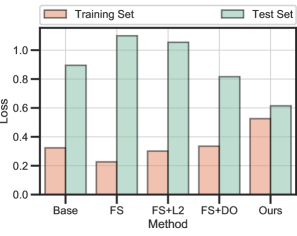
Figure 7: Overfitting on Synthetic Data With Strong Noises.

The experimental results are shown in Fig.7. For each approach, we can observe a major gap between the training and test loss, which results from our strong noises. Notably, the FS has lower training loss and higher test loss compared with Base. This means that attentive feature selector might exacerbate overfitting. Meanwhile, FS+L2 and FS+DO are a little better than FS, but its overfitting is still more serious than Base. This demonstrates the impact of $L2$ weight decay is limited in this scene. Finally, MW significantly reduces the training and test loss compared with other methods, where the overfitting is even less serious than Base.

From these results, we can conclude that 1) attentive feature selector would increase the overfitting risk, and 2) Meta-Wrapper is an effective approach to alleviate overfitting.

6.5 Efficiency Analysis (RQ4)

The data volume tends to be extremely large in practical applications, but the available computing resources are always limited. In such a scenario, a CTR prediction model should not only pay attention to the accuracy, but also consider the efficiency. Therefore, despite the effectiveness of Meta-Wrapper has been validated, it is also necessary to empirically analyse its computational efficiency.

In this section, we compare the training and inference time of Meta-Wrapper with three industrial models: DIN, DIEN and DMIN on one NVIDIA TITAN RTX GPU. In these experiments, we fix the inner loops $N=1$ for Meta-Wrapper. The experimental results are demonstrated in Fig.5. From this figure, we can observe that:

• At the training stage, DIN is the fastest approach. This result is in line with our expectation, since DIN is the most simple method compared with the other four competitors. Meanwhile, DIEN and DMIN need more training time, especially DIEN. This is because they have the complex modeling of sequential evolution. DMIN is faster than DIEN since it uses transformer instead of RNN to improve the concurrency. Moreover, the training time of Meta-Wrapper is about twice as DIN, which is consistent with our theoretical analysis.

• At the inference stage, DIEN is still the slowest method, and DMIN is a little faster than DIEN by virtue of its parallel computing capability. Meanwhile, DIN and Meta-Wrapper are significantly faster than others. Notably, our proposed meta-learning strategy only focuses on the training stage, so the inference time of Meta-wrapper should be equal to DIN. This is also proved by experimental results.

6.6 Hyperparameter Study (RQ5)

Recall that our final loss function Eq.(12) introduces three hyperparameters: 1) the weight of feature selection task $\mu$, 2) inner-level learning rate $\beta$ and 3) the number of inner-loops ${N}$. We study how these hyperparameters affect the model performance.

Fig.(6) presents our experimental results on five datasets, respectively. On Electronics dataset, all three hyperparameters do not have a great impact on performance. On Books, Games and Taobao, $\mu$ has a relatively larger impact on performance, while the impact of $\beta$ and ${N}$ is almost negligible. On MovieLens dataset, $\mu$, $\beta$ and ${N}$ all have an impact on performance, but the impact is quite small. Above all, the changing of performance is relatively evident when tuning the value of $\mu$, while it is quite stable across different $\beta$ and ${N}$. Therefore, we should give priority to tune the value of $\mu$ in practical applications, for the sake of better performance. Moreover, the stable performance w.r.t ${N}$ shows that Meta-Wrapper is robust towards the number of inner loops. In this way, the wrapper method could become computationally tractable by setting a smaller number of inner-loops ${N}$.

7 Conclusion

In this paper, we propose a differentiable wrapper method, namely Meta-Wrapper, to automatically select user interests in CTR prediction tasks. More specifically, we first regard user interest modeling as a feature selection problem. Then we provide the objective function, under the framework of the wrapper method, for such a problem. Moreover, we design a differentiable wrapping operator to simultaneously improve the efficiency and flexibility of the wrapper method. Based on these, the learning problems of the feature selector and downstream predictor are unified as a bilevel optimization which can be solved by a meta-learning algorithm. Meanwhile, we prove the effectiveness of our proposed method from a theoretical perspective. From the experimental results on three datasets, we also observe that our method significantly improves the performance of CTR prediction in recommender systems. In the future, we will try to incorporate more criteria besides performance into the framework of the differentiable wrapper to improve the user interest selection in CTR prediction.

Tianwei Cao received the M.E. degree in computer science and technology from University of Science and Technology Beijing (USTB) in 2017. He is currently pursuing the Ph.D. degree with University of Chinese Academy of Sciences. His research interests is data mining, especially recommender system and computational advertising.

Qianqian Xu received the B.S. degree in computer science from China University of Mining and Technology in 2007 and the Ph.D. degree in computer science from University of Chinese Academy of Sciences in 2013. She is currently an Associate Professor with the Institute of Computing Technology, Chinese Academy of Sciences, Beijing, China. Her research interests include statistical machine learning, with applications in multimedia and computer vision. She has authored or coauthored 40+ academic papers in prestigious international journals and conferences, including T-PAMI/IJCV/T-IP/T-KDE/ICML/NeurIPS/CVPR/AAAI, etc. She served as a reviewer for several top-tier journals and conferences, such as T-PAMI, ICML, NeurIPS, ICLR, CVPR, ECCV, AAAI, IJCAI, and ACM MM, etc.

Zhiyong Yang received the M.Sc. degree in computer science and technology from University of Science and Technology Beijing (USTB) in 2017, and the Ph.D. degree from University of Chinese Academy of Sciences (UCAS) in 2021. He is currently a postdoctoral research fellow with the University of Chinese Academy of Sciences. His research interests lie in machine learning and learning theory, with special focus on AUC optimization, meta-learning/multi-task learning, and learning theory for recommender systems. He has authored or coauthored 20+ academic papers in top-tier international conferences and journals including T-PAMI/ICML/NeurIPS/CVPR. He served as a reviewer for several top-tier journals and conferences such as T-PAMI, ICML, NeurIPS and ICLR.

Qingming Huang is a chair professor in the University of Chinese Academy of Sciences and an adjunct research professor in the Institute of Computing Technology, Chinese Academy of Sciences. He graduated with a Bachelor degree in Computer Science in 1988 and Ph.D. degree in Computer Engineering in 1994, both from Harbin Institute of Technology, China. His research areas include multimedia computing, image processing, computer vision and pattern recognition. He has authored or coauthored more than 400 academic papers in prestigious international journals and top-level international conferences. He is the associate editor of IEEE Trans. on CSVT and Acta Automatica Sinica, and the reviewer of various international journals including IEEE Trans. on PAMI, IEEE Trans. on Image Processing, IEEE Trans. on Multimedia, etc. He is a Fellow of IEEE and has served as general chair, program chair, track chair and TPC member for various conferences, including ACM Multimedia, CVPR, ICCV, ICME, ICMR, PCM, BigMM, PSIVT, etc.

[Convergence Result of Alg.3]

TABLE IV: Notations and Descreptions.

Notations	Descreptions
$N_{\theta}$, $N_{\phi}$	$N_{\theta}$ and $N_{\phi}$ are dimensions of parameters vector $\bm{\theta}$ and $\bm{\phi}$, and $p=N_{\theta}+N_{\phi}$;
$p$	The number of all parameters: $p=N_{\theta}+N_{\phi}$;
${\bm{\theta}},{\bm{\theta}_{w}},{\bm{\theta}_{u}}$	Parameters value of base predictor: ${\bm{\theta}},{\bm{\theta}_{w}},{\bm{\theta}_{u}}\in\mathbb{R}^{N_{\theta}}$;
${\bm{\phi}},{\bm{\phi}_{w}},{\bm{\phi}_{u}}$	Parameters value of feature selector: ${\bm{\theta}},{\bm{\phi}_{w}},{\bm{\phi}_{u}}\in\mathbb{R}^{N_{\phi}}$;
$\bm{z}$, $\bm{z}_{w}$, $\bm{z}_{u}$	All parameters: $\bm{z}=[\bm{\theta}^{\top},\bm{\phi}^{\top}]^{\top}\in\mathbb{R}^{p}$, $\bm{z}_{w}=[{\bm{\theta}^{\top}_{w}},{\bm{\phi}^{\top}_{q}}]^{\top}\in\mathbb{R}^{p}$, $\bm{z}_{u}=[{\bm{\theta}^{\top}_{u}},{\bm{\phi}^{\top}_{u}}]^{\top}\in\mathbb{R}^{p}$;
$\bm{\theta}^{(i)}(\bm{\phi})$	The value of $\bm{\theta}$ after $i$ loops of inner-GD;
$\bm{z}_{w}^{{(i})}$, $\bm{z}_{u}^{{(i})}$	Parameters value after $i$ loops of inner-GD: $\bm{z}_{w}^{{(i})}=[{(\bm{\theta}^{(i)}(\bm{\phi}_{w}))}^{\top},{\bm{\phi}_{w}}^{\top}]^{\top}$, $\bm{z}_{u}^{{(i})}=[{(\bm{\theta}^{(i)}(\bm{\phi}_{u}))}^{\top},{\bm{\phi}_{u}}^{\top}]^{\top}$;
$G_{w}^{(i,j)},G_{u}^{(i,j)}$	Gradient on $\mathcal{D}^{(in)}$ across inner-GD loops: $G_{w}^{(i,j)}=\nabla_{\bm{z}_{w}^{{(i})}}L^{(in)}(\bm{z}_{w}^{{(j})}),G_{u}^{(i,j)}=\nabla_{\bm{z}_{u}^{{(i})}}L^{(in)}(\bm{z}_{u}^{{(j})})$;
$\hat{G}_{w}^{(i,j)},\hat{G}_{u}^{(i,j)}$	Gradient on $\mathcal{D}^{(out)}$ across inner-GD loops: $G_{w}^{(i,j)}=\nabla_{\bm{z}_{w}^{{(i})}}L^{(out)}(\bm{z}_{w}^{{(j})}),G_{u}^{(i,j)}=\nabla_{\bm{z}_{u}^{{(i})}}L^{(out)}(\bm{z}_{u}^{{(j})})$;
$\mathcal{G}_{\square}$	The outer-level gradient: $\nabla_{\square}{\mathcal{L}(\bm{z})}$, where $\square\in\{\bm{z},\bm{\phi},\bm{\theta}\}$ and $\mathcal{L}$ is defined in Eq.(12);
$H_{w}^{(i)},H_{u}^{(i)}$	Hessian at $j$-th inner-GD step: $\nabla^{2}_{\bm{z}_{w}^{{(i})}}L^{(in)}(\bm{z}_{w}^{{(i})})^{\top}$, $\nabla^{2}_{\bm{z}_{u}^{{(i})}}L^{(in)}(\bm{z}_{u}^{{(i})})^{\top}$;
$\mathcal{T}$	Meta-learning Task: $\mathcal{T}_{i}=\{\mathcal{D}^{(in)}_{i},\mathcal{D}^{(out)}_{i}\}$, where subscript $i$ is the number of outer-GD step;
$\mathcal{P}(\mathcal{T})$	The distribution of $\mathcal{T}$;
$\bm{z}_{(i)}$	Parameters value after $i$ loops of Alg.3 (outer-GD).
$\mathcal{F}$	Expectated loss w.r.t $\mathcal{P}(\mathcal{T})$: $\mathbb{E}({\mathcal{L}(\bm{z})})$, ;
$\mathcal{F}_{i},\mathcal{F}(\bm{z}_{(i)})$	Expectated loss w.r.t $\mathcal{P}(\mathcal{T})$ at $i$-th outer-GD step: $\mathcal{F}_{i}=\mathcal{F}(\bm{z}_{(i)})=\mathbb{E}({\mathcal{L}(\bm{z}_{(i)})})$;

We start by proving the following lemmas. After that, we prove the convergence of Theorem.(1). The used notations are listed in Tab.IV.

Lemma 1.

Let $C_{3}=N\beta C_{2}(\sqrt{p}+\beta C_{1})^{{N}-1}C_{0}$ and $C_{L1}=2C_{1}+\mu C_{3}.$ Based on the notations defined in Tab.IV, for arbitrary parameters $\bm{z}_{w},\bm{z}_{u}\in\mathbb{R}^{p}$, we have

$$\|\nabla_{\bm{z}_{w}}\mathcal{F}-\nabla_{\bm{z}_{u}}\mathcal{F}\|\leq C_{L1}\|\bm{z}_{w}-\bm{z}_{u}\|.$$

Proof.

First, we have

$$\|\nabla_{\bm{z}}\mathcal{L}(\bm{\theta},\bm{\phi})\| \leq\|\nabla_{\bm{\theta}}\mathcal{L}(\bm{\theta},\bm{\phi})\|+\|\nabla_{\bm{\phi}}\mathcal{L}(\bm{\theta},\bm{\phi})\|.$$ (21)

Based on Eq.(12), we can get that

$$\nabla_{\bm{\theta}}\mathcal{L}(\bm{\theta},\bm{\phi}) =\nabla_{\bm{\theta}}L^{(in)}(\bm{\theta},\bm{\phi})$$ (22)

and

$$\nabla_{\bm{\phi}}\mathcal{L}(\bm{\theta},\bm{\phi}) =\nabla_{\bm{\phi}}L^{(in)}(\bm{\theta},\bm{\phi})+\mu\nabla_{\bm{\phi}}L^{(out)}(\bm{\theta}^{{(N)}},\bm{\phi}).$$ (23)

Thus we can derive that

$$\|\nabla_{\bm{z}_{w}}\mathcal{L}(\bm{\theta}_{w},\bm{\phi}_{w})-\nabla_{\bm{z}_{u}}\mathcal{L}(\bm{\theta}_{u},\bm{\phi}_{u})\|$$ (24)

$$\leq \|\nabla_{\bm{\theta}_{w}}L^{(in)}(\bm{\theta}_{w},\bm{\phi}_{w})-\nabla_{\bm{\theta}_{u}}L^{(in)}(\bm{\theta}_{u},\bm{\phi}_{u})\|$$

$$+\|\nabla_{\bm{\phi}_{w}}L^{(in)}(\bm{\theta}_{w},\bm{\phi}_{w})-\nabla_{\bm{\phi}_{u}}L^{(in)}(\bm{\theta}_{u},\bm{\phi}_{u})\|$$

$$+\mu\|\nabla_{\bm{\phi}_{w}}L^{(out)}({\bm{\theta}_{w}}^{{(N)}},\bm{\phi}_{w})-\nabla_{\bm{\phi}_{u}}L^{(out)}({\bm{\theta}_{u}}^{{(N)}},\bm{\phi}_{u})\|$$

$$\leq 2C_{1}\|\bm{z}_{w}-\bm{z}_{u}\|+\mu A_{0},$$

where we define

$$A_{0}=\|\nabla_{\bm{\phi}_{w}}L^{(out)}({\bm{\theta}_{w}}^{{(N)}},\bm{\phi}_{w})-\nabla_{\bm{\phi}_{u}}L^{(out)}({\bm{\theta}_{u}}^{{(N)}},\bm{\phi}_{u})\|.$$ (25)

Notably, ${\bm{\theta}_{w}}^{{(N)}}$ and ${\bm{\theta}_{u}}^{{(N)}}$ are functions of $\bm{\phi}_{w}$ and $\bm{\phi}_{u}$, respectively.

We next upper-bound $A$ in the above inequality. To this end, we first regard $L^{(out)}(\bm{\theta}^{{(N)}},\bm{\phi})$ as a special case of ${N}$-step MAML loss [59] where both $\bm{\theta}$ and $\bm{\phi}$ are meta-learned but with different learning rate. Specifically, we reformulate the inner-level learning rate as a vector $\bm{q}_{\beta}\in\mathbb{R}^{p}$ such that

$$\bm{q}_{\beta}[i]=\left\{\begin{array}[]{lr}\beta,\ \ i\leq{N_{\theta}};\\ 0,\ \ otherwise.\\ \end{array}\right.$$ (26)

This means that the inner learning rate for each parameter $i$ is $\bm{q}_{\beta}[i]$. Now the initial values $\bm{z}_{w}^{{(0)}}=\bm{z}$ are trainable parameters and $\bm{z}^{{(i+1})}=[{(\bm{\theta}^{(i+1)}(\bm{\phi}))}^{\top},{\bm{\phi}}^{\top}]^{\top}=\bm{z}^{{(i})}-\bm{q}_{\beta}\odot G_{w}^{(i,i)}$. Thus we can reformulate $A_{0}$ as following:

$$A_{0} =\|\nabla_{\bm{\phi}_{w}}L^{(out)}({\bm{\theta}_{w}}^{{(N)}},\bm{\phi}_{w})-\nabla_{\bm{\phi}_{u}}L^{(out)}({\bm{\theta}_{u}}^{{(N)}},\bm{\phi}_{u})\|$$ (27)

$$\leq\|\nabla_{\bm{z}}L^{(out)}(\bm{z}_{w}^{{(N})})-\nabla_{\bm{z}}L^{(out)}(\bm{z}_{u}^{{(N})})\|$$

$$=\|\hat{G}_{w}^{(0,{N})}-\hat{G}_{u}^{(0,{N}))}\|.$$

Then we come to the inner-GD rollouts. For each $0\leq j<{N}$, we have

$$\left\|\bm{z}_{w}^{{(j+1})}-\bm{z}_{u}^{{(j+1})}\right\|$$ (28)

$$= \left\|\bm{z}_{w}^{{(j})}-\bm{z}_{u}^{{(j})}-\bm{q}_{\beta}\odot\left(G_{w}^{(j,j)}-G_{u}^{(j,j)}\right)\right\|$$

$$\leq \left\|\bm{z}_{w}^{{(j})}-\bm{z}_{u}^{{(j})}\right\|+\left\|\bm{q}_{\beta}\odot\left(G_{w}^{(j,j)}-G_{u}^{(j,j)}\right)\right\|$$

$$\leq \left\|\bm{z}_{w}^{{(j})}-\bm{z}_{u}^{{(j})}\right\|+\left\|\beta\left(G_{w}^{(j,j)}-G_{u}^{(j,j)}\right)\right\|$$

$$= \left\|\bm{z}_{w}^{{(j})}-\bm{z}_{u}^{{(j})}\right\|+\beta\left\|G_{w}^{(j,j)}-G_{u}^{(j,j)}\right\|$$

$$= \left\|\bm{z}_{w}^{{(j})}-\bm{z}_{u}^{{(j})}\right\|+\beta C_{1}\left\|\bm{z}_{w}^{{(j})}-\bm{z}_{u}^{{(j})}\right\|$$

$$= (1+\beta C_{1})\left\|\bm{z}_{w}^{{(j})}-\bm{z}_{u}^{{(j})}\right\|$$

$$\cdots$$

$$\leq (1+\beta C_{1})^{j+1}\left\|\bm{z}_{w}^{{(0})}-\bm{z}_{u}^{{(0})}\right\|$$

$$\leq (\sqrt{p}+\beta C_{1})^{j+1}\left\|\bm{z}_{w}-\bm{z}_{u}\right\|.$$

From this, we can get the following inequality:

$$\left\|\nabla_{\bm{z}_{w}^{{(N})}}L^{(out)}(\bm{z}_{w}^{{(N})})-\nabla_{\bm{z}_{u}^{{(N})}}L^{(out)}(\bm{z}_{u}^{{(N})})\right\|$$ (29)

$$\leq C_{1}\left\|\bm{z}_{w}^{{(N})}-\bm{z}_{u}^{{(N})}\right\|$$

$$\leq C_{1}(\sqrt{p}+\beta C_{1})^{{N}}\left\|\bm{z}_{w}-\bm{z}_{u}\right\|.$$

Meanwhile, we have

$$\|\hat{G}_{w}^{(j,{N})}\|= \|(\prod_{i=j}^{{N-1}}(\bm{I}-\bm{q_{\beta}}\odot H_{w}^{(i)}))\hat{G}_{w}^{({N},{N})}\|$$ (30)

$$\leq (\prod_{i=j}^{{N-1}}\|\bm{I}-\bm{q_{\beta}}\odot H_{w}^{(i)}\|)\|\hat{G}_{w}^{({N},{N})}\|$$

$$\leq (\prod_{i=j}^{{N-1}}(\sqrt{p}+\|\beta H_{w}^{(i)}\|))\|\hat{G}_{w}^{({N},{N})}\|$$

$$\leq (\sqrt{p}+\beta C_{1})^{{N}-j}C_{0}$$

Furthermore, we introduce the following auxiliary notations for each $0\leq i<{N}$ and $0\leq j<{N}$:

$$A_{1}(j)=\hat{G}_{w}^{(j,N)}-\hat{G}_{u}^{(j,N)},$$ (31)

$$A_{2}(j)=H_{w}^{(j)}\hat{G}_{w}^{(j+1,N)}-H_{u}^{(j)}\hat{G}_{u}^{(j+1,N)},$$

$$A_{3}(j)=\left(H_{w}^{(j)}-H_{u}^{(j)}\right)\hat{G}_{u}^{(j+1,{N})},$$

$$A_{4}(j)=\beta C_{2}(\sqrt{p}+\beta C_{1})^{{N}-j-1}C_{0}.$$

Based on these, we can get the following inequality:

$$\|A_{1}(j)\|$$ (32)

$$= \left\|A_{1}(j+1)-\bm{q}_{\beta}\odot A_{2}(j)\right\|$$

$$= \|A_{1}(j+1)-\bm{q}_{\beta}\odot H_{w}^{(j)}A_{1}(j+1)-\bm{q}_{\beta}\odot A_{3}(j)\|$$

$$\leq \left\|A_{1}(j+1)\right\|+\beta\|H_{w}^{(j)}\|\left\|A_{1}(j+1)\right\|+\beta\left\|A_{3}(j)\right\|$$

$$\leq (\sqrt{p}+\beta C_{1})\left\|A_{1}(j+1)\right\|+A_{4}(j)\|\bm{z}_{w}^{{(j})}-\bm{z}_{u}^{{(j})}\|.$$

Thus the value of $A_{0}=\|A_{1}(0)\|$ can be obtained by applying the following chain of inequalities applies for each $0\leq j<N$:

$$A_{0}\leq (\sqrt{p}+\beta C_{1})\left\|A_{1}(1)\right\|+A_{4}(0)\|\bm{z}_{w}-\bm{z}_{u}\|$$ (33)

$$\leq (\sqrt{p}+\beta C_{1})^{2}\left\|A_{1}(2)\right\|$$

$$+\sum_{j=0}^{1}A_{4}(j)(\sqrt{p}+\beta C_{1})^{j}\|\bm{z}_{w}-\bm{z}_{u}\|$$

$$\cdots$$

$$\leq (\sqrt{p}+\beta C_{1})^{N}\left\|A_{1}(N)\right\|$$

$$+\sum_{j=0}^{N-1}A_{4}(j)(\sqrt{p}+\beta C_{1})^{j}\|\bm{z}_{w}-\bm{z}_{u}\|$$

$$\leq (\sqrt{p}+\beta C_{1})^{N}C_{1}\left\|\bm{z}_{w}-\bm{z}_{u}\right\|$$

$$+N\beta C_{2}(\sqrt{p}+\beta C_{1})^{{N}-1}C_{0}\|\bm{z}_{w}-\bm{z}_{u}\|$$

$$= C_{3}\left\|\bm{z}_{w}-\bm{z}_{u}\right\|.$$

Based on Eq.(33) and Eq.(24), we can get that

$$\|\nabla_{\bm{z}_{w}}\mathcal{F}-\nabla_{\bm{z}_{u}}\mathcal{F}\|$$ (34)

$$\leq \mathbb{E}(\|\nabla_{\bm{z}_{w}}\mathcal{L}(\bm{\theta}_{w},\bm{\phi}_{w})-\nabla_{\bm{z}_{u}}\mathcal{L}(\bm{\theta}_{u},\bm{\phi}_{u})\|)$$

$$\leq (2C_{1}+\mu C_{3})\left\|\bm{z}_{w}-\bm{z}_{u}\right\|$$

which is equivalent to the statement of this Lemma. ∎

Lemma 2.

Let $C_{L2}=C^{2}_{0}+\mu(\sqrt{p}+\beta C_{1})^{{2N}}C_{0}^{2}$. Based on the notations defined in Tab.IV, for arbitrary meta-model with parameters $\bm{\phi}\in\mathbb{R}^{{N_{\phi}}}$, the outer-level gradient $\mathcal{G}_{\bm{\phi}}$ holds that $\mathbb{E}\left(\|\mathcal{G}_{\bm{\phi}}\|^{2}\right)\leq C_{L2}$.

Proof.

According to Eq.(23), we can derive that

$$\|\mathcal{G}_{\bm{\phi}}\|^{2} \leq\|\nabla_{\bm{\phi}}L^{(in)}(\bm{\theta},\bm{\phi})\|^{2}+\mu\|\nabla_{\bm{\phi}}L^{(out)}(\bm{\theta}^{{(N)}},\bm{\phi})\|^{2}$$ (35)

$$\leq\|\nabla_{\bm{z}}L^{(in)}(\bm{z})\|^{2}+\mu\|\nabla_{\bm{z}}L^{(out)}(\bm{z}^{{(N)}})\|^{2}$$

$$\leq C^{2}_{0}+\mu\|\hat{G}_{w}^{(0,{N})}\|^{2}$$

Based on Eq.(30), we have

$$\|\hat{G}_{w}^{(0,{N})}\|^{2}\leq ((\sqrt{p}+\beta C_{1})^{{N}-j}C_{0})^{2}$$ (36)

$$= (\sqrt{p}+\beta C_{1})^{{2N}}C_{0}^{2}.$$

Now we can get that

$$\|\mathcal{G}_{\bm{\phi}}\| \leq C^{2}_{0}+\mu\|\hat{G}_{w}^{(0,{N})}\|$$ (37)

$$\leq C^{2}_{0}+\mu(\sqrt{p}+\beta C_{1})^{{2N}}C_{0}^{2}.$$

Thus the proof is is concluded. ∎

Lemma 3.

Let $C_{L3}=\frac{C_{L1}}{2}(C^{2}_{0}+C_{L2})$. Based on Lemma.(1) and Lemma.(2), as well as notations defined in Tab.IV, we have the following inequality for each $k\in\mathbb{N}$: $\sum_{i=1}^{k}\gamma_{i}\|\nabla_{\bm{z}}\mathcal{F}_{i-1}\|^{2}\leq\mathcal{F}_{0}+C_{L3}\sum_{i=1}^{k}\gamma_{i}^{2}.$

Proof.

For each $0<i\leq k$, we have

$$\|\nabla_{\bm{z}}\mathcal{F}_{i-1}\|^{2}\leq\|\nabla_{\bm{\theta}}\mathcal{F}_{i-1}\|^{2}+\|\nabla_{\bm{\phi}}\mathcal{F}_{i-1}\|^{2}.$$ (38)

So we can derive that

$$\sum_{i=1}^{k}\gamma_{i}\|\nabla_{\bm{z}}\mathcal{F}_{i-1}\|^{2}$$ (39)

$$\leq \sum_{i=1}^{k}\gamma_{i}(\|\nabla_{\bm{\theta}}\mathcal{F}_{i-1}\|^{2}+\|\nabla_{\bm{\phi}}\mathcal{F}_{i-1}\|^{2})$$

$$\leq \sum_{i=1}^{k}\gamma_{i}\|\nabla_{\bm{\theta}}\mathcal{F}_{i-1}\|^{2}+\sum_{i=1}^{k}\gamma_{i}\|\nabla_{\bm{\phi}}\mathcal{F}_{i-1}\|^{2}.$$

Based on Eq.(4.3) from [61], we have

$$\mathcal{F}_{i}\leq \mathcal{F}_{i-1}+\nabla_{\bm{\theta}}\mathcal{F}_{i-1}^{\top}(\bm{\theta}_{(i)}-\bm{\theta}_{(i-1)})+\frac{C_{L1}}{2}\|\bm{\theta}_{(i)}-\bm{\theta}_{(i-1)}\|^{2}$$ (40)

$$+\nabla_{\bm{\phi}}\mathcal{F}_{i-1}^{\top}(\bm{\phi}_{(i)}-\bm{\phi}_{(i-1)})+\frac{C_{L1}}{2}\|\bm{\phi}_{(i)}-\bm{\phi}_{(i-1)}\|^{2}$$

$$\leq \mathcal{F}_{i-1}-\gamma_{i}\nabla_{\bm{\theta}}\mathcal{F}_{i-1}^{\top}\mathcal{G}_{\bm{\theta}}+\frac{\gamma_{i}^{2}C_{L1}}{2}\|\mathcal{G}_{\bm{\theta}}\|^{2}$$

$$-\gamma_{i}\nabla_{\bm{\phi}}\mathcal{F}_{i-1}^{\top}\mathcal{G}_{\bm{\phi}}+\frac{\gamma_{i}^{2}C_{L1}}{2}\|\mathcal{G}_{\bm{\phi}}\|^{2}.$$

Taking the expectation over $\mathcal{P}(\mathcal{T})$ on both sides of the equation, we can get that

$$\mathcal{F}_{i}\leq \mathcal{F}_{i-1}-\gamma_{i}\nabla_{\bm{\theta}}\mathcal{F}_{i-1}^{\top}\mathbb{E}(\mathcal{G}_{\bm{\theta}})+\frac{\gamma_{i}^{2}C_{L1}}{2}\mathbb{E}(\|\mathcal{G}_{\bm{\theta}}\|^{2})$$ (41)

$$-\gamma_{i}\nabla_{\bm{\phi}}\mathcal{F}_{i-1}^{\top}\mathbb{E}(\mathcal{G}_{\bm{\phi}})+\frac{\gamma_{i}^{2}C_{L1}}{2}\mathbb{E}(\|\mathcal{G}_{\bm{\phi}}\|^{2})$$

$$\leq \mathcal{F}_{i-1}-\gamma_{i}\|\nabla_{\bm{\theta}}\mathcal{F}_{i-1}\|^{2}+\frac{\gamma_{i}^{2}C_{L1}}{2}\mathbb{E}(\|\mathcal{G}_{\bm{\theta}}\|^{2})$$

$$-\gamma_{i}\|\nabla_{\bm{\phi}}\mathcal{F}_{i-1}\|^{2}+\frac{\gamma_{i}^{2}C_{L1}}{2}\mathbb{E}(\|\mathcal{G}_{\bm{\phi}}\|^{2})$$

$$\leq \mathcal{F}_{i-1}-\gamma_{i}\|\nabla_{\bm{\theta}}\mathcal{F}_{i-1}\|^{2}+\frac{\gamma_{i}^{2}C_{L1}}{2}C^{2}_{0}$$

$$-\gamma_{i}\|\nabla_{\bm{\phi}}\mathcal{F}_{i-1}\|^{2}+\frac{\gamma_{i}^{2}C_{L1}}{2}C_{L2}.$$

This inequality is equivalent to

$$\gamma_{i}\|\nabla_{\bm{\theta}}\mathcal{F}_{i-1}\|^{2}+\gamma_{i}\|\nabla_{\bm{\phi}}\mathcal{F}_{i-1}\|^{2}$$ (42)

$$\leq \mathcal{F}_{i-1}-\mathcal{F}_{i}+\frac{\gamma_{i}^{2}C_{L1}}{2}(C^{2}_{0}+C_{L2}).$$

Summing up Eq.(42) for all $0<i\leq k$ yields that

$$\sum_{i=1}^{k}\gamma_{i}\|\nabla_{\bm{\theta}}\mathcal{F}_{i-1}\|^{2}+\sum_{i=1}^{k}\gamma_{i}\|\nabla_{\bm{\phi}}\mathcal{F}_{i-1}\|^{2}$$ (43)

$$\leq \mathcal{F}_{0}-\mathcal{F}_{k}+\sum_{i=1}^{k}\frac{\gamma_{i}^{2}C_{L1}}{2}(C^{2}_{0}+C_{L2}).$$

$$\leq \mathcal{F}_{0}+\sum_{i=1}^{k}\frac{\gamma_{i}^{2}C_{L1}}{2}(C^{2}_{0}+C_{L2}).$$

Thus we have

$$\sum_{i=1}^{k}\gamma_{i}\|\nabla_{\bm{z}}\mathcal{F}_{i-1}\|^{2}$$ (44)

$$\leq \sum_{i=1}^{k}\gamma_{i}\|\nabla_{\bm{\theta}}\mathcal{F}_{i-1}\|^{2}+\sum_{i=1}^{k}\gamma_{i}\|\nabla_{\bm{\phi}}\mathcal{F}_{i-1}\|^{2}$$

$$\leq \mathcal{F}_{0}+\sum_{i=1}^{k}\frac{\gamma_{i}^{2}C_{L1}}{2}(C^{2}_{0}+C_{L2}).$$

In this way, the proof is concluded. ∎

Proof of Theorem.(1).

Proof of Statement (1). Based on Eq.(40) and the result of Lemma.(2), we can get the following inequality by algebraic manipulation:

$$\mathcal{F}_{i-1}-\mathcal{F}_{i}> \gamma_{i}C^{2}_{0}+\gamma_{i}C_{L2}-\frac{\gamma_{i}^{2}}{2}C_{L3}.$$ (45)

From this, we can derive that when $\gamma_{i}<2\frac{C^{2}_{0}+C_{L2}}{C_{L3}}$, the right-side of Eq.(45) would be positive, thereby ensuring $\mathcal{F}_{i-1}>\mathcal{F}_{i}$. Thus the statement 1 is proved.

Proof of Statement (2). Since we have the condition that $\sum_{i=1}^{\infty}\gamma_{i}^{2}<\infty$, the right-hand side of the statement of Lemma.(3) converges to a finite value when $k\rightarrow\infty$. Thus the left-hand side is also convergent. Now suppose this statement is false. Then there exists $k_{0}\in\mathbb{N}$ and $B>0$ such that $\forall i\geq k_{0}:\|\nabla_{\bm{z}}\mathcal{F}_{i-1}\|^{2}>B$. However, for all $i>k_{0}$ we have

$$\sum_{i=1}^{k}\gamma_{i}\|\nabla_{\bm{z}}\mathcal{F}_{i-1}\|^{2}\geq B\sum_{i=k_{0}}^{k}\gamma_{i}\rightarrow\infty$$ (46)

while $k\rightarrow\infty$, which is a contradiction. Thus we can get that

$$\lim_{i\rightarrow\infty}{\|\nabla_{\bm{z}}\mathcal{F}_{i-1}\|^{2}}=0.$$ (47)

Taking a step further, the parameters $\bm{z}$ is bounded as $\|\bm{z}_{(i)}\|<C_{r}$. According to the Bolzano-Weierstrass theorem, any bounded sequence must have convergent subsequence, which immediately suggests the existence of at least one limit point for $\{\bm{z}_{(i)}\}_{i}$. Picking an arbitrary convergent subsequence $\{\bm{z}_{(s_{i})}\}_{i}$ with a limit point $\bm{z}^{\star}$. Since $s_{i}\rightarrow\infty$ when $i\rightarrow\infty$, we can get that

$$\lim_{i\rightarrow\infty}{\|\nabla_{\bm{z}}\mathcal{F}(\bm{z}_{(s_{i})})\|^{2}}=0$$ (48)

following the similar spirit of Eq.(47). Using the continuity of $\nabla_{\bm{z}}\mathcal{F}$, we have $\nabla_{\bm{z}}\mathcal{F}(\bm{z}_{(s_{i})})\rightarrow\nabla_{\bm{z}}\mathcal{F}(\bm{z}^{\star})$ when $i\rightarrow\infty$. Thus Eq.(48) is equivalent to ${\|\nabla_{\bm{z}}\mathcal{F}(\bm{z}^{\star})\|^{2}}=0$, which means that $\{\bm{z}_{(s_{i})}\}_{i}$ converges to a stationary point.

Proof of Statement (3). We have

$$\min_{0\leq j<k}\left(\|\nabla_{\bm{z}}\mathcal{F}_{j}\|^{2}\right)\sum_{i=1}^{k}\gamma_{i}\leq \sum_{i=1}^{k}\gamma_{i}\|\nabla_{\bm{z}}\mathcal{F}_{i-1}\|^{2}$$ (49)

$$\leq \mathcal{F}_{0}+C_{L3}\sum_{i=1}^{k}\gamma_{i}^{2}.$$

Dividing $\sum_{i=1}^{k}\gamma_{i}$ yields that

$$\min_{0\leq j<k}\|\nabla_{\bm{z}}\mathcal{F}_{j}\|^{2}\leq \frac{\mathcal{F}_{0}}{\sum_{i=1}^{k}\gamma_{i}}+C_{L3}\frac{\sum_{i=1}^{k}\gamma_{i}^{2}}{\sum_{i=1}^{k}\gamma_{i}}.$$ (50)

In this way, statement 3 is satisfied by observing that

$$\sum_{i=1}^{k}\gamma_{i}=\sum_{i=1}^{k}i^{-0.5}=\bm{\Omega}(k^{0.5}),$$ (51)

$$\sum_{i=1}^{k}\gamma_{i}^{2}=\sum_{i=1}^{k}i^{-1}=O(\log k)=\bm{\Omega}(k^{\epsilon})$$

for any $\epsilon>0$. ∎

References

- [1] Y. Qu, H. Cai, K. Ren, W. Zhang, Y. Yu, Y. Wen, and J. Wang, “Product-based neural networks for user response prediction,” in ICDM, 2016, pp. 1149–1154.
- [2] H. Guo, R. Tang, Y. Ye, Z. Li, and X. He, “Deepfm: A factorization-machine based neural network for CTR prediction,” in IJCAI, 2017, pp. 1725–1731.
- [3] J. Lian, X. Zhou, F. Zhang, Z. Chen, X. Xie, and G. Sun, “xdeepfm: Combining explicit and implicit feature interactions for recommender systems,” in SIGKDD, 2018, pp. 1754–1763.
- [4] G. Zhou, X. Zhu, C. Song, Y. Fan, H. Zhu, X. Ma, Y. Yan, J. Jin, H. Li, and K. Gai, “Deep interest network for click-through rate prediction,” in SIGKDD, 2018, pp. 1059–1068.
- [5] G. Zhou, N. Mou, Y. Fan, Q. Pi, W. Bian, C. Zhou, X. Zhu, and K. Gai, “Deep interest evolution network for click-through rate prediction,” in AAAI, 2019, pp. 5941–5948.
- [6] Y. Feng, F. Lv, W. Shen, M. Wang, F. Sun, Y. Zhu, and K. Yang, “Deep session interest network for click-through rate prediction,” in IJCAI, 2019, pp. 2301–2307.
- [7] K. Ren, J. Qin, Y. Fang, W. Zhang, L. Zheng, W. Bian, G. Zhou, J. Xu, Y. Yu, X. Zhu, and K. Gai, “Lifelong sequential modeling with personalized memorization for user response prediction,” in SIGIR, 2019, pp. 565–574.
- [8] Q. Pi, W. Bian, G. Zhou, X. Zhu, and K. Gai, “Practice on long sequential user behavior modeling for click-through rate prediction,” in SIGKDD, 2019, pp. 2671–2679.
- [9] J. Tang, S. Alelyani, and H. Liu, “Feature selection for classification: A review,” in Data Classification: Algorithms and Applications, 2014, pp. 37–64.
- [10] M. M. Kabir, M. M. Islam, and K. Murase, “A new wrapper feature selection approach using neural network,” Neurocomputing, vol. 73, no. 16-18, pp. 3273–3283, 2010.
- [11] L. Franceschi, P. Frasconi, S. Salzo, R. Grazzi, and M. Pontil, “Bilevel programming for hyperparameter optimization and meta-learning,” in ICML, 2018, pp. 1563–1572.
- [12] R. Vilalta and Y. Drissi, “A perspective view and survey of meta-learning,” Artificial intelligence review, vol. 18, no. 2, pp. 77–95, 2002.
- [13] H. B. McMahan, G. Holt, D. Sculley, M. Young, D. Ebner, J. Grady, L. Nie, T. Phillips, E. Davydov, D. Golovin, S. Chikkerur, D. Liu, M. Wattenberg, A. M. Hrafnkelsson, T. Boulos, and J. Kubica, “Ad click prediction: a view from the trenches,” in SIGKDD, 2013, pp. 1222–1230.
- [14] O. Chapelle, “Modeling delayed feedback in display advertising,” in SIGKDD, 2014, pp. 1097–1105.
- [15] M. Jahrer, A. Toscher, J.-Y. Lee, J. Deng, H. Zhang, and J. Spoelstra, “Ensemble of collaborative filtering and feature engineered models for click through rate prediction,” in KDDCup Workshop, 2012.
- [16] X. He, J. Pan, O. Jin, T. Xu, B. Liu, T. Xu, Y. Shi, A. Atallah, R. Herbrich, S. Bowers, and J. Q. Candela, “Practical lessons from predicting clicks on ads at facebook,” in ADKDD, 2014, pp. 5:1–5:9.
- [17] S. Rendle, Z. Gantner, C. Freudenthaler, and L. Schmidt-Thieme, “Fast context-aware recommendations with factorization machines,” in SIGIR, 2011, pp. 635–644.
- [18] X. Xin, B. Chen, X. He, D. Wang, Y. Ding, and J. Jose, “CFM: convolutional factorization machines for context-aware recommendation,” in IJCAI, 2019, pp. 3926–3932.
- [19] Y. Juan, D. Lefortier, and O. Chapelle, “Field-aware factorization machines in a real-world online advertising system,” in WWW, 2017, pp. 680–688.
- [20] J. Xiao, H. Ye, X. He, H. Zhang, F. Wu, and T. Chua, “Attentional factorization machines: Learning the weight of feature interactions via attention networks,” in IJCAI, 2017, pp. 3119–3125.
- [21] J. Pan, J. Xu, A. L. Ruiz, W. Zhao, S. Pan, Y. Sun, and Q. Lu, “Field-weighted factorization machines for click-through rate prediction in display advertising,” in WWW, 2018, pp. 1349–1357.
- [22] Y. Liu, X. Xia, L. Chen, X. He, C. Yang, and Z. Zheng, “Certifiable robustness to discrete adversarial perturbations for factorization machines,” in SIGIR. ACM, 2020, pp. 419–428.
- [23] M. Lin, S. Qiu, J. Ye, X. Song, Q. Qian, L. Sun, S. Zhu, and R. Jin, “Which factorization machine modeling is better: A theoretical answer with optimal guarantee,” in AAAI, 2019, pp. 4312–4319.
- [24] F. Hong, D. Huang, and G. Chen, “Interaction-aware factorization machines for recommender systems,” in AAAI, 2019, pp. 3804–3811.
- [25] L. Lan and Y. Geng, “Accurate and interpretable factorization machines,” in AAAI, 2019, pp. 4139–4146.
- [26] Y. Shan, T. R. Hoens, J. Jiao, H. Wang, D. Yu, and J. Mao, “Deep crossing: Web-scale modeling without manually crafted combinatorial features,” in SIGKDD, 2016, pp. 255–262.
- [27] K. He, X. Zhang, S. Ren, and J. Sun, “Deep residual learning for image recognition,” in CVPR, 2016, pp. 770–778.
- [28] W. Zhang, T. Du, and J. Wang, “Deep learning over multi-field categorical data - - A case study on user response prediction,” in ECIR, 2016, pp. 45–57.
- [29] X. He and T.-S. Chua, “Neural factorization machines for sparse predictive analytics,” in SIGIR, 2017, pp. 355–364.
- [30] W. Song, C. Shi, Z. Xiao, Z. Duan, Y. Xu, M. Zhang, and J. Tang, “Autoint: Automatic feature interaction learning via self-attentive neural networks,” in CIKM, 2019, pp. 1161–1170.
- [31] A. Vaswani, N. Shazeer, N. Parmar, J. Uszkoreit, L. Jones, A. N. Gomez, L. Kaiser, and I. Polosukhin, “Attention is all you need,” in NIPS, 2017, pp. 5998–6008.
- [32] H.-T. Cheng, L. Koc, J. Harmsen, T. Shaked, T. Chandra, H. Aradhye, G. Anderson, G. Corrado, W. Chai, M. Ispir et al., “Wide & deep learning for recommender systems,” in workshop on DLRS, 2016, pp. 7–10.
- [33] W. Liu, R. Tang, J. Li, J. Yu, H. Guo, X. He, and S. Zhang, “Field-aware probabilistic embedding neural network for CTR prediction,” in RecSys, 2018, pp. 412–416.
- [34] R. Wang, B. Fu, G. Fu, and M. Wang, “Deep & cross network for ad click predictions,” in ADKDD, 2017, 2017, pp. 12:1–12:7.
- [35] F. Feng, X. He, J. Tang, and T. Chua, “Graph adversarial training: Dynamically regularizing based on graph structure,” IEEE Trans. Knowl. Data Eng., 2020.
- [36] S. Li, W. Lei, Q. Wu, X. He, P. Jiang, and T. Chua, “Seamlessly unifying attributes and items: Conversational recommendation for cold-start users,” TOIS, 2021.
- [37] Y. Bengio, O. Delalleau, N. Roux, J.-F. Paiement, P. Vincent, and M. Ouimet, “Feature extraction: Foundations and applications, chapter spectral dimensionality reduction,” 2003.
- [38] J. Gui, Z. Sun, S. Ji, D. Tao, and T. Tan, “Feature selection based on structured sparsity: A comprehensive study,” TNNLS, vol. 28, no. 7, pp. 1490–1507, 2017.
- [39] R. Shumway, “Statistics and data analysis in geology,” 1987.
- [40] H. Peng, F. Long, and C. H. Q. Ding, “Feature selection based on mutual information: Criteria of max-dependency, max-relevance, and min-redundancy,” TPAMI, vol. 27, no. 8, pp. 1226–1238, 2005.
- [41] H. Liu, H. Mao, and Y. Fu, “Robust multi-view feature selection,” in ICDM, 2016, pp. 281–290.
- [42] R. O. Duda, P. E. Hart, and D. G. Stork, Pattern classification. John Wiley & Sons, 2012.
- [43] J. Liu, S. Ji, and J. Ye, “Multi-task feature learning via efficient l2, 1-norm minimization,” in UAI, 2009.
- [44] D. Ming, C. Ding, and F. Nie, “A probabilistic derivation of LASSO and l12-norm feature selections,” in AAAI, 2019, pp. 4586–4593.
- [45] D. Bahdanau, K. Cho, and Y. Bengio, “Neural machine translation by jointly learning to align and translate,” in ICLR, 2015.
- [46] R. B. Girshick, J. Donahue, T. Darrell, and J. Malik, “Rich feature hierarchies for accurate object detection and semantic segmentation,” in CVPR, 2014, pp. 580–587.
- [47] D. Erhan, C. Szegedy, A. Toshev, and D. Anguelov, “Scalable object detection using deep neural networks,” in CVPR, 2014, pp. 2155–2162.
- [48] M. Jaderberg, K. Simonyan, A. Zisserman, and K. Kavukcuoglu, “Spatial transformer networks,” in NIPS, 2015, pp. 2017–2025.
- [49] Z. Laskar and J. Kannala, “Context aware query image representation for particular object retrieval,” in SCIA, 2017, pp. 88–99.
- [50] L. Yao, A. Torabi, K. Cho, N. Ballas, C. J. Pal, H. Larochelle, and A. C. Courville, “Describing videos by exploiting temporal structure,” in ICCV, 2015, pp. 4507–4515.
- [51] F. Ma, R. Chitta, J. Zhou, Q. You, T. Sun, and J. Gao, “Dipole: Diagnosis prediction in healthcare via attention-based bidirectional recurrent neural networks,” in SIGKDD, 2017, pp. 1903–1911.
- [52] Y. Li, C. Chen, and W. W. Wasserman, “Deep feature selection: Theory and application to identify enhancers and promoters,” in RECOMB, 2015, pp. 205–217.
- [53] D. Roy, K. S. R. Murty, and C. K. Mohan, “Feature selection using deep neural networks,” in IJCNN, 2015, pp. 1–6.
- [54] Y. Koren, “Factorization meets the neighborhood: a multifaceted collaborative filtering model,” in SIGKDD, 2008, pp. 426–434.
- [55] X. He, L. Liao, H. Zhang, L. Nie, X. Hu, and T. Chua, “Neural collaborative filtering,” in WWW, 2017, pp. 173–182.
- [56] X. He, X. Du, X. Wang, F. Tian, J. Tang, and T. Chua, “Outer product-based neural collaborative filtering,” in IJCAI, 2018, pp. 2227–2233.
- [57] X. He, Z. He, J. Song, Z. Liu, Y. Jiang, and T. Chua, “NAIS: neural attentive item similarity model for recommendation,” IEEE Trans. Knowl. Data Eng., vol. 30, no. 12, pp. 2354–2366, 2018.
- [58] T. Lin, C. Jin, and M. I. Jordan, “On gradient descent ascent for nonconvex-concave minimax problems,” arXiv preprint arXiv:1906.00331, 2019.
- [59] C. Finn, P. Abbeel, and S. Levine, “Model-agnostic meta-learning for fast adaptation of deep networks,” in ICML, 2017, pp. 1126–1135.
- [60] D. Ha, A. M. Dai, and Q. V. Le, “Hypernetworks,” in ICLR, 2017.
- [61] L. Bottou, F. E. Curtis, and J. Nocedal, “Optimization methods for large-scale machine learning,” SIAM Rev., vol. 60, no. 2, pp. 223–311, 2018.
- [62] S. S. Girija, “Tensorflow: Large-scale machine learning on heterogeneous distributed systems,” Software available from tensorflow. org, 2016.
- [63] A. Paszke, S. Gross, S. Chintala, G. Chanan, E. Yang, Z. DeVito, Z. Lin, A. Desmaison, L. Antiga, and A. Lerer, “Automatic differentiation in pytorch,” 2017.
- [64] A. Griewank and A. Walther, Evaluating derivatives: principles and techniques of algorithmic differentiation. SIAM, 2008.
- [65] B. Christianson, “Automatic hessians by reverse accumulation,” IMA Journal of Numerical Analysis, 1992.
- [66] Z. Xiao, L. Yang, W. Jiang, Y. Wei, Y. Hu, and H. Wang, “Deep multi-interest network for click-through rate prediction,” in CIKM. ACM, 2020, pp. 2265–2268.
- [67] B. Liu, R. Tang, Y. Chen, J. Yu, H. Guo, and Y. Zhang, “Feature generation by convolutional neural network for click-through rate prediction,” in WWW, 2019, pp. 1119–1129.
- [68] B. Liu, C. Zhu, G. Li, W. Zhang, J. Lai, R. Tang, X. He, Z. Li, and Y. Yu, “Autofis: Automatic feature interaction selection in factorization models for click-through rate prediction,” in SIGKDD, 2020, pp. 2636–2645.
- [69] B. Liu, N. Xue, H. Guo, R. Tang, S. Zafeiriou, X. He, and Z. Li, “Autogroup: Automatic feature grouping for modelling explicit high-order feature interactions in CTR prediction,” in SIGIR, 2020, pp. 199–208.
- [70] L. Yan, W. Li, G. Xue, and D. Han, “Coupled group lasso for web-scale CTR prediction in display advertising,” in ICML, 2014, pp. 802–810.