Anomalous Higgs boson couplings in weak boson fusion production at NNLO in QCD

Abstract

The production of Higgs bosons in weak boson fusion has the second largest cross section among Higgs-production processes at the LHC. As such, this process plays an important role in detailed studies of Higgs interactions with vector bosons. In this paper we extend the available description of Higgs boson production in weak boson fusion by considering anomalous $HVV$ interactions and NNLO QCD radiative corrections at the same time. We find that, while leading order QCD predictions are too uncertain to allow for detailed studies of the anomalous couplings, NLO QCD results are sufficiently precise, most of the time. The NNLO QCD corrections alter the NLO QCD predictions only marginally, but their availability enhances the credibility of conclusions based on NLO QCD computations.

I Introduction

The discovery of the Higgs boson nearly ten years ago completed the Standard Model (SM) of particle physics, providing, for the first time, experimental support for the hypothesis that electroweak symmetry is broken by a scalar field. By now quantum numbers of the discovered Higgs boson, as well as its couplings to gauge and matter fields, have been studied in great detail and it appears that the properties of the Higgs boson are closely aligned with the SM expectations. For example, the Higgs couplings to massive electroweak vector bosons have been measured to within ${\cal O}(30)$ percent of their Standard Model values (see e.g. Refs Aad et al. (2020); Sirunyan et al. (2021)).

Verifying the Higgs boson couplings to a better, perhaps a few percent, precision is the goal of the LHC Run III and, especially, of the high-luminosity LHC. Reaching this goal will not be easy as it will require combining precise measurements with very detailed theoretical predictions. In addition, assuming that deviations in Higgs couplings are found, understanding their origin and what they imply becomes important. A convenient way to investigate this in a relatively model-independent way is to use an Effective Field Theory (EFT) framework and parameterize deviations from the Standard Model by higher-dimensional operators that depend on the Standard Model fields. These operators modify interactions between Standard Model particles and affect production cross sections and kinematic distributions that are observed at the LHC. An EFT that extends the SM is known as SMEFT Buchmuller and Wyler (1986); Grzadkowski et al. (2010); Brivio and Trott (2019).

Assuming that SMEFT provides a faithful description of beyond the Standard Model (BSM) physics, it becomes important to extract Wilson coefficients of higher-dimensional operators from the experimental data. Similar to measurements of Standard Model parameters, such an extraction of Wilson coefficients is affected by radiative corrections, of which QCD corrections are especially important. In this paper we investigate the interplay between anomalous couplings and radiative corrections for Higgs production in weak boson fusion (WBF). Such an interplay can be quite subtle for this process. Indeed, corrections to inclusive Higgs production in WBF are known to be small, but their impact on kinematic distributions can be larger. Anomalous couplings also distort kinematic distributions and, in fact, it is known that shapes of various observables often provide the best means to distinguish between different anomalous couplings (see e.g. Refs Plehn et al. (2002); Figy and Zeppenfeld (2004); Hankele et al. (2006)). Hence, for a reliable EFT analysis it becomes important to understand to what extent the effects of anomalous couplings and QCD corrections can be disentangled.

The theoretical description of Higgs production in weak boson fusion is very advanced. At the inclusive level, N³LO QCD corrections are known in the so-called factorized approximation Dreyer and Karlberg (2016). At the differential level, factorized NNLO QCD corrections  Cacciari et al. (2015); Cruz-Martinez et al. (2018); Asteriadis et al. (2022) as well as NLO EW corrections Ciccolini et al. (2007, 2008); Figy et al. (2012) are available. The dominant non-factorizable corrections have been studied in Refs Bolzoni et al. (2010, 2012); Liu et al. (2019); Dreyer et al. (2020). Theoretical predictions that include the anomalous couplings together with the NLO corrections to Higgs boson production in weak boson fusion can be obtained using such programs as HAWK Denner et al. (2015), VBFNLO Hankele et al. (2006); Baglio et al. (2014) and Madgraph5 Alwall et al. (2011).

In this paper we extend these results by computing NNLO QCD corrections to weak boson fusion in the factorized approximation in the presence of anomalous $HVV$ couplings. Although the $HVV$ vertex is not affected by QCD effects, such a computation is non-trivial since obtaining fully-differential predictions for the WBF process with NNLO QCD accuracy Cacciari et al. (2015); Cruz-Martinez et al. (2018); Asteriadis et al. (2022) is quite demanding. The reason behind this is the relative smallness of radiative corrections and a very large phase space (typical for a $2\to 5$ process) whose efficient generation is challenging.

In this paper, we employ the calculation of NNLO QCD corrections reported in Ref. Asteriadis et al. (2022). It is performed using the nested soft-collinear subtraction scheme Caola et al. (2017) which was adapted to WBF kinematics in Ref. Asteriadis et al. (2020). It provides a sufficiently efficient implementation and phase-space sampling that allowed us to incorporate decays of the Higgs boson Asteriadis et al. (2022) into the calculation. This efficiency is quite important for studying the anomalous couplings, especially for performing scans in the parameter space.

The rest of the paper is organized as follows. In Section II we describe the EFT framework which we employed in the calculations reported in this paper, and discuss the parametrization of the anomalous couplings adopted for this analysis. In Section III we present phenomenological results for the 13 TeV LHC. After describing our setup, we show predictions for cross sections and scans in the space of the anomalous couplings. We then focus on two scenarios where anomalous interactions are present but fiducial cross sections are indistinguishable from their Standard Model values. We then consider kinematic distributions which are sensitive to the anomalous couplings of the Higgs boson, and discuss the impact of higher order QCD corrections to them. We conclude in Section IV.

II Anomalous HVV interactions

For our analysis, we focus on anomalous $HVV$ interactions, where $V$ is a massive vector boson. Lorentz invariance and Bose symmetry imply that the most generic $HVV$ vertex must have the form

$$\begin{split}\vbox{\hbox{\includegraphics[scale={0.39}]{figs/hvv_vertex.pdf}}}&=\hskip 5.0pti\Big{[}g^{\mu\nu}A(p_{1}^{2},p_{2}^{2},p_{1}\cdot p_{2})\\[-16.0pt] &+p_{1}^{\nu}p_{2}^{\mu}\;B(p_{1}^{2},p_{2}^{2},p_{1}\cdot p_{2})\\ &+i\epsilon^{\mu\nu\rho\sigma}p_{1,\rho}p_{2,\sigma}\;C(p_{1}^{2},p_{2}^{2},p_{1}\cdot p_{2})\Big{]}\,,\end{split}$$ (1)

where $A$,$B$ and $C$ are arbitrary functions which, in the context of an effective theory, are Taylor-expandable in $p_{i}^{2}$ and $p_{i}\cdot p_{j}$ ($i,j=1,2$). It turns out that the dependence on these kinematic invariants can be further restricted. This point has been studied quite recently through an all-order EFT expansion in the context of the Standard Model Effective Theory Helset et al. (2020). In case of the dominant dimension-six operators, it has been shown Helset et al. (2020) that the functions $A$,$B$ and $C$ can be written as follows

$$\begin{split}A&=g_{HVV}^{(SM)}+g_{HVV}^{(3)}+g^{(1)}_{HVV}\frac{p_{1}\cdot p_{2}}{\Lambda^{2}}\,,\\ B&=-\frac{g^{(1)}_{HVV}}{\Lambda^{2}}\,,\qquad C=\frac{i\tilde{g}_{HVV}}{\Lambda^{2}}\,,\end{split}$$ (2)

where $\Lambda$ is the EFT scale and $g_{HVV}^{(i)}$ are $p_{1,2}$-independent constants. In Eq. (2), $g_{HVV}^{(SM)}$ is the Standard Model coupling, i.e. $g_{HWW}^{(SM)}=g\,m_{W}$ and $g_{HZZ}^{(SM)}=g\,m_{Z}/\cos\theta_{W}$, where $g$ is the weak coupling and $\theta_{W}$ is the weak mixing angle.

We find it convenient to parametrize the anomalous couplings as follows

$$\begin{split}&\frac{g^{(1)}_{HVV}}{g^{(SM)}_{HVV}}=2c^{(1)}_{HVV}\,,\qquad\frac{\tilde{g}_{HVV}}{g_{HVV}^{(SM)}}=6\pi\tilde{c}_{HVV}\,,\\ &\frac{g^{(3)}_{HVV}}{g_{HVV}^{(SM)}}+\frac{m_{H}^{2}}{\Lambda^{2}}\frac{g^{(1)}_{HVV}}{g^{(SM)}_{HVV}}=\frac{m_{H}^{2}}{\Lambda^{2}}c^{(2)}_{HVV}\,.\end{split}$$ (3)

The new constants $c_{HVV}^{(i)}$ are dimensionless; in terms of these constants, the coupling of the Higgs boson and the electroweak vector bosons reads, c.f. Eq. (1),

$$\begin{split}\vbox{\hbox{\includegraphics[scale={0.39}]{figs/hvv_vertex.pdf}}}&=\hskip 5.0ptig_{HVV}^{(SM)}\bigg{[}g^{\mu\nu}\bigg{(}1+\frac{m_{H}^{2}}{{\Lambda}^{2}}\ c_{HVV}^{(2)}\\[-12.0pt] &\hphantom{{}={}}+\frac{p_{1}^{2}+p_{2}^{2}}{{\Lambda}^{2}}\ c_{HVV}^{(1)}\bigg{)}+\frac{2p_{1}^{\nu}p_{2}^{\mu}}{{\Lambda}^{2}}c_{HVV}^{(1)}\end{split}$$

$$-\tilde{c}_{HVV}(6\pi)\epsilon^{\mu\nu\rho\sigma}\frac{p_{1,\rho}p_{2,\sigma}}{{\Lambda}^{2}}\bigg{]}\,.$$ (4)

The factor $(6\pi)$ introduced in the $CP$-odd term is chosen for convenience; indeed, as we will see later, with this normalization and for $\Lambda=1\leavevmode\nobreak\ {\rm TeV}$, $\tilde{c}_{HVV}\sim 1$ induces ${\mathcal{O}}(1\%)$ corrections to the fiducial cross section.

In general, the $HZZ$ and $HWW$ anomalous couplings do not have to be the same. However, for simplicity, in the analysis below we will assume that, by factorizing the SM couplings, we already account for main differences between them. Hence, in what follows, we restrict ourselves to the case where $c_{HZZ}^{(1,2)}=c_{HWW}^{(1,2)}=c_{HVV}^{(1,2)}$ and $\tilde{c}_{HZZ}=\tilde{c}_{HWW}=\tilde{c}_{HVV}$.

III Results at the 13 TeV LHC

Setup

For the phenomenological results reported in this paper, we use the same parameters and kinematic selection criteria as in Ref. Asteriadis et al. (2020). We collect them here for completeness. We consider proton-proton collisions with the center-of-mass energy 13 TeV and treat the Higgs boson as stable. We use the Higgs mass $m_{H}=125\leavevmode\nobreak\ {\rm GeV}$, the vector boson masses $M_{W}=80.398\leavevmode\nobreak\ {\rm GeV}$ and $M_{Z}=91.1876\leavevmode\nobreak\ {\rm GeV}$, and their widths $\Gamma_{W}=2.105\leavevmode\nobreak\ {\rm GeV}$ and $\Gamma_{Z}=2.4952\leavevmode\nobreak\ {\rm GeV}$. We use the Fermi constant $G_{F}=1.16639\times 10^{-5}{\rm GeV}^{-2}$ to derive the weak couplings and we set the CKM matrix to an identity matrix. We employ the NNPDF31-nnlo-as-118 parton distribution functions Ball et al. (2017) and use them for all calculations reported in this paper irrespective of the nominal perturbative order. We also use $\alpha_{s}(M_{Z})=0.118$. The evolution of the parton distribution functions and the strong coupling constant is obtained from LHAPDF Buckley et al. (2015). Finally, we employ dynamical renormalization and factorization scales $\mu_{R}=\mu_{F}=\mu$ using a central value Cacciari et al. (2015)

$$\mu_{0}=\sqrt{\frac{m_{H}}{2}\sqrt{\frac{m_{H}^{2}}{4}+p_{\perp,H}^{2}}}\,.$$ (5)

To define the weak boson fusion fiducial volume we reconstruct jets using the inclusive anti-$k_{\perp}$ algorithm Cacciari et al. (2008) with $R=0.4$. We require events to contain at least two jets with transverse momenta $p_{\perp,j}>25\leavevmode\nobreak\ {\rm GeV}$ and rapidities $|y_{j}|<4.5$. Also, the two leading-$p_{\perp}$ jets should be separated by a large rapidity interval $|y_{j_{1}}-y_{j_{2}}|>4.5$ and their invariant mass should be larger than $600\leavevmode\nobreak\ {\rm GeV}$. In addition, the two leading jets should be in different hemispheres in the laboratory frame; to enforce this, we require that the product of their rapidities in the laboratory frame is negative, $y_{j_{1}}y_{j_{2}}<0$. Finally, for definiteness we set $\Lambda=1\leavevmode\nobreak\ {\rm TeV}$ in all computations that we report below.

Fiducial cross sections

$\sigma_{\rm fid}$ (fb)	LO	NLO	NNLO
$X_{1}$	$971_{+69}^{-61}$	$890_{-18}^{+8}$	$859_{-10}^{+8}$
$X_{2}$	$0.413_{+0.039}^{-0.033}$	$0.398_{-0.005}^{-0.001}$	$0.383_{-0.005}^{+0.004}$
$X_{3}$	$19.57_{+2.22}^{-1.84}$	$19.64_{-0.07}^{-0.25}$	$19.25_{-0.18}^{+0.08}$
$X_{4}$	$26.43_{+1.80}^{-1.61}$	$23.45_{-0.66}^{+0.35}$	$22.53_{-0.42}^{+0.39}$

Table 1: Fiducial cross sections, in fb, at various orders of perturbative QCD using $\mu=\mu_{0}$. The sub- and super-scripts indicate the results computed with $\mu=\mu_{0}/2$ and $\mu=2\mu_{0}$, respectively. Numerical uncertainties are much smaller than scale uncertainties and are not shown. See text for further details.

We now present our results for the cross sections for Higgs production in weak boson fusion in the fiducial region described above, through NNLO QCD. Since three independent couplings appear in the $HVV$ vertex, cf. Eq. (II), the cross section naturally separates into six terms

$$\begin{split}\sigma_{\rm fid}&=\left(1+\frac{m_{H}^{2}}{{\Lambda}^{2}}{c_{HVV}^{(2)}}\right)^{2}X_{1}+\left({c_{HVV}^{(1)}}\right)^{2}X_{2}\\ &+\left({\tilde{c}^{\vphantom{(1)}}_{HVV}}\right)^{2}X_{3}+\left(1+\frac{m_{H}^{2}}{{\Lambda}^{2}}{c_{HVV}^{(2)}}\right){c_{HVV}^{(1)}}X_{4}\\ &+\left(1+\frac{m_{H}^{2}}{{\Lambda}^{2}}{c_{HVV}^{(2)}}\right){\tilde{c}^{\vphantom{(1)}}_{HVV}}X_{5}+\tilde{c}_{HVV}^{(1)}{\tilde{c}^{\vphantom{(1)}}_{HVV}}X_{6}\,.\end{split}$$ (6)

We note that $X_{1}$ is the Standard Model cross section. Two of the other terms, $X_{5,6}$ describe the interference of $CP$-even and $CP$-odd couplings and hence vanish for the azimuthally-symmetric cuts that we employ for computing fiducial cross sections. The results for the non-vanishing coefficients at leading, next-to-leading and next-to-next-to-leading orders are shown in Table 1.

We note that the radiative corrections to the various cross sections $X_{1,2,3,4}$ are similar but not identical. In general, when moving from LO to NLO we also observe a significant reduction in the dependence of the cross sections $X_{1,2,3,4}$ on the renormalization and factorization scales, which we estimate by changing the central scale $\mu_{0}$ in Eq. (5) by a factor two in either direction. Instead, there is no substantial scale-uncertainty reduction when moving from NLO to NNLO, and the NLO scale variation bands do not contain the NNLO result. This feature is well-known for the SM case, where it is also known that the NNLO and N³LO scale variation bands of the inclusive cross section do overlap Dreyer and Karlberg (2016). Because of this, it is understood in the context of SM studies that drawing conclusions based only on NLO QCD predictions and their scale uncertainty is delicate, while NNLO analyses should be more robust. Table 1 suggests that this also holds in the presence of anomalous $HVV$ interactions. These features will play an important role in the discussion below.

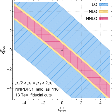
Figure 1: Allowed combinations of anomalous couplings $c^{(1)}_{HVV}$ and $c^{(2)}_{HVV}$ where the residual scale uncertainty band overlaps with SM prediction at the 13 TeV LHC. The color coding describes LO (hashed blue), NLO (yellow) and NNLO (squared red) calculations. The SM result is shown as black cross. See text for details.

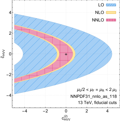
Figure 2: Same as Fig. 1 but for combinations involving the CP-odd anomalous coupling $\tilde{c}_{HVV}$. See text for details.

To illustrate the importance of higher order corrections, we now study the dependence of fiducial cross sections on the anomalous coupling constants at different orders of QCD perturbation theory. To this end, we take the Standard Model cross section as a reference point. We then consider a hypothetical BSM scenario with nonzero anomalous couplings, and declare it to be compatible with the Standard Model if the scale variation bands of the SM and BSM predictions overlap at a given order in QCD.

We show the results of this analysis in Figs 1,2 where different pairs of the anomalous couplings are chosen for two-dimensional projections. In those figures, the colored regions represent the allowed values for anomalous couplings according to the criterion just explained. We note that for this analysis we take Eq. (6) exactly as written, i.e. we include the contribution of dimension-six operators squared. One may worry about the consistency of this approach since we are neglecting the contribution of dimension-eight operators when defining the anomalous couplings. While this worry is clearly justified, the goal of our analysis is to study the possible interplay between higher order QCD corrections and EFT effects, and for this dealing with a representative set of anomalous couplings is sufficient. We stress however that the results of Table 1 make it straightforward for anyone to repeat the analysis including only the interference of dimension-six and SM operators. Similarly, it is immediate to change the definition of compatibility between SM and BSM predictions.

Having clarified our procedure, we now comment on the results, c.f. Figs 1,2. We note that since the cross sections $X_{2,3,4}$ describing the contributions of the anomalous couplings change the Standard Model cross section by about $2-3$ percent and the scale uncertainty of the leading order Standard Model cross section is about $10$ percent, only relatively large anomalous couplings can be excluded at leading order. The situation changes dramatically at NLO since theoretical uncertainties are reduced to about $1-2$ percent. There are further improvements at NNLO but they are minor; such improvements would imply changes in the anomalous couplings at the level of $\delta c_{HVV}^{(1,2)}\sim 0.1$ which, depending on the value of $c_{HVV}$ can be about ten percent. However, as we noted above, the NNLO shifts in the cross sections shown in Table 1 are often outside the NLO scale uncertainty bands. We then take the consistency of the NLO and NNLO results as an indicator of the reliability of the NLO analysis.

It is clear that the above study can be made more complex by, for example, considering three couplings at the same time, or by comparing results that include the contribution of dimension-six operators squared and results that do not, or by defining a more refined estimate of the compatibility of SM and BSM results. We do not pursue these investigations in this paper but we point out that once the fiducial cross sections $X_{1,2,3,4}$ are known, defining selection criteria and scanning the parameter space become straightforward. Obviously, if the fiducial cuts are to be changed, then all the cross sections $X_{1,2,3,4}$ have to be recalculated. We note in this respect that it takes about $25\,000$ CPU hours to compute each $X_{i}$ with good precision. Hence, if ${\cal O}(1000)$ CPU’s are available, about a few days of running is required.

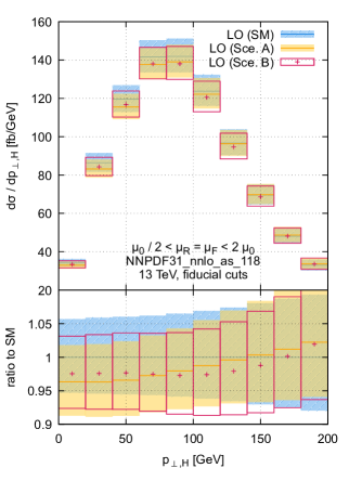
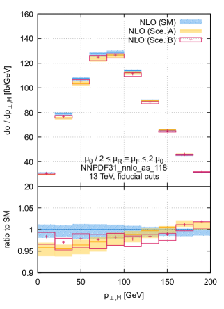
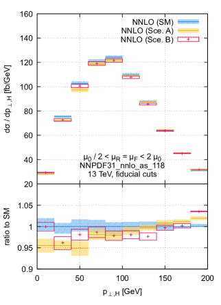
Figure 3: Transverse momentum distributions of the Higgs boson for LO (left), NLO (middle) and NNLO (right) QCD predictions. For each plot, the upper pane displays the SM (hashed blue), scenario A (solid yellow) and scenario B (red boxes) results as defined in the main text. The lower pane shows the ratio of these results to the SM result at central scale. The lines indicate the central renormalization and factorization scale choice, and the bands indicate the envelope of the results at different scales. See text for details.

Kinematic distributions

In the previous section, we discussed fiducial cross sections. This, of course, does not exhaust all opportunities for the analysis as kinematic distributions can also help to distinguish between the different couplings. To illustrate this point and to show how higher-order QCD corrections impact such an analysis, we consider two sets of anomalous couplings which lead to nearly identical cross sections. We choose the following scenarios

Sce. A: $$c_{HVV}^{(1)} =+1.5\,, \ \ c_{HVV}^{(2)} =-1.9\,, \ \ \tilde{c}_{HVV} =+0.6\,;$$

Sce. B: $$c_{HVV}^{(1)} =-1.8\,, \ \ c_{HVV}^{(2)} =-0.1\,, \ \ \tilde{c}_{HVV} =-1.5\,.$$

The results for fiducial cross sections at various orders of QCD perturbation theory are shown in Table 2. It is clear that, at leading order, the two scenarios cannot be distinguished from each other and from the Standard Model. Even with the significant reduction of scale variation uncertainties at next-to-leading and next-to-next-to-leading orders, the fiducial cross sections remain compatible.

$\sigma_{\textrm{fid}}$ (fb)	SM	Sce. A	Sce. B
LO	$971^{-61}_{+69}$	$960^{-61}_{+68}$	$965^{-63}_{+71}$
NLO	$890^{+8}_{-18}$	$882^{+7}_{-17}$	$890^{+6}_{-17}$
NNLO	$859^{+8}_{-10}$	$851^{+9}_{-8}$	$860^{+8}_{-8}$

Table 2: Central values of fiducial cross sections for the Standard Model and Scenarios A and B using $\mu=\mu_{0}$. The sub- and super-scripts indicate the results computed with $\mu=\mu_{0}/2$ and $\mu=2\mu_{0}$, respectively. Numerical uncertainties are much smaller than scale uncertainties and are not shown.

To understand if the two scenarios and the Standard Model can still be distinguished from each other, we consider the kinematic distributions. For most observables, however, there is very little difference between the various scenarios even at higher orders. To give an example, in Fig. 3 we consider the Higgs transverse momentum distribution. We report predictions at LO (left), NLO (middle) and NNLO (right), for the scenarios A and B and the SM. It is clear from this figure that one cannot disentangle the different models using LO predictions. At NLO and NNLO one starts seeing hints of slightly different shapes, but this is a mild effect and the residual scale variation uncertainty is still too large to allow any definite conclusion to be drawn. We note that the predictions for the three models start deviating significantly at large transverse momenta $p_{\perp,H}\gtrsim 250$ GeV. This is expected as the EFT effects are enhanced at higher energies. However, in this region the cross section is already quite small, having dropped off by about one order of magnitude from its peak value.

On the other hand, it is well-known that angular variables are especially well-suited for discriminating between the SM and the various EFT scenarios Plehn et al. (2002); Figy and Zeppenfeld (2004); Hankele et al. (2006). To this end, we study the azimuthal separation between the two hardest jets $\Delta\phi_{j_{1}j_{2}}=\phi_{j_{1}}-\phi_{j_{2}}$, where $j_{1}$ is the forward jet and $j_{2}$ the backward jet, i.e. $y_{j_{1}}>0$ and $y_{j_{2}}<0$. We show this distribution in Fig. 4. It follows from this figure that, at LO, while the differences between the SM and scenario A is just covered by scale variation uncertainties, scenario B is clearly distinguishable from the SM as well as from scenario A. The situation improves at NLO. Indeed, in this case the scale uncertainty is significantly reduced and the three scenarios become clearly distinguishable. The situation remains the same at NNLO. We note that similar to the situation with the fiducial cross section, there is no significant reduction in NNLO scale variation uncertainties with respect to NLO. It can also be seen in Fig. 4 that the NLO shapes are quite stable under radiative corrections. This is a welcome feature, as it implies that the perturbative expansion for this observable is under very good control and NLO results are reliable. To quantify this statement, in Fig. 5 we plot the ratio of LO and NNLO to NLO predictions, for both the Standard Model (left), scenario A (middle) and scenario B (right). We see that in all the three cases there is no overlap between the scale uncertainty bands, but the corrections are rather flat and can be captured by a global $K$-factor. Interestingly, both the very mild shape distortion and the $K$-factor seem independent on the value of the anomalous couplings, at least for the reference values chosen here. These results imply that NLO predictions, possibly augmented by a global $K$-factor rescaling, seem to provide a robust enough framework for performing anomalous coupling studies with this observable.

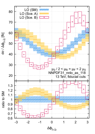
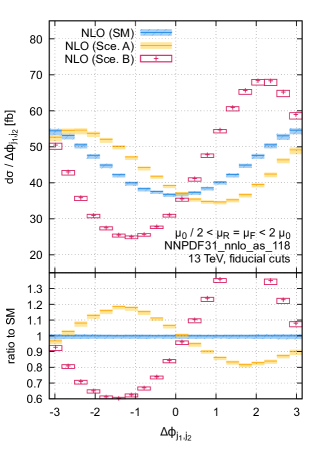
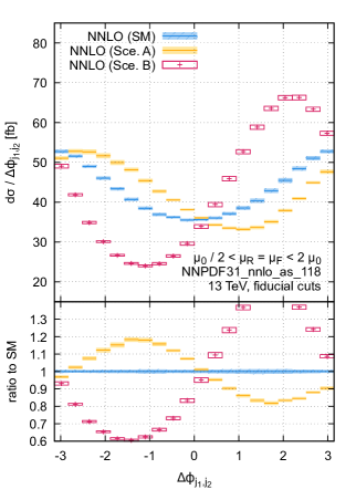
Figure 4: Same as Fig. 3 but for the azimuthal angle difference between the forward and backward VBF tag jets. See text for details.

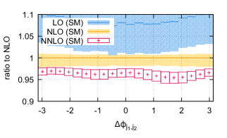
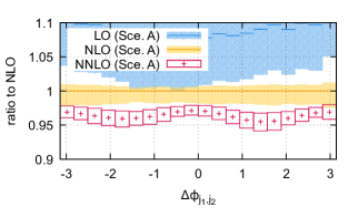
Figure 5: LO (hashed blue) and NNLO (red boxes) predictions for the azimuthal separation between the forward and backward VBF tag jets, divided by the corresponding NLO (solid yellow) result. Left pane: Standard Model. Middle pane: Scenario A. Right pane: Scenario B. The envelope represents scale variation uncertainties. See text for details.

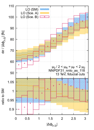
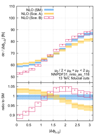
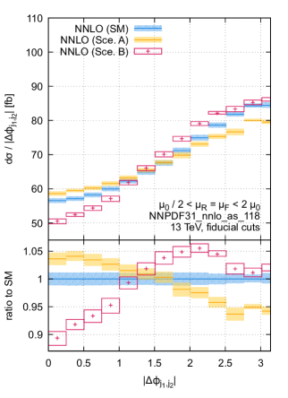
Figure 6: Same as Fig. 4 but for the absolute value of the azimuthal angle difference between the forward and backward VBF tag jets. See text for details.

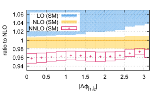
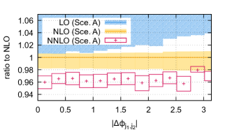
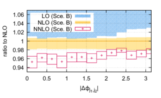
Figure 7: Same as Fig. 5 but for the absolute azimuthal angle separation between the forward and backward VBF tag jets. See text for details.

Differences between scenario A, scenario B and the SM in the distributions shown in Fig. 4 are primarily of an anti-symmetric nature since they are dominated by the interference of $CP$-odd and $CP$-even couplings, which are absent in azimuthally-averaged observables. Hence, in the presence of non-vanishing $CP$-odd EFT operators, this observable may not be optimal to study effects of $CP$-even couplings. To this end, it is useful to consider the absolute value of the azimuthal separation, in which the interference between $CP$-odd and $CP$-even operators drops out Plehn et al. (2002); Figy and Zeppenfeld (2004); Hankele et al. (2006). We show this distribution in Fig. 6.

As expected, the deviations of scenarios A and B from the SM for $|\Delta\phi_{j_{1}j_{2}}|$ in Fig. 6 are much smaller than those observed in Fig. 4. In fact, at LO, the differences between the various scenarios are entirely swamped by scale variation uncertainties. However, despite being less sensitive to non-SM couplings, already at NLO scale uncertainties are sufficiently reduced and the three scenarios become distinguishable. Different shapes of scenarios A and B, due to different $CP$-even contributions, can now be clearly observed. Ratios in Fig. 7 imply that these shapes are also relatively stable under radiative corrections and might, therefore, be captured by global $K$-factors (as was the case for the $\Delta\phi_{j_{1}j_{2}}$ observable).

IV Conclusions

We have studied the combined impact of anomalous Higgs interactions and NNLO QCD corrections on Higgs production in weak boson fusion. For simplicity, we have only considered modifications to the $HVV$ vertex and have performed phenomenological analyses assuming that the modification of the $HWW$ and $HZZ$ couplings are correlated. We have found that the patterns of radiative corrections for the WBF cross section in a typical experimental fiducial region are similar in the Standard Model and when anomalous couplings are present. Namely, in all cases scale variation uncertainties underestimate the size of the correction at the next perturbative order, but predictions seem to be reasonably stable when moving from NLO to NNLO. Keeping in mind that for inclusive SM cross sections the NNLO scale uncertainty band does overlap with N³LO QCD predictions, we have investigated the effect of a reduced theoretical uncertainty on extractions of anomalous couplings. We have studied the constraining power of the fiducial cross section, and found that NLO and NNLO results lead to a similar discriminating power, which is significantly better than the LO one. The relative stability of this picture, when going from NLO to NNLO, gives us confidence that for the analysis of the anomalous couplings in Higgs production through WBF, QCD radiative corrections are sufficiently well understood.

We have also investigated the constraining power of differential distributions, focusing on scenarios where different choices of anomalous couplings led to the same fiducial cross section. It is known that angular distributions have a strong constraining power. However, including NLO QCD corrections is mandatory for differences in shapes induced by small anomalous couplings not to be swamped by theoretical uncertainties. We have shown that theoretical predictions for differential distributions are reasonably stable when moving from NLO to NNLO. In particular, we have found that shape distortions are quite small, and the bulk of the effect of NNLO QCD corrections seems to be captured by a global $K$-factor. We have found that this holds irrespective of the presence or absence of anomalous couplings, at least for the scenarios studied in this paper.

There are several ways in which the analysis presented in this paper can be improved. First, one could study more general scenarios where modifications of the $HZZ$ and $HWW$ couplings are different. Also, one may study the impact of dimension-eight operators in $HVV$ couplings on Higgs signal in WBF. Implementing both of these extensions in our framework is conceptually straightforward. A more involved improvement would be to consider a wider class of higher dimensional operators, especially those that are affected by higher-order QCD corrections. Also, one may consider more realistic setups, where e.g. the decay of the Higgs boson is also taken into account. We look forward to investigating these and other issues relevant for EFT studies in weak boson fusion in the future.

Acknowledgments: We would like to thank Michael Trott for helpful advice regarding the results of Ref. Helset et al. (2020). This research is partially supported by the Deutsche Forschungsgemeinschaft (DFG, German Research Foundation) under grant 396021762 - TRR 257. The research of F.C. was partially supported by the ERC Starting Grant 804394 hipQCD and by the UK Science and Technology Facilities Council (STFC) under grant ST/T000864/1. The research of K.A. is supported by the United States Department of Energy under Grant Contract DE-SC0012704.

References

- Aad et al. (2020) G. Aad et al. (ATLAS), Phys. Rev. D 101, 012002 (2020).
- Sirunyan et al. (2021) A. M. Sirunyan et al. (CMS), Phys. Rev. D 104, 052004 (2021).
- Buchmuller and Wyler (1986) W. Buchmuller and D. Wyler, Nucl. Phys. B 268, 621 (1986).
- Grzadkowski et al. (2010) B. Grzadkowski, M. Iskrzynski, M. Misiak, and J. Rosiek, JHEP 10, 085 (2010).
- Brivio and Trott (2019) I. Brivio and M. Trott, Phys. Rept. 793, 1 (2019).
- Plehn et al. (2002) T. Plehn, D. L. Rainwater, and D. Zeppenfeld, Phys. Rev. Lett. 88, 051801 (2002).
- Figy and Zeppenfeld (2004) T. Figy and D. Zeppenfeld, Phys. Lett. B 591, 297 (2004).
- Hankele et al. (2006) V. Hankele, G. Klamke, D. Zeppenfeld, and T. Figy, Phys. Rev. D 74, 095001 (2006).
- Dreyer and Karlberg (2016) F. A. Dreyer and A. Karlberg, Phys. Rev. Lett. 117, 072001 (2016).
- Cacciari et al. (2015) M. Cacciari, F. A. Dreyer, A. Karlberg, G. P. Salam, and G. Zanderighi, Phys. Rev. Lett. 115, 082002 (2015), [Erratum: Phys.Rev.Lett. 120, 139901 (2018)].
- Cruz-Martinez et al. (2018) J. Cruz-Martinez, T. Gehrmann, E. W. N. Glover, and A. Huss, Phys. Lett. B 781, 672 (2018).
- Asteriadis et al. (2022) K. Asteriadis, F. Caola, K. Melnikov, and R. Röntsch, JHEP 02, 046 (2022).
- Ciccolini et al. (2007) M. Ciccolini, A. Denner, and S. Dittmaier, Phys. Rev. Lett. 99, 161803 (2007).
- Ciccolini et al. (2008) M. Ciccolini, A. Denner, and S. Dittmaier, Phys. Rev. D 77, 013002 (2008).
- Figy et al. (2012) T. Figy, S. Palmer, and G. Weiglein, JHEP 02, 105 (2012).
- Bolzoni et al. (2010) P. Bolzoni, F. Maltoni, S.-O. Moch, and M. Zaro, Phys. Rev. Lett. 105, 011801 (2010).
- Bolzoni et al. (2012) P. Bolzoni, F. Maltoni, S.-O. Moch, and M. Zaro, Phys. Rev. D 85, 035002 (2012).
- Liu et al. (2019) T. Liu, K. Melnikov, and A. A. Penin, Phys. Rev. Lett. 123, 122002 (2019).
- Dreyer et al. (2020) F. A. Dreyer, A. Karlberg, and L. Tancredi, JHEP 10, 131 (2020).
- Denner et al. (2015) A. Denner, S. Dittmaier, S. Kallweit, and A. Mück, Comput. Phys. Commun. 195, 161 (2015).
- Baglio et al. (2014) J. Baglio et al., (2014), arXiv:1404.3940 [hep-ph] .
- Alwall et al. (2011) J. Alwall, M. Herquet, F. Maltoni, O. Mattelaer, and T. Stelzer, JHEP 06, 128 (2011).
- Caola et al. (2017) F. Caola, K. Melnikov, and R. Röntsch, Eur. Phys. J. C 77, 248 (2017).
- Asteriadis et al. (2020) K. Asteriadis, F. Caola, K. Melnikov, and R. Röntsch, Eur. Phys. J. C 80, 8 (2020).
- Helset et al. (2020) A. Helset, A. Martin, and M. Trott, JHEP 03, 163 (2020).
- Mimasu et al. (2016) K. Mimasu, V. Sanz, and C. Williams, JHEP 08, 039 (2016).
- Ball et al. (2017) R. D. Ball et al. (NNPDF), Eur. Phys. J. C 77, 663 (2017).
- Buckley et al. (2015) A. Buckley, J. Ferrando, S. Lloyd, K. Nordström, B. Page, M. Rüfenacht, M. Schönherr, and G. Watt, Eur. Phys. J. C 75, 132 (2015).
- Cacciari et al. (2008) M. Cacciari, G. P. Salam, and G. Soyez, JHEP 04, 063 (2008).