The fewest-big-jumps principle and an

application to random graphs

Céline Kerriou and Peter Mörters

Universität zu Köln

Summary. We prove a large deviation principle for the sum of $n$ independent heavy-tailed random variables, which are subject to a moving truncation at location $n$. Conditional on the sum being large at scale $n$, we show that a finite number of summands take values near the truncation boundary, while the remaining variables still obey the law of large numbers. This generalises the well-known single-big-jump principle for random variables without truncation to a situation where just the minimal necessary number of jumps occur. As an application, we consider a random graph with vertex set given by the lattice points of a torus with sidelength $2N+1$. Every vertex is the centre of a ball with random radius sampled from a heavy-tailed distribution. Oriented edges are drawn from the central vertex to all other vertices in this ball. When this graph is conditioned on having an exceptionally large number of edges we use our main result to show that, as $N\to\infty$, the excess outdegrees condense in a fixed, finite number of randomly scattered vertices of macroscopic outdegree. By contrast, no condensation occurs for the indegrees of the vertices, which all remain microscopic in size.

1 Introduction.

There are two principal paradigms for the upper large deviations of the sum of independent (or mildly dependent) and identically distributed random variables. These are on the one hand the paradigm of collaboration whereby all variables contribute equally to the sum by a change of measure applied to all independent terms. This large deviation strategy typically prevails if the terms are light tailed at infinity and the cost of individual large terms would be overwhelming. On the other hand there is the paradigm of the single big jump, see for example [6, 8, 14], by which a single summand provides a sufficiently large value so that it suffices that all other terms show typical behaviour. In statistical mechanics this paradigm is related to spontaneous symmetry breaking, i.e. a single term is chosen at random to provide the large jump, and condensation, i.e. a single site provides a macroscopic share of the total mass. This large deviation strategy typically prevails in the case of sums of heavy-tailed random variables.

In this paper we look at a situation where the random variables are heavy-tailed but there is a truncation at a variable threshold. In this case a single big jump may not suffice, but rather a finite number of summands are required to provide the large deviation. We prove a precise large deviation result showing that the optimal strategy in this case is to pick the minimal number of sites necessary for the large deviation and share the excess mass among these sites. This result, Theorem 1, underpins the novel paradigm of the minimal number of jumps, or fewest-big-jumps principle, which is at the heart of this paper.

Our general result is motivated by a large deviation principle for the number of edges in a finite geometric random graph model as the number of vertices goes to infinity, see Theorem 4. This model has oriented edges, so that there are two ways to represent the number of edges in the graph as the sum of identically distributed random variables: either as the sum of the indegrees or as the sum of the outdegrees over all vertices in the graph. We show that from the former point of view we see the paradigm of collaboration, but from the latter we see the paradigm of the minimal number of jumps. Our proof of this insightful result uses Theorem 1 applied to the outdegrees. We conclude the paper with some comments on further large deviation results for the number of edges in geometric random graphs.

2 The ‘fewest-big-jumps’ principle.

For our main result we consider a triangular scheme of nonnegative random variables where the random variables $(W_{k}^{{}_{(n)}}\colon k\in[n])$ in the $n$th row are independent and identically distributed to some $W^{{(n)}}$ for which we make the following assumptions.

We have $0\;\leqslant\;W^{{(n)}}\;\leqslant\;n$ and there exists $\alpha>1$ such that the following holds.

1. $(W^{{(n)}})_{n}$ is $L^{p}$-bounded for any $1\;\leqslant\;p<\alpha$.

2. There exists $\mu\;\geqslant\;0$ such that $\mu_{n}:=\mathbb{E}W^{{(n)}}\to\mu$.

3. There exists a regularly varying sequence $(f(n))_{n}$ with index $-\alpha$, a measure $\nu$ on $(0,1]$, which is finite on intervals bounded from zero and absolutely continuous on $(0,1)$ with a continuous density $h\colon(0,1)\to[0,\infty)$, and a sequence $\eta_{n}\downarrow 0$ such that, for all $\varepsilon>0$ whenever $\varepsilon\;\leqslant\;a_{n}<b_{n}$ with $b_{n}\;\leqslant\;1-\eta_{n}$ or $b_{n}=1$ and with $\eta_{n}\;\leqslant\;b_{n}-a_{n}\to 0$, we have

   $$\mathbb{P}(a_{n}n<W^{{(n)}}\;\leqslant\;b_{n}n)=(1+o^{*}(1))\,f(n)\,\nu(a_{n},b_{n}],$$

   where $o^{*}(1)$ is a function going to zero such that, for all fixed $\varepsilon>0$ and $\Delta_{n}\downarrow 0$, the convergence is uniform over all eligible choices of $a_{n},b_{n}$ with $b_{n}-a_{n}\;\leqslant\;\Delta_{n}$.

The measure $\nu$ in Assumption 3 implicitly describes the shape of the truncation on the scale $n$. Observe that $\nu(\{x\})>0$ is allowed only if $x=1$.

Examples: Our examples are based on a random variable $W\;\geqslant\;0$ with regularly varying tail function $G(x):=\mathbb{P}(W>x)$. More precisely, we assume that $G(x)=x^{-\alpha}\ell(x)$ with $\alpha>1$ and the slowly varying part $\ell$ satisfies, for all $0<\varepsilon\;\leqslant\;a_{n}<b_{n}$ with $b_{n}-a_{n}\to 0$,

$$\frac{\ell(b_{n}n)-\ell(a_{n}n)}{\ell(n)\,\frac{b_{n}-a_{n}}{b_{n}}}\to 0\text{ as }n\to\infty,$$ (1)

where for all fixed $\varepsilon>0$ and $\Delta_{n}\downarrow 0$, the convergence is uniform over all choices of $\varepsilon\leq a_{n}<b_{n}$ with $b_{n}-a_{n}\;\leqslant\;\Delta_{n}$. This condition holds, e.g., if $\ell$ is a constant, logarithm, or the reciprocal or iterate of a logarithm.

1. The random variables $W^{{(n)}}:=W\wedge n$ obviously satisfy Assumptions 1 and  2. Moreover, we have for all $n$ with $b_{n}<1$ that

   $$\mathbb{P}(a_{n}n <W\wedge n\;\leqslant\;b_{n}n)={\mathbb{P}}\left(W>a_{n}n\right)-{\mathbb{P}}\left(W>b_{n}n\right)=G(a_{n}n)-G(b_{n}n)$$

   $$=n^{-\alpha}\big{(}(a_{n}^{-\alpha}-b_{n}^{-\alpha})\ell(a_{n}n)+(b_{n}^{-\alpha}(\ell(a_{n}n)-\ell(b_{n}n))\big{)}$$

   $$=n^{-\alpha}\big{(}(a_{n}^{-\alpha}-b_{n}^{-\alpha})(1+o^{*}(1))\ell(n)+o^{*}(1)\ell(n)b_{n}^{-\alpha-1}(b_{n}-a_{n})\big{)}$$

   $$=(1+o^{*}(1))n^{-\alpha}\ell(n)\,(a_{n}^{-\alpha}-b_{n}^{-\alpha}).$$

   and for all $n$ with $b_{n}=1$ that

   $$\mathbb{P}(a_{n}n <W\wedge n\;\leqslant\;b_{n}n)={\mathbb{P}}\left(W>a_{n}n\right)=G(a_{n}n)=n^{-\alpha}a_{n}^{-\alpha}\ell(a_{n}n)$$

   $$=(1+o^{*}(1))n^{-\alpha}\ell(n).$$

   Hence Assumption 3 holds with $f=G$, arbitrary $\eta_{n}\downarrow 0$, and the measure $\nu$ having density $\alpha x^{-\alpha-1}$ on $(0,1)$ and an atom of size one at one.

2. Let $\phi_{n}\colon(0,\infty)\to(0,n)$ be a family of increasing, surjective functions. Suppose $(\phi_{n}(W))_{n}$ is $L^{p}$-bounded for $1\;\leqslant\;p<\alpha$, ${\mathbb{E}}\left[\phi_{n}(W)\right]$ converges and, for some continuously differentiable, increasing function $g\colon(0,1)\to(0,\infty)$ with $g(a)\to\infty$ as $a\uparrow 1$, and for some $\eta_{n}\downarrow 0$ and all $0<\varepsilon\;\leqslant\;a_{n}<b_{n}\;\leqslant\;1$ with $b_{n}-a_{n}\;\geqslant\;{\eta_{n}}$ we have

   $$\sup_{a\in(0,1)}\Big{|}\frac{\phi^{-1}_{n}(an)}{n}-g(a)\Big{|}\;\leqslant\;\eta_{n}^{2}\text{ and }\frac{\ell(\phi^{-1}_{n}(a_{n}n))}{\ell(n)}=1+o^{*}(1).$$ (2)

   Note that by [1, Theorem 1.2.1] the second condition in (2) need only be checked for $a_{n}\to 1$ and ${1-a_{n}}\;\geqslant\;{\eta_{n}}$. We have for $b_{n}<1$ that

   $$\mathbb{P}(a_{n}n <\phi_{n}(W)\;\leqslant\;b_{n}n)={\mathbb{P}}\left(W>\phi_{n}^{-1}(a_{n}n)\right)-{\mathbb{P}}\left(W>\phi_{n}^{-1}(b_{n}n)\right)$$

   $$=\ell(\phi_{n}^{-1}(a_{n}n))\big{(}(\phi_{n}^{-1}(a_{n}n))^{-\alpha}-(\phi_{n}^{-1}(b_{n}n))^{-\alpha}\big{)}$$

   $$\qquad+(\phi_{n}^{-1}(b_{n}n))^{-\alpha}\big{(}\ell(\phi_{n}^{-1}(a_{n}n))-\ell(\phi_{n}^{-1}(b_{n}n))\big{)}$$

   $$=(1+o^{*}(1)){\ell(\phi_{n}^{-1}(a_{n}n))}\big{(}(ng(a_{n}))^{-\alpha}-(ng(b_{n}))^{-\alpha}\big{)}$$

   $$\qquad+o^{*}(1)n^{-\alpha}g(b_{n})^{-\alpha-1}\big{(}\ell(n){(g(a_{n})-g(b_{n}))}\big{)}$$

   $$=(1+o^{*}(1))\ell(n)n^{-\alpha}\,(g(a_{n})^{-\alpha}-g(b_{n})^{-\alpha}),$$

   and, in the case $b_{n}=1$,

   $$\mathbb{P}(a_{n}n<\phi_{n}(W)) ={\mathbb{P}}\left(W>\phi_{n}^{-1}(a_{n}n)\right)=(\phi_{n}^{-1}(a_{n}n))^{-\alpha}{\ell(\phi_{n}^{-1}(a_{n}n))}$$

   $$=(1+o^{*}(1))n^{-\alpha}\ell(n)\,g(a_{n})^{-\alpha}.$$

   Hence $W^{{(n)}}:=\phi_{n}(W)$ satisfies our assumptions with $f=G$ and $\nu$ absolutely continuous with density $h(x)=\alpha g(x)^{-\alpha-1}g^{\prime}(x)$.

   A possible choice of such a truncation family would be $\phi_{n}(x)=n(1-e^{-x/n})$, in which case $\phi_{n}^{-1}(x)=-n\log(1-x/n)$ and $g(x)=-\log(1-x)$. Then the measure $\nu$ is absolutely continuous with density $h(x)=\alpha(1-x)^{-1}\log(\frac{1}{1-x})^{-\alpha-1}$. Given $\ell$ the second condition in (2) becomes a condition on the sequence $(\eta_{n})$.

3. The random variables $W^{{(n)}}$ defined as $W$ conditioned on the event $\{W\;\leqslant\;n\}$ satisfy Assumptions 1 and 2. Moreover, for all $0<\varepsilon\;\leqslant\;a_{n}<b_{n}\;\leqslant\;1$, we have

   $$\mathbb{P}(a_{n}n<W^{{(n)}}\;\leqslant\;b_{n}n)=\frac{G(a_{n}n)-G(b_{n}n)}{1-G(n)}=(1+o^{*}(1))G(n)(a_{n}^{-\alpha}-b_{n}^{-\alpha}),$$

   so that Assumption 3 holds with $f=G$, arbitrary $\eta_{n}\downarrow 0$, and $\nu$ absolutely continuous with density $h(x)=\alpha x^{-\alpha-1}$.

4. Let $W^{{(n)}}$ be the number of points in $B(0,W^{\frac{1}{d}})\cap[-N,N]^{d}\cap\mathbb{Z}^{d}$ where $n=(2N+1)^{d}$. Then we show in Section 3 that $W^{{(n)}}$ satisfies our assumptions.

Theorem 1.

Suppose $W_{1}^{{}_{(n)}},\ldots,W_{n}^{{}_{(n)}}$ are independent random variables satisfying Assumptions 1,  2 and  3, and let

$$S_{n}=W_{1}^{{}_{(n)}}+\ldots+W_{n}^{{}_{(n)}}.$$

Let $\rho>0$ be non-integer and pick the unique $k=k(\rho)\in\mathbb{N}$ such that

$$k-1<\rho<k.$$

Then there exists $\delta_{n}\downarrow 0$ such that, for any two sequences $\rho_{1}(n)\uparrow\rho$ and $\rho_{2}(n)\downarrow\rho$ with $\rho_{2}(n)-\rho_{1}(n)\gg\delta_{n}$, we have

$$\mathbb{P}\big{(}n(\rho_{1}(n)+\mu)\;\leqslant\;S_{n}\;\leqslant\;n(\rho_{2}(n)+\mu)\big{)}=(K_{\rho}+o(1)){n\choose k}(\rho_{2}(n)-\rho_{1}(n))f(n)^{k},$$

where $K_{\rho}:=h(\rho)$ if $0<\rho<1$ and for $\rho>1$,

$$K_{\rho}:=\int\nu(dx_{1})\cdots\int\nu(dx_{k-1})\,\frac{k}{k-\sum_{i=1}^{k-1}1_{x_{i}=1}}\,\,h\Big{(}\rho-\sum_{i=1}^{k-1}x_{i}\Big{)},$$

where $h$ is extended by zero to the entire real line and $K_{\rho}$ is assumed to be finite.

The proof of Theorem 1, given in Section 4, also reveals explicitly how the summands achieve the large deviation of the sum $S_{n}$, namely by making exactly the minimal number $k$ of jumps necessary to increase the sum by $\rho n$. The following corollary makes this observation precise. For the rest of the paper, define for $\rho_{1}(n),\rho_{2}(n)$ as in Theorem 1,

$$I_{n}:=I_{n}(\rho_{1}(n),\rho_{2}(n)):=[n(\rho_{1}(n)+\mu),n(\rho_{2}(n)+\mu)].$$

Corollary 2.

There exists $\gamma_{n}\downarrow 0$ such that for sufficiently small $\varepsilon>0$ we have that

$$\mathbb{P}\Big{(} \text{ there exist exactly }k\text{ indices }i_{1},\ldots,i_{k}\in[n]\text{ such that}$$

$$\phantom{lu}W_{i_{1}}^{{}_{(n)}}>\varepsilon n,\ldots,W_{i_{k}}^{{}_{(n)}}>\varepsilon n\text{ and }\Big{|}\sum_{j=1}^{k}W_{i_{j}}^{{}_{(n)}}-\rho n\Big{|}\;\leqslant\;\gamma_{n}n\text{ and }$$

$$\phantom{lu}W_{j}^{{}_{(n)}}\;\leqslant\;\varepsilon n\,\forall\,j\not=i_{1},\ldots,i_{k}\text{ and }\Big{|}\sum_{\genfrac{}{}{0.0pt}{}{j=1}{j\not=i_{1},\ldots,i_{k}}}^{n}W_{j}^{{}_{(n)}}-\mu n\Big{|}\;\leqslant\;\gamma_{n}n\,\Big{|}\,S_{n}\in I_{n}\Big{)}\rightarrow 1,$$

as $n\rightarrow\infty$.

Before moving to an application of Theorem 1 to random geometric graphs, we state a law of large numbers for the triangular scheme $(W^{(n)}_{k}\colon k\in[n])$ which allows some insight into the possible size of $(\delta_{n})_{n}$ in Theorem 1.

Lemma 3.

There exists $\zeta_{n}\downarrow 0$ such that $S_{n}:=W_{1}^{{}_{(n)}}+\cdots+W_{n}^{{}_{(n)}}$ satisfies

$$\mathbb{P}\big{(}|S_{n}-n\mu|>\zeta_{n}n\big{)}\;\leqslant\;\zeta_{n}.$$

The sequence $(\delta_{n})_{n}$ in Theorem 1 can be chosen as $\delta_{n}\gg\zeta_{n}\vee\eta_{n}$ with $(\eta_{n})_{n}$ as in Assumption 3 and $(\zeta_{n})_{n}$ as in Lemma 3. We additionally require $\zeta_{n}\gg n^{-1}$ and $\zeta_{n}\gg nf(n)$ for $n$ large, which is typically weaker than the requirement of Lemma 3. Explicit values for $(\zeta_{n})_{n}$ can be derived from central or stable limit theorems for the triangular scheme. The proof of Lemma 3 closely follows Feller’s proof of the law of large numbers in [7] and is given for completeness in Section 4.

3 The random graph model.

We now look at a large deviation problem for the number of edges in a geometric random graph model $G=(V,E)$. The vertices of this graph are the $n=(2N+1)^{d}$ lattice points on $\mathbb{T}_{N}:=[-N,N]^{d}$ equipped with the torus metric $D$. Every vertex $v\in V$ is equipped with a random radius $R_{v}\;\geqslant\;0$ where $(R_{v}\colon v\in V)$ are i.i.d. random variables with regularly varying tail function $G(x):=\mathbb{P}(R_{v}>x)$. We assume that $G(x)=x^{-\beta}\ell(x)$ with $\beta>d$ and the slowly varying part $\ell$ satisfies the following condition. For all $0<\varepsilon\;\leqslant\;a_{n}<b_{n}$ with $b_{n}-a_{n}\rightarrow 0$,

$$\frac{\ell(b_{n}n)-\ell(a_{n}n)}{\ell(n)\,\frac{b_{n}-a_{n}}{b_{n}}}\to 0\text{ as }n\to\infty,$$ (3)

where for all fixed $\varepsilon>0$ and $\Delta_{n}\downarrow 0$, the convergence is uniform over all choices of $\varepsilon\leq a_{n}<b_{n}$ with $b_{n}-a_{n}\;\leqslant\;\Delta_{n}$. We draw an oriented edge from each vertex $v$ to all vertices $w\in B(v,R_{v})\setminus\{v\}$, where $B(v,r):=\{w\in\mathbb{T}_{N}\colon D(v,w)<r\}$ is the open ball centred in $v$ of radius $r$.

We denote by $\mathsf{out}(v)$ the out-, and by $\mathsf{in}(v)$ the in-degree of a vertex $v$. Define by

$$\varrho(n):=\frac{1}{n}\sum_{v\in\mathbb{T}_{N}}\mathsf{out}(v)=\frac{1}{n}\sum_{v\in\mathbb{T}_{N}}\mathsf{in}(v)$$

the edge density and by $\displaystyle\mu:=\lim_{n\to\infty}\mathbb{E}\varrho(n)$ the asymptotic mean edge density.

The following theorem is our main application of Theorem 1. It shows that when the graph $G$ is conditioned to have an edge density larger than $\mu$, the excess outdegrees condense in a fixed, finite number of randomly scattered vertices whereas the indegrees all remain microscopic in size.

Theorem 4.

Let $\rho>0$ be non-integer and $k\in{\mathbb{N}}$ such that $k-1<\rho<k$. There exists $\delta_{n}\downarrow 0$ and a constant $K_{\rho}>0$ such that, for any sequences $\rho_{1}(n)\uparrow\rho$ and $\rho_{2}(n)\downarrow\rho$ with $\rho_{2}(n)-\rho_{1}(n)\gg\delta_{n}$, we have

$$\mathbb{P}\big{(}\mu+\rho_{1}(n)\;\leqslant\;\varrho(n)\;\leqslant\;\mu+\rho_{2}(n)\big{)}=(K_{\rho}+o(1)){n\choose k}(\rho_{2}(n)-\rho_{1}(n))\,G(n)^{k/d}.$$

Given the event $\{\mu+\rho_{1}(n)\;\leqslant\;\varrho(n)\;\leqslant\;\mu+\rho_{2}(n)\}$ we have that

1. there exists a set $\mathscr{V}$ of exactly $k$ vertices $v_{1},\ldots,v_{k}\in\mathbb{T}_{N}$ such that

   $$\lim_{n\to\infty}\frac{1}{n}\sum_{i=1}^{k}\mathsf{out}(v_{i})=\rho\qquad\mbox{ in probability. }$$

2. every $v\in\mathscr{V}$ has a macroscopic share of the total outdegree, i.e. there exists $\varepsilon>0$ such that

   $$\min_{v\in\mathscr{V}}\frac{\mathsf{out}(v)}{n}\;\geqslant\;\varepsilon\qquad\mbox{ with high probability,}$$

   whereas every $v\not\in\mathscr{V}$ makes only a microscopic contribution, i.e.

   $$\lim_{n\to\infty}\max_{v\not\in\mathscr{V}}\frac{\mathsf{out}(v)}{n}=0\qquad\mbox{ in probability.}$$

3. no vertex makes a macroscopic contribution to the total indegree, i.e.

   $$\lim_{n\to\infty}\max_{v\in V}\frac{\mathsf{in}(v)}{n}=0\qquad\mbox{ in probability.}$$

Proof.

For every vertex $v\in V$, define $W^{{}_{(n)}}_{v}$ to be the outdegree of $v$, that is, $W^{{}_{(n)}}_{v}$ is the number of lattice points in $(B(v,R_{v})\setminus\{v\})\cap\mathbb{T}_{N}$. Then $(W^{{}_{(n)}}_{v}:v\in V)$ are independent, identically distributed and $\varrho(n)=\sum_{v\in V}W^{{}_{(n)}}_{v}/n$. We claim that $W^{(n)}_{v}$ satisfies Assumptions 1,  2 and  3 with $\alpha=\beta/d$ and $f(n)=G(n)^{1/d}$. The first equality of Theorem 4 then follows directly by Theorem 1, and (a) and (b) follow from Corollary 2. To see why (c) holds, assume that the indegree of some vertex $v\in V$ is of order $n$. Then $v$ is contained in at least order $n^{(d-1)/d}$ balls of volume of order $n$. In other words, there are at least order $n^{(d-1)/d}$ vertices with outdegree of order $n$, which contradicts (b).

The random variables $W^{(n)}=W^{{}_{(n)}}_{0}$ satisfy Assumption 1 as they are bounded by a constant multiple of $R_{0}^{d}$. As $\beta>d$, the Potter bounds (see [1, Theorem 1.5.6]) give us that for $1\;\leqslant\;p<\alpha=\beta/d$ and some constant $c>0$, $\mathbb{E}[|W^{(n)}|^{p}]\;\leqslant\;c^{p}\mathbb{E}[R_{0}^{dp}]<\infty$. Assumption 2 follows from the fact that $\smash{(W^{(n)})_{n}}$ is increasing to the number of lattice points in $B(0,R_{0})\setminus\{0\}$. We are left to show that $W^{(n)}$ satisfies Assumption 3 with $\alpha=\beta/d$ and $f(n)=G(n)^{1/d}$. We do so by bounding $W^{(n)}$ from below, resp. above, by the number of unit hypercubes (centred in lattice points) that are contained in, resp. intersect, $(B(0,R_{0})\setminus\{0\})\cap\mathbb{T}_{N}$. Define the function $g:[0,\infty)\rightarrow[0,1]$ by

$$g(r):=\text{Vol}(B(0,\tfrac{1}{2}\sqrt{d}r)\cap\left[-1/2,1/2\right]^{d}).$$

Then $g(r)=1$ for $r\;\geqslant\;1$. Note that $g^{\prime}(r)$ corresponds to the $(d-1)$-dimensional Hausdorff measure of the sphere $\partial B(0,\frac{1}{2}\sqrt{d}r)$ intersected with the set $[-1/2,1/2]^{d}$. Therefore $g$ is strictly increasing and continuously differentiable on $(0,1)$ and we have $g^{\prime}(x)>0$ for all $x\in(0,1)$. Moreover,

$$\lim_{x\downarrow 0}g^{\prime}(x)=0\text{ and }\lim_{x\uparrow 1}g^{\prime}(x)=0.$$

Hence $g^{-1}\colon(0,1)\rightarrow(0,1)$ is continuously differentiable and strictly increasing. Observe that with $g^{-1}(1)=1$, for all $0<a\;\leqslant\;1$ and $0<\varepsilon<a$, we get that

$$\big{|}g^{-1}(a)-g^{-1}(a-\varepsilon)\big{|}\;\leqslant\;\varepsilon^{1/d}.$$ (4)

To see this first for $a=1$ note that $g(1)-g(1-\varepsilon)$ is the volume of the intersection $S_{\varepsilon}$ of $[-1/2,1/2]^{d}$ and the complement of the ball $B(0,(1-\varepsilon)\sqrt{d}/2)$. Let $y=\varepsilon\sqrt{d}/2$ be the distance between a corner of $[-1/2,1/2]^{d}$ and the ball. At each corner we can fit an open cube with diagonal $y$ into $S_{\varepsilon}$, as illustrated in Figure 2. As $[-1/2,1/2]^{d}$ has $2^{d}$ corners we can bound $g(1)-g(1-\varepsilon)$ from below by $2^{d}(y/\sqrt{d})^{d}=\varepsilon^{d}$. Since $g^{-1}(1)=1$ and $g^{-1}$ is strictly increasing, we have that $1-\varepsilon\;\leqslant\;g^{-1}(1-\varepsilon^{d})$ and we can can conclude that (4) holds for $a=1$. For $0<x<1$ an analogous argument gives $x-\varepsilon\leq g^{-1}(g(x)-\varepsilon^{d})$ and plugging $x=g^{-1}(a)$ implies the result for any $0<a<1$.

We can express the volume of the intersection of a ball of radius $r>0$ and $\mathbb{T}_{N}$ in terms of $g$ as

$$\text{Vol}(B(0,r)\cap\mathbb{T}_{N}) =(2N)^{d}g\big{(}\tfrac{r}{\sqrt{d}N}\big{)}.$$

Note that the boundary of $B(0,r)$ intersects a constant multiple of $N^{d-1}$ unit hypercubes centred in lattice points of $\mathbb{T}_{N}$. We bound $W^{(n)}$ from above by the smallest number of unit hypercubes needed to cover $B(0,R_{0})\cap\mathbb{T}_{N}$. This in turn can be bounded by the volume of $B(0,R_{0})\cap\mathbb{T}_{N}$ summed with the number of unit hypercubes in $\mathbb{T}_{N}$ intersecting its boundary. A lower bound follows analogously. An illustration appears in Figure 2. Thus it holds that for some constant $c_{d}>1$,

$$(2N)^{d}g\big{(}\tfrac{R_{0}}{\sqrt{d}N}\big{)}-c_{d}N^{d-1}\;\leqslant\;W^{(n)}\;\leqslant\;(2N)^{d}g\big{(}\tfrac{R_{0}}{\sqrt{d}N}\big{)}+c_{d}N^{d-1}.$$

Figure 1: The figure illustrates how an open cube of sidelength $y/\sqrt{d}$ can be fit into $S_{\varepsilon}$.

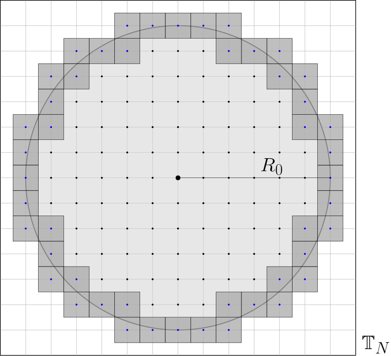
Figure 2: The figure illustrates how $W^{(n)}$ can be bounded from above by the volume of $B(0,R_{0})$ plus the number of unit cubes in $\mathbb{T}_{N}$ that intersect the boundary of the ball. A lower bound follows by subtracting the number of unit cubes in $\mathbb{T}_{N}$ intersecting the boundary of the ball from its volume.

Recalling that $n=(2N+1)^{d}$, it follows that for all $\varepsilon>0$ and $\varepsilon\;\leqslant\;a_{n}<b_{n}\;\leqslant\;1$ there exists some constant $c_{d}^{\prime}>0$ such that for sufficiently large $n$,

$${\mathbb{P}}\left(W^{(n)}>a_{n}n\right) \;\leqslant\;{\mathbb{P}}\left(g(\tfrac{R_{0}}{\sqrt{d}N})>a_{n}-c^{\prime}_{d}N^{-1}\right)={\mathbb{P}}\left(R_{0}>\sqrt{d}Ng^{-1}(a_{n}-c_{d}^{\prime}N^{-1})\right)$$

$$=G\big{(}\sqrt{d}Ng^{-1}(a_{n}-c_{d}^{\prime}N^{-1})\big{)},$$

and similarly, for $1-b_{n}\gg N^{-1}$, we have

$${\mathbb{P}}\left(W^{(n)}>b_{n}n\right) \;\geqslant\;G\big{(}\sqrt{d}Ng^{-1}(b_{n}+c_{d}^{\prime}N^{-1})\big{)}.$$

By our assumption on $G$ we have, for all $\varepsilon>0$ and $\varepsilon\;\leqslant\;c_{n}<d_{n}\;\leqslant\;1$ with $d_{n}-c_{n}\to 0$,

$$G(c_{n}N)-G(d_{n}N) =N^{-\beta}((c_{n}^{-\beta}-d_{n}^{-\beta})\ell(c_{n}N)+d_{n}^{-\beta}(\ell(c_{n}N)-\ell(d_{n}N)))$$

$$=N^{-\beta}((c_{n}^{-\beta}-d_{n}^{-\beta})(1+o^{*}(1))\ell(N)+o^{*}(1)\ell(N)d_{n}^{-\beta-1}(c_{n}-d_{n})$$

$$=(1+o^{*}(1))N^{-\beta}\ell(N)\,(c_{n}^{-\beta}-d_{n}^{-\beta}).$$ (5)

For $1-b_{n}\;\geqslant\;\eta_{n}\gg N^{-1}$, by (4), we can write $g^{-1}(a_{n}-c_{d}^{\prime}N^{-1})=g^{-1}(a_{n})-\delta_{n}$ and $g^{-1}(b_{n}+c_{d}^{\prime}N^{-1})=g^{-1}(b_{n})+\delta^{\prime}_{n}$ for some $0\;\leqslant\;\delta_{n},\delta^{\prime}_{n}\;\leqslant\;(c_{d}^{\prime}N^{-1})^{1/d}$. We infer by (3) that, for some constant $c_{d}^{\prime\prime}>0$ we have that

$${\mathbb{P}}\left(a_{n}n<W^{(n)}\;\leqslant\;b_{n}n\right)\;\leqslant\;G\big{(}\sqrt{d}Ng^{-1}(a_{n}-c_{d}^{\prime}N^{-1})\big{)}-G\big{(}\sqrt{d}Ng^{-1}(b_{n}+c_{d}^{\prime}N^{-1})\big{)}$$

$$\qquad=(1+o^{*}(1))N^{-\beta}\ell(N)\,{d}^{-\beta/2}\,(g^{-1}(a_{n}-c_{d}^{\prime}N^{-1})^{-\beta}-g^{-1}(b_{n}+c_{d}^{\prime}N^{-1})^{-\beta})$$

$$\qquad\;\leqslant\;(1+o^{*}(1))G(N)\,{d}^{-\beta/2}\,\big{(}g^{-1}(a_{n})^{-\beta}-g^{-1}(b_{n})^{-\beta}+c_{d}^{\prime\prime}N^{-1/d}\big{)}.$$

If $b_{n}-a_{n}\;\geqslant\;\eta_{n}\gg N^{-1/d}$, then

$$g^{-1}(a_{n})^{-\beta}-g^{-1}(b_{n})^{-\beta}+c_{d}^{\prime\prime}N^{-1/d}=(1+o^{*}(1))\int_{a_{n}}^{b_{n}}-((g^{-1})^{-\beta})^{\prime}(x)\,dx.$$

A matching lower bound on ${\mathbb{P}}\left(a_{n}n<W^{(n)}\;\leqslant\;b_{n}n\right)$ follows analogously. In the case $b_{n}=1$, we get

$$\mathbb{P}(W^{(n)} >a_{n}n)\;\leqslant\;G\big{(}\sqrt{d}Ng^{-1}(a_{n}-c_{d}^{\prime}N^{-1})\big{)}$$

$$=(1+o^{*}(1))G(N)\big{(}\sqrt{d}g^{-1}(a_{n}-c_{d}^{\prime}N^{-1})\big{)}^{-\beta}=(1+o^{*}(1))G(N)d^{-\beta/2},$$

where the second equality holds as $a_{n}-c^{\prime}dN^{-1}$ tends to one and $g^{-1}(1)=1$. In the same manner, we deduce a matching lower bound. Now, define the function $h:(0,1)\rightarrow(0,\infty)$ by

$$h(x):=-d^{-\beta/2}((g^{-1})^{-\beta})^{\prime}(x),\quad\mbox{ for }x\in(0,1).$$

Note that $h$ is continuous and integrable on intervals bounded from zero. Combining the above, we conclude that $W^{(n)}$ satisfies Assumption 3 with $\eta_{n}\gg N^{-1/d}\sim 2^{1/d}n^{-1/d^{2}}$, $f(n)=G(N)\sim 2^{-\beta}G(n^{1/d})$ and a measure $\nu$ with density $h$ on $(0,1)$ and an atom of size $d^{-\beta/2}$ at one. ∎

4 Proof of Theorem 1.

In Theorem 1 we claim that the large value of $S_{n}$ is achieved by increasing exactly $k$ of the summands $W_{1}^{{}_{(n)}},\ldots,W_{n}^{{}_{(n)}}$ to size of order $n$, so that together they give an extra contribution of $\rho n$. We start the proof by Lemma 5, which is a useful tool that in particular allows us to calculate the probability of this principal strategy. The proof is then completed by four claims. Claim 1 shows that the principal strategy is successful, i.e. it leads to the desired value of $S_{n}$. We classify possible alternative strategies into three categories:

• exactly $k$ summands are of order $n$ but their joint contribution is not $\rho n$,

• more than $k$ summands are of order $n$,

• fewer than $k$ summands are of order $n$.

We show in Claims 2–4 that the probability of each of the three above strategies is of strictly smaller order than that of the principal strategy.

Similar methods of proof have been used to show big jump principles, see for example [11, 10, 2], and [12, 4] for a different approach. Our proof is modelled on the ideas of Janson [10, Theorem 19.34] for balls-in-boxes models and random trees, which has the combined advantage of giving a very precise result and including information about the geometry of the conditional sample as given in our Corollary 2. We generalise Janson’s technique by removing restrictions on the discrete nature of the random variables, dealing with variables that may be continuous or discrete, possibly with a complex lattice structure, and of course by incorporating the truncation effect. For $k>1$ the latter leads to significant additional difficulties in the argument as extra randomness has to be controlled coming from different possible distributions of the mass among the $k$ condensates. The proof collapses and no analogous result holds when $\rho$ is an integer, as in this case the necessary number of condensates is not constant over the target interval $I_{n}$.

We start the proof of Theorem 1 with a local limit theorem for finite sums of independent random variables satisfying Assumptions 1, 2 and 3.

Lemma 5.

Let $k$ be a fixed integer with $k-1<\rho<k$ and

$$T_{k}=T_{k}(n):=W_{1}^{{}_{(n)}}+\cdots+W_{k}^{{}_{(n)}}.$$

For any sequences $\sigma_{1}(n)\uparrow\rho,\sigma_{2}(n)\downarrow\rho$ with $\sigma_{2}(n)-\sigma_{1}(n)\gg\eta_{n}$, we have that

$${\mathbb{P}}\left(n\sigma_{1}(n)\;\leqslant\;T_{k}\;\leqslant\;n\sigma_{2}(n)\right) =(K_{\rho}+o(1))(\sigma_{2}(n)-\sigma_{1}(n))\,{f(n)}^{k}.$$

Proof of Lemma 5.

Let $\sigma_{1}(n)\uparrow\rho,\sigma_{2}(n)\downarrow\rho$ be such that $\sigma_{2}(n)-\sigma_{1}(n)\gg\eta_{n}$. Fix a small $\varepsilon>0$ and let $\Delta_{n}\downarrow 0$ be a sequence satisfying $\eta_{n}\ll\Delta_{n}\ll\sigma_{2}(n)-\sigma_{1}(n)$ and $m=(1-\varepsilon)/\Delta_{n}\in{\mathbb{N}}$. Fix a partition $P_{n}=\{t_{0},\ldots,t_{m}\}$ of $[\varepsilon,1]$ satisfying $|t_{i}-t_{i-1}|=\Delta_{n}$ for all $i\in[m]$. We begin by constructing a lower bound of ${\mathbb{P}}\left(n\sigma_{1}(n)\;\leqslant\;T_{k}\;\leqslant\;n\sigma_{2}(n)\right)$. Note that

$${\mathbb{P}}\left(n\sigma_{1}(n)\;\leqslant\;T_{k}\;\leqslant\;n\sigma_{2}(n)\right)$$

$$\;\geqslant\;\sum_{\begin{subarray}{c}(\ell_{1},\ldots,\ell_{k})\in[m]^{k}\end{subarray}}\prod_{j=1}^{k}{\mathbb{P}}\left(nt_{\ell_{j}-1}<W_{j}^{{}_{(n)}}\;\leqslant\;nt_{\ell_{j}}\right){\mathbf{1}}_{\left[\sigma_{1}(n)\;\leqslant\;\sum_{j\in[k]}t_{\ell_{j}-1},\sum_{j\in[k]}t_{\ell_{j}}\;\leqslant\;\sigma_{2}(n)\right]}$$

$$=(1+o(1))f(n)^{k}\sum_{\begin{subarray}{c}(\ell_{1},\ldots,\ell_{k})\in[m]^{k}\\ \sum_{j\in[k]}t_{\ell_{j}-1}\;\geqslant\;\sigma_{1}(n)\\ \sum_{j\in[k]}t_{\ell_{j}}\;\leqslant\;\sigma_{2}(n)\end{subarray}}\prod_{j=1}^{k}\nu(t_{\ell_{j}-1},t_{\ell_{j}}]$$

$$\;\geqslant\;(1+o(1))f(n)^{k}\nu^{k}\big{\{}(x_{1},\ldots,x_{k})\in(\varepsilon,1]^{k}\colon\sigma_{1}(n)+k\Delta_{n}\;\leqslant\;\sum_{j=1}^{k}x_{j}\;\leqslant\;\sigma_{2}(n)-k\Delta_{n}\big{\}},$$

where the equality holds by Assumption 3. To see why the last inequality holds, note that as $P_{n}$ is a partition of $[\varepsilon,1]$, for any $(x_{1},\ldots,x_{k})\in(\varepsilon,1]^{k}$ we can find $(\ell_{1},\ldots,\ell_{k})\in[m]^{k}$ such that $x_{i}\in(t_{\ell_{i}-1},t_{\ell_{i}}]$ for each $i\in[k]$. Further, we know that $t_{\ell_{i}-1}=t_{\ell_{i}}-\Delta_{n}$. Thus if $x_{1}+\cdots+x_{k}\;\geqslant\;\sigma_{1}(n)+k\Delta_{n}$ then $\sum_{j\in[k]}t_{\ell_{j}-1}=\sum_{j\in[k]}t_{\ell_{j}}-k\Delta_{n}\;\geqslant\;\sum_{j\in[k]}x_{j}-k\Delta_{n}\;\geqslant\;\sigma_{1}(n)$. Similarly if $x_{1}+\cdots+x_{k}\;\leqslant\;\sigma_{2}(n)-k\Delta_{n}$ then $\sum_{j\in[k]}t_{\ell_{j}}\;\leqslant\;\sigma_{2}(n)$.

Given $\bm{x}=(x_{1},\ldots,x_{k})\in(\varepsilon,1]^{k}$ we let $j(\bm{x})$ be the number of entries in $\bm{x}$ that are equal to one and let $c:=\nu(\{1\})$. We rewrite

$$\nu^{k}\big{\{}\bm{x}=(x_{1},\ldots,x_{k})\in(\varepsilon,1]^{k}\colon j(\bm{x})=j,\,\sigma_{1}(n)+k\Delta_{n}\;\leqslant\;\sum_{i=1}^{k}x_{i}\;\leqslant\;\sigma_{2}(n)-k\Delta_{n}\big{\}}$$

$$=c^{j}{k\choose j}\int_{(\varepsilon,1)}\nu(dx_{1})\cdots\int_{(\varepsilon,1)}\nu(dx_{k-j-1})$$

$$\phantom{didudeldidoe}\int_{\sigma_{1}(n)+k\Delta_{n}-(x_{1}+\cdots+x_{k-j-1}+j)}^{\sigma_{2}(n)-k\Delta_{n}-(x_{1}+\cdots+x_{k-j-1}+j)}h{\mathbf{1}}_{(\varepsilon,1)}(x)\,dx.$$

Since $\sigma_{2}(n)-k\Delta_{n}$ and $\sigma_{1}(n)+k\Delta_{n}$ both converge to $\rho>k-1$ as $n$ tends to infinity, we have $\sigma_{2}(n)-\sigma_{1}(n)-2k\Delta_{n}=(1+o(1))(\sigma_{2}(n)-\sigma_{1}(n))$ by choice of $\Delta_{n}$. This is asymptotically equivalent to

$$(\sigma_{2}(n)-\sigma_{1}(n))c^{j}{k\choose j}\int_{(\varepsilon,1)}\nu(dx_{1})\cdots\int_{(\varepsilon,1)}\nu(dx_{k-j-1})\,h{\mathbf{1}}_{(\varepsilon,1)}\Big{(}\rho-j-\sum_{i=1}^{k-j-1}x_{i}\Big{)}.$$

By the monotone convergence theorem, since $h$ is non-negative, the integral converges, as $\varepsilon$ tends to zero, to

$$\int_{(0,1)}\nu(dx_{1})\cdots\int_{(0,1)}\nu(dx_{k-j-1})\,h\Big{(}\rho-j-\sum_{i=1}^{k-j-1}x_{i}\Big{)}.$$

Summing over $j$ from 0 to $k-1$ gives

$$(\sigma_{2}(n)-\sigma_{1}(n))\int\nu(dx_{1})\cdots\int\nu(dx_{k-1})\,\frac{k}{k-\sum_{i=1}^{k-1}{\mathbf{1}}_{\left[x_{i}=1\right]}}\,\,h\Big{(}\rho-\sum_{i=1}^{k-1}x_{i}\Big{)},$$

and the desired lower bound follows.

Next, we construct an upper bound. Let $0<\varepsilon<\rho-(k-1)$ and observe that for $n$ sufficiently large $n\sigma_{1}(n)\;\leqslant\;T_{k}\;\leqslant\;n\sigma_{2}(n)$ implies $W_{i}^{{}_{(n)}}\geq\varepsilon n$ for all $i\in[k]$. It follows that, for large $n$,

$${\mathbb{P}}\left(n\sigma_{1}(n)\;\leqslant\;T_{k}\;\leqslant\;n\sigma_{2}(n)\right)$$

$$={\mathbb{P}}\left(n\sigma_{1}(n)\;\leqslant\;T_{k}\;\leqslant\;n\sigma_{2}(n)\text{ and }W_{i}^{{}_{(n)}}\;\geqslant\;\varepsilon n\,\,\text{for all }i\in[k]\right)$$

$$\;\leqslant\;\sum_{\begin{subarray}{c}(\ell_{1},\ldots,\ell_{k})\in[m]^{k}\end{subarray}}\prod_{j=1}^{k}{\mathbb{P}}\left(nt_{\ell_{j}-1}<W_{j}^{{}_{(n)}}\;\leqslant\;nt_{\ell_{j}}\right){\mathbf{1}}_{\left[\sum_{j\in[k]}t_{\ell_{j}-1}\;\leqslant\;\sigma_{2}(n),\sum_{j\in[k]}t_{\ell_{j}}\;\geqslant\;\sigma_{1}(n)\right]}$$

$$=(1+o(1))f(n)^{k}\sum_{\begin{subarray}{c}(\ell_{1},\ldots,\ell_{k})\in[m]^{k}\\ \sum_{j\in[k]}t_{\ell_{j}-1}\;\leqslant\;\sigma_{2}(n)\\ \sum_{j\in[k]}t_{\ell_{j}}\;\geqslant\;\sigma_{1}(n)\end{subarray}}\prod_{j=1}^{k}\nu(t_{\ell_{j}-1},t_{\ell_{j}}]$$

$$\;\leqslant\;(1+o(1))f(n)^{k}\nu^{k}\big{\{}(x_{1},\ldots,x_{k})\in(\varepsilon,1]^{k}\colon\sigma_{1}(n)-k\Delta_{n}\;\leqslant\;\sum_{j=1}^{k}x_{j}\;\leqslant\;\sigma_{2}(n)+k\Delta_{n}\big{\}},$$

where the last inequality follows from the fact that if $\sum_{j\in[k]}t_{\ell_{j}}\;\geqslant\;\sigma_{1}(n)$, then $\sigma_{1}(n)\;\leqslant\;\sum_{j\in[k]}t_{\ell_{j}}=\sum_{j\in[k]}t_{\ell_{j}-1}+k\Delta_{n}\;\leqslant\;\sum_{j\in[k]}x_{j}+k\Delta_{n}$. Similarly, if we have $\sum_{j\in[k]}t_{\ell_{j}-1}\;\leqslant\;\sigma_{2}(n)$, then $\sum_{j\in[k]}x_{j}\;\leqslant\;\sigma_{2}(n)+k\Delta_{n}$. We can bound the measure from above by replacing $(\varepsilon,1)^{k}$ by $(0,1)^{k}$. Arguing as in the proof of the lower bound we can conclude the desired result.∎

With this tool at hand we now focus on the proof of Theorem 1. Let $\delta_{n}\gg\zeta_{n}\vee\eta_{n}$ with $\zeta_{n}\downarrow 0$ be a sequence given by Lemma 3. As previously remarked, we can assume that $\delta_{n}>n^{1-\alpha}\vee n^{-1}$ for all $n\;\geqslant\;0$. Let $\rho_{1}(n)\uparrow\rho$ and $\rho_{2}(n)\downarrow\rho$ be sequences satisfying $\rho_{2}(n)-\rho_{1}(n)\gg\delta_{n}$. Fix $\varepsilon$ such that

$$0<\varepsilon<(\alpha-1)(\rho-(k-1))/(2+k\alpha)$$ (6)

and recall the definition of the interval

$$I_{n} :=I_{n}(\rho_{1}(n),\rho_{2}(n)):=[n(\rho_{1}(n)+\mu),n(\rho_{2}(n)+\mu)].$$

The choice of $\varepsilon$ will be relevant in the proof of Claim 4. Further, for $m\in[n]$ define $T_{m}=T_{m}(n):=W_{1}^{{}_{(n)}}+\cdots+W_{m}^{{}_{(n)}}$. To accommodate for error terms we introduce two sequences $(\rho^{\subset}_{1}(n))_{n}$ and $(\rho^{\subset}_{2}(n))_{n}$ converging to $\rho$ satisfying $\rho_{1}(n)+\delta_{n}<\rho^{\subset}_{1}(n)<\rho_{1}(n)+2\delta_{n}$ and $\rho_{2}(n)-2\delta_{n}<\rho^{\subset}_{2}(n)<\rho_{2}(n)-\delta_{n}$ for all $n\;\geqslant\;1$. Note that $\rho^{\subset}_{2}(n)-\rho^{\subset}_{1}(n)=(1+o(1))(\rho_{2}(n)-\rho_{1}(n))$. We decompose $\{S_{n}\in I_{n}\}$ into disjoint events and study their individual probabilities. Define the following events.

$$\mathcal{E}_{1}:\, S_{n}\in I_{n},\text{ there exist exactly $k$ indices $i_{1},\ldots,i_{k}\in[n]$ such that}$$

$$W_{i_{1}}^{{}_{(n)}}>\varepsilon n,\ldots,W_{i_{k}}^{{}_{(n)}}>\varepsilon n,\text{ and }W_{i_{1}}^{{}_{(n)}}+\cdots+W_{i_{k}}^{{}_{(n)}}\in[n\rho^{\subset}_{1}(n),n\rho^{\subset}_{2}(n)].$$

$$\mathcal{E}_{2}:\, S_{n}\in I_{n},\text{ there exist exactly $k$ indices $i_{1},\ldots,i_{k}\in[n]$ such that }$$

$$\text{$W_{i_{1}}^{{}_{(n)}}>\varepsilon n$,\ldots, $W_{i_{k}}^{{}_{(n)}}>\varepsilon n$, and }W_{i_{1}}^{{}_{(n)}}+\cdots+W_{i_{k}}^{{}_{(n)}}\not\in[n\rho^{\subset}_{1}(n),n\rho^{\subset}_{2}(n)].$$

$$\mathcal{E}_{3}:\, S_{n}\in I_{n},\text{ $W_{i}^{{}_{(n)}}>\varepsilon n$ for at least $k+1$ indices $i\in[n]$.}$$

$$\mathcal{E}_{4}^{j}:\, S_{n}\in I_{n},\text{ there are exactly $j$ indices $i_{1},\ldots,i_{j}$ such that }$$

$$W_{i_{1}}^{{}_{(n)}}>\varepsilon n,\ldots,W_{i_{j}}^{{}_{(n)}}>\varepsilon n.$$

We can then rewrite $\{S_{n}\in I_{n}\}$ as a union of disjoint events,

$$\{S_{n}\in I_{n}\}=\mathcal{E}_{1}\cup\mathcal{E}_{2}\cup\mathcal{E}_{3}\cup\bigcup_{j=0}^{k-1}\mathcal{E}_{4}^{j}.$$ (7)

The proof consists in showing that $\mathcal{E}_{1}$ is the dominating event and that the probabilities of the events $\mathcal{E}_{2},\mathcal{E}_{3},\mathcal{E}_{4}^{j}$ for $0\;\leqslant\;j\;\leqslant\;k-1$ are of smaller order than ${\mathbb{P}}\left(\mathcal{E}_{1}\right)$. Define the following events for $\{i_{1},\ldots,i_{k+1}\}\subset[n]$,

$$\mathcal{E}_{1;i_{1}\ldots i_{k}}:\, S_{n}\in I_{n},\,W_{i_{1}}^{{}_{(n)}}+\cdots+W_{i_{k}}^{{}_{(n)}}\in[n\rho^{\subset}_{1}(n),n\rho^{\subset}_{2}(n)]\ \text{ and }$$

$$W_{i_{1}}^{{}_{(n)}}>\varepsilon n,\ldots,W_{i_{k}}^{{}_{(n)}}>\varepsilon n,\,W_{j}^{{}_{(n)}}\;\leqslant\;\varepsilon n\,\forall j\notin\{i_{1},\ldots,i_{k}\},$$

$$\mathcal{E}_{2;i_{1}\ldots i_{k}}:\, S_{n}\in I_{n},\,W_{i_{1}}^{{}_{(n)}}+\cdots+W_{i_{k}}^{{}_{(n)}}\notin[n\rho^{\subset}_{1}(n),n\rho^{\subset}_{2}(n)]\text{ and }$$

$$W_{i_{1}}^{{}_{(n)}}>\varepsilon n,\ldots,W_{i_{k}}^{{}_{(n)}}>\varepsilon n,$$

$$\mathcal{E}_{3;i_{1}\ldots i_{k}i_{k+1}}:\, S_{n}\in I_{n},W_{i_{1}}^{{}_{(n)}}>\varepsilon n,\ldots,W_{i_{k+1}}^{{}_{(n)}}>\varepsilon n.$$

The identities below follow immediately.

$${\mathbb{P}}\left(\mathcal{E}_{1}\right) ={n\choose{k}}{\mathbb{P}}\left(\mathcal{E}_{1;12\ldots k}\right),$$ (8)

$${\mathbb{P}}\left(\mathcal{E}_{2}\right) \;\leqslant\;{n\choose{k}}{\mathbb{P}}\left(\mathcal{E}_{2;12\ldots k}\right),$$ (9)

$${\mathbb{P}}\left(\mathcal{E}_{3}\right) \;\leqslant\;{n\choose{k+1}}{\mathbb{P}}\left(\mathcal{E}_{3;12\ldots k\,k+1}\right).$$ (10)

Further, we claim that the following equalities hold.

Claim 1.

${\mathbb{P}}\left(\mathcal{E}_{1;12\ldots k}\right)=(1+o(1)){\mathbb{P}}\left(n\rho^{\subset}_{1}(n)\;\leqslant\;T_{k}\;\leqslant\;n\rho^{\subset}_{2}(n)\right).$

Claim 2.

${\mathbb{P}}\left(\mathcal{E}_{2;12\ldots k}\right)=o((\rho_{2}(n)-\rho_{1}(n))f(n)^{k}).$

Claim 3.

${\mathbb{P}}\left(\mathcal{E}_{3;12\ldots k\,k+1}\right)=o((\rho_{2}(n)-\rho_{1}(n))n^{-1}f(n)^{k}).$

Claim 4.

For $0\;\leqslant\;j<k$, we have ${\mathbb{P}}\left(\mathcal{E}^{j}_{4}\right)=o(n^{-1}n^{k}f(n)^{k}).$

By (8), Claim 1 and Lemma 5 we then have that

$${\mathbb{P}}\left(\mathcal{E}_{1}\right)=(1+o(1)){n\choose{k}}(\rho^{\subset}_{2}(n)-\rho^{\subset}_{1}(n))f(n)^{k}K_{\rho}.$$

Combining the identities and claims above, together with (7), the fact that $\rho^{\subset}_{2}(n)-\rho^{\subset}_{1}(n)=(1+o(1))(\rho_{2}(n)-\rho_{1}(n))$ and $\rho_{2}(n)-\rho_{1}(n)\gg\delta_{n}>n^{-1}$ gives

$${\mathbb{P}}\left(S_{n}\in I_{n}\right)=(1+o(1)){\mathbb{P}}\left(\mathcal{E}_{1}\right)=(K_{\rho}+o(1)){n\choose k}(\rho_{2}(n)-\rho_{1}(n))f(n)^{k},$$

proving Theorem 1. Corollary 2 follows by choosing $\gamma_{n}=\max\{\rho^{\subset}_{2}(n)-\rho_{1}(n),\rho_{2}(n)-\rho^{\subset}_{1}(n)\}$. The remainder of this section focuses on proving the Claims 1 to 4.

Proof of Claim 1.

The claimed upper bound on ${\mathbb{P}}\left(\mathcal{E}_{1;12\ldots k}\right)$ follows directly from the definition of the event. To prove a lower bound, remark that

$$\{n(\rho_{1} +\mu)\;\leqslant\;S_{n}\;\leqslant\;n(\rho_{2}+\mu),\,n\rho^{\subset}_{1}(n)\;\leqslant\;T_{k}\;\leqslant\;n\rho^{\subset}_{2}(n)\}$$

$$\supseteq\{n(\mu-(\rho^{\subset}_{1}(n)-\rho_{1}(n)))\;\leqslant\;\sum_{i=k+1}^{n}W_{i}^{{}_{(n)}}\;\leqslant\;n(\mu+(\rho_{2}(n)-\rho^{\subset}_{2}(n)))\}$$

$$\phantom{gobbldeegobldeegobldeebibbldibumdigok}\cap\{n\rho^{\subset}_{1}(n)\;\leqslant\;T_{k}\;\leqslant\;n\rho^{\subset}_{2}(n)\}$$

$$\supseteq\{|\sum_{i=k+1}^{n}W_{i}^{{}_{(n)}}-n\mu|\;\leqslant\;n\delta_{n}\}\cap\{n\rho^{\subset}_{1}(n)\;\leqslant\;T_{k}\;\leqslant\;n\rho^{\subset}_{2}(n)\},$$

where the last step holds since $\min\{\rho^{\subset}_{1}(n)-\rho_{1}(n),\rho_{2}(n)-\rho^{\subset}_{2}(n)\}\;\geqslant\;\delta_{n}$. The preceding inclusion together with the fact that the $\smash{W^{(n)}_{1},\ldots,W^{(n)}_{n}}$ are i.i.d. implies that

$${\mathbb{P}}\left(\mathcal{E}_{1;12\ldots k}\right)\;\geqslant\; {\mathbb{P}}\left(|T_{n-k}-n\mu|\;\leqslant\;n\delta_{n},\,W_{i}^{{}_{(n)}}\;\leqslant\;\varepsilon n\,\forall i\in[n-k]\right)$$

$$\cdot{\mathbb{P}}\left(n\rho^{\subset}_{1}(n)\;\leqslant\;T_{k}\;\leqslant\;n\rho^{\subset}_{2}(n),\,W_{i}^{{}_{(n)}}>\varepsilon n\,\forall i\in[k]\right).$$

The second probability of the right hand side equals that of $\{n\rho^{\subset}_{1}(n)\;\leqslant\;T_{k}\;\leqslant\;n\rho^{\subset}_{2}(n)\}$ for sufficiently large $n$ since if $W_{i}^{{}_{(n)}}\;\leqslant\;\varepsilon n$ for some $i\in[k]$, then for large $n$, $T_{k}\;\leqslant\;n(k-1+\varepsilon)<n\rho^{\subset}_{1}(n)$. Further, note that

$$\mathbb{P}(|T_{n-k}-n\mu| \;\leqslant\;n\delta_{n},\,W_{i}^{{}_{(n)}}\;\leqslant\;\varepsilon n\,\forall i\in[n-k])$$

$$\;\geqslant\;{\mathbb{P}}\left(|T_{n-k}-n\mu|\;\leqslant\;n\delta_{n}\right)-(n-k){\mathbb{P}}\left(W^{(n)}>\varepsilon n\right).$$

By Lemma 3, ${\mathbb{P}}\left(|T_{n-k}-n\mu|\;\leqslant\;n\delta_{n}\right)\;\geqslant\;1-\delta_{n}$. Since $\smash{(W^{(n)})_{n}}$ is $L^{p}$-bounded for $1<p<\alpha$, there exists some constant $C>0$ such that ${\mathbb{P}}\left(W^{(n)}>\varepsilon n\right)\;\leqslant\;Cn^{-p}$. We obtain that $(n-k){\mathbb{P}}\left(W_{j}^{{}_{(n)}}>\varepsilon n\right)$ converges to zero. The lower bound on ${\mathbb{P}}\left(\mathcal{E}_{1;12\ldots k}\right)$ then directly follows from the above. ∎

Proof of Claim 2.

Let $\smash{(\rho^{\supset}_{1}(n))_{n}}$ and $\smash{(\rho^{\supset}_{2}(n))_{n}}$ be two sequences converging to $\rho$ satisfying $\rho_{1}(n)-2\delta_{n}<\rho^{\supset}_{1}<\rho_{1}(n)-\delta_{n}$ and $\rho_{2}(n)+\delta_{n}<\rho^{\supset}_{2}<\rho_{2}(n)+2\delta_{n}$. By construction $|\rho^{\subset}_{1}(n)-\rho^{\supset}_{1}(n)|,|\rho^{\supset}_{2}(n)-\rho^{\subset}_{2}(n)|\in[2\delta_{n},4\delta_{n}]$ for all $n\;\geqslant\;1$. Lemma 5 gives that

$${\mathbb{P}}\left(n\rho^{\supset}_{1}(n)\;\leqslant\;T_{k}\;\leqslant\;n\rho^{\subset}_{1}(n)\right),{\mathbb{P}}\left(n\rho^{\subset}_{2}(n)\;\leqslant\;T_{k}\;\leqslant\;n\rho^{\supset}_{2}(n)\right)=O(\delta_{n}n^{-\alpha k}),$$

which is $o((\rho_{2}(n)-\rho_{1}(n))n^{-\alpha k})$ and therefore negligible. Thus we can focus on bounding the term ${\mathbb{P}}\left(\mathcal{E}_{2;1\ldots k},\,T_{k}\notin[n\rho^{\supset}_{1}(n),n\rho^{\supset}_{2}(n)]\right)$. Let $\varepsilon>0$ and let $\Delta_{n}\downarrow 0$ be a sequence satisfying $\eta_{n}\ll\Delta_{n}\ll\delta_{n}$ such that $m=(1-\varepsilon)/\Delta_{n}\in{\mathbb{N}}$. Fix a partition $P_{n}=\{t_{0},\ldots,t_{m}\}$ of $[\varepsilon,1]$ satisfying $|t_{i}-t_{i-1}|=\Delta_{n}$ for all $i\in[m]$. Observe that

$${\mathbb{P}}\left(\mathcal{E}_{2;12\ldots k},\,T_{k}\notin[n\rho^{\supset}_{1}(n),n\rho^{\supset}_{2}(n)]\right)$$

$$\;\leqslant\;\sum_{\begin{subarray}{c}(\ell_{1},\ldots,\ell_{k})\\ \sum_{j\in[k]}t_{\ell_{j}-1}\;\leqslant\;\rho^{\supset}_{1}(n)\\ \text{ or }\sum_{j\in[k]}t_{\ell_{j}}\;\geqslant\;\rho^{\supset}_{2}(n)\end{subarray}}{\mathbb{P}}\left(S_{n}\in I_{n},\,W_{i}^{{}_{(n)}}\in(nt_{\ell_{i}-1},nt_{\ell_{i}}]\,\forall i\in[k]\right).$$

Note that the event $\{S_{n}\in I_{n},\,W_{i}^{{}_{(n)}}\in(nt_{\ell_{i}-1},nt_{\ell_{i}}]\,\forall i\in[k]\}$ is contained in the event $\{\sum_{i=k+1}^{n}W^{{}_{(n)}}_{i}\in[n(\rho_{1}+\mu-\sum_{j\in[k]}t_{\ell_{j}}),n(\rho_{2}+\mu-\sum_{j\in[k]}t_{\ell_{j}-1})]\}\cap\{W_{i}^{{}_{(n)}}\in(nt_{\ell_{i}-1},nt_{\ell_{i}}]\,\forall i\in[k]\}$. Since $t_{j}\in[\varepsilon,1]$ for all $j\in\{0,\ldots,m\}$, we can approximate ${\mathbb{P}}\left(W_{i}^{{}_{(n)}}\in(nt_{j-1},nt_{j}]\right)$ using Assumption 3. As $(W_{i}^{{}_{(n)}}\colon i\in[k])$ are i.i.d. , we have

$$\mathbb{P}\big{(}S_{n}\in I_{n},\, W_{i}^{{}_{(n)}}\in(nt_{\ell_{i}-1},nt_{\ell_{i}}]\,\forall i\in[k]\big{)}$$

$$\;\leqslant\;(1+o^{*}(1))f(n)^{k}\prod_{i=1}^{k}\nu(t_{\ell_{i}-1},t_{\ell_{i}}]$$

$$\phantom{XXXX}\mathbb{P}\Big{(}T_{n-k}\in[n(\rho_{1}+\mu-\sum_{j\in[k]}t_{\ell_{j}}),n(\rho_{2}+\mu-\sum_{j\in[k]}t_{\ell_{j}-1})]\Big{)}.$$

Suppose $\sum_{j\in[k]}t_{\ell_{j}-1}\;\leqslant\;\rho^{\supset}_{1}(n)$. As $\rho_{1}(n)-\rho^{\supset}_{1}(n)>\delta_{n}$, the latter probability can be bounded above by ${\mathbb{P}}\left(T_{n-k}>n(\mu+\delta_{n}-k\Delta_{n})\right)={\mathbb{P}}\left(T_{n-k}-n\mu>(1+o(1))n\delta_{n}\right)$. Similarly if $\sum_{j\in[k]}t_{\ell_{j}}\;\geqslant\;\rho^{\supset}_{2}(n)$, we get ${\mathbb{P}}\left(T_{n-k}-n\mu<-(1+o(1))n\delta_{n}\right)$ as an upper bound. As $\nu(\varepsilon,1]$ is finite we have

$$\sum_{\begin{subarray}{c}(\ell_{1},\ldots,\ell_{k})\\ \sum_{j\in[k]}t_{\ell_{j}-1}\;\leqslant\;\rho^{\supset}_{1}(n)\\ \text{ or }\sum_{j\in[k]}t_{\ell_{j}}\;\geqslant\;\rho^{\supset}_{2}(n)\end{subarray}}\prod_{i=1}^{k}\nu(t_{\ell_{i}-1},t_{\ell_{i}}]\;\leqslant\;(\nu(\varepsilon,1])^{k}.$$

By Lemma 3 and using the fact that $\delta_{n}\ll\rho_{2}(n)-\rho_{1}(n)$, we infer that

$${\mathbb{P}}\left(\mathcal{E}_{2;12\ldots k},\,T_{k}\notin[n\rho^{\supset}_{1}(n),n\rho^{\supset}_{2}(n)]\right)$$

$$\;\leqslant\;(1+o(1))(\nu(\varepsilon,1])^{k}f(n)^{k}\,{\mathbb{P}}\left(|T_{n-k}-n\mu|>(1+o(1))n\delta_{n}\right)$$

$$=o((\rho_{2}(n)-\rho_{1}(n))f(n)^{k}).\qed$$

Proof of Claim 3.

Let $\varepsilon>0$ and let $\Delta_{n}\downarrow 0$ be a sequence satisfying $\Delta_{n}\gg\eta_{n}$ such that $m=(1-\varepsilon)/\Delta_{n}\in{\mathbb{N}}$. Fix a partition $P_{n}=\{t_{0},....,t_{m}\}$ of $[\varepsilon,1]$ satisfying $|t_{i}-t_{i-1}|=\Delta_{n}$ for all $i\in[m]$. Then by Assumption 3,

$${\mathbb{P}}\left(\mathcal{E}_{3;12\ldots k\,k+1}\right) =\sum_{(\ell_{1},\ldots,\ell_{k+1})}{\mathbb{P}}\left(S_{n}\in I_{n},\,W_{i}^{{}_{(n)}}\in(nt_{\ell_{i}-1},nt_{\ell_{i}}]\,\forall i\in[k+1]\right)$$

$$\;\leqslant\;\sum_{(\ell_{1},\ldots,\ell_{k+1})}{\mathbb{P}}\left(W_{i}^{{}_{(n)}}\in(nt_{\ell_{i}-1},nt_{\ell_{i}}]\,\forall i\in[k+1]\right)$$

$$=(1+o(1))f(n)^{k+1}\sum_{(\ell_{1},...,\ell_{k+1})}\prod_{i=1}^{k+1}\nu(t_{\ell_{i}-1},t_{\ell_{i}}]$$

$$\;\leqslant\;(1+o(1))(\nu(\varepsilon,1])^{k+1}f(n)^{k+1}.$$

The claim follows by choosing $\delta_{n}\gg nf(n)$ and noting that this implies $f(n)\ll(\rho_{2}(n)-\rho_{1}(n))n^{-1}$. ∎

Proof of Claim 4.

Fix $0\;\leqslant\;j\;\leqslant\;k-1$ and note that

$${\mathbb{P}}\left(\mathcal{E}_{4}^{j}\right)={n\choose{j}}{\mathbb{P}}\left(S_{n}\in I_{n},\,W_{i}^{{}_{(n)}}\;\leqslant\;\varepsilon n\,\forall i\in[n-j],\,W_{i}^{{}_{(n)}}>\varepsilon n\,\forall n-j<i\;\leqslant\;n\right).$$

Since $W^{(n)}\;\leqslant\;n$, we have that $T_{j}=W_{1}^{{}_{(n)}}+\cdots+W_{k}^{{}_{(n)}}\;\leqslant\;jn$ and so

$${\mathbb{P}}\left(\mathcal{E}_{4}^{j}\right) \;\leqslant\;{n\choose{j}}{\mathbb{P}}\left(W^{(n)}>\varepsilon n\right)^{j}{\mathbb{P}}\left(T_{n-j}\;\geqslant\;n(\rho_{1}(n)-j+\mu),\,W_{i}^{{}_{(n)}}\;\leqslant\;\varepsilon n\,\forall i\in[n-j]\right).$$

Let $1<p<\alpha$. As $(W^{(n)})_{n}$ is $L^{q}$-bounded for some $q>p$, we get, for some $C>0$,

$${\mathbb{P}}\left(W^{(n)}>\varepsilon n\right)\;\leqslant\;Cn^{-p}.$$

Thus it suffices to prove that for all $0\;\leqslant\;j\;\leqslant\;k-1$,

$${\mathbb{P}}\left(T_{n-j}\;\geqslant\;n(\rho_{1}(n)-j+\mu),\,W_{i}^{{}_{(n)}}\;\leqslant\;\varepsilon n\,\forall i\in[n-j]\right)=o(n^{-1}n^{k+j(p-1)}f(n)^{k}).$$ (11)

Define the truncated random variable

$$\hat{W}^{(n)}:=W^{(n)}{\bf 1}_{[W^{(n)}\;\leqslant\;\varepsilon n]}\text{ and }\hat{T}_{k}:=\sum_{i=1}^{k}\hat{W}_{i}^{{}_{(n)}},$$

where $(\hat{W}_{i}^{{}_{(n)}}\colon i\;\geqslant\;1)$ are i.i.d. random variables, distributed like $\hat{W}^{(n)}$. By construction, for any $m>0$ we have $\{T_{n-j}\;\geqslant\;m,W_{i}^{{}_{(n)}}\;\leqslant\;\varepsilon n\,\forall i\in[n-j]\}\subseteq\{\hat{T}_{n-j}\;\geqslant\;m\}.$ The exponential Chebyshev’s inequality gives us that for all $s>0$

$${\mathbb{P}}\left(\hat{T}_{n-j}\;\geqslant\;m\right) ={\mathbb{P}}\left(\sum_{i=1}^{n-j}\hat{W}_{i}^{{}_{(n)}}\;\geqslant\;m\right)\;\leqslant\;e^{-sm}{\mathbb{E}}\left[\exp(s\hat{W}^{(n)})\right]^{n-j}.$$

Let $s_{n}:=a\log n/n$, for a constant $a>0$ chosen later. Using the Taylor series expansion of $e^{x}$, we have that

$${\mathbb{E}}\left[\exp(s_{n}\hat{W}^{(n)})\right]\;\leqslant\;1+s_{n}\mu_{n}+{\mathbb{E}}\left[\sum_{k\;\geqslant\;2}\frac{(s_{n}\hat{W}^{(n)})^{k}}{k!}\right].$$

Suppose for now that for $a<(\alpha-1)/\varepsilon$, we have that as $n\rightarrow\infty$,

$${\mathbb{E}}\left[\sum_{k\;\geqslant\;2}\frac{(s_{n}\hat{W}^{(n)})^{k}}{k!}\right] =o(s_{n}).$$ (12)

From this it follows that

$$\mathbb{E}\big{[}\exp(s_{n}\hat{W}^{(n)})\big{]} \;\leqslant\;1+s_{n}\mu_{n}+o(s_{n})\;\leqslant\;\exp{(s_{n}(\mu_{n}+o(1)))}.$$

Putting everything together,

$${\mathbb{P}}\left(T_{n-j}\;\geqslant\;n(\rho_{1}(n)-j+\mu),\,W_{i}^{{}_{(n)}}\;\leqslant\;\varepsilon n\,\forall i\in[n-j]\right)$$

$$\;\leqslant\;\mathbb{P}\big{(}\hat{T}_{n-j}\;\geqslant\;n(\rho_{1}(n)-j+\mu)\big{)}$$

$$\;\leqslant\;\exp(-s_{n}n(\rho_{1}(n)-j+\mu)+s_{n}(n-j)(\mu_{n}+o(1)))=\exp(s_{n}n(-(\rho-j+o(1))),$$

where we use the fact that $\mu=\mu_{n}+o(1)$ and $\rho=\rho_{1}(n)+o(1)$. As $s_{n}=a\log n/n$, we have that $\exp(s_{n}n(-(\rho-j+o(1)))=o(n^{1-a(\rho-j))})$. Note that since $f$ is a regularly varying function with index $-\alpha$, for all $b>\alpha$ we have that $-\log_{n}(f(n))<b$ for sufficiently large $n$. Let $a=(2+k\alpha)/(\rho-(k-1))$. Note that $a<(\alpha-1)/\varepsilon$ by our choice of $\varepsilon$ given by (6). The equality (11) then follows for all $0\;\leqslant\;j\;\leqslant\;k-1$ since

$$1-a(\rho-j) \;\leqslant\;-1+k+j(p-1)+k\log_{n}(f(n)),$$

using the fact that $-\log_{n}(f(n))<\alpha+1$ for sufficiently large $n$. It remains to prove (12). We can choose constants $c,C>0$ such that $e^{x}\;\leqslant\;1+x+Cx^{2}$ for all $x\in(0,c)$. Then, for sufficiently large $n$,

$${\mathbb{E}}\left[\sum_{k\;\geqslant\;2}\frac{(s_{n}\hat{W}^{(n)})^{k}}{k!}\right]\;\leqslant\;Cs_{n}^{2}{\mathbb{E}}\left[(W^{(n)})^{2}{\mathbf{1}}_{\left[W^{(n)}\;\leqslant\;\frac{c}{s_{n}}\right]}\right]+{\mathbb{E}}\left[e^{s_{n}W^{(n)}}{\mathbf{1}}_{\left[\frac{c}{s_{n}},\varepsilon n\right]}(W^{(n)})\right].$$ (13)

As $(W^{(n)})_{n}$ is $L^{2-\beta}$-bounded for $2-\alpha<\beta<1$, we have

$$s_{n}^{2}{\mathbb{E}}\left[(W^{(n)})^{2}{\mathbf{1}}_{\left[W^{(n)}\;\leqslant\;c/s_{n}\right]}\right] =s_{n}^{2}{\mathbb{E}}\left[(W^{(n)})^{\beta}(W^{(n)})^{2-\beta}{\mathbf{1}}_{\left[W^{(n)}\;\leqslant\;c/s_{n}\right]}\right]$$

$$\;\leqslant\;c^{\beta}s_{n}^{2-\beta}{\mathbb{E}}\left[(W^{(n)})^{2-\beta}\right]=o(s_{n}),$$

where the last step holds since $s_{n}$ converges to $0$ as $n$ increases, thus $s_{n}^{2-\beta}=o(s_{n})$. The second summand of (13) can be bounded, for $1<\alpha^{\prime}<\alpha$, by

$${\mathbb{E}}\left[e^{s_{n}W^{(n)}}{\mathbf{1}}_{\left[c/s_{n},\varepsilon n\right]}(W^{(n)})\right] \;\leqslant\;e^{s_{n}\varepsilon n}{\mathbb{P}}\left(W^{(n)}\;\geqslant\;\frac{c}{s_{n}}\right)\;\leqslant\;e^{s_{n}\varepsilon n}\frac{s_{n}^{\alpha^{\prime}}}{c^{\alpha^{\prime}}}{\mathbb{E}}\left[(W^{(n)})^{\alpha^{\prime}}\right].$$

Plugging in $s_{n}=(a\log n)/n$, we get that for some constant $C^{\prime}$,

$${\mathbb{E}}\left[e^{s_{n}W^{(n)}}{\mathbf{1}}_{\left[c/s_{n},\varepsilon n\right]}(W^{(n)})\right] \;\leqslant\;s_{n}C^{\prime}n^{a\varepsilon}\left(\frac{a\log n}{n}\right)^{\alpha^{\prime}-1}=s_{n}C^{\prime}a^{\alpha^{\prime}-1}n^{a\varepsilon-\alpha^{\prime}+1}(\log n)^{\alpha^{\prime}-1}.$$

For $0<a<(\alpha^{\prime}-1)/\varepsilon$, we have $a\varepsilon-\alpha^{\prime}+1<0$ and thus $n^{a\varepsilon-\alpha^{\prime}+1}(\log n)^{\alpha^{\prime}-1}$ tends to zero as $n$ goes to infinity. It follows that

$${\mathbb{E}}\left[e^{s_{n}W^{(n)}}{\mathbf{1}}_{\left[c/s_{n},\varepsilon n\right]}(W^{(n)})\right]=o(s_{n}).\qed$$

Proof of Lemma 3.

Without loss of generality we can assume that $\mu=0$, as we could simply replace $W^{{}_{(n)}}_{k}$ by $W^{{}_{(n)}}_{k}-\mu_{n}$ for each $k\in[n]$ and the new sequence still satisfies (1) as $\mu_{n}$ converges. For any $\delta>0$ define two sequences of random variables $(U_{k}^{{}_{(n)}}\colon k\;\geqslant\;1)$ and $(V_{k}^{{}_{(n)}}\colon k\;\geqslant\;1)$ by

$$V_{k}^{{}_{(n)}} :=W_{k}^{{}_{(n)}}{\mathbf{1}}_{\left[W_{k}^{{}_{(n)}}>\delta n\right]},$$

$$U_{k}^{{}_{(n)}} :=W_{k}^{{}_{(n)}}{\mathbf{1}}_{\left[W_{k}^{{}_{(n)}}\;\leqslant\;\delta n\right]}.$$

By construction, $W_{k}^{{}_{(n)}}=U_{k}^{{}_{(n)}}+V_{k}^{{}_{(n)}}$ for all $k\;\geqslant\;1$. We will show that for some constant $C>0$, all $\delta,\varepsilon>0$ and sufficiently large $n$, we have that

$${\mathbb{P}}\left(|V_{1}^{{}_{(n)}}+\cdots+V_{n}^{{}_{(n)}}|>\varepsilon n\right) \;\leqslant\;C\delta/\varepsilon^{2},$$ (14)

$${\mathbb{P}}\left(|U_{1}^{{}_{(n)}}+\cdots+U_{n}^{{}_{(n)}}|>\varepsilon n\right) \;\leqslant\;C\delta/\varepsilon^{2}.$$ (15)

This implies ${\mathbb{P}}\left(|W^{{}_{(n)}}_{1}+\cdots+W^{{}_{(n)}}_{n}|>\varepsilon n\right)\;\leqslant\;C^{\prime}\delta/\varepsilon^{2}$ for some constant $C^{\prime}$ and sufficiently large $n$. For each $k\;\geqslant\;1$ let $N_{k}$ be the such that

$${\mathbb{P}}\left(|W^{{}_{(n)}}_{1}+\cdots+W^{{}_{(n)}}_{n}|>2^{-k}n\right)\;\leqslant\;2^{-k}\text{ for all $n\;\geqslant\;N_{k}$.}$$

Lemma 3 follows by selecting the sequence $(\delta_{n})_{n}$ with $\delta_{n}=2^{-k}$ for all $N_{k}\;\leqslant\;n\;\leqslant\;N_{k+1}$. To prove (14), we begin by noting that

$${\mathbb{P}}\left(|V_{1}^{{}_{(n)}}+\cdots+V_{n}^{{}_{(n)}}|>\varepsilon n\right) \;\leqslant\;{\mathbb{P}}\left(V_{1}^{{}_{(n)}}+\cdots+V_{n}^{{}_{(n)}}\neq 0\right)\;\leqslant\;n{\mathbb{P}}\left(V_{1}^{{}_{(n)}}\neq 0\right).$$

For $1<p<\alpha$ we have ${\mathbb{P}}\left(V_{1}^{{}_{(n)}}\neq 0\right)={\mathbb{P}}\left(W_{1}^{{}_{(n)}}>\delta n\right)\;\leqslant\;(\delta n)^{-p}{\mathbb{E}}\left[|W_{1}^{{}_{(n)}}|^{p}\right]$. As $W_{1}^{{}_{(n)}}$ is $L^{p}$-bounded, the left-hand side in (14) is $o(n^{1-p})$ and the claimed bound follows for sufficiently large $n$.

Next, note that $|U_{1}^{{}_{(n)}}|\;\leqslant\;\delta n+\mu_{n}$, thus ${\mathbb{E}}\left[|{U_{1}^{{}_{(n)}}}|^{2}\right]\;\leqslant\;(\delta n+\mu_{n}){\mathbb{E}}|{U_{1}^{{}_{(n)}}}|$. Since $(U_{k}^{{}_{(n)}}\colon k\;\geqslant\;1)$ are independent, we have that for sufficiently large $n$,

$${\mathbf{Var}}\left\{U_{1}^{{}_{(n)}}+\cdots+U_{n}^{{}_{(n)}}\right\}=n{\mathbf{Var}}\left\{U_{1}^{{}_{(n)}}\right\}\;\leqslant\;n{\mathbb{E}}\left[(U_{1}^{{}_{(n)}})^{2}\right]\;\leqslant\;2\delta n^{2}{\mathbb{E}}|W^{(n)}|.$$

Further by definiton of $U_{k}^{{}_{(n)}}$, as $n$ tends to infinity ${\mathbb{E}}{U_{k}^{{}_{(n)}}}\rightarrow{\mathbb{E}}{W_{k}^{{}_{(n)}}}=0$. It follows that for sufficiently large $n$,

$${\mathbb{E}}\left[(U_{1}^{{}_{(n)}}+\cdots+U_{n}^{{}_{(n)}})^{2}\right] ={\mathbf{Var}}\left\{U_{1}^{{}_{(n)}}+\cdots+U_{n}^{{}_{(n)}}\right\}+{\mathbb{E}}\left[U_{1}^{{}_{(n)}}+\cdots+U_{n}^{{}_{(n)}}\right]^{2}$$

$$\;\leqslant\;3\delta n^{2}{\mathbb{E}}|W^{(n)}|.$$

By Chebyshev’s inequality and since the $(W^{(n)})_{n}$ are $L^{1}$-bounded,

$${\mathbb{P}}\left(|U_{1}^{{}_{(n)}}+\cdots+U_{n}^{{}_{(n)}}|>\varepsilon n\right) \;\leqslant\;(\varepsilon n)^{-2}{\mathbb{E}}\left[(U_{1}^{{}_{(n)}}+\cdots+U_{n}^{{}_{(n)}})^{2}\right]\;\leqslant\;C\delta/\varepsilon^{2},$$

for some constant $C>0$.∎

5 Outlook.

While it is a very natural model, our random graph is not one of the standard models of geometric random graphs. It has been chosen for direct applicability of our general result. In an upcoming paper, we show that with some extra effort our approach is also suitable for a wide range of more classical geometric random graph models, for example the scale-free percolation of Deijfen et al. [5] and the Boolean or continuum percolation model [9]. After our paper was completed, Stegehuis and Zwart [13] independently studied large deviations of the edge count in a non-spatial graph model and also observed multiple big jumps.

In some classical models of geometric random graphs, for example the Boolean model, in which two vertices are connected by an edge if the associated balls intersect, points are randomly placed according to a Poisson process and this may contribute to the excess edges by moving points closer together. While for heavy tailed radius distributions we still believe that the large deviation behaviour follows the paradigm of the minimal number of jumps, such results will be harder to come by. If one assumes lighter tails of the radii, the large deviation behaviour of the number of edges becomes even harder to predict. Chatterjee and Harel [3] investigate the extreme case of the Boolean model with fixed deterministic radii. In this case excess edges necessarily arise from the clumping of the points in the Poisson process. We also plan to investigate situations where both the points and the radii are random but the latter are light tailed.

Acknowledgment: This research was funded by DFG project 444092244 “Condensation in random geometric graphs” within the priority programme SPP 2265. We would like to thank two anonymous referees for their comments that allowed us to substantially improve the paper, and Vitali Wachtel and Bert Zwart for alerting us to further interesting references.

References

- Bingham et al. [1987] Bingham, N. H., C. M. Goldie, and J. L. Teugels, 1987: Regular Variation. Encyclopedia of Mathematics and its Applications, Cambridge University Press, doi:10.1017/CBO9780511721434.
- Caravenna and Doney [2019] Caravenna, F., and R. Doney, 2019: Local large deviations and the strong renewal theorem. Electronic Journal of Probability, 24, 1 – 48, doi:10.1214/19-EJP319, URL https://doi.org/10.1214/19-EJP319.
- Chatterjee and Harel [2020] Chatterjee, S., and M. Harel, 2020: Localization in random geometric graphs with too many edges. The Annals of Probability, 48 (2), 574 – 621, doi:10.1214/19-AOP1387, URL https://doi.org/10.1214/19-AOP1387.
- Chen et al. [2019] Chen, B., J. Blanchet, C.-H. Rhee, and B. Zwart, 2019: Efficient rare-event simulation for multiple jump events in regularly varying random walks and compound Poisson processes. Mathematics of Operations Research, 44 (3), 919–942.
- Deijfen et al. [2013] Deijfen, M., R. van der Hofstad, and G. Hooghiemstra, 2013: Scale-free percolation. Annales de l’Institut Henri Poincaré, Probabilités et Statistiques, 49 (3), 817 – 838, doi:10.1214/12-AIHP480, URL https://doi.org/10.1214/12-AIHP480.
- Denisov et al. [2008] Denisov, D., A. B. Dieker, and V. Shneer, 2008: Large deviations for random walks under subexponentiality: The big-jump domain. The Annals of Probability, 36 (5), 1946–1991, URL http://www.jstor.org/stable/25450633.
- Feller [1968] Feller, W., 1968: An Introduction to Probability Theory and Its Applications, Vol. 1. Wiley.
- Foss et al. [2005] Foss, S., T. Konstantopoulos, and S. Zachary, 2005: The principle of a single big jump: discrete and continuous time modulated random walks with heavy-tailed increments. arXiv:math/0509605.
- Hall [1985] Hall, P., 1985: On Continuum Percolation. The Annals of Probability, 13 (4), 1250 – 1266, doi:10.1214/aop/1176992809, URL https://doi.org/10.1214/aop/1176992809.
- Janson [2011] Janson, S., 2011: Simply generated trees, conditioned Galton-Watson trees, random allocations and condensation. Probability Surveys, 9, doi:10.1214/11-PS188.
- Nagaev [1979] Nagaev, S. V., 1979: Large deviations of sums of independent random variables. The Annals of Probability, 7 (5), 745–789, URL http://www.jstor.org/stable/2243301.
- Rhee et al. [2019] Rhee, C.-H., J. Blanchet, and B. Zwart, 2019: Sample path large deviations for Lévy processes and random walks with regularly varying increments. The Annals of Probability, 47 (6), 3551 – 3605, doi:10.1214/18-AOP1319, URL https://doi.org/10.1214/18-AOP1319.
- Stegehuis and Zwart [2022] Stegehuis, C., and B. Zwart, 2022: Scale-free graphs with many edges. arXiv, URL https://arxiv.org/abs/2212.05907, doi:10.48550/ARXIV.2212.05907.
- Vezzani et al. [2019] Vezzani, A., E. Barkai, and R. Burioni, 2019: Single-big-jump principle in physical modeling. Phys. Rev. E, 100, 012 108, doi:10.1103/PhysRevE.100.012108, URL https://link.aps.org/doi/10.1103/PhysRevE.100.012108.