Extracting Weighted Finite Automata from Recurrent Neural Networks for Natural Languages

Abstract

Recurrent Neural Networks (RNNs) have achieved tremendous success in sequential data processing. However, it is quite challenging to interpret and verify RNNs’ behaviors directly. To this end, many efforts have been made to extract finite automata from RNNs. Existing approaches such as exact learning are effective in extracting finite-state models to characterize the state dynamics of RNNs for formal languages, but are limited in the scalability to process natural languages. Compositional approaches that are scablable to natural languages fall short in extraction precision. In this paper, we identify the transition sparsity problem that heavily impacts the extraction precision. To address this problem, we propose a transition rule extraction approach, which is scalable to natural language processing models and effective in improving extraction precision. Specifically, we propose an empirical method to complement the missing rules in the transition diagram. In addition, we further adjust the transition matrices to enhance the context-aware ability of the extracted weighted finite automaton (WFA). Finally, we propose two data augmentation tactics to track more dynamic behaviors of the target RNN. Experiments on two popular natural language datasets show that our method can extract WFA from RNN for natural language processing with better precision than existing approaches. Our code is available at https://github.com/weizeming/Extract_WFA_from_RNN_for_NL.

1 Introduction

In the last decade, deep learning (DL) has been widely deployed in a range of applications, such as image processing [12], speech recognition [1] and natural language processing [11]. In particular, recurrent neural networks (RNNs) achieve great success in sequential data processing, e.g., time series forecasting [5], text classification [24] and language translation [6]. However, the complex internal design and gate control of RNNs make the interpretation and verification of their behaviors rather challenging. To this end, much progress has been made to abstract RNN as a finite automaton, which is a finite state model with explicit states and transition matrix to characterize the behaviours of RNN in processing sequential data. The extracted automaton also provides a practical foundation for analyzing and verifying RNN behaviors, based on which existing mature techniques, such as logical formalism [10] and model checking [3], can be leveraged for RNN analysis.

Up to the present, a series of extraction approaches leverage explicit learning algorithms (e.g., $L^{*}$ algorithm [2]) to extract a surrogate model of RNN. Such exact learning procedure has achieved great success in capturing the state dynamics of RNNs for processing formal languages [25, 26, 17]. However, the computational complexity of the exact learning algorithm limits its scalability to construct abstract models from RNNs for natural language tasks.

Another technical line of automata extraction from RNNs is the compositional approach, which uses unsupervised learning algorithms to obtain discrete partitions of RNNs’ state vectors and construct the transition diagram based on the discrete clusters and concrete state dynamics of RNNs. This approach demonstrates better scalability and has been applied to robustness analysis and repairment of RNNs on large-scale tasks [23, 22, 9, 7, 8, 27].

As a trade-off to the computational complexity, the compositional approach is faced with the problem of extraction consistency. Moreover, the alphabet size of natural language datasets is far larger than formal languages, but the extraction procedure is based on finite (sequential) data. As a result, the transition dynamics are usually scarce when processing low-frequency tokens (words).

However, the transition sparsity of the extracted automata for natural language tasks is yet to be addressed. In addition, state-of-the-art RNNs such as long short-term memory networks [13] show their great advantages on tracking long term context dependency for natural language processing, but the abstraction procedure inevitably leads to context information loss. This motivates us to propose a heuristic method for transition rule adjustment to enhance the context-aware ability of the extracted model.

In this paper, we propose an approach to extracting transition rules of weighted finite automata from RNNs for natural languages with a focus on the transition sparsity problem and the loss of context dependency. Empirical investigation in Section 5 shows that the sparsity problem of transition diagram severely impacts the behavior consistency between RNN and the extracted model. To deal with the transition sparsity problem that no transition rules are learned at a certain state for a certain word, which we refer to as missing rows in transition matrices, we propose a novel method to fill in the transition rules for the missing rows based on the semantics of abstract states. Further, in order to enhance the context awareness ability of WFA, we adjust the transition matrices to preserve part of the context information from the previous state, especially in the case of transition sparsity when the current transition rules cannot be relied on completely. Finally, we propose two tactics to augment the training samples to learn more transition behaviors of RNNs, which also alleviate the transition sparsity problem. Overall, our approach for transition rule extraction leads to better extraction consistency and can be applied to natural language tasks.

To summarize, our main contributions are:

1. A novel approach to extracting transition rules of WFA from RNNs to address the transition sparsity problem;

2. An heuristic method of adjusting transition rules to enhance the context-aware ability of WFA;

3. A data augmentation method on training samples to track more transition behaviors of RNNs.

The organization of this paper is as follows. In Section 2, we show preliminaries about recurrent neural networks, weighted finite automata, and related notations and concepts. In Section 3, we present our transition rule extraction approach, including a generic outline on the automata extraction procedure, the transition rule complement approach for transition sparsity, the transition rule adjustment method for context-aware ability enhancement. We then present the data augmentation tactics in Section 4 to reinforce the learning of dynamic behaviors from RNNs, along with the computational complexity analysis of the overall extraction approach. In Section 5, we present the experimental evaluation towards the extraction consistency of our approach on two natural language tasks. Finally, we discuss related works in Section 6 and conclude our work in Section 7.

2 Preliminaries

In this section, we present the notations and definitions that will be used throughout the paper.

Given a finite alphabet $\Sigma$, we use $\Sigma^{*}$ to denote the set of sequences over $\Sigma$ and $\varepsilon$ to denote the empty sequence. For $w\in\Sigma^{*}$, we use $|w|$ to denote its length, its $i$-th word as $w_{i}$ and its prefix with length $i$ as $w[:i]$. For $x\in\Sigma$, $w\cdot x$ represents the concatenation of $w$ and $x$.

Definition 1 (RNN)

A Recurrent Neural Network (RNN) for natural language processing is a tuple $\mathcal{R}=(\mathcal{X},\mathcal{S},\mathcal{O},f,p)$, where $\mathcal{X}$ is the input space; $\mathcal{S}$ is the internal state space; $\mathcal{O}$ is the probabilistic output space; $f:\mathcal{S}\times\mathcal{X}\to\mathcal{S}$ is the transition function; $p:\mathcal{S}\to\mathcal{O}$ is the prediction function.

RNN Configuration.

In this paper, we consider RNN as a black-box model and focus on its stepwise probabilistic output for each input sequence. The following definition of configuration characterizes the probabilistic outputs in response to a sequential input fed to RNN. Given an alphabet $\Sigma$, let $\xi:\Sigma\to\mathcal{X}$ be the function that maps each word in $\Sigma$ to its embedding vector in $\mathcal{X}$. We define $f^{*}:\mathcal{S}\times\Sigma^{*}\to\mathcal{S}$ recursively as $f^{*}(s_{0},\xi(w\cdot x))=f(f^{*}(s_{0},\xi(w)),\xi(x))$ and $f^{*}(s_{0},\varepsilon)=s_{0}$, where $s_{0}$ is the initial state of $\mathcal{R}$. The RNN configuration $\delta:\Sigma^{*}\to\mathcal{O}$ is defined as $\delta(w)=p(f^{*}(s_{0},w))$.

Output Trace.

To record the stepwise behavior of RNN when processing an input sequence $w$, we define the Output Trace of $w$, i.e., the probabilistic output sequence, as $T(w)=\{\delta(w[:i])\}_{i=1}^{|w|}$. The $i$-th item of $T(w)$ indicates the probabilistic output given by $\mathcal{R}$ after taking the prefix of $w$ with length $i$ as input.

Definition 2 (WFA)

Given a finite alphabet $\Sigma$, a Weighted Finite Automaton (WFA) over $\Sigma$ is a tuple $\mathcal{A}=(\hat{S},\Sigma,E,\hat{s}_{0},I,F)$, where $\hat{S}$ is the finite set of abstract states; $E=\{E_{\sigma}|\sigma\in\Sigma\}$ is the set of transition matrix $E_{\sigma}$ with size $|\hat{S}|\times|\hat{S}|$ for each token $\sigma\in\Sigma$; $\hat{s}_{0}\in\hat{S}$ is the initial state; $I$ is the initial vector, a row vector with size $|\hat{S}|$; $F$ is the final vector, a column vector with size $|\hat{S}|$.

Abstract States.

Given a RNN $\mathcal{R}$ and a dataset $\mathcal{D}$, let $\hat{\mathcal{O}}$ denote all stepwise probabilistic outputs given by executing $\mathcal{R}$ on $\mathcal{D}$, i.e. $\hat{\mathcal{O}}=\bigcup\limits_{w\in\mathcal{D}}T(w)$. The abstraction function $\lambda:\hat{\mathcal{O}}\to\hat{S}$ maps each probabilistic output to an abstract state $\hat{s}\in\hat{S}$. As a result, the output set is divided into a number of abstract states by $\lambda$. For each $\hat{s}\in\hat{S}$, the state $\hat{s}$ has explicit semantics that the probabilistic outputs corresponding to $\hat{s}$ has similar distribution. In this paper, we leverage the k-means algorithm to construct the abstraction function. We cluster all probabilistic outputs in $\hat{O}$ into some abstract states. In this way, we construct the set of abstract states $\hat{S}$ with these discrete clusters and an initial state $\hat{s}_{0}$.

For a state $\hat{s}\in\hat{S}$, we define the center of $\hat{s}$ as the average value of the probabilistic outputs $\hat{o}\in\hat{O}$ which are mapped to $\hat{s}$. More formally, the center of $\hat{s}$ is defined as follows:

$$\rho(\hat{s})=\underset{\lambda({\hat{o}})=\hat{s}}{\mathrm{Avg}}\{\hat{o}\}.$$

The center $\rho(\hat{s})$ represents an approximation for the distribution tendency of probabilistic outputs $\hat{o}$ in $\hat{s}$. For each state $\hat{s}\in\hat{S}$, we use the center $\rho(\hat{s})$ as its weight, as the center captures an approximation of the distribution tendency of this state. Therefore, the final vector $F$ is $(\rho(\hat{s}_{0}),\rho(\hat{s}_{1}),\cdots,\rho(\hat{s}_{|\hat{S}|-1}))^{t}$.

Abstract Transitions.

In order to capture the dynamic behavior of RNN $\mathcal{R}$, we define the abstract transition as a triple $(\hat{s},\sigma,\hat{s}^{\prime})$ where the original state $\hat{s}$ is the abstract state corresponding to a specific output $y$, i.e. $\hat{s}=\lambda(y)$; $\sigma$ is the next word of the input sequence to consume; $\hat{s}^{\prime}$ is the destination state $\lambda(y^{\prime})$ after $\mathcal{R}$ reads $\sigma$ and outputs $y^{\prime}$. We use $\mathcal{T}$ to denote the set of all abstract transitions tracked from the execution of $\mathcal{R}$ on training samples.

Abstract Transition Count Matrices.

For each word $\sigma\in\Sigma$, the abstract transition count matrix of $\sigma$ is a matrix $\hat{T}_{\sigma}$ with size $|\hat{S}|\times|\hat{S}|$. The count matrices records the number of times that each abstract transition triggered. Given the set of abstract transitions $\mathcal{T}$, the count matrix of $\sigma$ can be calculated as

$$\hat{T}_{\sigma}[i,j]=\mathcal{T}.count((\hat{s}_{i},\sigma,\hat{s}_{j})),\quad 1\leq i,j\leq|\hat{S}|.$$

As for the remaining components, the alphabet $\Sigma$ is consistent with the alphabet of training set $\mathcal{D}$. The initial vector $I$ is formulated according to the initial state $\hat{s}_{0}$.

For an input sequence $w=w_{1}w_{2}\cdots w_{n}\in\Sigma^{*}$, the WFA will calculate its weight following

$$I\cdot E_{w_{1}}\cdot E_{w_{2}}\cdots E_{w_{n}}\cdot P.$$

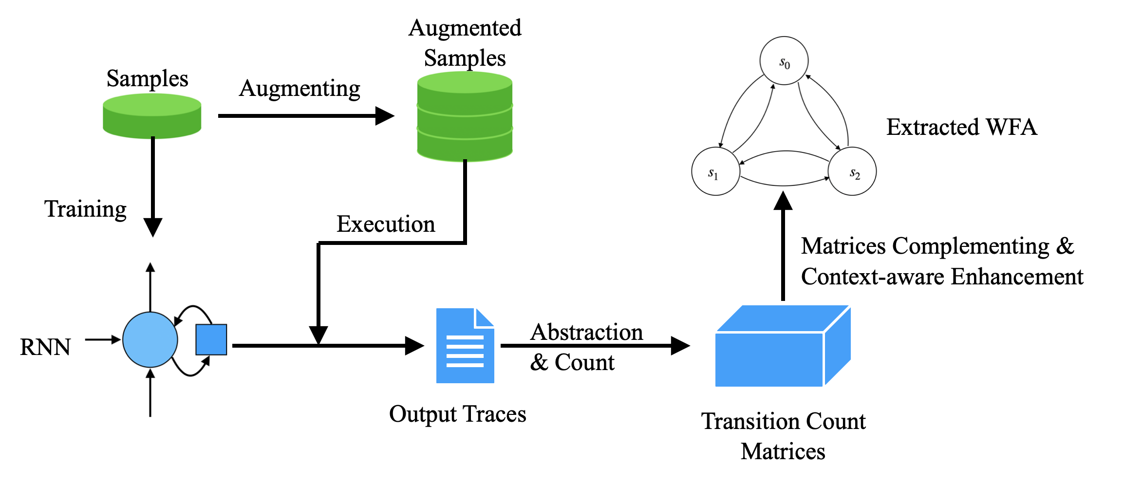
Figure 1: An illustration of our approach to extracting WFA from RNN.

3 Weighted Automata Extraction Scheme

3.1 Outline

We present the workflow of our extraction procedure in Fig. 1. As the first step, we generate augmented sample set ${\mathcal{D}}$ from the original training set $\mathcal{D}_{0}$ to enrich the transition dynamics of RNN behaviors and alleviate the transition sparsity. Then, we execute RNN $\mathcal{R}$ on the augmented sample set ${\mathcal{D}}$, and record the probabilistic output trace $T(w)$ of each input sentence $w\in\mathcal{D}$. With the output set $\hat{O}=\bigcup\limits_{w\in\mathcal{D}}T(w)$, we cluster the probabilistic outputs into abstract states $\hat{S}$, and generate abstract transitions $\mathcal{T}$ from the output traces $\{T(w)|w\in\mathcal{D}\}$. All transitions constitute the abstract transition count matrices $\hat{T}_{\sigma}$ for all $\sigma\in\Sigma$.

Next, we construct the transition matrices $E=\{E_{\sigma}|\sigma\in\Sigma\}$. Based on the abstract states $\hat{S}$ and count matrices $\hat{T}$, we construct the transition matrix $E_{\sigma}$ for each word $\sigma\in\Sigma$. Specifically, we use frequencies to calculate the transition probabilities. Suppose that there are $n$ abstract states in $\hat{S}$. The $i$-th row of $E_{\sigma}$, which indicates the probabilistic transition distribution over states when $\mathcal{R}$ is in state $\hat{s}_{i}$ and consumes $\sigma$, is calculated as

$$E_{\sigma}[i,j]=\frac{\hat{T}_{\sigma}[i,j]}{\sum\limits_{k=1}^{n}\hat{T}_{\sigma}[i,k]}.$$ (1)

This empirical rule faces the problem that the denominator of (1) could be zero, which means that the word $\sigma$ never appears when the RNN $\mathcal{R}$ is in abstract state $\hat{s}_{i}$. In this case, one should decide how to fill in the transition rule of the missing rows in $E_{\sigma}$. In Section 3.2, we present a novel approach for transition rule complement. Further, to preserve more contextual information in the case of transition sparsity, we propose an approach to enhancing the context-aware ability of WFA by adjusting the transition matrices, which is discussed in Section 3.3. Note that our approach is generic and could be applied to other RNNs besides the domain of natural language processing.

3.2 Missing Rows Complementing

Existing approaches for transition rule extraction usually face the problem of transition sparsity, i.e., missing rows in the transition diagram. In the context of formal languages, the probability of occurrence of missing rows is quite limited, since the size of the alphabet is small and each token in the alphabet can appear sufficient number of times. However, in the context of natural language processing, the occurrence of missing rows is quite frequent. The following proposition gives an approximation of the occurrence frequency of missing rows.

Proposition 1

Assume an alphabet $\Sigma$ with $m=|\Sigma|$ words, a natural language dataset $\mathcal{D}$ over $\Sigma$ which has $N$ words in total, a RNN $\mathcal{R}$ trained on $\mathcal{D}$, the extracted abstract states $\hat{S}$ and transitions $\mathcal{T}$. Let $\sigma_{i}$ denote the $i$-th most frequent word occurred in $\mathcal{D}$ and $t_{i}=\mathcal{T}.count((*,\sigma_{i},*))$ indicates the occurrence times of $\sigma_{i}$ in $\mathcal{D}$. The median of $\{t_{i}|1\leq i\leq m\}$ can be estimated as

$$t_{[\frac{m}{2}]}=\frac{2N}{m\cdot\ln m}.$$

Proof

The Zipf’s law [21] shows that

$$\frac{t_{i}}{N}\approx\frac{i^{-1}}{\sum\limits_{k=1}^{m}k^{-1}}.$$

Note that $\sum\limits_{k=1}^{m}k^{-1}\approx\ln m$ and take $i$ to be $\frac{m}{2}$, we complete our proof.

Example 1

In the QC news dataset [16], which has $m=20317$ words in its alphabet and $N=205927$ words in total, the median of $\{t_{i}\}$ is approximated to $\frac{2N}{m\cdot\ln m}\approx 2$. This indicates that about half of $E_{\sigma}$ are constructed with no more than $2$ transitions. In practice, the number of abstract states is usually far more than the transition numbers for these words, making most of rows of their transition matrices missing rows.

Filling the missing row with $\vec{0}$ is a simple solution, since no information were provided from the transitions. However, as estimated above, this solution will lead to the problem of transition sparsity, i.e., the transition matrices for uncommon words are nearly null. Consequently, if the input sequence includes some uncommon words, the weights over states tend to vanish. We refer to this solution as null filling.

Another simple idea is to use the uniform distribution over states for fairness. In [26], the uniform distribution is used as the transition distribution for unseen tokens in the context of formal language tasks. However, for natural language processing, this solution still loses information of the current word, despite that it avoids the weight vanishment over states. We refer to this solution as uniform filling. [29] uses the synonym transition distribution for an unseen token at a certain state. However, it increases the computation overhead when performing inference on test data, since it requires to calculate and sort the distance between the available tokens at a certain state and the unseen token.

To this end, we propose a novel approach to constructing the transition matrices based on two empirical observations. First, each abstract state $\hat{s}\in\hat{S}$ has explicit semantics, i.e. the probabilistic distribution over labels, and similar abstract states tend to share more similar transition behaviours. The similarity of abstract states is defined by their semantic distance as follows.

Definition 3 (State Distance)

For two abstract states $\hat{s}_{1}$ and $\hat{s}_{2}$, the distance between $\hat{s}_{1}$ and $\hat{s}_{2}$ is defined by the Euclidean distance between their center:

$$dist(\hat{s}_{1},\hat{s}_{2})=\lVert\rho(\hat{s}_{1})-\rho(\hat{s}_{2})\rVert_{2}.$$

We calculate the distance between each pair of abstract states, which forms a distance matrix $M$ where each element $M[i,j]=dist(\hat{s}_{i},\hat{s}_{j})$ for $1\leq i,j\leq|\hat{S}|$. For a missing row in $E_{\sigma}$, following the heuristics that similar abstract states are more likely to have similar behaviors, we observe the transition behaviors from other abstract states, and simulate the missing transition behaviors weighted by distance between states. Particularly, in order to avoid numerical underflow, we leverage softmin on distance to bias the weight to states that share more similarity. Formally, for a missing row $E_{\sigma}[i]$, the weight of information set for another row $E_{\sigma}[j]$ is defined by $e^{-M[i,j]}$.

Second, it is also observed that sometimes the RNN just remains in the current state after reading a certain word. Intuitively, this is because part of words in the sentence do not deliver significant information in the task. Therefore, we consider simulating behaviors from other states whilst remaining in the current state with a certain probability.

In order to balance the trade-off between referring to behaviors from other states and remaining still, we introduce a hyper-parameter $\beta$ named reference rate, such that when WFA is faced with a missing row, it has a probability of $\beta$ to refer to the transition behaviors from other states, and in the meanwhile has a probability of $1-\beta$ to keep still. We select the parameter $\beta$ according to the proportion of self-transitions, i.e., transitions $(\hat{s},\sigma,\hat{s}^{\prime})$ in $\mathcal{T}$ where $\hat{s}=\hat{s}^{\prime}$.

To sum up, the complete transition rule for the missing row is

$$E_{\sigma}[i,j]=\beta\cdot\frac{\sum\limits_{k=1}^{n}e^{-M[i,k]}\cdot\hat{T}_{\sigma}[k,j]}{\sum\limits_{l=1}^{n}\sum\limits_{k=1}^{n}e^{-M[i,k]}\cdot\hat{T}_{\sigma}[k,l]}+(1-\beta)\cdot\delta_{i,j}.$$ (2)

Here $\delta_{i,j}$ is the Kronecker symbol:

$$\delta_{i,j}=\begin{cases}1,&j=i\\ 0,&j\neq i\end{cases}.$$

In practice, we can calculate $\sum\limits_{k=1}^{n}e^{-M[i,k]}\cdot\hat{T}_{\sigma}[k,j]$ for each $j$ and then make division on their summation once and for all, which can reduce the computation overhead on transition rule extraction.

3.3 Context-Aware Enhancement

For NLP tasks, the memorization of long-term context information is crucial. One of the advantages of RNN and its advanced design LSTM networks is the ability to capture long-term dependency. We expect the extracted WFA to simulate the step-wise behaviors of RNNs whilst keeping track of context information along with the state transition. To this end, we propose an approach to adjusting the transition matrix such that the WFA can remain in the current state with a certain probability.

Specifically, we select a hyper-parameter $\alpha\in[0,1]$ as the static probability. For each word $\sigma\in\Sigma$ and its transition matrix $E_{\sigma}$, we replace the matrix with the context-aware enhanced matrix $\hat{E}_{\sigma}$ as follows:

$$\hat{E}_{\sigma}=\alpha\cdot I_{n}+(1-\alpha)\cdot E_{\sigma}$$ (3)

where $I_{n}$ is the identity matrix.

The context-aware enhanced matrix has explicit semantics. When the WFA is in state $\hat{s}_{i}$ and ready to process a new word $\sigma$, it has a probability of $\alpha$ (the static probability) to remain in $\hat{s}_{i}$, or follows the original transition distribution $E_{\sigma}[i,j]$ with a probability $1-\alpha$.

Here we present an illustration of how context-aware enhanced matrices deliver long-term context information. Suppose that a context-aware enhanced WFA $\mathcal{A}$ is processing a sentence $w\in\Sigma^{*}$ with length $|w|$. We denote $d_{i}$ as the distribution over all abstract states after $\mathcal{A}$ reads the prefix $w[:i]$, and particularly $d_{0}=I$ is the initial vector of $\mathcal{A}$. We use $Z_{i}$ to denote the decision made by $\mathcal{A}$ based on $d_{i-1}$ and the original transition matrix $E_{w_{i}}$. Formally, $d_{i}=d_{i-1}\cdot\hat{E}_{w_{i}}$ and $Z_{i}=d_{i-1}\cdot E_{w_{i}}$.

The $d_{i}$ can be regarded as the information obtained from the prefix $w[:i]$ by $\mathcal{A}$ before it consumes $w_{i+1}$, and $Z_{i}$ can be considered as the decision made by $\mathcal{A}$ after it reads $w_{i}$.

Proposition 2

The $i$-th step-wise information $d_{i}$ which delivered by processing $w[:i]$ contains the decision information $Z_{j}$ of prefix $w[:j]$ with a proportion of $(1-\alpha)\cdot\alpha^{i-j}$, $1\leq j\leq i$.

Proof

Since $\hat{E}_{w_{i}}=\alpha\cdot I_{n}+(1-\alpha)\cdot E_{w_{i}}$, we can calculate that

$$d_{i}=d_{i-1}\cdot\hat{E}_{w_{i}}=d_{i-1}\cdot[\alpha\cdot I_{n}+(1-\alpha)\cdot E_{w_{i}}]=\alpha\cdot d_{i-1}+(1-\alpha)\cdot Z_{i}.$$ (4)

Using (4) recursively, we have

$$d_{i}=(1-\alpha)\sum_{k=1}^{i}\alpha^{i-k}\cdot Z_{k}+\alpha^{i}\cdot I.$$

This shows the information delivered by $w[:i]$ refers to the decision made by $\mathcal{A}$ on each prefix included in $w[:i]$, and the portion vanishes exponentially. The effectiveness of the context-aware transition matrix adjustment method will be discussed in Section 5.

The following example presents the complete approach for transition rule extraction, i.e., to generate the transition matrix $\hat{E}_{\sigma}$ with the missing row filled in and context enhanced, from the count matrix $\hat{T}_{\sigma}$ for a word $\sigma\in\Sigma$.

Example 2

Assume that there are three abstract states in $\hat{S}=\{\hat{s}_{1},\hat{s}_{2},\hat{s}_{3}\}.$ Suppose the count matrix for $\sigma$ is $\hat{T}_{\sigma}$.

$$\hat{T}_{\sigma}=\begin{bmatrix}1&3&0\\ 1&1&0\\ 0&0&0\end{bmatrix},E_{\sigma}=\begin{bmatrix}0.25&0.75&0\\ 0.5&0.5&0\\ 0.15&0.35&0.5\end{bmatrix},\hat{E}_{\sigma}=\begin{bmatrix}0.4&0.6&0\\ 0.4&0.6&0\\ 0.12&0.28&0.6\end{bmatrix}.$$

For the first two rows (states), there exist transitions for $\sigma$, thus we can calculate the transition distribution of these two rows in $E_{\sigma}$ in the usual way. However, the third row is a missing row. We set the reference rate as $\beta=0.5$, and suppose that the distance between states satisfies $e^{-M[1,3]}=2e^{-M[2,3]}$, generally indicating the distance between $\hat{s}_{1}$ and $\hat{s}_{3}$ is nearer than $\hat{s}_{2}$ and $\hat{s}_{3}$. With the transitions from $\hat{s}_{1}$ and $\hat{s}_{2}$, we can complement the transition rule of the third row in $E_{\sigma}$ through (2). The result shows that the behavior from $\hat{s}_{3}$ is more similar to $\hat{s}_{1}$ than $\hat{s}_{2}$, due to the nearer distance. Finally, we construct $\hat{E}_{\sigma}$ with $E_{\sigma}$. Here we take the static probability $\alpha=0.2$, thus $\hat{E}_{\sigma}=0.2\cdot I_{3}+0.8\cdot E_{\sigma}$. The result shows that the WFA with $\hat{E}_{\sigma}$ has higher probability to remain in the current state after consuming $\sigma$, which can preserve more information from the prefix before $\sigma$.

4 Data Augmentation

Our proposed approach for transition rule extraction provides a solution to the transition sparsity problem. Still, we hope to learn more dynamic transition behaviors from the target RNN, especially for the words with relatively low frequency to characterize their transition dynamics sufficiently based on the finite data samples. Different from formal languages, we can generate more natural language samples automatically, as long as the augmented sequential data are sensible with clear semantics and compatible with the original learning task. Based on the augmented samples, we are able to track more behaviors of the RNN and build the abstract model with higher precision. In this section, we introduce two data augmentation tactics for natural language processing tasks: Synonym Replacement and Dropout.

4.0.1 Synonym Replacement.

Based on the distance quantization among the word embedding vectors, we can obtain a list of synonyms for each word in $\Sigma$. For a word $\sigma\in\Sigma$, the synonyms of $w$ are defined as the top $k$ most similar words of $\sigma$ in $\Sigma$, where $k$ is a hyper-parameter. The similarity among the words is calculated based on the Euclidean distance between the word embedding vectors over $\Sigma$.

Given a dataset $\mathcal{D}_{0}$ over $\Sigma$, for each sentence $w\in\mathcal{D}_{0}$, we generate a new sentence $w^{\prime}$ by replacing some words in $w$ with their synonyms. Note that we hope that the uncommon words in $\Sigma$ should appear more times, so as to gather more dynamic behaviors of RNNs when processing such words. Therefore, we set the probability that a certain word $\sigma\in w$ gets replaced to be in a negative correlation to its frequency of occurrence, i.e. the $i$-th most frequent word is replaced with a probability $\frac{1}{i+1}$.

4.0.2 Dropout.

Inspired by the regularization technique dropout, we also propose a similar tactic to generate new sentences from $\mathcal{D}_{0}$. Initially, we introduce a new word named unknown word and denote it as $\left\langle\textbf{unk}\right\rangle$. For the sentence in $w\in\mathcal{D}_{0}$ that has been processed by synonym replacing, we further replace the words that hasn’t been replaced with $\left\langle\textbf{unk}\right\rangle$ with a certain probability. Finally, new sentences generated by both synonym replacement and dropout form the augmented dataset $\mathcal{D}$.

With the dropout tactic, we can observe the behaviors of RNNs when it processes an unknown word $\hat{\sigma}\not\in\Sigma$ that hasn’t appeared in $\mathcal{D}_{0}$. Therefore, the extracted WFA can also show better generalization ability. An example of generating a new sentence from $\mathcal{D}_{0}$ is shown as follows.

Example 3

Consider a sentence $w$ from the original training set $\mathcal{D}_{0}$, $w=$[“I”, “really”, “like”, “this”, “movie”]. First, the word “like” is chosen to be replaced by one of its synonym “appreciate”. Next, the word “really” is dropped from the sentence, i.e. replaced by the unknown word $\langle\textbf{unk}\rangle$. Finally, we get a new sentence $w^{\prime}=$[“I”, “$\langle\textbf{unk}\rangle$”, “appreciate”, “this”, “movie”] and put it into the augmented dataset $\mathcal{D}$.

Since the word “appreciate” may be an uncommon word in $\Sigma$, we can capture a new transition information for it given by RNNs. Besides, we can also observe the behavior of RNN when it reads an unknown word after the prefix [“I”].

4.0.3 Computational Complexity.

The time complexity of the whole workflow is analyzed as follows. Suppose that the set of training samples $\mathcal{D}_{0}$ has $N$ words in total and its alphabet $\Sigma$ contains $n$ words, and is augmented as $\mathcal{D}$ with $t$ epochs (i.e. each sentence in $\mathcal{D}_{0}$ is transformed to $t$ new sentences in $\mathcal{D}$), hence $|\mathcal{D}|=(t+1)N$. Assume that a probabilistic output of RNNs is a $m$-dim vector, and the abstract states set $\hat{S}$ contains $k$ states.

To start with, the augmentation of $\mathcal{D}_{0}$ and tracking of probabilistic outputs in $\mathcal{D}$ will be completed in $\mathcal{O}(|\mathcal{D}|)=\mathcal{O}(t\cdot N)$ time. Besides, the time complexity of k-means clustering algorithm is $\mathcal{O}(k\cdot|\mathcal{D}|)=\mathcal{O}(k\cdot t\cdot N)$. The count of abstract transitions will be done in $\mathcal{O}(n)$. As for the processing of transition matrices, we need to calculate the transition probability for each word $\sigma$ with each source state $\hat{s}_{i}$ and destination state $\hat{s}_{j}$, which costs $\mathcal{O}(k^{2}\cdot n)$ time. Finally, the context-aware enhancement on transition matrices takes $\mathcal{O}(k\cdot n)$ time.

Note that $\mathcal{O}(n)=\mathcal{O}(N)$, hence we can conclude that the time complexity of our whole workflow is $\mathcal{O}(k^{2}\cdot t\cdot N)$. So the time complexity of our approaches only takes linear time w.r.t. the size of the dataset, which provides theoretical extraction overhead for large-scale data applications.

5 Experiments

In this section, we evaluate our extraction approach on two natural language datasets and demonstrate its performance in terms of precision and scalability.

Datasets and RNNs models.

We select two popular datasets for NLP tasks and train the target RNNs on them.

1. The CogComp QC Dataset (abbrev. QC) [16] contains news titles which are labeled with different topics. The dataset is divided into a training set containing 20k samples and a test set containing 8k samples. Each sample is labeled with one of seven categories. We train an LSTM-based RNN model $\mathcal{R}$ on the training set, which achieves an accuracy of $81\%$ on the test set.

2. The Jigsaw Toxic Comment Dataset (abbrev. Toxic) [15] contains comments from Wikipedia’s talk page edits, with each comment labeled toxic or not. We select 25k non-toxic samples and toxic samples respectively, and divide them into the training set and test set in a ratio of four to one. We train another LSTM-based RNN model which achieves $90\%$ accuracy.

Metrics.

For the purpose of representing the behaviors of RNNs better, we use Consistency Rate (CR) as our evaluation metric. For a sentence in the test set $w\in\mathcal{D}_{test}$, we denote $\mathcal{R}(w)$ and $\mathcal{A}(w)$ as the prediction results of the RNNs and WFA, respectively. The Consistency Rate is defined formally as

$$CR=\frac{|\{w\in D_{test}:\mathcal{A}(w)=\mathcal{R}(w)\}|}{|\mathcal{D}_{test}|}.$$

5.0.1 Missing Rows Complementing.

As discussed in Section 3.2, we take two approaches as baselines, the null filling and the uniform filling. The two WFA extracted with these two approaches are denoted as $\mathcal{A}_{0}$ and $\mathcal{A}_{U}$, respectively. The WFA extracted by our empirical filling approach is denoted as $\mathcal{A}_{E}$.

Table 1: Evaluation results of different filling approaches on missing rows.

Dataset	$\mathcal{A}_{0}$		$\mathcal{A}_{U}$		$\mathcal{A}_{E}$
	CR(%)	Time(s)	CR(%)	Time(s)	CR(%)	Time(s)
QC	26	47	60	56	80	70
Toxic	57	167	86	180	91	200

Table 1 shows the evaluation results of three rule filling approaches. We conduct the comparison experiments on QC and Toxic datasets and select the cluster number for state abstraction as $40$ and $20$ for the QC and Toxic datasets, respectively.

The three columns labeled with the type of WFA show the evaluation results of different approaches. For the $\mathcal{A}_{0}$ based on blank filling, the WFA returns the weight of most sentences in $\mathcal{D}$ with $\vec{0}$, which fails to provide sufficient information for prediction. For the QC dataset, only a quarter of sentences in the test set are classified correctly. The second column shows that the performance of $\mathcal{A}_{U}$ is better than $\mathcal{A}_{0}$. The last column presents the evaluation result of $\mathcal{A}_{E}$, which fills the missing rows by our approach. In this experiment, the hyper-parameter reference rate is set as $\beta=0.3$. We can see that our empirical approach achieves significantly better accuracy, which is $20\%$ and $5\%$ higher than uniform filling on the two datasets, respectively.

The columns labeled Time show the execution time of the whole extraction workflow, from tracking transitions to evaluation on test set, but not include the training time of RNNs. We can see that the extraction overhead of our approach ($\mathcal{A}_{E}$) is about the same as $\mathcal{A}_{U}$ and $\mathcal{A}_{0}$.

5.0.2 Context-Aware Enhancement.

In this experiment, we leverage the context-aware enhanced matrices when constructing the WFA. We adopt the same configuration on cluster numbers $n$ from the comparison experiments above, i.e. $n=40$ and $n=20$. The columns titled Configuration indicate if the extracted WFA leverage context-aware matrices. We also take the WFA with different filling approaches, the uniform filling and empirical filling, into comparison. Experiments on null filling is omitted due to limited precision.

Table 2: Evaluation results of with and without context-aware enhancement.

Dataset	Configuration	$\mathcal{A}_{U}$		$\mathcal{A}_{E}$
		CR(%)	Time(s)	CR(%)	Time(s)
QC	None	60	56	80	70
	Context	71	64	82	78
Toxic	None	86	180	91	200
	Context	89	191	92	211

The experiment results are in Table 2. For the QC dataset, we set the static probability as $\alpha=0.4$. The consistency rate of WFA $\mathcal{A}_{U}$ improves $11\%$ with the context-aware enhancement, and $\mathcal{A}_{E}$ improves $2\%$. As for the Toxic dataset, we take $\alpha=0.2$ and the consistency rate of the two WFA improves $3\%$ and $1\%$ respectively. This shows that the WFA with context-aware enhancement remains more information from the prefixes of sentences, making it simulate RNNs better.

Still, the context-aware enhancement processing costs little time, since we only calculate the adjusting formula (3) for each $E_{\sigma}$ in $E$. The additional extra time consumption is 8s for the QC dataset and 11s for the Toxic dataset.

5.0.3 Data Augmentation

Finally, we evaluate the WFA extracted with transition behaviors from augmented data. Note that the two experiments above are based on the primitive training set $\mathcal{D}_{0}$. In this experiment, we leverage the data augmentation tactics to generate the augmented training set $\mathcal{D}$, and extract WFA with data samples from $\mathcal{D}$. In order to get best performance, we build WFA with contextual-aware enhanced matrices.

Table 3: Evaluation results of with and without data augmentation.

Dataset	Samples	$\mathcal{A}_{U}$		$\mathcal{A}_{E}$
		CR(%)	Time(s)	CR(%)	Time(s)
QC	$\mathcal{D}_{0}$	71	64	82	68
	$\mathcal{D}$	76	81	84	85
Toxic	$\mathcal{D}_{0}$	89	191	92	211
	$\mathcal{D}$	91	295	94	315

Table 3 shows the results of consistency rate of WFA extracted with and without augmented data. The rows labeled $\mathcal{D}_{0}$ show the results of WFA that are extracted with the primitive training set, and the result from the augmented data is shown in rows labeled $\mathcal{D}$. With more transition behaviors tracked, the WFA extracted with $\mathcal{D}$ demonstrates better precision. Specifically, the WFA extracted with both empirical filling and context-aware enhancement achieves a further $2\%$ increase in consistency rate on the two datasets.

To summarize, by using our transition rule extraction approach, the consistency rate of extracted WFA on the QC dataset and the Toxic dataset achieves $84\%$ and $94\%$, respectively. Taking the primitive extraction algorithm with uniform filling as baseline, of which experimental results in terms of CR are $60\%$ and $86\%$, our approach achieves an improvement of $22\%$ and $8\%$ in consistency rate. As for the time complexity, the time consumption of our approach increases from $56s$ to $81s$ on QC dataset, and from $180s$ to $315s$ on Toxic dataset, which indicates the efficiency and scalability of our rule extraction approach. There is no significant time cost of adopting our approach further for complicated natural language tasks. We can conclude that our transition rule extraction approach makes better approximation of RNNs, and is also efficient enough to be applied to practical applications for large-scale natural language tasks.

6 Related Work

Many research efforts have been made to abstract, verify and repair RNNs. As Jacobsson reviewed in [14], the rule extraction approach of RNNs can be divided into two categories: pedagogical approaches and compositional approaches.

Pedagogical Approaches.

Much progress has been achieved by using pedagogical approaches to abstracting RNNs by leveraging explicit learning algorithms, such as the $L^{*}$ algorithm [2]. The earlier work dates back to two decades ago, when Omlin et al. attempted to extract a finite model from Boolean-output RNNs [20, 18, 19]. Recently, Weiss et al. proposed to levergae the $L^{*}$ algorithm to extract DFA from RNN-acceptors [25]. Later, they presented a weighted extension of $L^{*}$ algorithm that extracted probabilistic determininstic finite automata (PDFA) from RNNs [26]. Besides, Okudono et al. proposed another weighted extension of $L^{*}$ algorithm to extract WFA from real-value-output RNNs [17].

The pedagogical approaches have achieved great success in abstracting RNNs for small-scale languages, particularly formal languages. Such exact learning approaches have intrinsic limitation in the scalability of the language complexity, hence they are not suitable for automata extraction from natural language processing models.

Compositional Approach.

Another technical line is the compositional approach, which generally leverages unsupervised algorithms (e.g. k-means, GMM) to cluster state vectors as abstract states [28, 4]. Wang et al. studied the key factors that influence the reliability of extraction process, and proposed an empirical rule to extract DFA from RNNs [23]. Later, Zhang et al. followed the state encoding of compositional approach and proposed a WFA extraction approach from RNNs [29], which can be applied to both grammatical languages and natural languages. In this paper, our proposal of extracting WFA from RNNs also falls into the line of compositional approach, but aims at proposing transition rule extraction method to address the transition sparsity problem and enhance the context-aware ability.

Recently, many of the verification, analysis and repairment works also leverage similar approaches to abstract RNNs as a more explicit model, such as DeepSteller [9], Marble [8] and RNNsRepair [27]. These works achieve great progress in analyzing and repairing RNNs, but have strict requirements of scalability to large-scale tasks, particularly natural language processing. The proposed approach, which demonstrates better precision and scalability, shows great potential for further applications such as RNN analysis and Network repairment. We consider applying our method to RNN analysis as future work.

7 Conclusion

This paper presents a novel approach to extracting transition rules of weighted finite automata from recurrent neural networks. We measure the distance between abstract states and complement the transition rules of missing rows. In addition, we present an heuristic method to enhance the context-aware ability of the extracted WFA. We further propose two augmentation tactics to track more transition behaviours of RNNs. Experiments on two natural language datasets show that the WFA extracted with our approach achieve better consistency with target RNNs. The theoretical estimation of computation complexity and experimental results demonstrate that our rule extraction approach can be applied to natural language datasets and complete the extraction procedure efficiently for large-scale tasks.

7.0.1 Acknowledgements

This research was sponsored by the National Natural Science Foundation of China under Grant No. 62172019, 61772038, and CCF-Huawei Formal Verification Innovation Research Plan.

References

- [1] Abdel-Hamid, O., Mohamed, A.r., Jiang, H., Deng, L., Penn, G., Yu, D.: Convolutional neural networks for speech recognition. IEEE/ACM Transactions on audio, speech, and language processing 22(10), 1533–1545 (2014)
- [2] Angluin, D.: Learning regular sets from queries and counterexamples. Information and computation 75(2), 87–106 (1987)
- [3] Baier, C., Katoen, J.P.: Principles of model checking. MIT press (2008)
- [4] Cechin, A.L., Regina, D., Simon, P., Stertz, K.: State automata extraction from recurrent neural nets using k-means and fuzzy clustering. In: 23rd International Conference of the Chilean Computer Science Society, 2003. SCCC 2003. Proceedings. pp. 73–78. IEEE (2003)
- [5] Che, Z., Purushotham, S., Cho, K., Sontag, D., Liu, Y.: Recurrent neural networks for multivariate time series with missing values. Scientific reports 8(1), 1–12 (2018)
- [6] Datta, D., David, P.E., Mittal, D., Jain, A.: Neural machine translation using recurrent neural network. International Journal of Engineering and Advanced Technology 9(4), 1395–1400 (2020)
- [7] Dong, G., Wang, J., Sun, J., Zhang, Y., Wang, X., Dai, T., Dong, J.S., Wang, X.: Towards interpreting recurrent neural networks through probabilistic abstraction. In: 2020 35th IEEE/ACM International Conference on Automated Software Engineering (ASE). pp. 499–510. IEEE (2020)
- [8] Du, X., Li, Y., Xie, X., Ma, L., Liu, Y., Zhao, J.: Marble: Model-based robustness analysis of stateful deep learning systems. In: Proceedings of the 35th IEEE/ACM International Conference on Automated Software Engineering. pp. 423–435 (2020)
- [9] Du, X., Xie, X., Li, Y., Ma, L., Liu, Y., Zhao, J.: Deepstellar: Model-based quantitative analysis of stateful deep learning systems. In: Proceedings of the 2019 27th ACM Joint Meeting on European Software Engineering Conference and Symposium on the Foundations of Software Engineering. pp. 477–487 (2019)
- [10] Gastin, P., Monmege, B.: A unifying survey on weighted logics and weighted automata. Soft Computing 22(4), 1047–1065 (2018)
- [11] Goldberg, Y.: Neural network methods for natural language processing. Synthesis lectures on human language technologies 10(1), 1–309 (2017)
- [12] He, K., Zhang, X., Ren, S., Sun, J.: Deep residual learning for image recognition. In: Proceedings of the IEEE Conference on Computer Vision and Pattern Recognition (CVPR) (June 2016)
- [13] Hochreiter, S., Schmidhuber, J.: Long short-term memory. Neural computation 9(8), 1735–1780 (1997)
- [14] Jacobsson, H.: Rule extraction from recurrent neural networks: Ataxonomy and review. Neural Computation 17(6), 1223–1263 (2005)
- [15] Jigsaw: Toxic comment classification challenge, https://www.kaggle.com/c/jigsaw-toxic-comment-classification-challenge Accessed April 16, 2022
- [16] Li, X., Roth, D.: Learning question classifiers. In: COLING 2002: The 19th International Conference on Computational Linguistics (2002)
- [17] Okudono, T., Waga, M., Sekiyama, T., Hasuo, I.: Weighted automata extraction from recurrent neural networks via regression on state spaces. In: Proceedings of the AAAI Conference on Artificial Intelligence. vol. 34, pp. 5306–5314 (2020)
- [18] Omlin, C.W., Giles, C.L.: Extraction of rules from discrete-time recurrent neural networks. Neural networks 9(1), 41–52 (1996)
- [19] Omlin, C.W., Giles, C.L.: Rule revision with recurrent neural networks. IEEE Transactions on Knowledge and Data Engineering 8(1), 183–188 (1996)
- [20] Omlin, C., Giles, C., Miller, C.: Heuristics for the extraction of rules from discrete-time recurrent neural networks. In: [Proceedings 1992] IJCNN International Joint Conference on Neural Networks. vol. 1, pp. 33–38. IEEE (1992)
- [21] Powers, D.M.: Applications and explanations of zipf’s law. In: New methods in language processing and computational natural language learning (1998)
- [22] Wang, Q., Zhang, K., Liu, X., Giles, C.L.: Verification of recurrent neural networks through rule extraction. arXiv preprint arXiv:1811.06029 (2018)
- [23] Wang, Q., Zhang, K., Ororbia II, A.G., Xing, X., Liu, X., Giles, C.L.: An empirical evaluation of rule extraction from recurrent neural networks. Neural computation 30(9), 2568–2591 (2018)
- [24] Wang, R., Li, Z., Cao, J., Chen, T., Wang, L.: Convolutional recurrent neural networks for text classification. In: 2019 International Joint Conference on Neural Networks (IJCNN). pp. 1–6. IEEE (2019)
- [25] Weiss, G., Goldberg, Y., Yahav, E.: Extracting automata from recurrent neural networks using queries and counterexamples. In: International Conference on Machine Learning. pp. 5247–5256. PMLR (2018)
- [26] Weiss, G., Goldberg, Y., Yahav, E.: Learning deterministic weighted automata with queries and counterexamples. In: Wallach, H., Larochelle, H., Beygelzimer, A., d'Alché-Buc, F., Fox, E., Garnett, R. (eds.) Advances in Neural Information Processing Systems. vol. 32. Curran Associates, Inc. (2019), https://proceedings.neurips.cc/paper/2019/file/d3f93e7766e8e1b7ef66dfdd9a8be93b-Paper.pdf
- [27] Xie, X., Guo, W., Ma, L., Le, W., Wang, J., Zhou, L., Liu, Y., Xing, X.: Rnnrepair: Automatic rnn repair via model-based analysis. In: International Conference on Machine Learning. pp. 11383–11392. PMLR (2021)
- [28] Zeng, Z., Goodman, R.M., Smyth, P.: Learning finite state machines with self-clustering recurrent networks. Neural Computation 5(6), 976–990 (1993)
- [29] Zhang, X., Du, X., Xie, X., Ma, L., Liu, Y., Sun, M.: Decision-guided weighted automata extraction from recurrent neural networks. In: Thirty-Fifth AAAI Conference on Artificial Intelligence (AAAI). pp. 11699–11707. AAAI Press (2021)