On the Prediction Network Architecture in RNN-T for ASR

Abstract

RNN-T models have gained popularity in the literature and in commercial systems because of their competitiveness and capability of operating in online streaming mode. In this work, we conduct an extensive study comparing several prediction network architectures for both monotonic and original RNN-T models. We compare 4 types of prediction networks based on a common state-of-the-art Conformer encoder and report results obtained on Librispeech and an internal medical conversation data set. Our study covers both offline batch-mode and online streaming scenarios. In contrast to some previous works, our results show that Transformer does not always outperform LSTM when used as prediction network along with Conformer encoder. Inspired by our scoreboard, we propose a new simple prediction network architecture, $N$-Concat, that outperforms the others in our online streaming benchmark. Transformer and n-gram reduced architectures perform very similarly yet with some important distinct behaviour in terms of previous context. Overall we obtained up to 4.1 % relative WER improvement compared to our LSTM baseline, while reducing prediction network parameters by nearly an order of magnitude (8.4 times).

Index Terms: Conformer, RNN-T, prediction network, online, MHSA, Transformer

1 Introduction

Recurrent Neural Network Transducer (RNN-T) [1] was proposed as an extension to Connectionist Temporal Classification (CTC) [2] by relaxing CTC’s assumption of conditional label independence between predictions given the audio. In addition to the CTC acoustic encoder, RNN-T introduced a prediction network (PN) and a joiner network. The PN autoregressively incorporates previously emitted tokens into the model, while the joiner mixes both acoustic and autoregressive label representations via a monotonic alignment process. Some extensions were proposed to the original RNN-T loss including HAT [3], RNA [4], and in particular MonoRNN-T [5] which constrains the number of output tokens per acoustic input frame in RNN-T alignments. Significant architectural improvements have been proposed since the original RNN-T conception. LSTM/BLSTM were replaced by Transformer [6, 7, 8], and later encoder networks were extended with convolutions in the Conformer [9] and ContextNet [10] architectures. In all cases, for streaming recognition the encoder is bound to real-time application requirements. These requirements restrict the future context, which leads to an encoder induced latency (EIL), that the encoder can exploit. Online encoders generally underperform their offline counterparts because of their limited access to future context. Consequently, many approaches were proposed for better leveraging their scarce EIL [7, 11, 12]. Unfortunately, all approaches deemed future context (aka lookahead) as the critical factor.

Despite the PN being a core RNN-T differentiator, there is a lack of deep understanding of its role. Some works show that the PN plays a language modeling role [3, 13, 14] while others challenge this interpretation [15, 16, 17]. Under some circumstances, the autoregressive dependence of the PN was dramatically simplified to a bigram [15, 8, 18], and even a randomly initialized PN was not significantly detrimental to RNN-T performance for some tasks [17]. Furthermore, there is a full-fledged research line attempting to match RNN-T performance with non-autoregressive CTC-based techniques [16, 19], by dropping the PN and embedding some larger hidden contextual (possibly token) information into the encoder. For this reason, the autoregressive context dependence of some specific PN architectures, such as the Transformer-Transducer (T-T) or the Tied & Reduced (T&R) was analyzed [7, 18]. For instance,  [7] could achieve similar accuracy by limiting left context to 3 tokens, though observed about 5% relative degradation when further reducing it to 2 tokens. N-gram PN was proposed and studied within a causal online Conformer RNN-T encoder [18].

This work is devoted to a systematic study of several PNs under various conditions. While some partial explorations have been done in the literature, we conduct a clean comparison of several PNs together with a common state-of-the-art Conformer encoder, namely: LSTM [20], Transformer [21], Conformer [9], and n-gram reduced [18]. Inspired by [18], we propose a new n-gram PN that outperforms all the other PNs in online configurations on both the Librispeech 100 hour subset and an internal medical data set consisting of 1000 hours of doctor-patient conversations. Motivated by gaining better understanding of the encoder and PN interactions, we assess the PNs in two different regimes, streaming and batch recognition, as well as with character and word-piece vocabularies. We further consider the implications of using either monotonic or original RNN-T loss within this scoreboard. Finally, we study the behavior of the best PNs with limited autoregressive context.

2 RNN-T

Let $x_{1}^{T}=(x_{1},...,x_{T})$ be an input sequence of length $T$, where $x_{t}\in\mathbb{R}^{d}$ is an acoustic feature vector. As originally introduced in  [1], a RNN-T maps $x_{1}^{T}$ to an output token sequence $y_{1}^{U}=(y_{1},\ldots,y_{U})$ of length $U$, where $y_{u}\in\mathcal{Y}$ is an output token and $\mathcal{Y}$ is the vocabulary. This is done via aligning the internal acoustic and token representations. We denote an alignment of length $K=T^{\prime}+U$ as $z_{1}^{K}=(z_{1},\ldots,z_{K})$, where $z_{k}$ belongs to $\mathcal{Y}$ extended with a blank symbol $\epsilon$. $\mathcal{B}^{-1}(y_{1}^{U})$ is the set of all alignments that generate token sequence $y_{1}^{U}$ after removing all blank tokens. Note we have to take into account 3 different lengths, namely, $T$ as original input length, $T^{\prime}$ as encoder output length, and $U$ as label output length (without blank symbol). RNN-T models are composed of 3 components: first the encoder network projects the input acoustics to hidden encoder states $e_{t}=\operatorname{enc}(x_{1}^{T})$ ($T^{\prime}<=T$) for $t=1,\ldots,T^{\prime}$; second the prediction network (PN) autoregressively builds a hidden representation of the previous output tokens $s_{u}=\operatorname{pred}(y_{1}^{u})$ for $u=1,\ldots,U$; and finally the joiner network harmonizes both lengths by reading the encoder representation at $t_{k}$ and the PN representation at $u_{k}$ to generate the alignment output distribution, $p(z_{k}\mid e_{t_{k}},s_{u_{k}})$, over the extended vocabulary. RNN-T models are optimized to minimize the log-likelihood loss over all possible alignments

$$\mathcal{L}=\log p(y_{1}^{U}\mid x_{1}^{T})=\log\sum_{z_{1}^{K}\in\mathcal{B}^{-1}(y_{1}^{U})}p(z_{1}^{K}\mid x_{1}^{T})$$ (1)

with the alignment probability decomposed left-to-right as

$$\textstyle p(z_{1}^{K}\mid x_{1}^{T}):=\prod_{k=1}^{K}p(z_{k}\mid e_{t_{k}},s_{u_{k}})$$ (2)

where $t_{k}$ is obtained by counting the number of blanks in the alignment until $k$ and $u_{k}$ is obtained by counting the number of non-blanks generated until $k$.

As alluded in section 1, two RNN-T variants are analyzed in this work. The original RNN-T model [1] allows alignments with consecutive token sequences without interleaved blanks. In contrast, monotonic RNNT [3, 5] requires incrementing the encoder position $t_{k}$ for each token the PN predicts. In this case, the full alignment length $K$ is $T^{\prime}$ and $t_{k}:=k$ in eq. (2).

2.1 Online Encoder

Our study of different types of PNs in RNN-T covers both offline batch-mode and online streaming scenario. In the online streaming case, the multi-head self-attention (MHSA) and convolutional block in the Conformer encoder have to be constrained in accessing future context because of the latency requirement. The MHSA block can exploit future context, which is determined by the latency requirement for a specific application, in several ways according to the literature: autoregressive [18], truncated look-ahead [6], contextual look-ahead [12] and chunked attention [11]. We conducted experiments with these approaches under the baseline LSTM PN and found that the chunked attention [11] provides the best trade-off (see section 3.1) between latency and accuracy. Therefore, we use this approach, along with causal depth-wise convolutions in the convolutional block, to evaluate different PNs in the online scenario.

2.2 Prediction Networks (PN)

In this work, we mainly compare 4 standard PNs: LSTM, Transformer, Conformer, and n-gram. The LSTM PN consists of one layer unidirectional LSTM [20] to model the full left context, although some research has exploited limited left context  [22]. For the Transformer PN, the MHSA is autoregressively masked with limited left context. For the Conformer PN [9], causal convolutions and MHSA blocks were used in a similar way as in the Transformer case. In the next subsection, we describe n-gram PN, specifically the N-Avg [18] as well as our proposed N-Concat extension in more detail.

2.2.1 Reduced n-gram encoder

N-Avg : Tied and reduced PN [18] simplifies the autoregressive dependency to an n-gram dependency. The previous $N-1$ tokens are used to generate the $s_{u_{k}}$ embedding representation. First, a shared embedding matrix projects each previous token $y_{u-n}$ into a $D$-dimensional embedding vector $v_{u-n}$. Next, the embedding vectors, $v_{u-n}$, are scaled by the dot product between themselves and the positional encodings, $q_{n,h}$, for each head; and then averaged across the full $N$ left context positions and $H$ heads. Finally, a feed-forward neural-network is applied to the averaged representation. Specifically, the PN state $s_{u}$ at $u$, which is used to predict $y_{u+1}$, is computed as

$$s_{u}:=\operatorname{LayerNorm}(\operatorname{Projection}(s_{u}^{(\text{avg})}))$$ (3)

with

$$\textstyle s_{u}^{(\text{avg})}:=\frac{1}{H}\sum_{h=1}^{H}\frac{1}{N}\sum_{n=0}^{N-2}[v_{u-n}\odot q_{h,n}]\cdot v_{u-n}$$ (4)

where $\odot$ is the dot product and $\cdot$ is a scalar-to-vector multiplication.

N-Concat: N-Avg averages along heads and the context tokens. In order to promote an explicit bias towards attending different context tokens, we propose a new variant, N-Concat, that incorporates concatenation heads instead of averaging heads, analogous to standard MHSA [21]. This newly proposed PN allows retention of compressed information from each context token in the final representation. This PN splits the embedding dimension $D$ into $H$ vectors along which it applies a single averaging head from N-Avg. Let $s_{u}(m)$ denote the $m$-th split of the embedding dimension, N-Concat computes

$$\textstyle s_{u}^{(\text{concat})}(m):=\frac{1}{N}\sum_{n=0}^{N-2}[v_{u-n}(m)\odot q_{n}(m)]\cdot v_{u-n}(m)$$ (5)

and then concatenates each into the pre-projected representation

$$\textstyle s_{u}^{(\text{concat})}=(s_{u}^{(\text{concat})}(1),s_{u}^{(\text{concat})}(2),\ldots,s_{u}^{(\text{concat})}(D/H))$$ (6)

Similar to N-Avg, a LayerNorm and Projection is applied to the concatenated representation, $s_{u}^{(\text{concat})}$.

3 Experiments

Table 1: Baseline WER results with Conformer encoder and LSTM PN with various online MHSA configurations for character-based LS100. LA stands for lookahead.

Encoder	EIL	test-clean	test-other
Ours Offline	n.a.	$\mathbf{5.9}$	$\mathbf{16.9}$
chk + causal convs	n.a.	$6.0$	$17.3$
auto-regressive	0.04	$9.2$	$25.4$
chk + 0.96s LA	1.00	$7.6$	$22.6$
chunked (0.5s)	0.52	$7.6$	$22.3$
chk + 0.5s LA	1.00	$7.1$	$21.5$
chk + 0.5s contextual LA	1.00	$\mathbf{6.8}$	$\mathbf{20.4}$
chunked (1s)	1.02	$7.3$	$21.5$

We conducted our experiments on two datasets, Librispeech and an internal medical dataset, using different PNs. In both cases, we extracted 80-channel filterbank features computed from a 25ms window with a stride of 10ms, followed by SpecAugment [23] (without time warping) and finally a small front-end consisting of 2 convolutional layers that perform downsampling by a factor of 4. In all cases, we used Adam [24] and warming-up learning rate schedule [21] tuned as described below. Similarly, we kept the same Conformer encoder architecture [9] while varying the PN.

For the Librispeech corpus [25], we selected the 100 hour training subset (denoted as LS100), and mitigated overfitting by augmenting the data by a factor of 3 with speed perturbation [26] factors in the range of {0.9, 1.0, 1.1}. We used 2 different output token sets: 30 characters and 300 word-pieces with an average length of $4.78$ characters. All models were trained for 100 epochs on the augmented LS100 data set. The training hyperparameters were tuned based on the offline model with Conformer encoder and an LSTM PN using a limited grid search on the clean development set of LS100, then applied to all other models. For assessing the PNs, we used an encoder of 18 Conformer blocks with hidden size of 256, feed-forward (FF) dimension 1024, convolutional kernel width of 15 and 4 attention heads, followed by a joint network of two 256-dimension FF layers with ReLu activation. For the PN, we used a baseline LSTM PN of 256 hidden units; a Transformer PN with 256 hidden dimension, 1024 FF dimension, and 4 heads; a Conformer PN with the same size as the transformer PN plus a convolutional kernel width of 15 tokens; and finally for both n-gram PNs (see section 2.2.1) we used 4 heads followed by a dense layer of 256. All PNs have a single layer since we found them to outperform deeper ones in preliminary experiments, in contrast to some works [6, 7, 8, 16].

Table 2: WER on LS100 varying the PN in offline RNN-T models

PN	output units	test-clean	test-other
LSTM [16]	word-pieces	$6.8$	$18.9$
LSTM (ours)	word-pieces	$6.1$	$16.9$
LSTM	characters	$5.9$	$16.9$
Transformer	characters	$\mathbf{5.6}$	$16.9$
Conformer	characters	$5.7$	$\mathbf{16.4}$
N-Avg	characters	$\mathbf{5.6}$	$16.5$
N-Concat	characters	$5.7$	$16.9$

Additionally, we studied different configurations on an internal medical speech transcription task of doctor-patient conversations (D2P1K), across multiple medical specialties. We use a lab setup where models were trained on 1k hours with a 2.5k word-piece vocabulary of $6.2$ average character length. Word error rate (WER) was computed on a speaker-independent test set consisting of 263k words in total . We tuned the hyperparameters based on the offline LSTM PN baseline, then applied them to the proposed configurations without further tuning. In this case, we used larger and shallower Conformer encoder of 16 blocks with hidden size of 512, FF dimension of 1024, 8 heads and convolutional kernel width of 17 followed by the same joint network as in LS100. Similarly we used larger PN: the LSTM PN baseline is enlarged to 640 hidden units; the Transformer PN is expanded to 640 hidden dimension, 1024 FF dimension, and 8 heads; the Conformer PN uses on top of the transformer PN a convolutional kernel width of 17 tokens; and finally in both n-gram PNs the dense layer is increased to 640 units. We also observed that a single layer PN performed the best in this case. For instance, a 2 layer Transformer PN degraded by 3 % relative WER; and a $2$ layer N-concat by 1%.

3.1 Results With Different Online Approaches in Encoder

Table 1 reports the results with the different online encoder approaches described in section 2.1 with LSTM PN. The contextual look-ahead encoder gave the best accuracy, but at the expense of twice inference time. Conversely, the 1 sec chunked attention encoder offered a competitive trade-off. Based on these results, we use the 1 sec chunked attention in the Conformer encoder in the following study. Note that online models degrade more significantly under adverse acoustic conditions and/or domain mismatch as showed in the results on test-other set.

Table 3: WER on LS100 tests sets for online models with 1 second chunked encoder trained with two output units: characters and word-pieces. PN parameters are reported as # params.

Output label		characters		word-pieces
PN	# params	clean	other	clean	other
LSTM	$0.59$M	$7.3$	$\mathbf{21.5}$	$7.3$	$21.5$
Transformer	$0.9$M	$\mathbf{7.1}$	$22.1$	$7.4$	$22.0$
Conformer	$1.6$M	$7.3$	$21.8$	$7.5$	$21.9$
N-Avg	$0.09$M	$\mathbf{7.1}$	$21.9$	$7.3$	$21.3$
N-Concat	$0.07$M	$\mathbf{7.1}$	$21.9$	$\mathbf{7.0}$	$\mathbf{21.2}$

3.2 Results With Different Prediction Networks (PNs)

Table 2 reports offline results with different PNs on the LS100 dataset with characters as outputs. The results show that the N-Concat performs slightly worse than N-Avg, but better than the LSTM, and competitive with the Transformer and Conformer PN. We also include the corresponding results from  [16] and our LSTM PN result with word-piece units in the table, because our Conformer encoder and LSTM PN have similar configurations as theirs. Note our baseline model is competitive with theirs.

Table 3 reports results from different PNs based on the online Conformer encoder with 1 second chunked-attention. Results are on the LS100 set with both character and word-piece units. For all PN except LSTM, we limit the left context to $5$ word-pieces or $24$ characters, so that a similar amount of context (the average word-piece length is $4.78$ characters) is accessed in both cases. It shows a different picture to that of offline encoders in Table 2. N-Concat works best across the board, while the Conformer PN increases the number of parameters without providing any improvement. The LSTM PN is competitive on test-other with character units, but lags behind on test-clean. The Transformer PN is competitive only on test-clean and only with character units, probably due to the large number of parameters. Both N-Avg and N-Concat perform the same with character units, but N-Concat outperforms N-Avg by 4.1% relative WER reduction with word-pieces while also reducing the number of parameters by 22.5% (or $8.4$ times with respect to the LSTM PN).

In Table 4, different PNs are evaluated on the D2P1K task. Overall, a similar picture to that of LS100 is observed. While the LSTM PN is competitive in offline case, it clearly lags behind in the online case where the performance of different PNs vary significantly. In the online case, N-Concat performs best, though not far from N-Avg and Transformer PN. We hypothesize that the encoder attempts to model the entire transduction task by itself and the PN mainly complements it for disambiguation when conditions become adverse. At the same time, the token prediction task is perhaps learnt faster and consequently a strong model with a long left context dependency is detrimental for generalization because of sparse statistics.

Table 4: WER for different PNs in both offline and online encoder regimes for RNN-T models on D2P1K corpus

PN	Num. PN params	WER
		Offline	Online
LSTM	$3.69$ M	$13.2$	$14.6$
Transformer	$3.78$ M	$\mathbf{12.9}$	$13.9$
Conformer	$5.10$ M	$\mathbf{12.9}$	$14.0$
N-Avg	$0.42$ M	$\mathbf{12.9}$	$13.9$
N-Concat	$0.41$ M	$13.0$	$\mathbf{13.8}$

Table 5: WER and RTF with different PNs for online Monotonic RNN-T on D2P1K. Arrows point to improvement direction. Benchmarked on V100 GPU.

	LSTM	Transf.	Conf.	N-Avg	N-Concat
WER$\downarrow$	$14.2$	$\mathbf{14.1}$	$\mathbf{14.1}$	$14.3$	$14.2$
RTF$\downarrow$	$1.22$	$1.18$	$1.23$	$1.18$	$\mathbf{1.17}$
BS$\uparrow$	$2.5$K	$2.4$K	$2.2$K	$2.5$K	$\mathbf{2.6}$K

Finally, in Table 5, we assess the effects of adding the monoRNN-T constraint to the loss in the online setup. We also report the real time factor (RTF) measured with 3K utterances as batch size in greedy decoding and the maximum batch size at 1 RTF (BS row). Note that the RTF numbers are measured via forward propagating through the whole network. Since the encoder, which contains 64M parameters, dominates in size, the overall RTFs look similar, despite significant reduction in N-Avg and N-Concat PN size. We use 5-gram left context for all but LSTM. Accuracy slightly degrades with respect to Table 4. However, the relative differences among all the PNs are very small. It can be seen that N-Concat is the best one in terms of RTF.

3.3 Reducing Left Context in Prediction Networks

Figure 1 shows the curves of WER under different left context length for Transformer and N-Concat PN. The graph on top is from varying left context length only at inference based on a model trained with 128 left contexts. The graph at the bottom left is from varying left context length at both training and inference (i.e. matched left context) with word-piece units. The bottom right graph is the same as the left one but with character units. We also conducted multiple similar experiments as the top graph in Fig. 1), but based on models trained with different left context length (i.e. not 128 as showed in Fig. 1). Our finding is that, as showed in the top graph, the N-Concat PN reaches maximal performance when using 4 left tokens at inference regardless of the size of left context used in training and it is more resilient to the changes in left context length. In contrast, for the Transformer PN, matched left context length at training and inference is needed for achieving maximal accuracy, though it still underperforms the N-Concat PN in such case and it is much more sensitive in short left context length conditions. When varying left context length in a matched way at both training and inference, a similar picture is observed, where N-Concat improves over Transformer PN aided by the regularization effect of having less parameters. Considering that the average utterance length in the training set is $78$ word-pieces ($186$ characters), the Transformer PN seems not be able to exploit long-term memory at training either. This is particularly observed on the test-other test and aligned with the regularization effect that limited context has on both models. Stateless or single token context hurts performance the most, especially for character models, for which we used early stopping to prevent divergence. We observed similar though more consistent trends on the D2P1K set that we omit for lack of space. However, in Table 6 we report the most representative data points during training for this task.

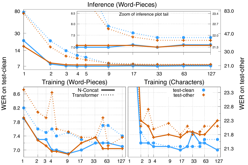
Figure 1: $N$-Concat and Transformer WER on LS100 as a function of the left context length. Both test-clean (blue line) on the left y-axis and test-other (brown dashed line) on the right secondary y-axis are shown in each plot. Legends are shared across all plots. All models use 1 sec EIL chunked encoder.

Table 6: Effect of limiting left context for Transformer (as Transf.) and $N$-Concat PNs on D2P1K dataset measured in WER.

left-context	1	2	3	4	5	6
Transf.	$14.6$	$14.0$	$13.9$	$13.9$	$14.0$	$14.0$
$N$-Concat	$14.4$	$14.0$	$13.9$	$13.9$	$\mathbf{13.8}$	$14.0$

Table 7: WER on test-clean LS100 as we force $2$-Concat online RNN-T to behave like a unigram with a regularization weight.

Reg. weight	0.0	0.01	0.1	1	10	25
$2$-Concat	$7.9$	$8.0$	$7.6$	$7.9$	$9.7$	$24.3$

Table 7 fills the gap between a 1-gram PN (or non-autoregressive), which always diverged in our case, and a bigram word-piece PN by adding a l2 regularization that forces each embedding to be as close as possible to the average learnt embedding. The larger the regularization weight, the more non-autoregressive the model is. As expected, the performance tends to the grade as the regularization weight is increased.

4 Conclusions

We proposed a N-Concat PN that reduces the PN parameters while still outperforming the other PNs in online RNN-T models. We ran extensive experiments with different PNs and found that their performance heavily depends on the acoustic conditions and the encoder regime, either online or batch recognition. In online scenarios the PN becomes more important and an overparametrized PN can hurt performance. For offline recognition, we found that the PN architecture becomes less important than in the online case. Although both Transformer and N-Concat PN are resilient to limited left context at training and inference, N-Concat more efficiently exploits the left context. Both PNs are not able to exploit long-term dependencies and yet limiting the left context to less than 2 tokens severely degrades performance. As future work, we would extend our study to take external language models into account, and exploit the limited n-gram dependency to generate lattices as outputs for downstream tasks.

References

- [1] A. Graves, “Sequence transduction with recurrent neural networks,” in Proc. of ICML Workshop on Representation Learning. Edinburgh, UK: PMLR, 2012.
- [2] A. Graves, S. Fernandez, F. Gomez, and J. Schmidhuber, “Connectionist temporal classification: Labelling unsegmented sequence data with recurrent neural nets,” in ICML ’06: Proceedings of the International Conference on Machine Learning, 2006.
- [3] E. Variani, D. Rybach, C. Allauzen, and M. Riley, “Hybrid autoregressive transducer (hat),” in ICASSP 2020 - 2020 IEEE International Conference on Acoustics, Speech and Signal Processing (ICASSP), 2020, pp. 6139–6143.
- [4] H. Sak, M. Shannon, K. Rao, and F. Beaufays, “Recurrent Neural Aligner: An Encoder-Decoder Neural Network Model for Sequence to Sequence Mapping,” in Proc. Interspeech 2017, 2017, pp. 1298–1302.
- [5] A. Tripathi, H. Lu, H. Sak, and H. Soltau, “Monotonic recurrent neural network transducer and decoding strategies,” in 2019 IEEE Automatic Speech Recognition and Understanding Workshop (ASRU), 2019, pp. 944–948.
- [6] C. feng Yeh, J. Mahadeokar, K. Kalgaonkar, Y. Wang, D. Le, M. Jain, K. Schubert, C. Fuegen, and M. L. Seltzer, “Transformer-transducer: End-to-end speech recognition with self-attention,” ArXiv, vol. abs/1910.12977, 2019.
- [7] Q. Zhang, H. Lu, H. Sak, A. Tripathi, E. McDermott, S. Koo, and S. Kumar, “Transformer Transducer: A streamable speech recognition model with Transformer encoders and RNN-T loss,” in Proc. of ICASSP. Barcelona, Spain: IEEE, 2020, pp. 7829–7833.
- [8] J. Anshuman, Tripathi andKim, Q. Zhang, H. Lu, and H. Sak, “Transformer transducer: One model unifying streaming and non-streaming speech recognition,” 2020.
- [9] A. Gulati, J. Qin, C.-C. Chiu, N. Parmar, Y. Zhang, J. Yu, W. Han, S. Wang, Z. Zhang, Y. Wu et al., “Conformer: Convolution-augmented Transformer for speech recognition,” in Proc. of INTERSPEECH. Shanghai, China: ISCA, 2020, pp. 5036–5040.
- [10] W. Han, Z. Zhang, Y. Zhang, J. Yu, C.-C. Chiu, J. Qin, A. Gulati, R. Pang, and Y. Wu, “ContextNet: Improving convolutional neural networks for automatic speech recognition with global context,” in Proc. Interspeech 2020, 2020, pp. 3610–3614.
- [11] X. Chen, Y. Wu, Z. Wang, S. Liu, and J. Li, “Developing real-time streaming transformer transducer for speech recognition on large-scale dataset,” in ICASSP, June 2021.
- [12] Y. Shi, Y. Wang, C. Wu, C.-F. Yeh, J. Chan, F. Zhang, D. Le, and M. Seltzer, “Emformer: Efficient memory transformer based acoustic model for low latency streaming speech recognition,” in ICASSP 2021 - 2021 IEEE International Conference on Acoustics, Speech and Signal Processing (ICASSP), 2021, pp. 6783–6787.
- [13] Z. Meng, N. Kanda, Y. Gaur, S. Parthasarathy, E. Sun, L. Lu, X. Chen, J. Li, and Y. Gong, “Internal language model training for domain-adaptive end-to-end speech recognition,” in ICASSP, June 2021. [Online]. Available: https://www.microsoft.com/en-us/research/publication/internal-language-model-training-for-domain-adaptive-end-to-end-speech-recognition/
- [14] Z. Meng, Y. Gaur, N. Kanda, J. Li, X. Chen, Y. Wu, and Y. Gong, “Internal language model adaptation with text-only data for end-to-end speech recognition,” arXiv, October 2021.
- [15] E. Weinstein, J. Apfel, M. Ghodsi, R. Cabrera, and X. Liu, “Rnn-transducer with stateless prediction network,” in ICASSP 2020, 2020, pp. 7049–7053.
- [16] Y. Higuchi, N. Chen, Y. Fujita, H. Inaguma, T. Komatsu, J. Lee, J. Nozaki, T. Wang, and S. Watanabe, “A comparative study on non-autoregressive modelings for speech-to-text generation,” in 2021 IEEE Automatic Speech Recognition and Understanding Workshop (ASRU), 2021, pp. 47–54.
- [17] H. Shrivastava, A. Garg, Y. Cao, Y. Zhang, and T. Sainath, “Echo state speech recognition,” in ICASSP 2021 - 2021 IEEE International Conference on Acoustics, Speech and Signal Processing (ICASSP), 2021, pp. 5669–5673.
- [18] R. Botros, T. N. Sainath, R. David, E. Guzman, W. Li, and Y. He, “Tied & Reduced RNN-T Decoder,” in Proc. Interspeech 2021, 2021, pp. 4563–4567.
- [19] Y. Zhang, J. Qin, D. S. Park, W. Han, C. Chiu, R. Pang, Q. V. Le, and Y. Wu, “Pushing the limits of semi-supervised learning for automatic speech recognition,” CoRR, vol. abs/2010.10504, 2020. [Online]. Available: https://arxiv.org/abs/2010.10504
- [20] S. Hochreiter and J. Schmidhuber, “Long short-term memory,” Neural Computation 9, no. 8, pp. 1735–1780, 1997.
- [21] A. Vaswani, N. Shazeer, N. Parmar, J. Uszkoreit, L. Jones, A. N. Gomez, L. u. Kaiser, and I. Polosukhin, “Attention is all you need,” in Advances in Neural Information Processing Systems, I. Guyon, U. V. Luxburg, S. Bengio, H. Wallach, R. Fergus, S. Vishwanathan, and R. Garnett, Eds., vol. 30. Curran Associates, Inc., 2017.
- [22] R. Prabhavalkar, Y. R. He, D. J. Rybach, S. Campbell, A. Narayanan, T. D. Strohman, and T. N. Sainath, “Less is more: Improved rnn-t decoding using limited label context and path merging,” in ICASSP 2021, 2021. [Online]. Available: https://ieeexplore.ieee.org/abstract/document/9414212
- [23] D. S. Park, W. Chan, Y. Zhang, C.-C. Chiu, B. Zoph et al., “SpecAugment: A simple data augmentation method for automatic speech recognition,” in Proc. of INTERSPEECH. Graz, Austria: ISCA, 2019, pp. 2613–2617.
- [24] D. Kingma and J. Ba, “Adam: A method for stochastic optimization,” in ICLR, 2015, 2014. [Online]. Available: http://arxiv.org/abs/1412.6980
- [25] V. Panayotov, G. Chen, D. Povey, and S. Khudanpur, “LibriSpeech: An ASR corpus based on public domain audio books,” in Proc. of ICASSP. Brisbane, Australia: IEEE, 2015, pp. 5206–5210.
- [26] T. Ko, V. Peddinti, D. Povey, and S. Khudanpur, “Audio augmentation for speech recognition,” in Proc. Interspeech 2015, 2015, pp. 3586–3589.