Analysis of Weakly Symmetric Mixed Finite Elements for Elasticity

Abstract.

We consider mixed finite element methods for linear elasticity where the symmetry of the stress tensor is weakly enforced. Both an a priori and a posteriori error analysis are given for several known families of methods that are uniformly valid in the incompressible limit. A posteriori estimates are derived for both the compressible and incompressible cases. The results are verified by numerical examples.

1. Introduction

The purpose of this paper is to give a complete error analysis of mixed finite element methods for linear elasticity where the symmetry of the stress tensor is weakly enforced. In an earlier paper [27] we have analyzed methods with an exact enforcement of symmetry.

The study of mixed methods with the stress tensor and displacement as unknowns goes back to the pioneering work of B. Fraeijs de Veubeke [19]. When the stress tensor is assumed to be exactly symmetric, this leads to methods that are quite complicated and cumbersome to implement. This was also known to Fraeijs de Veubeke, and it lead him to introduce methods for which the symmetry of the stress tensor is enforced in a weak form [20, 17, 18]. The Lagrange multiplier used has the physical meaning of the infinitesimal rotation and the corresponding Euler equation is that of rotational equilibrium.

The mathematical analysis of this class of methods was initiated by Amara and Thomas [1] who considered hybrid methods, and Arnold, Brezzi and Douglas [5] who introduced and analyzed a low-order method. Later, Stenberg [33] introduced a two and three dimensional family. These method all use standard polynomial basis function of Raviart-Thomas and Brezzi-Douglas-Marini type with the addition of divergence free "bubble" degrees of freedom added in order to enforce the stability of the rotational Lagrange multiplier.

The families of the work [33] where reconsidered by Cockburn, Golapakrishnan and Guzmán [15, 22] and they observed that the stabilizing bubble spaces can be reduced. For the two dimensional family this follows by inspecting which degrees of freedom are actually used in the proof given in [33]. In three dimensions, however, their contribution is significant. They introduced a tensor valued bubble function, the use of which reduced the polynomial degree of the divergence free degrees of freedom with one.

In [33] and [22] the polynomials used for the stress and rotation are of the same degree with additional bubbles of one degree higher for the stresses. However, if the degree of the rotation is lowered by one, then the bubbles needed are already contained in the space for the stress. This leads to the family of Arnold, Falk and Winther [7, 9]. It however, leads to a decreased convergence rate for the stress. This lead us to introduce a method in which the normal component of the stress is reduced by one degree on each element edge or face.

In this paper we will perform a unified a priori error analysis covering the methods mentioned above. We essentially use the same analysis as in [33]. In that paper we used the macroelement technique to establish the stability. The idea in this technique is that the crucial requirement for the stability is that the degrees of freedom are such that the local uniqueness (modulo a rigid body motion) is valid. The local stability condition then follows from homogeneity and continuity arguments. Below, we will, however, perform the analysis explicitly.

In addition to the a priori analysis we will perform a novel a posteriori analysis. By modifying the classical Prager-Synge hypercircle theorem [30, 29] we derive an estimate without any unknown constants. This estimate deteriorates for nearly incompressible materials and for that case we introduce another estimate.

The plan of the paper is as follows. In the next section we recall the equations of linear elasticity with the rotational equilibrium as an independent equation. We prove the stability of the problem using the physical energy norms. In the next section we recall the finite element methods and prove the stability and a priori error estimates. In Section 4 we introduce and analyze a post processing of the displacement variable. This is crucial for the a posteriori analysis which is done in Section 5 and Section 6. In the last section we perform numerical benchmark studies.

We use the established notation for Sobolev spaces and finite element methods. We write $A\lesssim B$ when there exists a positive constant $C$, that is independent of the mesh parameter and, in particular, of the two Lamé parameters $\mu,\lambda$ (see below) such that $A\leq CB$. Analogously we define $A\gtrsim B$. $A\lesssim B$ and $A\gtrsim B$ is denoted by $A\simeq B$. We are careful of explicitly including the right physical parameters, and this means that the dependency of the two Lamé parameters are made explicit in the norms used.

2. The equations of elasticity with rotational equilibrium

Let $\Omega\subset{}^{d}$ be a polygonal or polyhedral domain. The physical unknowns are the displacement vector $u=(u_{1},\dots,u_{d})$ and the stress tensor $\sigma=\{\sigma_{ij}\}$, $i,j=1,\dots,d$. The loading consists of a body load $f$ and a traction $g$ on the boundary part $\Gamma_{N}$. On the complementary part $\Gamma_{D}$ homogeneous Dirichlet conditions for the displacement are given.

The condition of force and rotational equilibrium gives the equations

(2.1) $$\mathrm{div}\,\sigma+f=0\ \mbox{ in }\Omega,$$

and

(2.2) $$\sigma-\sigma^{T}=0\ \mbox{ in }\Omega,$$

respectively.

The deformation is given by the infinitesimal strain tensor

(2.3) $$\varepsilon(u)=\frac{1}{2}\big{(}\nabla u+\nabla u^{T}\big{)}.$$

The stress and strain tensors are related by a linear constitutive law. For an isotropic material and the plane strain ($d=2$) or three dimensional ($d=3$) problem this is given by

(2.4) $$\mathcal{C}\sigma=\varepsilon(u),$$

with the compliance tensor

(2.5) $$\mathcal{C}\tau=\frac{1}{2\mu}\Big{(}\tau-\frac{\lambda}{2\mu+d\lambda}{\rm tr}(\tau)I\Big{)},$$

where $\mu\mbox{ and }\lambda$ are the Lamé parameters. For the plane stress problem the relationship is, cf. [29],

(2.6) $$\mathcal{C}\tau=\frac{1}{2\mu}\Big{(}\tau-\frac{\lambda^{*}}{2\mu+2\lambda^{*}}{\rm tr}(\tau)I\Big{)},$$

with

(2.7) $$\lambda^{*}=\frac{2\mu\lambda}{\lambda+2\mu}.$$

The inverse of the compliance matrix, the elasticity matrix, we denote by ${\mathcal{A}}=\mathcal{C}^{-1}$, i.e.

(2.8) $${\mathcal{A}}\tau=2\mu\tau+\lambda{\rm tr}(\tau)I,$$

for the plane strain and three dimensional problem, and

(2.9) $${\mathcal{A}}\tau=2\mu\tau+\lambda^{*}{\rm tr}(\tau)I,$$

for plane stress.

Due to the symmetry of the compliance tensor, the symmetry of the stress tensor is implied by (2.5), (2.6), and the traditional form of the elasticity equations are

(2.10) $$\mathcal{C}\sigma-\varepsilon(u) = 0\ \mbox{ in }\Omega,$$

(2.11) $$\mathrm{div}\,\sigma+f = 0\ \mbox{ in }\Omega,$$

(2.12) $$u = 0\ \mbox{ on }\Gamma_{D},$$

(2.13) $$\sigma n = g\ \mbox{ on }\Gamma_{N}.$$

Using this formulation as a basis for mixed finite element methods leads, however, to rather complicated methods, cf. [25, 6, 4, 23], and this lead Fraeijs de Veubeke to suggest mixed methods in which the rotational equilibrium (2.2) is treated as an independent equation [20, 17]. Due to the introduction of one additional equation, one additional unknown is needed, and this is the skew symmetric infinitesimal rotation, viz.

(2.14) $$\rho=\frac{1}{2}\big{(}\nabla u-\nabla u^{T}\big{)}.$$

This gives the set of equations

(2.15) $$\mathcal{C}\sigma+\rho-\nabla u = 0\ \mbox{ in }\Omega,$$

(2.16) $$\sigma-\sigma^{T} = 0\ \mbox{ in }\Omega,$$

(2.17) $$\mathrm{div}\,\sigma+f = 0\ \mbox{ in }\Omega,$$

(2.18) $$u = 0\ \mbox{ on }\Gamma_{D},$$

(2.19) $$\sigma n = g\ \mbox{ on }\Gamma_{N}.$$

The symmetric part of the first equation (2.15) yields the traditional (2.10), and the skew part gives (2.14).

In the sequel we will use the notation

(2.20) $$\omega(u)=\frac{1}{2}\big{(}\nabla u-\nabla u^{T}\big{)}.$$

The variational form of the problem is: find $\sigma\in[L^{2}(\Omega)]^{d\times d}$, $\rho\in[L^{2}(\Omega)]^{d\times d}_{{\rm skw}}$ and $u\in[H_{D}^{1}(\Omega)]^{d}=\{\,v\in[H^{1}(\Omega)]^{d}\,|\,v|_{\Gamma_{D}}=0\,\}$ such that

(2.21) $${\mathcal{B}}(\sigma,\rho,u;\tau,\eta,v) =(f,v)+\langle g,v\rangle_{\Gamma_{N}}$$

$$\forall(\tau,\eta,v)\in[L^{2}(\Omega)]^{d\times d}\times[L^{2}(\Omega)]^{d\times d}_{{\rm skw}}\times[H_{D}^{1}(\Omega)]^{d},$$

with the bilinear form

(2.22) $${\mathcal{B}}(\sigma,\rho,u;\tau,\eta,v)=(\mathcal{C}\sigma,\tau)+b(\tau;\rho,u)-b(\sigma;\eta,v),$$

where

(2.23) $$b(\tau;\eta,v)=(\tau,\eta)-(\tau,\nabla v).$$

The natural energy norms for analyzing this problem are

(2.24) $$\|\tau\|_{\mathcal{C}}^{2}=(\mathcal{C}\tau,\tau)\ \mbox{ and }\ \|\varepsilon(v)\|_{\mathcal{A}}^{2}=({\mathcal{A}}\varepsilon(v),\varepsilon(v)),$$

which are the double of the strain energy expressed by the stress and displacement, respectively. The Babuška–Brezzi condition is then simply the following identity.

Lemma 1.

It holds that

(2.25) $$\sup_{\tau\in[L^{2}(\Omega)]^{d\times d}}\frac{\big{(}\tau,\varepsilon(v)\big{)}+(\eta-\omega(v),\tau)}{\|\tau\|_{\mathcal{C}}} =\big{(}\|\varepsilon(v)\|_{\mathcal{A}}^{2}+\|\eta-\omega(v)\|_{\mathcal{A}}^{2}\big{)}^{1/2}$$

$$\forall(\eta,v)\in[L^{2}(\Omega)]^{d\times d}_{{\rm skw}}\times[H_{D}^{1}(\Omega)]^{d}.$$

Proof.

For $(\eta,v)\in[L^{2}(\Omega)]^{d\times d}_{{\rm skw}}\times[H_{D}^{1}(\Omega)]^{d}$ given, we choose $\tau\in[L^{2}(\Omega)]^{d\times d}$ by $\tau_{{\rm sym}}={\mathcal{A}}\varepsilon(v)$ and $\tau_{{\rm skw}}={\mathcal{A}}(\eta-\omega(v))$. The claim then follows from the orthogonality between symmetric and skew symmetric tensors. $\Box$

We denote

(2.26) $${E(\Omega)}=[L^{2}(\Omega)]^{d\times d}\times[L^{2}(\Omega)]^{d\times d}_{{\rm skw}}\times[H_{D}^{1}(\Omega)]^{d},$$

and

(2.27) $$\|(\tau,\eta,v)\|_{E(\Omega)}^{2}=\|\tau\|_{\mathcal{C}}^{2}+\|\varepsilon(v)\|_{\mathcal{A}}^{2}+\|\eta-\omega(v)\|_{\mathcal{A}}^{2}.$$

With the use of this energy norm, we first obtain the sharp "inf-sup" estimate above, and by using Lemma 3.1 of [24], we then get the stability with a known constant.

Theorem 1.

It holds that

(2.28) $$\sup_{(\varphi,\xi,z)\in{E(\Omega)}}\frac{{\mathcal{B}}(\tau,\eta,v;\varphi,\xi,z)}{\|(\varphi,\xi,z)\|_{E(\Omega)}} \geq\Big{(}\frac{\sqrt{5}-1}{2}\Big{)}\|(\tau,\eta,v)\|_{E(\Omega)}$$

$$\qquad\qquad\forall(\tau,\eta,v)\in{E(\Omega)}.$$

For nearly incompressible materials the stability has to be posed differently, and we proceed as follows. For $\tau$ we let $\tau^{D}$ be the deviatoric part of $\tau$, defined by the condition ${\rm tr}(\tau^{D})=0.$ Hence, we have

(2.29) $$\tau=\tau^{D}+\frac{1}{d}{\rm tr}(\tau)I.$$

A direct computation gives.

Lemma 2.

For the constitutive law (2.5) it holds that

(2.30) $$(\mathcal{C}\tau,\tau)=\frac{1}{2\mu}\|\tau^{D}\|_{0}^{2}+\frac{1}{2\mu+d\lambda}\|{\rm tr}(\tau)\|_{0}^{2}.$$

From this we see that $\|\cdot\|_{\mathcal{C}}$ ceases to define a norm in the incompressible limit $\lambda\to\infty$. In the general theory of Brezzi [11], the stability follows from the condition of the "ellipticity in the kernel". In [27] we, however, gave an explicit proof. In this part of the stability estimate one has to use the Babuška–Brezzi condition for the Stokes problem [21].

Lemma 3.

It holds that

(2.31) $$\sup_{v\in[H_{D}^{1}(\Omega)]^{d}}\frac{(\mathrm{div}\,v,q)}{\|\varepsilon(v)\|_{0}}\geq\beta\|q\|_{0}\quad\forall q\in L^{2}(\Omega).$$

The Babuška–Brezzi condition we now write as follows.

Lemma 4.

It holds that

(2.32) $$\sup_{\tau\in[L^{2}(\Omega)]^{d\times d}}\frac{\big{(}\tau,\varepsilon(v)\big{)}+(\eta-\omega(v),\tau)}{\mu^{-1/2}\|\tau\|_{0}} =\big{(}\mu\|\varepsilon(v)\|_{0}^{2}+\mu\|\eta-\omega(v)\|_{0}^{2}\big{)}^{1/2}$$

$$\forall(\eta,v)\in[L^{2}(\Omega)]^{d\times d}_{{\rm skw}}\times[H_{D}^{1}(\Omega)]^{d}.$$

The full stability is a consequence of the above results. In the proof, Lemma 2 yields the stability for the deviatoric stress. Inequality (2.31) implies the stability for the hydrostatic pressure part, whereas Lemma 4 yields the control of the displacement and rotation. The proof is similar to that of Theorem 1 of [27] and is omitted. Since the stability constant will dependent on the unknown constant in (2.31), there is no advantage to use an energy-type norm. By Korn’s inequality it holds

$$\|\varepsilon(v)\|_{0}+\|\eta-\omega(v)\|_{0}\simeq\|\varepsilon(v)\|+\|\eta\|_{0},$$

and using this we give the analysis with the norm

(2.33) $$|\!|\!|(\tau,\eta,v)|\!|\!|^{2}=\mu^{-1}\|\tau\|_{0}^{2}+\mu\|\varepsilon(v)\|_{0}^{2}+\mu\|\eta\|_{0}^{2}.$$

Theorem 2.

It holds that

(2.34) $$\sup_{(\varphi,\xi,v)\in{E(\Omega)}}\frac{{\mathcal{B}}(\tau,\eta,v;\varphi,\xi,z)}{|\!|\!|(\varphi,\xi,z)|\!|\!|} \gtrsim|\!|\!|(\tau,\eta,v)|\!|\!|\quad\forall(\tau,\eta,v)\in{E(\Omega)}.$$

The finite element methods are based on a mixed formulation obtained by dualization. The space for the stress is

(2.35) $$H(\mathrm{div}\!:\!\Omega)=\{\,\tau\in[L^{2}(\Omega)]^{d\times d}\,|\,\mathrm{div}\,\tau\in[L^{2}(\Omega)]^{d}\,\},$$

that of the displacement is $[L^{2}(\Omega)]^{d}$ and the rotation is in $[L^{2}(\Omega)]^{d\times d}_{{\rm skw}}$. The bilinear form used is

(2.36) $${\mathcal{M}}(\sigma,\rho,u;\tau,\eta,v)=(\mathcal{C}\sigma,\tau)+b(\tau;\rho,u)+b(\sigma;\eta,v),$$

with

(2.37) $$b(\tau;\rho,u)=(\mathrm{div}\,\tau,u)+(\tau,\rho).$$

The variational formulation is: find $(\sigma,\rho,u)\in H_{g}(\mathrm{div}\,\!\!:\!\Omega)\times[L^{2}(\Omega)]^{d\times d}_{{\rm skw}}\times[L^{2}(\Omega)]^{d}$ such that

(2.38) $${\mathcal{M}}(\sigma,\rho,u ;\tau,\eta,v)+(f,v)=0$$

$$\forall(\tau,\eta,v)\in H_{0}(\mathrm{div}\,\!\!:\!\Omega)\times[L^{2}(\Omega)]^{d\times d}_{{\rm skw}}\times[L^{2}(\Omega)]^{d},$$

with

(2.39) $$H_{g}(\mathrm{div}\,\!\!:\!\Omega)=\{\,\tau\in H({\rm div}\!:\!\Omega)\,|\ \tau n|_{\Gamma_{N}}=g\,\},$$

and

(2.40) $$H_{0}(\mathrm{div}\,\!\!:\!\Omega)=\{\,\tau\in H({\rm div}\!:\!\Omega)\,|\ \tau n|_{\Gamma_{N}}=0\,\}.$$

3. Weakly symmetric mixed finite element methods

The finite element methods are based on the variational formulation (2.38) posed in the subspaces $S_{h}\subset H(\mathrm{div}\!:\!\Omega)$, $R_{h}\subset[L^{2}(\Omega)]^{d\times d}_{{\rm skw}}$ and $V_{h}\subset[L^{2}(\Omega)]^{d}$:

Find $\sigma_{h}\in S_{h}^{g}$, $\rho_{h}\in R_{h}$ and $u_{h}\in V_{h}$ such that

(3.1) $${\mathcal{M}}(\sigma_{h},\rho_{h},u_{h};\tau,\eta,v)+(f,v)=0\quad\forall(\tau,\eta,v)\in S_{h}^{0}\times R_{h}\times V_{h},$$

where

(3.2) $$S_{h}^{g}=\{\tau\in S_{h}\,|\tau n=g_{h}\,\mbox{ on }\Gamma_{N}\},$$

with $g_{h}$ being an approximation of $g$ (see below) and $S_{h}^{0}=S_{h}\cap H_{0}(\mathrm{div}\,\!\!:\!\Omega)$.

We will give an analysis covering the methods mentioned in the introduction, i.e. those of Stenberg [33], Cockburn, Golapakrishnan and Guzmán [15, 22], and Arnold, Falk and Winther [7, 9]. In addition, we will introduce a new method obtained by inspecting the one of Arnold et al.

The finite element partitioning consists of triangles or tetrahedrons and is denoted by ${\mathcal{C}}_{h}$. An edge (for $d=2$) or face ($d=3$) of an element $K\in{\mathcal{C}}_{h}$ we denote by $E$, and the collection of edges/faces is denoted by $\Gamma_{h}$. By $P_{l}(K)$ and $\tilde{P}_{l}(K)$, with $l\geq 0$, we denote the polynomials and homogeneous polynomials of degree $l$, respectively.

For a triangle the scalar valued bubble function $b_{K}$ is defined as

(3.3) $$b_{K}=\lambda_{1}\lambda_{2}\lambda_{3},$$

where $\lambda_{1},\,\lambda_{2},\,\lambda_{3}$ are the barycentric coordinates. For tetrahedrons the tensor valued bubble function is

(3.4) $$b_{K}=\sum_{l=0}^{3}\lambda_{l-3}\lambda_{l-2}\lambda_{l-1}\nabla\lambda_{l}^{T}\nabla\lambda_{l},$$

where the sum is calculated modulo four, and $\nabla\lambda_{l}$ is considered as a row vector. In both dimensions it holds that the bubble is a third degree polynomial. The bubble induces a weighted inner product on $K\in{\mathcal{C}}_{h}$, viz.

(3.5) $$(wb_{K},v)_{K}=(vb_{K},w)_{K},\ (vb_{K},v)_{K}\geq 0,\mbox{ and }(vb_{K},v)_{K}=0\ \Rightarrow v=0.$$

With the aid of the bubble we define

(3.6) $$M_{l+1}(K)=\{\,\tau\,|\,\tau={\rm curl}\,\big{(}{\rm curl}\,(z)b_{K}),\,z\in[P_{l}(K)]^{d\times d}_{{\rm skw}}\,\},$$

for $l=k-1$ and $l=k$. Here the ${\rm curl}\,$ is applied row wise to the tensors. The functions in this space have both vanishing normal components at the boundary and a vanishing divergence, viz.

(3.7) $$\tau n|_{\partial K}=0,\quad\mathrm{div}\,\tau=0,\quad\forall\tau\in M_{l+1}(K).$$

We furter note that by the definition of the bubble function $b_{K}$ the index of the space $M_{l+1}(K)$ refers to the polynomial order $l+1$ of the corresponding functions for both $d=2$ and $d=3$. The Raviart-Thomas space on $K$ is

(3.8) $$RT_{k-1}(K)=[P_{k-1}(K)]^{d}\oplus x\tilde{P}_{k-1}(K).$$

The tensors with the rows in $RT_{k-1}(K)$ is denoted by

(3.9) $$[RT_{k-1}(K)]^{d}.$$

Next we define the methods to be analyzed.

• The finite element space for the displacement is the same for all families, and we index it with $k\geq 1$:

  (3.10) $$V_{h}=\{\,v\in[L^{2}(\Omega)]^{d}\,|\ v|_{K}\in[P_{k-1}(K)]^{d}\ \forall K\in{\mathcal{C}}_{h}\}.$$

• In the Cockburn-Golapakrishnan-Guzmán family (CGG) [15] the space for the rotation is defined by piecewise polynomials of degree $k-1\geq 1$

  (3.11) $$R_{h}=\{\,\eta\in[L^{2}(\Omega)]^{d\times d}_{{\rm skw}}\ |\ \eta|_{K}\in[P_{k-1}(K)]^{d\times d}_{{\rm skw}}\ \forall K\in{\mathcal{C}}_{h}\},$$

  and that of the stress uses the Raviart-Thomas spaces and the bubble space defined above

  (3.12) $$S_{h}=\{\,\tau\in H(\mathrm{div}\!:\!\Omega)\,|\,\tau|_{K}\in[RT_{k-1}(K)]^{d}+M_{k}(K)\ \forall K\in{\mathcal{C}}_{h}\}.$$

  In the error analysis below we will show that for a smooth solution this method yields the convergence rate

  (3.13) $$\|\sigma-\sigma_{h}\|_{0}\lesssim h^{k},$$

  which is optimal, i.e. the same as the interpolation with this approximation space for the stress.

• The Golapakrishnan and Guzmán [22] refinement of Stenbergs method [33] consists of the above choice of $V_{h}$, and

  (3.14) $$R_{h}=\{\,\eta\in[L^{2}(\Omega)]^{d\times d}_{{\rm skw}}\ |\ \eta|_{K}\in[P_{k}(K)]^{d\times d}_{{\rm skw}}\ \forall K\in{\mathcal{C}}_{h}\},$$

  and

  (3.15) $$S_{h}=\{\,\tau\in H(\mathrm{div}\!:\!\Omega)\,|\,\tau|_{K}\in[P_{k}(K)]^{d\times d}+M_{k+1}(K)\ \forall K\in{\mathcal{C}}_{h}\},$$

  with $k\geq 1.$ Below the family is referred to as SGG. The convergence rate is now also optimal

  (3.16) $$\|\sigma-\sigma_{h}\|_{0}\lesssim h^{k+1}.$$

• In the Arnold-Falk-Winther family (AFW) [7, 9] the polynomial degree for the rotation is lowered by one, and a consequence of that, is that the additional bubble degrees of freedom are not needed. The spaces are then defined for $k\geq 1$ by

  (3.17) $$S_{h}=\{\,\tau\in H(\mathrm{div}\!:\!\Omega)\,|\,\tau|_{K}\in[P_{k}(K)]^{d\times d}\ \forall K\in{\mathcal{C}}_{h}\},$$

  and

  (3.18) $$R_{h}=\{\,\eta\in[L^{2}(\Omega)]^{d\times d}_{{\rm skw}}\ |\ \eta|_{K}\in[P_{k-1}(K)]^{d\times d}_{{\rm skw}}\ \forall K\in{\mathcal{C}}_{h}\}.$$

  The drawback of this choice is that the polynomials chosen for the unknowns are not in balance, and as a consequence the convergence rate is not optimal. It holds

  (3.19) $$\|\sigma-\sigma_{h}\|_{0}\lesssim h^{k},$$

  which should be compared with

  (3.20) $$\inf_{\tau\in S_{h}}\|\sigma-\tau\|_{0}\lesssim h^{k+1}.$$

• This motivates the following modification which appears to be new. On each inter element boundary the polynomial order is reduced by one. We set

  (3.21) $$S_{k}^{r}(K)=\{\,v\in[P_{k}(K)]^{d\times d}\,|\ vn|_{E}\in[P_{k-1}(E)]^{d}\ \forall E\subset\partial K\}$$

  and define the stress space for $k\geq 2$ as

  (3.22) $$S_{h}=\{\,\tau\in H(\mathrm{div}\!:\!\Omega)\,|\,\tau|_{K}\in S_{k}^{r}(K)\ \forall K\in{\mathcal{C}}_{h}\}.$$

  The space for the rotation is as in the original method. This method we will refer to as RAFW (reduced AFW).

  As the most efficient method of solving the finite element system is by hybridization [3], the decrease of the normal degrees of freedom on element boundaries leads to a decrease of computational cost compared with the corresponding AFW method, but with the same accuracy, i.e., (3.19). Most drastically this is seen for the lowest order method, with $k=2$, for which the numbers of unknowns are halved.

In the methods $g_{h}|_{E}=Q_{E}g\,$ with the $L^{2}$ projection $Q_{E}:[L^{2}(E)]^{d}\to[P_{l}(E)]^{d}$, with $l=k$ for SGG and AFW, and $l=k-1$ for the others. Further, we define $Q_{h}$ by $Q_{h}|_{E}=Q_{E}$.

In the error analysis we will use the broken energy norm for the displacement

(3.23) $$\|v\|_{h}=\big{(}\sum_{K\in{\mathcal{C}}_{h}}\|\varepsilon(v)\|_{0,K}^{2}+\sum_{E\in\Gamma_{h}}h_{E}^{-1}\|[\![v]\!]\|_{0,E}^{2}+\sum_{E\subset\Gamma_{D}}h_{E}^{-1}\|v\|_{0,E}^{2}\big{)}^{1/2}.$$

In the proof of the discrete Babuška–Brezzi stability condition we first obtain the stability in the norm

(3.24) $$\|v\|_{h}^{2}+\sum_{K\in{\mathcal{C}}_{h}}\|\eta-\omega(v)\|_{0,K}^{2}\quad\forall(v,\eta)\in V_{h}\times R_{h}.$$

From the discrete Korn inequality [12] it follows that

(3.25) $$\|v\|_{h}^{2}\gtrsim\sum_{K\in{\mathcal{C}}_{h}}\|\omega(v)\|_{0,K}^{2}\quad\forall v\in V_{h},$$

This implies the norm equivalence.

Lemma 5.

It holds that

(3.26) $$\|v\|_{h}^{2}+\sum_{K\in{\mathcal{C}}_{h}}\|\eta-\omega(v)\|_{0,K}^{2}\simeq\|v\|_{h}^{2}+\|\eta\|_{0}^{2}\quad\forall(v,\eta)\in V_{h}\times R_{h}.$$

Hence, we will use the norm

(3.27) $$|\!|\!|(\tau,\eta,v)|\!|\!|_{h}^{2}=\mu^{-1}\|\tau\|_{0}^{2}+\mu\|v\|_{h}^{2}+\mu\|\eta\|_{0}^{2}.$$

The discrete Babuška-Brezzi is the following.

Lemma 6.

Let $b$ be the bilinear form (2.37). It holds that

(3.28) $$\sup_{\tau\in S_{h}^{0}}\frac{b(\tau;\eta,v)}{\|\tau\|_{0}}\gtrsim(\|\eta\|_{0}+\|v\|_{h})\quad\forall(v,\eta)\in V_{h}\times R_{h}.$$

In the proof we proceed differently for the cases $k\geq 2$ and $k=1$. For the first case we need an additional result. Define

(3.29) $$R_{h}^{0}=\{\,\eta\in R_{h}\,|\,\eta|_{K}\in[P_{0}(K)]^{d\times d}_{{\rm skw}}\ \forall K\in{\mathcal{C}}_{h}\,\},$$

and let $N_{h}:R_{h}\to R_{h}^{0}$ be the $L^{2}$ projection.

Lemma 7.

It holds that

(3.30) $$\sup_{\tau\in M_{l+1}(K)}\frac{(\tau,\eta)_{K}}{\|\tau\|_{0,K}}\gtrsim\|\eta-N_{h}\eta\|_{0,K}\quad\forall\eta\in[P_{l}(K)]^{d\times d}_{{\rm skw}}.$$

Proof.

For $\eta\in[P_{l}(K)]^{d\times d}_{{\rm skw}}$ given, we choose $\tau\in M_{l+1}(K)$ by

(3.31) $$\tau|_{K}=h_{K}^{2}{\rm curl}\,\big{(}{\rm curl}\,(\eta)b_{K}\big{)}.$$

Integration by parts gives

(3.32) $$(\tau,\eta)_{K}=h_{K}^{2}({\rm curl}\,(\eta)b_{K},{\rm curl}\,\eta)_{K}\gtrsim h_{K}^{2}\|{\rm curl}\,\eta\|_{0,K}^{2}.$$

Since, $\eta$ is skew symmetric it holds

(3.33) $$\|\eta-N_{h}\eta\|_{0,K}\lesssim h_{K}\|\nabla\eta\|_{0,K}\lesssim h_{K}\|{\rm curl}\,\eta\|_{0,K}.$$

By the inverse inequality we have

(3.34) $$\|\tau\|_{0,K}^{2} =h_{K}^{2}\|{\rm curl}\,\big{(}{\rm curl}\,(\eta)b_{K}\big{)}\|_{0,K}^{2}=h_{K}^{2}\|{\rm curl}\,\big{(}{\rm curl}\,(\eta-N_{h}\eta)b_{K}\big{)}\|_{0,K}^{2}$$

$$\lesssim\|\eta-N_{h}\eta\|_{0,K}^{2}.$$

$\Box$

Using this result we give the

Proof of Lemma 6 for $k\geq 2$. We first note that $V_{h}$ is the same for all methods considered. We define

(3.35) $$\widetilde{RT}_{k-1}(K)=\{\,\tau\in RT_{k-1}(K)\,|\,\,\tau\cdot n|_{E}\in P_{1}(E)\ \forall E\subset\partial K\,\}.$$

The degrees of freedom of this space are [11]

(3.36) $$\int_{K}\tau\cdot v,\ v\in[P_{k-2}(K)]^{d}\ \mbox{ and }\int_{E}(\tau\cdot n)v,\ v\in P_{1}(E),\ E\subset\partial K.$$

By $Q_{E}^{1}:[L^{2}(E)]^{d}:\to[P_{1}(E)]^{d}$ we denote the $L^{2}$ projection.

Let $(v,\eta)\in V_{h}\times R_{h}$ be given. For $\tau_{1}\in S_{h}$, with $\tau_{1}|_{K}\in[\widetilde{RT}_{k-1}(K)]^{d}\subset S_{h}|_{K}$, it holds

(3.37) $$b(\tau_{1}; v,\eta)=(\mathrm{div}\,\tau_{1},v)+(\tau_{1},\eta)$$

$$= -\sum_{K\in{\mathcal{C}}_{h}}(\tau_{1},\nabla v)_{K}+\sum_{E\in\Gamma_{h}}\int_{E}(\tau_{1}n)\!\cdot\![\![v]\!]+\sum_{E\subset\Gamma_{D}}\int_{E}(\tau_{1}n)\!\cdot\!v+(\tau_{1},\eta)$$

$$= -\sum_{K\in{\mathcal{C}}_{h}}(\tau_{1},\nabla v)_{K}+\sum_{E\in\Gamma_{h}}\int_{E}(\tau_{1}n)\!\cdot\![\![Q_{E}^{1}v]\!]+\sum_{E\subset\Gamma_{D}}\int_{E}(\tau_{1}n)\!\cdot\!Q_{E}^{1}v+(\tau_{1},\eta)$$

$$= \sum_{K\in{\mathcal{C}}_{h}}(\tau_{1},N_{h}\eta-\nabla v)_{K}+\sum_{E\in\Gamma_{h}}\int_{E}(\tau_{1}n)\!\cdot\![\![Q_{E}^{1}v]\!]+\sum_{E\subset\Gamma_{D}}\int_{E}(\tau_{1}n)\!\cdot\!Q_{E}^{1}v$$

$$+(\tau_{1},\eta-N_{h}\eta).$$

By (3.36) we can now choose $\tau_{1}$ such that

(3.38) $$\sum_{K\in{\mathcal{C}}_{h}}(\tau_{1},N_{h}\eta-\nabla v)_{K}+\sum_{E\in\Gamma_{h}}\int_{E}(\tau_{1}n)\!\cdot\![\![v]\!]+\sum_{E\subset\Gamma_{D}}\int_{E}(\tau_{1}n)\!\cdot\!v$$

$$= \sum_{K\in{\mathcal{C}}_{h}}\|N_{h}\eta-\nabla v\|_{0,K}^{2}+\sum_{E\in\Gamma_{h}}h_{E}^{-1}\int_{E}|[\![Q^{1}_{E}v]\!]|^{2}+\sum_{E\subset\Gamma_{D}}h_{E}^{-1}\int_{E}|Q^{1}_{E}v|^{2},$$

and

(3.39) $$\|\tau_{1}\|_{0}\leq C_{1}\Big{(}\sum_{K\in{\mathcal{C}}_{h}}\|N_{h}\eta-\nabla v\|_{0,K}^{2}+\sum_{E\in\Gamma_{h}}h_{E}^{-1}\int_{E}|[\![Q^{1}_{E}v]\!]|^{2}+\sum_{E\subset\Gamma_{N}}h_{E}^{-1}\int_{E}|Q^{1}_{E}v|^{2}\Big{)}^{1/2}.$$

Note that $M_{l+1}(K)\subset S_{h}|_{K}$, with $l=k-1$ for CGG, AFW, RAFW, and $l=k$ for SGG. Using Lemma 7 we then choose $\tau_{2}|_{K}\in M_{l+1}(K)$, such that $\mathrm{div}\,\tau_{2}=0$,

(3.40) $$(\tau_{2},\eta)=\|\eta-N_{h}\eta\|_{0}^{2},\quad\mbox{ and }\quad\|\tau_{2}\|_{0}\leq C_{2}\|\eta-N_{h}\eta\|_{0}.$$

For $\tau=\delta\tau_{1}+\tau_{2}$, with $\delta>0$, it then holds

(3.41) $$b(\tau;v,\eta)= (\mathrm{div}\,\tau,v)+(\tau,\eta)=(\mathrm{div}\,\delta\tau_{1},v)+(\delta\tau_{1}+\tau_{2},\eta)$$

$$= \delta\Big{(}-\sum_{K\in{\mathcal{C}}_{h}}(\tau_{1},\nabla v)_{K}+\sum_{E\in\Gamma_{h}}\int_{E}(\tau_{1}n)\!\cdot\![\![v]\!]+\sum_{E\subset\Gamma_{D}}\int_{E}(\tau_{1}n)\!\cdot\!v\Big{)}$$

$$+(\delta\tau_{1}+\tau_{2},\eta)$$

$$= \delta\Big{(}\sum_{K\in{\mathcal{C}}_{h}}(\tau_{1},N_{h}\eta-\nabla v)_{K}+\sum_{E\in\Gamma_{h}}\int_{E}(\tau_{1}n)\!\cdot\![\![v]\!]+\sum_{E\subset\Gamma_{D}}\int_{E}(\tau_{1}n)\!\cdot\!v\Big{)}$$

$$+\delta(\tau_{1},\eta-N_{h}\eta)+(\tau_{2},\eta).$$

By Schwarz and the arithmetic geometric mean inequality we have

(3.42) $$\delta(\tau_{1},\eta-N_{h}\eta)\geq-\delta\|\tau_{1}\|_{0}\|\eta-N_{h}\eta\|_{0}\geq-\frac{\delta^{2}}{2}\|\tau_{1}\|_{0}^{2}-\frac{1}{2}\|\eta-N_{h}\eta\|_{0}^{2}.$$

Hence, using (3.38), (3.39), and (3.40), it holds

(3.43) $$b(\tau;v,\eta)\geq$$

$$\delta\big{(}1-\frac{\delta C_{1}}{2}\big{)}\Big{(}\sum_{K\in{\mathcal{C}}_{h}}\|N_{h}\eta-\nabla v\|_{0,K}^{2}+\sum_{E\in\Gamma_{h}}h_{E}^{-1}\int_{E}|[\![Q^{1}_{E}v]\!]|^{2}+\sum_{E\subset\Gamma_{D}}h_{E}^{-1}\int_{E}|Q^{1}_{E}v|^{2}\Big{)}$$

$$+\frac{1}{2}\|\eta-N_{h}\eta\|_{0}^{2}.$$

When choosing $0<\delta<2C_{1}^{-1}$, we have

(3.44) $$b(\tau;v,\eta)\gtrsim\sum_{K\in{\mathcal{C}}_{h}} \|N_{h}\eta-\nabla v\|_{0,K}^{2}+\sum_{E\in\Gamma_{h}}h_{E}^{-1}\int_{E}|[\![Q^{1}_{E}v]\!]|^{2}$$

$$+\sum_{E\subset\Gamma_{D}}h_{E}^{-1}\int_{E}|Q^{1}_{E}v|^{2}\ +\|\eta-N_{h}\eta\|_{0}^{2},$$

and

(3.45) $$\|\tau\|_{0}\lesssim\Big{(}\sum_{K\in{\mathcal{C}}_{h}} \|N_{h}\eta-\nabla v\|_{0,K}^{2}+\sum_{E\in\Gamma_{h}}h_{E}^{-1}\int_{E}|[\![Q^{1}_{E}v]\!]|^{2}$$

$$+\sum_{E\subset\Gamma_{D}}h_{E}^{-1}\int_{E}|Q^{1}_{E}v|^{2}+\|\eta-N_{h}\eta\|_{0}^{2}\Big{)}^{1/2}.$$

By the orthogonality between symmetric and skew symmetric tensors we get

(3.46) $$\|N_{h}\eta-\nabla v\|_{0,K}^{2}=\|N_{h}\eta-\omega(v)\|_{0,K}^{2}+\|\varepsilon(v)\|_{0,K}^{2}.$$

The triangle inequality yields

(3.47) $$\|\eta-N_{h}\eta\|_{0,K}^{2}+\|N_{h}\eta-\omega(v)\|_{0,K}^{2}+\|\varepsilon(v)\|_{0,K}^{2}$$

$$\gtrsim\|\eta-\omega(v)\|_{0,K}^{2}+\|\varepsilon(v)\|_{0,K}^{2},$$

and by scaling we have

(3.48) $$\sum_{K\in{\mathcal{C}}_{h}}\|\varepsilon(v)\|_{0,K}^{2}+\sum_{E\in\Gamma_{h}}h_{E}^{-1}\int_{E}|[\![Q^{1}_{E}v]\!]|^{2}+\sum_{E\subset\Gamma_{D}}h_{E}^{-1}\int_{E}|Q^{1}_{E}v|^{2}$$

$$\simeq\sum_{K\in{\mathcal{C}}_{h}}\|\varepsilon(v)\|_{0,K}^{2}+\sum_{E\in\Gamma_{h}}h_{E}^{-1}\int_{E}|[\![v]\!]|^{2}+\sum_{E\subset\Gamma_{D}}h_{E}^{-1}\int_{E}|v|^{2}.$$

Combining the above estimates proves that

(3.49) $$\sup_{\tau\in S_{h}^{0}}\frac{b(\tau;\eta,v)}{\|\tau\|_{0}}\gtrsim\big{(}\ \|v\|_{h}^{2}+\sum_{K\in{\mathcal{C}}_{h}}\|\eta-\omega(v)\|_{0,K}^{2}\big{)}^{17/2}\quad\forall(v,\eta)\in V_{h}\times R_{h},$$

and the assertion follows from the norm equivalence of Lemma 5.

$\square$

Next, we consider the low order methods, the families SGG and AFW with $k=1$, i.e. methods with piecewise constants for the displacement. The rigid body motions on $K$ we denote by

(3.50) $$RM(K)=\begin{cases}\{\,v\,|\,v=(a,b)+c(-x_{2},x_{1}),\ a,b,c\in\real\,\}&\mbox{ for }d=2,\\ \{\,v\,|\,v=a+b\times x,\,a,b\in{}^{3}\,\}&\mbox{ for }d=3.\end{cases}$$

With this we define

(3.51) $$RM_{h}=\{\,\psi\,|\,\psi|_{K}\in RM(K)\ \forall K\in{\mathcal{C}}_{h}\,\}.$$

For $N_{h}\eta\in R_{h}^{0}$ (note that $\eta$ is linear for SGG with $k=1$) there exist a unique $r(N_{h}\eta)\in RM_{h}$ such that

(3.52) $$N_{h}\eta|_{K} =\omega\big{(}r(N_{h}\eta|_{K})\big{)}=\nabla r(N_{h}\eta|_{K}),$$

(3.53) and $$\int_{K}r(N_{h}\eta)=0\quad\forall K\in{\mathcal{C}}_{h}.$$

Let us now give the

Proof of Lemma 6 for the families SGG and AFW, with $k=1$.

Consider first AFW with

(3.54) $$S_{h}=\{\,\tau\in H(\mathrm{div}\!:\!\Omega)\,|\,\tau|_{K}\in[P_{1}(K)]^{d\times d}\ K\in{\mathcal{C}}_{h}\,\},$$

and

(3.55) $$R_{h}=\{\,\eta\in[L^{2}(\Omega)]^{d\times d}_{{\rm skw}}\ |\ \eta|_{K}\in[P_{0}(K)]^{d\times d}_{{\rm skw}}\ \forall K\in{\mathcal{C}}_{h}\,\}.$$

Let $(v,\eta)\in V_{h}\times R_{h}$ be given. Now, $R_{h}^{0}=R_{h}$ and we write $\eta|_{K}=\nabla(r(\eta|_{K}))$. Since $\mathrm{div}\,\tau|_{K}\in P_{0}(K)$, (3.53) gives

(3.56) $$(\tau,\eta) =\sum_{K\in{\mathcal{C}}_{h}}\big{(}\tau,\nabla r(\eta)\big{)}_{K}$$

$$=-\sum_{K\in{\mathcal{C}}_{h}}\big{(}\mathrm{div}\,\tau,r(\eta)\big{)}_{K}+\sum_{E\in\Gamma_{h}}\int_{E}(\tau n)\!\cdot\![\![r(\eta)]\!]+\sum_{E\subset\Gamma_{D}}\int_{E}(\tau n)\!\cdot\!r(\eta)$$

$$=\sum_{E\in\Gamma_{h}}\int_{E}(\tau n)\!\cdot\![\![r(\eta)]\!]+\sum_{E\subset\Gamma_{D}}\int_{E}(\tau n)\!\cdot\!r(\eta).$$

On the other hand, for $(\mathrm{div}\,\tau,v)$ we have

(3.57) $$(\mathrm{div}\,\tau,v) =\sum_{K\in{\mathcal{C}}_{h}}(\mathrm{div}\,\tau,v)_{K}$$

$$=-\sum_{K\in{\mathcal{C}}_{h}}(\tau,\nabla v)_{K}+\sum_{E\in\Gamma_{h}}\int_{E}(\tau n)\!\cdot\![\![v]\!]+\sum_{E\subset\Gamma_{D}}\int_{E}(\tau n)\!\cdot\!v$$

$$=\sum_{E\in\Gamma_{h}}\int_{E}(\tau n)\!\cdot\![\![v]\!]+\sum_{E\subset\Gamma_{D}}\int_{E}(\tau n)\!\cdot\!v.$$

Hence,

(3.58) $$b(\tau;\eta,v) =(\mathrm{div}\,\tau,v)+(\tau,\eta)$$

$$=\sum_{E\in\Gamma_{h}}\int_{E}(\tau n)\!\cdot\!\big{(}[\![r(\eta)+v]\!]\big{)}+\sum_{E\subset\Gamma_{D}}\int_{E}(\tau n)\!\cdot\!\big{(}r(\eta)+v\big{)}.$$

We now choose $\tau$ such that

(3.59) $$\tau n=h_{E}^{-1}\big{(}[\![r(\eta)+v]\!])\ \mbox{ on }E\subset\Gamma_{h},\ \mbox{ and }\tau n=h_{E}^{-1}\big{(}r(\eta)+v)\ \mbox{ on }E\subset\Gamma_{D},$$

which gives

(3.60) $$b(\tau;\eta,v)=\sum_{E\in\Gamma_{h}}h_{E}^{-1}\int_{E}\big{(}[\![r(\eta)+v]\!]\big{)}^{2}+\sum_{E\subset\Gamma_{D}}h_{E}^{-1}\int_{E}\big{(}r(\eta)+v\big{)}^{2},$$

and by scaling

(3.61) $$\|\tau\|_{0}\lesssim\Big{(}\sum_{E\in\Gamma_{h}}h_{E}^{-1}\int_{E}\big{(}[\![r(\eta)+v]\!]\big{)}^{2}+\sum_{E\subset\Gamma_{D}}h_{E}^{-1}\int_{E}\big{(}r(\eta)+v\big{)}^{2}\Big{)}^{1/2}.$$

Since $\varepsilon(r(\eta)+v)|_{K}=0$, the discrete Korn inequality (5.7) gives

(3.62) $$\|r(\eta)+v\|_{h}\lesssim\Big{(}\sum_{E\in\Gamma_{h}}h_{E}^{-1}\int_{E}\big{(}[\![r(\eta)+v]\!]\big{)}^{2}+\sum_{E\subset\Gamma_{D}}h_{E}^{-1}\int_{E}\big{(}r(\eta)+v\big{)}^{2}\Big{)}^{1/2}.$$

Next, (3.52) gives

(3.63) $$\| r(\eta)+v\|_{h}^{2}=\|\eta\|_{0}^{2}$$

$$+\Big{(}\sum_{E\in\Gamma_{h}}h_{E}^{-1}\int_{E}\big{(}[\![r(\eta)+v]\!]\big{)}^{2}+\sum_{E\subset\Gamma_{D}}h_{E}^{-1}\int_{E}\big{(}r(\eta)+v\big{)}^{2}\Big{)}.$$

By scaling arguments we get

(3.64) $$\|\eta\|_{0}^{2} +\Big{(}\sum_{E\in\Gamma_{h}}h_{E}^{-1}\int_{E}\big{(}[\![r(\eta)+v]\!]\big{)}^{2}+\sum_{E\subset\Gamma_{D}}h_{E}^{-1}\int_{E}\big{(}r(\eta)+v\big{)}^{2}\Big{)}$$

$$\simeq\|\eta\|_{0}^{2}+\|v\|_{h}^{2},$$

and the assertion is established for AFW.

For the lowest order SGG the finite element space for the deflection is the same, and that of the rotation is of one degree higher. In this case $\eta\in R_{h}$ is split as $\eta=N_{h}\eta+(I-N_{h})\eta$. The stability of the part $\|N_{h}\eta\|_{0}+\|v\|_{h}$ is established as above, and for the part $\|(I-N_{h})\eta\|_{0}$ the degrees of freedoms in $M_{2}(K)$ are used, following the same arguments as in the proof of Lemma 6 for $k>1$. $\square$

In addition to the stability estimate (3.28), the following property is needed in order to get an optimal a priori error estimate

(3.65) $$\mathrm{div}\,\tau\in V_{h}\quad\forall\tau\in S_{h}.$$

From this it follows that

(3.66) $$(\mathrm{div}\,\tau,v-P_{h}v)=0\quad\forall\tau\in S_{h},$$

where $P_{h}:[L^{2}(\Omega)]^{d}\to V_{h}$ is the $L^{2}$ projection.

To obtain a stability estimate uniformly valid with respect to the incompressibility we will use the following estimate.

Lemma 8.

It holds that

(3.67) $$\sup_{v\in V_{h}}\frac{(v,\mathrm{div}\,\tau)}{\|v\|_{h}}\geq C_{1}\|{\rm tr}(\tau)\|_{0}-C_{2}\|\tau^{D}\|_{0}\quad\forall\tau\in S_{h}^{0}.$$

Proof.

Given $\tau\in S_{h}^{0}$, (2.31) implies that there exists $z\in[H_{D}^{1}(\Omega)]^{d}$ such that

(3.68) $$(\mathrm{div}\,v,{\rm tr}(\tau))=-\beta\|{\rm tr}(\tau)\|_{0}^{2}\ \mbox{and }\ \|\varepsilon(v)\|_{0}=\|{\rm tr}(\tau)\|_{0}.$$

Let $P_{h}v\in V_{h}$ be the projection in (3.66). It holds

(3.69) $$(P_{h}v ,\mathrm{div}\,\tau)=(v,\mathrm{div}\,\tau)=-(\varepsilon(v),\tau)$$

$$=-(\mathrm{div}\,v,{\rm tr}(\tau))-(\varepsilon(v),\tau^{d})\geq\beta\|{\rm tr}(\tau)\|_{0}^{2}-\|\varepsilon(v)\|\|\tau^{d}\|_{0}$$

$$=\|\varepsilon(v)\|_{0}\|_{0}\big{(}\beta\|{\rm tr}(\tau)\|_{0}-\|\tau^{d}\|_{0}\big{)}.$$

By scaling we have

(3.70) $$\|P_{h}v\|_{h}\lesssim\|\varepsilon(v)\|_{0}.$$

Combining the two estimates above proves the claim. $\Box$

From Lemma 2, Lemma 6, and Lemma 8, we get the stability of the method.

Theorem 3.

It holds that

(3.71) $$\sup_{(\varphi,\xi,v)\in S_{h}^{0}\times R_{h}\times V_{h}}\frac{{\mathcal{M}}(\tau,\eta,v;\varphi,\xi,z)}{|\!|\!|(\varphi,\xi,z)|\!|\!|_{h}} \gtrsim|\!|\!|(\tau,\eta,v)|\!|\!|_{h}$$

$$\qquad\forall(\tau,\eta,v)\in S_{h}^{0}\times R_{h}\times V_{h}.$$

In the proof of the error estimate we will use an averaging interpolation operator applied to the discrete displacement space. For $k\geq 2$ it is defined as the so called Oswald interpolation $I_{h}^{a}:V_{h}\to V_{h}\cap[H^{1}_{D}(\Omega)]^{d}$ (cf. [16, Chapter 5.5.2]), which satisfies

(3.72) $$\|\nabla I_{h}^{a}v\|_{0}\ +\Big{(}\sum_{K\in{\mathcal{C}}_{h}}h_{K}^{-2}\|v-I_{h}^{a}v\|_{0,K}^{2}\Big{)}^{1/2}\lesssim\|v\|_{h}.$$

For $k=1$ the displacement space is

(3.73) $$V_{h}^{0}=\{\,v\in[L^{2}(\Omega)]^{d}\,|\ v|_{K}\in[P_{0}(K)]^{d}\ \forall K\in{\mathcal{C}}_{h}\},$$

and for this we define the operator $I_{h}^{a}:V_{h}^{0}:\to V_{h}^{1}\cap[H_{D}(\Omega)]^{d}$, with

(3.74) $$V_{h}^{1}=\{\,v\in[L^{2}(\Omega)]^{d}\,|\ v|_{K}\in[P_{1}(K)]^{d}\ \forall K\in{\mathcal{C}}_{h}\},$$

in the following way. The vertex values of $I_{h}^{a}v$ are the average of the values of $v$ in the elements sharing that vertex, and letting $I_{h}^{a}v=0$ on $\Gamma_{D}$. It is easily proved that this interpolation satisfies (3.72).

We will next derive the quasi-optimality of the methods. Here $f_{h}$ is any piecewise polynomial approximation of $f$.

Theorem 4.

It holds that

(3.75) $$\mu^{-1/2}\| \sigma-\sigma_{h}\|_{0}+\mu^{1/2}(\|P_{h}u-u_{h}\|_{h}+\|\rho-\rho_{h}\|_{0})$$

$$\lesssim\,\mu^{-1/2} \big{(}\inf_{\tau\in S_{h}^{g}}\|\sigma-\tau\|_{0}+\big{(}\sum_{K\in{\mathcal{C}}_{h}}h_{K}^{2}\|f-f_{h}\|_{0,K}^{2}\big{)}^{1/2}\big{)}$$

$$+\inf_{\eta\in R_{h}}\mu^{1/2}\|\rho-\eta\|_{0}.$$

Proof.

By Theorem 3 there exist $(\varphi,\xi,v)\in S_{h}^{0}\times R_{h}\times V_{h}$ with

(3.76) $$|\!|\!|(\varphi,\xi,v)|\!|\!|_{h}=1,$$

such that for all $\tau\in S_{h}^{g}$ and $\eta\in R_{h}$ we have

(3.77) $$\mu^{-1/2}\|\sigma_{h}-\tau\|_{0} +\mu^{1/2}(\|\rho_{h}-\eta\|_{0}+\|P_{h}u-u_{h}\|_{h})$$

$$\lesssim{\mathcal{M}}(\sigma_{h}-\tau,\rho_{h}-\eta,u_{h}-P_{h}u;\varphi,\xi,v).$$

By the consistency we have

(3.78) $${\mathcal{M}}(\sigma_{h}-\tau,\rho_{h}-\eta,u_{h}-P_{h}u;\varphi,\xi,v)={\mathcal{M}}(\sigma-\tau,\rho-\eta,u-P_{h}u;\varphi,\xi,v).$$

Writing out gives

(3.79) $${\mathcal{M}}(\sigma-\tau, \rho-\eta,u-P_{h}u;\varphi,\xi,v)$$

$$= (\mathcal{C}(\sigma-\tau),\varphi)+(\rho-\eta,\varphi)+(u-P_{h}u,\mathrm{div}\,\varphi)$$

$$+(\sigma-\tau,\xi)+(\mathrm{div}\,(\sigma-\tau),v).$$

From (2.30) and (3.76) it follows

(3.80) $$(\mathcal{C}(\sigma-\tau),\varphi)\lesssim\mu^{-1/2}\|\sigma-\tau\|_{0}\,\mu^{-1/2}\|\varphi\|_{0}\lesssim\mu^{-1/2}\|\sigma-\tau\|_{0},$$

(3.81) $$(\rho-\eta,\varphi)\leq\|\rho-\eta\|_{0}\|\varphi\|_{0}\leq\mu^{1/2}\|\rho-\eta\|_{0}\,\mu^{-1/2}\|\varphi\|_{0}\leq\mu^{1/2}\|\rho-\eta\|_{0},$$

and

(3.82) $$(\sigma-\tau,\xi)\leq\|\sigma-\tau\|_{0}\|\xi\|_{0}\leq\mu^{-1/2}\|\sigma-\tau\|_{0}\,\mu^{1/2}\|\xi\|_{0}\leq\mu^{-1/2}\|\sigma-\tau\|_{0}.$$

By the property (3.65) the second term vanishes

(3.83) $$(u-P_{h}u,\mathrm{div}\,\eta)=0.$$

Next, we write

(3.84) $$(\mathrm{div}\,(\sigma-\tau),v)=(\mathrm{div}\,(\sigma-\tau),v-I_{h}^{a}v)+(\mathrm{div}\,(\sigma-\tau),I_{h}^{a}v).$$

The first term above we treat as follows. The relations (3.72) and (3.76) yield

(3.85) $$(\mathrm{div} (\sigma-\tau),v-I_{h}^{a}v)=\sum_{K\in{\mathcal{C}}_{h}}(\mathrm{div}\,(\sigma-\tau),v-I_{h}^{a}v)_{K}$$

$$\leq\sum_{K\in{\mathcal{C}}_{h}}\|\mathrm{div}\,(\sigma-\tau)\|_{0,K}\|v-I_{h}^{a}v\|_{0,K}$$

$$\leq\Big{(}\mu^{-1}\sum_{K\in{\mathcal{C}}_{h}}h_{K}^{2}\|\mathrm{div}\,(\sigma-\tau)\|_{0,K}^{2}\Big{)}^{1/2}\Big{(}\mu\sum_{K\in{\mathcal{C}}_{h}}h_{K}^{-2}\|v-I_{h}^{a}v\|_{0,K}^{2}\Big{)}^{1/2}$$

$$\lesssim\Big{(}\mu^{-1}\sum_{K\in{\mathcal{C}}_{h}}h_{K}^{2}\|\mathrm{div}\,(\sigma-\tau)\|_{0,K}^{2}\Big{)}^{1/2}.$$

By a posteriori error analysis techniques [37] we have

(3.86) $$h_{K}\|\mathrm{div}\,(\sigma-\tau)\|_{0,K}\lesssim\big{(}\|\sigma-\tau\|_{0,K}+h_{K}\|f-f_{h}\|_{0,K}\big{)},$$

and hence

(3.87) $$(\mathrm{div}\,(\sigma-\tau),v-I_{h}^{a}v)\lesssim\mu^{-1/2}\big{(}\|\sigma-\tau\|_{0}+\big{(}\sum_{K\in{\mathcal{C}}_{h}}h_{K}^{2}\|f-f_{h}\|_{0,K}^{2}\big{)}^{1/2}\big{)}.$$

Finally, an integration by parts, and (3.72) and (3.76), yield

(3.88) $$(\mathrm{div} (\sigma-\tau),I_{h}^{a}v)=-(\sigma-\tau,\nabla I_{h}^{a}v)\leq\|\sigma-\tau\|_{0}\|\nabla I_{h}^{a}v\|_{0}$$

$$\lesssim\|\sigma-\tau\|_{0}\|v\|_{h}\lesssim\mu^{-1/2}\|\sigma-\tau\|_{0}.$$

Collecting the estimates proves the claim. $\Box$

As noted before, above estimates give that the convergence rates are ${\mathcal{O}}(h^{k})$ for CGG, AFW and RAFW, and and ${\mathcal{O}}(h^{k+1})$ for SGG, for a smooth solution.

4. Postprocessing of the displacement

Since the work of Arnold and Brezzi [3] it is known that the solution can be postprocessed to yield an improved displacement approximation. Here we will use the postprocessing technique given in [35, 34]. The postprocessing is done in two steps yielding an approximation in the spaces

(4.1) $$V_{h}^{*} =\{\,v\in[L^{2}(\Omega)]^{d}\,|\ v|_{K}\in[P_{l}(K)]^{d}\ \forall K\in{\mathcal{C}}_{h}\,\},$$

(4.2) $$V_{h}^{a} =V^{*}_{h}\cap[H_{D}^{1}(\Omega)]^{d},$$

with the choice $l=k$ for CGG, AFW and RAFW, and $l=k+1$ for SGG.

Further let $P_{h}^{*}:L^{2}(\Omega)\to V_{h}^{*}$ denote the $L^{2}$ projection on $V_{h}^{*}$.

Postprocessing. Step I:  The first step gives a discontinuous displacement by: find $u_{h}^{*}\in V_{h}^{*}$ such that

(4.3) $$P_{h}u_{h}^{*} =u_{h},$$

$$(\nabla u_{h}^{*},\nabla v)_{K} =(\mathcal{C}\sigma_{h}+\rho_{h},\nabla v)_{K}\quad\forall v\in(I-P_{h})V_{h}^{*}|_{K}.$$

For this approximation we have the following estimate. We omit the proof and refer to the analogues one in [27].

Lemma 9.

It holds that

(4.4) $$\|u-u_{h}^{*}\|_{h}\lesssim\|u-P_{h}^{*}u\|_{h}+\|\rho-\rho_{h}\|_{0}+\mu^{-1}\Big{(}\|\sigma-\sigma_{h}\|_{0}+\big{(}\sum_{K\in{\mathcal{C}}_{h}}h_{K}^{2}\|f-f_{h}\|_{0,K}^{2}\big{)}^{1/2}\Big{)}.$$

Postpostprocessing. Step II:   The second step gives a continuous displacement approximation (used for the hypercircle technique below) by applying an averaging operator $I_{h}^{a}:V_{h}^{*}\to V_{h}^{a}$. Now let $u_{h}^{a}=I_{h}^{a}u_{h}^{*}$, then we have the following error estimate.

Theorem 5.

It holds that

(4.5) $$\mu^{1/2}\|\varepsilon(u- u_{h}^{a})\|_{0}\lesssim\mu^{1/2}\|u-P_{h}^{*}u\|_{h}+\mu^{1/2}\inf_{\eta\in R_{h}}\|\rho-\eta\|_{0}$$

$$+\mu^{-1/2}\big{(}\inf_{\tau\in S_{h}^{g}}\|\sigma-\tau\|_{0}+\big{(}\sum_{K\in{\mathcal{C}}_{h}}h_{K}^{2}\|f-f_{h}\|_{0,K}^{2}\big{)}^{1/2}\big{)}.$$

For the proof we again refer to [27].

5. A posteriori error estimates by the hypercircle theorem

Of the previous a posteriori estimates given in the literature, the ones given in [28, 14, 13] all contain unknown constants. Only the work of Kim [26] gives an estimator with known constants. Below we will use the hypercircle theorem to derive an alternative estimator with known constants. The proof of this classical result is given in [29] and recalled in [27].

Theorem 6.

(The Prager-Synge hypercircle theorem) Suppose that:

• The stress $\Sigma\in H(\mathrm{div}\!:\!\Omega)\cap[L^{2}(\Omega)]^{d\times d}_{{\rm sym}}$ is symmetric $\Sigma=\Sigma^{T},$ statically admissible $\mathrm{div}\,\Sigma+f=0\mbox{ in }\Omega$, and $\Sigma n=g\mbox{ on }\Gamma_{N}$.

• The displacement $U\in[H^{1}(\Omega)]^{d}$ is kinematically admissible; $U|_{\Gamma_{D}}=0.$

Then it holds

(5.1) $$\|\sigma-\Sigma\|_{\mathcal{C}}^{2}+\|\sigma-{\mathcal{A}}\varepsilon(U)\|_{\mathcal{C}}^{2}=\|\Sigma-{\mathcal{A}}\varepsilon(U)\|_{\mathcal{C}}^{2},$$

and

(5.2) $$\|\sigma- \frac{1}{2}\big{(}\Sigma+{\mathcal{A}}\varepsilon(U)\big{)}\|_{\mathcal{C}}=\frac{1}{2}\|\Sigma-{\mathcal{A}}\varepsilon(U)\|_{\mathcal{C}}.$$

Of two reasons this theorem cannot be applied directly. The finite element solution is not exactly symmetric and, in general, the equilibrium equations are not exactly valid. Therefore we consider two auxiliary problems. The first one is the continuous problem with the loading in the finite element spaces. To this end, let $P_{K}=P_{h}|_{K}$, where $P_{h}$ is the projection (3.66). In [27] we proved the following estimate.

Lemma 10.

For the solution $(\bar{\sigma},\bar{\rho},\bar{u})\in{E(\Omega)}$ to

(5.3) $${\mathcal{B}}(\bar{\sigma},\bar{\rho},\bar{u};\tau,\eta,v)=(P_{h}f,v)+\langle Q_{h}g,v\rangle_{\Gamma_{N}}\quad\forall(\tau,\eta,v)\in{E(\Omega)},$$

it holds that

(5.4) $$\|(\sigma-\bar{\sigma},\rho-\bar{\rho},u-\bar{u})\|_{E(\Omega)}\leq C_{1}osc(f)+C_{2}osc(g),$$

with constants $C_{1},C_{2}>0$, respectively, and

(5.5) $$osc(f)=\big{(}\sum_{K\in{\mathcal{C}}_{h}}h_{K}^{2}\|f-P_{K}f\|_{0,K}^{2}\big{)}^{1/2},$$

and

(5.6) $$osc(g)=\big{(}\sum_{E\subset\Gamma_{N}}h_{E}\|g-Q_{E}g\|_{0,E}^{2}\big{)}^{1/2}.$$

Next, we construct a symmetric approximation of $\sigma_{h}$.

Here $C_{\Omega}$ denotes the constant in the Korn inequality

(5.7) $$\|\omega(v)\|_{0}\leq C_{\Omega}\|\varepsilon(v)\|_{0}\quad\forall v\in[H_{D}^{1}(\Omega)]^{d}.$$

Lemma 11.

For the solution $(\tilde{\sigma},\xi,z)\in{E(\Omega)}$ of

(5.8) $${\mathcal{B}}(\tilde{\sigma},\xi,z;\tau,\eta,v)=(\mathcal{C}\sigma_{h},\tau)+(P_{h}f,v)+\langle Q_{h}g,v\rangle_{\Gamma_{N}} \quad\forall(\tau,\eta,v)\in{E(\Omega)},$$

it holds that

(5.9) $$\mathrm{div}\,\tilde{\sigma}=-P_{h}f\ \mbox{ in }\Omega,\quad\tilde{\sigma}n=Q_{h}g\ \mbox{ on }\Gamma_{N},$$

and

(5.10) $$\|\sigma_{h}-\tilde{\sigma}\|_{\mathcal{C}}\leq\frac{{\sqrt{5}+1}}{4}\big{(}C_{\Omega}+1\big{)}\|\sigma_{h}-\sigma_{h}^{T}\|_{\mathcal{C}},$$

Proof.

Testing (5.8) with $v$ yields

(5.11) $$(\tilde{\sigma},\nabla v)=(P_{h}f,v)+\langle Q_{h}g,v\rangle_{\Gamma_{N}},$$

which gives (5.9).

It holds

(5.12) $${\mathcal{B}}(\tilde{\sigma} -\sigma_{h},\xi,z;\tau,\eta,v)={\mathcal{B}}(\tilde{\sigma},\xi,z;\tau,\eta,v)-{\mathcal{B}}(\sigma_{h},0,0;\tau,\eta,v)$$

$$=(\mathcal{C}\sigma_{h},\tau)+(P_{h}f,v)+\langle Q_{h}g,v\rangle_{\Gamma_{N}}$$

$$\qquad-(\mathcal{C}\sigma_{h},\tau)+(\sigma_{h},\eta)-(\sigma_{h},\nabla v)$$

$$=(P_{h}f,v)+\langle Q_{h}g,v\rangle_{\Gamma_{N}}+(\sigma_{h},\eta)-(\sigma_{h},\nabla v).$$

Since

(5.13) $$-(\sigma_{h},\nabla v)=(\mathrm{div}\,\sigma_{h},v)-\langle\sigma_{h}n,v\rangle_{\Gamma_{N}}=-(P_{h}f,v)-\langle Q_{h}g,v\rangle_{\Gamma_{N}},$$

we obtain

(5.14) $${\mathcal{B}}(\tilde{\sigma}-\sigma_{h},\xi,z;\tau,\eta,v)=(\sigma_{h},\eta).$$

Since $\eta$ is skew symmetric it holds

(5.15) $$(\sigma_{h},\eta)=\frac{1}{2}(\sigma_{h}-\sigma_{h}^{T},\eta).$$

By adding and subtracting $\omega(v)$

(5.16) $${\mathcal{B}}(\tilde{\sigma}-\sigma_{h},\xi,z;\tau,\eta,v)=\frac{1}{2}(\sigma_{h}-\sigma_{h}^{T},\eta-\omega(v))+\frac{1}{2}(\sigma_{h}-\sigma_{h}^{T},\omega(v)).$$

Theorem 1 and the inequality (5.7) then yields

(5.17) $$\Big{(}\frac{\sqrt{5}-1}{2}\Big{)}\|\tilde{\sigma}-\sigma_{h}\|_{\mathcal{C}}\leq\frac{1}{2}\big{(}1+C_{\Omega}\big{)}\|\sigma_{h}-\sigma_{h}^{T}\|_{\mathcal{C}},$$

which proves the claim. $\Box$

The hypercircle estimate is now.

Theorem 7.

It holds that

(5.18) $$\|\sigma-\frac{1}{2}\big{(}\sigma_{h} +{\mathcal{A}}\varepsilon(u_{h}^{a})\big{)}\|_{\mathcal{C}}\leq\frac{1}{2}\|\sigma_{h}-{\mathcal{A}}\varepsilon(u_{h}^{a})\|_{\mathcal{C}}$$

$$+\frac{{\sqrt{5}+1}}{4}\big{(}C_{\Omega}+1\big{)}\|\sigma_{h}-\sigma_{h}^{T}\|_{\mathcal{C}}+C_{1}osc(f)+C_{2}osc(g),$$

and

(5.19) $$\|\sigma-\sigma_{h}\|_{\mathcal{C}}+\|\sigma-{\mathcal{A}}\varepsilon(u_{h}^{a})\|_{\mathcal{C}}\lesssim\|\sigma_{h}-{\mathcal{A}}\varepsilon(u_{h}^{a})\|_{\mathcal{C}} +\|\sigma_{h}-\sigma_{h}^{T}\|_{\mathcal{C}}$$

$$+osc(f)+osc(g).$$

Proof.

Applying the Hypercircle theorem with the symmetric stresses $\bar{\sigma}$, $\tilde{\sigma}$, and $u_{h}^{a}$, gives

(5.20) $$\|\bar{\sigma}-\frac{1}{2}\big{(}\tilde{\sigma}+{\mathcal{A}}\varepsilon(u_{h}^{a})\big{)}\|_{\mathcal{C}}\leq\frac{1}{2}\|\tilde{\sigma}-{\mathcal{A}}\varepsilon(u_{h}^{a})\|_{\mathcal{C}}.$$

Using the triangle inequality we get

(5.21) $$\|\sigma-\frac{1}{2}\big{(}\sigma_{h}+{\mathcal{A}}\varepsilon(u_{h}^{a})\big{)}\|_{\mathcal{C}}\leq\|\bar{\sigma}-\frac{1}{2}\big{(}\tilde{\sigma}+{\mathcal{A}}\varepsilon(u_{h}^{a})\big{)}\|_{\mathcal{C}}+\|\sigma-\bar{\sigma}\|_{\mathcal{C}}+\frac{1}{2}\|\tilde{\sigma}-\sigma_{h}\|_{\mathcal{C}},$$

and

(5.22) $$\|\tilde{\sigma}-{\mathcal{A}}\varepsilon(u_{h}^{a})\|_{\mathcal{C}}\leq\|\sigma_{h}-{\mathcal{A}}\varepsilon(u_{h}^{a})\|_{\mathcal{C}}+\|\tilde{\sigma}-\sigma_{h}\|_{\mathcal{C}}.$$

Combining gives

(5.23) $$\|\sigma-\frac{1}{2}\big{(}\sigma_{h}+{\mathcal{A}}\varepsilon(u_{h}^{a})\big{)}\|_{\mathcal{C}}\leq\|\sigma_{h}-{\mathcal{A}}\varepsilon(u_{h}^{a})\|_{\mathcal{C}}+\|\sigma-\bar{\sigma}\|_{\mathcal{C}}+\|\tilde{\sigma}-\sigma_{h}\|_{\mathcal{C}},$$

and (5.18) follows from Lemma 10 and Lemma 11.

In the same manner (5.19) follows from the first Hypercircle identity. $\Box$

Remark 1.

For $f$ smooth, it holds that

(5.24) $$osc(f)=\mathcal{O}(h^{k+1}.$$

which is a higher order term for all methods but the CGG. However, in most real engineering problems the loading $f$ is a constant and $osc(f)$ vanishes.

For a smooth traction $g$ we have

(5.25) $$osc(g)=\begin{cases}\mathcal{O}(h^{k+3/2})\quad\mbox{for SGG and AFW},\\ \mathcal{O}(h^{k+1/2})\quad\mbox{for CGG and {RAFW}}.\end{cases}$$

Hence, $osc(g)$ is a higher order term for all methods.

For the modification RAFW  of the AFW method there is the option not to reduce the polynomial order for the edges on $\Gamma_{N}$ which would lead to $\mathcal{O}(h^{k+3/2})$, i.e. an convergence of order $\mathcal{O}(h^{3/2})$ faster than that of the convengence order $\mathcal{O}(h^{k})$.

6. An a posteriori estimator uniformly valid in the incompressible limit

The drawback of the estimate by the hypercircle argument is that it is formulated in terms of $\|\cdot\|_{\mathcal{C}}$ which, unfortunately, ceases to be a norm in the incompressible limit $\lambda\to\infty$ and that the stress computed from the displacement, i.e.

(6.1) $${\mathcal{A}}\varepsilon(u_{h}^{a})=2\mu\varepsilon(u_{h}^{a})+\lambda\mathrm{div}\,u_{h}^{a}I,$$

grows without limit unless $\mathrm{div}\,u_{h}^{a}$ will vanish identically in the limit. For two space dimensions it is well known [10, 32] that this requires piecewise polynomials of degree four or higher.

In this section we will therefore derive the following a posteriori estimate uniformly valid with respect to the second Lamé parameter.

Theorem 8.

It holds that

(6.2) $$|\!|\!|(\sigma-\sigma_{h},\rho-\rho_{h},u-u_{h}^{a})|\!|\!| \lesssim\mu^{1/2}\|\mathcal{C}\sigma_{h}+\rho_{h}-\nabla u_{h}^{a}\|_{0}+\mu^{-1/2}\|\sigma_{h}-\sigma_{h}^{T}\|_{0}$$

$$\qquad+\mu^{-1/2}\Big{(}osc(f)+osc(g)\Big{)}.$$

Proof.

By Theorem 2 there exists $(\tau,\eta,v)\in{E(\Omega)}$, with $|\!|\!|(\tau,\eta,v)|\!|\!|=1$, such that

(6.3) $$|\!|\!|(\sigma-\sigma_{h},\rho-\rho_{h},u-u_{h}^{a})|\!|\!|\lesssim{\mathcal{B}}(\sigma-\sigma_{h},\rho-\rho_{h},u-u_{h}^{a};\tau,\eta,v)$$

$$=(\mathcal{C}(\sigma-\sigma_{h}),\tau)+(\rho-\rho_{h},\tau)-(\nabla(u-u_{h}^{a}),\tau)$$

$$\quad+\big{(}(\sigma-\sigma_{h})-(\sigma^{T}-\sigma_{h}^{T}),\eta\big{)}-(\nabla v,\sigma-\sigma_{h}).$$

Since $\mathcal{C}\sigma+\rho-\nabla u=0$ we have

(6.4) $$(\mathcal{C}(\sigma-\sigma_{h}),\tau) +(\rho-\rho_{h},\tau)-(\nabla(u-u_{h}^{a}),\tau)=-(\mathcal{C}\sigma_{h}+\rho_{h}-\nabla u_{h}^{a},\tau)$$

$$\leq\|\mathcal{C}\sigma_{h}+\rho_{h}-\nabla u_{h}^{a}\|_{0}\|\tau\|_{0}$$

$$\leq\mu^{1/2}\|\mathcal{C}\sigma_{h}+\rho_{h}-\nabla u_{h}^{a}\|_{0}.$$

From $\sigma-\sigma^{T}=0$ it follows that

(6.5) $$\big{(}(\sigma-\sigma_{h})-(\sigma^{T}-\sigma_{h}^{T}),\eta\big{)}=(\sigma_{h}^{T}-\sigma_{h},\eta)\leq\|\sigma_{h}^{T}-\sigma_{h}\|_{0}\|\eta\|_{0}\lesssim\mu^{-1/2}\|\sigma_{h}^{T}-\sigma_{h}\|_{0}.$$

Since $\mathrm{div}\,\sigma_{h}=-P_{h}f$ and $\sigma_{h}n=Q_{h}g$ we get

(6.6) $$-( \nabla v,\sigma-\sigma_{h})=(\mathrm{div}\,(\sigma-\sigma_{h}),v)-\langle(\sigma-\sigma_{h})n,v\rangle_{\Gamma_{N}}$$

$$=(P_{h}f-f,v)+\langle Q_{h}g-g,v\rangle_{\Gamma_{N}}.$$

By using the properties of the projection and Korn’s inequality one gets (see [27, Theorem 6])

(6.7) $$(P_{h}f-f,v) \leq C\big{(}\sum_{K\in{\mathcal{C}}_{h}}h_{K}^{2}\|f-P_{h}f\|_{0,K}^{2}\big{)}^{1/2}\|\varepsilon(v)\|_{0}$$

$$\leq\mu^{-1/2}C\big{(}\sum_{K\in{\mathcal{C}}_{h}}h_{K}^{2}\|f-P_{h}f\|_{0,K}^{2}\big{)}^{1/2}.$$

Using the trace theorem we similarly obtain

(6.8) $$\langle Q_{h}g-g,v\rangle_{\Gamma_{N}}\leq\mu^{-1/2}C\big{(}\sum_{E\subset\Gamma_{N}}h_{E}\|g-Q_{K}g\|_{0,E}^{2}\big{)}^{1/2}.$$

Hence, we have

(6.9) $$-(\nabla v,\sigma-\sigma_{h})\lesssim\mu^{-1/2}\Big{(}osc(f)+osc(g)\Big{)}.$$

The assertion follows by collecting the above estimates. $\Box$

7. Numerical examples

In this section we consider several numerical examples to strengthen our theoretical findings. All examples were implemented in the finite element library Netgen/NGSolve, see [31]. In our computations, we take into account the relative errors in strain energy for the stress directly obtained from the method, and computed from the post processed displacement $u_{h}^{a}$, and the relative error of Theorem 7,

$$e_{\mathcal{C}}^{\sigma}=\frac{\|\sigma-\sigma_{h}\|_{\mathcal{C}}}{\|\sigma\|_{\mathcal{C}}},\quad\quad e_{\mathcal{C}}^{u}=\frac{\|\sigma-\mathcal{A}\varepsilon(u_{h}^{a})\|_{\mathcal{C}}}{\|\sigma\|_{\mathcal{C}}},\quad\quad{e}^{\operatorname{mean}}_{\mathcal{C}}=\frac{\|\sigma-\frac{1}{2}(\sigma_{h}+\mathcal{A}\varepsilon(u_{h}^{a}))\|_{\mathcal{C}}}{\|\sigma\|_{\mathcal{C}}}.$$

In addition to that we make use of the (relative) estimators

$$\eta =\frac{\frac{1}{2}\|\sigma_{h}-\mathcal{A}\varepsilon(u_{h}^{a})\|_{\mathcal{C}}+\|\sigma_{h}-\sigma_{h}^{T}\|_{\mathcal{C}}}{\|\sigma\|_{\mathcal{C}}},$$

$$\eta^{\operatorname{inc}} =\frac{\mu^{1/2}\|\mathcal{C}\sigma_{h}+\rho_{h}-\nabla(u_{h}^{a})\|_{0}+\mu^{-1/2}\|\sigma_{h}-\sigma_{h}^{T}\|_{0}}{\mu^{-1/2}\|\sigma\|_{0}},$$

and the scaled errors from Theorem 8

$$e_{\operatorname{inc}}^{\sigma}=\frac{\|\sigma-\sigma_{h}\|_{0}}{\|\sigma\|_{0}},\quad\quad e_{\operatorname{inc}}^{u}=\frac{\|\varepsilon(u)-\varepsilon(u_{h}^{a})\|_{0}}{\|\varepsilon(u)\|_{0}}.$$

If the exact solution $\sigma$ is not known, the scaling with $\|\sigma\|_{\mathcal{C}}$ and $\|\sigma\|_{0}$ is replaced by a scaling with $\|\sigma_{h}\|_{\mathcal{C}}$ and $\|\sigma_{h}\|_{0}$ where $\sigma_{h}$ is the discrete solution from the finest mesh.

In Table 1 we have listed the finite element families that we consider for our computations and give the convergence order of the above listed relative errors for smooth solutions in terms of the number of elements $N$. Note that in two dimensions the families from [33] and [22] coincide and only differ in three dimensions. To simplify the notation we always use the abbreviation SGG but used the family from [22] for the three dimensional example.

For all examples we use an adaptive refinement with the estimator from Theorem 7 and for the incompressible limit the estimator given in Theorem 8 (see $\eta,\eta^{\operatorname{inc}}$ above). The adaptive mesh refinement loop is defined as usual by

$$\mathrm{SOLVE}\rightarrow\mathrm{ESTIMATE}\rightarrow\mathrm{MARK}\rightarrow\mathrm{REFINE}\rightarrow\mathrm{SOLVE}\rightarrow\ldots$$

During the marking routine we mark an element $K\in{\mathcal{C}}_{h}$ for refinement if $\eta(K)\geq\frac{1}{4}\max\limits_{K\in{\mathcal{C}}_{h}}\eta(K)$ or $\eta^{\operatorname{inc}}(K)\geq\frac{1}{4}\max\limits_{K\in{\mathcal{C}}_{h}}\eta^{\operatorname{inc}}(K)$, where $\eta(K)$ and $\eta^{\operatorname{inc}}(K)$ are the local contributions of the corresponding estimators of Theorem 7 and Theorem 8, respectively. After that, the mesh refinement algorithm refines the marked elements plus further elements to guarantee a regular triangulation.

method	abbr.	conv.
Stenberg, Gopalakrishnan, Guzmán family [33, 22], $k=2$	SGG2	$N^{-3/d}$
Stenberg, Gopalakrishnan, Guzmán family [33, 22], $k=3$	SGG3	$N^{-4/d}$
Arnold-Falk-Winther family [8], $k=2$	AFW	$N^{-2/d}$
The method from (3.22), $k=2$	RAFW	$N^{-2/d}$

Table 1. Considered discretizations for our computations.

Below we always choose the Young modulus $E$ and the Poisson ratio $\nu$ rather than the Lamé parameters. They are related to each other by

$$\lambda=\frac{E\nu}{(1+\nu)(1-2\nu)},\quad\textrm{and}\quad\mu=\frac{E}{2(1+\nu)}.$$

For the two dimensional problem we always consider the plane strain setting.

7.1. L-shape example

We solve the L-shape example from Section 10.3.2 of [36] with an adaptive mesh refinement. The domain $\Omega$ is

$$\Omega=\{(x,y):|x|+|y|\leq{2}^{1/2}l\}\setminus\{(x,y):|x-2^{-1/2}l|+|y|\leq 2^{-1/2}l\}.$$

We choose $l=1$, $E=1$ and $\nu=0.3$ or $\nu=0.4999$. The exact displacement field, up to rigid-body displacements and rotations, is given by

$$u_{x} =\frac{1}{2\mu}r^{\alpha}((\kappa-Q(\alpha+1))\cos(\alpha\theta)-\alpha\cos((\alpha-2)\theta)),$$

$$u_{y} =\frac{1}{2\mu}r^{\alpha}((\kappa+Q(\alpha+1))\sin(\alpha\theta)+\alpha\sin((\alpha-2)\theta)),$$

and the stress components are

$$\sigma_{xx} =\alpha r^{\alpha-1}((2-Q(\alpha+1))\cos((\alpha-1)\theta)-(\alpha-1)\cos((\alpha-3)\theta)),$$

$$\sigma_{yy} =\alpha r^{\alpha-1}((2+Q(\alpha+1))\cos((\alpha-1)\theta)+(\alpha-1)\cos((\alpha-3)\theta)),$$

$$\sigma_{xy} =\alpha r^{\alpha-1}((\alpha-1)\sin((\alpha-3)\theta)+Q(\alpha+1)\sin((\alpha-1)\theta)).$$

where $\alpha=0.544483737$ and $Q=0.543075579$ are fixed constants.

In Figure 1 and Figure 2 we present the convergence of the errors $e_{\mathcal{C}}^{\sigma}$, $e_{\mathcal{C}}^{u}$ and $e_{\mathcal{C}}^{\operatorname{mean}}$ and the estimator $\eta$ for a moderate Poisson ratio $\nu=0.3$. From the figures we see that all errors converge with optimal order. To demonstrate the drastic decrease of the error for an adaptive mesh refinement strategy, we included the estimator $\eta$ also for a uniform refinement. Since the exact solution is in the Sobolev space $H^{s}$, with $s<1.54$, a uniform mesh only yields a convergence rate of $\mathcal{O}(h^{0.54})$, i.e. $\mathcal{O}(N^{-0.27})$.

In Figure 3 and Figure 4 we solve the same problem but with a Poisson ratio $\nu=0.4999$ and using the estimator for the incompressible setting from Theorem 8. Again we plot the errors $e_{\mathcal{C}}^{\sigma}$ and $e_{\mathcal{C}}^{u}$ but also include $e_{\operatorname{inc}}^{\sigma}$, $e_{\operatorname{inc}}^{u}$ and the relative estimator $\eta^{\operatorname{inc}}$. The errors $e_{\mathcal{C}}^{u}$, $e_{\mathcal{C}}^{\operatorname{mean}}$ and $\eta$, deteriorate for values of $\nu$ near $1/2$, and are therefore not plotted. Thus, in practice $\eta$ should not be used for this setting. On the other hand, $e_{\mathcal{C}}^{\sigma},e_{\operatorname{inc}}^{\sigma}$ and $e_{\operatorname{inc}}^{u}$ as well as $\eta^{\operatorname{inc}}$ are not affected by the choice of $\nu$ and are much smaller.

Figure 1. Convergence of the AFW and RAFW  element for the L-shape example for $\nu=0.3$.

Figure 2. Convergence of the SGG2 and SGG3 element for the L-shape example for $\nu=0.3$.

Figure 3. Convergence of the AFW and RAFW  element for the L-shape example for $\nu=0.4999$.

Figure 4. Convergence of the SGG2 and SGG3 element for the L-shape example for $\nu=0.4999$.

7.2. Cook’s membrane

We consider the Cook’s membrane benchmark problem. The geometry $\Omega$ is depicted in the left picture of Figure 5. The problem describes a tapered beam which is clamped on th left boundary $\Gamma_{D}$. On the opposite boundary we apply a traction force $g=(0,10^{-3})$ and we choose $E=1$ and a Poisson ratio $\nu=0.3$. All other boundary edges are free (i.e. $g=0$). The solution is known to have singularities in the corners, i.e. an adaptive refinement is desirable. In the right picture of Figure 5 we have drawn the absolute value of the displacement and the adaptively refined triangulation. One can clearly see that the estimator successfully detects the corner singularities. In Figure 6 we have plotted the error estimator $\eta$ for the elements from Table 1. We observe that all elements provide an optimal convergence. Again, to show the drastic decrease of the error we have plottet the estimator $\eta$ for the RAFW element also for a uniform refinement.

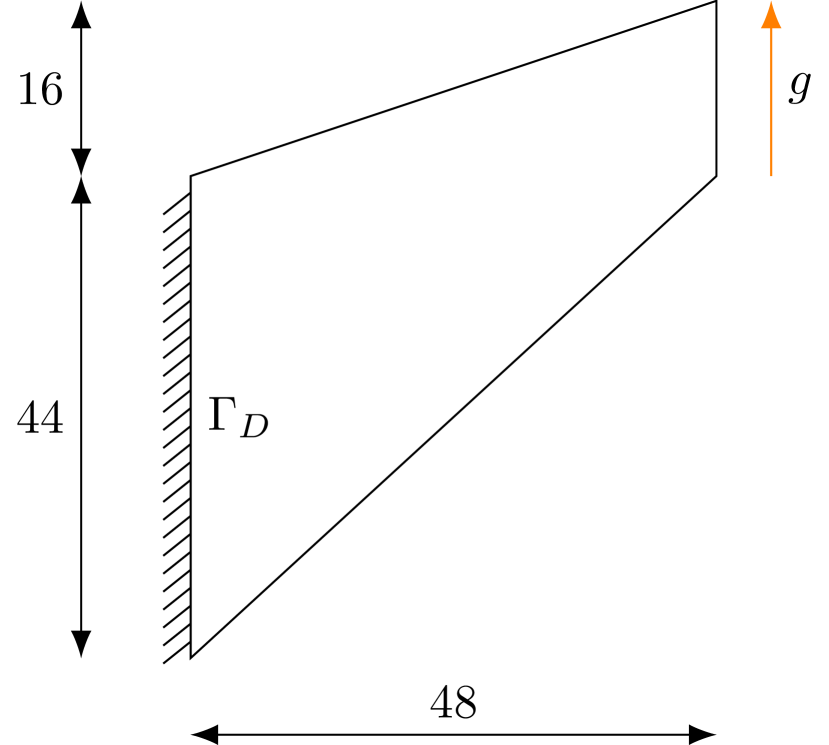
Figure 5. Computational domain and absolute value of the displacement on the adaptively refined triangulation of example 7.2 using the SGG2 element.

Figure 6. Convergence of the error estimator $\eta$ for example 7.2.

7.3. Clamped Fichera corner

Wo consider a clamped Fichera corner example. The geometry is given by $\Omega=(-1,1)^{3}\setminus(0,1)^{3}$ and we choose the parameters $E=1$ and $\nu=0.3$. We consider the object to be clamped at $x=-1$ and apply a traction force $g=(0,0,-10^{-3})$ on the opposite side where $x=1$. All other boundaries are free (i.e. $g=0$). In contrast to the two dimensional setting the solution now includes vertex and edge singularities, i.e. even for an adaptively refined triangulation we might not see the "optimal" convergence if we do not apply an anisotropic refinement strategy, see [2]. Since this is out of scope of this work we applied the same adaptive refinement as for the other examples. In Figure 7 we have plotted the absolute value of the displacement using the SGG2 finite element and deformed the geometry with a scaling factor of 20 since otherwise the deformation would not be visible. In addition we show the adaptively refined triangulation (from the last step). One can clearly see that the estimator successfully detects the edge and vertex singularities i.e. that the corresponding elements are marked and refined during the computation loop. In Figure 8 we plot the estimator $\eta$ for the SGG2 and the RAFW element using an adaptive refinement and included also the convergence using a uniform refinement for the RAFW element. Although we do not see the optimal convergence (as noted above) we still see the drastic decrease in the error when using an adaptive mesh refinement.

Figure 7. Absolute value of the displacement on the deformed adaptively refined triangulation of example 7.3 using the SGG2 element.

Figure 8. Convergence of the error estimator $\eta$ for example 7.3

References

- [1] M. Amara and J. M. Thomas. Equilibrium finite elements for the linear elastic problem. Numer. Math., 33(4):367–383, 1979.
- [2] Thomas Apel. Anisotropic finite elements: local estimates and applications. Advances in Numerical Mathematics. B. G. Teubner, Stuttgart, 1999.
- [3] D. N. Arnold and F. Brezzi. Mixed and nonconforming finite element methods: implementation, postprocessing and error estimates. RAIRO Modél. Math. Anal. Numér., 19(1):7–32, 1985.
- [4] Douglas N. Arnold, Gerard Awanou, and Ragnar Winther. Finite elements for symmetric tensors in three dimensions. Math. Comp., 77(263):1229–1251, 2008.
- [5] Douglas N. Arnold, Franco Brezzi, and Jim Douglas, Jr. PEERS: a new mixed finite element for plane elasticity. Japan J. Appl. Math., 1(2):347–367, 1984.
- [6] Douglas N. Arnold, Jim Douglas, Jr., and Chaitan P. Gupta. A family of higher order mixed finite element methods for plane elasticity. Numer. Math., 45(1):1–22, 1984.
- [7] Douglas N. Arnold, Richard S. Falk, and Ragnar Winther. Differential complexes and stability of finite element methods. II. The elasticity complex. In Compatible spatial discretizations, volume 142 of IMA Vol. Math. Appl., pages 47–67. Springer, New York, 2006.
- [8] Douglas N. Arnold, Richard S. Falk, and Ragnar Winther. Finite element exterior calculus, homological techniques, and applications. Acta Numer., 15:1–155, 2006.
- [9] Douglas N. Arnold, Richard S. Falk, and Ragnar Winther. Mixed finite element methods for linear elasticity with weakly imposed symmetry. Math. Comp., 76(260):1699–1723 (electronic), 2007.
- [10] Ivo Babuška and Manil Suri. Locking effects in the finite element approximation of elasticity problems. Numer. Math., 62(4):439–463, 1992.
- [11] Daniele Boffi, Franco Brezzi, and Michel Fortin. Mixed finite element methods and applications, volume 44 of Springer Series in Computational Mathematics. Springer, Heidelberg, 2013.
- [12] Susanne C. Brenner. Korn’s inequalities for piecewise vector fields. Math. Comp., 73(247):1067–1087, 2004.
- [13] C. Carstensen, G. Dolzmann, S. A. Funken, and D. S. Helm. Locking-free adaptive mixed finite element methods in linear elasticity. Comput. Methods Appl. Mech. Engrg., 190(13-14):1701–1718, 2000.
- [14] Carsten Carstensen and Georg Dolzmann. A posteriori error estimates for mixed FEM in elasticity. Numer. Math., 81(2):187–209, 1998.
- [15] Bernardo Cockburn, Jayadeep Gopalakrishnan, and Johnny Guzmán. A new elasticity element made for enforcing weak stress symmetry. Math. Comp., 79(271):1331–1349, 2010.
- [16] Daniele Antonio Di Pietro and Alexandre Ern. Mathematical aspects of discontinuous Galerkin methods, volume 69 of Mathématiques & Applications (Berlin) [Mathematics & Applications]. Springer, Heidelberg, 2012.
- [17] B. M. Fraeijs de Veubeke. Discretization of rotational equilibrium in the finite element method. In Mathematical aspects of finite element methods (Proc. Conf., Consiglio Naz. delle Ricerche (C.N.R.), Rome, 1975), pages 87–112. Lecture Notes in Math., Vol. 606. Springer, Berlin, 1977.
- [18] B. M. Fraeijs de Veubeke and A. Millard. Discretization of stress fields in the finite element method. J. Franklin Inst., 302(5-6):389–412, 1976. Basis of the finite element method.
- [19] B.M. Fraejis de Veubeke. Displacement and equilibrium models in the finite element method. In O.C Zienkiewics and G.S. Holister, editors, Stress analysis, pages 145–197. Wiley, 1965.
- [20] B.M. Fraejis de Veubeke. Stress function approach. Proc. of the World Congress on Finite Element Methods in Structural Mechanics, Vol. 1. Dorset, England (Oct. 12-17, 1975):J.1–J.51, 1975.
- [21] Vivette Girault and Pierre-Arnaud Raviart. Finite element methods for Navier-Stokes equations, volume 5 of Springer Series in Computational Mathematics. Springer-Verlag, Berlin, 1986. Theory and algorithms.
- [22] J. Gopalakrishnan and J. Guzmán. A second elasticity element using the matrix bubble. IMA J. Numer. Anal., 32(1):352–372, 2012.
- [23] Johnny Guzmán and Michael Neilan. Symmetric and conforming mixed finite elements for plane elasticity using rational bubble functions. Numer. Math., 126(1):153–171, 2014.
- [24] Antti Hannukainen, Rolf Stenberg, and Martin Vohralík. A unified framework for a posteriori error estimation for the Stokes problem. Numer. Math., 122(4):725–769, 2012.
- [25] C. Johnson and B. Mercier. Some equilibrium finite element methods for two-dimensional elasticity problems. Numer. Math., 30(1):103–116, 1978.
- [26] Kwang-Yeon Kim. Guaranteed a posteriori error estimator for mixed finite element methods of linear elasticity with weak stress symmetry. SIAM J. Numer. Anal., 49(6):2364–2385, 2011.
- [27] Philip L. Lederer and Rolf Stenberg. Energy norm analysis of exactly symmetric mixed finite elements for linear elasticity, 2021.
- [28] Marco Lonsing and Rüdiger Verfürth. A posteriori error estimators for mixed finite element methods in linear elasticity. Numer. Math., 97(4):757–778, 2004.
- [29] Jindřich Nečas and Ivan Hlaváček. Mathematical theory of elastic and elasto-plastic bodies: an introduction, volume 3 of Studies in Applied Mechanics. Elsevier Scientific Publishing Co., Amsterdam-New York, 1980.
- [30] W. Prager and J. L. Synge. Approximations in elasticity based on the concept of function space. Quart. Appl. Math., 5:241–269, 1947.
- [31] J. Schöberl. NETGEN An advancing front 2D/3D-mesh generator based on abstract rules. Computing and Visualization in Science, 1(1):41–52, 1997.
- [32] L. R. Scott and M. Vogelius. Norm estimates for a maximal right inverse of the divergence operator in spaces of piecewise polynomials. RAIRO Modél. Math. Anal. Numér., 19(1):111–143, 1985.
- [33] Rolf Stenberg. A family of mixed finite elements for the elasticity problem. Numer. Math., 53(5):513–538, 1988.
- [34] Rolf Stenberg. Some new families of finite elements for the Stokes equations. Numer. Math., 56(8):827–838, 1990.
- [35] Rolf Stenberg. Postprocessing schemes for some mixed finite elements. RAIRO Modél. Math. Anal. Numér., 25(1):151–167, 1991.
- [36] B. A. Szabó and I. Babuška. Finite Element Analysis. A Wiley-Interscience publication. Wiley, 1991.
- [37] Rüdiger Verfürth. A posteriori error estimation techniques for finite element methods. Numerical Mathematics and Scientific Computation. Oxford University Press, Oxford, 2013.