Information geometry of excess and housekeeping entropy production

Abstract

A nonequilibrium system is characterized by a set of thermodynamic forces and fluxes which give rise to entropy production (EP). We show that these forces and fluxes have an information-geometric structure, which allows us to decompose EP into contributions from different types of forces in general (linear and nonlinear) discrete systems. We focus on the excess and housekeeping decomposition, which separates contributions from conservative and nonconservative forces. Unlike the Hatano-Sasa decomposition, our housekeeping/excess terms are always well-defined, including in systems with odd variables and nonlinear systems without steady states. Our decomposition leads to far-from-equilibrium thermodynamic uncertainty relations and speed limits. As an illustration, we derive a thermodynamic bound on the time necessary for one cycle in a chemical oscillator.

A major goal of nonequilibrium thermodynamics is to understand entropy production (EP) from an operational point of view, in terms of tradeoffs between EP and functional properties such as speed of dynamical evolution (aurell2011optimal, ; shiraishi_speed_2018, ) and statistics of fluctuating observables (gingrich2016dissipation, ). However, EP can arise from different factors, including relaxation from nonequilibrium states, nonconservative forces, and exchange of conserved quantities between different reservoirs. In this Letter, we use methods from information geometry (amari2016information, ; ay2017information, ) to decompose EP into nonnegative contributions from different sources and to study their operational consequences.

We focus on the decomposition of EP into excess and housekeeping terms (esposito2010three, ; hatano2001steady, ; oono1998steady, ). At a general level, excess EP is the contribution from conservative forces, which arise from the change of a thermodynamic potential, and it is expected to vanish in steady state. Housekeeping EP is the contribution from nonconservative forces, such as the forces that generate cyclic fluxes in nonequilibrium steady states. The housekeeping contribution can be arbitrarily large, and in general it diverges during quasistatic transformations between nonequilibrium steady states (mandal2016analysis, ; maes2014nonequilibrium, ). One of the main goals of this decomposition is to derive tighter thermodynamic tradeoffs and bounds by considering only the excess part of EP (oono1998steady, ; maes2014nonequilibrium, ).

While the housekeeping/excess decomposition is well understood at a conceptual level, identifying the correct formal definitions remains an open area of research (komatsu2008steady, ; spinney2012nonequilibrium, ; lee2013fluctuation, ; maes2014nonequilibrium, ; kohei2022, ; sagawa2011geometrical, ). The best known proposal is the Hatano-Sasa (HS) decomposition, also called the adiabatic/nonadiabatic decomposition (hatano2001steady, ; esposito2010three, ; esposito2007entropy, ; rao2016nonequilibrium, ; ge2016nonequilibrium, ). However, the HS decomposition has several drawbacks. First, its physical meaning in terms of experimentally accessible observables is unclear (dechant2022geometric, ; dechant2022geometricCoupling, ; maes2014nonequilibrium, ). Second, it can lead to unphysical negative values in stochastic systems with odd variables (variables such as velocity whose sign changes under time-reversal) (ford2012entropy, ; spinney2012nonequilibrium, ; lee2013fluctuation, ). It can also lead to negative values in chemical systems that violate complex balance (rao2016nonequilibrium, ; ge2016nonequilibrium, ). Finally, it is unclear how to define the HS decomposition for systems that lack stable steady states, such as chemical systems that exhibit oscillations (kohei2022, ). These drawbacks suggest that the HS decomposition is not the ultimate definition of excess and housekeeping EP.

Here we propose a new excess/housekeeping decomposition which resolves all of these issues. Our decomposition is derived using techniques from information geometry, and it is well-defined and nonnegative for all discrete systems, including systems with odd variables and nonlinear chemical systems without steady states. Our excess EP is experimentally accessible via statistics of fluctuating observables, and it leads to new thermodynamic uncertainty relations (TURs) and thermodynamic speed limits (TSLs), which can be tight even in the far-from-equilibrium regime.

Our approach is related to the decomposition proposed by Maes and Netočný (MN) for Langevin systems (maes2014nonequilibrium, ), which is recovered in the appropriate continuum limit. The MN decomposition was studied from a geometric perspective in Refs. (nakazato2021geometrical, ; dechant2022geometric, ; dechant2022geometricCoupling, ), and generalized to discrete systems by the present authors in Ref. (kohei2022, ). Unlike these previous papers, which used a generalized Euclidean geometry, here we consider the non-Euclidean setting of information geometry, which is more appropriate for far-from-equilibrium systems (for a comparison with Ref. (kohei2022, ), see  SM7.2 in the Supplemental Material (SM).).

This work complements existing research on geometry and thermodynamics (weinhold_metric_1975, ; ruppeiner_thermodynamics_1979, ; salamon_thermodynamic_1983, ; schlogl_thermodynamic_1985, ; janyszek_riemannian_1990, ; diosi_thermodynamic_1996, ), including recent studies of stochastic thermodynamics and information geometry mrugala_statistical_1990 ; brody_geometrical_1995 ; crooks_measuring_2007 ; sivak_thermodynamic_2012 ; ito2018stochastic ; nakamura2019reconsideration ; ito2020stochastic ; ito2022information ; kolchinsky2021work ; yoshimura2021information ; ohga2021information1 ; sughiyama2021hessian ; ohga2021information ; kobayashi2021kinetic ; nicholson2018nonequilibrium ; shiraishi2019information ; van2021geometrical . However, almost all of these studies considered the geometry of thermodynamic states, rather than dynamical quantities (thermodynamic forces and fluxes) as pursued here. Exceptions include Ref. (ito2020unified, ), which studied information geometry of trajectories in stochastic systems, but did not derive decompositions based on constraints on forces nor analyze their operational implications. Finally, Ref. (Kobayashi2022, ) recently considered decompositions of fluxes and forces using different type of information geometry (see SM7.3 for a summary and comparison).

Setup.— We consider a system with $N$ species or states with distribution $\bm{p}=(p_{1},\dots,p_{N})\in\mathbb{R}_{>0}^{N}$ at time $t$. The system evolves in continuous time, either as a linear stochastic master equation or a nonlinear rate equation (deterministic chemical reaction system). The dynamics are generated by a set of $M$ reversible reactions, where each reaction $\rho\in\{1..M\}$ is associated with a unique reverse reaction $\tilde{\rho}\in\{1..M\}$. The reactions are also associated with a set of (one-way) fluxes $\bm{J}=(J_{1},\dots,J_{M})\in\mathbb{R}_{>0}^{M}$. Note that $\bm{p}$ and $\bm{J}$ generally depend on time, though we leave this dependence implicit in the notation. We make no assumptions about the form of the fluxes (e.g., no assumption of mass action kinetics), except where otherwise noted.

For each reaction $\rho$ and species $x$, the stoichiometric coefficient $\nabla_{\rho x}=-\nabla_{\tilde{\rho}x}\in\mathbb{Z}$ indicates how many units of $x$ are added or removed by $\rho$. The overall matrix $\nabla\in\mathbb{Z}^{M\times N}$ acts the discrete gradient operator: for any state observable $\bm{\phi}\in\mathbb{R}^{N}$, $[\nabla\bm{\phi}]_{\rho}$ indicates how much reaction $\rho$ changes the amount of $\bm{\phi}$. Its transpose $\nabla^{T}$ acts as the (negative) discrete divergence operator. The system’s distribution evolves according to the continuity equation $\mathrm{d}_{t}\bm{p}=\nabla^{T}\bm{J}$, while expectations of observables evolve as $(\mathrm{d}_{t}\bm{p})^{T}\bm{\phi}=\bm{J}^{T}\nabla\bm{\phi}$.

The reactions are also associated with a set of thermodynamic forces $\bm{f}=(f_{1},\dots,f_{M})\in\mathbb{R}^{M}$ which we assume obey local detailed balance. For now, we restrict our attention to systems without odd variables, in which case the forces are given by the log ratio of forward and reverse fluxes, $f_{\rho}=\ln(J_{\rho}/J_{\tilde{\rho}})$. Note that $f_{\rho}$ is the change in total entropy due to reaction $\rho$ and the entropy production rate (EPR) is given by $\dot{\sigma}=\sum_{\rho}J_{\rho}f_{\rho}=\sum_{\rho}J_{\rho}\ln(J_{\rho}/J_{\tilde{\rho}})$.

To make things concrete, consider a stochastic master equation without odd variables. Here $\bm{p}$ is a probability distribution which evolves as $\mathrm{d}_{t}p_{x}=\sum_{y(\neq x),\alpha}(p_{y}R_{xy}^{\alpha}-p_{x}R_{yx}^{\alpha})$, where $R_{yx}^{\alpha}$ is the rate of transitions $x\shortrightarrow y$ mediated by reservoir $\alpha$. Each “reaction” $\rho$ represents one transition $(x\shortrightarrow y,\alpha)$ with flux $J_{\rho}=p_{x}R_{yx}^{\alpha}$, stoichiometry $\nabla_{\rho z}=\delta_{zy}-\delta_{zx}$ (so that $[\nabla\bm{\phi}]_{\rho}=\phi_{y}-\phi_{x}$), and reverse reaction $\tilde{\rho}$ corresponding to the transition $(y\shortrightarrow x,\alpha)$.

Alternatively, for deterministic chemical systems, $\bm{p}$ is a vector of nonnegative concentrations of different chemical species, $\nabla$ is the transpose of the stoichiometric matrix, and $\bm{J}$ is the vector of fluxes across reversible reactions (see SM1 for more details of chemical systems, including a generalization of our formalism to account for external currents).

To introduce techniques from information geometry, we define an exponential family of fluxes parameterized by $\bm{\theta}\in\mathbb{R}^{M}$:

$$j_{\rho}(\bm{\theta}):=J_{\rho}e^{\theta_{\rho}-f_{\rho}}.$$ (1)

Within this family, the actual fluxes are recovered at $\bm{\theta}=\bm{f}$, $J_{\rho}=j_{\rho}(\bm{f})$, and the reverse fluxes are recovered at $\bm{\theta}=\bm{0}$, $J_{\tilde{\rho}}=j_{\rho}(\bm{0})$. The generalized Kullback-Leibler (KL) divergence (Def. 2.8, ay2017information, ) provides an information-theoretic distance between members of this family:

$$\mathcal{D}(\bm{\theta}\|\bm{\theta}^{\prime})=\sum_{\rho}\Big{[}j_{\rho}(\bm{\theta})\ln\frac{j_{\rho}(\bm{\theta})}{j_{\rho}(\bm{\theta}^{\prime})}+j_{\rho}(\bm{\theta}^{\prime})-j_{\rho}(\bm{\theta})\Big{]}\geq 0.$$ (2)

Importantly, the EPR can be written using this KL divergence,

$$\dot{\sigma}=\mathcal{D}(\bm{f}\|\bm{0}),$$ (3)

which follows from Eqs. (1)-(2) and $\sum_{\rho}J_{\rho}=\sum_{\rho}J_{\tilde{\rho}}$.

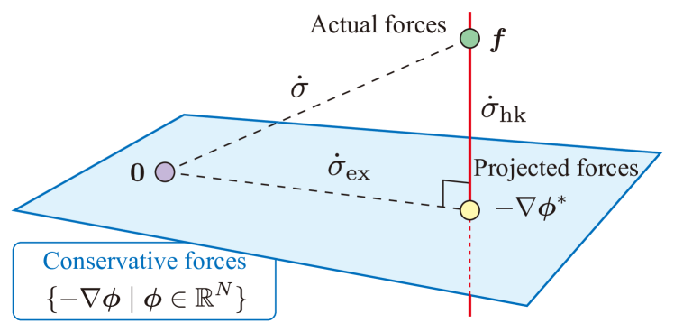
Figure 1: Illustration of excess/housekeeping decomposition, Eq. 6. The red line indicates the set of parameter values that lead to the same dynamical evolution as the forward fluxes, $\bm{j}(\bm{\theta})=\nabla\bm{j}(\bm{f})=\nabla\bm{J}$.

Housekeeping vs. excess EPR.— We now introduce our decomposition of the EPR, which is shown visually in Fig. 1. Derivations of these results, which use standard techniques from information geometry, are in SM2.

Recall that a vector of thermodynamic forces $\bm{f}$ is called conservative if it is the negative gradient of some thermodynamic potential $\bm{\phi}\in\mathbb{R}^{N}$, so that $\bm{f}={-\nabla}\bm{\phi}$. For example, for a master equation that obeys detailed balance relative to an equilibrium distribution $\bm{\pi}$ ($R_{xy}\pi_{y}=R_{yx}\pi_{x}$), the thermodynamic forces are conservative for the potential $\phi_{x}=\ln(p_{x}/\pi_{x})$.

In general, the housekeeping EPR should vanish when $\bm{f}$ is conservative. Motivated by this, we define the housekeeping EPR as the information-theoretic distance between $\bm{f}$ and the closest conservative force ${-\nabla}\bm{\phi}$,

$$\dot{\sigma}_{\text{hk}}:=\min_{\bm{\phi}\in\mathbb{R}^{N}}\mathcal{D}(\bm{f}\|{-\nabla}\bm{\phi})\geq 0.$$ (4)

Note that $0\leq\dot{\sigma}_{\text{hk}}\leq\dot{\sigma}$, since $\mathcal{D}$ is nonnegative and $\mathcal{D}(\bm{f}\|\bm{0})=\dot{\sigma}$ is achieved by $\bm{\phi}=\bm{0}$. Furthermore, the minimum is always achieved by some optimal potential $\bm{\phi}^{*}$, and the optimal conservative force ${-\nabla}\bm{\phi}^{*}$ is unique (SM2.1). Therefore, when $\bm{f}$ is conservative, $\dot{\sigma}_{\text{hk}}$ vanishes and ${-\nabla}\bm{\phi}^{*}=\bm{f}$.

The excess EPR is defined as the remainder $\dot{\sigma}_{\text{ex}}:=\dot{\sigma}-\dot{\sigma}_{\text{hk}}$. Using the duality principle from information geometry, $\dot{\sigma}_{\text{ex}}$ can be written in a variational form (SM2.2),

$$\dot{\sigma}_{\text{ex}}=\min_{\bm{\theta}\in\mathbb{R}^{M}}\mathcal{D}(\bm{\theta}\|\bm{0})\quad\text{where}\quad\nabla^{T}\bm{j}(\bm{\theta})=\mathrm{d}_{t}\bm{p}.$$ (5)

This means that $\dot{\sigma}_{\text{ex}}$ is the distance from the closest $\bm{j}(\bm{\theta})$ to the reverse fluxes $\bm{j}(\bm{0})$ such that $\bm{j}(\bm{\theta})$ leads to the same dynamical evolution as the actual fluxes, $\mathrm{d}_{t}\bm{p}=\nabla^{T}\bm{J}$. The optimum is achieved by the optimal conservative force ${-\nabla}\bm{\phi}^{*}$ in Eq. 4. Both Eqs. 4 and 5 are convex optimization problems that can be solved using standard numerical techniques.

Combining these results, we can write our decomposition using the Pythagorean relation for KL divergence (see Fig. 1):

$$\underbrace{\mathcal{D}(\bm{f}\|\bm{0})}_{\begin{matrix}\dot{\sigma}\end{matrix}}=\underbrace{\mathcal{D}(\bm{f}\|{-\nabla}\bm{\phi}^{*})}_{\begin{matrix}\dot{\sigma}_{\text{hk}}\end{matrix}}+\underbrace{\mathcal{D}({-\nabla}\bm{\phi}^{*}\|\bm{0})}_{\begin{matrix}\dot{\sigma}_{\text{ex}}\end{matrix}}.$$ (6)

Eq. 6 is analogous to the Pythagorean Theorem in Euclidean geometry, with the KL divergence playing the role of squared Euclidean distance.

The optimal potential $\bm{\phi}^{*}$ has several interesting properties. Given Eq. 5, the fluxes corresponding to the optimal conservative force ${-\nabla}\bm{\phi}^{*}$ give rise to the actual dynamical evolution, $\mathrm{d}_{t}\bm{p}=\nabla^{T}\bm{j}({-\nabla}\bm{\phi}^{*})$. Moreover, as we show in SM4, this dynamical evolution can be written as a gradient flow for a free energy defined in terms of $\bm{\phi}^{*}$, which generalizes an existing result for conservative forces (maas_gradient_2011, ; mielke2011gradient, ). In essence, $\bm{\phi}^{*}$ acts as the system’s “effective” free energy, which is well-defined even in the presence of nonconservative forces.

Although the definition of $\dot{\sigma}_{\text{ex}}$ makes no explicit mention of steady state, $\dot{\sigma}_{\text{ex}}$ vanishes if the system is in steady state (SM2.5). Note that the reverse fluxes induce the opposite dynamics as the forward fluxes, $\nabla\bm{j}(\bm{0})=-\nabla\bm{J}$. In steady state, $\mathrm{d}_{t}\bm{p}=\nabla\bm{J}=\bm{0}$, so the reverse fluxes satisfy the constraint in Eq. 5, $\nabla^{T}\bm{j}(\bm{0})=\bm{0}$, while achieving the minimum $\dot{\sigma}_{\text{ex}}=0$. In addition, by properties of KL divergence, $\dot{\sigma}_{\text{ex}}\sim\|\mathrm{d}_{t}\bm{p}\|^{2}$ near steady state. Thus, the time integral of excess EP vanishes in the quasistatic limit of slow driving, when $\tau\to\infty$ and $\mathrm{d}_{t}\bm{p}\sim 1/\tau$.

We can compare our decomposition to the HS decomposition. For stochastic master equations, the HS housekeeping EPR can be expressed as the information-theoretic distance between $\bm{f}$ and a particular vector of conservative forces, $\dot{\sigma}_{\text{hk}}^{\text{HS}}=\mathcal{D}(\bm{f}\|{-\nabla}\bm{\phi}^{\mathrm{ss}})$, where the potential $\phi_{x}^{\mathrm{ss}}=\ln p_{x}/\pi_{x}^{\mathrm{ss}}$ is defined via the steady-state distribution $\bm{\pi}^{\mathrm{ss}}$ (SM7.1). The same result also holds for nonlinear chemical systems with mass action kinetics and complex balance. The variational principle in Eq. 4 then implies that $\dot{\sigma}_{\text{hk}}\leq\dot{\sigma}_{\text{hk}}^{\text{HS}}$ and $\dot{\sigma}_{\text{ex}}\geq\dot{\sigma}_{\text{ex}}^{\text{HS}}$. The remainder $\dot{\sigma}_{\text{cpl}}=\dot{\sigma}_{\text{hk}}^{\text{HS}}-\dot{\sigma}_{\text{hk}}\geq 0$ is a “coupling term”, similar to one recently proposed for Langevin dynamics (dechant2022geometricCoupling, ).

Importantly, our general approach can be used to derive many other kinds of decomposition of the EPR, not just the housekeeping/excess decomposition. By replacing $\nabla$ with some other matrix in Eq. 4, one can consider projections onto a different subspace of forces, rather than the set of conservative forces. We leave exploration of such alternative decompositions for future work.

Excess EPR and dynamical fluctuations.— Our housekeeping/excess decomposition is directly related to the dynamical fluctuations of observables, which provides an effective way to bound and estimate $\dot{\sigma}_{\text{ex}}$ from experimental data. This differs from the existing decompositions, including the HS decomposition, which requires knowledge of the steady state and has no direct relationship with physical observables at a given point in time (dechant2022geometric, ).

Let us first review the relationship between dynamical fluctuations and the EPR. It has been recently shown that the EPR obeys the following variational principle (kim2020learning, ; otsubo2020estimating, ) (SM2.4):

$$\dot{\sigma}=\max_{\bm{\theta}\in\Theta}\sum_{\rho}J_{\rho}(\theta_{\rho}-e^{-\theta_{\rho}}+1),$$ (7)

where $\Theta=\{\bm{\theta}\in\mathbb{R}^{M}:\theta_{\rho}=\theta_{\tilde{\rho}}\,\forall\rho\}$ is the set of antisymmetric current observables, and the maximum is achieved by the thermodynamic forces $\bm{f}$. A series expansion gives $\dot{\sigma}=\max_{\bm{\theta}\in\Theta}[2\langle\bm{\theta}\rangle-\sum_{k>1}(-1)^{k}\langle\bm{\theta}^{k}\rangle/k!]$, where $\langle\bm{\theta}^{k}\rangle=\bm{J}^{T}\bm{\theta}^{k}$ is the $k$th moment of $\bm{\theta}$. Thus, in stochastic systems, EPR constrains the mean and higher-order fluctuations of all current observables. This constraint is stronger than standard TURs (van2020entropy, ), because the maximum in Eq. 7 always gives the exact EPR, including in discrete systems and systems arbitrarily far from equilibrium and steady state. This provides a powerful method for measuring EPR from empirical observations (kim2020learning, ; otsubo2020estimating, ), since any choice of current observable gives a bound on the EPR which can be made arbitrarily tight by optimizing over observables.

Our decomposition has a closely related interpretation. Specifically, excess EPR can be written in terms of the following variational formula,

$$\dot{\sigma}_{\text{ex}}=\max_{\bm{\phi}\in\mathbb{R}^{N}}\sum_{\rho}J_{\rho}([{-\nabla}\bm{\phi}]_{\rho}-e^{[\nabla\bm{\phi}]_{\rho}}+1),$$ (8)

where the $\bm{\phi}$ that achieves the maximum is the optimal potential $\bm{\phi}^{*}$ from Eq. 4. Eq. 8 follows from $\dot{\sigma}_{\text{ex}}=\mathcal{D}(\bm{f}\|\bm{0})-\min_{\bm{\phi}}\mathcal{D}(\bm{f}\|{-\nabla}\bm{\phi})$ and rearranging (SM2.4).

This shows that $\dot{\sigma}_{\text{ex}}$ satisfies the same variational principle as the EPR, except that current observables are restricted to those of the form ${-\nabla}\bm{\phi}$, as generated by the change of some state observable $\bm{\phi}$. (We use the symbol $\bm{\phi}$ for both state potentials and state observables, since they are not formally distinguished in our approach.) Thus, in stochastic systems, $\dot{\sigma}_{\text{ex}}$ constrains the dynamic fluctuations of all state observables; conversely, $\dot{\sigma}_{\text{ex}}$ is the part of EPR that can be accessed by measuring the fluctuations of state observables. The same techniques proposed in (kim2020learning, ; otsubo2020estimating, ) to estimate EPR can also be used to estimate excess EPR from real-world data. In fact, it may be much easier to estimate $\dot{\sigma}_{\text{ex}}$ than $\dot{\sigma}$, since $\dot{\sigma}_{\text{ex}}$ does not require measurements of arbitrary current observables but only changes of state observables (i.e., by measuring some $\bm{\phi}$ at time $t$ and $t+\delta t$ over many runs of a process).

For a system governed by conservative forces, $\dot{\sigma}=\dot{\sigma}_{\text{ex}}$ and the two variational principles in Eqs. 7 and 8 agree. In fact, for stochastic master equations with conservative forces, Ref. (shiraishi2019information, ) derived a variational expression of $\dot{\sigma}$ that turns out to be equivalent to Eq. 8. Our decomposition generalizes that variational principle to linear and nonlinear systems with nonconservative forces. It also generalizes the main result of Ref. (shiraishi2019information, ), which is an information-theoretic bound on the speed of evolution in stochastic equations with time-symmetric driving (SM3).

TURs and TSLs.— We now use Eq. 8 to derive TURs and TSLs for the excess EP. Our results apply both to linear and nonlinear systems.

Consider any state observable $\bm{\phi}$, and assume without loss of generality that it is scaled so that $\left\|\nabla\bm{\phi}(t)\right\|_{\infty}\leq 1$. Our bounds are stated in terms of the observable’s speed $\mathcal{J}_{\bm{\phi}}:=\sum_{\rho}J_{\rho}[\nabla\bm{\phi}]_{\rho}=(\mathrm{d}_{t}\bm{p})^{T}\bm{\phi}$ and the dynamical activity $A=\sum_{\rho}J_{\rho}$ (the overall number of reactions per second (shiraishi_speed_2018, )). We also consider the “mean deviation” of the observable’s dynamic fluctuations, $\mathcal{V}_{\bm{\phi}}=\sum_{\rho}J_{\rho}|[\nabla\bm{\phi}]_{\rho}|\leq A$. $\mathcal{V}_{\bm{\phi}}$ is a nonnegative measure of the size of fluctuations that vanishes when $\bm{\phi}$ is a conserved quantity.

We first derive the following short-time TUR,

$$\dot{\sigma}_{\text{ex}}\geq 2\mathcal{J}_{\bm{\phi}}\,\tanh^{-1}\frac{\mathcal{J}_{\bm{\phi}}}{\mathcal{V}_{\bm{\phi}}}\geq 2\mathcal{J}_{\bm{\phi}}\,\tanh^{-1}\frac{\mathcal{J}_{\bm{\phi}}}{A}.$$ (9)

This result follows from Eq. 8 and a simple bound on the exponential function, with all details in SM5. We can also derive a finite-time version of Eq. 9. We consider a process over time $t\in[0,\tau]$ and any time-dependent observable $\bm{\phi}(t)$ ($\left\|\nabla\bm{\phi}(t)\right\|_{\infty}\leq 1$ at all $t$). Using Eq. 9 and Jensen’s inequality, we derive a bound on the integrated excess EP $\Sigma_{\mathrm{ex}}(\tau)=\int_{0}^{\tau}\dot{\sigma}_{\text{ex}}(t)\,dt$,

$$\Sigma_{\mathrm{ex}}(\tau)\geq 2\mathcal{L}_{\bm{\phi}}\,\tanh^{-1}\frac{\mathcal{L}_{\bm{\phi}}}{\tau\langle\mathcal{V}_{\bm{\phi}}\rangle}\geq 2\mathcal{L}_{\bm{\phi}}\,\tanh^{-1}\frac{\mathcal{L}_{\bm{\phi}}}{\tau\langle A\rangle},$$ (10)

where $\mathcal{L}_{\bm{\phi}}=\int_{0}^{\tau}|\mathcal{J}_{\bm{\phi}}(t)|\,dt$ is the trajectory length of the observable, while $\langle\mathcal{V}_{\bm{\phi}}\rangle=(1/\tau)\int_{0}^{\tau}\mathcal{V}_{\bm{\phi}}(t)\,dt$ and $\langle A\rangle=(1/\tau)\int_{0}^{\tau}\sum_{\rho}J_{\rho}(t)\,dt$ are time-averaged mean deviation and dynamical activity. A simple rearrangement of Eq. 10 gives a far-from-equilibrium TSL:

$$\tau\geq\frac{\mathcal{L}_{\bm{\phi}}}{\langle\mathcal{V}_{\bm{\phi}}\rangle}\coth\frac{\Sigma_{\mathrm{ex}}}{2\mathcal{L}_{\bm{\phi}}}\geq\frac{\mathcal{L}_{\bm{\phi}}}{\langle A\rangle}\coth\frac{\Sigma_{\mathrm{ex}}}{2\mathcal{L}_{\bm{\phi}}}.$$ (11)

Naturally, these bounds also hold for total EP, $\Sigma_{\mathrm{ex}}\leq\Sigma$.

The choice of the time-dependent observable in Eqs. 10 and 11 can be used to derive various specialized TSLs. For example, for the “total variation” observable $\phi_{x}^{\mathrm{tv}}(t):=(1/2)\mathrm{sign}(\mathrm{d}_{t}p_{x}(t))$, the trajectory length is $\mathcal{L}_{\bm{\phi}^{\mathrm{tv}}}=(1/2)\int_{0}^{\tau}\left\|\mathrm{d}_{t}\bm{p}\right\|_{1}\,dt$. Alternatively, using a different time-dependent observable, one can derive TSLs for the “$L_{1}$-Wasserstein path length”, an important quantity in optimal transport theory (see (Sec. 4, dechant2022minimum, ) for details).

The bound in Eq. 9 diverges as $\mathcal{J}_{\bm{\phi}}/A\to 1$, the absolutely irreversible regime where all activity is channeled into directed movement. It is stronger than conventional TURs that are quadratic in $\mathcal{J}_{\bm{\phi}}$ (horowitz2020thermodynamic, ), which are tight only near equilibrium and do not diverge in the limit of absolute irreversibility. Furthermore, Eq. 11 implies a finite minimal time $\tau_{\mathrm{min}}=\mathcal{L}/\langle A\rangle$, where $\Sigma_{\mathrm{ex}}$ diverges as $-\ln(\tau-\tau_{\mathrm{min}})$ as $\tau\to\tau_{\min}$. This is stronger than the $1/\tau$ finite-time scaling reported in conventional TSLs (aurell2011optimal, ; shiraishi_speed_2018, ; van2021geometrical, ; nakazato2021geometrical, ; yoshimura2021thermodynamic, ; hamazaki2022speed, ; kohei2022, ), which only become tight in the limit of slow driving (berut2012experimental, ; zhen2021universal, ; zhen2022inverse, ). The difference between these finite-time scaling relations is shown in Fig. 2(a). Our bounds can be related to recently proposed far-from-equilibrium TURs (delvenne2021thermo, ; van2020unifiedCSLTUR, ) and TSLs (dechant2022minimum, ; lee2022speed, ; salazar2022lower, ) but go beyond these existing results, which either do not apply to nonlinear chemical systems and/or do not separately consider excess EP (therefore cannot be tight in the presence of nonconservative forces).

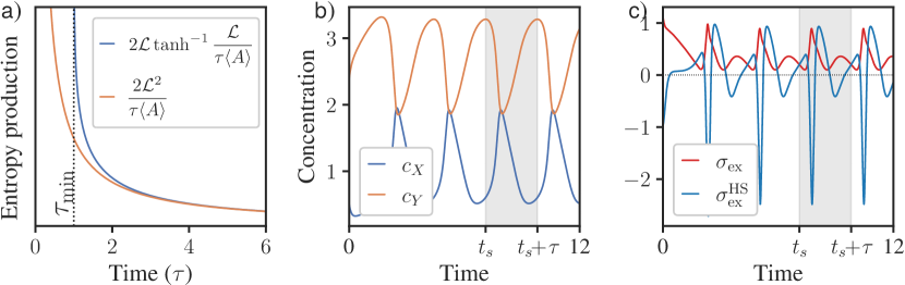
Figure 2: a) Finite-time scaling in Eq. 10 vs. $1/\tau$ scaling in standard TSLs. b) Trajectory of a Brusselator model that reaches a limit cycle. We derive a bound on the minimal time $\tau$ need to complete a cycle. c) $\dot{\sigma}_{\text{ex}}(t)$ vs. $\dot{\sigma}_{\text{ex}}^{\text{HS}}(t)$ for the Brusselator model.

Example.— We illustrate our results on the Brusselator prigogine1968symmetry , a well-known model of an autocatalytic chemical system. The model contains three reactions: 1) $\varnothing\rightleftarrows X$, 2) $X\rightleftarrows Y$, and 3) $2X+Y\rightleftarrows 3X$. We assume mass action kinetics with rate constants $k_{1}^{+}=k_{1}^{-}=k_{2}^{-}=k_{3}^{-}=1$ and $k_{2}^{+}=15,k_{3}^{+}=5$. For these parameters, the system exhibits limit cycle behavior.

The time-dependent concentrations $c_{X}(t),c_{Y}(t)$ are shown in Fig. 2(b), with one cycle period $t\in[t_{s},t_{s}+\tau]$ highlighted. Fig. 2(c) shows $\dot{\sigma}_{\text{ex}}(t)$ at different times; it is always nonnegative and tends to be large when the concentrations are changing rapidly. Fig. 2(c) also shows the HS excess EPR $\dot{\sigma}_{\text{ex}}^{\text{HS}}(t)$ calculated using the (unstable) fixed point $(c_{X}^{*},c_{Y}^{*})=(1,8/3)$. It can be seen that $\dot{\sigma}_{\text{ex}}^{\text{HS}}$ sometimes exhibits unphysical negative values.

Next, we illustrate Eq. 11 by deriving a TSL on the cycle period $\tau$, stated in terms of the cycle arc length $\mathcal{C}=\int_{t_{s}}^{t_{s}+\tau}\left\|\dot{\bm{c}}(t)\right\|_{2}dt$, dynamical activity $\langle A\rangle=(1/\tau)\int_{t_{s}}^{t_{s}+\tau}\sum_{\rho}J_{\rho}(t)\,dt$ (average number of reactions/second), and excess EP, $\Sigma_{\mathrm{ex}}(\tau)=\int_{t_{s}}^{t_{s}+\tau}\dot{\sigma}_{\text{ex}}(t)\,dt$. We bound the cycle length using the total variation observable $\bm{\phi}^{\mathrm{tv}}$, $\mathcal{L}_{\bm{\phi}^{\mathrm{tv}}}=(1/2)\int_{t_{s}}^{t_{s}+\tau}\left\|\mathrm{d}_{t}{\bm{c}}(t)\right\|_{1}dt\geq\mathcal{C}/2$, where we used the inequality between $\ell_{1}$ and $\ell_{2}$ norms. Since Eq. 11 is monotonically decreasing in $\mathcal{L}_{\bm{\phi}}$, we recover the following TSL:

$$\tau\geq\tau_{\min}^{\mathrm{(1)}}=(\mathcal{C}/2\langle A\rangle)\coth(\Sigma_{\mathrm{ex}}/\mathcal{C}).$$ (12)

Remarkably, this bound is not specific to the Brusselator, and actually applies to any limit cycle in any chemical system.

We compare our TSL to a weaker bound that uses the EP rather than excess EP, $\tau_{\min}^{(2)}=(\mathcal{C}/2\langle A\rangle)\coth(\Sigma/\mathcal{C})$ (which is also new to the literature). Finally, we compare our result to an existing TSL for chemical systems, proposed in Ref. (yoshimura2021thermodynamic, ). Using Eq. 12 and Eq. 13 in that paper, along with $\int_{t_{s}}^{t_{s}+\tau}\left\|\dot{\bm{c}}(t)\right\|_{1}dt\geq\mathcal{C}$, implies the bound $\tau\geq\mathcal{C}^{2}/\langle\tilde{D}\rangle\Sigma$, where the quantity $\langle\tilde{D}\rangle$ depends on system fluxes and stoichiometry (yoshimura2021thermodynamic, ). For the Brusselator, $\langle\tilde{D}\rangle\leq\langle A\rangle$, which finally gives $\tau_{\min}^{(3)}=\mathcal{C}^{2}/\langle A\rangle\Sigma$.

Using numerically calculated values of $\tau$, $\mathcal{C}$, $\langle A\rangle$, and $\Sigma_{\mathrm{ex}}$ and $\Sigma$, we compare the tightness of the bounds:

$$\tau/\tau_{\min}^{\mathrm{(1)}}\approx 0.13\qquad\tau/\tau_{\min}^{\mathrm{(2)}}\approx 0.026\qquad\tau/\tau_{\min}^{\mathrm{(3)}}\approx 0.0013.$$

Thus, despite its generality, Eq. 12 provides a relatively tight bound on the cycle period, which is two orders of magnitude better than any previously known bound.

Odd variables.— We finish by discussing our decomposition in the context of linear master equations with odd variables. In such systems, the thermodynamic force across a single transition $x\to y$ is $f_{yx}=\ln[p_{x}R_{yx}/(p_{y}R_{\epsilon x\epsilon y})]$, where $\bm{p}$ is the probability distribution, $R$ is the rate matrix, and $\epsilon x$ is state $x$ with odd variables flipped in sign (lee2013fluctuation, ; spinney2012entropy, ). Odd variables lead to problems with the HS decomposition, such as negative values of housekeeping EPR (spinney2012nonequilibrium, ; ford2012entropy, ; lee2013fluctuation, ). To our knowledge, no universally applicable housekeeping/excess decomposition has been proposed for such systems.

On the other hand, our decomposition generalizes immediately to systems with odd variables, as long as the vector of thermodynamic forces is defined appropriately. In the presence of odd variables, the EPR does not have the usual form $\dot{\sigma}=\sum_{\rho}J_{\rho}f_{\rho}$. Nonetheless, as we show in SM6, it can still be written as the generalized KL divergence $\dot{\sigma}=\mathcal{D}(\bm{f}\|\bm{0})$, as in Eq. 3. Our expressions of $\dot{\sigma}_{\text{ex}}$ and $\dot{\sigma}_{\text{hk}}$ in Eq. 4 and Eq. 5, as well as the Pythagorean relation in Eq. 6, hold without modification. In SM6.3, we consider an example system with odd variables and demonstrate that our decomposition gives physically meaningful values, even when the HS housekeeping EPR is negative.

Note that some of our other results must be qualified in the presence of odd variables. For instance, excess EPR vanishes in steady state only if the steady-state distribution obeys time-reversal symmetry $\pi_{x}^{\mathrm{ss}}=\pi_{\epsilon x}^{\mathrm{ss}}$, and the same holds for the bound $\dot{\sigma}_{\text{ex}}\leq\dot{\sigma}_{\text{ex}}^{\text{HS}}$. Finally, the variational principle in Eq. 8, as well as the TUR and TSL derived from it, do not hold in general for systems with odd variables.

Deterministic chemical systems

Here we show how our formalism can be used to analyze deterministic chemical systems, and how the continuity equation $\mathrm{d}_{t}\bm{p}=\nabla^{T}\bm{J}$ gives the deterministic rate equation.

Consider a chemical system with $N$ species and $m$ reversible reactions. Let the $r\in\{1..m\}$ reversible reaction be

$$\sum_{x}\nu_{xr}Z_{x}\rightleftarrows\sum_{x}\kappa_{xr}Z_{x},$$ (S13)

where $Z_{x}$ is the $x$-th species, and $\nu_{xr}$ and $\kappa_{xr}$ are stoichiometric coefficients. We also write the forward and reverse flux across this reaction as $J_{r}^{\rightarrow}$ and $J_{r}^{\leftarrow}$. As an example, for a chemical system with mass action kinetics, these fluxes are given by

$$J_{r}^{\rightarrow}=k_{r}^{\rightarrow}\prod_{x}c_{x}^{\nu_{xr}},\qquad J_{r}^{\leftarrow}=k_{r}^{\leftarrow}\prod_{x}c_{x}^{\kappa_{xr}}.$$ (S14)

where $k_{r}^{\rightarrow}$ and $k_{r}^{\leftarrow}$ are the forward and reverse rate constants and $c_{x}$ is the concentration of $Z_{x}$. (Note that mass action kinetics are used as an example; our results do not assume mass action kinetics except where explicitly stated.)

To connect to the formalism described in the main text, each reversible reaction should be treated as two separate one-way reactions $\rho$ and $\tilde{\rho}$, with fluxes and stoichiometric entries defined as:

$$J_{\rho}=J_{r}^{\rightarrow},\quad\nabla_{\rho x}=\nu_{xr}-\kappa_{xr}\qquad\qquad J_{\tilde{\rho}}=J_{r}^{\leftarrow},\quad\nabla_{\tilde{\rho}x}=\kappa_{xr}-\nu_{xr}.$$ (S15)

Thus, $m$ reversible reactions in the original representation give rise to $M=2m$ one-way reactions in our formalism. Using these definitions, the deterministic rate equation is

$$\mathrm{d}_{t}c_{x} =\sum_{r=1}^{m}(\nu_{xr}-\kappa_{xr})(J_{r}^{\rightarrow}-J_{r}^{\leftarrow})=\sum_{\rho=1}^{M}\nabla_{\rho x}J_{\rho}.$$ (S16)

This recovers the continuity equation mentioned in the main text, $\mathrm{d}_{t}\bm{p}=\nabla^{T}\bm{J}$, if we adopt the notation $p_{x}=c_{x}$.

Observe that our definition of the EPR coincides with the conventional one for chemical reaction networks:

$$\dot{\sigma} =\sum_{r=1}^{m}J_{r}^{\rightarrow}\ln\frac{J_{r}^{\rightarrow}}{J_{r}^{\leftarrow}}+\sum_{r=1}^{m}J_{r}^{\leftarrow}\ln\frac{J_{r}^{\leftarrow}}{J_{r}^{\rightarrow}}=\sum_{r=1}^{m}(J_{r}^{\rightarrow}-J_{r}^{\leftarrow})\ln\frac{J_{r}^{\rightarrow}}{J_{r}^{\leftarrow}}.$$ (S17)

We remark that a slightly different convention is used in Ref. (kohei2022, ). There, the notation $\mathbb{S}$ is used instead of $\nabla^{T}$, and each reversible reaction $r$ is treated as a single “edge” $r$ with net flux $\mathcal{J}_{r}=J_{r}^{\rightarrow}-J_{r}^{\leftarrow}$ (which may be positive or negative). In that paper, $m$ reversible reactions lead to $M=m$ edges, with the associated rate equation $\mathrm{d}_{t}c_{x}=\sum_{r=1}^{m}\mathbb{S}_{xr}\mathcal{J}_{r}$.

We finish by showing that our approach immediately generalizes to chemical systems subject to external currents, such as a continuous-flow stirred-tank reactor with inflow and dilution. In this case, the dynamical evolution obeys the modified continuity equation

$$\mathrm{d}_{t}\bm{p}=\nabla^{T}\bm{J}+\bm{c},$$

where $\bm{c}\in\mathbb{R}^{N}$ is a vector of external currents (like $\bm{p}$ and $\bm{J}$, in general $\bm{c}$ can depend on time). In this case, the expression of the EPR in terms the generalized KL divergence remains unmodified, $\dot{\sigma}=\mathcal{D}(\bm{f}\|\bm{0})$ as in Eq. (3) in the main text, as does the definition of the housekeeping EPR in Eq. (4) and the Pythagorean decomposition in Eq. (6). The expression of the excess EPR in Eq. (5) should be written in a slightly more general way,

$$\dot{\sigma}_{\text{ex}} =\inf_{\bm{\theta}\in\mathbb{R}^{M}}\mathcal{D}(\bm{\theta}\|\bm{0})\quad\text{where}\quad\nabla^{T}\bm{j}(\bm{\theta})=\nabla^{T}\bm{J},$$ (S18)

that is using $\nabla^{T}\bm{J}$ instead of $\mathrm{d}_{t}\bm{p}$. We note that some of the subsequent results, such as the statement that $\dot{\sigma}_{\text{ex}}$ vanishes in steady state, do not necessarily hold in the presence of external currents.

Information-geometric fundamentals

Our decomposition of the entropy production uses existing techniques from information geometry (see in particular Theorem 1 in (collins2002logistic, )). To be self-contained, in this appendix we provide simple derivations of our main results.

SM2.1   Existence and uniqueness of minimizer in the definition of the housekeeping EPR, Eq. (4)

We first demonstrate the existence of the minimizer of the optimization problem which defines housekeeping EPR, Eq. (4) in the main text.

To begin, write the generalized KL divergence from Eq. (2) as

$$\mathcal{D}(\bm{f}\|\bm{\theta})=\sum_{\rho}J_{\rho}(f_{\rho}-{\theta_{\rho}}+e^{{\theta_{\rho}}-f_{\rho}}-1).$$ (S19)

Note that the function $\theta_{\rho}\mapsto f_{\rho}-{\theta_{\rho}}+e^{{\theta_{\rho}}-f_{\rho}}-1$ is nonnegative, continuous, strictly convex, and “coercive” (diverges to $\infty$ as $|\theta_{\rho}|\to\infty$). By assumption $J_{\rho}>0$ for all $\rho$, therefore the function $\bm{\theta}\mapsto\mathcal{D}(\bm{f}\|\bm{\theta})$ is also nonnegative, continuous, strictly convex, and coercive. Continuity and coercivity imply that the sublevel set $A:=\{\bm{\theta}\in\mathbb{R}^{M}:\mathcal{D}(\bm{f}\|\bm{\theta})\leq\mathcal{D}(\bm{f}\|\bm{0})\}$ is compact (calafiore2014optimization, , Lemma 8.3). The set $B:=A\cap\mathrm{im}\,{-\nabla}$ is nonempty (it contains $\bm{0}$) and also compact, since it is the intersection of a compact set and a closed set (p. 38, rudinPrinciplesMathematicalAnalysis1976, ). Finally, by the extreme value theorem, there exists some $\bm{f}^{*}={-\nabla}\bm{\phi}^{*}\in B$ such that

$$\mathcal{D}(\bm{f}\|{-\nabla}\bm{\phi}^{*})=\inf_{\bm{\theta}\in B}\mathcal{D}(\bm{f}\|\bm{\theta})=\inf_{\bm{\theta}\in\mathrm{im}\,{-\nabla}}\mathcal{D}(\bm{f}\|\bm{\theta})=\inf_{\bm{\phi}\in\mathbb{R}^{N}}\mathcal{D}(\bm{f}\|{-\nabla}\bm{\phi}).$$

This proves that the minimum is attained.

Note that the optimal potential $\bm{\phi}^{*}$ may not be unique, because $\nabla\bm{\phi}^{*}=\nabla(\bm{\phi}^{*}+\mathbf{v})$ for any null vector $\mathbf{v}$ of $\nabla$ (physically, such null vectors represent conserved quantities). Nonetheless, the optimal conservative force $\bm{f}^{*}={-\nabla}\bm{\phi}^{*}$ is always unique due to strict convexity of the function $\bm{\theta}\to\mathcal{D}(\bm{f}\|\bm{\theta})$.

SM2.2   Dual variational principle for excess EPR, Eq. (5)

Here we derive the dual variational principle for the excess EPR, which appears as the maximization problem in Eq. (5) in the main text.

Consider the partial derivatives of the objective in Eq. (4) in the main text,

$$\partial_{\phi_{x}}\mathcal{D}(\bm{f}\|{-\nabla}\bm{\phi}) =\sum_{\rho}J_{\rho}\big{(}\nabla_{\rho x}-e^{[{-\nabla}\bm{\phi}]_{\rho}-f_{\rho}}\nabla_{\rho x}\big{)}=[\nabla^{T}\bm{J}-\nabla^{T}\bm{j}({-\nabla}\bm{\phi})]_{x},$$

where we used Eq. S19 and $\partial_{\phi_{x}}[{-\nabla}\bm{\phi}]_{\rho}=-\nabla_{\rho x}$. The partial derivatives vanish for all $x$ at the minimizer $\bm{\phi}^{*}$, so

$$\nabla^{T}\bm{J}=\nabla^{T}\bm{j}({-\nabla}\bm{\phi}^{*}).$$ (S20)

Next, write the optimization problem in Eq. (5) using the equivalent space of strictly positive fluxes,

$$\dot{\sigma}_{\text{ex}}= \inf_{\bm{J}^{\prime}\in\mathbb{R}_{>0}^{M}}D(\bm{J}^{\prime}\|\bm{j}(\bm{0}))\quad\text{where}\;\;\nabla^{T}\bm{J}^{\prime}=\mathrm{d}_{t}\bm{p},$$ (S21)

where $D$ is the generalized KL divergence for flux vectors,

$$D(\bm{J}^{\prime}\|\bm{j}(\bm{0})):=\sum_{\rho}J_{\rho}^{\prime}\ln\frac{J_{\rho}^{\prime}}{j_{\rho}(\bm{0})}-J_{\rho}^{\prime}+j_{\rho}(\bm{0}).$$

For convenience, let $\bm{f}^{*}={-\nabla}\bm{\phi}^{*}$ indicate the optimal conservative force in Eq. (4). Since $\mathrm{d}_{t}\bm{p}=\nabla^{T}\bm{J}$ and $\nabla^{T}\bm{J}=\nabla^{T}\bm{j}(\bm{f}^{*})$ from Eq. S20, $\bm{j}(\bm{f}^{*})$ is in the feasible set of Eq. S21. Now consider any other $\bm{J}^{\prime}$ that satisfies $\nabla^{T}\bm{J}^{\prime}=\mathrm{d}_{t}\bm{p}$, and define the convex mixture $\bm{a}(\lambda):=(1-\lambda)\bm{j}(\bm{f}^{*})+\lambda\bm{J}^{\prime}$. The directional derivative of the objective function in Eq. S21 at $\bm{j}(\bm{f}^{*})$ toward $\bm{J}^{\prime}$ is given by

$$\frac{\partial}{\partial\lambda}D(\bm{a}(\lambda)\|\bm{j}(\bm{0}))\Big{|}_{\lambda=0} =\sum_{\rho}(J_{\rho}^{\prime}-j_{\rho}(\bm{f}^{*}))\ln\frac{a_{\rho}(\lambda)|_{\lambda=0}}{j_{\rho}(\bm{0})}$$

$$=\sum_{\rho}(J_{\rho}^{\prime}-j_{\rho}(\bm{f}^{*}))\ln\frac{J_{\rho}e^{f_{\rho}^{*}-f_{\rho}}}{J_{\rho}e^{-f_{\rho}}}$$

$$=\sum_{\rho}(J_{\rho}^{\prime}-j_{\rho}(\bm{f}^{*}))f_{\rho}^{*}$$

$$={\bm{f}^{*}}^{T}(\bm{J}^{\prime}-\bm{j}(\bm{f}^{*}))=-{\bm{\phi}^{*}}^{T}\nabla^{T}(\bm{J}^{\prime}-\bm{j}(\bm{f}^{*})).$$

This directional derivative vanishes since $\nabla^{T}\bm{J}^{\prime}=\mathrm{d}_{t}\bm{p}=\nabla^{T}\bm{j}(\bm{f}^{*})$. Because this holds for every $\bm{J}^{\prime}$ and the KL divergence is convex in both arguments (ay2017information, ), $\bm{j}(\bm{f}^{*})$ is the solution of the optimization problem in Eq. (5).

SM2.3   Pythagorean relation for housekeeping and excess EPR, Eq. (6)

Here we derive the Pythagorean relation for housekeeping and excess EPR, Eq. (6) in the main text.

Recall that the excess EPR is defined as

$$\dot{\sigma}_{\text{ex}} :=\mathcal{D}(\bm{f}\|\bm{0})-\mathcal{D}(\bm{f}\|{-\nabla}\bm{\phi}^{*}).$$ (S22)

Using Eq. S19, the definition of $\bm{j}(\bm{\theta})$, and a bit of rearranging, this can be rewritten as

$$\dot{\sigma}_{\text{ex}} =\sum_{\rho}J_{\rho}\big{(}[{-\nabla}\bm{\phi}^{*}]_{\rho}+e^{-f_{\rho}}-e^{[{-\nabla}\bm{\phi}^{*}]_{\rho}-f_{\rho}}\big{)}.$$ (S23)

Next, observe that Eq. S20 implies that

$$\sum_{\rho}J_{\rho}[{-\nabla}\bm{\phi}^{*}]_{\rho}=\sum_{\rho}J_{\rho}e^{[{-\nabla}\bm{\phi}^{*}]_{\rho}-f_{\rho}}[-\nabla\bm{\phi}^{*}]_{\rho}.$$

Plugging back into Eq. S23 gives

$$\dot{\sigma}_{\text{ex}} =\sum_{\rho}J_{\rho}e^{[{-\nabla}\bm{\phi}^{*}]_{\rho}-f_{\rho}}\big{(}[{-\nabla}\bm{\phi}^{*}]_{\rho}+e^{[\nabla\bm{\phi}^{*}]_{\rho}}-1\big{)}=\mathcal{D}({-\nabla}\bm{\phi}^{*}\|\bm{0}).$$ (S24)

The Pythagorean relation follows from Eqs. S22 and S24.

SM2.4   Excess EPR as a maximization problem, Eq. (8)

Here we derive Eq. (8) in the main text, which represents excess EPR as a maximization problem.

First, we use our definition of the excess and housekeeping EPR to write

$$\dot{\sigma}_{\text{ex}}=\dot{\sigma}-\dot{\sigma}_{\text{hk}}=\mathcal{D}(\bm{f}\|\bm{0})-\min_{\bm{\phi}\in\mathbb{R}^{N}}\mathcal{D}(\bm{f}\|{-\nabla}\bm{\phi})=\max_{\bm{\phi}\in\mathbb{R}^{N}}\,\big{(}\mathcal{D}(\bm{f}\|\bm{0})-\mathcal{D}(\bm{f}\|{-\nabla}\bm{\phi})\big{)}.$$ (S25)

Using Eq. S19 and the definition of $\bm{j}(\bm{\theta})$, the objective on the RHS can be written as

$$\mathcal{D}(\bm{f}\|\bm{0})-\mathcal{D}(\bm{f}\|{-\nabla}\bm{\phi}) =\sum_{\rho}J_{\rho}(f_{\rho}+e^{-f_{\rho}}-1)-\sum_{\rho}J_{\rho}(f_{\rho}-[{-\nabla}\bm{\phi}]_{\rho}+e^{[{-\nabla}\bm{\phi}]_{\rho}-f_{\rho}}-1).$$

Cancelling terms and plugging back into Eq. S25 gives

$$\dot{\sigma}_{\text{ex}} =\max_{\bm{\phi}\in\mathbb{R}^{N}}\sum_{\rho}J_{\rho}[{-\nabla}\bm{\phi}]_{\rho}-\sum_{\rho}J_{\rho}e^{-f_{\rho}}(e^{[{-\nabla}\bm{\phi}]_{\rho}}-1).$$ (S26)

The variational expression in Eq. S26 is completely general and does not make use of any physical assumptions.

To derive Eq. (8), we now introduce the assumption that there are no odd variables. As described in the main text, this means that forces are defined as $f_{\rho}=\ln(J_{\rho}/J_{\tilde{\rho}})$, where $\tilde{\rho}$ is the reverse reaction corresponding to reaction $\rho$, thus the fluxes obey $J_{\rho}e^{-f_{\rho}}=J_{\tilde{\rho}}$. Note also that in all systems, the stoichiometry of the reverse reactions obeys $\nabla_{\tilde{\rho}x}=-\nabla_{\rho x}$, thus $[{-\nabla}\bm{\phi}]_{\rho}=[\nabla\bm{\phi}]_{\tilde{\rho}}$. We now perform a change of variables $\rho\to\tilde{\rho}$ in the last sum in Eq. S26 and rearrange. This gives Eq. (8):

$$\dot{\sigma}_{\text{ex}}=\max_{\bm{\phi}\in\mathbb{R}^{N}}\sum_{\rho}J_{\rho}([{-\nabla}\bm{\phi}]_{\rho}-e^{[\nabla\bm{\phi}]_{\rho}}+1).$$ (S27)

We emphasize that a similar technique can be used to derive the variational expression of the overall EPR, $\dot{\sigma}$, found in Eq. (7) in the main text. Specifically, let us write

$$\dot{\sigma}=\mathcal{D}(\bm{f}\|\bm{0})-\min_{\bm{\theta}\in\Theta}\mathcal{D}(\bm{f}\|\bm{\theta})=\max_{\bm{\theta}\in\Theta}\,[\mathcal{D}(\bm{f}\|\bm{0})-\mathcal{D}(\bm{f}\|\bm{\theta})],$$ (S28)

where $\Theta\subset\mathbb{R}^{M}$ is the set of antisymmetric current observables. This expression holds because $\mathcal{D}(\bm{f}\|\bm{\theta})=0$ when $\bm{\theta}=\bm{f}\in\Theta$. By expanding and rearranging terms, in the same manner as above, we arrive at

$$\dot{\sigma} =\max_{\bm{\theta}\in\Theta}\sum_{\rho}J_{\rho}\theta_{\rho}-\sum_{\rho}J_{\rho}e^{-f_{\rho}}(e^{\theta_{\rho}}-1).$$ (S29)

This is a variational expression that holds without any assumptions. In the information theory literature, it is sometimes called the Donsker-Varadhan representation of the KL divergence.

As above, however, we may now introduce the assumption that there are no odd variables, so that $J_{\rho}e^{-f_{\rho}}=J_{\tilde{\rho}}$. Using this assumption, along with the fact that $\bm{\theta}$ is antisymmetric, we perform a change of variables $\rho\to\tilde{\rho}$ in the last sum in Eq. S29 and rearrange. This gives Eq. (7) in the main text,

$$\dot{\sigma}=\max_{\bm{\theta}\in\Theta}\sum_{\rho}J_{\rho}(\theta_{\rho}-e^{-\theta_{\rho}}+1).$$ (S30)

We note that Eq. S30 has previously appeared in Ref. (otsubo2022estimating, ) in the context of stochastic systems with linear dynamics. However, as our derivation shows, the same variational expression also applies to nonlinear chemical systems.

SM2.5   Excess EPR vanishes in steady state and scales as $\|\mathrm{d}_{t}\bm{p}\|^{2}$ near steady state

Here we show that for systems without odd degrees of freedom, $\dot{\sigma}_{\text{ex}}$ vanishes in steady state. More generally, we show that $\dot{\sigma}_{\text{ex}}\sim\|\mathrm{d}_{t}\bm{p}\|^{2}$ near steady state.

To show that $\dot{\sigma}_{\text{ex}}$ vanishes in steady state, we use the relation

$$\nabla^{T}\bm{j}(\bm{0})=-\nabla^{T}\bm{J},$$ (S31)

which follows from

$$[\nabla^{T}\bm{j}(\bm{0})]_{x}=\sum_{\rho}\nabla_{\rho x}j_{\rho}(\bm{0})=\sum_{\rho}\nabla_{\rho x}J_{\rho}e^{-f_{\rho}}=\sum_{\rho}\nabla_{\rho x}J_{\tilde{\rho}}=\sum_{\rho}\nabla_{\tilde{\rho}x}J_{\rho}=-\sum_{\rho}\nabla_{\rho x}J_{\rho}=-[\nabla^{T}\bm{J}]_{x}.$$

Here we used the definition of $j_{\rho}(\bm{0})$ from Eq. (1) (main text), $f_{\rho}=\ln(J_{\rho}/J_{\tilde{\rho}})$ (local detailed balance for systems without odd variables), changed variables as $\rho\to\tilde{\rho}$, and then applied the stoichiometric identity $\nabla_{\rho x}=-\nabla_{\tilde{\rho}x}$. Therefore, if a system is in steady state, $\nabla^{T}\bm{J}=0=-\nabla^{T}\bm{j}(\bm{0})$, so $\bm{j}(\bm{0})$ satisfies the constraint in Eq. (5) while achieving the minimum value $\mathcal{D}(\bm{0}\|\bm{0})=0$.

To show that $\dot{\sigma}_{\text{ex}}\sim\|\mathrm{d}_{t}\bm{p}\|^{2}$, we use the variational principle from Eq. (5) in the main text, via its equivalent formulation in terms of strictly positive fluxes as Eq. S21. First, define the following vector of fluxes,

$$\bm{J}^{\prime}=:\bm{j}(\bm{0})+2{(\nabla^{T})}^{+}(\mathrm{d}_{t}\bm{p})=\bm{j}(\bm{0})+2{(\nabla^{T})}^{+}\nabla^{T}\bm{J},$$

where ${(\nabla^{T})}^{+}$ is the pseudo-inverse of $\nabla^{T}$. Note that

$$\|\bm{J}^{\prime}-\bm{j}(\bm{0})\|\leq 2\|{(\nabla^{T})}^{+}\|\|\mathrm{d}_{t}\bm{p}\|,$$ (S32)

so for sufficiently small $\left\|\mathrm{d}_{t}\bm{p}\right\|$, it must be that the element of $\bm{J}^{\prime}$ are strictly positive (since the elements of $\bm{j}(\bm{0})$ are strictly positive). Next, observe that the fluxes $\bm{J}^{\prime}$ satisfy the constraint in Eq. S21:

$$\nabla^{T}\bm{J}^{\prime}=\nabla^{T}\bm{j}(\bm{0})+2\nabla^{T}{(\nabla^{T})}^{+}\nabla^{T}\bm{J}=-\nabla^{T}\bm{J}+2\nabla^{T}\bm{J}=\nabla^{T}\bm{J}=\mathrm{d}_{t}\bm{p},$$

where we used that $\nabla^{T}\bm{j}(\bm{0})=-\nabla^{T}\bm{J}$. Eq. S21 then implies that

$$0\leq\dot{\sigma}_{\text{ex}}\leq D(\bm{J}^{\prime}\|\bm{j}(\bm{0})).$$ (S33)

Finally, note that $D(\bm{J}^{\prime}\|\bm{j}(\bm{0}))$ as a function of its first argument is convex, differentiable, and achieves its minimum value of 0 if $\bm{J}^{\prime}=\bm{j}(\bm{0})$ — therefore it vanishes to first order in $\|\bm{J}^{\prime}-\bm{j}(\bm{0})\|$. Eq. S32 implies that $\|\bm{J}^{\prime}-\bm{j}(\bm{0})\|$ is of order $\left\|\mathrm{d}_{t}\bm{p}\right\|$, so $D(\bm{J}^{\prime}\|\bm{j}(\bm{0}))$ is of order $\|\mathrm{d}_{t}\bm{p}\|^{2}$. Then, Eq. S33 implies that $\dot{\sigma}_{\text{ex}}$ is also of order $\|\mathrm{d}_{t}\bm{p}\|^{2}$.

Generalization of variational principle from Ref. (shiraishi2019information, )

Ref. (shiraishi2019information, ) showed that, for stochastic master equations without odd variables and subject to conservative forces, the EPR can be expressed in terms of a variational principle. Here we demonstrate that our expression for the excess EPR, Eq. S26, provides a generalization of this variational principle to arbitrary stochastic master equations, including ones with odd variables and with nonconservative forces.

Consider a system whose probability distribution evolves according to a stochastic master equation,

$$\mathrm{d}_{t}p_{x}(t)=\sum_{y(\neq x),\alpha}(p_{y}(t)R_{xy}^{\alpha}-p_{x}(t)R_{yx}^{\alpha}),$$

where $R_{xy}^{\alpha}$ is the rate of jumps $y\to x$ mediated by reservoir $\alpha$. Suppose that the system is also associated with a set of reverse transition rates $R_{\epsilon y\epsilon x}^{\alpha}$, where $\epsilon$ indicates conjugation of odd variables (see Section SM6).

We now show that Eq. S26 implies the following variational principle for the excess EPR:

$$\dot{\sigma}_{\text{ex}}=\max_{\bm{q}\in\Omega}\,[-\mathrm{d}_{t}D_{\mathrm{KL}}(\bm{p}(t)\|\bm{q}(-t))].$$ (S34)

where $D_{\mathrm{KL}}$ is the KL divergence between normalized probability distributions and $\Omega$ is the set of all probability distributions over the states. The notation $\bm{q}(-t)$ indicates that $\bm{q}$ evolves backwards in time under the reverse rates,

$$-\mathrm{d}_{t}q_{x}(-t)=\sum_{y(\neq x),\alpha}(q_{y}(-t)R_{\epsilon x\epsilon y}^{\alpha}-q_{x}(-t)R_{\epsilon y\epsilon x}^{\alpha}).$$ (S35)

Eq. S34 implies that $\dot{\sigma}_{\text{ex}}$ is the fastest rate of contraction of KL divergence between the actual distribution $\bm{p}$ evolving forward in time and any other distribution evolving backward in time under the reverse rates. The maximum in Eq. S34 is achieved by the “pseudo-equilibrium” distribution $q_{x}^{*}\propto p_{x}e^{-\phi_{x}^{*}}$, defined via the optimal potential $\bm{\phi}^{*}$ in Eq. (4).

To derive Eq. S34, we defined a reaction $\rho$ for each transition $(y\to x,\alpha)$, with backward and reverse fluxes $J_{xy}^{\alpha}=p_{y}R_{xy}^{\alpha}$ and $\tilde{J}_{xy}^{\alpha}=p_{x}R_{\epsilon y\epsilon x}^{\alpha}$. (In the special case of a system without odd variables, $\epsilon x=x$ and the backward fluxes involve only a time-reversal, $\tilde{J}_{xy}^{\alpha}=p_{x}R_{yx}^{\alpha}$). We then apply Eq. (8),

$$\dot{\sigma}_{\text{ex}} =\max_{\bm{\phi}\in\mathbb{R}^{N}}\Big{[}-\sum_{x}(\mathrm{d}_{t}p_{x})\phi_{x}-\!\sum_{x\neq y,\alpha}p_{y}R_{\epsilon x\epsilon y}^{\alpha}(e^{\phi_{x}-\phi_{y}}-1)\Big{]}.$$

Next, we change the variable of optimization from potentials to probability distributions $\bm{q}\in\Omega$ via $\ln q_{x}=\ln p_{x}-\phi_{x}+\text{const}$. Using this replacement, we rewrite the right hand side as

$$\max_{\bm{q}\in\Omega}\Big{[}-\sum_{x}(\mathrm{d}_{t}p_{x}(t))\ln\frac{p_{x}}{q_{x}}-\sum_{x\neq y,\alpha}p_{y}R_{\epsilon x\epsilon y}^{\alpha}\Big{(}\frac{p_{x}}{q_{x}}\frac{q_{y}}{p_{y}}-1\Big{)}\Big{]}.$$

Since $\sum_{x}\mathrm{d}_{t}p_{x}(t)=0$, the first sum is

$$-\sum_{x}(\mathrm{d}_{t}p_{x}(t))\ln\frac{p_{x}}{q_{x}}=-\sum_{x}(\mathrm{d}_{t}p_{x}(t)\ln p_{x})+\sum_{x}(\mathrm{d}_{t}p_{x}(t))\ln q_{x}.$$ (S36)

We rewrite the second sum as

$$\sum_{y\neq x,\alpha}\Big{(}\frac{p_{x}}{q_{x}}q_{y}R_{\epsilon x\epsilon y}^{\alpha}-p_{y}R_{\epsilon x\epsilon y}^{\alpha}\Big{)} =\sum_{y\neq x,\alpha}\Big{(}\frac{p_{x}}{q_{x}}q_{y}R_{\epsilon x\epsilon y}^{\alpha}-p_{x}R_{\epsilon y\epsilon x}^{\alpha}\Big{)}$$

$$=\sum_{x}\frac{p_{x}}{q_{x}}\sum_{y(\neq x),\alpha}\big{(}q_{y}R_{\epsilon x\epsilon y}^{\alpha}-q_{x}R_{\epsilon y\epsilon x}^{\alpha}\big{)}$$

$$=-\sum_{x}\frac{p_{x}}{q_{x}}\mathrm{d}_{t}q_{x}(-t)=-p_{x}\mathrm{d}_{t}\ln q_{x}(-t),$$ (S37)

Eq. S34 follows by combining Eqs. S36 and S37 and rearranging.

For systems without odd variables and subject only to conservative forces,

$$\dot{\sigma}_{\text{ex}}=\dot{\sigma},\qquad R_{\epsilon y\epsilon x}^{\alpha}=R_{yx}^{\alpha},\qquad\bm{q}^{*}=\bm{\pi}^{\mathrm{eq}},$$

where $\bm{\pi}^{\mathrm{eq}}$ is the stationary equilibrium distribution. In this case, Eq. S34 reduces to Eq. (2) in Ref. (shiraishi2019information, ).

Our result can be used to derive the following bound,

$$\Sigma_{\mathrm{ex}}(\tau)\geq D_{\mathrm{KL}}(\bm{p}(0)\|\bm{p}(\tau)),$$ (S38)

which generalizes the main result of Ref. (shiraishi2019information, ). The derivations proceeds in the same way as in Ref. (shiraishi2019information, ), Eq. (3). Consider a system that undergoes a driving protocol $R(t)$ over $t\in[0,\tau]$ starting from some initial distribution $\bm{p}(0)$, giving rise to a trajectory of probability distributions $\{\bm{p}(t):t\in[0,\tau]\}$. Suppose that the system does not have odd variables and that the driving protocol is time-symmetric, $R(t)=R(\tau-t)$. We can then choose $\bm{q}(0)=\bm{p}(\tau)$ in Eq. S34, so that $\bm{q}(t)=\bm{p}(\tau-t)$ is a solution to Eq. S35. We integrate both sides of Eq. S34 from $t=0$ to $t=\tau/2$ to give

$$\Sigma_{\mathrm{ex}}(\tau/2)=\int_{0}^{\tau/2}\dot{\sigma}_{\text{ex}}(t)\,dt\geq\int_{0}^{\tau/2}-\mathrm{d}_{t}D_{\mathrm{KL}}(\bm{p}(t)\|\bm{p}(\tau-t))\,dt=D_{\mathrm{KL}}(\bm{p}(0)\|\bm{p}(\tau)).$$

Since $\dot{\sigma}_{\text{ex}}(t)\geq 0$ at all $t$, we then have

$$\Sigma_{\mathrm{ex}}(\tau)\geq\Sigma_{\mathrm{ex}}(\tau/2)\geq D_{\mathrm{KL}}(\bm{p}(0)\|\bm{p}(\tau)).$$

Optimal potential and gradient flow

It is known that, for a system without odd variables and subject only to conservative forces, the temporal evolution can be expressed as the gradient flow of a free energy potential. This result has been shown both for stochastic master equations (maas_gradient_2011, ; van2021geometrical, ) and for chemical systems with mass action kinetics (mielke2011gradient, ). We briefly review these results in our own notation.

Consider some distribution potential $\Phi(\bm{p})$ defined over the system’s distribution $\bm{p}$, which may be a normalized probability distribution or an unnormalized concentration vector. The time derivative of this function is given by

$$\partial_{t}\Phi(\bm{p}(t))=(\mathrm{d}_{t}\bm{p}(t))^{T}\mathrm{grad}_{\bm{p}}\,\Phi(\bm{p}(t)).$$ (S39)

Note that we typically leave the time dependence of $\bm{p}(t)$ implicit, writing it as $\bm{p}$. Note also that we write the gradient as $\mathrm{grad}_{\bm{p}}\,\Phi(\bm{p}):=(\partial_{p_{1}}\Phi(\bm{p}),\dots,\partial_{p_{N}}\Phi(\bm{p}))$, rather than $\nabla\Phi(\bm{p})$, to avoid confusion with the discrete gradient matrix used in other parts of this work. A system is said to evolve according to a gradient flow if

$$\mathrm{d}_{t}\bm{p}(t)=-K\mathrm{grad}_{\bm{p}}\,\Phi(\bm{p})$$ (S40)

for some positive-semidefinite matrix $K$. Note that $K$ can depend on time, though we omit this in our notation. Combining Eqs. S39 and S40 implies

$$\partial_{t}\Phi(\bm{p}(t))=-(\mathrm{grad}_{\bm{p}}\,\Phi(\bm{p}))^{T}K(\mathrm{grad}_{\bm{p}}\,\Phi(\bm{p}))\leq 0,$$ (S41)

thus the value of $\Phi(\bm{p}(t))$ decreases over time.

Let us now suppose that the system has only conservative forces and undergoes autonomous driving. We then define the distribution potential as the generalized KL divergence between the system’s actual distribution and the equilibrium,

$$\Phi(\bm{p}):=D(\bm{p}\|\bm{\pi}^{\mathrm{eq}})=\sum_{x}p_{x}\ln\frac{p_{x}}{\pi_{x}^{\mathrm{eq}}}-p_{x}+\pi_{x}^{\mathrm{eq}},$$

which represents the free energy. It can then be shown that the temporal evolution is a gradient flow (maas_gradient_2011, ; mielke2011gradient, ),

$$\mathrm{d}_{t}\bm{p}(t)=-K\mathrm{grad}_{\bm{p}}\,D(\bm{p}\|\bm{\pi}^{\mathrm{eq}}),$$ (S42)

where $K$ is a $N\times N$ positive-semidefinite matrix defined as $K=\nabla^{T}L\nabla$, where $L\in\mathbb{R}_{+}^{M\times M}$ is a diagonal matrix with entries $L_{\rho\rho}=\frac{1}{2}(J_{\rho}-J_{\tilde{\rho}})/f_{\rho}$. In fact, $L$ is a $M\times M$ Onsager matrix that maps forces to net fluxes at the level of individual (one-way) reactions, while $K$ is a $N\times N$ Onsager matrix which maps forces to dynamics at the level of species. If the system is autonomous (no time-dependent driving), then the equilibrium distribution $\bm{\pi}^{\mathrm{eq}}$ and the function $D(\cdot\|\bm{\pi}^{\mathrm{eq}})$ do not depend on time. Therefore, free energy $D(\cdot\|\bm{\pi}^{\mathrm{eq}})$ is a Lyapunov function for the dynamics, which implies stability of autonomous systems with conservative forces.

Our decomposition generalizes Eq. S42 to systems with nonconservative forces (and without odd variables). We show this using a similar technique as found in Ref. (kohei2022, ). First, define the parameterized reaction-level Onsager matrix $\mathcal{L}(\bm{\theta})\in\mathbb{R}_{+}^{M\times M}$ as

$$\mathcal{L}_{\rho\rho}(\bm{\theta})=\frac{1}{2}J_{\rho}e^{-f_{\rho}}(e^{\theta_{\rho}}-1)/\theta_{\rho}=\frac{1}{2}(j_{\rho}(\bm{\theta})-j_{\rho}(\bm{0}))/\theta_{\rho}.$$ (S43)

This Onsager matrix maps forces to the net fluxes at the level of individual edges, where the forward fluxes defined by the exponential family in Eq. (1) in the main text,

$$\mathcal{L}(\bm{\theta})\bm{\theta}=\frac{1}{2}(\bm{j}(\bm{\theta})-\bm{j}(\bm{0})).$$ (S44)

Note that $\mathcal{L}(\bm{\theta})$ reduces to the previous Onsager matrix when $\bm{\theta}=\bm{f}$, $L=\mathcal{L}(\bm{f})$. We also define a “pseudo-equilibrium” distribution using the optimal potential $\bm{\phi}^{*}\in\mathbb{R}^{N}$ from Eq. (4),

$$\pi_{x}^{*}:=p_{x}e^{-\phi_{x}^{*}}.$$ (S45)

Note that $\bm{\phi}^{*}$ can always be chosen so that $\bm{\pi}^{*}$ satisfies the system’s conservation laws (e.g., so that $\bm{\pi}^{*}$ is a normalized probability distribution in a stochastic system, satisfies mass conservation in a chemical system, etc.), and in a system with only conservative forces, $\bm{\phi}^{*}$ can be chosen so that $\bm{\pi}^{*}=\bm{\pi}^{\mathrm{eq}}$. Then, in analogy to Eq. S42, the temporal evolution is a gradient flow for the generalized KL divergence between $\bm{p}$ and $\bm{\pi}^{*}$,

$$\mathrm{d}_{t}\bm{p}=\nabla^{T}\bm{J}=\frac{1}{2}\nabla^{T}(\bm{j}({-\nabla}\bm{\phi}^{*})-\bm{j}(\bm{0}))=-\nabla^{T}\mathcal{L}({-\nabla}\bm{\phi}^{*})\nabla\bm{\phi}^{*}=-\mathcal{K}\mathrm{grad}_{\bm{p}}\,D(\bm{p}\|\bm{\pi}^{*}),$$ (S46)

where $\mathcal{K}:=\nabla^{T}\mathcal{L}({-\nabla}\bm{\phi}^{*})\nabla$ is a positive-semidefinite species-level Onsager matrix. In deriving this result, we first used $\nabla^{T}\bm{j}({-\nabla}\bm{\phi}^{*})=\nabla^{T}\bm{J}$ from Eq. S20 and $\nabla^{T}\bm{j}(\bm{0})=-\nabla^{T}\bm{J}$ from Eq. S31, and then used Eq. S44.

We emphasize that this result holds for all systems, including ones with nonconservative forces. Moreover, by Eq. S41, this result means that the distribution $\bm{p}$ moves in time so as to decrease $D(\bm{p}\|\bm{\pi}^{*})$. However, because the pseudo-equilibrium distribution $\bm{\pi}^{*}$ can itself depend on $\bm{p}$, even in an autonomous system, the function $\bm{p}\to D(\cdot\|\bm{\pi}^{*})$ in general is not time-independent. This means that for systems with nonconservative forces, Eq. S46 is in general a non-autonomous gradient flow, and does not imply Lyapunov stability.

We finish by noting that a similar gradient flow result was also derived in Ref. (kohei2022, ). However, that result was based on a different optimal potential (specifically, it was the optimal potential $\bm{\phi}_{\text{ons}}^{*}$ from Eq. S77, discussed in Section SM7.2 above), as well as a different Onsager matrix.

Thermodynamic uncertainty relations

Here we provide a derivation of the thermodynamic uncertainty relations (TURs), Eq. (9) and Eq. (10).

We first derive the TUR in Eq. (9) in the main text. Let $\bm{\phi}\in\mathbb{R}^{N}$ be any state observable that satisfies the scaling condition $\left\|\nabla\bm{\phi}\right\|_{\infty}=\max_{\rho}|[\nabla\bm{\phi}]_{\rho}|\leq 1$. We restrict Eq. (8) in the main text to scalar multiples of $\bm{\phi}$ and rearrange to give

$$\dot{\sigma}_{\text{ex}} \geq\max_{\lambda\in\mathbb{R}}\big{[}-\lambda\mathcal{J}_{\bm{\phi}}-\sum_{\rho}J_{\rho}(e^{\lambda[\nabla\bm{\phi}]_{\rho}}-1)\big{]},$$ (S47)

where we used the definition $\mathcal{J}_{\bm{\phi}}=(\mathrm{d}_{t}\bm{p})^{T}\bm{\phi}=\bm{J}^{T}\nabla\bm{\phi}$. Note that $[\nabla\bm{\phi}]_{\rho}\in[-1,1]$ by the scaling assumption and that $e^{\lambda x}-1\leq x(e^{\lambda}-1)$ for $x\in[0,1]$ and $e^{\lambda x}-1\leq-x(e^{-\lambda}-1)$ for $x\in[-1,0]$. Plugging these inequalities into Eq. S47 leads to the bound

$$\dot{\sigma}_{\text{ex}}\geq\max_{\lambda\in\mathbb{R}}(-\lambda\mathcal{J}_{\bm{\phi}}+\mathcal{V}_{\bm{\phi}}-\mathcal{V}_{\bm{\phi}}^{+}e^{\lambda}-\mathcal{V}_{\bm{\phi}}^{-}e^{-\lambda}),$$ (S48)

where we defined the positive ($\mathcal{V}_{\bm{\phi}}^{+}$) and negative ($\mathcal{V}_{\bm{\phi}}^{-}$) activity of the observable as

$$\mathcal{V}_{\bm{\phi}}^{+}:=\sum_{\rho:[\nabla\bm{\phi}]_{\rho}>0}J_{\rho}[\nabla\bm{\phi}]_{\rho}=(\mathcal{V}_{\bm{\phi}}+\mathcal{J}_{\bm{\phi}})/2,\qquad\mathcal{V}_{\bm{\phi}}^{-}:=\sum_{\rho:[\nabla\bm{\phi}]_{\rho}<0}J_{\rho}[-\nabla\bm{\phi}]_{\rho}=(\mathcal{V}_{\bm{\phi}}-\mathcal{J}_{\bm{\phi}})/2.$$

Eq. S48 can be maximized in closed form to find the optimal $\lambda^{*}=\ln\frac{\mathcal{V}_{\bm{\phi}}-\mathcal{J}_{\bm{\phi}}}{\mathcal{V}_{\bm{\phi}}+\mathcal{J}_{\bm{\phi}}}$. Plugging this into Eq. S48 gives the first inequality in Eq. (9). The second inequality follows by noting that $\mathcal{V}_{\bm{\phi}}\leq A$.

We now derive the finite-time TUR in Eq. (10). For notational convenience, define $\Phi(x):=x\tanh^{-1}x$. Then, write Eq. (9) as

$$\dot{\sigma}_{\text{ex}}(t)\geq 2\mathcal{V}_{\bm{\phi}}(t)\Phi\left(\frac{\mathcal{J}_{\bm{\phi}}(t)}{\mathcal{V}_{\bm{\phi}}(t)}\right)=2\mathcal{V}_{\bm{\phi}}(t)\Phi\left(\frac{|\mathcal{J}_{\bm{\phi}}(t)|}{\mathcal{V}_{\bm{\phi}}(t)}\right).$$

We can then bound the integrated excess EP as

$$\Sigma_{\mathrm{ex}}(\tau):=\int_{0}^{\tau}\dot{\sigma}_{\text{ex}}(t)\,dt\geq 2\int_{0}^{\tau}\mathcal{V}_{\bm{\phi}}(t)\Phi\left(\frac{|\mathcal{J}_{\bm{\phi}}(t)|}{\mathcal{V}_{\bm{\phi}}(t)}\right)\,dt=2\tau\langle\mathcal{V}_{\bm{\phi}}\rangle\int_{0}^{\tau}\frac{\mathcal{V}_{\bm{\phi}}(t)}{\tau\langle\mathcal{V}_{\bm{\phi}}\rangle}\Phi\left(\frac{|\mathcal{J}_{\bm{\phi}}(t)|}{\mathcal{V}_{\bm{\phi}}(t)}\right)\,dt.$$ (S49)

Applying Jensen’s inequality to the convex function $\Phi$ gives

$$\int_{0}^{\tau}\frac{\mathcal{V}_{\bm{\phi}}(t)}{\tau\langle\mathcal{V}_{\bm{\phi}}\rangle}\Phi\left(\frac{|\mathcal{J}_{\bm{\phi}}(t)|}{\mathcal{V}_{\bm{\phi}}(t)}\right)\,dt\geq\Phi\left(\frac{\int_{0}^{\tau}|\mathcal{J}_{\bm{\phi}}(t)|\,dt}{\tau\langle\mathcal{V}_{\bm{\phi}}\rangle}\right)\equiv\Phi\left(\frac{\mathcal{L}_{\bm{\phi}}}{\tau\langle\mathcal{V}_{\bm{\phi}}\rangle}\right).$$

Combining these results and the definition $\Phi$ gives

$$\Sigma_{\mathrm{ex}}(\tau)\geq 2\mathcal{L}_{\bm{\phi}}\tanh^{-1}\frac{\mathcal{L}_{\bm{\phi}}}{\tau\langle\mathcal{V}_{\bm{\phi}}\rangle},$$

which is the first inequality in Eq. (10). The second inequality follows from $\langle\mathcal{A}\rangle\leq\langle A\rangle$.

Systems with odd variables

SM6.1   Entropy production rate

Here we consider stochastic jump process with odd variables, that is variables such as velocity whose sign must be flipped under time reversal. We derive an expression of EPR by starting from a discrete-time formulation.

Consider a system with odd variables that is coupled to a single heat bath and evolves over some small time interval $\tau\ll 1$. Let $p_{x}$ indicate the probability of state $x$ at time $t$, and let $T_{y|x}(\tau)$ indicate the conditional probability that the system is in state $y$ at time $t+\tau$, given that it was in state $x$ at time $t$.

For systems with odd variables, the entropy production (EP) of jump from $x\to y$ is (Eq. 11, spinney2012entropy, ),

$$\sigma_{yx}(\tau)=\ln\frac{p_{x}T_{y|x}(\tau)}{p_{y}T_{\epsilon x|\epsilon y}(\tau)}.$$ (S50)

where $\epsilon x$ is the conjugation of state $x$ with odd-parity variables flipped in sign. Eq. S50 is the statement of the thermodynamic principle of local detailed balance for systems with odd variables (see (spinney2012entropy, ; spinney2012nonequilibrium, ; lee2013fluctuation, ) and (Sec. 5.3.4, gardinerHandbookStochasticMethods2004, )). The expected EP over time $\tau$ is given by the KL divergence between the forward and backward transition distributions,

$$\Sigma(\tau)=D_{KL}(p_{x}T_{y|x}(\tau)\|p_{y}T_{\epsilon x|\epsilon y}(\tau))=\underbrace{\sum_{x\neq y}p_{x}T_{y|x}(\tau)\sigma_{yx}(\tau)}_{\text{Transitions}}+\underbrace{\sum_{x}p_{x}T_{x|x}(\tau)\ln\frac{p_{x}T_{x|x}(\tau)}{p_{x}T_{\epsilon x|\epsilon x}(\tau)}}_{\text{Diagonals}}.$$ (S51)

The second term, which we label “Diagonals”, vanishes if the system doesn’t have odd variables (since then $x=\epsilon x$).

The EPR is the derivative of EP with respect to $\tau$, $\dot{\sigma}=\partial_{\tau}\Sigma(\tau)$. To compute this derivative, we suppose the transition matrix $T_{t,t+\tau}$ arises from a continuous-time Markov chain with a time-homogeneous generator $R$, so

$$T_{y|x}(\tau) =\tau R_{yx}+O(\tau^{2}),\qquad T_{x|x}(\tau)=1-\sum_{y(\neq x)}T_{y|x}(\tau)=1-\tau\sum_{y(\neq x)}R_{yx}+O(\tau^{2}).$$ (S52)

We then evaluate the time derivative of EP at $\tau=0$, considering the derivatives of the two terms in Eq. S51 separately. The first term gives

$$\partial_{\tau}\sum_{x\neq y}p_{x}T_{y|x}(\tau)\sigma_{yx}(\tau) =\sum_{x\neq y}p_{x}R_{yx}\ln\frac{p_{x}T_{y|x}(\tau)}{p_{y}T_{\epsilon x|\epsilon y}(\tau)}+p_{x}R_{yx}-\frac{p_{x}T_{y|x}(\tau)}{p_{y}T_{\epsilon x|\epsilon y}(\tau)}p_{y}R_{\epsilon x\epsilon y}$$

$$=\sum_{x\neq y}p_{x}R_{yx}\ln\frac{p_{x}R_{yx}}{p_{y}R_{\epsilon x\epsilon y}},$$ (S53)

where we also used that $\lim_{\tau\to 0}\frac{p_{x}T_{y|x}(\tau)}{p_{y}T_{\epsilon x|\epsilon y}(\tau)}=\frac{p_{x}R_{yx}}{p_{y}R_{\epsilon x\epsilon y}}$. The second term Eq. S51 gives

$$\partial_{\tau}\sum_{x}p_{x}T_{x|x}(\tau)\ln\frac{p_{x}T_{x|x}(\tau)}{p_{x}T_{\epsilon x|\epsilon x}(\tau)} =\sum_{x}\partial_{\tau}p_{x}T_{x|x}(\tau)\ln\frac{p_{x}T_{x|x}(\tau)}{p_{x}T_{\epsilon x|\epsilon x}(\tau)}+\partial_{\tau}p_{x}T_{x|x}(\tau)-\frac{p_{x}T_{\epsilon x|\epsilon x}(\tau)}{p_{x}T_{x|x}(\tau)}\partial_{\tau}p_{x}T_{\epsilon x|\epsilon x}(\tau)$$

$$=\sum_{x}\partial_{\tau}p_{x}T_{x|x}(\tau)-\partial_{\tau}p_{x}T_{\epsilon x|\epsilon x}(\tau)$$

$$=-\sum_{x\neq y}p_{x}R_{yx}+\sum_{x\neq y}p_{x}R_{\epsilon y\epsilon x}.$$ (S54)

In deriving this expression, we used that $\frac{p_{x}T_{x|x}(\tau)}{p_{x}T_{\epsilon x|\epsilon x}(\tau)}=1$ at $\tau=0$ as well as Eq. S52. Combining Eq. S53 and Eq. S54, plus a bit of rearranging, gives

$$\dot{\sigma}:=\partial_{\tau}\Sigma(\tau)=\sum_{y\neq x}\Big{(}p_{x}R_{yx}\ln\frac{p_{x}R_{yx}}{p_{y}R_{\epsilon x\epsilon y}}-p_{x}R_{yx}+p_{y}R_{\epsilon x\epsilon y}\Big{)}.$$ (S55)

Note that, in general, Eq. S56 does not have the usual “flux-force” form $\dot{\sigma}=\sum_{y\neq x}p_{x}R_{yx}\ln\frac{p_{x}R_{yx}}{p_{y}R_{\epsilon x\epsilon y}}$, as it does in systems without odd variables.

In deriving Eq. S55, we assumed that the system is coupled to a single heat bath. However, the derivation can be generalized to multiple heat baths (or other types of reservoirs), as often done in stochastic thermodynamics (esposito2010threefaces, ). Let $T_{y,\alpha|x}(\tau)$ indicate the conditional probability that the system is in state $y$ and last exchanged energy with bath $\alpha$ at time $t+\tau$, given that the system was in state $x$ at time $t$ ($\alpha=\varnothing$ when $x=y$). Assuming $T_{y,\alpha|x}$ arises from the continuous-time generator $R^{\alpha}$, we can then generalize Eq. S55 to

$$\dot{\sigma}=\sum_{y\neq x,\alpha}\Big{(}p_{x}R_{yx}^{\alpha}\ln\frac{p_{x}R_{yx}^{\alpha}}{p_{y}R_{\epsilon x\epsilon y}^{\alpha}}-p_{x}R_{yx}^{\alpha}+p_{y}R_{\epsilon x\epsilon y}^{\alpha}\Big{)}.$$ (S56)

SM6.2   EPR as a generalized KL divergence

We now show that the EPR in a system with odd variables, as derived in Eq. S56, can be expressed in our formalism as a generalized KL divergence between elements of an exponential family.

As for stochastic master equations without odd variables, we define one reaction $\rho$ for each transition $(x\to y,\alpha)$ ($x\neq y$), whose reverse reaction $\tilde{\rho}$ corresponds to the transition $(y\to x,\alpha)$. The fluxes of these two reactions are given by $J_{\rho}=p_{x}R_{yx}^{\alpha}$ and $J_{\tilde{\rho}}=p_{y}R_{xy}^{\alpha}$, as usual. Next, we define the thermodynamic force across reaction $\rho$ as $f_{\rho}=\ln[(p_{x}R_{yx}^{\alpha})/(p_{y}R_{\epsilon x\epsilon y}^{\alpha})]$, in line with Eq. S50. We emphasize that in the presence of odd variables, in general $f_{\rho}\neq\ln(J_{\rho}/J_{\tilde{\rho}})$. Next, we define the exponential family of fluxes $j_{\rho}(\bm{0})=J_{\rho}e^{\theta_{\rho}-f_{\rho}}$, exactly as in Eq. (1). For the reaction $\rho$ corresponding to $(x,y,\alpha)$, $j_{\rho}(\bm{f})=J_{\rho}$ and $j_{\rho}(\bm{0})=J_{\rho}e^{-f_{\rho}}=p_{y}R_{\epsilon x\epsilon y}^{\alpha}$.

Eq. S56 can then be written as the generalized KL divergence between $\bm{j}(\bm{f})$ and $\bm{j}(\bm{0})$,

$$\dot{\sigma}=\sum_{\rho}\Big{(}J_{\rho}\ln\frac{J_{\rho}}{J_{\rho}e^{-f_{\rho}}}-J_{\rho}+J_{\rho}e^{-f_{\rho}}\Big{)}=\mathcal{D}(\bm{f}\|\bm{0}),$$ (S57)

as in Eq. (3) in the main text. Our housekeeping/excess decomposition of EPR — as described in Eq. (4), Eq. (5), and Eq. (6) — depends only on the fact that the EPR can be expressed as $\dot{\sigma}=\mathcal{D}(\bm{f}\|\bm{0})$. Therefore, those definitions apply without modification to systems with odd variables.

As we note in the main text, some of the subsequent results do depend on properties of systems without odd variables. For instance, some of our results exploit the symmetry $\nabla^{T}\bm{J}=-\nabla^{T}\bm{j}(\bm{0})$ from Eq. S31, which in general won’t hold for systems with odd variables. For instance, for systems with odd variables, it is no longer guaranteed that excess EPR vanishes in steady state. However, it will vanish as long as an additional condition is satisfied, which is that the steady state is symmetric under conjugation odd variables, $\pi_{x}=\pi_{\epsilon x}$.

This is related to the fact that, in systems with odd variables, the steady state may be out of equilibrium even when the thermodynamic forces are conservative. However, the steady state will always be in equilibrium if the forces are conservative and the steady-state distribution is symmetric under conjugation of odd variables. See Ref. (lee2013fluctuation, ) for further discussion.

See Section SM7.1 for a comparison of our decomposition and the HS decomposition in systems with odd variables.

SM6.3   Example: particle on a ring

We now provide a simple example to illustrate our decomposition on a system with odd variables. It will be shown that our excess and housekeeping EPR terms are always nonnegative, unlike the HS decomposition where the housekeeping EPR can take unphysical negative values (lee2013fluctuation, ; spinney2012nonequilibrium, ; ford2012entropy, ).

We use a standard model from the literature on the stochastic thermodynamics of systems with odd variables (lee2013fluctuation, ; spinney2012nonequilibrium, ; ford2012entropy, ), illustrated in Fig. 3. There is a particle on a ring with $L$ locations, which has a binary velocity degree of freedom which is odd. Formally, the system’s state is given by $x=(r,v)$, where $r\in\{1,\dots,L\}$ is the position of the particle on the ring and $v\in\{{-1},+1\}$ is the velocity. For $x=(r,v)$, the conjugated state is given by $\epsilon x=(r,-v)$. The particle moves in the direction of its velocity, $(r,v)\to(r+v,v)$, with rate $e^{\alpha}$ when $v=+1$ and rate $1$ when $v=-1$. In addition, the velocity flips as $(r,v)\to(r,-v)$ with rate $e^{\gamma}$ when $v=+1$ and rate 1 when $v=-1$. The thermodynamic forces across the two types of transitions are

$$f_{(r,v)\to(r+v,v)} =\begin{cases}\ln\frac{p_{r,v}e^{\alpha}}{p_{r+v,v}}&v=+1\\ \ln\frac{p_{r,v}}{p_{r+v,v}e^{\alpha}}&v=-1\end{cases} =\ln p_{r,v}-\ln p_{r+v,v}+v\alpha,$$

$$f_{(r,v)\to(r,-v)} =\begin{cases}\ln\frac{p_{r,v}e^{\gamma}}{p_{r,-v}e^{\gamma}}&v=+1\\ \ln\frac{p_{r,v}}{p_{r,-v}}&v=-1\end{cases} =\ln p_{r,v}-\ln p_{r,-v}.$$

The steady-state distribution is given by

$$\pi_{r,v}=\frac{\delta_{v,1}+\delta_{v,-1}e^{\gamma}}{L(e^{\gamma}+1)}.$$ (S58)

In this model, the parameter $\alpha$ controls the breaking of symmetry for the two direction of movement around the ring, leading to nonconservative forces when $\alpha\neq 0$. The parameter $\gamma$ controls the breaking of symmetry of velocity flips, leading to a steady-state distribution that is not symmetric under conjugation of odd variables ($\pi_{r,v}\neq\pi_{r,-v}$) when $\gamma\neq 0$. The steady state is in equilibrium, only when $\alpha=0$ and $\gamma=0$.

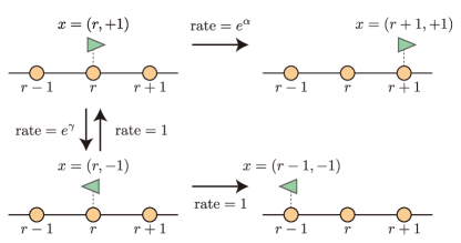
Figure 3: We consider a standard model of a discrete system with an odd degrees of freedom lee2013fluctuation ; spinney2012nonequilibrium ; ford2012entropy : a particle on a ring of $L$ states with position $r\in\{1,\dots,L\}$ and velocity $v\in\{-1,+1\}$, where the velocity is odd.

In Fig. 4, we visualize the time-dependent values of EPR $\dot{\sigma}$, our excess EPR $\dot{\sigma}_{\text{ex}}$, and the HS excess EPR $\dot{\sigma}_{\text{ex}}^{\text{HS}}$. We consider a system with $L=4$ positions and the non-stationary initial distribution $p_{rv}\propto 10\delta_{r0}\delta_{v1}+1$. We consider four conditions:

1. $\alpha=0$ and $\gamma=0$, so that all transitions are symmetric. Here the forces are conservative, $f={-\nabla}\bm{\phi}$ for $\phi_{x}=\ln p_{x}$ and the steady-state distribution is symmetric under conjugation of odd variables. The steady state is in equilibrium and $\dot{\sigma}=\dot{\sigma}_{\text{ex}}=\dot{\sigma}_{\text{ex}}^{\text{HS}}$ at all times.

2. $\alpha=0$ and $\gamma=1$, so velocity flips $(r,-1)\to(r,+1)$ occur more frequently than $(r,+1)\to(r,-1)$. The forces are conservative, $f={-\nabla}\bm{\phi}$ for $\phi_{x}=\ln p_{x}$, but the steady state is not symmetric under conjugation of odd variables. The steady state is not in equilibrium ($\dot{\sigma}>0$ in steady state). Since the forces are conservative, under our decomposition the housekeeping EPR vanishes and $\dot{\sigma}=\dot{\sigma}_{\text{ex}}$ at all times. The HS decomposition gives different results, which can take unphysical negative values: $\dot{\sigma}_{\text{ex}}^{\text{HS}}>\dot{\sigma},\dot{\sigma}_{\text{hk}}^{\text{HS}}<0$.

3. $\alpha=1$ and $\gamma=0$, so movements along the ring with positive velocity are faster than those with negative velocity. The steady state is symmetric under time-reversal but the forces $f_{(r,v)\to(r+v,v)}$ are not conservative, so the steady state is out of equilibrium. Our decomposition and HS decomposition both obey $0\leq\dot{\sigma}_{\text{ex}}\leq\dot{\sigma}$ and $0\leq\dot{\sigma}_{\text{ex}}^{\text{HS}}\leq\dot{\sigma}$. We also verify that, in systems with steady states that symmetric under time reversal, $\dot{\sigma}_{\text{ex}}\geq\dot{\sigma}_{\text{ex}}^{\text{HS}}$ always (Eq. S59 in Section SM7.1) and $\dot{\sigma}_{\text{ex}}=\dot{\sigma}_{\text{ex}}^{\text{HS}}=0$ in steady state.

4. $\alpha=1$ and $\gamma=1$, so the forces are not conservative and the steady state is not symmetric under conjugation of odd variables. The HS decomposition again gives unphysical values $\dot{\sigma}_{\text{ex}}^{\text{HS}}>\dot{\sigma},\dot{\sigma}_{\text{hk}}^{\text{HS}}<0$. Under our decomposition, neither $\dot{\sigma}_{\text{ex}}$ nor $\dot{\sigma}_{\text{hk}}$ vanish in steady state.

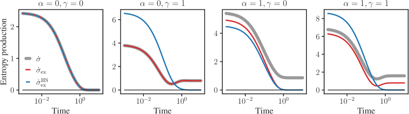
Figure 4: Plots of overall EPR $\dot{\sigma}$, our excess EPR $\dot{\sigma}_{\text{ex}}$, and the HS excess EPR $\dot{\sigma}_{\text{ex}}^{\text{HS}}$ for the ring model with an odd velocity variable. When $\alpha\neq 0$ the forces are non-conservative, when $\gamma\neq 0$ the steady-state distribution is not symmetric under conjugation of odd variables. The HS decomposition can give unphysical values ($\dot{\sigma}_{\text{ex}}^{\text{HS}}>\dot{\sigma},\dot{\sigma}_{\text{hk}}^{\text{HS}}<0$) when $\gamma\neq 0$.

Comparisons with other decompositions

SM7.1   Hatano-Sasa decomposition

Here we compare our information-geometric housekeeping/excess decomposition, $\dot{\sigma}=\dot{\sigma}_{\text{ex}}+\dot{\sigma}_{\text{hk}}$, to the HS housekeeping/excess decomposition, $\dot{\sigma}=\dot{\sigma}_{\text{hk}}^{\text{HS}}+\dot{\sigma}_{\text{ex}}^{\text{HS}}$. We derive the following inequality:

$$\dot{\sigma}_{\text{hk}}\leq\dot{\sigma}_{\text{hk}}^{\text{HS}}\qquad\dot{\sigma}_{\text{ex}}\geq\dot{\sigma}_{\text{ex}}^{\text{HS}}$$ (S59)

for (1) stochastic master equations without odd variables, (2) stochastic master equations with odd variables and time-symmetric steady states, and (3) chemical systems with complex balance and mass action kinetics. In all cases, we show that the HS housekeeping EPR can be written as the generalized KL divergence

$$\dot{\sigma}_{\text{hk}}^{\text{HS}}=\mathcal{D}(\bm{f}\|{-\nabla}\bm{\phi}^{\mathrm{ss}}),$$ (S60)

where $\phi_{x}^{\mathrm{ss}}:=\ln(p_{x}/\pi_{x})$ is defined via the steady-state distribution $\bm{\pi}$. Since our housekeeping EPR satisfies the variational principle in Eq. (4), Eq. S60 implies Eq. S59.

We first consider the simplest case, a stochastic master equation without odd variables. The EPR is given by (esposito2010threefaces, )

$$\dot{\sigma}=\sum_{y\neq x,\alpha}p_{x}R_{yx}^{\alpha}\ln\frac{p_{x}R_{yx}^{\alpha}}{p_{y}R_{xy}^{\alpha}},$$ (S61)

where $\alpha$ indexes over thermodynamic reservoirs. The HS excess and housekeeping terms are then given by (esposito2007entropy, ; esposito2010threefaces, )

$$\dot{\sigma}_{\text{ex}}^{\text{HS}} =\sum_{y\neq x,\alpha}p_{x}R_{yx}^{\alpha}\ln\frac{p_{x}\pi_{y}}{\pi_{x}p_{y}}$$ (S62)

$$\dot{\sigma}_{\text{hk}}^{\text{HS}} =\dot{\sigma}-\dot{\sigma}_{\text{ex}}^{\text{HS}}=\sum_{y\neq x,\alpha}p_{x}R_{yx}^{\alpha}\ln\frac{p_{x}R_{yx}^{\alpha}}{p_{x}R_{\epsilon x\epsilon y}^{\alpha}\pi_{y}/\pi_{x}}.$$ (S63)

Within our exponential family Eq. (1), the potential $\bm{\phi}^{\mathrm{ss}}$ gives rise to the fluxes

$$[\bm{j}({-\nabla}\bm{\phi}^{\mathrm{ss}})]_{x\to y;\alpha}=p_{y}R_{\epsilon x\epsilon y}^{\alpha}e^{\ln p_{x}/\pi_{x}-\ln p_{y}/\pi_{y}}=p_{x}R_{\epsilon x\epsilon y}^{\alpha}\pi_{y}/\pi_{x}.$$

It leads to the following generalized KL divergence,

$$\mathcal{D}(\bm{f}\|{-\nabla}\bm{\phi}^{\mathrm{ss}})= \sum_{y\neq x,\alpha}p_{x}R_{yx}^{\alpha}\ln\frac{p_{x}R_{yx}^{\alpha}}{p_{x}R_{\epsilon x\epsilon y}^{\alpha}\pi_{y}/\pi_{x}}-p_{x}R_{yx}^{\alpha}+p_{x}R_{\epsilon x\epsilon y}^{\alpha}\frac{\pi_{y}}{\pi_{x}}$$ (S64)

$$= \sum_{y\neq x,\alpha}p_{x}R_{yx}^{\alpha}\ln\frac{p_{x}R_{yx}^{\alpha}}{p_{x}R_{\epsilon x\epsilon y}^{\alpha}\pi_{y}/\pi_{x}}=\dot{\sigma}_{\text{hk}}^{\text{HS}},$$ (S65)

where in the second line we used that

$$\sum_{y\neq x,\alpha}\left(p_{x}R_{\epsilon x\epsilon y}^{\alpha}\frac{\pi_{y}}{\pi_{x}}-p_{x}R_{yx}^{\alpha}\right) =\sum_{x}\frac{p_{x}}{\pi_{x}}\sum_{y(\neq x),\alpha}\left(\pi_{y}R_{\epsilon x\epsilon y}^{\alpha}-\pi_{x}R_{yx}^{\alpha}\right)=0,$$

which follows since $\bm{\pi}$ is a steady-state distribution. In this way, we derived Eq. S60 in Eq. S65.

Next, we consider stochastic master equations with odd variables, under the assumption that the steady-state distribution is symmetric under conjugation of odd variables $\pi_{x}=\pi_{\epsilon x}$. As shown in Eq. S56 in Section SM6, the EPR is

$$\dot{\sigma}=\sum_{y\neq x,\alpha}\big{(}p_{x}R_{yx}^{\alpha}\ln\frac{p_{x}R_{yx}^{\alpha}}{p_{y}R_{\epsilon x\epsilon y}^{\alpha}}-p_{x}R_{yx}^{\alpha}+p_{y}R_{\epsilon x\epsilon y}^{\alpha}\big{)}.$$ (S66)

The HS excess EPR is still defined as in Eq. S62, while the HS housekeeping EPR is the remainder (spinney2012nonequilibrium, ; lee2013fluctuation, ):

$$\dot{\sigma}_{\text{hk}}^{\text{HS}} =\dot{\sigma}-\dot{\sigma}_{\text{ex}}^{\text{HS}}=\sum_{y\neq x,\alpha}\big{(}p_{x}R_{yx}^{\alpha}\ln\frac{p_{x}R_{yx}^{\alpha}}{p_{x}R_{\epsilon x\epsilon y}^{\alpha}\pi_{y}/\pi_{x}}-p_{x}R_{yx}^{\alpha}+p_{y}R_{\epsilon x\epsilon y}^{\alpha}\big{)}.$$ (S67)

The potential $\bm{\phi}^{\mathrm{ss}}$ gives rise to the fluxes

$$[\bm{j}({-\nabla}\bm{\phi}^{\mathrm{ss}})]_{x\to y;\alpha}=p_{y}R_{\epsilon x\epsilon y}^{\alpha}e^{\ln p_{x}/\pi_{x}-\ln p_{y}/\pi_{y}}=p_{x}R_{\epsilon x\epsilon y}^{\alpha}\frac{\pi_{y}}{\pi_{x}},$$

and leads to the following generalized KL divergence

$$\mathcal{D}(\bm{f}\|{-\nabla}\bm{\phi}^{\mathrm{ss}})= \sum_{y\neq x,\alpha}p_{x}R_{yx}^{\alpha}\ln\frac{p_{x}R_{yx}^{\alpha}}{p_{x}R_{\epsilon x\epsilon y}^{\alpha}\frac{\pi_{y}}{\pi_{x}}}-p_{x}R_{yx}^{\alpha}+p_{x}R_{\epsilon x\epsilon y}^{\alpha}\frac{\pi_{y}}{\pi_{x}}.$$

Finally, we have

$$\sum_{y\neq x,\alpha}\Big{(}p_{x}R_{\epsilon x\epsilon y}^{\alpha}\pi_{y}/\pi_{x}-p_{y}R_{\epsilon x\epsilon y}^{\alpha}\Big{)} =\sum_{y\neq x,\alpha}\Big{(}p_{x}R_{\epsilon x\epsilon y}^{\alpha}\pi_{y}/\pi_{x}-p_{x}R_{\epsilon y\epsilon x}^{\alpha}\Big{)}$$

$$=\sum_{x}\frac{p_{x}}{\pi_{x}}\sum_{y(\neq x),\alpha}\Big{(}R_{\epsilon x\epsilon y}^{\alpha}\pi_{y}-R_{\epsilon x\epsilon y}^{\alpha}\pi_{x}\Big{)}$$

$$=\sum_{x}\frac{p_{x}}{\pi_{x}}\sum_{y(\neq x),\alpha}\Big{(}R_{\epsilon x\epsilon y}^{\alpha}\pi_{\epsilon y}-R_{\epsilon x\epsilon y}^{\alpha}\pi_{\epsilon x}\Big{)}=0,$$

where we used the symmetry $\pi_{x}=\pi_{\epsilon x}$. Plugging $\sum_{y\neq x,\alpha}p_{x}R_{\epsilon x\epsilon y}^{\alpha}\frac{\pi_{y}}{\pi_{x}}=\sum_{y\neq x,\alpha}p_{y}R_{\epsilon x\epsilon y}^{\alpha}$ into Eq. S67 implies Eq. S60.

Finally, we consider chemical systems that obey complex balance, meaning that the net current entering and leaving each chemical complex vanishes in steady state (feinbergFoundationsChemicalReaction2019, ). We also assume mass action kinetics, as in Eq. S14. In that case, the HS excess and housekeeping EPR is (ge2016nonequilibrium, ; rao2016nonequilibrium, )

$$\dot{\sigma}_{\text{ex}}^{\text{HS}} =-\sum_{\rho}J_{\rho}\sum_{x}\nabla_{\rho x}\ln\frac{c_{x}}{\pi_{x}}.$$ (S68)

$$\dot{\sigma}_{\text{hk}}^{\text{HS}} =\dot{\sigma}-\dot{\sigma}_{\text{ex}}^{\text{HS}}=\sum_{\rho}J_{\rho}\left[\ln\frac{J_{\rho}}{J_{\tilde{\rho}}}+\sum_{x}\nabla_{\rho x}\ln\frac{c_{x}}{\pi_{x}}\right],$$ (S69)

where $\bm{c}$ is the vector actual concentrations and $\bm{\pi}$ is the vector of steady-state concentrations ($\bm{c}$ and $\bm{\pi}$ are nonnegative, but do not necessarily sum to 1). Using the potential $\phi_{x}^{\text{ss}}:=\ln(c_{x}/\pi_{x})$, Eq. S69 can be written as

$$\dot{\sigma}_{\text{hk}}^{\text{HS}}=\bm{J}^{T}(\bm{f}+\nabla\bm{\phi}^{\mathrm{ss}}).$$

Using this expression and Eq. (2), we write

$$\mathcal{D}(\bm{f}\|{-\nabla}\bm{\phi}^{\mathrm{ss}})=\dot{\sigma}_{\text{hk}}^{\text{HS}}-V,$$ (S70)

where for notational convenience we defined

$$V=\sum_{\rho}(J_{\rho}-J_{\tilde{\rho}}e^{[{-\nabla}\bm{\phi}^{\mathrm{ss}}]_{\rho}}).$$ (S71)

We prove Eq. S60 by showing that $V=0$.

To begin, split the right hand side of Eq. S71 into contributions from the forward and negative side of each reversible reaction $r$ (see discussion of notation in Section SM1),

$$V=\sum_{r}(J_{r}^{\rightarrow}-J_{r}^{\leftarrow}e^{[{-\nabla}\bm{\phi}^{\mathrm{ss}}]_{r}})+\sum_{r}(J_{r}^{\rightarrow}-J_{r}^{\leftarrow}e^{[{\nabla}\bm{\phi}^{\mathrm{ss}}]_{r}}).$$ (S72)

Using Eq. S14, each term in the first sum can be written as

$$J_{r}^{\rightarrow}-J_{r}^{\leftarrow}e^{[{-\nabla}\bm{\phi}^{\mathrm{ss}}]_{r}} =k_{r}^{\rightarrow}\prod_{x}c_{x}^{\nu_{xr}}-k_{r}^{\leftarrow}\prod_{x}c_{x}^{\kappa_{xr}}\prod_{x}\Big{(}\frac{c_{x}}{\pi_{x}}\Big{)}^{\nu_{xr}-\kappa_{xr}}$$

$$=\prod_{x}\Big{(}\frac{c_{x}}{\pi_{x}}\Big{)}^{\nu_{xr}}\left(k_{r}^{\rightarrow}\prod_{x}\pi_{x}^{\nu_{xr}}-k_{r}^{\leftarrow}\prod_{x}\pi_{x}^{\kappa_{xr}}\right)=\prod_{x}\Big{(}\frac{c_{x}}{\pi_{x}}\Big{)}^{\nu_{xr}}\mathcal{J}_{\rho}^{\mathrm{ss}},$$

where $\mathcal{J}_{\rho}^{\mathrm{ss}}$ is the current (net flux) across reversible reaction $r$ in steady state. Using a similar derivation, we write each term in the second sum in Eq. S72 as

$$J_{r}^{\rightarrow}-J_{r}^{\leftarrow}e^{[\nabla\bm{\phi}^{\mathrm{ss}}]_{r}}=-\prod_{x}\Big{(}\frac{c_{x}}{\pi_{x}}\Big{)}^{\kappa_{xr}}\mathcal{J}_{\rho}^{\mathrm{ss}}.$$ (S73)

Combining, we rewrite Eq. S71 as

$$V=\sum_{r}\left[\prod_{x}\Big{(}\frac{c_{x}}{\pi_{x}}\Big{)}^{\nu_{xr}}\mathcal{J}_{\rho}^{\mathrm{ss}}-\prod_{x}\Big{(}\frac{c_{x}}{\pi_{x}}\Big{)}^{\kappa_{xr}}\mathcal{J}_{\rho}^{\mathrm{ss}}\right].$$ (S74)

Now split the right hand side into contributions from each reactant complex and each product complex. Let $C$ indicate the set of reactant and product complexes, where each element of $C$ is a vector $\bm{\eta}\in\mathbb{\mathbb{N}}_{0}^{N}$ with ${\eta}_{x}$ is the number of species $x$ in complex $\bm{\eta}$. Let $A(\bm{\eta})=\{r:\nu_{xr}={\eta}_{x}\forall x\}$ indicate the set of reactions that have reactant complex $\bm{\eta}$, and let $B(\bm{\eta})=\{r:\kappa_{xr}={\eta}_{x}\forall x\}$ indicate the set of reactions that have product complex $\bm{\eta}$. Then, we can rewrite Eq. S74

$$V =\sum_{\bm{\eta}\in C}\left[\sum_{r\in A(\bm{\eta})}\prod_{x}\Big{(}\frac{c_{x}}{\pi_{x}}\Big{)}^{\nu_{xr}}\mathcal{J}_{\rho}^{\mathrm{ss}}-\sum_{r\in B(\bm{\eta})}\prod_{x}\Big{(}\frac{c_{x}}{\pi_{x}}\Big{)}^{\kappa_{xr}}\mathcal{J}_{\rho}^{\mathrm{ss}}\right]$$

$$=\sum_{\bm{\eta}\in C}\left[\sum_{r\in A(\bm{\eta})}\prod_{x}\Big{(}\frac{c_{x}}{\pi_{x}}\Big{)}^{{\eta}_{x}}\mathcal{J}_{\rho}^{\mathrm{ss}}-\sum_{r\in B(\bm{\eta})}\prod_{x}\Big{(}\frac{c_{x}}{\pi_{x}}\Big{)}^{{\eta}_{x}}\mathcal{J}_{\rho}^{\mathrm{ss}}\right]$$

$$=\sum_{\bm{\eta}\in C}\prod_{x}\Big{(}\frac{c_{x}}{\pi_{x}}\Big{)}^{{\eta}_{x}}\left[\sum_{r\in A(\bm{\eta})}\mathcal{J}_{\rho}^{\mathrm{ss}}-\sum_{r\in B(\bm{\eta})}\mathcal{J}_{\rho}^{\mathrm{ss}}\right].$$

By the definition of complex balance, $\sum_{r\in A(\bm{\eta})}\mathcal{J}_{\rho}^{\mathrm{ss}}=\sum_{r\in B(\bm{\eta})}\mathcal{J}_{\rho}^{\mathrm{ss}}$ for each $\bm{\eta}$  (feinbergFoundationsChemicalReaction2019, ). Therefore, $V=0$, which implies Eq. S60.

SM7.2   “Onsager-projective decomposition” from Ref. (kohei2022, )

This paper builds on recent work by the present authors (kohei2022, ), which studied excess and housekeeping EPR in discrete Markovian systems. It considered both on linear stochastic master equations and nonlinear chemical reaction networks, though only without odd variables (see also Refs. (dechant2022geometric, ; dechant2022geometricCoupling, ) for continuous systems).

As in the present paper, Ref. (kohei2022, ) considers the excess and housekeeping decomposition from a geometric perspective. In that paper, the EPR is written as the squared (generalized) Euclidean norm of the force vector under an appropriate metric:

$$\dot{\sigma}=\left\|\bm{f}\right\|_{L}^{2}\equiv\bm{f}^{T}L\bm{f},$$ (S75)

where $\bm{f}\in\mathbb{R}^{M}$ is the thermodynamic force (same as in this paper) and $L$ is a diagonal matrix $\mathbb{R}_{+}^{M\times M}$ of edgewise Onsager coefficients,

$$L_{\rho\rho}=\frac{1}{2}(J_{\rho}-J_{\tilde{\rho}})/f_{\rho}.$$ (S76)

(The factor 1/2 appears here but not in Ref. (kohei2022, ) due to a minor change of convention: unlike Ref. (kohei2022, ), in this paper we consider reversible reactions as two separate reactions.) The force vector is projected onto the subspace of conservative forces, which gives rise to the optimal potential:

$$\bm{\phi}_{\text{ons}}^{*}=\operatorname*{\arg\,\min}_{\bm{\phi}\in\mathbb{R}^{M}}\big{\|}\bm{f}-({-\nabla}\bm{\phi})\big{\|}_{L}^{2}.$$ (S77)

where the subscript “ons” refers to the Onsager metric. The housekeeping EPR is then defined as the squared (generalized) Euclidean distance from $\bm{f}$ to the subspace of conservative forces, while the excess EPR is defined as the squared (generalized) Euclidean norm of the projected conservative force,

$$\dot{\sigma}=\left\|\bm{f}\right\|_{L}^{2}=\underbrace{\left\|\bm{f}-({-\nabla}\bm{\phi}_{\text{ons}}^{*})\right\|_{L}^{2}}_{\dot{\sigma}_{\text{hk}}^{\text{ons}}}+\underbrace{\left\|\nabla\bm{\phi}_{\text{ons}}^{*}\right\|_{L}^{2}}_{\dot{\sigma}_{\text{ex}}^{\text{ons}}}.$$ (S78)

We refer to $\dot{\sigma}_{\text{hk}}^{\text{ons}}$ and $\dot{\sigma}_{\text{ex}}^{\text{ons}}$ as the Onsager-projective housekeeping and excess EPR terms.

In this paper, we work within the non-Euclidean setting of information geometry. In our case, distance is measured in terms of KL divergence rather than generalized Euclidean norm. Nonetheless, it is clear that Eq. (4) is the information-geometric analogue of Eq. S77, while Eq. (6) is the information-geometric analogue of Eq. S78. Thus, our approach is an information-geometric extension of Ref. (kohei2022, ).

Euclidean geometry suffices for systems that exhibit Onsager-type linear relations between thermodynamic forces and fluxes, as occurs near steady state or near equilibrium. On the other hand, far-from-equilibrium analysis requires an information-geometric treatment. For this reason, the TURs and TSLs derived in Ref. (kohei2022, ) are in general only tight for systems that are close to equilibrium and/or steady state, while the bounds derived in this paper can be tight arbitrarily far from equilibrium.

However, we can relate the two decompositions. In accordance with Ref. (kohei2022, ), we restrict our attention to systems without odd variables, and show that

$$\dot{\sigma}_{\text{hk}}\geq\dot{\sigma}_{\text{hk}}^{\text{ons}}\qquad\dot{\sigma}_{\text{ex}}\leq\dot{\sigma}_{\text{ex}}^{\text{ons}}.$$ (S79)

To derive this result, recall that for systems without odd variables, each reaction $\rho$ is paired with a unique reverse reaction $\tilde{\rho}$ such that $f_{\tilde{\rho}}=-f_{\rho}$. Consider the KL divergence between the forward fluxes $\bm{J}=\bm{j}(\bm{f})$ and any other $\bm{j}(\bm{\theta})$ where $\bm{\theta}$ is anti-symmetric ($\theta_{\rho}=-\theta_{\tilde{\rho}}$):

$$\mathcal{D}(\bm{f}\|\bm{\theta}) =\sum_{\rho}J_{\rho}(e^{-(f_{\rho}-\theta_{\rho})}+(f_{\rho}-\theta_{\rho})-1)$$

$$=\sum_{\rho}J_{\tilde{\rho}}(e^{f_{\rho}-\theta_{\rho}}-(f_{\rho}-\theta_{\rho})-1).$$

On the first line we rearranged Eq. (2) in the main text, and in the second line we used anti-symmetry of $\bm{f}$ and $\bm{\theta}$. Combining these expressions, and using $J_{\rho}=e^{f_{\rho}}J_{\tilde{\rho}}$, gives

$$\mathcal{D}(\bm{f}\|\bm{\theta})=\frac{1}{2}\sum_{\rho}J_{\tilde{\rho}}\big{(}(e^{f_{\rho}-\theta_{\rho}}-(f_{\rho}-\theta_{\rho})-1)+e^{f_{\rho}}(e^{-(f_{\rho}-\theta_{\rho})}+(f_{\rho}-\theta_{\rho})-1)\big{)}.$$

We now rewrite the right hand side as

$$\mathcal{D}(\bm{f}\|\bm{\theta}) =\frac{1}{2}\sum_{\rho}J_{\tilde{\rho}}\big{(}h(f_{\rho}-\theta_{\rho},f_{\rho})+\frac{e^{f}-1}{f}(f_{\rho}-\theta_{\rho})^{2}\big{)}$$

$$=\frac{1}{2}\sum_{\rho}J_{\tilde{\rho}}h(f_{\rho}-\theta_{\rho},f_{\rho})+\left\|\bm{f}-\bm{\theta}\right\|_{L}^{2},\!\!\!\!\!\!$$ (S80)

where for convenience we defined the following function:

$$h(a,b)=\Big{[}\frac{(e^{a}-a-1)+e^{b}(e^{-a}+a-1)}{a^{2}}-\frac{e^{b}-1}{b}\Big{]}a^{2}.$$

It can be verified (e.g., by taking derivatives with respect to $a$) that the term inside the brackets is nonnegative. Thus, $h$ is nonnegative, therefore $\mathcal{D}(\bm{f}\|\bm{\theta})\geq\left\|\bm{f}-\bm{\theta}\right\|_{L}^{2}$ given Eq. S80. Finally, since $\bm{\theta}={-\nabla}\bm{\phi}$ is anti-symmetric, we arrive at Eq. S79:

$$\dot{\sigma}_{\text{hk}}=\min_{\bm{\phi}}\mathcal{D}(\bm{f}\|{-\nabla}\bm{\phi})\geq\min_{\bm{\phi}}\left\|\bm{f}-({-\nabla}\bm{\phi})\right\|_{L}^{2}=\dot{\sigma}_{\text{hk}}^{\text{ons}}.$$

For a numerical comparison between the decomposition proposed in this paper and Ref. (kohei2022, ), see Section SM7.3.

We now consider the limit in which the two decompositions agree. Using the derivations above, we have the bounds

$$0\leq\dot{\sigma}_{\text{hk}}-\dot{\sigma}_{\text{hk}}^{\text{ons}}\leq\frac{1}{2}\sum_{\rho}J_{\tilde{\rho}}\,h(f_{\rho}+[\nabla\bm{\phi}_{\text{ons}}^{*}]_{\rho},f_{\rho}).$$ (S81)

The function $h(a,b)$ vanishes to first order around $a=b$ and $a=0$ (in general, $h(a,b)$ is symmetric under the transformation $a\mapsto b-a$). In the context of Eq. S81, $a=b$ reflects that $\dot{\sigma}_{\text{hk}}$ and $\dot{\sigma}_{\text{hk}}^{\text{ons}}$ agree to first order around $\nabla\bm{\phi}_{\text{ons}}^{*}=0$ (steady state) while $a=0$ reflects that they agree to first order around $\bm{f}={-\nabla}\bm{\phi}_{\text{ons}}^{*}$ (the forces are conservative). We can ask if they also agree to second order there. A Taylor expansion of $h(a,b)$ shows that second order terms do not vanish except in the limit $b\to 0$. In the context of Eq. S81, this is the equilibrium limit $f_{\rho}\to 0$, where the thermodynamic force across each reaction vanishes. Note that

$$c_{1}\left\|\bm{f}\right\|^{2}\geq\left\|\bm{f}\right\|_{L}^{2}\geq\left\|\bm{f}+\nabla\bm{\phi}_{\text{ons}}^{*}\right\|_{L}^{2}\geq c_{2}\left\|\bm{f}+\nabla\bm{\phi}_{\text{ons}}^{*}\right\|^{2}$$

where $c_{1}=\max(J_{\rho}+J_{\tilde{\rho}})/2$, $c_{2}=\min_{\rho}\sqrt{J_{\rho}J_{\tilde{\rho}}}$, and $\|\cdot\|$ is the usual Euclidean norm (we used Eq. S78 for the middle inequality, the others come from bounds on the logarithmic mean in Eq. S76). Thus, if $f_{\rho}\to 0$, we can assume that $f_{\rho}+[\nabla\bm{\phi}_{\text{ons}}^{*}]_{\rho}$, first argument of $h$, also vanishes in Eq. S81. We now expand $h$ in each argument and rearrange to give

$$h(\gamma,f)=\frac{1}{12}\gamma^{2}\left(\gamma-f\right)^{2}+\mathcal{O}(\epsilon^{5})=\mathcal{O}(\epsilon^{4})$$ (S82)

for $f,\gamma\sim\epsilon$. Plugging into Eq. S81 shows that $\dot{\sigma}_{\text{hk}}$ and $\dot{\sigma}_{\text{hk}}^{\text{ons}}$ agree to third order in the equilibrium limit.

As discussed in Ref. (kohei2022, ), the Onsager-projective decomposition can be seen as an extension of the Maes and Netočný (MN) approach (maes2014nonequilibrium, ) to discrete systems. The decomposition proposed in this paper can be seen as a generalization of the MN decomposition to the far-from-equilibrium regime.

SM7.3   Numerical comparison with Refs. (kohei2022, ) and (Kobayashi2022, )

Here, we numerically compare three decompositions: the Onsager-projective decomposition described in Section SM7.2, the “Hessian decomposition” which was recently proposed in Ref. (Kobayashi2022, ), and the information-geometric decomposition that we propose in this Letter. While an inequality exists between the Onsager decomposition and our decomposition, Eq. S79, no inequality between the Hessian decomposition and the others has been proved analytically. Nonetheless, our numerical results prove that they are different. They also suggest that the Hessian decomposition gives intermediate values between the other two decompositions.

To be self-contained, we briefly review the Hessian decomposition presented in Ref. (Kobayashi2022, ). Consider a system without odd variables that has $M$ reactions, having forward and reverse fluxes $J_{\rho}$ and $J_{\tilde{\rho}}$. We adopt the notation defined in Section SM1: we use $r\in\{1,2,\dots,M/2\}$ to label each pair of reactions $\rho$ and $\tilde{\rho}$, where the forward/reverse fluxes of the pair are indicated as $J_{r}^{\rightarrow}=J_{\rho}$ and $J_{r}^{\leftarrow}=J_{\tilde{\rho}}$. We define a vector of currents (net fluxes) $\bm{\mathcal{J}}\in\mathbb{R}^{M/2}$ as $\mathcal{J}_{r}:=J_{r}^{\rightarrow}-J_{r}^{\leftarrow}$, a vector of “frenetic activities” $\bm{\omega}\in\mathbb{R}_{+}^{M/2}$ as $\omega_{r}:=2\sqrt{J_{r}^{\rightarrow}J_{r}^{\leftarrow}}$, and a vector of (half)forces $\bm{\mathcal{F}}\in\mathbb{R}^{M/2}$ as $\mathcal{F}_{r}=\frac{1}{2}\ln(J_{r}^{\rightarrow}/J_{r}^{\leftarrow})$. We use the notation $\bar{\nabla}^{T}$ to indicate the $N\times M/2$ matrix that only has columns for the forward reaction ($\rho$) in each pair $(\rho,\tilde{\rho})$. $\bar{\nabla}^{T}$ maps currents to time evolution vectors: $\mathrm{d}_{t}\bm{p}=\bar{\nabla}^{T}\bm{\mathcal{J}}=\nabla^{T}\bm{J}$. We emphasize that Ref. (Kobayashi2022, ) uses the convention that forces $\mathcal{F}_{r}=\frac{1}{2}\ln(J_{r}^{\rightarrow}/J_{r}^{\leftarrow})$ are scaled by $1/2$ relative to the forces as defined in this paper, $f_{r}=\ln(J_{r}^{\rightarrow}/J_{r}^{\leftarrow})$.

Observe that the currents can be expressed as

$$\mathcal{J}_{r}=\omega_{r}\sinh(\mathcal{F}_{r})=\sqrt{J_{r}^{\rightarrow}J_{r}^{\leftarrow}}\left(\sqrt{\frac{J_{r}^{\rightarrow}}{J_{r}^{\leftarrow}}}-\sqrt{\frac{J_{r}^{\leftarrow}}{J_{r}^{\rightarrow}}}\right)=J_{r}^{\rightarrow}-J_{r}^{\leftarrow}.$$

Conversely, this equation can be solved for $\mathcal{F}_{r}$ as

$$\mathcal{F}_{r}=\sinh^{-1}(\mathcal{J}_{r}/\omega_{r}).$$

These relations can also be derived from a higher level structure. Define two dual convex functions which are the Legendre conjugate of each other: for a fixed $\bm{\omega}$, the convex function

$$\Psi_{\omega}(\bm{\mathcal{J}}^{\prime}):=\sum_{r}\left[\mathcal{J}_{r}^{\prime}\sinh^{-1}(\mathcal{J}_{r}^{\prime}/\omega_{r})-\omega_{r}\left[\sqrt{1+(\mathcal{J}_{r}^{\prime}/\omega_{r})^{2}}-1\right]\right]$$

is the Legendre conjugate of

$$\Psi_{\omega}^{*}(\bm{\mathcal{F}}^{\prime})=\sum_{r}\omega_{r}\Big{[}\cosh(\mathcal{F}_{r}^{\prime})-1\Big{]},$$

and they specify the current and force across reaction $r$ as

$$\mathcal{J}_{r}=\partial_{\mathcal{F}_{r}}\Psi_{\omega}^{*}(\bm{\mathcal{F}}),\quad\mathcal{F}_{r}=\partial_{\mathcal{J}_{r}}\Psi_{\omega}(\bm{\mathcal{J}}).$$

Note that for any $\bm{\omega}$, $\Psi_{\omega}(\bm{0})=\Psi_{\omega}^{*}(\bm{0})=0$ holds and it is their minima. In general, a convex function $\varphi(\bm{x})$ leads to the Bregman divergence $D(\bm{x}\|\bm{x}^{\prime}):=\varphi(\bm{x})-\varphi(\bm{x}^{\prime})-\langle\bm{x}-\bm{x}^{\prime},\nabla\varphi(\bm{x}^{\prime})\rangle\geq 0$, where $\langle\cdot,\cdot\rangle$ is the normal inner product and $\nabla\varphi(\bm{x})$ is the gradient vector $(\partial_{x_{1}}\varphi(\bm{x}),\partial_{x_{2}}\varphi(\bm{x}),\dots)^{T}$ of the function (amari2016information, ). For a fixed $\bm{\omega}$, we can define the Bregman divergences $D_{\omega}$ and the dual one $D_{\omega}^{*}$ by

$$D_{\omega}(\bm{\mathcal{J}}^{\prime}\|\bm{\mathcal{J}}^{\prime\prime}) \!:=\!\Psi_{\omega}(\bm{\mathcal{J}}^{\prime})\!-\!\Psi_{\omega}(\bm{\mathcal{J}}^{\prime\prime})\!-\!\langle\bm{\mathcal{J}}^{\prime}\!-\!\bm{\mathcal{J}}^{\prime\prime},\nabla\Psi_{\omega}(\bm{\mathcal{J}}^{\prime\prime})\rangle$$

$$D_{\omega}^{*}(\bm{\mathcal{F}}^{\prime}\|\bm{\mathcal{F}}^{\prime\prime}) \!:=\!\Psi_{\omega}^{*}(\bm{\mathcal{F}}^{\prime})\!-\!\Psi_{\omega}^{*}(\bm{\mathcal{F}}^{\prime\prime})\!-\!\langle\bm{\mathcal{F}}^{\prime}\!-\!\bm{\mathcal{F}}^{\prime\prime},\nabla\Psi_{\omega}^{*}(\bm{\mathcal{F}}^{\prime\prime})\rangle$$

As a general property of Bregman divergences and the Legendre transformation, we have

$$D_{\omega}(\bm{\mathcal{J}}^{\prime}\|\bm{\mathcal{J}}^{\prime\prime})=D_{\omega}^{*}(\bm{\mathcal{F}}^{\prime\prime}\|\bm{\mathcal{F}}^{\prime})$$ (S83)

when $(\bm{\mathcal{J}}^{\prime},\bm{\mathcal{F}}^{\prime})$ and $(\bm{\mathcal{J}}^{\prime\prime},\bm{\mathcal{F}}^{\prime\prime})$ are Legendre dual coordinates. In this situation, we also have

$$D_{\omega}(\bm{\mathcal{J}}^{\prime}\|\bm{\mathcal{J}}^{\prime\prime})=\Psi_{\omega}(\bm{\mathcal{J}}^{\prime})+\Psi_{\omega}^{*}(\bm{\mathcal{F}}^{\prime\prime})-\langle\bm{\mathcal{J}}^{\prime},\bm{\mathcal{F}}^{\prime\prime}\rangle,$$ (S84)

which leads to

$$\dot{\sigma}=\langle\bm{\mathcal{J}},\bm{\mathcal{F}}\rangle=\Psi_{\omega}(\bm{\mathcal{J}})+\Psi_{\omega}^{*}(\bm{\mathcal{F}}).$$ (S85)

Note that in general, these Bregman divergences cannot be expressed as KL divergence because the current $\mathcal{J}_{r}$ can be negative. Therefore, they cannot be related to the EPR, in the same way that we relate nonnegative one-way fluxes to EPR via the divergence $\mathcal{D}$ in Eq. (3).

The Hessian decomposition (Kobayashi2022, ) is defined by using two special points: $(\bm{\mathcal{J}}_{\mathrm{eq}},\bm{\mathcal{F}}_{\mathrm{eq}})$, which represent conservative currents/forces, and $(\bm{\mathcal{J}}_{\mathrm{ss}},\bm{\mathcal{F}}_{\mathrm{ss}})$, which represent steady-state currents/forces. Given these two pairs of currents/forces, we have

$$\dot{\sigma}_{\text{hk}}^{\text{hess}}:=\Psi_{\omega}(\bm{\mathcal{J}}_{\mathrm{eq}})+D_{\omega}^{*}(\bm{\mathcal{F}}\|\bm{\mathcal{F}}_{\mathrm{ss}}),$$ (S86)

$$\dot{\sigma}_{\text{ex}}^{\text{hess}}:=\Psi_{\omega}^{*}(\bm{f}_{\mathrm{ss}})+D_{\omega}(\bm{\mathcal{J}}\|\bm{\mathcal{J}}_{\mathrm{eq}}).$$ (S87)

To explain how $(\bm{\mathcal{J}}_{\mathrm{eq}},\bm{\mathcal{F}}_{\mathrm{eq}})$ and $(\bm{\mathcal{J}}_{\mathrm{ss}},\bm{\mathcal{F}}_{\mathrm{ss}})$ are determined, we define two kinds of sets. We define $\mathcal{P}(\bm{\mathcal{J}}^{\prime})$ as the set of currents that induce the same dynamics as $\bm{\mathcal{J}}^{\prime}$ by

$$\mathcal{P}(\bm{\mathcal{J}}^{\prime}):=\{\bm{\mathcal{J}}^{\prime\prime}\in\mathbb{R}^{M/2}\mid\bar{\nabla}^{T}\bm{\mathcal{J}}^{\prime\prime}=\bar{\nabla}^{T}\bm{\mathcal{J}}^{\prime}\}.$$ (S88)

The other space $\mathcal{M}_{\omega}(\bm{\mathcal{F}}^{\prime})$ is defined as the set of currents that are given by $\bm{\mathcal{F}}^{\prime}$ plus some conservative forces:

$$\mathcal{M}_{\omega}(\bm{\mathcal{F}}^{\prime}):=\{\nabla\Psi_{\omega}^{*}(\bm{\mathcal{F}}^{\prime\prime})\mid\bm{\mathcal{F}}^{\prime\prime}\in\bm{\mathcal{F}}^{\prime}+\mathrm{im}\,\bar{\nabla}\},$$ (S89)

where $\bm{\mathcal{F}}^{\prime}+\mathrm{im}\,\bar{\nabla}:=\{\bm{\mathcal{F}}^{\prime}+\bar{\nabla}\bm{\phi}\mid\bm{\phi}\in\mathbb{R}^{N}\}$. Then, $\bm{\mathcal{J}}_{\mathrm{eq}}$ and $\bm{\mathcal{J}}_{\mathrm{ss}}$ are given as unique intersections as

$$\bm{\mathcal{J}}_{\mathrm{eq}}:=\mathcal{P}(\bm{\mathcal{J}})\cap\mathcal{M}_{\omega}(\bm{0}),\;\;\bm{\mathcal{J}}_{\mathrm{ss}}:=\mathcal{P}(\bm{0})\cap\mathcal{M}_{\omega}(\bm{\mathcal{F}}),$$ (S90)

while the corresponding forces $\bm{\mathcal{F}}_{\mathrm{eq}}$ and $\bm{\mathcal{F}}_{\mathrm{ss}}$ are provided as $\nabla\Psi_{\omega}(\bm{\mathcal{J}}_{\mathrm{eq}})$ and $\nabla\Psi_{\omega}(\bm{\mathcal{J}}_{\mathrm{ss}})$. Therefore, we see that, with frenetic activity being fixed, $\bm{\mathcal{J}}_{\mathrm{eq}}$ is the current induced by a conservative force which recovers the original dynamics, while $\bm{\mathcal{J}}_{\mathrm{ss}}$ is the steady-state current which is given by a force that has the same nonconservative contribution as the actual force.

We note variational characterizations of $(\bm{\mathcal{J}}_{\mathrm{eq}},\bm{\mathcal{F}}_{\mathrm{eq}})$ and $(\bm{\mathcal{J}}_{\mathrm{ss}},\bm{\mathcal{F}}_{\mathrm{ss}})$, which can make easier to calculate the decomposition numerically. $\bm{\mathcal{J}}_{\mathrm{eq}}$ is given by

$$\bm{\mathcal{J}}_{\mathrm{eq}}=\operatorname*{\arg\,\min}_{\bm{\mathcal{J}}^{\prime}\in\mathcal{P}(\bm{\mathcal{J}})}\Psi_{\omega}(\bm{\mathcal{J}}^{\prime}),$$ (S91)

while $\bm{\mathcal{F}}_{\mathrm{ss}}$ is obtained as

$$\bm{\mathcal{F}}_{\mathrm{ss}}=\operatorname*{\arg\,\min}_{\bm{\mathcal{F}}^{\prime}\in\bm{\mathcal{F}}+\mathrm{im}\,\bar{\nabla}}\Psi_{\omega}^{*}(\bm{\mathcal{F}}^{\prime}).$$ (S92)

Next, let us focus on a specific chemical reaction network. In Ref. (Kobayashi2022, ), the authors discuss the reaction network

$$2X\underset{k_{1}^{\leftarrow}}{\overset{k_{1}^{\rightarrow}}{\rightleftarrows}}2Y\underset{k_{2}^{\leftarrow}}{\overset{k_{2}^{\rightarrow}}{\rightleftarrows}}X+Y\underset{k_{3}^{\leftarrow}}{\overset{k_{3}^{\rightarrow}}{\rightleftarrows}}2X,$$ (S93)

assuming the mass action kinetics with rate constants presented in the chemical equations. We calculate our EPRs $\dot{\sigma}_{\text{hk}}$, $\dot{\sigma}_{\text{ex}}$, the Onsager EPRs $\dot{\sigma}_{\text{hk}}^{\text{ons}}$, $\dot{\sigma}_{\text{ex}}^{\text{ons}}$, and the Hessian EPRs $\dot{\sigma}_{\text{hk}}^{\text{hess}}$, $\dot{\sigma}_{\text{ex}}^{\text{hess}}$, with the same parameters as Ref. (Kobayashi2022, ). Concretely, we used the rate constants $k_{1}^{\rightarrow}=1/2,k_{1}^{\leftarrow}=2,k_{2}^{\rightarrow}=4,k_{2}^{\leftarrow}=47/4,k_{3}^{\rightarrow}=\sqrt{2},$ and $k_{3}^{\leftarrow}=15/2+2\sqrt{2}$ to obtain (a) in Fig. 5, or $k_{1}^{\rightarrow}=1/2,k_{1}^{\leftarrow}=2,k_{2}^{\rightarrow}=1/17,k_{2}^{\leftarrow}=85/8,k_{3}^{\rightarrow}=273/68,$ and $k_{3}^{\leftarrow}=137/68$ to obtain (b). The three decompositions are exhibited in Fig. 5, which reproduces numerical results obtained in Ref. (Kobayashi2022, ). The inequality $\dot{\sigma}_{\text{ex}}\leq\dot{\sigma}_{\text{ex}}^{\text{ons}}$ is also verified. In addition, we observe numerically that $\dot{\sigma}_{\text{ex}}\leq\dot{\sigma}_{\text{ex}}^{\text{hess}}\leq\dot{\sigma}_{\text{ex}}^{\text{ons}}$, although we have not proved analytically that these inequalities hold in general.

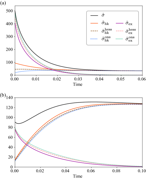
Figure 5: Comparison of three EPR decompositions. We calculate EPRs of the chemical reaction network in Eq. S93 for two distinct rate constants (detailed values are given in the text).

References

(1)
E. Aurell, C. Mejía-Monasterio, and P. Muratore-Ginanneschi, “Optimal
protocols and optimal transport in stochastic thermodynamics,”
Physical Review Letters, vol. 106, no. 25, p. 250601, 2011.
(2)
N. Shiraishi, K. Funo, and K. Saito, “Speed limit for classical stochastic
processes,” Physical review letters, vol. 121, no. 7, p. 070601,
2018.
(3)
T. R. Gingrich, J. M. Horowitz, N. Perunov, and J. L. England, “Dissipation
bounds all steady-state current fluctuations,” Physical Review
Letters, vol. 116, no. 12, p. 120601, 2016.
(4)
S.-i. Amari, Information geometry and its applications. Springer, 2016, vol. 194.
(5)
N. Ay, J. Jost, H. Vân Lê, and L. Schwachhöfer, Information
geometry. Springer, 2017, vol. 64.
(6)
M. Esposito and C. Van den Broeck, “Three detailed fluctuation theorems,”
Physical Review Letters, vol. 104, no. 9, p. 090601, 2010.
(7)
T. Hatano and S.-i. Sasa, “Steady-state thermodynamics of Langevin
systems,” Physical Review Letters, vol. 86, no. 16, p. 3463, 2001.
(8)
Y. Oono and M. Paniconi, “Steady state thermodynamics,” Progress of
Theoretical Physics Supplement, vol. 130, pp. 29–44, 1998.
(9)
D. Mandal and C. Jarzynski, “Analysis of slow transitions between
nonequilibrium steady states,” Journal of Statistical Mechanics:
Theory and Experiment, vol. 2016, no. 6, p. 063204, 2016.
(10)
C. Maes and K. Netočnỳ, “A nonequilibrium extension of the
Clausius heat theorem,” Journal of Statistical Physics, vol. 154,
no. 1, pp. 188–203, 2014.
(11)
T. S. Komatsu, N. Nakagawa, S.-i. Sasa, and H. Tasaki, “Steady-state
thermodynamics for heat conduction: microscopic derivation,” Physical
Review Letters, vol. 100, no. 23, p. 230602, 2008.
(12)
R. E. Spinney and I. J. Ford, “Nonequilibrium thermodynamics of stochastic
systems with odd and even variables,” Physical Review Letters, vol.
108, no. 17, p. 170603, 2012.
(13)
H. K. Lee, C. Kwon, and H. Park, “Fluctuation theorems and entropy production
with odd-parity variables,” Physical Review Letters, vol. 110, no. 5,
p. 050602, 2013.
(14)
K. Yoshimura, A. Kolchinsky, A. Dechant, and S. Ito, “Housekeeping and excess
entropy production for general nonlinear dynamics,” arXiv preprint
arXiv:2205.15227, 2022.
(15)
T. Sagawa and H. Hayakawa, “Geometrical expression of excess entropy
production,” Physical Review E, vol. 84, no. 5, p. 051110, 2011.
(16)
M. Esposito, U. Harbola, and S. Mukamel, “Entropy fluctuation theorems in
driven open systems: Application to electron counting statistics,”
Physical Review E, vol. 76, no. 3, p. 031132, 2007.
(17)
R. Rao and M. Esposito, “Nonequilibrium thermodynamics of chemical reaction
networks: wisdom from stochastic thermodynamics,” Physical Review X,
vol. 6, no. 4, p. 041064, 2016.
(18)
H. Ge and H. Qian, “Nonequilibrium thermodynamic formalism of nonlinear
chemical reaction systems with Waage–Guldberg’s law of mass action,”
Chemical Physics, vol. 472, pp. 241–248, 2016.
(19)
A. Dechant, S.-i. Sasa, and S. Ito, “Geometric decomposition of entropy
production in out-of-equilibrium systems,” Physical Review Research,
vol. 4, no. 1, p. L012034, 2022.
(20)
——, “Geometric decomposition of entropy production into excess,
housekeeping, and coupling parts,” Phys. Rev. E, vol. 106, p. 024125,
Aug 2022.
(21)
I. J. Ford and R. E. Spinney, “Entropy production from stochastic dynamics in
discrete full phase space,” Physical Review E, vol. 86, no. 2, p.
021127, 2012.
(22)
M. Nakazato and S. Ito, “Geometrical aspects of entropy production in
stochastic thermodynamics based on Wasserstein distance,” Physical
Review Research, vol. 3, no. 4, p. 043093, 2021.
(23)
F. Weinhold, “Metric geometry of equilibrium thermodynamics,” The
Journal of Chemical Physics, vol. 63, no. 6, pp. 2479–2483, 1975,
publisher: American Institute of Physics.
(24)
G. Ruppeiner, “Thermodynamics: A Riemannian geometric model,”
Physical Review A, vol. 20, no. 4, p. 1608, 1979, publisher: APS.
(25)
P. Salamon and R. S. Berry, “Thermodynamic length and dissipated
availability,” Physical Review Letters, vol. 51, no. 13, p. 1127,
1983.
(26)
F. Schlögl, “Thermodynamic metric and stochastic
measures,” Zeitschrift für Physik B
Condensed Matter, vol. 59, no. 4, pp. 449–454, Dec. 1985.
(27)
H. Janyszek, “Riemannian geometry and stability of thermodynamical equilibrium
systems,” Journal of Physics A: Mathematical and General, vol. 23,
no. 4, p. 477, 1990, publisher: IOP Publishing.
(28)
L. Diósi, K. Kulacsy, B. Lukács, and A. Rácz,
“Thermodynamic length, time, speed, and optimum path
to minimize entropy production,” The Journal
of Chemical Physics, vol. 105, no. 24, pp. 11 220–11 225, Dec. 1996.
(29)
R. Mrugala, J. D. Nulton, J. C. Schön, and P. Salamon,
“Statistical approach to the geometric structure of
thermodynamics,” Physical Review A,
vol. 41, no. 6, pp. 3156–3160, Mar. 1990.
(30)
D. Brody and N. Rivier, “Geometrical aspects of
statistical mechanics,” Physical Review E,
vol. 51, no. 2, pp. 1006–1011, Feb. 1995.
(31)
G. E. Crooks, “Measuring Thermodynamic Length,”
Physical Review Letters, vol. 99, no. 10,
Sep. 2007.
(32)
D. A. Sivak and G. E. Crooks, “Thermodynamic Metrics
and Optimal Paths,” Physical Review
Letters, vol. 108, no. 19, May 2012.
(33)
S. Ito, “Stochastic thermodynamic interpretation of information geometry,”
Physical Review Letters, vol. 121, no. 3, p. 030605, 2018.
(34)
T. Nakamura, H. Hasegawa, and D. Driebe, “Reconsideration of the generalized
second law based on information geometry,” Journal of Physics
Communications, vol. 3, no. 1, p. 015015, 2019.
(35)
S. Ito and A. Dechant, “Stochastic time evolution, information geometry, and
the Cramér-Rao bound,” Physical Review X, vol. 10, no. 2, p.
021056, 2020.
(36)
S. Ito, “Information geometry, trade-off relations, and generalized
Glansdorff–Prigogine criterion for stability,” Journal of Physics
A: Mathematical and Theoretical, vol. 55, no. 5, p. 054001, 2022.
(37)
A. Kolchinsky and D. H. Wolpert, “Work, entropy production, and thermodynamics
of information under protocol constraints,” Physical Review X,
vol. 11, no. 4, p. 041024, 2021.
(38)
K. Yoshimura and S. Ito, “Information geometric inequalities of chemical
thermodynamics,” Physical Review Research, vol. 3, no. 1, p. 013175,
2021.
(39)
N. Ohga and S. Ito, “Information-geometric Legendre duality in stochastic
thermodynamics,” arXiv preprint arXiv:2112.11008, 2021.
(40)
Y. Sughiyama, D. Loutchko, A. Kamimura, and T. J. Kobayashi, “Hessian
geometric structure of chemical thermodynamic systems with stoichiometric
constraints,” Phys. Rev. Research, vol. 4, p. 033065, Jul 2022.
(41)
N. Ohga and S. Ito, “Information-geometric structure for chemical
thermodynamics: An explicit construction of dual affine coordinates,”
Phys. Rev. E, vol. 106, p. 044131, Oct 2022.
(42)
T. J. Kobayashi, D. Loutchko, A. Kamimura, and Y. Sughiyama, “Kinetic
derivation of the hessian geometric structure in chemical reaction
networks,” Phys. Rev. Research, vol. 4, p. 033066, Jul 2022.
(43)
S. B. Nicholson, A. del Campo, and J. R. Green, “Nonequilibrium uncertainty
principle from information geometry,” Physical Review E, vol. 98,
no. 3, p. 032106, 2018.
(44)
N. Shiraishi and K. Saito, “Information-theoretical bound of the
irreversibility in thermal relaxation processes,” Physical Review
Letters, vol. 123, no. 11, p. 110603, 2019.
(45)
T. Van Vu and Y. Hasegawa, “Geometrical bounds of the irreversibility in
Markovian systems,” Physical Review Letters, vol. 126, no. 1, p.
010601, 2021.
(46)
S. Ito, M. Oizumi, and S.-i. Amari, “Unified framework for the entropy
production and the stochastic interaction based on information geometry,”
Physical Review Research, vol. 2, no. 3, p. 033048, 2020.
(47)
T. J. Kobayashi, D. Loutchko, A. Kamimura, and Y. Sughiyama, “Hessian geometry
of nonequilibrium chemical reaction networks and entropy production
decompositions,” Physical Review Research, vol. 4, no. 3, p. 033208,
2022.
(48)
J. Maas, “Gradient flows of the entropy for finite Markov chains,”
Journal of Functional Analysis, vol. 261, no. 8, pp. 2250–2292, Oct.
2011.
(49)
A. Mielke, “A gradient structure for reaction–diffusion systems and for
energy-drift-diffusion systems,” Nonlinearity, vol. 24, no. 4, p.
1329, 2011.
(50)
D.-K. Kim, Y. Bae, S. Lee, and H. Jeong, “Learning entropy production via
neural networks,” Physical Review Letters, vol. 125, no. 14, p.
140604, 2020.
(51)
S. Otsubo, S. Ito, A. Dechant, and T. Sagawa, “Estimating entropy production
by machine learning of short-time fluctuating currents,” Physical
Review E, vol. 101, no. 6, p. 062106, 2020.
(52)
T. Van Vu, Y. Hasegawa et al., “Entropy production estimation with
optimal current,” Physical Review E, vol. 101, no. 4, p. 042138,
2020.
(53)
A. Dechant, “Minimum entropy production, detailed balance and Wasserstein
distance for continuous-time Markov processes,” Journal of Physics
A: Mathematical and Theoretical, 2022.
(54)
J. M. Horowitz and T. R. Gingrich, “Thermodynamic uncertainty relations
constrain non-equilibrium fluctuations,” Nature Physics, vol. 16,
no. 1, pp. 15–20, 2020.
(55)
K. Yoshimura and S. Ito, “Thermodynamic uncertainty relation and thermodynamic
speed limit in deterministic chemical reaction networks,” Physical
Review Letters, vol. 127, no. 16, p. 160601, 2021.
(56)
R. Hamazaki, “Speed limits for macroscopic transitions,” PRX Quantum,
vol. 3, no. 2, p. 020319, 2022.
(57)
A. Bérut, A. Arakelyan, A. Petrosyan, S. Ciliberto, R. Dillenschneider, and
E. Lutz, “Experimental verification of Landauer’s principle linking
information and thermodynamics,” Nature, vol. 483, no. 7388, pp.
187–189, 2012.
(58)
Y.-Z. Zhen, D. Egloff, K. Modi, and O. Dahlsten, “Universal bound on energy
cost of bit reset in finite time,” Physical Review Letters, vol. 127,
no. 19, p. 190602, 2021.
(59)
——, “Inverse linear versus exponential scaling of work penalty in
finite-time bit reset,” Physical Review E, vol. 105, no. 4, p.
044147, 2022.
(60)
J.-C. Delvenne and G. Falasco, “The thermo-kinetic relations,” arXiv
preprint arXiv:2110.13050, 2021.
(61)
V. T. Vo, T. Van Vu, and Y. Hasegawa, “Unified approach to classical speed
limit and thermodynamic uncertainty relation,” Phys. Rev. E, vol.
102, p. 062132, Dec 2020.
(62)
J. S. Lee, S. Lee, H. Kwon, and H. Park, “Speed limit for a highly
irreversible process and tight finite-time Landauer’s bound,” Phys.
Rev. Lett., vol. 129, p. 120603, Sep 2022.
(63)
D. S. P. Salazar, “Lower bound for entropy production rate in stochastic
systems far from equilibrium,” Phys. Rev. E, vol. 106, p. L032101,
Sep 2022.
(64)
I. Prigogine and R. Lefever, “Symmetry breaking instabilities in dissipative
systems. II,” The Journal of Chemical Physics, vol. 48, no. 4, pp.
1695–1700, 1968.
(65)
R. E. Spinney and I. J. Ford, “Entropy production in full phase space for
continuous stochastic dynamics,” Physical Review E, vol. 85, no. 5,
p. 051113, 2012.
(66)
M. Collins, R. E. Schapire, and Y. Singer, “Logistic regression, AdaBoost
and Bregman distances,” Machine Learning, vol. 48, no. 1, pp.
253–285, 2002.
(67)
G. C. Calafiore and L. El Ghaoui, Optimization models. Cambridge university press, 2014.
(68)
W. Rudin, Principles of Mathematical Analysis, 3rd ed. New York: McGraw-Hill Education, Jan. 1976.
(69)
S. Otsubo, S. K. Manikandan, T. Sagawa, and S. Krishnamurthy, “Estimating
time-dependent entropy production from non-equilibrium trajectories,”
Communications Physics, vol. 5, no. 1, pp. 1–10, 2022.
(70)
C. Gardiner, Handbook of Stochastic
Methods: for Physics, Chemistry and the Natural Sciences,
3rd ed. Berlin ; New York: Springer,
Apr. 2004.
(71)
M. Esposito and C. Van den Broeck, “Three faces of the second law. I.
Master equation formulation,” Physical Review E, vol. 82, no. 1, p.
011143, 2010.
(72)
M. Feinberg, Foundations of Chemical Reaction Network Theory, ser.
Applied Mathematical Sciences. Cham: Springer International Publishing, 2019, vol. 202.