How should we proxy for race/ethnicity? Comparing Bayesian Improved Surname Geocoding to Machine Learning methods

Abstract

Bayesian Improved Surname Geocoding (BISG) is the most popular method for proxying race/ethnicity in voter registration files that do not contain it. This paper benchmarks BISG against a range of previously untested machine learning alternatives, using voter files with self-reported race/ethnicity from California, Florida, North Carolina, and Georgia. This analysis yields three key findings. First, machine learning consistently outperforms BISG at individual classification of race/ethnicity. Second, BISG and machine learning methods exhibit divergent biases for estimating regional racial composition. Third, the performance of all methods varies substantially across states. These results suggest that pre-trained machine learning models are preferable to BISG for individual classification. Furthermore, mixed results across states underscore the need for researchers to empirically validate their chosen race/ethnicity proxy in their populations of interest.

Keywords Imputation Methods  $\cdot$ Machine Learning  $\cdot$ Computational social science  $\cdot$ Bayesian imputation

1 Introduction

Political science research often requires constructing a race/ethnicity proxy variable for datasets that do not contain it, like voter registration files, lists of electoral candidates, or political donation records. Constructing such a proxy is an important step for conducting ecological inference in voting rights litigation (Barreto et al. (2019), Imai and Khanna (2016)), redistricting (DeLuca and Curiel (2022), Kenny et al. (2021)), and substantive research on the role of race/ethnicity in politics (Enos (2016), Enos et al. (2019), Grumbach and Sahn (2020)). The most common method for proxying race/ethnicity is Bayesian Improved Surname Geocoding (BISG), which uses Bayes’ rule to compute a probability distribution over race/ethnicity categories conditional on a voter’s surname and where they live (Elliott et al. (2008, 2009)). BISG has attained widespread popularity due to its parsimony, computational efficiency, and superior performance when compared to existing alternatives, namely spatial interpolation of Census racial-ethnic composition from Census geographies (Imai and Khanna (2016), Clark et al. (2021), Shah and Davis (2017)).

While BISG performs well compared to the small suite of existing alternatives, it has not yet been benchmarked against machine learning (ML) models, which can produce race/ethnicity predictions from more flexible and potentially more accurate models. In this paper I present the results of such a benchmark. I train a range of machine learning models using voter registration data from Florida, Georgia, North Carolina, and a portion of California where voters self-report their race/ethnicity upon registration. The registries in these states contain over 26 million labelled observations, which equates to greater than a five percent non-representative sample of the United States electorate. I then compare BISG against predictions from these models made out-of-state.

I find that machine learning models consistently outperform BISG at individual classification, and perform roughly as well at estimating precinct composition. Furthermore, the performance of all methods varies substantially across states and neighborhoods. This underscores the need for researchers to empirically validate their use of any race/ethnicity proxying method for each new application. I also discuss the implications of these results for existing and future research using race/ethnicity proxies.

2 Methods for imputing race/ethnicity

BISG and extensions

BISG computes the probability of race given a voter’s surname and geographic location, $P(R=r|S=s,G=g)$, using Bayes theorem. Assuming $P(G|R)\rotatebox[origin={c}]{90.0}{$\models$}P(S|R)$,

$$P(R=r|S=s,G=g)\propto P(G=g|R=r)P(R=r|S=s)$$ (1)

The probability $P(G=g|R=r)$ can be obtained from Census summary tables by taking the number of people of race/ethnicity $R=r$ in neighborhood $G=g$ divided by the total number of people of race/ethnicity $r$. Recent research has shown that the imputations become more accurate as the geographic areas used to define $G$ becomes smaller. Most performance gains are achieved by matching people to geographic areas by zip code, although the best results are still obtained by geocoding the data and matching voters to blocks (Clark et al. (2021)). In this paper I use block-level geographic information from 2020 Decennial Census throughout.

The probability of race given surname, $P(R=r|S=s)$, comes directly from the Census Bureau’s surname lists which contain the proportion of all Decennial Census respondents with each surname in each racial-ethnic category. I use the merge_surnames function from the wru package to match voters with the correct $P(R|S)$ (Khanna and Imai (2021)). I then compute posterior probability $P(R|G,S)$ by multiplying the two quantities together for each race category and dividing by the sum across all race categories to normalize. For comparison, I also use the wru package to perform BISG, and find that the results of my calculations match closely to the package (see appendices A and B).

Previous work to extend BISG has involved layering on additional assumptions that enable the inclusion of more information within the framework of the Bayes’ rule formula. Given a series of conditional independence assumptions, various extensions can be made by altering equation 1,

$$P(R=r|S=s,G=g,X=x,Y=y,...)\propto\\ P(G=g|R=r)(X=x|R=r)(Y=y|R=r)...P(R=r|S=s)$$ (2)

Where $X,Y$, and so on are any voter characteristics whose probability conditional on race is computed from available data. Previous work has taken this approach to add first names (Voicu (2018)), age, gender, and party affiliation (Imai and Khanna (2016)), each yielding better performance than when using surname and geography alone.

Here, in addition to BISG, I also consider an extended method that combines information about geographic, surname, middle name and first name using 2. For each, I construct four separate lookup tables containing their probability given race-ethnicity. Each of the four tables uses data from three of the four states. Then, to compute estimates in any given state, I use the probabilities from the lookup table that does not contain that state. Therefore, extensions of BISG make use of data from out-of-state.

Machine learning methods

In equations 1 and 2 every term used to generate predictions is known and no parameters are estimated prior to computing a prediction. This is an advantage of BISG – predictions follow directly from an application of Bayes Theorem and so require no information beyond indirect data from the Census Bureau. However, data do exist with which to estimate unknown parameters in a more flexible model. This fact motivates experimenting with alternative ways of predicting the probability distribution of race/ethnicity.

Here I consider what has become a standard suite of machine learning methods geared toward prediction problems (Hastie et al., 2001). First, I fit straightforward multinomial regression models, where the probabilistic inputs to BISG are instead summed together to generate predictions using weights learned from observed data. Second, I fit a multinomial regression adding an elasticnet penality term, which shrinks the learned weights in the model towards zero to reduce the risk of overfitting. Third, I fit random forests. Random forests average over multiple decision trees, each of which partitions subsets of observations into classification groups. Fourth, I fit gradient boosted decision trees, which greedily build random forests such that each subsequent tree minimizes the remaining loss from the previous combination of trees. These represent four of the most standard alternatives for multinomial classification tasks where prediction is the primary objective.

3 Data and methods

Using ML to proxy race/ethnicity carries a major risk of over-fitting to the characteristics of states for which labelled data is available. Existing research on ML for race-ethnicity classification has achieved exceptional performance when models are trained in the same geographic regions where they are tested (Sood and Laohaprapanon (2018), Lee et al. (2017)), but political scientists and practitioners do not need to impute the race/ethnicity of voters in the regions where race/ethnicity is already self-reported – they need to impute it in all other geographic regions of the United States. Furthermore, scholars have grown increasingly wary of machine learning applications across fields that show promising results but may later fail to replicate due to small methodological errors or slight changes in conditions (Kapoor and Narayanan, 2022).

To ensure a fair comparison between BISG and ML while accounting for the risk of over-fitting, I apply a maximally conservative ‘out-of-state’ evaluation strategy. All supervised models are trained using data from three states and used to generate predictions in the fourth. Thus, I apply these models in a different context with a different cultural and institutional history than where they were trained.

The potential for error due to over-fitting in this setting is further amplified by the relatively extreme racial and ethnic diversity of these four states. Georgia and North Carolina have among the largest Black population shares in the country, while California has the largest Asian share. Furthermore, although Florida and California are among the states with the largest Hispanic population share, their Hispanic populations are quite different. The largest inflows of Hispanics to Florida come from Cuba (41 percent), while Californian Hispanics are predominantly of Mexican origin (84 percent). To the extent that surname frequency differs across nationalities, this could pose challenges for models fit using surnames to predict race/ethnicity.

The data used for this analysis are voter registration records from Florida, Georgia, North Carolina, and California. The Florida and Georgia data were collected after the 2018 national election, North Carolina after the 2016 national election, and California after the 2020 election. For Florida, North Carolina, and Georgia, the data contain all registered voters and had already been geocoded as part of previous projects . For California, only roughly twenty percent of the voter file contains self-reported race-ethnicity. These data were obtained in raw format and roughly eighty percent of them were successfully geocoded using the Census Bureau’s geocoding API. The incompleteness of the California data should not meaningfully impact the conclusions in this paper, since my focus is on comparing methods for race-ethnicity imputation rather than downstream applications.

	Florida	Georgia	N. Carolina	California
N. obs	8,008,186	6,302,094	6,347,235	5,289,420
Prp. White	.687	.527	.684	.442
Prp. Black	.134	.301	.209	.052
Prp. Hispanic	.139	.034	.028	.232
Prp. Asian	.017	.024	.013	.159
Prp. Other	.023	.114	.066	.115
Mean Age	55.2	45.6	49.0	41.8
Prp. Male	.446	.465.	.442	.094
Prp. Female	.541	.533	.525	.083
Prp. Unknown	.013	.001	.032	.822

Table 1: Self-reported demographic characteristics of voters in Florida, Georgia, North Carolina, and a subset of voters from California.

Table 1 presents the aggregate demographic characteristics of the voters in each state after pre-processing. For all four states, the data contain voters’ first, middle, and last names, along with their gender, age, and self-reported race-ethnicity. The options for self-reporting race-ethnicity in all four states are White, Black, Hispanic, Asian, Other, and Unknown. For each dataset, voters without unique IDs and who could not be successfully geocoded were removed. All voters whose race was categorized as missing or ‘Unknown’ were also removed. I identified voters’ Census blocks of residence by using the sf package in R (Pebesma (2018)) to conduct spatial joins to 2020 block geographic regions using their geolocation.

I trained all model types described in section 2.2. I used the tidymodels framework in R to tune, train, and evaluate the models (Kuhn and Wickham, 2020). For each model type, I tuned and trained four separate models, each completely withholding data from one state. The model tuning procedure involved constructing a Latin hypercube grid of possible hyperparameter combinations and iterating over the grid using five-fold cross-validation to identify the best-performing combination. For this tuning procedure I used a random sample of the 100 thousand voters from the data. Then, using the best-performing set of hyperparameters from the tuning procedure, I trained each model on a one million-voter sample. I repeated this procedure twice using two different sets of predictors. First, I used only the ten probabilistic inputs to a basic BISG-based prediction. Second, I used an expanded set that also includes probabilistic inputs based on voters’ first and middle names. Finally, I used the trained models to generate predictions for all voters in each held-out state. I present an evaluation of these models compared to BISG in the next section.

4 Out-of-state validation

Here I compare the performance of different race/ethnicity proxy methods at the individual and aggregate level based on an out-of-state validation exercise. I tuned and trained each model four times, each time leaving out data from one of the four states. Using each of these models I generated predictions in the fourth, held-out state, and evaluated these predictions against self-reported race/ethnicity. I then compared the performance of each method against BISG.

The inputs to the different methods are exactly the same for all comparisons, meaning that the only difference between machine learning methods and BISG is the computations applied to those inputs to generate predictions. Furthermore, all ML models are evaluated out-of-state. For example, wherever performance is reported for an ML model in Florida, that model was trained using voter data from California, Georgia, and North Carolina, before being used to make predictions in Florida.

In the following subsections I present figures which summarize performance differences between BISG and ML models in general. For a more detailed comparison between models, appendices A and B contain tables with the specific values underlying these figures. From these appendices, two results are worth mentioning here. First, results using my implementation of BISG are similar to results when using the popular wru package.

Second, both BISG and ML approaches struggle with proxying the ‘other’ race/ethnicity category. For this class, area under the curve for individual classification ranges between 0.5 and 0.7 for most models, compared to .8 to 1 for the other race/ethnicities. The ‘other’ category may be difficult to model because it amalgamates a diverse group of individuals, including those who identify with more than one race/ethnicity. Researchers typically tolerate poor performance on the ‘other’ category because the group represents less than one percent of the population and because substantive questions usually pertain to the more well-defined groups.

Classifying individual voters

I first examined the overall performance of each method at classifying voter race/ethnicity. Figure 1 presents the area under the receiver operation curve (AUC) for all models by state, race, and set of inputs. Using a minimal set of inputs ($P(G|R)$ and $P(R|S)$), BISG’s performance compared to ML appears mixed, sometimes outperforming ML and sometimes not. When using the larger pool of inputs, ML models consistently outperform BISG. Notably, when using this larger set of inputs all ML methods cluster together and attain similar performance. This implies that even a simple switch from BISG to multinomial logistic regression can substantially improve individual predictions.

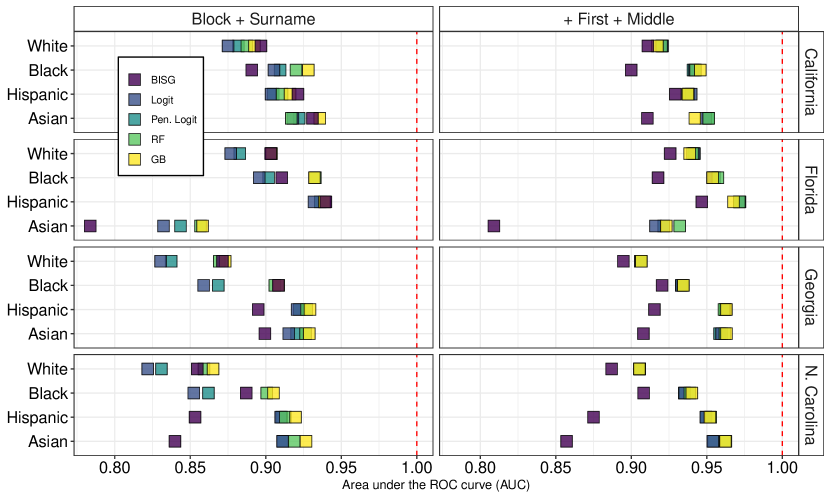
Figure 1: Comparison of area under the receiver operating curve (AUC) between BISG and ML methods. Left panels use probabilistic information about block and surname only. Right panels use these, plus information about first name and middle name. Machine learning models are trained on three states and used to generate predictions in the fourth.

Next, I examined the calibration of BISG and ML approaches. Figure 2 plots calibration curves for each method and each combination of state and race. A well-calibrated model will fall close the identity line. Being under the identity line means that too much probability is assigned to a given race/ethnicity, and being above it means not enough probability has been assigned.

In most cases, BISG appears equally or worse-calibrated than ML models, particularly for Asian and Hispanic voters. The one case where BISG appears better calibrated is for Asian voters in California. Both models do not assign enough probability to the Asian category for Californian voters, but the ML models appear more poorly calibrated than BISG. This poor calibration likely results from the relatively extreme size of the Asian population in California. ML models trained on other states are partially informed by the base rates of each race/ethnicity in each state, and California has the largest Asian share of any state in the country.

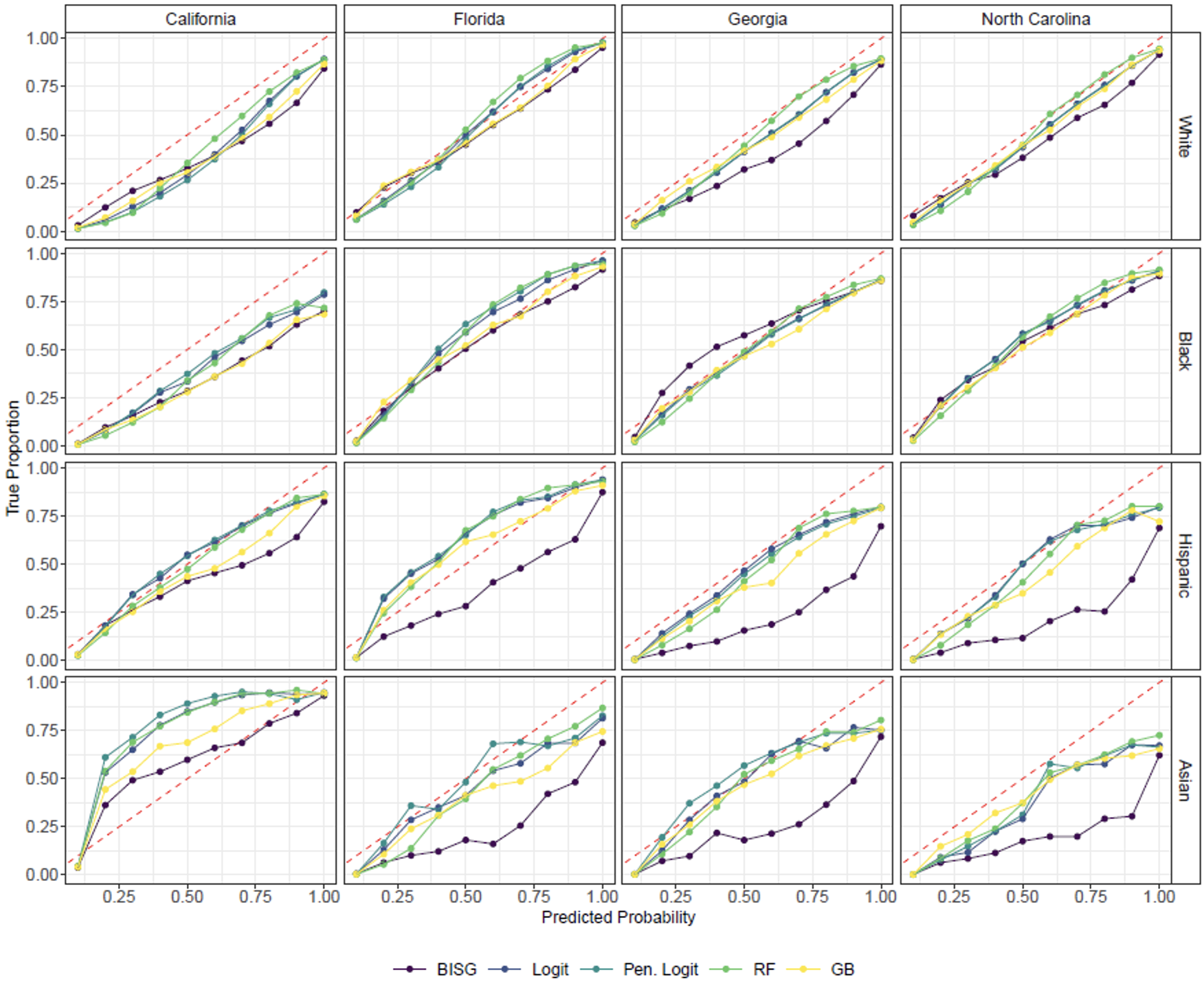
Figure 2: Calibration curves plotting the observed proportion of voters self-reporting with each race-ethnicity as a function of the predicted probabilities from each model. Both models use the full set of input data. The diagonal line indicates perfect calibration such that for any predicted probability, the actual proportion of voters with self-identifying with that race-ethnicity equals the predicted probability. All points calculated by taking the mean within bins equal to one tenth of the probability space.

In general, the calibration curves for the two methods appear on the same side of the identity line. The exception is for Hispanics in Florida, where BISG is over-calibrated and the supervised method is under-calibrated. It is unclear why BISG appears over-calibrated, though the under-calibration of the supervised method is likely again due to differences in the base-rate share of Hispanics in Florida compared to the other states under study.

Taken together, these results support the conclusion that for individual prediction, more highly parameterized models leveraging observed data should be used over BISG.

Estimating racial composition

Next, I evaluated the performance of supervised methods at estimating the racial composition of a geographic area. Although many applications require analyzing voter data at the precinct level, I follow Kenny et al. (2021) in conducting composition evaluations for tracts. Tracts are advantageous over precincts from an analytical perspective because they are of roughly equal size and are always nested inside counties and states. Furthermore, results at the tract level should be highly consistent with those at the precinct level.

Figure 3 summarizes the performance of each model for estimating tract racial/ethnic composition when using the larger set of inputs (First name, middle name, surname, block). In Georgia and North Carolina, ML models continue to outperform BISG in terms of overall error magnitude (RMSE) and bias. For Florida and California, however, results appear more mixed. BISG remains the best or one of the best methods for estimating racial composition in Florida, and in certain racial/ethnic categories in California.

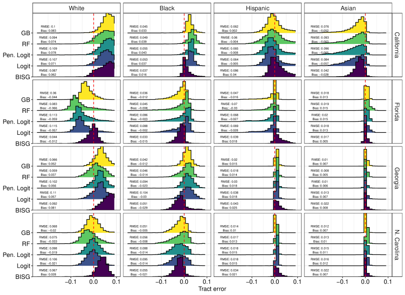
Figure 3: Density histograms of errors in estimation of tract-level racial/ethnic composition. Bins to the right of zero contain tracts for which a method has overestimated the share of voters of a given race/ethnicity, while bins to the left indicate underestimation. The RMSE and bias for each race-method-state combination are also presented.

Furthermore, figure 3 reveals meaningful variation in the bias of all methods across states. For instance, BISG performs well at estimating the share of white voters in each precinct in Florida, the setting for the canonical BISG validation study in political science (Imai and Khanna, 2016). In every other state, however, BISG consistently overestimates the white share of precincts. Similarly for Black voters, by looking at Florida, Georgia, and North Carolina one might conclude that BISG tends to underestimate the share of black voters in each precinct. If a researcher adopted this prior belief when applying estimating the Black share of voters in California, they might end up doubly wrong; BISG overestimates the Black share of voters in California, and a researcher might assume that even these must be underestimates, given the performance of BISG in other states.

5 Discussion

In this paper, I conducted the first direct comparison between BISG and ML methods for constructing a race/ethnicity proxy variable in voter registration data, using data from four states and evaluating the ML models on out-of-state performance. To the author’s knowledge, this is also the largest validation study for race/ethnicity proxy methods to date. The exercise has yielded three novel results. First, BISG and machine learning perform similarly for estimating aggregate racial/ethnic composition. Second, machine learning outperforms BISG at individual classification of race/ethnicity. Third, the performance of all methods varies substantially across states.

The first two points have clear implications for future research. When a researcher’s goal is to estimate the racial composition of a neighborhood or precinct, the evidence presented here suggests BISG is a good tool. While it does not perform best for every race/ethnicity in all of the tested states, it performs comparably or better in many instances. For individual prediction, results are less favorable to BISG. Provided researchers have access to individuals’ first and middle names, they should use ML models trained on available data from voter registries. ML consistently produced more accurate individual-level race/ethnicity proxies than BISG in every state for every race/ethnicity. Furthermore, ML methods were better-calibrated than BISG in every case except for Asians in California.

Another important finding from this benchmarking exercise is that race/ethnicity proxy methods, methods perform differently across states. For precinct composition estimation, patterns of over- or underestimation do not consistent across the country. As such, it may not be sufficient for researchers to rely on empirical validation studies in Florida (Imai and Khanna, 2016) or Georgia (Clark et al., 2021) when applying BISG in a novel context. Instead, researchers should seek to validate their use of any race/ethnicity metric in each new setting by collecting ground-truth race/ethnicity self-reports and using them for in a validation study.

Biased proxy variables can bias conclusions from downstream analyses, particularly when the bias is correlated with the outcome and predictor of interest Knox et al. (2022). Confidentiality requirements often prevent authors from publicizing raw individual-level data for research reliant on BISG. This largely prevents empirical assessments of how the results of previous research may be influenced by biases in proxied race/ethnicity. As a result, I can only speculate about the implications of the results above for existing and future research.

Two papers apply BISG in California, where the results above do suggest that BISG is biased. Enos, Kaufman, and Sands use BISG to construct inputs for ecological inference, to estimate changes in Black and white support for education policies as a result of the LA riots (Enos et al., 2019). The authors justify their use of BISG, in part, by citing the false positive rate for Black voters in Florida Imai and Khanna (2016). This argument does not hold given the results presented above, which show that while BISG provides fairly unbiased estimates of Black and white racial composition in Florida, it tends to overestimate both shares in California to varying degrees. The potential bias of the race/ethnicity proxy is not critical to the results of this paper since the estimated effect persists across both Black and white. However, it might perhaps cast some doubt on the relative size of the observed effects when decomposed by race/ethnicity.

Abbott and Magazinnik also use BISG in California to study the effect of a change from at-large to ward elections on the share of Latino candidates elected to school boards (Abott and Magazinnik, 2020). BISG is used to proxy the race/ethnicity of the candidates. The authors argue that BISG is not likely biased in this setting because the independence assumption almost certainly holds. The results presented in this paper show that, empirically, BISG’s predictions about Hispanic voters in California are biased. They overestimate the share of Hispanics in electoral precincts and over-assign probability to the Hispanic category in individual classification. For this application application, a pre-trained ML model would likely yield a more accurate proxy.

The authors model the proportion seats won by Hispanics in each school board in a two-way fixed effects regression analysis where the parameter of interest interacts the Hispanic share of the school district electorate with an indicator for the presence of ward elections. The results presented above suggest that the authors’ outcome of interest may be biased upward, which would not in itself affect their key estimates. However, if the bias towards overestimating Hispanic share is correlated across space with the Hispanic share of each school district, the estimated effect of switching to ward elections may also be biased.

Additionally, the authors show that the effect of changing to ward elections on the share of Hispanic election winners is concentrated within the most segregated school districts across the state. BISG is most accurate in segregated areas (Decter-Frain et al., 2022). The reported differences in the effects across districts with different levels of segregation may result from some combination of a real difference, and differences in the accuracy of BISG across segregated and diverse neighborhoods.

The above two examples illustrate the challenge of using race/ethnicity proxies in substantive research. In each case, concerns about the potential for biases to emerge from the proxy could be best addressed by manually labelling a small set of individuals and using them to compare methods and decide on the most accurate for the setting. In the latter case, the evidence presented in this paper suggests an ML model may provide more credible results than BISG.

Beyond these examples, BISG has been used in nationwide applications (Brown and Enos, 2021; Grumbach and Sahn, 2020) and has become increasingly common in redistricting (DeLuca and Curiel, 2022), and voting rights (Barreto et al., 2021). For each of these applications, BISG may or may not be the best method for constructing a proxy. The results I have presented here suggest that, in many cases, a machine learning model pre-trained on labelled observations from California, Florida, Georgia, and North Carolina may provide more accurate, better calibrated results.

Appendix A Full individual-level results

		Block + Surname								+ First + Middle
State	Race/Eth	WRU	BISG	Logit	Logit2	ELNET	RF	GB		BISG	Logit	Logit2	ELNET	RF	GB
California
	White	0.893	0.897	0.875	0.873	0.882	0.887	0.892		0.911	0.921	0.921	0.921	0.920	0.917
	Black	0.878	0.891	0.905	0.895	0.909	0.920	0.928		0.900	0.942	0.945	0.941	0.943	0.946
	Hispanic	0.915	0.921	0.903	0.905	0.905	0.911	0.916		0.929	0.940	0.941	0.938	0.937	0.938
	Asian	0.916	0.931	0.918	0.910	0.922	0.917	0.936		0.911	0.949	0.953	0.951	0.951	0.942
	Other	0.527	0.524	0.508	0.512	0.513	0.508	0.512		0.547	0.556	0.538	0.554	0.537	0.546
Florida
	White	0.899	0.903	0.877	0.862	0.883	0.903	0.904		0.926	0.942	0.942	0.942	0.941	0.939
	Black	0.909	0.911	0.896	0.877	0.902	0.933	0.932		0.918	0.954	0.957	0.955	0.957	0.954
	Hispanic	0.932	0.940	0.932	0.930	0.936	0.939	0.939		0.947	0.972	0.972	0.972	0.971	0.968
	Asian	0.778	0.784	0.832	0.844	0.844	0.857	0.858		0.809	0.916	0.929	0.921	0.932	0.923
	Other	0.575	0.576	0.591	0.593	0.605	0.580	0.587		0.591	0.662	0.646	0.665	0.644	0.633
Georgia
	White	0.867	0.871	0.830	0.793	0.837	0.869	0.873		0.895	0.906	0.907	0.906	0.907	0.907
	Black	0.904	0.908	0.859	0.815	0.869	0.906	0.909		0.920	0.933	0.934	0.933	0.934	0.934
	Hispanic	0.873	0.895	0.921	0.929	0.922	0.927	0.929		0.915	0.962	0.964	0.962	0.961	0.963
	Asian	0.878	0.899	0.915	0.927	0.920	0.926	0.929		0.908	0.960	0.964	0.958	0.962	0.963
	Other	0.531	0.525	0.542	0.555	0.544	0.550	0.550		0.540	0.566	0.577	0.561	0.572	0.569
N. Carolina
	White	0.853	0.855	0.822	0.790	0.831	0.859	0.865		0.887	0.905	0.906	0.906	0.906	0.905
	Black	0.889	0.887	0.852	0.821	0.862	0.901	0.905		0.908	0.935	0.940	0.935	0.939	0.940
	Hispanic	0.833	0.853	0.910	0.912	0.911	0.913	0.920		0.875	0.949	0.952	0.949	0.953	0.952
	Asian	0.817	0.840	0.911	0.915	0.911	0.919	0.927		0.857	0.954	0.961	0.954	0.963	0.962
	Other	0.571	0.555	0.587	0.594	0.596	0.595	0.605		0.569	0.600	0.627	0.599	0.643	0.634

Table 2: Area under the curve (AUC) for each model for each race in each state.

Appendix B Full precinct-level results

		Block + Surname								+ First + Middle
State	Race/Eth	BISG	WRU	ELNET	Logit	Logit2	RF	GB		BISG	ELNET	Logit	Logit2	RF	GB
California
	White	.087	.1	.121	.121	.136	.107	.112		.088	.083	.074	.071	.075	.087
	Black	.036	.042	.066	.064	.063	.053	.051		.029	.034	.032	.025	.039	.030
	Hispanic	.070	.072	.055	.051	.056	.050	.050		.064	.048	.049	.045	.045	.047
	Asian	.039	.044	.117	.102	.106	.103	.091		.041	.084	.073	.067	.094	.067
	Other	.113	.113	.083	.082	.083	.084	.088		.105	.083	.083	.083	.080	.095
Florida
	White	.045	.049	.143	.148	.162	.094	.075		.037	.066	.063	.058	.078	.044
	Black	.038	.046	.101	.106	.125	.039	.035		.035	.044	.042	.036	.044	.035
	Hispanic	.032	.029	.074	.077	.078	.066	.048		.029	.037	.033	.032	.052	.029
	Asian	.018	.017	.024	.021	.024	.021	.023		.010	.010	.010	.008	.014	.008
	Other	.016	.012	.075	.075	.075	.090	.063		.015	.075	.074	.070	.090	.055
Georgia
	White	.097	.115	.130	.141	.184	.070	.078		.087	.046	.046	.047	.038	.049
	Black	.059	.077	.120	.132	.177	.056	.052		.034	.029	.029	.027	.027	.022
	Hispanic	.046	.045	.030	.039	.023	.021	.023		.026	.015	.012	.009	.012	.012
	Asian	.025	.024	.012	.014	.013	.009	.011		.017	.006	.010	.008	.006	.008
	Other	.092	.092	.067	.065	.063	.056	.068		.092	.070	.068	.064	.051	.073
N. Carolina	White	.044	.057	.109	.120	.149	.069	.058		.051	.038	.039	.041	.044	.037
	Black	.041	.051	.093	.104	.129	.038	.033		.034	.042	.041	.033	.040	.032
	Hispanic	.039	.035	.022	.022	.020	.019	.017		.017	.010	.010	.006	.010	.006
	Asian	.024	.023	.016	.017	.015	.013	.012		.014	.009	.011	.007	.010	.006
	Other	.046	.049	.050	.052	.051	.050	.047		.044	.051	.050	.044	.049	.043

Table 3: RMSE values for every model-race-state combination. All calculations weight by tract size.

		Block + Surname								+ First + Middle
State	Race/Eth	BISG	WRU	ELNET	Logit	Logit2	RF	GB		BISG	ELNET	Logit	Logit2	RF	GB
California
	White	.070	.079	.085	.079	.093	.095	.100		.075	.072	.062	.059	.061	.078
	Black	.018	.016	.058	.050	.043	.042	.039		.013	.030	.028	.021	.035	.026
	Hispanic	.031	.027	-.015	-.012	-.016	-.014	-.012		.025	-.002	.000	.004	.000	.007
	Asian	-.029	-.032	-.082	-.072	-.075	-.076	-.070		-.032	-.065	-.057	-.048	-.066	-.047
	Other	-.091	-.090	-.046	-.045	-.045	-.047	-.057		-.081	-.036	-.033	-.035	-.031	-.064
Florida
	White	-.013	.002	-.084	-.081	-.081	-.079	-.061		-.005	-.051	-.049	-.046	-.064	-.032
	Black	-.013	-.018	.014	.019	.014	.002	-.004		-.015	-.008	-.009	-.012	-.011	-.016
	Hispanic	.014	.008	-.025	-.027	-.026	-.026	-.015		.015	-.017	-.017	-.013	-.021	-.010
	Asian	.009	.009	.021	.018	.020	.018	.020		.003	.006	.005	.004	.010	.006
	Other	.002	-.001	.073	.072	.073	.086	.060		.002	.070	.070	.067	.086	.051
Georgia
	White	.086	.100	.082	.085	.078	.056	.068		.079	.033	.033	.034	.018	.039
	Black	-.041	-.049	-.060	-.069	-.058	-.034	-.035		-.016	.017	.014	.013	.009	.012
	Hispanic	.030	.025	.023	.024	.022	.018	.019		.016	.010	.009	.006	.010	.009
	Asian	.010	.009	.010	.010	.012	.005	.009		.006	.002	.004	.002	.004	.005
	Other	-.085	-.085	-.056	-.051	-.053	-.046	-.060		-.085	-.062	-.060	-.055	-.041	-.065
N. Carolina	White	.023	.035	-.042	-.045	-.045	-.050	-.038		.040	.001	.001	.003	-.016	-.001
	Black	-.025	-.028	-.005	-.004	.000	.000	.001		-.021	-.022	-.022	-.018	-.018	-.016
	Hispanic	.028	.023	.021	.022	.020	.018	.015		.012	.009	.009	.005	.009	.004
	Asian	.010	.010	.015	.016	.014	.012	.009		.004	.007	.007	.004	.008	.004
	Other	-.035	-.040	.011	.012	.011	.021	.013		-.035	.005	.005	.006	.017	.009

Table 4: Bias values for every model-race-state combination. All calculations weight by tract size.

References

- Barreto et al. [2019] Matt Barreto, Loren Collingwood, Sergio Garcia-Rios, and Kassra AR Oskooii. Estimating Candidate Support in Voting Rights Act Cases: Comparing Iterative EI and EI-R×C Methods. Sociological Methods & Research, page 004912411985239, July 2019. ISSN 0049-1241, 1552-8294. doi:10.1177/0049124119852394. URL http://journals.sagepub.com/doi/10.1177/0049124119852394.
- Imai and Khanna [2016] Kosuke Imai and Kabir Khanna. Improving Ecological Inference by Predicting Individual Ethnicity from Voter Registration Records. Political Analysis, 24(2):263–272, 2016. ISSN 1047-1987, 1476-4989. doi:10.1093/pan/mpw001. URL https://www.cambridge.org/core/product/identifier/S1047198700010962/type/journal_article.
- DeLuca and Curiel [2022] Kevin DeLuca and John A. Curiel. Validating the Applicability of Bayesian Inference with Surname and Geocoding to Congressional Redistricting. Political Analysis, pages 1–7, 2022.
- Kenny et al. [2021] Christopher T. Kenny, Shiro Kuriwaki, Cory McCartan, Evan T. R. Rosenman, Tyler Simko, and Kosuke Imai. The use of differential privacy for census data and its impact on redistricting: The case of the 2020 U.S. Census. Science Advances, 7(41):eabk3283, October 2021. ISSN 2375-2548. doi:10.1126/sciadv.abk3283. URL https://www.science.org/doi/10.1126/sciadv.abk3283.
- Enos [2016] Ryan D. Enos. What the Demolition of Public Housing Teaches Us about the Impact of Racial Threat on Political Behavior. American Journal of Political Science, 60(1):123–142, January 2016. ISSN 0092-5853, 1540-5907. doi:10.1111/ajps.12156. URL https://onlinelibrary.wiley.com/doi/10.1111/ajps.12156.
- Enos et al. [2019] Ryan D. Enos, Aaron R. Kaufman, and Melissa L. Sands. Can Violent Protest Change Local Policy Support? Evidence from the Aftermath of the 1992 Los Angeles Riot. American Political Science Review, 113(4):1012–1028, November 2019. ISSN 0003-0554, 1537-5943. doi:10.1017/S0003055419000340. URL https://www.cambridge.org/core/product/identifier/S0003055419000340/type/journal_article.
- Grumbach and Sahn [2020] Jacob M. Grumbach and Alexander Sahn. Race and Representation in Campaign Finance. American Political Science Review, 114(1):206–221, February 2020. ISSN 0003-0554, 1537-5943. doi:10.1017/S0003055419000637. URL https://www.cambridge.org/core/product/identifier/S0003055419000637/type/journal_article.
- Elliott et al. [2008] Marc N. Elliott, Allen Fremont, Peter A. Morrison, Philip Pantoja, and Nicole Lurie. A New Method for Estimating Race/Ethnicity and Associated Disparities Where Administrative Records Lack Self-Reported Race/Ethnicity: New Method for Estimating Race/Ethnicity and Associated Disparities. Health Services Research, 43(5p1):1722–1736, May 2008. ISSN 00179124, 14756773. doi:10.1111/j.1475-6773.2008.00854.x. URL https://onlinelibrary.wiley.com/doi/10.1111/j.1475-6773.2008.00854.x.
- Elliott et al. [2009] Marc N. Elliott, Peter A. Morrison, Allen Fremont, Daniel F. McCaffrey, Philip Pantoja, and Nicole Lurie. Using the Census Bureau’s surname list to improve estimates of race/ethnicity and associated disparities. Health Services and Outcomes Research Methodology, 9(2):69–83, June 2009. ISSN 1387-3741, 1572-9400. doi:10.1007/s10742-009-0047-1. URL http://link.springer.com/10.1007/s10742-009-0047-1.
- Clark et al. [2021] Jesse T. Clark, John A. Curiel, and Tyler S. Steelman. Minmaxing of Bayesian Improved Surname Geocoding and Geography Level Ups in Predicting Race. Political Analysis, pages 1–7, November 2021. ISSN 1047-1987, 1476-4989. doi:10.1017/pan.2021.31. URL https://www.cambridge.org/core/product/identifier/S1047198721000310/type/journal_article.
- Shah and Davis [2017] Paru R. Shah and Nicholas R. Davis. Comparing Three Methods of Measuring Race/Ethnicity. The Journal of Race, Ethnicity, and Politics, 2(1):124–139, March 2017. ISSN 2056-6085. doi:10.1017/rep.2016.27. URL https://www.cambridge.org/core/product/identifier/S2056608516000271/type/journal_article.
- Khanna and Imai [2021] Kabir Khanna and Kosuke Imai. wru: Who are You? Bayesian Prediction of Racial Category Using Surname and Geolocation, 2021. URL https://CRAN.R-project.org/package=wru. R package version 0.1-12.
- Voicu [2018] Ioan Voicu. Using First Name Information to Improve Race and Ethnicity Classification. Statistics and Public Policy, 5(1):1–13, January 2018. ISSN 2330-443X. doi:10.1080/2330443X.2018.1427012. URL https://www.tandfonline.com/doi/full/10.1080/2330443X.2018.1427012.
- Hastie et al. [2001] Trevor Hastie, Robert Tibshirani, and Jerome Friedman. The Elements of Statistical Learning. Springer Series in Statistics. Springer New York Inc., New York, NY, USA, 2001.
- Sood and Laohaprapanon [2018] Gaurav Sood and Suriyan Laohaprapanon. Predicting Race and Ethnicity From the Sequence of Characters in a Name. arXiv:1805.02109 [stat], May 2018. URL http://arxiv.org/abs/1805.02109. arXiv: 1805.02109.
- Lee et al. [2017] Jinhyuk Lee, Hyunjae Kim, Miyoung Ko, Donghee Choi, Jaehoon Choi, and Jaewoo Kang. Name Nationality Classification with Recurrent Neural Networks. In Proceedings of the Twenty-Sixth International Joint Conference on Artificial Intelligence, pages 2081–2087, Melbourne, Australia, August 2017. International Joint Conferences on Artificial Intelligence Organization. ISBN 978-0-9992411-0-3. doi:10.24963/ijcai.2017/289. URL https://www.ijcai.org/proceedings/2017/289.
- Kapoor and Narayanan [2022] Sayash Kapoor and Arvind Narayanan. Leakage and the Reproducibility Crisis in ML-based Science, July 2022. URL http://arxiv.org/abs/2207.07048. arXiv:2207.07048 [cs, stat].
- Decter-Frain et al. [2022] Ari Decter-Frain, Pratik Sachdeva, Loren Collingwood, Juandalyn Burke, Hikari Murayama, Matt Barreto, Scott Henderson, Spencer A Wood, and Joshua Zingher. Comparing Methods for Estimating Demographics in Racially Polarized Voting Analyses. preprint, SocArXiv, April 2022. URL https://osf.io/e854z.
- Pebesma [2018] Edzer Pebesma. Simple Features for R: Standardized Support for Spatial Vector Data. The R Journal, 10(1):439–446, 2018. doi:10.32614/RJ-2018-009. URL https://doi.org/10.32614/RJ-2018-009.
- Kuhn and Wickham [2020] Max Kuhn and Hadley Wickham. Tidymodels: a collection of packages for modeling and machine learning using tidyverse principles., 2020. URL https://www.tidymodels.org.
- Knox et al. [2022] Dean Knox, Christopher Lucas, and Wendy K. Tam Cho. Testing Causal Theories with Learned Proxies. Annual Review of Political Science, 25(1):419–441, May 2022. ISSN 1094-2939, 1545-1577. doi:10.1146/annurev-polisci-051120-111443. URL https://www.annualreviews.org/doi/10.1146/annurev-polisci-051120-111443.
- Abott and Magazinnik [2020] Carolyn Abott and Asya Magazinnik. At-Large Elections and Minority Representation in Local Government. American Journal of Political Science, 64(3):717–733, July 2020. ISSN 0092-5853, 1540-5907. doi:10.1111/ajps.12512. URL https://onlinelibrary.wiley.com/doi/10.1111/ajps.12512.
- Brown and Enos [2021] Jacob R. Brown and Ryan D. Enos. The measurement of partisan sorting for 180 million voters. Nature Human Behaviour, 5(8):998–1008, August 2021. ISSN 2397-3374. doi:10.1038/s41562-021-01066-z. URL https://www.nature.com/articles/s41562-021-01066-z.
- Barreto et al. [2021] Matthew Barreto, Michael Cohen, Loren Collingwood, Chad Dunn, and Sonni Waknin. A Novel Method for Showing Racially Polarized Voting: Bayesian Improved Surname Geocoding. SSRN Electronic Journal, 2021. ISSN 1556-5068. doi:10.2139/ssrn.3834818. URL https://www.ssrn.com/abstract=3834818.