Notes on Pseudo Entropy Amplification

Yutaka Ishiyama¹, Riku Kojima^1,2, Sho Matsui¹, and Kotaro Tamaoka¹

¹Department of Physics, College of Humanities and Sciences, Nihon University,
Sakura-josui, Tokyo 156-8550, Japan
²Research Center for Nuclear Physics (RCNP), Osaka University,
Ibaraki 567-0048, Japan.

1 Introduction and Summary

Quantum entanglement is a key concept to understanding various aspects of physics, including resources of quantum computation [1], critical phenomena [2, 3], topological phases [4, 5], and the emergence of spacetime in holography [6, 7, 8, 9, 10, 11, 12, 13]. The entanglement entropy, von Neumann entropy of the reduced density matrix, is one of the most fundamental measures to quantify the quantum entanglement for the bipartite pure state.

Recently, two states generalization of the entanglement entropy has been introduced, called pseudo entropy [14]. Let two states $\ket{\psi},\ket{\varphi}$ belong to a bipartite Hilbert space $\mathcal{H}_{A}\otimes\mathcal{H}_{B}$. Pseudo entropy is defined as von Neumann entropy associated with reduced transition matrix,

$$S(\tau^{\psi|\varphi}_{A})=-\mathrm{Tr}_{A}\left(\tau^{\psi|\varphi}_{A}\log\tau^{\psi|\varphi}_{A}\right),$$ (1)

where the (reduced) transition matrix is given by

$$\tau^{\psi|\varphi}_{A} =\mathrm{Tr}_{B}\,\tau^{\psi|\varphi},$$ (2)

$$\tau^{\psi|\varphi} =\dfrac{|\psi\rangle\langle\varphi|}{\langle\varphi|\psi\rangle}.$$ (3)

If the two states are the same, $\psi=\varphi$, the pseudo entropy reduces to the entanglement entropy for subsystem $A$. Importantly, we assume the two states have non-trivial overlap, $\langle\varphi|\psi\rangle\neq 0$. The pseudo entropy has been found to be a natural generalization of holographic entanglement entropy [6, 7, 8], which is dual to area of the minimal surface in the Euclidean time-dependent backgrounds.

Since the transition matrix is non-Hermitian, pseudo entropy can take complex values in general. Nevertheless, we have a nice quantum information theoretic interpretation for the real part: the real part of pseudo entropy can be identified with the number of distillable EPR pairs when averaging over intermediate states for fixed initial and final states. (Refer to [14, 15] for more details.) There are several applications of pseudo entropy in literature. One can use the pseudo entropy as a diagnosis of whether two states belong to the same quantum phase or not [16, 17, 18]. The entanglement entropy for non-Hermitian systems [19] can be understood as a concrete example of pseudo entropy as the left and right energy eigenstates are different in non-Hermitian Hamiltonians. Other interesting applications include the characterization of entanglement Hamiltonian [20] and gravitational setup with the absence of the time reflection symmetry [21, 15]. Refer also to further developments relevant to the pseudo entropy [22, 23, 24, 25].

It is well-known that von Neumann entropy is bounded above by the logarithm of the dimension of the Hilbert space $\log\dim\mathcal{H}$. On the other hand, pseudo entropy $S(\tau^{\psi|\varphi}_{A})$ can be larger than $\log\dim\mathcal{H}_{A}$. We will call this property amplification of pseudo entropy. Note that this amplification is also relevant to the classification of quantum phases [16, 17, 18] mentioned above.

In this paper, we study such amplification by focusing on a typical situation where two states $\ket{\psi},\ket{\varphi}$ have a small but non-zero overlap. Similar amplification can occur for the quantity called weak value [26, 27],

$$\mathrm{Tr}(\tau^{\psi|\varphi}\mathcal{O})=\dfrac{\langle\varphi|\mathcal{O}|\psi\rangle}{\langle\varphi|\psi\rangle},$$ (4)

where the transition matrices naturally appear. The weak value of $\mathcal{O}$ can also take a larger value than the maximum eigenvalue of $\mathcal{O}$. However, this is not always the case even if $\braket{\varphi}{\psi}$ is small. We study the similar setup in qubit systems (section 2), two-dimensional free CFT (section 3) and two-dimensional holographic CFT (section 4). Notably, while we observe the amplification in qubit systems and free CFT, we do not see it in holographic CFT as long as non-perturbative contributions are negligible.

The organization of the rest of this paper is as follows. In section 2, we study pseudo entropy amplification in qubit systems and discuss heuristic criteria for when pseudo entropy can (and cannot) be amplified. In section 3, we study amplification in two-dimensional free CFT. In section 4, we study (non-)amplification in two-dimensional holographic CFT. In section 5, we conclude and discuss future prospects.

Note added: While we were finalizing this paper, we became aware of [25] where the authors study the time-evolution of pseudo entropy by quench with the linear combination of operators in 2D CFTs. Although our motivation and parameter regime of interest are different from their paper, there are overlaps with our section 3.

2 Amplification in Qubit Systems

In this section, we first discuss qubit systems as an warm up exercise. Let us consider Bell states (EPR pairs),

$$\ket{\Phi^{\pm}} =\dfrac{1}{\sqrt{2}}(\ket{0_{A}0_{B}}\pm\ket{1_{A}1_{B}}),$$ (5)

$$\ket{\Psi^{\pm}} =\dfrac{1}{\sqrt{2}}(\ket{0_{A}1_{B}}\pm\ket{1_{A}0_{B}}).$$ (6)

In particular, these states are orthogonal to each other. In what follows, we will utilize $\ket{\Phi^{\pm}}$. We can repeat the same discussion for any different choice of two of four Bell states. The important point here is that these two states are both entangled states and orthogonal to each other. We cannot define transition matrix between these two states as we have no probability of transition from one state to another. Nevertheless, we can perturb one of two Bell states such that

$$\ket{\psi} =\ket{\Phi^{+}}+\epsilon\ket{\Phi^{-}},$$ (7)

$$\ket{\varphi} =\ket{\Phi^{-}},$$ (8)

then we have small but non-zero overlap, $\langle\varphi|\psi\rangle=\epsilon$. Namely, we will consider a formal rare process $\psi\rightarrow\varphi$ that potentially amplifies the weak value as we make the parameter $\epsilon$ smaller. As we will see soon, it is also the case for pseudo entropy. Although this setting may seem somewhat artificial, we choose it because it is convenient for comparison with calculations in field theories.

The transition matrix then has the following form,

$$\tau^{\psi|\varphi}_{A}=\dfrac{1+\epsilon}{2\epsilon}|0\rangle_{A}\langle 0|-\dfrac{1-\epsilon}{2\epsilon}|1\rangle_{A}\langle 1|.$$ (9)

We stress again that we cannot define the transition matrix at the exact $\epsilon=0$ point. Nevertheless, we can imagine small but nonzero $\epsilon$ so that the resulting weak value can be amplified by the parameter $\epsilon^{-1}$. The pseudo entropy gives

$$S(\tau^{\psi|\varphi}_{A})=-\dfrac{1+\epsilon}{2\epsilon}\log\left(\dfrac{1+\epsilon}{2\epsilon}\right)-\dfrac{\epsilon-1}{2\epsilon}\log\left(\dfrac{\epsilon-1}{2\epsilon}\right).$$ (10)

Obviously, the pseudo entropy is amplified as we make $\epsilon$ smaller. See Figure 1.

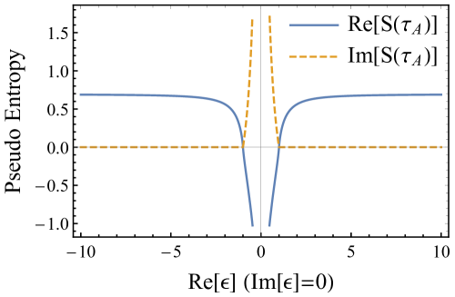
(a) $\textrm{Im}(\epsilon)=0$

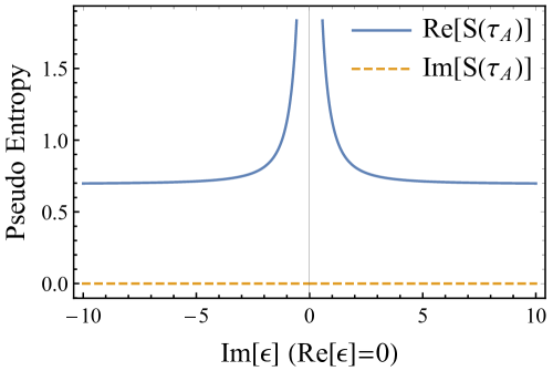
(b) $\textrm{Re}(\epsilon)=0$

Figure 1: Amplification of pseudo entropy for the states (5) and (6). Here we show the case $\epsilon$ is (a) real or (b) pure imaginary. In the case (b), the real-valuedness comes from a pair of eigenvalues that are complex conjugates of each other. It is useful to note that the lower or upper bound of the real part is given by $\log 2$ as $|\epsilon|\rightarrow\infty$ limit corresponds to the limit $\psi\rightarrow\varphi$.

As is the entanglement entropy, we can also define the pseudo Rényi entropy,

$$S^{(n)}(\tau^{\psi|\varphi}_{A})=\dfrac{\log\mathrm{Tr}_{A}\,(\tau^{\psi|\varphi}_{A})^{n}}{1-n}.$$ (11)

In general, the transition matrix is no longer Hermitian, so not guaranteed to be diagonalizable. Even in such cases, we can still define trace of such matrices. Thus, strictly speaking, we have to first define the Rényi version (11) and then define the pseudo entropy as $n\rightarrow 1$ limit.

For our later convenience, we note the second Rényi result,

$$S^{(2)}(\tau^{\psi|\varphi}_{A})=\log\left(\dfrac{2\epsilon^{2}}{1+\epsilon^{2}}\right).$$ (12)

Notice that detailed property of the amplification is quite different for each value of $n$ (See Figure 2). In this paper, we will mainly focus on whether pseudo entropy is amplified or not. In the current example, we see large amplifications of magnitude of $\mathrm{Re}[S^{(n)}]$ for any positive $n$.

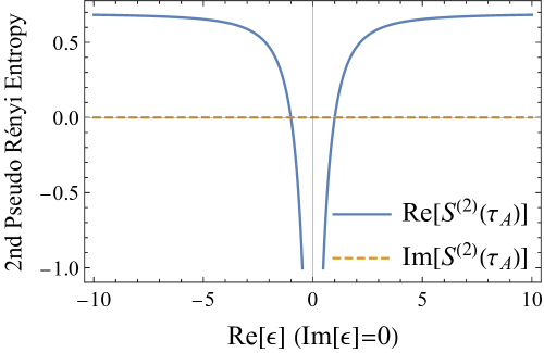
(a) $\textrm{Im}(\epsilon)=0$

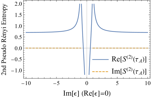
(b) $\textrm{Re}(\epsilon)=0$

Figure 2: Amplification of the second pseudo Rényi entropy for the states (5) and (6). Again we show the case $\epsilon$ is (a) real or (b) pure imaginary. In the case (b) with $|\epsilon|<1$, we have $\mathrm{Im}S^{(2)}=\pi$.

Amplification and weak value

We would like to stress that two entangled states with small overlap does not necessarily imply the amplification. This is similar to the amplification of weak value,

$$\mathrm{Tr}(\tau^{\psi|\varphi}\hat{A})=\dfrac{\langle\psi|\hat{A}|\varphi\rangle}{\langle\psi|\varphi\rangle}.$$ (13)

If neither initial nor finial states are eigenstates of the observable $\hat{A}$, one can amplify the weak value. Let us see examples as an illustration. Let $X$ be a spin flip operator, $X|0\rangle=|1\rangle,X|1\rangle=|0\rangle$ and $Z$ be a phase operator, $Z|0\rangle=|0\rangle,Z|1\rangle=-|1\rangle$. If we choose $\hat{A}=X\otimes X$, the weak value (13) amplifies with respect to $\epsilon$. On the other hand, if $\hat{A}=Z\otimes Z$, the weak value does not amplify since both of two states are eigenstates of $Z\otimes Z$.

The pseudo entropy indeed shares the similar property. In the previous example, two states are not left/right eigenstates of the reduced transition matrix (or “modular Hamiltonian”) thereof,

$$(\tau_{A}^{\psi|\varphi})^{\dagger}|\varphi\rangle\neq\alpha_{\varphi}|\varphi\rangle,\;\tau_{A}^{\psi|\varphi}|\psi\rangle\neq\alpha_{\psi}|\psi\rangle.$$ (14)

For the sake of comparison, let us consider a three qubit example,

$$\ket{\psi} =\ket{\Phi^{+}}\ket{0}+\epsilon\ket{\Phi^{+}}\ket{1},$$ (15)

$$\ket{\varphi} =\ket{\Phi^{+}}\ket{1}.$$ (16)

In this case, the orthogonality stems from a decoupled sector, not relevant to the quantum entanglement, (e.g. super selection sector). One can easily check that

$$\tau_{AC}^{\psi|\varphi}=\dfrac{I_{A}}{2}\otimes\left(\dfrac{1}{\epsilon}\ket{0}_{C}\bra{1}+\ket{1}_{C}\bra{1}\right)$$ (17)

and

$$(\tau_{AC}^{\psi|\varphi})^{\dagger}|\varphi\rangle=\dfrac{1}{2}|\varphi\rangle,\;\tau_{AC}^{\psi|\varphi}|\psi\rangle=\dfrac{1}{2}|\psi\rangle.$$ (18)

In this example, indeed we do not see the amplification,

$$S^{(n)}(\tau_{AC}^{\psi|\varphi})=S^{(n)}(\tau_{A}^{\psi|\varphi})=\log 2.$$ (19)

As we will see later, the holographic pseudo entropy has rather a similar structure to the latter example.

3 Amplification in 2D Free CFT

In this section, we move to quantum field theories and discuss if the similar amplification can be realized. As the simplest example, we consider a two-dimensional massless free scalar $\phi$ on $\mathbb{R}^{1,1}$. We are interested in excited states which are given by primary operators acting on the vacuum state $\ket{0}$ in the 2D CFT,

$$\ket{\Phi^{\pm}}\equiv\mathcal{O}_{\pm}\ket{0}=(\mathrm{e}^{i\frac{\phi}{2}}\pm\mathrm{e}^{-i\frac{\phi}{2}})\ket{0},$$ (20)

where primary operators $\mathcal{O}_{\pm}$ have a common conformal dimension $h_{\mathcal{O}_{\pm}}=\bar{h}_{\mathcal{O}_{\pm}}=\frac{1}{8}$. It is well-known that the increase of (Rényi) entanglement entropy due to quenches with these operators can be explained by EPR pairs propagating at the speed of light [28, 29, 30, 31], often referred as quasiparticle picture. For this, it is instructive to decompose the scalar field $\phi$ into left and right moving part $\phi=\phi_{L}+\phi_{R}$ and then identify $\mathrm{e}^{\pm i\frac{\phi_{L}}{2}}\ket{0}\sim\ket{\pm}_{L}$ and $\mathrm{e}^{\pm i\frac{\phi_{R}}{2}}\ket{0}\sim\ket{\pm}_{R}$. It means that we can treat these excited states as a QFT analog of EPR pairs $\ket{\Phi^{\pm}}\sim\ket{+_{L}+_{R}}\pm\ket{-_{L}-_{R}}$ that should correspond to the states discussed in the previous section. Therefore, we again study the similar states as (5) and (6),

$$\ket{\psi} =\ket{\Phi^{+}}+\epsilon\ket{\Phi^{-}}\equiv\mathcal{O}_{1}\ket{0},$$ (21)

$$\ket{\varphi} =\ket{\Phi^{-}}\equiv\mathcal{O}_{2}\ket{0}.$$ (22)

Replica trick for pseudo Rényi entropy

In order for computing the increase of the pseudo entropy, we first describe the replica trick for the pseudo Rényi entropy. We consider Euclidean path integral in order for describing the $n$-th moments of transition matrices. We use complex coordinates

$$w=x+i\tau,\;\bar{w}=x-i\tau.$$ (23)

We insert the primary operators into $x=-\ell$ at initial time $t=0$ and take subsystem $A$ as a connected line $[0,L]$ on a fixed time slice. Our transition matrix is expressed as

$$\tau^{\psi|\varphi}(t) =\mathcal{N}e^{-iHt}e^{-aH}\mathcal{O}_{1}(-\ell)\ket{0}\bra{0}\mathcal{O}_{2}^{\dagger}(-\ell)e^{-aH}e^{iHt}$$

$$=\mathcal{N}\mathcal{O}_{1}(w_{2},\bar{w_{2}})\ket{0}\bra{0}\mathcal{O}_{2}^{\dagger}(w_{1},\bar{w_{1}}),$$ (24)

where $\mathcal{N}$ is normalization constant determined by $\mathrm{Tr}(\tau^{\psi|\varphi})=1$ and

$$w_{1} =-\ell+i(a-it),\;\bar{w}_{1}=-\ell-i(a-it),$$ (25)

$$w_{2} =-\ell-i(a+it),\;\bar{w}_{2}=-\ell+i(a+it).$$ (26)

Here $a$ is introduced to make the state normalizable and will be taken to zero later. Note that we will treat $a\pm it$ as real numbers until the end of the calculation. We would like to compute the increase of the pseudo Rényi entropy by subtracting the vacuum entanglement entropy. It is given by

$$\Delta S^{(n)}(\tau_{A}^{\psi|\varphi})=S^{(n)}(\tau_{A}^{\psi|\varphi})-S^{(n)}(\rho^{(0)}_{A})=\dfrac{1}{1-n}\log\left[\dfrac{\mathrm{Tr}(\tau_{A}^{\psi|\varphi})^{n}}{\mathrm{Tr}(\rho^{(0)}_{A})^{n}}\right],$$ (27)

where $\rho^{(0)}_{A}$ is the reduced density matrix for the CFT vacuum state, $\rho_{A}=\textrm{Tr}_{B}|0\rangle\langle 0|$. One can compute $\Delta S^{(n)}$ from the $2n$-point function of the inserted operators on the $n$-sheet Riemann surface $\Sigma_{n}$. See [14] for more detailed treatment. We will only discuss $n=2$ case as it is enough for our purpose. We have

$$\Delta S^{(2)}(\tau_{A}^{\psi|\varphi})=-\log\left[\frac{\braket{\mathcal{O}_{2}^{\dagger}(w_{1},\bar{w}_{1})\mathcal{O}_{1}(w_{2},\bar{w}_{2})\mathcal{O}_{2}^{\dagger}(w_{3},\bar{w}_{3})\mathcal{O}_{1}(w_{4},\bar{w}_{4})}_{\Sigma_{2}}}{(\braket{\mathcal{O}_{2}^{\dagger}(w_{1},\bar{w}_{1})\mathcal{O}_{1}(w_{2},\bar{w}_{2})}_{\Sigma_{1}})^{2}}\right],$$ (28)

where $\braket{\cdots}_{\Sigma_{2}}$ is an expectation value on the two-sheet Riemann surface $\Sigma_{2}$ depicted in Figure 3. On the other hand, $\Sigma_{1}$ is the original Euclidean manifold $\mathbb{R}^{2}$.

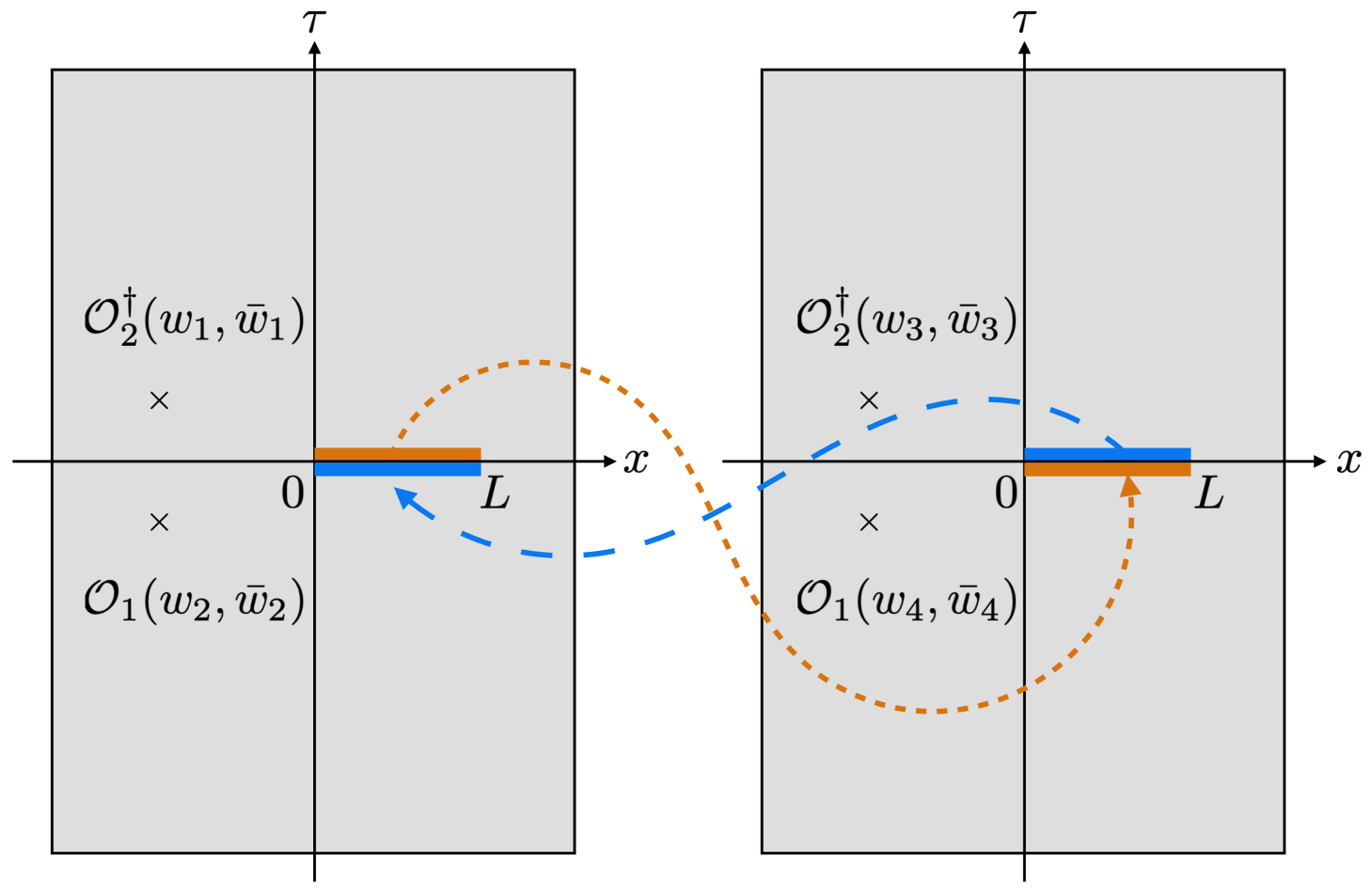
Figure 3: Euclidean path integral on $\Sigma_{2}$ for calculating the numerator of the correlation function in (28).

For further computation of the correlation function (28), we consider a conformal transformation from $\Sigma_{2}$ to $\Sigma_{1}$,

$$\frac{w}{w-L}=z^{2}.$$ (29)

In particular, each point $w_{i}\in\Sigma_{2}(i=1,\cdots,4)$ maps to $z_{i}\in\Sigma_{1}(i=1,\cdots,4)$ as follows

$$z_{1} =-z_{3}=\sqrt{(l-t-ia)/(l+L-t-ia)},$$ (30)

$$z_{2} =-z_{4}=\sqrt{(l-t+ia)/(l+L-t+ia)}.$$ (31)

Amplification of pseudo Rényi entropy

After straightforward calculation, we obtain

$$\frac{\braket{\mathcal{O}_{2}^{\dagger}(w_{1},\bar{w}_{1})\mathcal{O}_{1}(w_{2},\bar{w}_{2})\mathcal{O}_{2}^{\dagger}(w_{3},\bar{w}_{3})\mathcal{O}_{1}(w_{4},\bar{w}_{4})}_{\Sigma_{2}}}{(\braket{\mathcal{O}_{2}^{\dagger}(w_{1},\bar{w}_{1})\mathcal{O}_{1}(w_{2},\bar{w}_{2})}_{\Sigma_{1}})^{2}}=\frac{1}{2\epsilon^{2}}\left[(1+\epsilon^{2})-(1-\epsilon^{2})(|1-z|+|z|)\right],$$ (32)

where we introduced the cross ratio

$$z=\dfrac{(z_{1}-z_{2})(z_{3}-z_{4})}{(z_{1}-z_{3})(z_{2}-z_{4})}.$$ (33)

Under the time evolution with small $a$ limit, we have

$$(z,\bar{z})\rightarrow\begin{cases}(0,0)&(\text{$0<t<\ell$ or $\ell+L<t$}),\\ (1,0)&\qquad(\ell<t<\ell+L).\end{cases}$$ (34)

Therefore, we obtain

$$\Delta S^{(2)}(\tau_{A}^{\varphi|\psi})=\begin{cases}0&(\text{$0<t<\ell$ or $\ell+L<t$}),\\ \log\left(\frac{2\epsilon^{2}}{1+\epsilon^{2}}\right)&\qquad(\ell<t<\ell+L).\end{cases}$$ (35)

For $\ell<t<\ell+L$, one of the propagating EPR pairs (the right-moving particle) is in subsystem $A$, hence we obtain a non-trivial pseudo Rényi entropy. In particular, this exactly matches the previous result in section 2.

4 Non-amplification in Holographic CFT

Finally, we move on to the two-dimensional holographic CFTs, dual to three-dimensional Einstein gravity in AdS. We would like to consider a similar setup as the previous sections and see if the amplification occurs. For this, we discuss a specific linear combination of the so-called heavy states, microstates of the BTZ black hole [32],

$$\ket{\psi} =\ket{\mathcal{O}_{H_{1}}}+\epsilon\ket{\mathcal{O}_{H_{2}}},$$ (36)

$$\ket{\varphi} =\ket{\mathcal{O}_{H_{2}}},$$ (37)

where $\ket{\mathcal{O}_{H_{1}}}$ and $\ket{\mathcal{O}_{H_{2}}}$ are assumed to have different conformal dimensions $h_{H_{1}}$ and $h_{H_{2}}$. For simplicity, we consider the static black hole ($h_{H_{i}}=\bar{h}_{H_{i}}$). For being the heavy states, we assume $h_{H_{i}}/c\geq\frac{1}{24}$, where $c$ is the central charge. Since we assumed these heavy states have different conformal dimensions, they are orthogonal to each other,

$$\braket{\mathcal{O}_{H_{1}}}{\mathcal{O}_{H_{2}}}=0.$$ (38)

The conformal dimension $h$ and the radius of BTZ black hole $r_{+}$ are related as

$$r_{+}(h)=\sqrt{\frac{24}{c}h-1}.$$ (39)

The entanglement entropy of these heavy states $\rho^{(i)}=|\mathcal{O}_{H_{i}}\rangle\langle\mathcal{O}_{H_{i}}|$ with a small subsystem $A$ is computed as

$$S(\rho_{A}^{(i)})=\dfrac{c}{3}\log\left[\dfrac{2}{r_{+}(h_{H_{i}})\varepsilon_{\text{UV}}}\sinh\left(\dfrac{r_{+}(h_{H_{i}})\ell_{A}}{2}\right)\right]\;\;\;(i=1,2),$$ (40)

where $\varepsilon_{\text{UV}}$ is the UV cutoff and $\ell_{A}$ is the size of subsystem $A$. The central charge $c$ is given by the standard dictionary of AdS/CFT as $c=\frac{3}{2G_{N}}$, where $G_{N}$ is the three-dimensional Newton constant. One can confirm the above expression from both CFT [33]  and gravity analysis [6]. For sufficiently large black holes $r_{+}\gg 1$, the entanglement entropy (40) enjoys the volume law,

$$S(\rho_{A}^{(i)})\sim\dfrac{c}{3}\dfrac{\pi\ell_{A}}{\beta_{H_{i}}},$$ (41)

where $\beta_{H_{i}}=2\pi/r_{+}(h_{H_{i}})$ is the inverse temperature of BTZ black hole. Therefore, these states are quite similar to the previous Bell states: both states are highly entangled, but orthogonal to each other.

Let us compute the pseudo entropy for (36) and (37). The holographic pseudo entropy is computed as

$$S(\tau^{\psi|\varphi}_{A})=\dfrac{c}{3}\log\left[\dfrac{2}{r_{+}(h_{H_{2}})\varepsilon_{\text{UV}}}\sinh\left(\dfrac{r_{+}(h_{H_{2}})\ell_{A}}{2}\right)\right],$$ (42)

because the inner product of two states reduces to the one of the second heavy state,

$$\braket{\varphi}{\psi}=\epsilon\braket{\mathcal{O}_{H_{2}}}{\mathcal{O}_{H_{2}}}.$$ (43)

Notice that we have no $\epsilon$-parameter in the above expression (42). This is also consistent with one of the expected property of holographic pseudo entropy as the weak value of area operator [14],

$$S(\tau^{\psi|\varphi}_{A})=\dfrac{\braket{\varphi}{\frac{\hat{A}}{4G_{N}}}{\psi}}{\braket{\varphi}{\psi}}.$$ (44)

One can also confirm the above results from CFT analysis as [14]. Thus, we conclude that there is no amplification of pseudo entropy in this holographic example.

However, we have to stress that the discussion so far is true only when we can regard entanglement entropy/pseudo entropy as the expectation value/weak value of the area operator. This should not be always true because the modular Hamiltonian is state-dependent and non-linear with respect to the states. In particular, for non-amplification, heavy states should be eigenstates of the area operator or reduced density/transition matrix.

Saying differently, we expect that the area operator also has exponentially small off-diagonal elements as discussed in [36]. A schematic understanding is as follows. If we assume the eigenstate thermalization hypothesis (ETH) [37, 38, 39] like relation for the area operator, we have

$$\langle E_{i}|\hat{A}|E_{j}\rangle=A(E)\delta_{ij}+\mathrm{e}^{-S(E)/2}g_{\mathcal{A}}(E_{i},E_{j})R_{ij},$$ (45)

where the diagonal element $A(E)$ is the thermal expectation value, $S(E)$ is the entropy at energy $E=(E_{i}+E_{j})/2$,  $g_{\mathcal{A}}(E_{i},E_{j})$ is $\mathcal{O}(1)$ function and $R_{ij}$ is the random matrix with unit variance. The point here is that the second (off-diagonal) term is exponentially suppressed for the entropy which is of order $S=\mathcal{O}(c)$. In our case, since the heavy states are the energy eigenstates of the CFT Hamiltonian, we schematically obtain

$$\dfrac{\langle{\varphi}|\frac{\hat{A}}{4G_{N}}|{\psi}\rangle}{\langle{\varphi}|{\psi}\rangle}=S(\rho^{(2)}_{A})+\frac{1}{\epsilon}\mathrm{e}^{-\mathcal{O}(c)}(\textrm{off-diagonal part}).$$ (46)

Therefore, if we take $\epsilon$ as small as $e^{-\mathcal{O}(c)}$, we can no longer neglect the second term (46) and we will see the amplification.

5 Discussion

In this paper, we have studied pseudo entropy for the particular type of linear combination in various setups and discuss when the (non-)amplification happens. In particular, the linear combination of the heavy states in holographic CFT does not give rise to amplification as long as the overlap $\braket{\varphi}{\psi}$ is much larger than $e^{-\mathcal{O}(c)}$.

An immediate but interesting future direction is to study if there are any field theoretic setups other than the holographic CFT where the amplification does not happen. It might serve as a sharp criterion whether a given QFT is in a “holographic regime”. Another obvious future task is to generalize field theory results to higher dimensions. Assuming the Lewkowycz-Maldacena type argument [8], the generalization of our holographic results to the higher dimension is straightforward, but the full understanding of the validity regime requires non-perturbative treatment. For this, it would be instructive to utilize so-called fixed area states or random tensor networks [40, 41, 42, 43, 44, 45, 46].

We used a very specific linear combination to compare the results for different systems. This linear combination is ideal but appears to be artificial for amplification. One of the most interesting situations for amplification is when two states belong to different quantum phases [16, 17, 18]. In these situations, one can see

$$\Delta S(\tau_{A}^{\psi|\varphi})\equiv\dfrac{1}{2}\left[S(\tau_{A}^{\psi|\varphi})+S(\tau_{A}^{\psi|\varphi})^{\ast}-S(\tau_{A}^{\psi|\psi})-S(\tau_{A}^{\varphi|\varphi})\right]>0,$$ (47)

which implies the amplification discussed in this paper. It would be intriguing to study our setup from the viewpoint of the energy eigenstates of gapped Hamiltonians. It is also interesting to construct explicit gravity solutions that show $\Delta S(\tau_{A}^{\psi|\varphi})>0$.

Since the Rényi entropy can be observed in the lab [47], it is a very important future problem to design measurement for the pseudo Rényi entropy in the real experiment. We leave these interesting directions for further work.

References

- [1] M. A. Nielsen and I. Chuang, Quantum computation and quantum information. American Association of Physics Teachers, 2002.
- [2] G. Vidal, J. I. Latorre, E. Rico and A. Kitaev, Entanglement in quantum critical phenomena, Phys. Rev. Lett. 90 (2003) 227902 [quant-ph/0211074].
- [3] P. Calabrese and J. L. Cardy, Entanglement entropy and quantum field theory, J. Stat. Mech. 0406 (2004) P06002 [hep-th/0405152].
- [4] A. Kitaev and J. Preskill, Topological entanglement entropy, Phys. Rev. Lett. 96 (2006) 110404 [hep-th/0510092].
- [5] M. Levin and X.-G. Wen, Detecting Topological Order in a Ground State Wave Function, Phys. Rev. Lett. 96 (2006) 110405 [cond-mat/0510613].
- [6] S. Ryu and T. Takayanagi, Holographic derivation of entanglement entropy from AdS/CFT, Phys. Rev. Lett. 96 (2006) 181602 [hep-th/0603001].
- [7] V. E. Hubeny, M. Rangamani and T. Takayanagi, A Covariant holographic entanglement entropy proposal, JHEP 07 (2007) 062 [0705.0016].
- [8] A. Lewkowycz and J. Maldacena, Generalized gravitational entropy, JHEP 08 (2013) 090 [1304.4926].
- [9] J. M. Maldacena, Eternal black holes in anti-de Sitter, JHEP 04 (2003) 021 [hep-th/0106112].
- [10] B. Swingle, Entanglement Renormalization and Holography, Phys. Rev. D 86 (2012) 065007 [0905.1317].
- [11] M. Van Raamsdonk, Comments on quantum gravity and entanglement, 0907.2939.
- [12] M. Van Raamsdonk, Building up spacetime with quantum entanglement, Gen. Rel. Grav. 42 (2010) 2323 [1005.3035].
- [13] F. Pastawski, B. Yoshida, D. Harlow and J. Preskill, Holographic quantum error-correcting codes: Toy models for the bulk/boundary correspondence, JHEP 06 (2015) 149 [1503.06237].
- [14] Y. Nakata, T. Takayanagi, Y. Taki, K. Tamaoka and Z. Wei, New holographic generalization of entanglement entropy, Phys. Rev. D 103 (2021) 026005 [2005.13801].
- [15] I. Akal, T. Kawamoto, S.-M. Ruan, T. Takayanagi and Z. Wei, On the Page curve under final state projection, 2112.08433.
- [16] A. Mollabashi, N. Shiba, T. Takayanagi, K. Tamaoka and Z. Wei, Pseudo Entropy in Free Quantum Field Theories, Phys. Rev. Lett. 126 (2021) 081601 [2011.09648].
- [17] A. Mollabashi, N. Shiba, T. Takayanagi, K. Tamaoka and Z. Wei, Aspects of pseudoentropy in field theories, Phys. Rev. Res. 3 (2021) 033254 [2106.03118].
- [18] T. Nishioka, T. Takayanagi and Y. Taki, Topological pseudo entropy, JHEP 09 (2021) 015 [2107.01797].
- [19] P.-Y. Chang, J.-S. You, X. Wen and S. Ryu, Entanglement spectrum and entropy in topological non-Hermitian systems and nonunitary conformal field theory, Phys. Rev. Res. 2 (2020) 033069 [1909.01346].
- [20] K. Goto, M. Nozaki and K. Tamaoka, Subregion spectrum form factor via pseudoentropy, Phys. Rev. D 104 (2021) L121902 [2109.00372].
- [21] M. Miyaji, Island for gravitationally prepared state and pseudo entanglement wedge, JHEP 12 (2021) 013 [2109.03830].
- [22] G. Camilo and A. Prudenziati, Twist operators and pseudo entropies in two-dimensional momentum space, 2101.02093.
- [23] S. Murciano, P. Calabrese and R. M. Konik, Generalized entanglement entropies in two-dimensional conformal field theory, JHEP 05 (2022) 152 [2112.09000].
- [24] J. Mukherjee, Pseudo Entropy in gauge theory, 2205.08179.
- [25] W.-z. Guo, S. He and Y.-X. Zhang, On the real-time evolution of pseudo-entropy in 2d CFTs, 2206.11818.
- [26] Y. Aharonov, D. Z. Albert and L. Vaidman, How the result of a measurement of a component of the spin of a spin-1/2 particle can turn out to be 100, Phys. Rev. Lett. 60 (1988) 1351.
- [27] J. Dressel, M. Malik, F. M. Miatto, A. N. Jordan and R. W. Boyd, Colloquium: Understanding quantum weak values: Basics and applications, Reviews of Modern Physics 86 (2014) 307.
- [28] M. Nozaki, T. Numasawa and T. Takayanagi, Quantum Entanglement of Local Operators in Conformal Field Theories, Phys. Rev. Lett. 112 (2014) 111602 [1401.0539].
- [29] M. Nozaki, Notes on Quantum Entanglement of Local Operators, JHEP 10 (2014) 147 [1405.5875].
- [30] P. Caputa, M. Nozaki and T. Takayanagi, Entanglement of local operators in large-N conformal field theories, PTEP 2014 (2014) 093B06 [1405.5946].
- [31] S. He, T. Numasawa, T. Takayanagi and K. Watanabe, Quantum dimension as entanglement entropy in two dimensional conformal field theories, Phys. Rev. D 90 (2014) 041701 [1403.0702].
- [32] M. Banados, C. Teitelboim and J. Zanelli, The Black hole in three-dimensional space-time, Phys. Rev. Lett. 69 (1992) 1849 [hep-th/9204099].
- [33] C. T. Asplund, A. Bernamonti, F. Galli and T. Hartman, Holographic Entanglement Entropy from 2d CFT: Heavy States and Local Quenches, JHEP 02 (2015) 171 [1410.1392].
- [34] Y. Kusuki and K. Tamaoka, Dynamics of Entanglement Wedge Cross Section from Conformal Field Theories, Phys. Lett. B 814 (2021) 136105 [1907.06646].
- [35] Y. Kusuki and K. Tamaoka, Entanglement Wedge Cross Section from CFT: Dynamics of Local Operator Quench, JHEP 02 (2020) 017 [1909.06790].
- [36] A. Almheiri, X. Dong and B. Swingle, Linearity of Holographic Entanglement Entropy, JHEP 02 (2017) 074 [1606.04537].
- [37] M. Srednicki, The approach to thermal equilibrium in quantized chaotic systems, Journal of Physics A: Mathematical and General 32 (1999) 1163.
- [38] L. D’Alessio, Y. Kafri, A. Polkovnikov and M. Rigol, From quantum chaos and eigenstate thermalization to statistical mechanics and thermodynamics, Adv. Phys. 65 (2016) 239 [1509.06411].
- [39] R. Mondaini and M. Rigol, Eigenstate thermalization in the two-dimensional transverse field ising model. ii. off-diagonal matrix elements of observables, Physical Review E 96 (2017) .
- [40] C. Akers and P. Rath, Holographic Renyi Entropy from Quantum Error Correction, JHEP 05 (2019) 052 [1811.05171].
- [41] X. Dong, D. Harlow and D. Marolf, Flat entanglement spectra in fixed-area states of quantum gravity, JHEP 10 (2019) 240 [1811.05382].
- [42] N. Bao, G. Penington, J. Sorce and A. C. Wall, Beyond Toy Models: Distilling Tensor Networks in Full AdS/CFT, JHEP 11 (2019) 069 [1812.01171].
- [43] N. Bao, G. Penington, J. Sorce and A. C. Wall, Holographic Tensor Networks in Full AdS/CFT, 1902.10157.
- [44] P. Hayden, S. Nezami, X.-L. Qi, N. Thomas, M. Walter and Z. Yang, Holographic duality from random tensor networks, JHEP 11 (2016) 009 [1601.01694].
- [45] G. Penington, S. H. Shenker, D. Stanford and Z. Yang, Replica wormholes and the black hole interior, JHEP 03 (2022) 205 [1911.11977].
- [46] C. Akers and G. Penington, Leading order corrections to the quantum extremal surface prescription, JHEP 04 (2021) 062 [2008.03319].
- [47] R. Islam, R. Ma, P. M. Preiss, M. E. Tai, A. Lukin, M. Rispoli et al., Measuring entanglement entropy through the interference of quantum many-body twins, 1509.01160.