Revisiting Label Smoothing and Knowledge Distillation Compatibility
What was Missing?

Abstract

This work investigates the compatibility between label smoothing (LS) and knowledge distillation (KD). Contemporary findings addressing this thesis statement take dichotomous standpoints: Müller et al. (2019); Shen et al. (2021b). Critically, there is no effort to understand and resolve these contradictory findings, leaving the primal question $-$ to smooth or not to smooth a teacher network? $-$ unanswered. The main contributions of our work are the discovery, analysis and validation of systematic diffusion as the missing concept which is instrumental in understanding and resolving these contradictory findings. This systematic diffusion essentially curtails the benefits of distilling from an LS-trained teacher, thereby rendering KD at increased temperatures ineffective. Our discovery is comprehensively supported by large-scale experiments, analyses and case studies including image classification, neural machine translation and compact student distillation tasks spanning across multiple datasets and teacher-student architectures. Based on our analysis, we suggest practitioners to use an LS-trained teacher with a low-temperature transfer to achieve high performance students. Code and models are available at https://keshik6.github.io/revisiting-ls-kd-compatibility/

1 Introduction

This paper deeply investigates the compatibility between label smoothing (Szegedy et al., 2016) and knowledge distillation (Hinton et al., 2015). Specifically, we aim to revisit and resolve the contradictory standpoints of Müller et al. (2019) and Shen et al. (2021b), thereby establishing a foundational understanding on the compatibility between label smoothing (LS) and knowledge distillation (KD). Both LS and KD involve training a model (i.e.: deep neural networks) with soft-targets. In LS, instead of computing cross entropy loss with the hard-target (one-hot encoding) of a training sample, a soft-target is used, which is a weighted mixture of the one-hot encoding and the uniform distribution. A mixture parameter $\alpha$ is used in LS to specify the extent of mixing. On the other hand, KD involves training a teacher model (usually a powerful model) and a student model (usually a compact model). The objective of KD is to transfer knowledge from the teacher model to the student model. In the most common form, the student model is trained to match the soft output of the teacher model. The success of KD has been attributed to the transference of logits’ information about resemblances between instances of different classes (logits are the inputs to the final softmax which produces the soft targets). In KD (Hinton et al., 2015), a temperature $T$ is introduced to facilitate the transference: an increased $T$ may produce more suitable soft targets that have more emphasis on the probabilities of incorrect classes (or equivalently, logits of the incorrect classes).

LS and KD research dialogue. Recently, a notable amount of research efforts has been conducted to understand the relationship between LS and KD (Müller et al., 2019; Shen et al., 2021b; Lukasik et al., 2020; Yuan et al., 2020; Tang et al., 2021). One of the most intriguing and controversial discussion is the compatibility between LS and KD. Particularly, in KD, does label smoothing in a teacher network suppress the effectiveness of the distillation?

Müller et al. (2019) are the first to investigate this topic, and their findings suggest that applying LS to a teacher network impairs the performance of KD. In particular, they visualize the penultimate layer representations in the teacher network to show that LS erases information in the logits about resemblances between instances of different classes. Since this information is essential for KD, they conclude that applying LS for the teacher network can hurt KD. $\bullet$ “If a teacher network is trained with label smoothing, knowledge distillation into a student network is much less effective.” (Müller et al., 2019) $\bullet$ “Label smoothing can hurt distillation” (Müller et al., 2019)

The conclusion of Müller et al. (2019) is widely accepted (Khosla et al., 2020; Arani et al., 2021; Tang et al., 2021; Mghabbar & Ratnamogan, 2020; Shen et al., 2021a). However, very recently, this is questioned by Shen et al. (2021b). In particular, their work discussed a new finding: information erasure in teacher can actually enlarge the central distance between semantically similar classes, allowing the student to learn to classify these categories easily. Shen et al. (2021b) claim that this benefit of using an LS-trained teacher outweighs the detrimental effect due to information erasure. Therefore, they conclude that LS in a teacher network does not suppress the effectiveness of KD. $\bullet$ “Label smoothing will not impair the predictive performance of students.” (Shen et al., 2021b) $\bullet$ “Label smoothing is compatible with knowledge distillation” (Shen et al., 2021b)

LS and KD compatibility remains unresolved. We were perplexed by the seemingly contradictory findings by Müller et al. (2019) and Shen et al. (2021b). While the latter has shown empirical results to support their own finding, their work does not investigate the opposite standpoint and contradictory results by Müller et al. (2019). Critically, there is no effort to understand and resolve the seemingly contradictory arguments and supporting evidences by Müller et al. (2019) and Shen et al. (2021b). Consequently, for practitioners, it remains unclear as to under what situations LS can be applied to the teacher network in KD, and under what situations it must be avoided.

Our contributions. We begin by meticulously scrutinizing the opposing findings of Müller et al. (2019) and Shen et al. (2021b). In particular, we discover that in the presence of an LS-trained teacher, KD at higher temperatures systematically diffuses penultimate layer representations learnt by the student towards semantically similar classes. This systematic diffusion essentially curtails the benefits (as claimed by Shen et al. (2021b)) obtained by distilling from an LS-trained teacher, thereby rendering KD at increased temperatures ineffective. We perform large-scale KD experiments including image classification using ImageNet-1K (Deng et al., 2009), fine-grained image classification using CUB200-2011 (Wah et al., 2011), neural machine translation (English $\rightarrow$ German, English $\rightarrow$ Russian translation) using IWSLT, compact student distillation (MobileNetV2 (Sandler et al., 2018), EfficientNet-B0 (Tan & Le, 2019)) and multiple teacher-student architectures to comprehensively demonstrate this systematic diffusion in the student qualitatively using penultimate layer visualizations, and quantitatively using our proposed relative distance metric called diffusion index ($\eta$).

Our finding on systematic diffusion is very critical when distilling from an LS-trained teacher. Particularly, we argue that this diffusion maneuvers the penultimate layer representations learnt by the student of a given class in a systematic way that targets in the direction of semantically similar classes. Therefore, this systematic diffusion directly curtails the distance enlargement (between semantically similar classes) benefits obtained by distilling from an LS-trained teacher. Our qualitative and quantitative analysis with our proposed relative distance metric ($\eta$) in Sec. 4 aims to establish not only the existence of this diffusion, but also establish that such diffusion is systematic and not isotopic.

Importantly, using systematic diffusion analysis, we explain and resolve the contradictory findings by Müller et al. (2019) and Shen et al. (2021b), thereby establishing a foundational understanding on the compatibility between LS and KD. Finally, using our discovery on systematic diffusion, we provide empirical guidelines for practitioners regarding the combined use of LS and KD. We summarize our key findings in Table 1. The key takeaway from our work is:

• In the presence of an LS-trained teacher, KD at higher temperatures systematically diffuses penultimate layer representations learnt by the student towards semantically similar classes. This systematic diffusion essentially curtails the benefits of distilling from an LS-trained teacher, thereby rendering KD at increased temperatures ineffective. Specifically, systematic diffusion was the missing concept that is instrumental in explaining and resolving the contradictory findings of Müller et al. (2019) and Shen et al. (2021b), thereby clearing up the existential conundrum regarding the compatibility between LS and KD.

Table 1: Main findings regarding LS and KD compatibility in recent works and our work.

Information
erasure
(incompatibility) Distance
enlargement
(compatibility) Our main finding:
Systematic diffusion
(incompatibility) Conclusion Müller et al. (2019) LS erases relative information in the logits LS-trained teacher can hurt KD Shen et al. (2021b) With LS, some relative information in the logits is still retained LS enlarges the distance between semantically similar classes Benefits outweigh disadvantages. LS is compatible with KD Our work Lower $T$ ($i.e.:T=1$) We agree with (Shen et al., 2021b) in information erasure We experimentally validate the inheritance of distance enlargement in the student, see Figure 1. (Shen et al. (2021b) has not shown this). With KD of lower $T$ (i.e.: $T$=1), there is lower degree of systematic diffusion of penultimate representations towards semantically similar classes. This doesn’t curtail the distance enlargement benefit. At lower levels of systematic diffusion in student. LS is compatible with KD Increase of $T$ The loss of logits’ relative information cannot be recovered with an increased $T$ We agree with (Shen et al., 2021b) observation, but the distance enlargement is curtailed at an increased $T$. With KD of increased $T$, there is systematic diffusion of penultimate representations towards semantically similar classes, curtailing the distance enlargement (Sec. 4). At higher levels of systematic diffusion in student. LS and KD are not compatible.

A rule of thumb for practitioners. We suggest to use an LS-trained teacher with a low-temperature transfer (i.e. $T$ = 1) to achieve high performance students.

Paper organization. In Sec. 2, we review LS and KD. In Sec. 3, we revisit key findings of (Müller et al., 2019) and Shen et al. (2021b) to emphasize the research gap. Our main contribution is Sec. 4, where we introduce our discovered systematic diffusion, conduct qualitative, quantitative and analytical studies to verify that the diffusion is not isotopic but systematic towards semantically-similar classes, and therefore it directly curtails the benefits of using an LS-trained teacher. In Sec. 5, we perform rich empirical studies to support our main finding on Systematic Diffusion. In Sec. 6 , we conduct extended experiments using compact students and neural machine translation tasks to further support our finding. In Sec. 7, we provide our perspective regarding the combined use of LS and KD as empirical guidelines for practitioners, and finally conclude this study.

2 Prerequisites

Label Smoothing (LS) (Szegedy et al., 2016): LS was formulated as a regularization strategy to alleviate models’ over-confidence. LS replaces the original hard target distribution with a mixture of original hard target distribution and the uniform distribution characterized by the mixture parameter $\alpha$. Many state-of-the-art models have leveraged on LS to improve the accuracy of deep neural networks across multiple tasks including image classification (He et al., 2019; Real et al., 2019; Zoph et al., 2018; Huang et al., 2019), machine translation (Vaswani et al., 2017) and speech recognition (Chorowski & Jaitly, 2017; Chiu et al., 2018; Pereyra et al., 2017). Consider the formulation of LS objective with mixture parameter $\alpha$ as follows: Let $p_{k},\mathbf{w}_{k}$ represent the probability and last layer weights (including biases) corresponding to the $k$-th class. Let $\mathbf{x},y_{k},y_{k}^{LS}$ represent the penultimate layer activations, true targets and LS-targets where $y_{k}=1$ for the correct class and 0 for all the incorrect classes. $\mathbf{x}^{T}$ is the transpose of $\mathbf{x}$. Then for a classification network trained with LS containing $K$ classes, we minimize the cross entropy loss between LS-targets $y_{k}^{LS}$ and model predictions $p_{k}$ given by $L_{LS}(\mathbf{y},\mathbf{p})=\sum_{k=1}^{K}-y_{k}^{LS}\log(p_{k})$, where $p_{k}={\exp({\mathbf{x}^{T}\mathbf{w}_{k}})}/{\sum_{l=1}^{K}\exp({\mathbf{x}^{T}\mathbf{w}_{l}})}$ and $y_{k}^{LS}=y_{k}(1-\alpha)+\frac{\alpha}{K}$.

Knowledge distillation (KD) Hinton et al. (2015): KD uses a larger capacity teacher model(s) to transfer the knowledge to a compact student model. Recently KD methods have been widely used in visual recognition (Zhang et al., 2020; Peng et al., 2019; Lopez-Paz et al., 2016), NLP (Hu et al., 2018; Jiao et al., 2020; Nakashole & Flauger, 2017) and speech recognition (Shen et al., 2020; Kwon et al., 2020; Perez et al., 2020). The success of KD methods is largely attributed to the information about incorrect classes encoded in the output distribution produced by the teacher model(s) (Hinton et al., 2015). Consider KD for a classification objective. Let $T$ indicate the temperature factor that controls the importance of each soft target. Given the $k$-th class logit $\mathbf{x}^{T}\mathbf{w}_{k}$, let the temperature scaled probability be $p_{k}(T)$. For KD training, let the loss be $L_{KD}$. For $L_{KD}$, we replace the cross entropy loss $H(\mathbf{y},\mathbf{p})$ with a weighted sum (parametrized by $\beta$) of $H(\mathbf{y},\mathbf{p})$ and $H(\mathbf{p}^{t}(T),\mathbf{p}(T))$ where $\mathbf{p}^{t}(T),\mathbf{p}(T)$ correspond to the temperature-scaled teacher and student output probabilities. That is, $p_{k}(T)={\exp(\frac{{\mathbf{x}^{T}\mathbf{w}_{k}}}{T})}/{\sum_{l=1}^{K}\exp(\frac{\mathbf{x}^{T}\mathbf{w}_{l}}{T})}$ and $L_{KD}=(1-\beta)H(\mathbf{y},\mathbf{p})+\beta T^{2}H(\mathbf{p}^{t}(T),\mathbf{p}(T))$. Following Hinton et al. (2015) $T^{2}$ scaling is used for the soft-target optimization as $T$ will scale the gradients approximately by a factor of $1/T^{2}$. Following Müller et al. (2019); Shen et al. (2021b), we set $\beta=1$ for this study since we primarily aim to isolate and study the effects of KD. $\beta=1$ achieves good performance (Shen et al., 2021b).

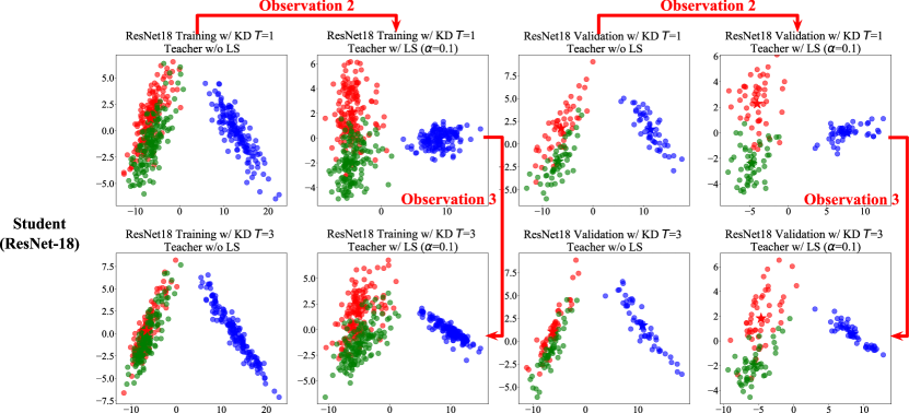
Figure 1: Visualization of the penultimate layer representations (Teacher = ResNet-50, Student = ResNet-18, Dataset = ImageNet). We follow the same setup and procedure used in Müller et al. (2019) and Shen et al. (2021b). We also follow their three-class analysis: two semantically similar classes ( miniature_poodle, standard_poodle) and one semantically different class ( submarine). Additional visualization can be found in the Supplementary. Observation 1: The use of LS on the teacher leads to tighter clusters and erasure of logits’ information as claimed by Müller et al. (2019). In addition, increase in central distance between semantically similar classes ( miniature_poodle, standard_poodle) as claimed by Shen et al. (2021b) can be observed. Observation 2: We further visualize the student’s representations. Increase in central distance between semantically similar classes can also be observed. This confirms the transfer of this benefit from the teacher to the student. Note that in Müller et al. (2019) and Shen et al. (2021b), student’s representations have not been visualized. Observation 3 (Our main discovery): KD of an increased $T$ causes systematic diffusion of representations between semantically similar classes ( miniature_poodle, standard_poodle). This curtails the increment of central distance between semantically similar classes due to the use of LS-trained teacher. We notice similar observations in other datasets and networks, see Figures A.1, A.3, A.4, A.2 and A.5. We also include image samples for these 3 classes in Supplementary Figure L.1. Best viewed in color.

3 A Closer Look at LS and KD compatibility

In this section, we review the contradictory findings of Müller et al. (2019) and Shen et al. (2021b) from the perspective of information erasure in LS-trained teacher. This discussion is a necessary preamble to understand our main finding, Systematic Diffusion in the student in Sec. 4.

Information erasure in LS-trained teacher. LS objective optimizes the probability of the correct class to be equal to $1-\alpha$ + $\alpha/K$, and incorrect classes to be $\alpha/K$. This directly encourages the differences between logits of the correct class and incorrect classes to be a constant (Müller et al., 2019) determined by $\alpha$. Following Müller et al. (2019), the logit $\mathbf{x}^{T}\mathbf{w}_{k}$ can be approximately measured using the squared Euclidean distance between penultimate layer’s activations and the template corresponding to class $k$. That is, $\mathbf{x}^{T}\mathbf{w}_{k}$ can be approximately measured by $\|{\mathbf{x}-\mathbf{w}_{k}}\|^{2}$. This allows to establish 2 important geometric properties of LS (Müller et al., 2019): With LS, penultimate layer activations 1) are encouraged to be close to the template of the correct class (large logit value for the correct class, therefore small distance between the activations and the correct class template), and 2) are encouraged to be equidistant to the templates of the incorrect classes (equal logit values for all the incorrect classes). This results in penultimate layer activations to tightly cluster around the correct class template compared to the model trained with standard cross entropy objective. We demonstrate this clearly in Figure 1 Observation 1. With LS applied on the ResNet-50 model, we observe that the penultimate layer representations become much tighter. As a result, substantial information regarding the resemblances of these instances to those of other different classes is lost. This is referred to as the information erasure in LS-trained teacher (Müller et al., 2019).

Müller et al. (2019) finding: Information erasure in LS-trained teacher cause LS and KD to be Incompatible: Müller et al. (2019) are the first to investigate this compatibility, and they argue that the information erasure effect due to LS (shown in Figure 1 Observation 1) can impair KD. Given the prominent successes in KD methods being largely attributed to dark knowledge/ inter-class information emerging from the trained-teacher (Hinton et al., 2015; Tang et al., 2021), the argument by Müller et al. (2019) that LS and KD are incompatible due to information loss in the logits is generally convincing and widely accepted (Khosla et al., 2020; Arani et al., 2021; Tang et al., 2021; Mghabbar & Ratnamogan, 2020; Shen et al., 2021a). This is also supported by empirical evidence.

Shen et al. (2021b) finding: Information erasure in LS-trained teacher provides distance enlargement benefits between semantically similar classes, resulting in LS and KD to be Compatible: Recently an interesting finding by Shen et al. (2021b) argue that LS and KD are compatible. Though they agree that information erasure generally happens with LS, their argument focuses more on the effect of LS on semantically similar classes. They argue that information erasure in LS-trained teacher can promote enlargement of central distance of clusters between semantically similar classes. This allows the student network to easily learn to classify semantically similar classes which are generally difficult to classify in conventional training procedures. We show this increased separation between semantically similar classes with LS in Figure 1 Observation 1. It can be observed that the central distance between the clusters of standard_poodle and miniature_poodle increases with using LS on the ResNet-50 teacher. In our work, we further extend to show that this property is inherited by the ResNet-18 student as well in Observation 2. We remark that this inheritance is not shown by Shen et al. (2021b). This finding by Shen et al. (2021b) is supported by experiments and quantitative results. Though they claim that the benefit derived from larger separation between semantically similar classes outweigh the drawbacks due to information erasure, thereby making LS and KD compatible, their investigation does not address the contradictory findings and results reported by Müller et al. (2019).

Research Gap: Studied in isolation, both these contradictory arguments are convincing and well supported empirically. This has caused serious perplexity among the research community regarding the combined use of LS and KD.

4 Systematic Diffusion in Student

Through profound investigation, we discover an intriguing phenomenon occurring in the student called systematic diffusion when distilling from an LS-trained teacher at higher $T$. Particularly, this diffusion maneuvers the penultimate layer representations learnt by the student of a given class in a systematic way that targets in the direction of semantically similar classes. This systematic diffusion is critical as it directly curtails the distance enlargement benefits between semantically similar classes when distilling from an LS-trained teacher.

Penultimate layer visualization as evidence of systematic diffusion. We follow Müller et al. (2019), and use their visualization method based on linear projections of the penultimate layer representations. See Figure 1 for visualization (We discuss Figure 1 deeply in Sec. 5). Particularly, our discovery on systematic diffusion affects the distance between semantically similar classes in the student when distilled from an LS-trained teacher at higher $T$. This systematic diffusion can be clearly observed by visualizing the penultimate layer representations of the student. We include the visualization algorithm and Numpy-style code in Supplementary F.

Given that the increased cluster center separation between semantically similar classes being the reason for the compatibility claim between LS and KD (Shen et al., 2021b), we discover that this cluster center separation is affected by the degree of systematic diffusion in the student. Importantly, systematic diffusion is instrumental in explaining and resolving the contradictory findings of Müller et al. (2019) and Shen et al. (2021b), thereby establishing a foundational understanding on the compatibility between LS and KD.

Formulation of Diffusion index ($\eta$) to measure systematic diffusion. To comprehensively support our discovery, we formulate a novel metric called diffusion index ($\eta$) to quantitatively measure this systematic diffusion. Given that the interpretation of ‘semantics’ is rather subjective, we carefully construct this metric to support our discovery. The basic idea of this metric is to quantify the distance change between clusters in the student network when distilled from an LS-trained teacher at higher $T$. Critically, the design of the metric is to verify that the diffusion is systematic: i.e. at higher $T$, inter-cluster distance decreases for semantic similar classes and increases (relatively) for the remaining classes. As explained in the Introduction, this systematic behaviour is critical in our study. There are important considerations in formulating this metric discussed below.

• A target class $\pi$ can be characterized by the centroid of the penultimate layer representations of samples belonging to $\pi$. Let the centroid of class $\pi$ be $c_{\pi}$.

• Consider the sets $S_{1},S_{2}$ where $S_{1}$ contains $|S_{1}|$ semantically similar classes to $\pi$ and $S_{2}$ contains $|S_{2}|$ semantically dissimilar classes to $\pi$. $|S|$ indicates the number classes in the set $S$. For easier understanding, consider 2 classes $p,q$ where $p\in S_{1},q\in S_{2}$.

• The proximity of $c_{\pi}$ to $c_{p}$ can approximately measure the semantic similarity between class $\pi$ and $p$. Though this proximity can be directly measured by Euclidean distance between centroids, it requires some careful thought on normalization. The reason is as follows: What we are interested is how close is centroid of class $\pi$ to class $p$ compared to class $q$. In other words, we are interested in the relative distance between centroids of classes $(\pi,p)$ and $(\pi,q)$. Hence to measure this relative distance we normalize the distance by the sum of pairwise distance from $c_{\pi}$ to centroids of all other classes in $S$.

• Do note that the location of the centroids will change with temperature. In fact, we are interested in the change of centroids with increased $T$ to measure this systematic diffusion. We formulate the following diffusion index $\eta$ to measure the average percentage change in distances between semantically similar classes and semantically dissimilar classes with respect to a target class.

Given a class $\pi$ and its centroid $\mathbf{c}_{\pi}$. Let the centroid of a class $k$ be represented by $\mathbf{c}_{k}$, $k\in{S_{1},S_{2}}$. Let the temperature be $T$. We quantify the relative distance between classes $\pi$ and $k$:

$d(\mathbf{c}_{\pi}(T),\mathbf{c}_{k}(T))=\frac{\|\mathbf{c}_{\pi}(T)-\mathbf{c}_{k}(T)\|^{2}}{R}$, where $R=\sum_{p\in S_{1}}\|\mathbf{c}_{\pi}(T)-\mathbf{c}_{p}(T)\|^{2}+\sum_{q\in S_{2}}\|\mathbf{c}_{\pi}(T)-\mathbf{c}_{q}(T)\|^{2}$ (normalization constant). The diffusion index $\eta$ measures the average percentage change in distance between a target class $\pi$ and classes in the set $S$ when temperature is changed from $T_{1}$ to $T_{2}$ defined as follows:

$$\eta(T_{1},T_{2};\pi,S)=\frac{1}{|S|}\sum_{k\in S}\frac{\delta}{d(\mathbf{c}_{\pi}(T_{1}),\mathbf{c}_{k}(T_{1}))},$$ (1)

where $\delta=d(\mathbf{c}_{\pi}(T_{2}),\mathbf{c}_{k}(T_{2}))-d(\mathbf{c}_{\pi}(T_{1}),\mathbf{c}_{k}(T_{1}))$. Substituting $S_{1}$, $S_{2}$ into $S$ of Eq. 1, we have: i) $\eta(T_{1},T_{2};\pi,S_{1})$ measures the change in relative distance between class $\pi$ and its semantically similar class in $S_{1}$. ii) $\eta(T_{1},T_{2};\pi,S_{2})$ measures the change in relative distance between class $\pi$ and its semantically dissimilar class in $S_{2}$. We discuss empirical results for $\eta$ in Sec. 5

To give more intuition on $\eta$, consider the 3 class example (Figure 1): miniature_poodle (as $\pi$ class), standard_poodle (as $p\in S_{1}$ and $|S_{1}|=1$), submarine (as $q\in S_{2}$ and $|S_{2}|=1$). As $T$ increases from $T_{1}=1$ to $T_{2}=3$, the relative distance between miniature_poodle and standard_poodle reduces due to diffusion (Figure 1), therefore $d(\mathbf{c}_{\pi}(T_{2}),\mathbf{c}_{p}(T_{2}))<d(\mathbf{c}_{\pi}(T_{1}),\mathbf{c}_{p}(T_{1}))$. From Eq. 1, it is clear that the numerator will be negative. We normalize by the reference distance to calculate the percentage change. As a result, the average percentage change over $S_{1}$ will be negative, indicating diffusion towards semantically similar classes. Similarly when measured over $S_{2}$, the average percentage change between miniature_poodle and submarine will be positive (because $d(\mathbf{c}_{\pi}(T_{2}),\mathbf{c}_{q}(T_{2}))>d(\mathbf{c}_{\pi}(T_{1}),\mathbf{c}_{q}(T_{1}))$ as observed in Figure 1) indicating diffusion away from $\pi$.

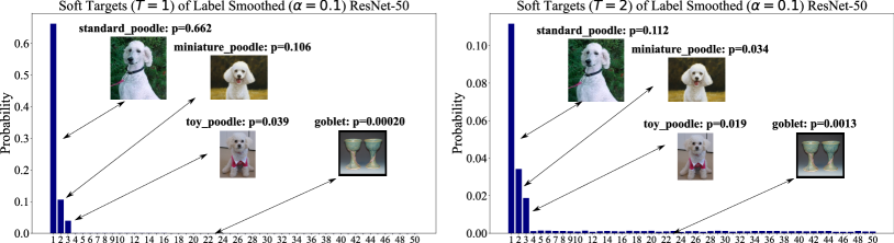
Figure 2: Soft output of the LS-trained ResNet-50 teacher $(\alpha=0.1)$ same as the one in Figure 1. Left: soft output at $T=1$; Right: soft output at $T=2$. The figures show the average of the soft outputs for 1300 training standard_poodle samples. Index 1 is the soft output for the standard_poodle class, i.e. ${p}^{t}_{k^{*}}(T)$. Index 2 and 3 are the soft outputs for the semantically similar classes miniature_poodle and toy_poodle respectively, i.e. ${p}^{t}_{ml}(T)$. The rest are soft outputs of randomly-chosen semantically dissimilar classes, i.e. ${p}^{t}_{ms}(T)$. Note that an increase of $T$ brings ${p}^{t}_{ml}(T)$ closer to ${p}^{t}_{k^{*}}(T)$. Therefore, soft targets at an increased $T$ encourage student to learn penultimate representations closer to semantically similar class $ml$, which are miniature_poodle and toy_poodle in this case. Therefore, in Figure 1 Observation 3, standard_poodle activations has more overlapping with miniature_poodle when KD of $T=2$ is used. Also, ${p}^{t}_{ms}(T)$ remains negligible after $T$ scaling, as shown in the figure. Furthermore, the figure of $T=1$ (Left) suggests that even with LS probabilities of incorrect classes $\{{p}^{t}_{m}\}$ are not all the same, and information erasure is not prefect in practice. Therefore, the diffusion of penultimate representations is not isotopic.

Why is this diffusion systematic and not isotopic? We revisit discussion from Hinton et al. (2015) to motivate the intuition behind this systematic diffusion. Hinton et al. (2015) introduce $T$ to scale the logits at the final softmax in order to produce soft targets that are more suitable for transfer. As argued by Hinton et al. (2015) on MNIST classification, a sample of ‘2’ may be assigned a probability of $10^{-6}$ of being a ‘3’ and $10^{-9}$ of being a 7. The resemblance between ‘2’ and ‘3’ is valuable information, but a probability of $10^{-6}$ has negligible influence on the loss when distilling to student. Hinton et al. (2015) introduce a temperature $T$ to emphasize the probabilities of such incorrect classes: during KD, their $T$-scaled counterparts have more noticeable effects on the student. On the other hand, the effect of $T$ scaling on the probability of $10^{-9}$ is negligible; consequently, the $T$-scaled counterparts of such probabilities remain to have unnoticeable effects on the student.

In particular, for a given sample of ground-truth class $k^{*}$, we let ${p}^{t}_{k^{*}}$ represent the probability of the correct class output by the teacher, ${p}^{t}_{m}$ represent the probability of one of the $K-1$ incorrect classes. Among these $K-1$ ${p}^{t}_{m}$, one or a few could be significantly larger than the other; we refer such probability as ${p}^{t}_{ml}$ (i.e.: probability of being a 3 in the above example). In particular, the class $ml$ is usually a semantically similar class of class $k^{*}$, therefore ${p}^{t}_{ml}$ is not negligible for a class $k^{*}$ sample (See Figure 2). For the rest of ${p}^{t}_{m}$ which are almost zero (noise level), we refer them as ${p}^{t}_{ms}$ (e.g., probability of being a 7 in the above example). Therefore, $\{{p}^{t}_{m}\}=\{{p}^{t}_{ml}\}\cup\{{p}^{t}_{ms}\}$. Usually, we have ${p}^{t}_{ml}\gg{p}^{t}_{ms}$ and ${p}^{t}_{ms}\approx 0$. We remark that $\{{p}^{t}_{m}\}$ are not all the same and can be observed even for an LS-trained teacher. It is because logits’ information is not completely erased (see Figure 2).

When KD of an increased $T$ is used, the soft output of the teacher is scaled and becomes $\mathbf{p}^{t}(T)$. In particular, the effect of $T$ scaling is to bring ${p}^{t}_{ml}$ closer to ${p}^{t}_{k^{*}}$, i.e., ${p}^{t}_{ml}(T)$ is closer to ${p}^{t}_{k^{*}}(T)$ relatively. Consequently, with soft target $\mathbf{p}^{t}(T)$, student is encouraged to produce a penultimate representation of a class $k^{*}$ sample that is closer to the incorrect class $ml$. This results in systematic diffusion of representations of class $k^{*}$ towards the incorrect class $ml$. This can be observed in Figure 1 Observation 3 for standard_poodle activations (here class $ml$ being miniature_poodle), and similarly for miniature_poodle activations. On the other hand, because ${p}^{t}_{ms}$ is negligibly small, even with $T$ scaling ${p}^{t}_{ms}(T)$ remains negligible and has unnoticeable effect for student’s penultimate representation. Therefore, the diffusion due to an increased $T$ is not isotopic but towards semantically similar classes (class $ml$). We provide more detailed discussion on systematic diffusion in Supplementary E.

We remark that this systematic diffusion can sometimes be observed when using a teacher without LS, see Figure 1, row 2 subplot 1 and row 3 subplot 1. For a teacher without LS (i.e. no information erasure), this systematic diffusion could in fact be advantageous in some cases, as it improves generalization of the student network using the rich logits’ information about instance resemblances. However, we focus on our thesis statement: compatibility between LS and KD. In our case, systematic diffusion in student due to KD at an increased $T$ curtails the distance enlargement (between semantically similar classes) benefits of using an LS-trained teacher, rendering KD ineffective.

5 Empirical Studies

In this section, we conduct large-scale image classification (standard, fine-grained) LS-KD experiments. We remark that LS and KD are compatible when with all the other factors fixed (including $T$), student distilled from an LS-trained teacher outperforms the student distilled from a teacher trained without LS. We use ResNet-50 teacher and ResNet-18, ResNet-50 students using ImageNet-1K and CUB200-2011 datasets following similar procedure as Shen et al. (2021b). Results are shown in Table 2.

Table 2: KD results from ResNet-50 Teacher to ResNet-18, ResNet-50 students for (A) standard image classification using ImageNet-1K and (B) fine-grained image classification using CUB200-2011 benchmarks following similar procedure as Shen et al. (2021b). We show the top1/ top5 test accuracies. Configurations where LS and KD are compatible are in bold. As one can clearly observe, with LS-trained teacher, there is a consistent degrade in student performance as $T$ increases. This can be observed in all our 34 experiments. These results comprehensively support our claim: in the presence of an LS-trained teacher, KD at higher temperatures is rendered ineffective. On the other hand, we observe that higher $T$ can improve the performance of ResNet-18 student when using a teacher trained without LS in fine-grained classification using CUB200-2011 (B). i.e.: We observe improvement of ResNet-18 student from $T=1$ to $T=2$, $T=3$ when distilling from teacher trained without LS in (B). We particularly emphasize that our findings are exclusive to LS and KD: That is in the presence of an LS-trained teacher, higher $T$ renders ineffective KD due to systematic diffusion. All these results are averaged over 3 independent runs. Standard deviations are reported in Supplementary Tables D.1, D.2 respectively.

A. ImageNet-1K : ResNet-50 to ResNet-18, ResNet-50 KD $\alpha$ = 0.0 $\alpha$ = 0.1 Teacher : ResNet-50 - 76.130 / 92.862 76.196 / 93.078 Student : ResNet-18 $T$ = 1 71.547 / 90.297 71.616 / 90.233 $T$ = 2 71.349 / 90.359 68.428 / 89.139 $T$ = 3 69.570 / 89.657 66.570 / 88.631 $T$ = 64 66.230 / 88.730 65.472 / 89.564 Student : ResNet-50 $T$ = 1 76.502 / 93.059 77.035 / 93.327 $T$ = 2 76.198 / 92.987 76.101 / 93.115 $T$ = 3 75.388 / 92.676 75.821 / 93.065 $T$ = 64 74.291 / 92.399 74.627 / 92.639

B. CUB200-2011 : ResNet-50 to ResNet-18, ResNet-50 KD $\alpha$ = 0.0 $\alpha$ = 0.1 Teacher : ResNet-50 - 81.584 / 95.927 82.068 / 96.168 Student : ResNet-18 $T$ = 1 80.169 / 95.392 80.946 / 95.312 $T$ = 2 80.808 / 95.593 80.428 / 95.518 $T$ = 3 80.785 / 95.674 78.196 / 95.213 $T$ = 64 73.611 / 94.529 67.161 / 93.062 Student : ResNet-50 $T$ = 1 82.902 / 96.358 83.742 / 96.778 $T$ = 2 82.534 / 96.427 83.379 / 96.537 $T$ = 3 82.091 / 96.243 82.142 / 96.427 $T$ = 64 79.784 / 95.927 77.206 / 95.812

Penultimate layer visualization analysis. We show this systematic diffusion in ResNet-18 student using Figure 1 Observation 3. We focus on the two semantically similar classes: miniature_poodle, standard_poodle. Given the same LS-trained ResNet-50 teacher and using the exact distillation process, we observe that at increased temperatures ($T=1$ to $T=3$), the above semantically similar classes start to diffuse. We also observe that class submarine diffuses towards another class which is semantically similar to submarine (not shown in the figure). Because of this systematic diffusion, the central cluster distances between miniature_poodle and standard_poodle reduces with increased $T$ in the presence of LS-trained teacher. Consequently, this systematic diffusion results in detrimental performance in the student causing an accuracy drop of 5.05% as shown in Table 2 A. Supporting visualization showing systematic diffusion in ResNet-50 student shown in Figure A.4 corresponding to the 1.21% drop as shown in Table 2. CUB200-2011 visualization for ResNet-18 and ResNet-50 students shown in Figures A.3, A.4 respectively.

Analysis using diffusion index ($\eta$). We quantitatively illustrate systematic diffusion in the ResNet-18, ResNet-50 students using $\eta$ for 10 target classes in Table 3. We clearly observe that $\eta(T_{1}=1,T_{2}=3;\pi,S_{1})<0$ and $\eta(T_{1}=1,T_{2}=3;\pi,S_{2})>0$ for all these 10 target classes, thereby quantitatively showing that the penultimate layer representations are diffused towards semantically similar classes when distilled from an LS-trained teacher at a larger temperature. This systematic diffusion results in detrimental performance of the student resulting in an accuracy drop of 5.05%, 1.21% for ResNet-18 and ResNet-50 students respectively as shown in Table 2 A. We also include a rich study on selecting $S_{1}$ and $S_{2}$ in Supplementary G.

Table 3: $\eta$ analysis for ResNet-18 (top), ResNet-50 (bottom) students for 10 target classes in ImageNet-1K (We show in 2 sets). We use standard, pre-defined ImageNet-1K knowledge graph derived from WordNet (Fellbaum, 1998) as a prior to select 4 semantically similar classes and 20 semantically dissimilar classes (random) to compute the diffusion index $\eta$. $|S_{1}|=4$ and $|S_{2}|=20$ for each target class. We demonstrate that when increasing $T=1$ to $T=3$, the diffusion index $\eta$ between target class and $S_{1}$ reduces substantially and vice versa for $S_{2}$ shown for both training and validation set. This quantitatively shows systematic diffusion when distilling at higher $T$ in the presence of an LS-trained teacher.

Set 1 : ResNet-18 student Target class $Train:S_{1}$ $Train:S_{2}$ $Val:S_{1}$ $Val:S_{2}$ Chesapeake Bay retriever -0.392 0.162 -1.082 0.269 curly-coated retriever -0.578 0.179 -2.024 0.383 flat-coated retriever -1.729 0.380 -3.320 0.655 golden retriever -0.880 0.228 -2.594 0.555 Labrador retriever -2.758 0.501 -4.618 0.840	Set 2 : ResNet-18 student Target class $Train:S_{1}$ $Train:S_{2}$ $Val:S_{1}$ $Val:S_{2}$ thunder snake -2.316 0.376 -3.584 0.511 ringneck snake -0.463 0.058 -0.757 0.094 hognose snake -1.528 0.258 -4.067 0.631 water snake -2.028 0.326 -3.053 0.478 king snake -2.474 0.521 -4.577 0.840
Set 1 : ResNet-50 student Target class $Train:S_{1}$ $Train:S_{2}$ $Val:S_{1}$ $Val:S_{2}$ Chesapeake_Bay_retriever -1.061 0.180 -1.346 0.240 curly-coated_retriever -0.764 0.127 -1.193 0.207 flat-coated_retriever -0.983 0.169 -0.331 0.056 golden_retriever -0.744 0.159 -0.911 0.182 Labrado_retriever -1.336 0.236 -1.468 0.257	Set 2 : ResNet-50 student Target class $Train:S_{1}$ $Train:S_{2}$ $Val:S_{1}$ $Val:S_{2}$ thunder snake -2.565 0.417 -0.778 0.105 ringneck snake -2.224 0.358 -0.726 0.102 hognose snake -3.748 0.623 -2.173 0.342 water snake -1.631 0.258 -0.390 0.037 king snake -1.969 0.339 0.956 -0.159

Resolving the contradictory claims using systematic diffusion. The seemingly contradictory findings of Müller et al. (2019) and Shen et al. (2021b) can be resolved using our discovery on systematic diffusion as follows: Müller et al. (2019) make the incompatibility claim between LS and KD due to observing students distilled from LS-trained teacher performing inferior to students distilled from teacher trained without LS at higher $T$. On the contrary, Shen et al. (2021b) make the compatibility claim between LS and KD due to observing students distilled from LS-trained teacher performing superior to students distilled from teacher trained without LS at lower $T$ (i.e.: $T=1$). Critically, our main finding shows that in the presence of an LS-trained teacher, KD at higher temperatures systematically diffuses penultimate layer representations learnt by the student towards semantically similar classes. This systematic diffusion essentially curtails the distance enlargement (between semantically similar classes) benefits of distilling from an LS-trained teacher, thereby rendering KD at increased temperatures ineffective. More specifically, in the presence of an LS-trained teacher, the degree of systematic diffusion is low when distilling at lower $T$ thereby making LS and KD compatible. On the other hand, the degree of systematic diffusion is relatively higher when distilling at higher $T$, thereby making LS and KD incompatible. Our findings are summarized in Table 1. Importantly, systematic diffusion was the missing concept that is instrumental in resolving the contradictory claims of Müller et al. (2019) and Shen et al. (2021b).

6 Extended Experiments

Compact Student Distillation. KD is one of the most prominent methods used for neural network compression. Hence, we conduct KD experiments to transfer knowledge to compact student model. We conduct fine-grained classification experiments (CUB200-2011) using ResNet-50 teacher (25.6M params) and MobileNet-V2 student (3.50M params). The results are shown in Table 4. Our results show that in the presence of an LS-trained teacher, KD at higher temperatures is rendered ineffective due to systematic diffusion in the student. We also show supporting results for EfficientNet-B0 (for ImageNet-1K classification): Table B.3. Visualization : Figure A.2 and $\eta$ results : Table B.4.

Table 4: Compact student distillation results: Top1/ Top5 Accuracy for KD experiments from ResNet-50 Teacher to MobileNetV2 student using CUB200-2011. Configurations where LS and KD are compatible are in bold. These results support our claim: in the presence of an LS-trained teacher, KD at higher temperatures is rendered ineffective. We also observe that higher $T$ is helpful when distilling from a teacher trained without LS in this setup (Observe improvement of student from $T=1$ to $T=2$, $T=3$ when distilling from teacher trained without LS). Standard deviations reported in Table D.4.

$\alpha$ = 0.0 $\alpha$ = 0.1 Teacher : ResNet-50 - 81.584 / 95.927 82.068 / 96.168 Student : MobileNet-V2 $T$ = 1 81.144 / 95.677 81.731 / 95.754 $T$ = 2 81.895 / 95.858 80.609 / 95.47 $T$ = 3 81.257 / 95.677 78.961 / 95.306 $T$ = 64 75.441 / 94.702 70.435 / 93.494

Neural machine translation. Following Shen et al. (2021b), we conduct KD experiments for neural machine translation task using IWSLT dataset. We report English $\rightarrow$ German translation results in Table 5. Our results comprehensively show that in the presence of an LS-trained teacher, KD at higher temperatures is rendered ineffective due to systematic diffusion in the student. We also show supporting results for English $\rightarrow$ Russian translation in Table B.2.

Table 5: Neural Machine Translation results: BLEU scores for KD experiments for Transformer Teacher to Transformer student on IWSLT dataset using English $\rightarrow$ German translation task. Configurations where LS and KD are compatible are in bold. These results comprehensively support our claim: in the presence of an LS-trained teacher, KD at higher temperatures is rendered ineffective. Standard deviations reported in Table D.3.

$\alpha$ = 0.0 $\alpha$ = 0.1 Teacher : Transformer - 26.461 26.750 Student : Transformer $T$ = 1 24.914 25.085 $T$ = 2 23.103 23.421 $T$ = 3 21.999 22.076 $T$ = 64 6.564 6.461

7 Discussion and Conclusion

Discussion. While increased $T$ is believed to be a helpful empirical trick (Also observed in many of our experiments when distilling from a teacher trained without LS) to produce better soft-targets for KD, we convincingly show that in the presence of LS-trained teacher, an increased $T$ causes systematic diffusion in the student. This systematic diffusion directly curtails the distance enlargement (between semantically similar classes) benefits of an LS-trained teacher, thereby rendering KD ineffective at increased $T$. For practitioners, as a rule of thumb, we suggest to use an LS-trained teacher with a low-temperature transfer (i.e. $T=1$) to render high performance students. We also remark that our finding on systematic diffusion substantially reduces the search space for the intractable parameter $T$ when using an LS-trained teacher. Our findings are summarized in Table 1. With increasing use of KD, we hope that our findings can benefit various applications including neural architecture search (Li et al., 2020a; Yu et al., 2020; Wang et al., 2021), self-supervised learning (Fang et al., 2021; Abbasi Koohpayegani et al., 2020), compact deepfake / anomaly detection (Dzanic et al., 2020; Chandrasegaran et al., 2021; Lim et al., 2018; Tran et al., 2021) and GAN compression (Li et al., 2020b; Fu et al., 2020; Yu & Pool, 2020).

Conclusion. Focusing on the compatibility between LS and KD, we have conducted an empirical study to investigate the seemingly contradictory findings of Müller et al. (2019) and Shen et al. (2021b). Through comprehensive scrutiny of these works, we discover an intriguing phenomenon called systematic diffusion: That is in the presence of an LS-trained teacher, KD at higher temperatures systematically diffuses penultimate layer representations learnt by the student towards semantically similar classes. This systematic diffusion essentially curtails the benefits of distilling from an LS-trained teacher, thereby rendering KD at increased temperatures ineffective. We showed this systematic diffusion both qualitatively and quantitatively using extensive analysis. We also supported our findings with large scale experiments including image classification (standard, fine-grained), neural machine translation and compact student distillation tasks. Critically, our discovery on systematic diffusion was the missing concept that is instrumental in resolving the contradictory findings of Müller et al. (2019) and Shen et al. (2021b), thereby establishing a foundational understanding on the compatibility between LS and KD.

Acknowledgements. This research is supported by the National Research Foundation, Singapore under its AI Singapore Programmes (AISG Award No.: AISG2-RP-2021-021; AISG Award No.: AISG-100E2018-005). This project is also supported by SUTD project PIE-SGP-AI-2018-01. We also gratefully acknowledge the support of NVIDIA AI Technology Center (NVAITC) for our research.

Supplementary Materials

Contents of this Supplementary

This Supplementary provides additional experiments, results (penultimate layer visualization and $\eta$ analysis), case studies and analyses to further support our main finding on Systematic diffusion. The Supplementary materials are organized as follows:

• Section A: Additional Penultimate Layer Visualizations

• Section B: Additional Experiments / Analysis

• Section C : Research Reproducibility Details

• Section D: Standard Deviation for main paper experiments

• Section E: Additional Discussion: Why this diffusion is systematic and not isotopic?

• Section F: Algorithm for Projection and visualization of penultimate layer representations

• Section G: Semantically similar / dissimilar classes

  • Section G.1: Using standard, pre-defined ImageNet knowledge graph as a prior

  • Section G.2: Using distance in the feature space

• Section H: Case study: Smoothness of targets are insufficient to determine KD performance

  • Section H.1: Case study at lower $T$ with same degree of smoothness

  • Section H.2: Case study at moderately higher $T$ with same degree of smoothness

  • Section H.3: Case study at very high $T$ with same degree of smoothness

• Section I: Class-wise accuracy for target classes

• Section J: Additional Exploration of $\alpha$ and $T$

• Section K: Alternative characterization of cluster distance

• Section L: Sample images of different classes used in the study

Appendix A Additional Penultimate Layer Visualizations

In this section, we show additional penultimate layer visualizations to support our finding on systematic diffusion. The details are included in Table A.1.

Table A.1: Penultimate layer visualization details supporting our finding on systematic diffusion. Our visualizations cover multiple tasks including image classification (standard, fine-grained) and compact student distillation tasks spanning across multiple datasets and teacher-student architectures.

Teacher / Student Dataset Visualization ResNet-50 / ResNet-18 ImageNet-1K Figure 1 ResNet-50 / ResNet-50 ImageNet-1K Figure A.1 ResNet-50 / EfficientNet-B0 ImageNet-1K Figure A.2 ResNet-50 / ResNet-18 CUB200 Figure A.3 ResNet-50 / ResNet-50 CUB200 Figure A.4 ResNet-50 / ConvNext-T CUB200 Figure A.5

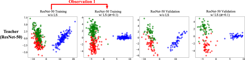
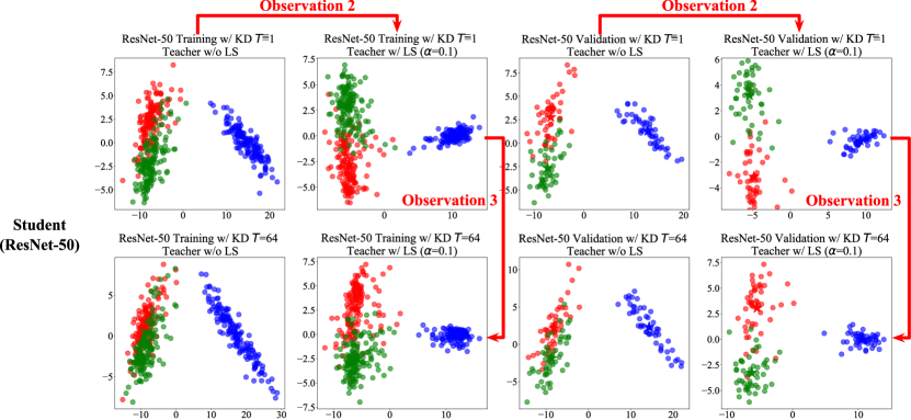
Figure A.1: Visualization of the penultimate layer representations (Teacher = ResNet-50, Student = ResNet-50, Dataset = ImageNet). We follow the same setup and procedure used in Müller et al. (2019) and Shen et al. (2021b). We also follow their three-class analysis: two semantically similar classes ( miniature_poodle, standard_poodle) and one semantically different class ( submarine). Observation 1: The use of LS on the teacher leads to tighter clusters and erasure of logits’ information as claimed by Müller et al. (2019). In addition, increase in central distance between semantically similar classes ( miniature_poodle, standard_poodle) as claimed by Shen et al. (2021b) can be observed. Observation 2: We further visualize the student’s representations. Increase in central distance between semantically similar classes can also be observed. This confirms the transfer of this benefit from the teacher to the student. Note that in Müller et al. (2019) and Shen et al. (2021b), student’s representations have not been visualized. Observation 3 (Our main discovery): KD of an increased $T$ causes systematic diffusion of representations between semantically similar classes ( miniature_poodle, standard_poodle). Since the student is also a very powerful network (ResNet-50), the extent of this systematic diffusion is not large compared to the ResNet-18 student. We further show $\eta$ analysis in Table 3 to quantitatively show this systematic diffusion. We also show image samples for these 3 classes in Figure L.1. Best viewed in color.

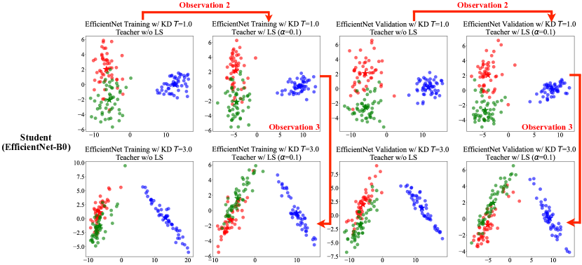
Figure A.2: Visualization of the penultimate layer representations (Teacher = ResNet-50, Student = EfficientNet-B0, Dataset = ImageNet). We follow the same setup and procedure used in Müller et al. (2019) and Shen et al. (2021b). We also follow their three-class analysis: two semantically similar classes ( miniature_poodle, standard_poodle) and one semantically different class ( submarine). Observation 1: The use of LS on the teacher leads to tighter clusters and erasure of logits’ information as claimed by Müller et al. (2019). In addition, increase in central distance between semantically similar classes ( miniature_poodle, standard_poodle) as claimed by Shen et al. (2021b) can be observed. Observation 2: We further visualize the student’s representations. Increase in central distance between semantically similar classes can also be observed. This confirms the transfer of this benefit from the teacher to the student. Note that in Müller et al. (2019) and Shen et al. (2021b), student’s representations have not been visualized. Observation 3 (Our main discovery): KD of an increased $T$ causes systematic diffusion of representations between semantically similar classes ( miniature_poodle, standard_poodle). We also show image samples for these 3 classes in Figure L.1. Best viewed in color.

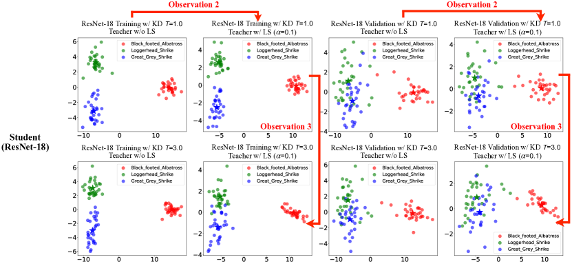
Figure A.3: Visualization of the penultimate layer representations (Teacher = ResNet-50, Student = ResNet-18, Dataset = CUB200-2011). We follow the same setup and procedure used in Müller et al. (2019) and Shen et al. (2021b). We also follow their three-class analysis: two semantically similar classes ( Loggerhead_Shrike, Great_Grey_Shrike) and one semantically different class ( Black_footed_Albatross). Observation 1: The use of LS on the teacher leads to tighter clusters and erasure of logits’ information as claimed by Müller et al. (2019). In addition, increase in central distance between semantically similar classes ( Loggerhead_Shrike, Great_Grey_Shrike) as claimed by Shen et al. (2021b) can be observed. Observation 2: We further visualize the student’s representations. Increase in central distance between semantically similar classes can also be observed. This confirms the transfer of this benefit from the teacher to the student. Note that in Müller et al. (2019) and Shen et al. (2021b), student’s representations have not been visualized. Observation 3 (Our main discovery): KD of an increased $T$ causes systematic diffusion of representations between semantically similar classes ( Loggerhead_Shrike, Great_Grey_Shrike). We also show image samples for these 3 classes in Figure L.2. Best viewed in color.

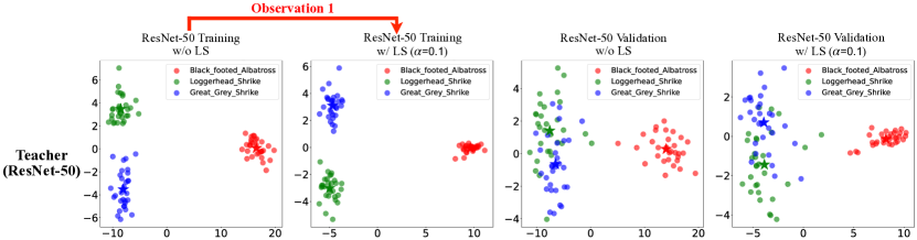
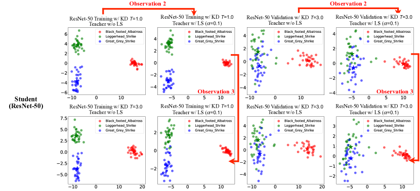
Figure A.4: Visualization of the penultimate layer representations (Teacher = ResNet-50, Student = ResNet-50, Dataset = CUB200-2011). We follow the same setup and procedure used in Müller et al. (2019) and Shen et al. (2021b). We also follow their three-class analysis: two semantically similar classes ( Loggerhead_Shrike, Great_Grey_Shrike) and one semantically different class ( Black_footed_Albatross). Observation 1: The use of LS on the teacher leads to tighter clusters and erasure of logits’ information as claimed by Müller et al. (2019). In addition, increase in central distance between semantically similar classes ( Loggerhead_Shrike, Great_Grey_Shrike) as claimed by Shen et al. (2021b) can be observed. Observation 2: We further visualize the student’s representations. Increase in central distance between semantically similar classes can also be observed. This confirms the transfer of this benefit from the teacher to the student. Note that in Müller et al. (2019) and Shen et al. (2021b), student’s representations have not been visualized. Observation 3 (Our main discovery): KD of an increased $T$ causes systematic diffusion of representations between semantically similar classes ( Loggerhead_Shrike, Great_Grey_Shrike). We also show image samples for these 3 classes in Figure L.2. Best viewed in color.

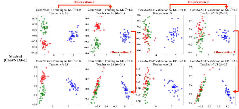
Figure A.5: Visualization of the penultimate layer representations (Teacher = ResNet-50, Student = ConvNeXt-T, Dataset = CUB200-2011). We follow the same setup and procedure used in Müller et al. (2019) and Shen et al. (2021b). We also follow their three-class analysis: two semantically similar classes ( Loggerhead_Shrike, Great_Grey_Shrike) and one semantically different class ( Black_footed_Albatross). Observation 1: The use of LS on the teacher leads to tighter clusters and erasure of logits’ information as claimed by Müller et al. (2019). In addition, increase in central distance between semantically similar classes ( Loggerhead_Shrike, Great_Grey_Shrike) as claimed by Shen et al. (2021b) can be observed. Observation 2: We further visualize the student’s representations. Increase in central distance between semantically similar classes can also be observed. This confirms the transfer of this benefit from the teacher to the student. Note that in Müller et al. (2019) and Shen et al. (2021b), student’s representations have not been visualized. Observation 3 (Our main discovery): KD of an increased $T$ causes systematic diffusion of representations between semantically similar classes ( Loggerhead_Shrike, Great_Grey_Shrike). We also show image samples for these 3 classes in Figure L.2. Best viewed in color.

Appendix B Additional Experiments / Analysis

Fine-grained image classification. We conduct experiments using an additional student architecture, ConvNeXt-T (Liu et al., 2022) to further support our findings. The results are shown in Table B.1. We show systematic diffusion using penultimate layer visualizations in Figure A.5.

Table B.1: Top1 / Top5 accuracies for fine-grained classification (CUB200) using ConvNeXt-T student. We use $T=1,T=3$ for distilling knowledge from ResNet-50 teacher. As one can clearly observe, with LS-trained teacher, there is a consistent degrade in student performance as $T$ increases. This can be observed in all our 34 experiments. These results comprehensively support our claim: in the presence of an LS-trained teacher, KD at higher temperatures is rendered ineffective.

$\alpha=0.0$ $\alpha=0.1$ Teacher : ResNet-50 - 81.584 / 95.927 82.068 / 96.168 Student : $T$ = 1 86.624 / 97.221 86.866 / 97.377 ConvNeXt-T $T$ = 3 86.554 / 97.187 83.638 / 97.135

Neural Machine Translation. We conduct additional KD experiments for English $\rightarrow$ Russian translation using IWSLT dataset. We report BLUE scores in Table B.2. We remark that all these experiments comprehensively support our main finding on systematic diffusion.

Table B.2: BLEU scores for KD experiments from Transformer Teacher to Transformer student on IWSLT dataset using English $\rightarrow$ Russian translation task, following the similar procedure as Shen et al. (2021b). Configurations where LS and KD are compatible are in bold. As one can clearly observe, with LS-trained teacher, there is a consistent degrade in student performance as $T$ increases. This can be observed in all our 34 experiments. These results comprehensively support our claim: in the presence of an LS-trained teacher, KD at higher temperatures is rendered ineffective.

$\alpha$ = 0.0 $\alpha$ = 0.1 Teacher : Transformer - 16.718 16.976 Student : Transformer $T$ = 1 16.140 16.197 $T$ = 2 14.977 15.100 $T$ = 3 13.826 14.106 $T$ = 64 3.605 3.590

Compact Student Distillation. We conduct experiments using an additional compact student architecture, EfficientNet-B0 (Tan & Le, 2019) (5.3M params) to further support our findings. We use ResNet-50 as the teacher model and perform large-scale experiments using ImageNet-1K. The results are shown in Table B.3. We show systematic diffusion using penultimate layer visualizations in Figure A.2 and $\eta$ results are shown in Table B.4.

Table B.3: Top1 / Top5 accuracies for compact student distillation (ImageNet-1K) using EfficientNet-B0 student. We use $T=1,T=3$ for distilling knowledge from ResNet-50 teacher. As one can clearly observe, with LS-trained teacher, there is a consistent degrade in student performance as $T$ increases. This can be observed in all our 34 experiments. These results comprehensively support our claim: in the presence of an LS-trained teacher, KD at higher temperatures is rendered ineffective.

$\alpha=0.0$ $\alpha=0.1$ Teacher : ResNet-50 - 76.130 / 92.862 76.196 / 93.078 Student : $T$ = 1 68.850 / 88.604 69.906 / 89.284 EfficientNet-B0 $T$ = 3 68.546 / 88.704 58.182 / 83.918

Table B.4: $\eta$ calculation for EfficientNet-B0 for 10 target classes (exact classes used in Table 3 main paper). Our finding is consistently observed (see main paper). We clearly show that $\eta(T_{1}=1,T_{2}=3;\pi,S_{1})<0$ and $\eta(T_{1}=1,T_{2}=3;\pi,S_{2})>0$ for all these 10 target classes, thereby quantitatively demonstrating our discovery on systematic diffusion.

Set 1 Target class $Train:S_{1}$ $Train:S_{2}$ $Val:S_{1}$ $Val:S_{2}$ Chesapeake_Bay_retriever -2.276 0.490 -3.760 0.790 curly-coated_retriever -0.830 0.235 -4.502 0.933 flat-coated_retriever -0.979 0.173 -3.904 0.807 golden_retriever -3.651 0.694 -4.356 0.890 Labrado_retriever -2.747 0.469 -4.730 0.860

Set 2 Target class $Train:S_{1}$ $Train:S_{2}$ $Val:S_{1}$ $Val:S_{2}$ thunder_snake -10.981 1.458 -12.916 1.789 ringneck_snake -9.629 1.211 -10.617 1.373 hognose_snake -7.984 1.271 -9.347 1.536 water_snake -8.217 1.302 -9.645 1.489 king_snake -8.371 1.365 -10.082 1.647

Advanced KD methods. We demonstrate our finding using a popular advanced KD method by Heo et al. (2019). This method performs optimized feature distillation (contains margin-ReLU feature transforms, partial L2 distance functions, optimized feature positions) combined with task loss (In our experiments, the task is KD) . The results are shown in Table B.5. We show that advanced KD methods also suffer from systematic diffusion when distilling from an LS-trained teacher at larger $T$.

Table B.5: Advanced KD results using method proposed by (Heo et al., 2019): We show top1 / top5 accuracies for fine-grained classification (CUB200) using ResNet-50 teacher to ResNet-50 student. We use $T=1,T=3$ for distilling knowledge from ResNet-50 teacher. As one can clearly observe, with LS-trained teacher, there is a consistent degrade in student performance as $T$ increases when using advanced KD methods. These results comprehensively support our claim: in the presence of an LS-trained teacher, KD at higher temperatures is rendered ineffective.

$\alpha=0.0$ $\alpha=0.1$ Teacher : ResNet-50 - 81.584 / 95.927 82.068 / 96.168 Student : ResNet-50 $T$ = 1 82.568 / 96.479 83.794 / 96.686 Advanced KD $T$ = 3 82.706 / 96.307 81.739 / 96.117

Appendix C Research Reproducibility Details

Code / Pre-trained models. Pytorch code to reproduce all our results and analysis can be found at https://keshik6.github.io/revisiting-ls-kd-compatibility/. All pretrained models for image classification using ImageNet-1K, fine-grained classification using CUB200-2011, neural machine translation using IWSLT and compact student distillation are available at https://keshik6.github.io/revisiting-ls-kd-compatibility/.

Docker information : To allow for training in containerised environments (HPC, Super-computing clusters), please use nvcr.io/nvidia/pytorch:20.12-py3 container.

Experiment details and hyper-parameters:

ImageNet-1K: For ImageNet experiments, we follow similar setup as Shen et al. (2021b) and use ILSVRC2012 version. For training LS networks, we train for 90 epochs with initial learning rate 0.1 decayed by a factor of 10 every 30 epochs. For KD experiments, we train for 200 epochs with initial learning rate 0.1 decayed by a factor of 10 every 80 epochs. We conducted a grid search for hyper-parameters as well. For all experiments, we use a batch size of 256 and SGD with momentum 0.9 . For data augmentation, we use random crops and random horizontal flips. All experiments were repeated 3 times. For visualization of penultimate layer representations, we use 150 samples for training set and 50 samples for validation set.

Fine-grained classification and compact student distillation. We follow similar setup as Shen et al. (2021b). For training both LS and KD networks, we train for 200 epochs with initial learning rate 0.01 decayed by a factor of 10 every 80 epochs. We conducted a grid search for hyper-parameters as well. For all experiments, we use a batch size of 256 and SGD with momentum 0.9 . All experiments were repeated 3 times. For data augmentation, we use random crops, random rotation, color jitter and random horizontal flips. For visualization of penultimate layer representations, we use all samples for training and validation sets.

Neural Machine Translation We use IWSLT dataset. We follow similar setup as Shen et al. (2021b). We use Adam as the optimizer, lr with 0.0005, dropout with drop rate as 0.3, weight-decay with 0 and max tokens with 4096, all of these hyper-parameters are following settings of Shen et al. (2021b). These hyper-parameters were used for both translation tasks (English $\rightarrow$ German, English $\rightarrow$ Russian). We use the code here similar to Shen et al. (2021b).

Appendix D Standard Deviation for main paper experiments

In this section, we report the standard deviation for all KD experiments in the main paper. The standard deviation for ImageNet-1K and CUB200-2011 main paper experiments are reported in Tables D.1 and D.2 respectively. The standard deviation for Compact student distillation and neural machine translation main paper experiments are reported in Tables D.4 and D.3 respectively. All standard deviations are within acceptable range.

Table D.1: KD results from ResNet-50 Teacher to ResNet-18, ResNet-50 students with standard deviations, following similar procedure as Shen et al. (2021b) on ImageNet-1K (Deng et al., 2009). We show the top1/ top5 test accuracies. Configurations where LS and KD are compatible are in bold. As one can clearly observe, with LS-trained teacher, there is a consistent degrade in student performance as $T$ increases. This can be observed in all our 34 experiments. These results comprehensively support our claim: in the presence of an LS-trained teacher, KD at higher temperatures is rendered ineffective. On the other hand, we observe that higher $T$ can improve the performance when using a teacher trained without LS in fine-grained classification and compact student distillation experiments (See Table 2 (B) and Table 4) All these results are averaged over 3 independent runs. The standard deviations are well within acceptable range.

$\alpha$ = 0.0 $\alpha$ = 0.1 Student : ResNet-18 $T$ = 1 71.547 $\pm$ 0.122 / 90.297 $\pm$ 0.175 71.616 $\pm$ 0.114 / 90.233 $\pm$ 0.119 $T$ = 2 71.349 $\pm$ 0.017 / 90.359 $\pm$ 0.054 68.799 $\pm$ 0.065 / 89.279 $\pm$ 0.092 $T$ = 3 69.570 $\pm$ 0.320 / 89.657 $\pm$ 0.041 67.699 $\pm$ 0.079 / 89.043 $\pm$ 0.096 $T$ = 64 66.230 $\pm$ 0.036 / 88.730 $\pm$ 0.071 64.506 $\pm$ 0.142 / 87.811 $\pm$ 0.100 Student : ResNet-50 $T$ = 1 76.502 $\pm$ 0.234 / 93.059 $\pm$ 0.061 77.035 $\pm$ 0.061 / 93.327 $\pm$ 0.185 $T$ = 2 76.198 $\pm$ 0.035 / 92.987 $\pm$ 0.105 76.101 $\pm$ 0.105 / 93.115 $\pm$ 0.017 $T$ = 3 75.388 $\pm$ 0.095 / 92.676 $\pm$ 0.006 75.821 $\pm$ 0.006 / 93.065 $\pm$ 0.088 $T$ = 64 74.291 $\pm$ 0.014 / 92.399 $\pm$ 0.035 74.627 $\pm$ 0.035 / 92.639 $\pm$ 0.085

Table D.2: KD results from ResNet-50 Teacher to ResNet-18, ResNet-50 students with standard deviations, following similar procedure as Shen et al. (2021b) on CUB200-2011 (Wah et al., 2011). We report top1/ top5 test accuracies. Configurations where LS and KD are compatible are in bold. As one can clearly observe, with LS-trained teacher, there is a consistent degrade in student performance as $T$ increases. This can be observed in all our 34 experiments. These results comprehensively support our claim: in the presence of an LS-trained teacher, KD at higher temperatures is rendered ineffective. On the other hand, we observe that higher $T$ can improve the performance when using a teacher trained without LS in fine-grained classification and compact student distillation experiments (See Table 2 and Table 4). These experiments are repeated for 3 independent runs and as you can observe the standard deviations are within acceptable range.

$\alpha$ = 0 $\alpha$ = 0.1 Student : ResNet-18 $T$ = 1 80.169 $\pm$ 0.336 / 95.392 $\pm$ 0.03 80.946 $\pm$ 0.03 / 95.312 $\pm$ 0.18 $T$ = 2 80.808 $\pm$ 0.314 / 95.593 $\pm$ 0.053 80.428 $\pm$ 0.053 / 95.518 $\pm$ 0.108 $T$ = 3 80.785 $\pm$ 0.26 / 95.674 $\pm$ 0.163 78.196 $\pm$ 0.163 / 95.213 $\pm$ 0.125 $T$ = 64 73.611 $\pm$ 0.314 / 94.529 $\pm$ 0.086 67.161 $\pm$ 0.086 / 93.062 $\pm$ 0.127 Student : ResNet-50 $T$ = 1 82.902 $\pm$ 0.343 / 96.358 $\pm$ 0.141 83.742 $\pm$ 0.141 / 96.778 $\pm$ 0.12 $T$ = 2 82.534 $\pm$ 0.137 / 96.427 $\pm$ 0.105 83.379 $\pm$ 0.105 / 96.537 $\pm$ 0.018 $T$ = 3 82.091 $\pm$ 0.161 / 96.243 $\pm$ 0.13 82.142 $\pm$ 0.13 / 96.427 $\pm$ 0.211 $T$ = 64 79.784 $\pm$ 0.26 / 95.927 $\pm$ 0.13 77.206 $\pm$ 0.13 / 95.812 $\pm$ 0.259

Table D.3: BLEU scores for KD experiments with standard deviations for Transformer Teacher to Transformer student on IWSLT dataset using English $\rightarrow$ German translation task, following the similar procedure as Shen et al. (2021b). Configurations where LS and KD are compatible are in bold. These results comprehensively support our claim: in the presence of an LS-trained teacher, KD at higher temperatures is rendered ineffective. These experiments are repeated for 3 independent runs and standard deviations are within acceptable range.

$\alpha$ = 0.0 $\alpha$ = 0.1 Student : Transformer $T$ = 1 24.914 $\pm$ 0.013 25.085 $\pm$ 0.082 $T$ = 2 23.103 $\pm$ 0.103 23.421 $\pm$ 0.039 $T$ = 3 21.999 $\pm$ 0.06 22.076 $\pm$ 0.125 $T$ = 64 6.564 $\pm$ 0.288 6.461 $\pm$ 0.061

Table D.4: KD results with standard deviations from ResNet-50 Teacher to MobileNet-V2 (Compact DNN) student using CUB200 Configurations where LS and KD are compatible are in bold. As one can clearly observe, with LS-trained teacher, there is a consistent degrade in student performance as $T$ increases. This can be observed in all our 34 experiments. These results comprehensively support our claim: in the presence of an LS-trained teacher, KD at higher temperatures is rendered ineffective. These experiments are repeated for 2 independent runs and as you can observe the standard deviations are within acceptable range.

$\alpha$ = 0.0 $\alpha$ = 0.1 Student : ResNet-18 $T$ = 1 81.144 $\pm$ 0.037 / 95.677 $\pm$ 0.062 81.731 $\pm$ 0.256 / 95.754 $\pm$ 0.098 $T$ = 2 81.895 $\pm$ 0.024 / 95.858 $\pm$ 0.000 80.609 $\pm$ 0.061 / 95.47 $\pm$ 0.159 $T$ = 3 81.257 $\pm$ 0.073 / 95.677 $\pm$ 0.012 78.961 $\pm$ 0.293 / 95.306 $\pm$ 0.196 $T$ = 64 75.441 $\pm$ 0.049 / 94.702 $\pm$ 0.025 70.435 $\pm$ 0.171 / 93.494 $\pm$ 0.025

Appendix E Additional Discussion: Why this diffusion is systematic and not isotopic?

We provide more perspective into why this diffusion is systematic and not isotopic. We use the LS-trained ResNet-50 teacher (same one in Figure 2) trained on ImageNet-1K to numerically show more evidence as to why this diffusion is systematic and not isotopic. Particularly we show that only very few classes (out of the 1000 classes in ImageNet-1K) have probabilities significantly larger than others. We examine the output probability for 3 classes: standard_poodle samples, golden_retriever samples and thunder_snake samples (We choose this classes randomly, similar analysis can be done for other classes as well).

For each class, we compute the average output probability for 1300 training samples, and observe following: Let $p_{1}$ be the largest probability which is also probability of the correct class.

• For the average probability of standard_poodle samples, the second largest probability, $p_{2}$ (miniature_poodle) is at least 100x larger than 976 other probabilities (out of 999 probabilities)

• For the average probability of golden_retriever samples, the second largest probability, $p_{2}$ (Labrador_retriever) is at least 100x larger than 924 other probabilities (out of 999 probabilities)

• For the average probability of thunder_snake samples, the second largest probability, $p_{2}$ (ringneck_snake) is at least 100x larger than 964 other probabilities (out of 999 probabilities)

Can this support the diffusion is systematic? We use results of standard_poodle for discussion. When KD of an increased T is used, these probabilities are scaled, and $p_{2}$ is brought closer to $p_{1}$, see Figure 2. Consequently, student is encouraged to produce penultimate layer representations of standard_poodle samples that are closer to miniature_poodle. This results in diffusion of penultimate layer representations of standard_poodle towards miniature_poodle, curtailing the distance enlargement benefit of distilling from an LS-trained teacher. For the 976 classes which have probabilities at least 100x smaller than that of miniature_poodle, even with T scaling, the probabilities remain negligible. They have no influence on the representation of standard_poodle. Therefore diffusion of standard_poodle will be towards miniature_poodle and several semantically similar classes but there is no diffusion towards these 976 classes. Therefore, the diffusion is systematic and is not isotopic.

In this discussion, we use 100x to mean significance/insignificance. If a probability $p_{i}$ is 100x smaller than another probability $p_{j}$, then even with $T$ scaling $p_{i}$ remains insignificant compared to $p_{j}$.

Appendix F Algorithm for Projection and visualization of penultimate layer representations

The algorithm for projection and visualization is included in 1 Müller et al. (2019). We also include a numpy style code of the projection / visualization algorithm in 2.

Algorithm 1 Projection and visualization of penultimate layer features

Input: \raisebox{-1pt}{1}⃝ High dimensional ($h$) features $(X,Y)$ of three classes extracted from penultimate layers of the trained model $f$ \raisebox{-1pt}{2}⃝ Model weight $w$ of the final layer of $f$

Output: The projected 2-D features $X^{\prime}$

  Compute the othonormal basis as $w^{\prime}$ = qr-decomposition ($w$) # dim = ($h$, 3)

  for all samples do

     Obtain the projected features on new basis via dot product: proj(X) = np.dot($X$, $w^{\prime}$) # dim = ($*$, 3)

     Dimension reduction from 3-D to 2-D via PCA(proj(X)) # dim = ($*$, 2)

  end forRETURN 2-D features: PCA(proj(X))

Algorithm 2 NumPy-style pseudo-code of the visualization algorithm

⬇

1# Inputs

2# weights_path: weights path of the final layer of your trained model

3# feature_path: feature path of the penultimate layer high dimension features extracted by your trained model

4

5# Outputs

6# 2-D features of each class

7

8# ------------------------------------------------------------------- #

9# Step 0. Init settings and select the class to visualize

10CLASSES = [’miniature_poodle’, ’standard_poodle’, ’submarine’]

11color = [’r’, ’g’, ’b’]

12model = ’resnet18’ # the student model

13

14# Step 1. Compute the orthonormal basis

15weights = np.load(weights_path) # load the final layer weights

16basis, _ = np.linalg.qr(weights.T) # dim=(*, 3)

17

18# Step 2. Load the extracted features

19num_sample = 150 # We sample 150 images per class

20output_feature = np.load(feature_path)

21

22# Step 3. Project the high dimension features to the new 3-D subspace

23output_project = np.dot(output_feature, basis)

24

25# Step 4. Dimension reduction from 3-D to 2-D using PCA

26pca = PCA(n_components=2)

27pca.fit(output_project)

28output_array = pca.transform(output_project)

29

30# Step 5. Plot the features on a 2-D plane

31for i, subclass in enumerate(CLASSES):

32 plt.scatter(output_array[i * num_sample:(i + 1) * num_sample, 0],

33 output_array[i * num_sample:(i + 1) * num_sample, 1],

34 c=color[i], label=subclass)

Appendix G Semantically similar / dissimilar classes

Given a target class $\pi$, let the set of semantically similar and dissimilar classes be $S_{1,},S_{2}$ respectively. In this section, we discuss two important methods for identifying $S_{1},S_{2}$ for the target class $\pi$.

G.1 Method 1: Using standard, pre-defined ImageNet knowledge graph as a prior

We use ImageNet hierarchy derived from WordNet (Fellbaum, 1998) to select semantically similar classes and semantically dissimilar classes to quantify systematic diffusion. WordNet (Fellbaum, 1998) is a laboriously hand-coded lexical database linking words into semantic relations including synonyms, hyponyms, and meronyms . Do note that ImageNet is organized using WordNet hierarchy. A web browser version of the ImageNet hierarchy can be accessed at this link (You can click any node to browse images that correspond to the associated synset)

We use this ImagNet hierarchy to select semantically similar classes and semantically dissimilar classes for the target class $\pi$. This way, we ensure the selection of semantically similar classes ($S_{1}$) and semantically dissimilar classes ($S_{2}$) is based on a strong prior (knowledge graph) to support our main finding.

G.2 Method 2: Using distance in the feature space to quantitatively define semantically similar / dissimilar classes

This method is a quantitative approach for defining semantically similar / dissimilar classes. Specifically, we consider the official ResNet-50 model trained on ImageNet-1K (classification). We use the validation set of ImageNet-1K and extract the penultimate layer representations for all the samples. For each class, we consider the centroid of the penultimate layer representations as the class prototype and calculate the centroid-centroid distance between all the classes (This will give a symmetric matrix of 1000 x 1000).

For selecting $S_{1}$: Next, for the target class $\pi$, we identify the closest 1% of classes (10 out of 999 classes) using the centroid-centroid distances. These would be the semantically similar classes to the target class as they have the smallest distances to the centroid of the target class.

For selecting $S_{2}$: Next, for the target class $\pi$, we identify the distant 90% of classes (900 out of 999 classes) using the centroid-centroid distances discussed above. These would be the semantically dissimilar classes to the target class as their centroids lie much far away from the centroid of the target class.

Consistency measurements between the 2 methods: Let the semantically similar and dissimilar classes identified using method 1 be $S_{1,qualitative},S_{2,qualitative}$ respectively. Let the semantically similar and dissimilar classes identified using method 1 be $S_{1,quantitative},S_{2,quantitative}$ respectively. In this section, we measure the consistency between qualitative selection of $S_{1,qualitative},S_{2,qualitative}$ (method 1) and the quantitative definition of $S_{1,quantitative},S_{2,quantitative}$ (method 2). This consistency measurements are shown for all the target classes in the Table G.1. As one can clearly observe both method 1 and method 2 agree 85% on average for semantically similar classes and 94% on average for semantically dissimilar classes. Do note that we use pre-defined knowledge graph for ImageNet-1K as prior (method 1) to select the semantically similar / dissimilar classes for our $\eta$ computation in Table 3.

Table G.1: Consistency measurements between using pre-defined knowledge graph for ImageNet-1K as prior vs. feature space distance method for identifying semantically similar / dissimilar classes. This table shows the agreement between these 2 methods in identifying semantically similar / dissimilar classes. Each row indicates the agreement between the 2 methods with respect to the target class. An agreement value of 1.000 indicates a perfect agreement between the 2 methods. As we can clearly observe on average both methods agree 85% for semantically similar classes and 94% for semantically dissimilar classes. This can suggest that we can leverage on either one of the methods to select the semantically similar / dissimilar classes for our analysis on systematic diffusion. Do note that we use pre-defined knowledge graph for ImageNet-1K as prior (method 1) to select the semantically similar / dissimilar classes for our $\eta$ computation in Table 3.

Target class $\frac{S_{1,qualitative}\cap S_{1,quantitative}}{\|S_{1,qualitative}\|}$ $\frac{S_{2,qualitative}\cap S_{2,quantitative}}{\|S_{2,qualitative}\|}$ Chesapeake Bay retriever 1.000 0.950 curly-coated retriever 0.750 0.950 flat-coated retriever 1.000 1.000 golden retriever 0.500 1.000 Labrador retriever 0.750 1.000 thunder_snake 1.000 0.900 ringneck_snake 1.000 0.900 hognose_snake 0.500 0.900 water_snake 1.000 0.900 king_snake 1.000 0.900 Average 0.850 0.940

Appendix H Case study: Smoothness of targets are insufficient to determine KD performance. Systematic diffusion is critical.

An interesting perspective is whether the degree of smoothness of targets produced by an LS-trained teacher can determine the KD performance (of the student). We acknowledge that smoothness of targets produced by the teacher at different temperatures is important. However, we quantitatively show that the degree of smoothness cannot adequately explain the KD performance in the presence of an LS-trained teacher. More specifically, we show that the KD performance in the presence of LS-trained teachers can be explained by our discovered systematic diffusion and not directly using the degree of smoothness. The detailed study is discussed below.

Our view: The degree of smoothness of targets is rather unable to explain the performance of KD. We show this using 3 comprehensive case studies comprising 7 counterexamples.

Measuring smoothness of targets: To perform a quantitative study to support our view, we measure the smoothness of the targets produced by the teacher. The target produced for every training sample by the teacher for KD is a discrete probability distribution. To measure the smoothness of this target, we can use entropy which is a very popular method. Entropy of a discrete probability distribution with $N$ classes can be indicated by $H(p)=\sum_{i}^{N}-p_{i}ln(p_{i})$ where $p_{i}$ indicates the probability assigned to the $i^{th}$ class. The maximum entropy/smoothness will be equal to $H_{max}(p)=ln(N)$ which corresponds to the uniform probability distribution over all classes. The key idea here is higher the entropy, smoother the target. We measure the average entropy for the training set (since this is the set used for distillation) to approximate the smoothness of the targets. Do note that the average entropy is measured using the targets produced by the teacher at different $T$.

Table H.1 shows the average entropy/ smoothness of the targets for the ResNet-50 teachers used in our CUB200-2011 experiments. Higher entropy indicates that the targets are over-smoothed. Do note that the maximum average entropy for CUB200-2011 (Wah et al., 2011) is $ln(200)\approx 5.298$.

H.1 Case study at lower $T$ with same degree of smoothness

Consider a lower $T$.

As shown in Table H.1, the entropy / smoothness of targets produced by LS-trained teacher ($\alpha=0.1$) at $T=1$ is approximately equal to the entropy/ smoothness of targets produced by normally-trained teacher ($\alpha=0.0$) at $T=1.481375$. If smoothness of targets can determine the KD performance, then we expect comparable performances in both the instances above as they have the same degree of smoothness.

But using 2 counterexamples shown in Table H.2, we show that even at the same degree of smoothness, distilling from LS-trained teachers produces better students compared to distilling from normally-trained teachers at lower $T$ due to lower degree of systematic diffusion (LS and KD are compatible). Through these counterexamples we show that whether or not LS was used during training of teacher is very important in determining the performance of distillation even at the same degree of smoothness, thereby showing that the degree of smoothness is insufficient/ unreliable in determining the performance of distillation.

H.2 Case study at moderately higher $T$ with same degree of smoothness

Consider a moderately higher $T$.

As shown in Table H.1, the entropy / smoothness of targets produced by LS-trained teacher ($\alpha=0.1$) at $T=3$ is approximately equal to the entropy/ smoothness of targets produced by normally-trained teacher ($\alpha=0.0$) at $T=5.638$. If the smoothness is the most important factor, then we expect comparable performances in both the instances above as they have the same degree of smoothness.

But using 2 counterexamples shown in Table H.3, we show that even at the same degree of smoothness, distilling from LS-trained teachers produces poorer students compared to distilling from normally-trained teachers at moderately higher $T$ due to increased degree of systematic diffusion (LS and KD are incompatible). Through these counterexamples we show that whether LS was used during training of teacher or not is very important in determining the performance of distillation even at the same degree of smoothness, thereby showing that the degree of smoothness is insufficient/ unreliable in determining the performance of distillation.

H.3 Case study at extremely high $T$ with same degree of smoothness

Consider a very high $T$.

As shown in Table H.1, the entropy / smoothness of targets produced by LS-trained teacher ($\alpha=0.1$) at $T=64$ is approximately equal to the entropy/ smoothness of targets produced by normally-trained teacher ($\alpha=0.0$) at $T=64$ since at very high $T$ both these models produce a probability distribution that is very close to the uniform distribution. If the smoothness is the most important factor, then we expect comparable performances in both the instances above as they have the same degree of smoothness.

But using 3 counterexamples shown in Table H.4, we show that even at the same degree of smoothness, distilling from LS-trained teachers produces poorer students compared to distilling from normally-trained teachers at extremely higher $T$ due to extreme degree of systematic diffusion (LS and KD are incompatible). Through these counterexamples we show that whether LS was used during training of teacher or not is very important in determining the performance of distillation even at the same degree of smoothness, thereby showing that the degree of smoothness is insufficient/ unreliable in determining the performance of distillation.

Conclusion regarding smoothness: Through these 3 quantitative case studies comprising of 7 counterexamples, we show that whether or not LS was used during training of teacher is very important in determining the performance of distillation even at the same degree of smoothness, thereby showing that the degree of smoothness is insufficient/ unreliable in determining the performance of distillation.

Another way to intuitively think about this is that smoothness of targets can be characterized using the probability output of the teacher at different temperatures. But systematic diffusion is a phenomenon happening exclusively in the student. This is precisely the reason why we quantify the degree of systematic diffusion using penultimate layer representations of the student, as these student representations are more indicative of the resulting student performance. That is, in all our 34 experiments, increased systematic diffusion definitely indicates lower performance of students whereas the degree of smoothness of targets does not give reliable insights as shown in the case studies H.1, H.2, H.3.

Table H.1: This table shows the degree of smoothness as measured by average entropy using the training set of CUB200-2011 at different temperatures for normally trained ResNet-50 teacher and LS-trained ResNet-50 teacher. Do note that this analysis is done using CUB200-2011. We make important observations regarding the smoothness of the targets produced by LS-trained teachers and teachers training without LS. (1) As one can observe, at $T=1$, LS-trained teacher produces smoother targets compared to the normal teacher. (2) As $T$ increases, the targets become smoother. At moderate levels of $T$ (See $T=2,3$), the LS-trained teacher will produce over smoothed targets compared to the normal teacher. (3) At very high $T$ (See $T=64$), both LS-trained teacher and normal teacher will have almost the same amount of smoothness (almost closer to maximum entropy) as they produce a probability distribution that is very close to the uniform distribution. We particularly identify pairs of specific temperatures where the entropy/ smoothness of normally-trained teacher is approximately equal to a configuration of LS-trained teacher in the table. These pairs are in bold . I..e: The entropy / smoothness of targets produced by LS-trained teacher ($\alpha=0.1$) at $T=1$ is approximately equal to the entropy/ smoothness of targets produced by normally-trained teacher ($\alpha=0.0$) at $T=1.481375$ which is $\approx$ 0.888.

CUB200-2011 Training Set: Average Entropy of the targets from ResNet-50 teacher $\alpha=0.0$ $\alpha=0.1$ $T=1$ 0.184 0.888 $T=1.481375$ 0.888 3.225 $T=2$ 2.246 4.550 $T=3$ 4.160 5.118 $T=5.638$ 5.118 5.269 $T=64$ 5.298 5.298

Table H.2: Results of case study at lower $T$ with same degree of smoothness. In Counterexample #1, Teacher is ResNet-50, Student is ResNet-50. Two $\alpha/T$ configurations have been identified such that average entropy of the teachers’ output are the same (0.888). We clearly observe different performances for Student. Similarly, in Counterexample #2, Teacher is ResNet-50, Student is ResNet-18 and we clearly observe different performances for Student. For each counterexample, the higher KD performance is in bold. Through these 2 counterexamples, we show that even at the same degree of smoothness, distilling from LS-trained teachers produces better students compared to distilling from normally-trained teachers at lower $T$ due to lower degree of systematic diffusion (LS and KD are compatible).

Counterexample Student $\alpha/T$ Average Entropy KD performance: Top1/Top5 #1 ResNet-50 $\alpha=0.1/T=1.0$ 0.888 83.742 / 96.778 ResNet-50 $\alpha=0.0/T=1.481375$ 0.888 82.603 / 96.496 #2 ResNet-18 $\alpha=0.1/T=1.0$ 0.888 80.946 / 95.312 ResNet-18 $\alpha=0.0/T=1.481375$ 0.888 80.808 / 95.547

Table H.3: Results of case study at moderately higher $T$ with same degree of smoothness. In Counterexample #3, Teacher is ResNet-50, Student is ResNet-18. Two $\alpha/T$ configurations have been identified such that average entropy of the teachers’ output are the same (5.188). We clearly observe different performances for Student. Similarly, in Counterexample #4, Teacher is ResNet-50, Student is MobileNetV2 and we clearly observe different performances for Student. For each counterexample, the higher KD performance is in bold. Through these 2 counterexamples, we show that even at the same degree of smoothness, distilling from LS-trained teachers produces poorer students compared to distilling from normally-trained teachers. This is due to increased degree of systematic diffusion as $T$ increases in the presence of LS-trained teachers, thereby producing poor students (LS and KD are incompatible).

Counterexample Student $\alpha/T$ Average Entropy Student performance: Top1/Top5 #3 ResNet-18 $\alpha=0.1/T=3.0$ 5.118 78.196 / 95.213 ResNet-18 $\alpha=0.0/T=5.638$ 5.118 78.719 / 95.478 #4 MobileNetV2 $\alpha=0.1/T=3.0$ 5.118 78.961 / 95.306 MobileNetV2 $\alpha=0.0/T=5.638$ 5.118 79.341 / 95.461

Table H.4: Results of case study at extremely high $T$ with same degree of smoothness. In Counterexample #5, Teacher is ResNet-50, Student is ResNet-18. Two $\alpha/T$ configurations have been identified such that average entropy of the teachers’ output are the same (5.298). We clearly observe different performances for Student. Similarly, in Counterexample #6, Teacher is ResNet-50, Student is ResNet-50 and we clearly observe different performances for Student. In Counterexample #7, Teacher is ResNet-50, Student is MobileNetV2 and we clearly observe different performances for Student. For each counterexample, the higher KD performance is in bold. Through these 3 counterexamples, we show that even at the same degree of smoothness, distilling from LS-trained teachers produces extremely poorer students compared to distilling from normally-trained teachers. This is due to extreme degree of systematic diffusion at very high $T$ in the presence of LS-trained teachers, thereby producing poor students (LS and KD are incompatible).

Counterexample Student $\alpha/T$ Average Entropy Student performance: Top1/Top5 #5 ResNet-18 $\alpha=0.1/T=64$ 5.298 67.161 / 93.062 ResNet-18 $\alpha=0.0/T=64$ 5.298 73.611 / 94.529 #6 ResNet-50 $\alpha=0.1/T=64$ 5.298 77.206 / 95.812 ResNet-50 $\alpha=0.0/T=64$ 5.298 79.784 / 95.927 #7 MobileNetV2 $\alpha=0.1/T=64$ 5.298 70.435 / 93.494 MobileNetV2 $\alpha=0.0/T=64$ 5.298 75.441 / 94.702

Appendix I Class-wise accuracy for target classes

This section contains class-wise accuracy for all the target classes used in the paper.

Table I.1: The table shows the class-wise accuracies for the 3 classes used in Figure1 (penultimate layer visualization). As one can observe, in the presence of an LS-trained teacher, KD at higher temperatures causes systematic diffusion thereby rendering KD ineffective. We can see this for most classes at increased temperatures shown below. That is, in the presence of an LS-trained teacher as we increase the temperature from $T=1$, the accuracies for most of these classes drop due to systematic diffusion. This can be seen in both training and validation sets. Do note that since the validation set contains only 50 samples per class, class wise validation accuracies may not be statistically reliable and contain outlier points, and we suggest observing the general trend as shown by the average for the set.

Set A (Figure1) $T=1$ $T=2$ $T=3$ Train Val Train Val Train Val miniature_poodle 58.077 46.000 47.462 46.000 49.846 34.000 standard_poodle 72.077 80.000 65.462 76.000 61.846 74.000 submarine 89.692 68.000 85.077 64.000 82.000 54.000 Average 73.282 64.667 66.000 62.000 64.564 54.000

Given that we use the training set for distillation, let us consider both the training set and the validation set for this analysis. There are 1300 training and 50 validation samples for each class in ImageNet-1k. We use an exhaustive list of $T$ values for this analysis, $T=1,T=2,T=3$, and use the exact LS-trained teacher (ResNet-50, $\alpha=0.1$) reported in Table 2. There are 13 target classes used: 3 classes for the visualization in Figure 1, and 10 classes in Table 3. We show the complete class wise accuracies for both the training and validation set at $T=1,T=2,T=3$. For each set we also compute the average accuracies to show the general trend to support our main findings. The results are shown in Tables I.1, I.2 and I.3. As one can observe in Tables I.1, I.2, I.3 , in the presence of an LS-trained teacher, KD at higher temperatures causes systematic diffusion thereby rendering KD ineffective. We can see this for most classes at increased temperatures shown below. That is, in the presence of an LS-trained teacher as we increase the temperature from $T=1$, the accuracies for most of these classes drop due to systematic diffusion. This can be seen in both training and validation sets.

Table I.2: The table shows the class-wise accuracies for the 5 targets classes used in our systematic diffusion analysis ($\eta$ calculation as shown in 3). As one can observe, in the presence of an LS-trained teacher, KD at higher temperatures causes systematic diffusion thereby rendering KD ineffective. We can see this for most classes at increased temperatures shown below. That is, in the presence of an LS-trained teacher as we increase the temperature from $T=1$, the accuracies for most of these classes drop due to systematic diffusion. This can be seen in both training and validation sets. Do note that since the validation set contains only 50 samples per class, class wise validation accuracies may not be statistically reliable and contain outlier points, and we suggest observing the general trend as shown by the average for the set.

Set B $T=1$ $T=2$ $T=3$ Train Val Train Val Train Val Chesapeake Bay retriever 86.308 84.000 80.846 80.000 78.846 76.000 curly-coated retriever 83.826 76.000 81.199 82.000 80.296 74.000 flat-coated retriever 82.538 80.000 79.154 72.000 79.462 70.000 golden retriever 81.154 86.000 75.615 84.000 76.000 76.000 Labrador retriever 70.692 82.000 62.692 86.000 58.385 78.000 Average 80.900 81.600 75.900 80.800 74.600 74.800

Table I.3: The table shows class-wise accuracies for the 5 target classes used in our systematic diffusion analysis ($\eta$ calculation as shown in Table 3). As one can observe, in the presence of an LS-trained teacher, KD at higher temperatures causes systematic diffusion thereby rendering KD ineffective. We can see this for most classes at increased temperatures shown below. That is, in the presence of an LS-trained teacher as we increase the temperature from $T=1$, the accuracies for most of these classes drop due to systematic diffusion. This can be seen in both training and validation sets. Do note that since the validation set contains only 50 samples per class, class wise validation accuracies may not be statistically reliable and contain outlier points, and we suggest observing the general trend as shown by the average for the set.

Set B $T=1$ $T=2$ $T=3$ Train Val Train Val Train Val thunder_snake 84.615 78.000 69.231 68.000 68.462 66.000 ringneck_snake 70.000 86.000 78.923 82.000 77.538 78.000 hognose_snake 76.692 60.000 60.154 56.000 52.000 42.000 water_snake 86.154 64.000 67.385 60.000 68.385 72.000 king_snake 58.077 78.000 80.385 72.000 79.692 78.000 Average 75.110 73.200 71.220 67.600 69.220 67.200

Appendix J Additional Exploration of $\alpha$ and $T$

Table J.1: The table shows results of additional exploration of $\alpha$ and $T$. CUB200-2011 dataset / MobileNetV2 setup is used for these experiments.

$\alpha=0$ $\alpha=0.1$ $\alpha=0.2$ Teacher : ResNet-50 - 81.584 / 95.927 82.068 / 96.168 81.412 / 96.186 Student : MobileNetV2 T=1 81.144 / 95.677 81.731 / 95.754 81.498 / 95.892 T=2 81.895 / 95.858 80.609 / 95.470 79.997 / 95.599 T=3 81.257 / 95.677 78.961 / 95.306 76.959 / 95.202 T=64 75.441 / 94.702 70.435 / 93.494 63.738 / 91.992

Given that label smoothing was originally formulated as a regularization strategy to alleviate models’ overconfidence, most works spanning different learning problems use a smaller $\alpha=0.1$, including work closely related to our study. The intuition is that a larger $\alpha$ can introduce too much regularization that may subsequently hurt the model performance.

To show this, here we conduct additional experiments using larger $\alpha$ ($\alpha=0.2$) for compact student distillation. We use CUB200-2011 dataset for these experiments.

The results are shown in Table J.1. These additional results further support our findings on systematic diffusion.

In particular, we can make two important observations here: (i) larger $\alpha$ ($\alpha=0.2$) results in a weaker ResNet-50 teacher. We emphasize that it is reasonable to expect such behaviour, and this suggests why most works use $\alpha=0.1$ as in our main experiments. (ii) As one can clearly observe, with $\alpha=0.2$, KD at higher $T$ causes systematic diffusion, thereby rendering KD substantially ineffective.

These experiments further support our main finding, and we emphasize that our findings can be generalized to larger values of $\alpha$ ($\alpha=0.2$).

Appendix K Alternative characterization of cluster distance

Table K.1: Results of using alternative distance, i.e., pairwise distance, to define the diffusion index $\eta_{pairwise}$. Our findings on systematic diffusion are consistent with using alternative distance characterization.

Train: $S_{1}$ Train: $S_{2}$ Val: $S_{1}$ Val: $S_{2}$ Chesapeake Bay retriever -2.532 1.025 -2.919 1.154 curly-coated retriever -2.359 1.208 -3.068 1.354 flat-coated retriever -3.201 1.183 -3.643 1.237 golden retriever -2.307 0.895 -2.994 1.038 Labrador retriever -3.586 1.089 -4.337 1.355 thunder_snake -5.438 1.642 -6.419 1.939 ringneck_snake -5.680 1.814 -5.914 1.775 hognose_snake -5.327 1.742 -5.393 1.707 water_snake -5.266 1.672 -5.301 1.640 king_snake -5.454 1.941 -5.783 1.998

Here we discuss an alternative characterization of cluster distance based on pairwise distances.

While our proposed $\eta$ (Table 3) to use centroids to characterise distance between clusters should be very robust, here we discuss an alternative.

In this alternative, we propose to replace centroid-centroid distance with average pairwise distance between the projected penultimate layer representations. Note that this alternative is more computationally expensive.

We perform additional experiments using this alternative pairwise distance metric. We show that diffusion index based on this alternative distance, $\eta_{pairwise}$, for all the 10 target classes used in the paper with this pairwise distance below (see Table K.1).

As one can clearly observe, using this alternative (pairwise distances) we obtain consistent findings for all 10 target classes as that in the paper Table 3: negative $\eta_{pairwise}$ for $S_{1}$, positive $\eta_{pairwise}$ for $S_{2}$.

Appendix L Sample images

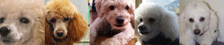
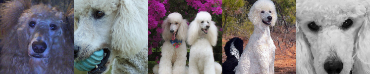
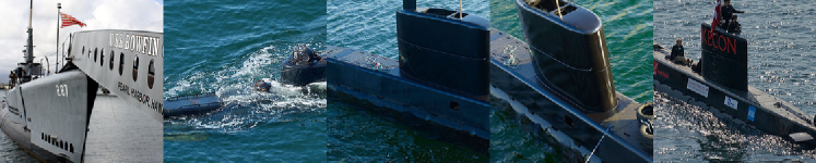
Figure L.1: We show 5 samples of miniature_poodle, standard_poodle and submarine classes in top, middle and bottom rows respectively. These samples are obtained from the ImageNet-1K validation set (Deng et al., 2009). As one can observe miniature_poodle and standard_poodle are semantically similar (They belong to the same category poodle). On the other hand submarine class is semantically dissimilar to both miniature_poodle and standard_poodle classes. We can clearly observe the systematic diffusion at increased $T$ in the presence of an LS-trained teacher for the semantically similar classes from the penultimate layer visualizations shown in Figures 1, A.1 and A.2.

In this section, we include samples images from 3 different classes used in the penultimate layer visualizations for ImageNet-1K and CUB200-2011 experiments. Refer to Figures L.1 and L.2 for ImageNet-1K and CUB200-2011 samples respectively.

Figure L.2: We show 5 samples of Great_grey_shrike, loggerhead_shrike and black_footed_albatross classes in top, middle and bottom rows respectively. These samples are obtained from the CUB200-2011 validation set (Wah et al., 2011). As one can observe Great_grey_shrike and loggerhead_shrike are semantically similar (They belong to the same category shrike). On the other hand black_footed_albatross class is semantically dissimilar to both Great_grey_shrike and loggerhead_shrike classes. We can clearly observe the systematic diffusion at increased $T$ in the presence of an LS-trained teacher for the semantically similar classes from the penultimate layer visualizations shown in Figures A.3, A.4 and A.5.

References

- Abbasi Koohpayegani et al. (2020) Abbasi Koohpayegani, S., Tejankar, A., and Pirsiavash, H. Compress: Self-supervised learning by compressing representations. Advances in Neural Information Processing Systems, 33:12980–12992, 2020.
- Arani et al. (2021) Arani, E., Sarfraz, F., and Zonooz, B. Noise as a resource for learning in knowledge distillation. In Proceedings of the IEEE/CVF Winter Conference on Applications of Computer Vision (WACV), pp. 3129–3138, January 2021.
- Chandrasegaran et al. (2021) Chandrasegaran, K., Tran, N.-T., and Cheung, N.-M. A closer look at fourier spectrum discrepancies for cnn-generated images detection. In Proceedings of the IEEE/CVF Conference on Computer Vision and Pattern Recognition (CVPR), pp. 7200–7209, June 2021.
- Chiu et al. (2018) Chiu, C.-C., Sainath, T. N., Wu, Y., Prabhavalkar, R., Nguyen, P., Chen, Z., Kannan, A., Weiss, R. J., Rao, K., Gonina, E., Jaitly, N., Li, B., Chorowski, J., and Bacchiani, M. State-of-the-art speech recognition with sequence-to-sequence models. In 2018 IEEE International Conference on Acoustics, Speech and Signal Processing (ICASSP), pp. 4774–4778, 2018. doi: 10.1109/ICASSP.2018.8462105.
- Chorowski & Jaitly (2017) Chorowski, J. and Jaitly, N. Towards better decoding and language model integration in sequence to sequence models. In Proc. Interspeech 2017, pp. 523–527, 2017. doi: 10.21437/Interspeech.2017-343. URL http://dx.doi.org/10.21437/Interspeech.2017-343.
- Deng et al. (2009) Deng, J., Dong, W., Socher, R., Li, L.-J., Li, K., and Fei-Fei, L. ImageNet: A Large-Scale Hierarchical Image Database. In CVPR09, 2009.
- Dzanic et al. (2020) Dzanic, T., Shah, K., and Witherden, F. Fourier spectrum discrepancies in deep network generated images. Advances in neural information processing systems, 33:3022–3032, 2020.
- Fang et al. (2021) Fang, Z., Wang, J., Wang, L., Zhang, L., Yang, Y., and Liu, Z. {SEED}: Self-supervised distillation for visual representation. In International Conference on Learning Representations, 2021. URL https://openreview.net/forum?id=AHm3dbp7D1D.
- Fellbaum (1998) Fellbaum, C. (ed.). WordNet: An Electronic Lexical Database. Language, Speech, and Communication. MIT Press, Cambridge, MA, 1998. ISBN 978-0-262-06197-1.
- Fu et al. (2020) Fu, Y., Chen, W., Wang, H., Li, H., Lin, Y., and Wang, Z. Autogan-distiller: searching to compress generative adversarial networks. In Proceedings of the 37th International Conference on Machine Learning, pp. 3292–3303, 2020.
- He et al. (2019) He, T., Zhang, Z., Zhang, H., Zhang, Z., Xie, J., and Li, M. Bag of tricks for image classification with convolutional neural networks. In Proceedings of the IEEE/CVF Conference on Computer Vision and Pattern Recognition (CVPR), June 2019.
- Heo et al. (2019) Heo, B., Kim, J., Yun, S., Park, H., Kwak, N., and Choi, J. Y. A comprehensive overhaul of feature distillation. In Proceedings of the IEEE/CVF International Conference on Computer Vision, pp. 1921–1930, 2019.
- Hinton et al. (2015) Hinton, G., Vinyals, O., and Dean, J. Distilling the knowledge in a neural network. In NIPS Deep Learning and Representation Learning Workshop, 2015. URL http://arxiv.org/abs/1503.02531.
- Hu et al. (2018) Hu, M., Peng, Y., Wei, F., Huang, Z., Li, D., Yang, N., and Zhou, M. Attention-guided answer distillation for machine reading comprehension. In Proceedings of the 2018 Conference on Empirical Methods in Natural Language Processing, pp. 2077–2086, Brussels, Belgium, October-November 2018. Association for Computational Linguistics. doi: 10.18653/v1/D18-1232. URL https://www.aclweb.org/anthology/D18-1232.
- Huang et al. (2019) Huang, Y., Cheng, Y., Bapna, A., Firat, O., Chen, D., Chen, M., Lee, H., Ngiam, J., Le, Q. V., Wu, Y., and Chen, z. Gpipe: Efficient training of giant neural networks using pipeline parallelism. In Wallach, H., Larochelle, H., Beygelzimer, A., d'Alché-Buc, F., Fox, E., and Garnett, R. (eds.), Advances in Neural Information Processing Systems, volume 32. Curran Associates, Inc., 2019. URL https://proceedings.neurips.cc/paper/2019/file/093f65e080a295f8076b1c5722a46aa2-Paper.pdf.
- Jiao et al. (2020) Jiao, X., Yin, Y., Shang, L., Jiang, X., Chen, X., Li, L., Wang, F., and Liu, Q. TinyBERT: Distilling BERT for natural language understanding. In Findings of the Association for Computational Linguistics: EMNLP 2020, pp. 4163–4174, Online, November 2020. Association for Computational Linguistics. doi: 10.18653/v1/2020.findings-emnlp.372. URL https://www.aclweb.org/anthology/2020.findings-emnlp.372.
- Khosla et al. (2020) Khosla, P., Teterwak, P., Wang, C., Sarna, A., Tian, Y., Isola, P., Maschinot, A., Liu, C., and Krishnan, D. Supervised contrastive learning. In Larochelle, H., Ranzato, M., Hadsell, R., Balcan, M. F., and Lin, H. (eds.), Advances in Neural Information Processing Systems, volume 33, pp. 18661–18673. Curran Associates, Inc., 2020. URL https://proceedings.neurips.cc/paper/2020/file/d89a66c7c80a29b1bdbab0f2a1a94af8-Paper.pdf.
- Kwon et al. (2020) Kwon, K., Na, H., Lee, H., and Kim, N. S. Adaptive knowledge distillation based on entropy. In ICASSP 2020 - 2020 IEEE International Conference on Acoustics, Speech and Signal Processing (ICASSP), pp. 7409–7413, 2020. doi: 10.1109/ICASSP40776.2020.9054698.
- Li et al. (2020a) Li, C., Peng, J., Yuan, L., Wang, G., Liang, X., Lin, L., and Chang, X. Block-wisely supervised neural architecture search with knowledge distillation. In Proceedings of the IEEE/CVF Conference on Computer Vision and Pattern Recognition, pp. 1989–1998, 2020a.
- Li et al. (2020b) Li, M., Lin, J., Ding, Y., Liu, Z., Zhu, J.-Y., and Han, S. Gan compression: Efficient architectures for interactive conditional gans. In Proceedings of the IEEE/CVF conference on computer vision and pattern recognition, pp. 5284–5294, 2020b.
- Lim et al. (2018) Lim, S. K., Loo, Y., Tran, N. T., Cheung, N. M., Roig, G., and Elovici, Y. Doping: Generative data augmentation for unsupervised anomaly detection with gan. In 18th IEEE International Conference on Data Mining, ICDM 2018, pp. 1122–1127. Institute of Electrical and Electronics Engineers Inc., 2018.
- Liu et al. (2022) Liu, Z., Mao, H., Wu, C.-Y., Feichtenhofer, C., Darrell, T., and Xie, S. A convnet for the 2020s. In Proceedings of the IEEE/CVF Conference on Computer Vision and Pattern Recognition, pp. 11976–11986, 2022.
- Lopez-Paz et al. (2016) Lopez-Paz, D., Schölkopf, B., Bottou, L., and Vapnik, V. Unifying distillation and privileged information. In International Conference on Learning Representations (ICLR), November 2016.
- Lukasik et al. (2020) Lukasik, M., Bhojanapalli, S., Menon, A., and Kumar, S. Does label smoothing mitigate label noise? In III, H. D. and Singh, A. (eds.), Proceedings of the 37th International Conference on Machine Learning, volume 119 of Proceedings of Machine Learning Research, pp. 6448–6458. PMLR, 13–18 Jul 2020. URL http://proceedings.mlr.press/v119/lukasik20a.html.
- Mghabbar & Ratnamogan (2020) Mghabbar, I. and Ratnamogan, P. Building a multi-domain neural machine translation model using knowledge distillation. In Giacomo, G. D., Catalá, A., Dilkina, B., Milano, M., Barro, S., Bugarín, A., and Lang, J. (eds.), ECAI 2020 - 24th European Conference on Artificial Intelligence, 29 August-8 September 2020, Santiago de Compostela, Spain, August 29 - September 8, 2020 - Including 10th Conference on Prestigious Applications of Artificial Intelligence (PAIS 2020), volume 325 of Frontiers in Artificial Intelligence and Applications, pp. 2116–2123. IOS Press, 2020. doi: 10.3233/FAIA200335. URL https://doi.org/10.3233/FAIA200335.
- Müller et al. (2019) Müller, R., Kornblith, S., and Hinton, G. E. When does label smoothing help? In Wallach, H., Larochelle, H., Beygelzimer, A., d'Alché-Buc, F., Fox, E., and Garnett, R. (eds.), Advances in Neural Information Processing Systems, volume 32. Curran Associates, Inc., 2019. URL https://proceedings.neurips.cc/paper/2019/file/f1748d6b0fd9d439f71450117eba2725-Paper.pdf.
- Nakashole & Flauger (2017) Nakashole, N. and Flauger, R. Knowledge distillation for bilingual dictionary induction. In Proceedings of the 2017 Conference on Empirical Methods in Natural Language Processing, pp. 2497–2506, Copenhagen, Denmark, September 2017. Association for Computational Linguistics. doi: 10.18653/v1/D17-1264. URL https://www.aclweb.org/anthology/D17-1264.
- Peng et al. (2019) Peng, Z., Li, Z., Zhang, J., Li, Y., Qi, G.-J., and Tang, J. Few-shot image recognition with knowledge transfer. In Proceedings of the IEEE/CVF International Conference on Computer Vision (ICCV), October 2019.
- Pereyra et al. (2017) Pereyra, G., Tucker, G., Chorowski, J., Kaiser, ., and Hinton, G. Regularizing neural networks by penalizing confident output distributions. 01 2017.
- Perez et al. (2020) Perez, A., Sanguineti, V., Morerio, P., and Murino, V. Audio-visual model distillation using acoustic images. In Proceedings of the IEEE/CVF Winter Conference on Applications of Computer Vision (WACV), March 2020.
- Real et al. (2019) Real, E., Aggarwal, A., Huang, Y., and Le, Q. V. Regularized evolution for image classifier architecture search. Proceedings of the AAAI Conference on Artificial Intelligence, 33(01):4780–4789, Jul. 2019. doi: 10.1609/aaai.v33i01.33014780. URL https://ojs.aaai.org/index.php/AAAI/article/view/4405.
- Sandler et al. (2018) Sandler, M., Howard, A., Zhu, M., Zhmoginov, A., and Chen, L.-C. Mobilenetv2: Inverted residuals and linear bottlenecks. In Proceedings of the IEEE conference on computer vision and pattern recognition, pp. 4510–4520, 2018.
- Shen et al. (2020) Shen, P., Lu, X., Li, S., and Kawai, H. Knowledge distillation-based representation learning for short-utterance spoken language identification. IEEE/ACM Transactions on Audio, Speech, and Language Processing, 28:2674–2683, 2020.
- Shen et al. (2021a) Shen, Z., Liu, Z., Liu, Z., Savvides, M., Darrell, T., and Xing, E. Un-mix: Rethinking image mixtures for unsupervised visual representation learning, 2021a.
- Shen et al. (2021b) Shen, Z., Liu, Z., Xu, D., Chen, Z., Cheng, K.-T., and Savvides, M. Is label smoothing truly incompatible with knowledge distillation: An empirical study. In International Conference on Learning Representations, 2021b. URL https://openreview.net/forum?id=PObuuGVrGaZ.
- Szegedy et al. (2016) Szegedy, C., Vanhoucke, V., Ioffe, S., Shlens, J., and Wojna, Z. Rethinking the inception architecture for computer vision. In IEEE Conference on Computer Vision and Pattern Recognition (CVPR), pp. 2818–2826, 2016. doi: 10.1109/CVPR.2016.308.
- Tan & Le (2019) Tan, M. and Le, Q. Efficientnet: Rethinking model scaling for convolutional neural networks. In International conference on machine learning, pp. 6105–6114. PMLR, 2019.
- Tang et al. (2021) Tang, J., Shivanna, R., Zhao, Z., Lin, D., Singh, A., Chi, E. H., and Jain, S. Understanding and improving knowledge distillation, 2021.
- Tran et al. (2021) Tran, N.-T., Tran, V.-H., Nguyen, N.-B., Nguyen, T.-K., and Cheung, N.-M. On data augmentation for gan training. IEEE Transactions on Image Processing, 30:1882–1897, 2021.
- Vaswani et al. (2017) Vaswani, A., Shazeer, N., Parmar, N., Uszkoreit, J., Jones, L., Gomez, A. N., Kaiser, L. u., and Polosukhin, I. Attention is all you need. In Guyon, I., Luxburg, U. V., Bengio, S., Wallach, H., Fergus, R., Vishwanathan, S., and Garnett, R. (eds.), Advances in Neural Information Processing Systems, volume 30. Curran Associates, Inc., 2017. URL https://proceedings.neurips.cc/paper/2017/file/3f5ee243547dee91fbd053c1c4a845aa-Paper.pdf.
- Wah et al. (2011) Wah, C., Branson, S., Welinder, P., Perona, P., and Belongie, S. The Caltech-UCSD Birds-200-2011 Dataset. Technical Report CNS-TR-2011-001, California Institute of Technology, 2011.
- Wang et al. (2021) Wang, D., Gong, C., Li, M., Liu, Q., and Chandra, V. Alphanet: Improved training of supernets with alpha-divergence. In Meila, M. and Zhang, T. (eds.), Proceedings of the 38th International Conference on Machine Learning, volume 139 of Proceedings of Machine Learning Research, pp. 10760–10771. PMLR, 18–24 Jul 2021. URL https://proceedings.mlr.press/v139/wang21i.html.
- Yu & Pool (2020) Yu, C. and Pool, J. Self-supervised generative adversarial compression. In Larochelle, H., Ranzato, M., Hadsell, R., Balcan, M., and Lin, H. (eds.), Advances in Neural Information Processing Systems, volume 33, pp. 8235–8246. Curran Associates, Inc., 2020. URL https://proceedings.neurips.cc/paper/2020/file/5d79099fcdf499f12b79770834c0164a-Paper.pdf.
- Yu et al. (2020) Yu, J., Jin, P., Liu, H., Bender, G., Kindermans, P.-J., Tan, M., Huang, T., Song, X., Pang, R., and Le, Q. Bignas: Scaling up neural architecture search with big single-stage models. In European Conference on Computer Vision, pp. 702–717. Springer, 2020.
- Yuan et al. (2020) Yuan, L., Tay, F. E., Li, G., Wang, T., and Feng, J. Revisiting knowledge distillation via label smoothing regularization. In IEEE/CVF Conference on Computer Vision and Pattern Recognition (CVPR), June 2020.
- Zhang et al. (2020) Zhang, M., Song, G., Zhou, H., and Liu, Y. Discriminability distillation in group representation learning. In Vedaldi, A., Bischof, H., Brox, T., and Frahm, J.-M. (eds.), Computer Vision – ECCV 2020, pp. 1–19, Cham, 2020. Springer International Publishing.
- Zoph et al. (2018) Zoph, B., Vasudevan, V., Shlens, J., and Le, Q. V. Learning transferable architectures for scalable image recognition. In 2018 IEEE/CVF Conference on Computer Vision and Pattern Recognition, pp. 8697–8710, 2018. doi: 10.1109/CVPR.2018.00907.