Particle creation in cosmological space-time
by a time-dependent electric field

Hadjar Rezki ^a,b and Slimane Zaim<sup>b*

a</sup>Laboratoire de Physique des Rayonnements et de leurs Intéractions avec la Matière

Département de Physique, Faculté des Sciences de la Matière

Université de Batna 1, Batna 05000, Algeria

^b Département de Physique , Faculté des Sciences de la Matière

Université de Batna 1, Batna 05000, Algeria

E-mail: zaim69slimane@yahoo.com (Corresponding author.*), h.rezki94@gmail.com

Abstract

In this work, we calculate the particle creation density in a cosmological anisotropic Bianchi I universe, by solving the Klein-Gordon and Dirac equations in the presence of a time-dependent electric field using the semi-classical method. We show that the particles distribution becomes thermal under the influence of the electric field when the electric interaction proportional to the Ricci scalar of curved space-time

Keywords: Cosmological space-time, Bogoliubov transformation, Particle production.

Pacs numbers: 11.10.Nx, 03.65.Pm, 03.70.+k , 25.75.Dw

1 Introduction

In the classical theory, black holes can only absorb and not emit particles. However, it was shown that quantum mechanical effects make black holes to create and emit particles. It is also well known that the most significant prediction of this theory is the phenomenon of particle creation which leads to the concept of quantum gravity. Particle creation phenomenon at the cost of gravitational field in the early universe has been studied extensively by Parker and al $\left[1-4\right]$. It follows that the study of quantum effects in cosmology becames a very attractive research field. However, only few attempts have been made to discuss these effects in the anisotropic universes $\left[1-4\right]$. It should be noted that when one studies the particles creation by the external fields, It should be no reasons to make distinction between the electromagnetic and the gravitational fields. In particular, it is possible to explain that the origin of matter in the universe is due to the transformation of the energy of the electromagnetic field into particles near the singularity. In order to study the mechanism of particle creation in cosmological backgrounds, there are several methods one can use such as adiabatic approach $[1,5]$, Feynman path integral method $[6]$, the Hamiltonian diagonalization technique $[7,8]$, as well as the Green function approach $[9]$.

In this research paper, we are interested on particles creaction by a non-stationary external electric field in non-static space-time using the semi-classical method, which is a well-posed problem in cosmology. There are technical difficulties one can encounter when treating the particle creation in time-dependent electromagnetic fields due to the limited number of simple models $[7]$. An interesting scenario for discussing particle creation process is the presence of a non-stationary electric field in Bianchi I anisotropic universe associated with the metric:

$$ds^{2}=-dt^{2}+t^{2}\left(dx^{2}+dy^{2}\right)+t^{-2}dz^{2}$$ (1)

Since the metric has a space-like singularity at $t=0$, it is difficult to define the particle states within the adiabatic approach [$1,5$]. To overcome this problem, we follow the quasi-classical approach. Firstly, we identify the positive and negative frequency modes by solving the classical Hamilton-Jacobi equation and look for the asymptotic behaviour of the solutions when $t\rightarrow 0$ and $t\rightarrow\infty$. Secondly, we solve the Klein-Gordon (K.G) and Dirac equations by comparing them with the above quasi-classical limits, then we identify the positive and negative frequency states. Thirdly, using the Bogoliubov transformations we compute the number density of the created particles. It turns out that in the quasi-classical limit, the positive and negative frequency modes have positive and negative eigenvalues, respectively.

The phenomenon of scalar and Dirac particles creation in an anisotropic Bianchi I universe with a constant and time-varying electric fields has been analyzed in refs.$\left[10-15\right]$. It is clear from these works that the particle distribution becomes thermal when one neglects the electrical interaction. Our objective is to study the creation of scalar and Dirac particles from vacuum in the space-time anisotropic Bianchi I universe and in the presence of a non-stationary electric field. From our results, the presence of the anisotropy with a non-stationary electric field lead to the creation of particles such that the distribution density becomes thermal under the influence of the electric field when it is proportional to the Ricci scalar curvature $R$.

This paper is organized as follows: In section 2, we solve the relativistic Hamilton-Jacobi equation and compute the quasi-classical energy modes. In section 3, we solve the K.G equation. Then, we compute the density of created scalar particles and discuss the weak and strong field limits. In section 4, we extend our study to solve the Dirac equation and obtain the density of the created Dirac particles. The last section is devoted to a discussion.

2 Hamilton Jacobi equation

The idea behind this method is as follows: We solve each of the Hamilton Jacobi equation, the K-G and Dirac equations for the Bianchi I space-time in the presence of a time-dependent electromagnetic field, then we compare the asymptotic behaviour of the solutions of the field equations and the Hamilton-Jacobi equation, at last identify the positive and negative frequency states. In the case of Hamilton-Jacobi method, the positive and negative frequency states are obtained according to the following

$$\varphi\left(\vec{x},t\right)=\exp\left(-iS\right),\text{ \ \ for positive frequency}$$ (2)

and

$$\varphi\left(\vec{x},t\right)=\exp\left(iS\right),\text{ \ \ for negative frequency}$$ (3)

where $S$ stands for the classical action.

The Hamilton Jacobi equation for the relativistic particle of rest mass $m$ and electric charge $e$ in an external vector field of vacuum is given by

$$g^{\mu\nu}\left(\frac{\partial S}{\partial x^{\mu}}+eA_{\mu}\right)\left(\frac{\partial S}{\partial x^{\nu}}+eA_{\nu}\right)+m^{2}=0$$ (4)

where $g^{\mu\nu}$ is a general inverse matrix of the tensor matrix $g_{\mu\nu}$ that is defined by the tetrad fields $e_{\mu}^{b}$ (which are a set of four space-time basis vectors) by the form

$$g_{\mu\nu}=e_{\mu}^{b}e_{\nu}^{a}\eta_{ba},\text{ \ \ }g^{\mu\nu}=e_{b}^{\mu}e_{a}^{\mu}\eta^{ba}$$ (5)

where $e$ is the electric charge, and $A_{\mu}$ is the electromagnetic four-potential. We note that here and elsewhere and for simplicity, we adopt the convention $c=1$ and $\hbar=1$.

By considering the cosmic scenario associated with the line element of the equation $(1)$, the metric tensor matrix $g$ is diagonalized as

$$g_{\mu\nu}=\left(\begin{array}[]{cccc}-1&0&0&0\\ 0&t^{2}&0&0\\ 0&0&t^{2}&0\\ 0&0&0&t^{-2}\end{array}\right)\qquad$$ (6)

with the inverse matrix $g^{\mu\nu}$

$$g^{\mu\nu}=\left(\begin{array}[]{cccc}-1&0&0&0\\ 0&t^{-2}&0&0\\ 0&0&t^{-2}&0\\ 0&0&0&t^{2}\end{array}\right)\qquad$$ (7)

For further simplifications, we consider a diagonal tetrad

$$e_{\mu}^{0} =\left(\begin{array}[]{cccc}1,&0,&0,&0\end{array}\right),$$ (9)

$$e_{\mu}^{1} =\left(\begin{array}[]{cccc}0,&t,&0,&0\end{array}\right),$$ (11)

$$e_{\mu}^{2} =\left(\begin{array}[]{cccc}0,&0,&t,&0\end{array}\right),$$ (13)

$$e_{\mu}^{3} =\left(\begin{array}[]{cccc}0,&0,&0,&t^{-1}\end{array}\right),$$ (15)

Moreover, the vector potential $A_{\mu}$ is chosen such that:

$$A_{\mu}=\left(0,0,0,\frac{\alpha}{t}+\frac{\beta}{t^{2}}\right),$$ (16)

which corresponds to a varying electric field along the $z$-direction, as the invariants appear

$$F_{\mu\nu}F^{\mu\nu}\neq 0\text{ \ and \ }F_{\mu\nu}^{\ast}F^{\mu\nu}=0$$ (17)

We note that there is no magnetic field here. Thus, the matrices of $g^{\mu\nu}$ and $A_{\mu}$ are only depending on time , and the $S$ function can be separated as

$$S=\vec{k}\cdot\vec{r}+F\left(t\right)$$ (18)

Substituting $(14)$ into $(4)$ we obtain the equation for the function $F\left(t\right)$

$$-\left(\frac{dF}{dt}\right)^{2}+\frac{k_{\perp}^{2}}{t^{2}}+t^{2}k_{z}^{2}+\left(ik_{z}t+e\alpha+\frac{e\beta}{t}\right)^{2}+m^{2}=0$$ (19)

where $k_{\perp}^{2}=k_{x}^{2}+k_{x}^{2}.$ For $k_{z}=0$ and $t\rightarrow 0$, the solution of equation $(15)$ is

$$F\left(t\right)=\pm\sqrt{k_{\perp}^{2}+e^{2}\beta^{2}}\log t$$ (20)

Hence , the wave function $\varphi\left(\vec{r},t\right)$ reads

$$\varphi\left(\vec{r},t\right)\sim\exp\left(i\vec{k}\cdot\vec{r}\right)t^{\pm\sqrt{k_{\perp}^{2}+e^{2}\beta^{2}}}$$ (21)

For $k_{z}=0$ and $t\rightarrow\infty$, the solution of equation $(15)$ is given by

$$F\left(t\right)=\pm\sqrt{m^{2}+e^{2}\alpha^{2}}t$$ (22)

Hence , the wave function $\varphi\left(\vec{r},t\right)$ reads

$$\varphi\left(\vec{r},t\right)\sim\exp\left(i\vec{k}\cdot\vec{r}\right)\exp\left(\pm\sqrt{m^{2}+e^{2}\alpha^{2}}t\right)$$ (23)

In order to determine the negative and positive frequency states of the scalar and Dirac particles, it is necessary to solve the K.G and Dirac equations in Bianchi I space-time in the presence of a time-dependent electric field.

3 Klein-Gordon equation and particle creation process

The simplest action for a massive scalar field in the presence of an electrodynamic gauge field $A_{\mu},$ for curved space-time is of the form

$$\mathcal{S}=\frac{1}{2}\int d^{4}x\text{ }(\Xi\left(g^{\mu\nu}\left(D_{\mu}\varphi\right)^{\dagger}D_{\nu}\varphi+\zeta R\varphi^{\dagger}\varphi+m^{2}\varphi^{\dagger}\varphi\right))\,,$$ (24)

where $\Xi=\det e_{\mu}^{b}$ is the Jacobian included to ensure that the action is a scalar under general coordinate transformations, and the gauge covariant derivative is defined as: $D_{\mu}\varphi=\left(\partial_{\mu}-ieA_{\mu}\right)\varphi$. The $R$ is the Ricci scalar, which has the form

$$R=g^{\mu\nu}R_{\mu\nu}$$ (25)

and it is defined by the Ricci tensor $R_{\mu\nu},$ which is of the form

$$R_{\mu\nu}=\partial_{\alpha}\Gamma_{\mu\nu}^{\alpha}-\partial_{\nu}\Gamma_{\mu\alpha}^{\alpha}+\Gamma_{\beta\alpha}^{\alpha}\Gamma_{\mu\nu}^{\beta}-\Gamma_{\mu\beta}^{\alpha}\Gamma_{\alpha\nu}^{\beta}$$ (26)

where  $\Gamma_{\mu\nu}^{\alpha}$ are the Christoffel symbols, defined by

$$\Gamma_{\mu\nu}^{\alpha}=\frac{1}{2}g^{\alpha\gamma}\left(\partial_{\nu}g_{\mu\gamma}+\partial_{\mu}g_{\gamma\nu}-\partial_{\gamma}g_{\mu\nu}\right)$$ (27)

Now, we use the infinitesimal generic field transformations ($\delta_{\lambda}\varphi=i\lambda\varphi$). We can prove that the action in eq. $\left(20\right)$ is actually invariant. By varying the scalar density under the gauge transformation, and from the generalised field equation and the Noether theorem, we obtain

$$\frac{\partial\mathcal{L}}{\partial\varphi}-\partial_{\mu}\frac{\partial\mathcal{L}}{\partial\left(\partial_{\mu}\varphi\right)}=0.$$ (28)

So the K.G equation in the curved space with the presence external field is given by

$$\left(-\square+m^{2}+\zeta R\right)\varphi=0$$ (29)

where

$$\square=\frac{1}{\Xi}D_{\mu}\left(\Xi e_{a}^{\mu}e^{\nu a}D_{\nu}\right)$$ (30)

and the scalar curvature $R$ is

$$R=2/t^{2}.$$ (31)

The determinant of the corresponding metric tensor $g_{\mu\nu}$ in eq.$(6)$ is

$$\Xi=\sqrt{\left|\det g\right|}=t$$ (32)

The line element $(1)$ has a singularity at $t=0$, consequently, the adiabatic approach $[1-5]$ cannot be applied in order to identify particle states. The standard method is to solve the Klein Gordon equation by comparing it with the quasi-classical limits, and specifying the positive and negative frequency states. Finally, by using the Bogoliubov transformations, one can obtain the number density for the created particles. The Klein-Gordon equation $\left(24\right)$ can be rewritten in the following simplified form

$$\left(g^{\mu\nu}\partial_{\mu}\partial_{\nu}-m^{2}-\xi R\right)\varphi\,-\left(ieg^{\mu\nu}\partial_{\mu}A_{\nu}+e^{2}g^{\mu\nu}A_{\mu}A_{\nu}+2ieg^{\mu\nu}A_{\mu}\partial_{\nu}\right)\varphi=0,$$ (33)

In this case, one can write

$$g^{\mu\nu}\partial_{\mu}\partial_{\nu}=-\partial_{0}^{2}-\frac{1}{t}\partial_{0}+\frac{1}{t^{2}}\left(\partial_{1}^{2}+\partial_{2}^{2}\right)+t^{2}\partial_{3}^{2},$$ (34)

and

$$2ieg^{\mu\nu}A_{\mu}\partial_{\nu}=2ie\left(\alpha t+\beta\right)\partial_{3},$$ (35)

and

$$e^{2}g^{\mu\nu}A_{\mu}A_{\nu}=\left[e\left(\alpha+\frac{\beta}{t}\right)\right]^{2}\,.$$ (36)

Then the Klein-Gordon equation $\left(29\right)$ is simplified to

$$\left[-\partial_{0}^{2}-\frac{1}{t}\partial_{0}+\frac{1}{t^{2}}\left(\partial_{1}^{2}+\partial_{2}^{2}\right)+t^{2}\partial_{3}^{2}-m^{2}-\xi R-2ie\left(\alpha t+\beta\right)\partial_{3}-e^{2}\left(\alpha+\frac{\beta}{t}\right)^{2}\right]\varphi=0.$$ (37)

Equation $\left(33\right)$ commutes with the operator $-i\overrightarrow{\nabla}$, therefore the wave function $\hat{\varphi}$ can be cast into

$$\varphi=t^{-1/2}w(t)\exp\left(ik_{x}x+ik_{y}y+ik_{z}z\right).$$ (38)

Substituting eq. $\left(34\right)$ into eq.$\left(33\right)$, one can get

$$\left[\frac{d^{2}}{dt^{2}}+\frac{k_{\bot}^{2}+e^{2}\beta^{2}+\frac{1}{4}+\xi}{t^{2}}+2\frac{e^{2}\alpha\beta}{t}+t^{2}k_{z}^{2}-2e\left(\alpha t+\beta\right)k_{z}+m^{2}+e^{2}\alpha^{2}\right]w(t)=0\,,$$ (39)

where the eigenvalue $k_{\bot}$ is given by

$$k_{\bot}=\sqrt{k_{x}^{2}+k_{y}^{2}}.$$ (40)

By adopting the following change of variable

$$\rho=-2i\sqrt{m^{2}+e^{2}\alpha^{2}}t,$$ (41)

We deduce that for $k_{z}=0,$ the equation $\left(35\right)$ becomes

$$\left[\frac{d^{2}}{d\rho^{2}}+\frac{\frac{1}{4}-\mu^{2}}{\rho^{2}}+\frac{\lambda}{\rho}-\frac{1}{4}\right]w(\rho)=0.$$ (42)

where

$$\mu\mathbf{=}i\sqrt{k_{\bot}^{2}+e^{2}\beta^{2}+2\xi}$$ (43)

and

$$\lambda=i\frac{e^{2}\alpha\beta}{\sqrt{m^{2}+e^{2}\alpha^{2}}}$$ (44)

The equation $(38)$ is the Whittaker differential equation $\left[16-18\right]$, therefore we can rewrite the solutions as a combination of Whittaker functions $M_{\tilde{k}_{\theta},\mu}\left(\rho\right)$ and $W_{\tilde{k}_{\theta},\mu}\left(\rho\right)$

$$w\left(\rho\right)=C_{1}M_{\lambda,\mathbf{\mu}}\left(\rho\right)+C_{2}W_{\lambda,\mathbf{\mu}}\left(\rho\right),$$ (45)

where $C_{1}$ and $C_{2}$ are normalisation constants, and the linear Whittaker functions $M_{\lambda,\mathbf{\mu}}\left(\rho\right)$ are

$$M_{\lambda,\mathbf{\mu}}\left(\rho\right)=\rho^{\mu+1/4}e^{-\rho/2}\left[1+\frac{\frac{1}{2}+\mu-\lambda}{1!\left(2\mu+1\right)}\rho+\frac{\left(\frac{1}{2}+\mu-\lambda\right)\left(\frac{31}{2}+\mu-\lambda\right)}{2!\left(2\mu+1\right)\left(2\mu+2\right)}\rho^{2}+........\right]$$ (46)

and

$$W_{\lambda,\mathbf{\mu}}\left(\rho\right)=\frac{\Gamma\left(-2\mu\right)}{\Gamma\left(\frac{1}{2}-\mu-\lambda\right)}M_{\lambda,\mathbf{\mu}}\left(\rho\right)+\frac{\Gamma\left(2\mu\right)}{\Gamma\left(\frac{1}{2}+\mu-\lambda\right)}M_{\lambda,-\mathbf{\mu}}\left(\rho\right)$$ (47)

We note that the Whittaker functions $M_{\lambda,\mathbf{\mu}}\left(\rho\right)$ and $W_{\lambda,\mathbf{\mu}}\left(\rho\right)$ have the following asymptotic limits:
for $\rho\rightarrow 0$

$$M_{\lambda,\mathbf{\mu}}\left(\rho\right) \sim \rho^{\mu+1/2}$$ (48)

$$W_{\lambda,\mathbf{\mu}}\left(\rho\right) \sim \frac{\Gamma\left(2\mu\right)}{\Gamma\left(\frac{1}{2}+\mu-\lambda\right)}\rho^{-\mu+1/2}$$ (49)

and for $\rho\rightarrow\infty$:

$$M_{\lambda,\mathbf{\mu}}\left(\rho\right) \sim \frac{\Gamma\left(2\mu\right)}{\Gamma\left(\frac{1}{2}+\mu-\lambda\right)}\rho^{-\lambda}\exp\left(\rho/2\right)$$ (50)

$$W_{\lambda,\mathbf{\mu}}\left(\rho\right) \sim \rho^{\lambda}\exp\left(-\rho/2\right)$$ (51)

To construct the positive and negative frequency modes, we use the asymptotic limit of the solution $\left(38\right)$ at $t=0$ $\left(\rho=0\right)$ and $t\rightarrow\infty$ . Thus, it may be shown that the positive and negative frequency modes are of the form

$$w_{0}^{+}=C_{0}^{+}M_{\lambda,\mathbf{\mu}}\left(\rho\right),$$ (52)

and

$$w_{0}^{-}=\left(w_{0}^{+}\right)^{\ast}=C_{0}^{+}\left(-1\right)^{-\mu+\frac{1}{2}}M_{\lambda,-\mathbf{\mu}}\left(\rho\right),$$ (53)

It is easy to find the positive and negative frequency modes for $\left|\rho\right|\rightarrow\infty$, by observing the asymptotic limit of $W_{\lambda,\mathbf{\mu}}\left(\rho\right)$, they are given by

$$w_{\infty}^{+}=C_{\infty}^{+}W_{\lambda,\mathbf{\mu}}\left(\rho\right),$$ (54)

and

$$w_{\infty}^{-}=C_{\infty}^{-}W_{-\lambda,\mathbf{\mu}}\left(-\rho\right),$$ (55)

where $C_{\infty}^{+}$ and $C_{\infty}^{-}$ are normalisation constants.
It can be exploit the fact that the positive frequency mode $w_{\infty}^{+}$ can be written in terms of the positive ($w_{0}^{+}$) and negative ($w_{0}^{-}$) frequency modes through the Bogoliubov transformation as

$$w_{\infty}^{+}=\alpha w_{0}^{+}+\beta w_{0}^{-},$$ (56)

According to the relation $(43)$, the equation $\left(52\right)$ can also be rewritten as follows

$$\left.C_{\infty}^{+}\frac{\Gamma\left(-2\mu\right)}{\Gamma\left(\frac{1}{2}-\mu-\lambda\right)}M_{\lambda,\mathbf{\mu}}\left(\rho\right)+C_{\infty}^{+}\frac{\Gamma\left(2\mu\right)}{\Gamma\left(\frac{1}{2}+\mu-\lambda\right)}M_{\lambda,-\mathbf{\mu}}\left(\rho\right)\right.$$

$$\left.=\alpha C_{0}^{+}M_{\lambda,\mathbf{\mu}}\left(\rho\right)+\beta C_{0}^{+}\left(-1\right)^{-\mu+\frac{1}{2}}M_{\lambda,-\mathbf{\mu}}\left(\rho\right)\right.$$ (57)

To find $\alpha$ and $\beta$, we have

$$\alpha=\frac{C_{\infty}^{+}\Gamma\left(-2\mu\right)}{C_{0}^{+}\Gamma\left(\frac{1}{2}-\lambda-\mu\right)},\qquad\beta=\frac{C_{\infty}^{+}\Gamma\left(2\mu\right)}{C_{0}^{+}\Gamma\left(\frac{1}{2}-\lambda+\mu\right)}\exp\left(i\pi\left(\mu-1/2\right)\right),$$ (58)

with

$$\frac{\left|\beta\right|^{2}}{\left|\alpha\right|^{2}}=\left|\frac{\Gamma\left(\frac{1}{2}-\lambda-\mu\right)}{\Gamma\left(\frac{1}{2}-\lambda+\mu\right)}\right|^{2}\exp\left(-2\pi\mu\right).$$ (59)

Using the property of the Gamma function

$$\left|\Gamma\left(\frac{1}{2}+i\rho\right)\right|^{2}=\frac{\pi}{\cosh\left(\pi\rho\right)},$$ (60)

and by the simplification, one gets

$$\frac{\left|\beta\right|^{2}}{\left|\alpha\right|^{2}}=\frac{1+\exp\left(-2\pi\left(\mu-\lambda\right)\right)}{1+\exp\left(2\pi\left(\mu+\lambda\right)\right)}.$$ (61)

The probability to create a single particle into mode $k$ from vacuum is then given by

$$P_{k}=\frac{\left|\beta\right|^{2}}{\left|\alpha\right|^{2}}=\frac{\cosh\left[\pi\left(-\lambda+\mu\right)\right]}{\cosh\left[\pi\left(\lambda_{\theta}+\mu\right)\right]}\exp\left(-2\pi\mu\right).$$ (62)

Now, we need to calculate the density of the particles created $n_{k}$ by the effect of time-dependent electric field. For this, we use eq. $\left(52\right)$ so that

$$n_{k}=\left|\beta\right|^{2}\,.$$ (63)

where the Bogoliubov coefficients satisfy the relation

$$\text{ }\left|\alpha\right|^{2}-\left|\beta\right|^{2}=1\,,$$ (64)

Finally, the number density of the created particles reads

$$n_{k}=\frac{P_{k}}{1-P_{k}}=\exp\left[-\pi\left(\lambda+\mu\right)\right]\frac{\cosh\left[\pi\left(-\lambda+\mu\right)\right]}{\sinh\left(2\pi\mu\right)}\,.$$ (65)

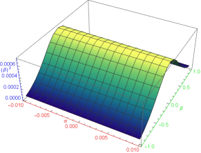
(a) {$\alpha,-0.01,0.01$},{ $\beta,-1,1$}

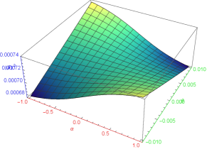
(b) {$\beta,-0.01,0.01$}, {$\alpha,-1,1$}

Figure 1: The number density of created KG particles as a function of $\alpha$ and $\beta$.

It is also worth considering the phenomenon of weak and strong electric field depend on the two parameters $\alpha$ and $\beta$, looking the behavior of number density and deriving some related thermodynamic quantities: Firstly, we assume that $\alpha=0$ , $\beta\neq 0,$ and the parameter $\lambda$ is zero, then the density of the created particles $(61)$ is of the form

$$n_{k}=\frac{1}{\exp\left[2\pi\left(\sqrt{k_{\bot}^{2}+2\xi+e^{2}\beta^{2}}\right)\right]-1}$$ (66)

This density is thermal and it looks like a two-dimensional Bose-Einstein distribution. For very weak electric fields the Eq. $(62)$ reduces to

$$n_{k}=\frac{1}{\exp\left[2\pi\sqrt{k_{\bot}^{2}+2\xi}+\pi\frac{e^{2}\beta^{2}}{\sqrt{k_{\bot}^{2}+2\xi}}\right]-1}$$ (67)

Equation $(61)$ indicates the presence of contribution of weak electric fields to particle creation with a chemical potential proportional to $\frac{e^{2}\beta^{2}}{\sqrt{k_{\bot}^{2}+2\xi}}$ . When $\beta\rightarrow 0$, the particle production $(63)$ becomes thermal:

$$n_{k}=\frac{1}{\exp\left[2\pi\sqrt{k_{\bot}^{2}+2\xi}\right]-1}$$

This expression shows that the density of the created particles is a Bose-Einstein distribution, with the absence of an electric field, and it is consistent with the results of refs $\left[11,19\right]$.
For very strong electric fields the Eq. $(62)$ reduces to

$$n_{k}\sim\exp\left[-\pi\frac{k_{\bot}^{2}+2\xi}{e\beta}-2\pi e\beta\right]$$ (68)

The expression $(64)$ corresponds to a thermal distribution with chemical potential proportional to $e\beta$. When $\beta\rightarrow\infty$, the particle production vanishes.
Secondly, we assume that $\alpha\neq 0$ and $\beta=0$, the density of created particles $(61)$ is of the form

$$n_{k}=\frac{1}{\exp\left[2\pi\sqrt{k_{\bot}^{2}+2\xi}\right]-1}$$ (69)

This expression shows that the density of the created particles is a Bose-Einstein distribution,it is the same as the result obtained in the absence of an electric field $\left[19\right].$

From the expression $(61)$, we observe that in the presence of the electric field $(12)$, the created particles distribution is not thermal and it depends on the effect of the electric field, but if the electric field is proportional to a scalar curvature of space-time, then the created particles is a Bose-Einstein distribution. One can see, of course, if $m=0$ , the equation $(33)$ describes the massless scalar particle in the Bianchi I space-time. The number of produced particles in this limit is given by

$$n_{k}=\frac{\exp\left[2\pi\left(\sqrt{k_{\bot}^{2}+2\xi+e^{2}\beta^{2}}-e\beta\right)\right]+1}{\exp\left[4\pi\left(\sqrt{k_{\bot}^{2}+2\xi+e^{2}\beta^{2}}\right)\right]-1}$$ (70)

This is consistent, whereas, according to quantum field theory, there are particles which are created from the energy of the electromagnetic field.
The quantity $\varepsilon_{k}=\sqrt{k_{\bot}^{2}+2\xi+e^{2}\beta^{2}}$ represents the energy, when we have the limit given by $\varepsilon_{k}\gg e\beta$, the particle spectrum in equation $(66)$ approximates to

$$n_{k}=\frac{1}{\exp\left(2\pi\varepsilon_{k}\right)-1}\sim\frac{1}{\exp\left(\frac{2\pi}{e\beta}\sqrt{k_{\bot}^{2}+2\xi}\right)-1}$$ (71)

which corresponds to a Planckian distribution with temperature $T=e\beta/\left(2\pi\right).$ The fact that the thermal spectrum can be generated from an electric field depends on time and the results are possible under certain conditions. It is a confirmation to explain that the origin of matter in the universe is due to the transformation of the energy of the electromagnetic field into particles near the singularity.

3.1 Dirac equation and particle creation process

In order to compute the density of created Dirac particles, we proceed to solve the Dirac equation in the cosmological background $(1)$ in the presence of the electric field $(12)$. The simplest action for a massive field spinors in the presence of an electrodynamic gauge field $A_{\mu},$ for the curved space-time is of the form

$$\mathcal{S}=\frac{1}{2}\int d^{4}xe\text{ }(i\left(\bar{\Psi}\tilde{D}\Psi-\overline{\tilde{D}\Psi}\Psi\right)-m\bar{\Psi}\Psi)\,,$$ (72)

Using the field equation $(24)$, with the generic field $\bar{\Psi}$ one can find in the co-moving frame the following Dirac equation

$$\left(\tilde{D}-m\right)\Psi=0$$ (73)

with

$$\tilde{D}=\tilde{\gamma}^{\mu}\left(\partial_{\mu}-\Gamma_{\mu}-ieA_{\mu}\right)$$ (74)

where the curved matrices $\tilde{\gamma}^{\mu}=e_{a}^{\mu}\gamma^{a}$  , ($\gamma^{a}$ represent the Minkowski Dirac matrices), satisfy the Clifford algebra

$$\left\{\tilde{\gamma}^{\mu},\tilde{\gamma}^{\nu}\right\}=2g^{\mu\nu}$$ (75)

and the spin connection $\Gamma_{\mu}$ is defined as

$$\Gamma_{\mu}=\frac{1}{4}\tilde{\gamma}^{\nu}\left(\partial_{\mu}\tilde{\gamma}_{\nu}-\Gamma_{\mu\nu}^{\alpha}\tilde{\gamma}_{\alpha}\right)$$ (76)

Then, the non zero componants of spin connections are

$$\Gamma_{1}=\frac{1}{2}\gamma^{0}\gamma^{1},\Gamma_{2}=\frac{1}{2}\gamma^{0}\gamma^{2},\Gamma_{3}=-\frac{1}{2t^{2}}\gamma^{0}\gamma^{3}$$ (77)

The Dirac equation $(69)$ takes the form

$$\left[\gamma^{0}\partial_{0}+\frac{1}{t}\left(\gamma^{1}\partial_{1}+\gamma^{2}\partial_{2}\right)+\gamma^{3}\left(t\partial_{3}-ie\alpha-\frac{ie\beta}{t}\right)-m\right]\Phi=0$$ (78)

where

$$\Psi=t^{-1/2}\Phi$$ (79)

It is important to mention that eq.$(74)$ can be rewritten as a sum of two first order differential equations as follows

$$\left\{t\left[\gamma^{3}\partial_{0}+\gamma^{0}\left(t\partial_{3}-ie\alpha-\frac{ie\beta}{t}\right)-m\gamma^{3}\gamma^{0}\right]+\left(\gamma^{1}\partial_{1}+\gamma^{2}\partial_{2}\right)\gamma^{3}\gamma^{0}\right\}\gamma^{3}\gamma^{0}\Phi=0$$ (80)

this equation $(76)$ can be rewritten in the form of operators as

$$\left\{K_{1}+K_{2}\right\}\phi=0$$ (81)

with

$$K_{2}\phi=k\phi=-K_{1}\phi$$ (82)

where

$$\phi=\gamma^{3}\gamma^{0}\Phi$$ (83)

The operators $K_{1}$ and $K_{2}$ have the expressions

$$K_{1} = t\left[\gamma^{3}\partial_{0}+\gamma^{0}\left(t\partial_{3}-ie\alpha-\frac{ie\beta}{t}\right)-m\gamma^{3}\gamma^{0}\right]$$ (84)

$$K_{2} = \left(\gamma^{1}\partial_{1}+\gamma^{2}\partial_{2}\right)\gamma^{3}\gamma^{0}$$ (85)

where $k$ is the separation constant. The spinor $\phi$ can be written as

$$\phi=\phi_{0}\exp\left(\vec{k}.\vec{r}\right)$$ (86)

Where $\phi_{0}$ is a bispinor as a function of $t$. Working in the representation where the Dirac matrices in the Minkowski space-time are given by

$$\gamma^{0}=\left(\begin{array}[]{cc}-i\sigma^{1}&0\\ 0&i\sigma^{1}\end{array}\right),\gamma^{1}=\left(\begin{array}[]{cc}0&i\\ -i&0\end{array}\right),\gamma^{2}=\left(\begin{array}[]{cc}\sigma^{2}&0\\ 0&-\sigma^{2}\end{array}\right),\gamma^{3}=\left(\begin{array}[]{cc}\sigma^{3}&0\\ 0&-\sigma^{3}\end{array}\right)$$ (87)

and the $\sigma_{i}$ ’s denote the $2\times 2$ Pauli matrices, we deduce that eq.$(78)$ is simplified to algebraic equations that permit to determine the relation between the components of the bispinor $\phi_{0}$ such as

$$\phi_{0}=\left(\begin{array}[]{c}\phi_{1}\\ \phi_{2}\end{array}\right)=\left(\begin{array}[]{c}\phi_{1}\\ \sigma_{2}\frac{k_{x}}{ik_{y}+k}\phi_{1}\end{array}\right)$$ (88)

where the eigenvalue $k$ is given by

$$k=i\sqrt{k_{x}^{2}+k_{y}^{2}}=ik_{\perp}$$ (89)

By using the representation in eq.$(83)$ and taking into account the spinor structure of eq.$(84)$, we deduce that for $k_{z}=0$, eq.$(76)$ is reduced to the following coupled system of first order differential equations

$$\left[\sigma^{3}\frac{d}{dt}+\sigma^{1}\left(e\alpha+\frac{e\beta}{t}\right)-m\sigma^{2}+\frac{k}{t}\right]\phi_{1} = 0$$ (90)

$$\left[-\sigma^{3}\frac{d}{dt}-\sigma^{1}\left(e\alpha+\frac{e\beta}{t}\right)-m\sigma^{2}+\frac{k}{t}\right]\phi_{2} = 0$$ (91)

It is easy to show that the eq. $(87)$ is equivalent to eq. $(86)$. Consequently, we have reduced the problem of solving eq. $(74)$ to find the solution of eq.$(86)$. The eq.$(86)$, after multiplying it from the right in $\sigma^{3}$, takes the following form

$$\left[\partial_{0}+i\sigma^{2}\left(e\alpha-e\frac{\beta}{t}\right)+im\sigma^{1}+\sigma^{3}\frac{k}{t}\right]\Phi_{1}=0$$ (92)

In order to solve $(88)$, we use the linear transformation $T$  $[20]$

$$T=\left(\begin{array}[]{cc}a&-b\\ a&b\end{array}\right)$$ (93)

where $a$ and $b$ are non zero arbitrary constants. After the act of the transformation $T$, the equation $(88)$ is written as

$$\left[\partial_{0}+iT\sigma^{2}T^{-1}\left(e\alpha-e\frac{\beta}{t}\right)+imT\sigma^{1}T^{-1}+T\sigma^{3}T^{-1}\frac{k}{t}\right]T\Phi_{1}=0$$ (94)

Where the matrix transformation $(89)$ acts on the $\sigma^{i}$ as follows

$$T\sigma^{1}T^{-1} = \frac{1}{2ab}\left(\begin{array}[]{cc}-a^{2}-b^{2}&a^{2}-b^{2}\\ -a^{2}+b^{2}&a^{2}+b^{2}\end{array}\right)$$ (97)

$$iT\sigma^{2}T^{-1} = \frac{1}{2ab}\left(\begin{array}[]{cc}-a^{2}+b^{2}&a^{2}+b^{2}\\ -a^{2}-b^{2}&a^{2}-b^{2}\end{array}\right)$$ (100)

$$T\sigma^{3}T^{-1} = \left(\begin{array}[]{cc}0&1\\ 1&0\end{array}\right)=\sigma^{1}$$ (103)

and

$$T\Phi=\digamma=\left(\begin{array}[]{c}f_{1}\\ f_{2}\end{array}\right)$$ (104)

Now, substituting $(92)$ and $\left(91\right)$ into $(90)$, we find the system of equations

$$\left.\rho\frac{df_{1}}{d\rho}+\left[\left(\frac{e\alpha}{4a^{2}b^{2}}\rho-\frac{e\beta}{2ab}\right)\left(-a^{2}+b^{2}\right)-im\frac{b^{2}+a^{2}}{4a^{2}b^{2}}\rho\right]f_{1}+\right.$$

$$\left.\left[\left(\frac{e\alpha}{4a^{2}b^{2}}\rho-\frac{e\beta}{2ab}\right)\left(a^{2}+b^{2}\right)\right.\left.-\left.im\frac{b^{2}-a^{2}}{4a^{2}b^{2}}\rho+k\right]f_{2}=0\right.\right.$$ (105)

$$\left.\rho\frac{df_{2}}{d\rho}+\left[-\left(\frac{e\alpha}{4a^{2}b^{2}}\rho-\frac{e\beta}{2ab}\right)\left(a^{2}+b^{2}\right)+im\frac{b^{2}-a^{2}}{4a^{2}b^{2}}\rho+k\right]f_{1}+\right.$$

$$\left.\left[\left(\frac{e\alpha}{4a^{2}b^{2}}\rho-\frac{e\beta}{2ab}\right)\left(a^{2}-b^{2}\right)+im\frac{b^{2}+a^{2}}{4a^{2}b^{2}}\rho\right]f_{2}=0\right.$$ (106)

where

$$\rho=2abt$$ (107)

For the simplest Whittaker equations, we choose $a$ and $b$ such that

$$\frac{b^{2}-a^{2}}{2} = -e\alpha$$

$$\frac{b^{2}+a^{2}}{2} = -im$$ (108)

then the system of equations becomes

$$\rho\frac{df_{1}}{d\rho}+\left(\frac{1}{2}\rho+\frac{e^{2}\alpha\beta}{\sqrt{-m^{2}-e^{2}\alpha^{2}}}\right)f_{1}+\left(\frac{ime\beta}{\sqrt{-m^{2}-e^{2}\alpha^{2}}}+k\right)f_{2} = 0$$

$$\rho\frac{df_{2}}{d\rho}-\left(\frac{1}{2}\rho+\frac{e^{2}\alpha\beta}{\sqrt{-m^{2}-e^{2}\alpha^{2}}}\right)f_{2}-\left[\frac{ime\beta}{\sqrt{-m^{2}-e^{2}\alpha^{2}}}-k\right]f_{1} = 0$$ (109)

In this way, we have reduced the problem of solving eqs.$(88)$ to that of finding the solutions of eqs.$(97)$. From eqs.$(97)$, we obtain the second order differential equation

$$\frac{d^{2}f_{1}}{d\rho^{2}}+\frac{1}{\rho}\frac{df_{1}}{d\rho}+\frac{\sigma}{\rho}f_{1}-\frac{\nu^{2}}{\rho^{2}}f_{1}-\frac{1}{4}f_{1}=0$$ (110)

where

$$\sigma=\frac{1}{2}+i\frac{e^{2}\alpha\beta}{\sqrt{m^{2}+e^{2}\alpha^{2}}},\nu=i\sqrt{k_{\perp}^{2}+e^{2}\beta^{2}}$$ (111)

The wave function $f_{1}$ can be written as

$$f_{1}=\rho^{-1/2}\omega$$ (112)

and the eq.$(98)$ is reduced to

$$\frac{d^{2}\omega_{1}}{d\rho^{2}}+\left(\frac{\sigma}{\rho}+\frac{\frac{1}{4}-\nu^{2}}{\rho^{2}}-\frac{1}{4}\right)\omega=0$$ (113)

This equation is the Whittaker differential equation $[16-18]$, therefore we can written the solution as a combination of Whittaker functions $M_{\tilde{k}_{\theta},\mu}\left(\rho\right)$ and $W_{\tilde{k}_{\theta},\mu}\left(\rho\right)$

$$\omega\left(\rho\right)=C_{1}M_{\sigma,\mathbf{\nu}}\left(\rho\right)+C_{2}W_{\sigma,\mathbf{\nu}}\left(\rho\right),$$ (114)

The asymptotic behaviour of the solutions will define the positive and negative frequency states in $t\rightarrow 0$ and $t\rightarrow\infty$

$$f_{1}^{+}\left(t\rightarrow 0\right) = C_{0}^{+}\rho^{-1/2}M_{\sigma,\mathbf{\nu}}\left(\rho\right)$$ (115)

$$f_{1}^{-}\left(t\rightarrow 0\right) = \exp\left(\pi\left|\mathbf{\nu}\right|\right)C_{0}^{-}\rho^{-1/2}M_{\sigma,-\mathbf{\nu}}\left(\rho\right)$$ (116)

and

$$f_{1}^{+}\left(t\rightarrow\infty\right) = C_{\infty}^{+}\rho^{-1/2}W_{\sigma,\mathbf{\nu}}\left(\rho\right)$$ (117)

$$f_{1}^{-}\left(t\rightarrow\infty\right) = C_{\infty}^{-}\rho^{-1/2}W_{-\sigma,\mathbf{\nu}}\left(\rho\right)$$ (118)

where $C_{0}^{+},C_{0}^{-}$ and $C_{\infty}^{+},C_{\infty}^{-}$ are the normalisation constants. The density of created particles can be calculated using the Bogoliubov transformation

$$f_{1}^{+}\left(t\rightarrow\infty\right)=\alpha f_{1}^{+}\left(t\rightarrow 0\right)+\beta f_{1}^{-}\left(t\rightarrow 0\right)$$ (119)

Now, we use the relation

$$W_{\sigma,\mathbf{\nu}}\left(\rho\right)=\frac{\Gamma\left(-2\mathbf{\nu}\right)}{\Gamma\left(\frac{1}{2}-\sigma-\mathbf{\nu}\right)}M_{\sigma,\mathbf{\nu}}\left(\rho\right)+\frac{\Gamma\left(2\mathbf{\nu}\right)}{\Gamma\left(\frac{1}{2}-\sigma+\mathbf{\nu}\right)}M_{\sigma,-\mathbf{\nu}}\left(\rho\right)$$ (120)

to find that $\alpha$ and $\beta$ are

$$\alpha=\frac{C_{\infty}^{+}\Gamma\left(-2\mathbf{\nu}\right)}{C_{0}^{+}\Gamma\left(\frac{1}{2}-\sigma-\mathbf{\nu}\right)},\text{ \ \ \ }\beta=\exp\left(-\pi\left|\mathbf{\nu}\right|\right)\frac{C_{\infty}^{+}\Gamma\left(2\mathbf{\nu}\right)}{C_{0}^{-}\Gamma\left(\frac{1}{2}-\sigma+\mathbf{\nu}\right)}$$ (121)

Using the property of the Gamma function

$$\left|\Gamma\left(ix\right)\right|^{2}=\frac{1}{x\sin\pi x}$$ (122)

we obtain

$$\left|\frac{\beta}{\alpha}\right|^{2}=\exp\left(-2\pi\sqrt{k_{\perp}^{2}+e^{2}\beta^{2}}\right)\frac{\Theta_{-}\sinh\pi\Theta_{-}}{\Theta_{+}\sinh\pi\Theta_{+}}$$ (123)

where

$$\Theta_{\pm}=\sqrt{k_{\perp}^{2}+e^{2}\beta^{2}}\pm\frac{e^{2}\alpha\beta}{\sqrt{m^{2}+e^{2}\alpha^{2}}}$$ (124)

From Eq.$(111)$ and taking into account the normalization condition for Dirac particles

$$\left|\alpha\right|^{2}+\left|\beta\right|^{2}=1$$ (125)

we find that the density of created Dirac particles is

$$n_{k}^{D}=\left|\beta\right|^{2}=\frac{\exp\left(-2\pi\sqrt{k_{\perp}^{2}+e^{2}\beta^{2}}\right)\Theta_{-}\sinh\pi\Theta_{-}}{\exp\left(-2\pi\sqrt{k_{\perp}^{2}+e^{2}\beta^{2}}\right)\Theta_{-}\sinh\pi\Theta_{-}+\Theta_{+}\sinh\pi\Theta_{+}}$$ (126)

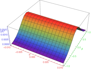
(a) {$\alpha,-0.01,0.01$},{ $\beta,-1,1$}

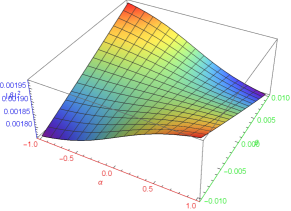
(b) {$\beta,-0.01,0.01$}, {$\alpha,-1,1$}

Figure 2: The number density of created Dirac particles as a function of $\alpha$ and $\beta$.

Let us discuss the special cases: the first one is when, $\alpha=0$ and $\beta\neq 0,$ the parameter $\Theta_{\pm}=\sqrt{k_{\perp}^{2}+e^{2}\beta^{2}}$ and the density of created particles $(114)$ is of the form

$$n_{k}^{D}=\frac{1}{\exp\left[2\pi\left(\sqrt{k_{\bot}^{2}+e^{2}\beta^{2}}\right)\right]+1}$$ (127)

This density is thermal and looks like a two-dimensional Fermi-Dirac distribution. In the case of strong electric fields, the number density of created Dirac particles takes the form

$$n_{k}^{D}\approx\exp\left[-\pi\frac{k_{\bot}^{2}}{e\beta}-2\pi e\beta\right]$$ (128)

The expression $(116)$ corresponds to a thermal distribution with chemical potential proportional to $e\beta.$
The second case is when, $\alpha\neq 0$ and $\beta=0$, the density of created particles $(114)$ is of the form

$$n_{k}^{D}=\frac{1}{\exp\left(2\pi k_{\bot}\right)+1}$$ (129)

This expression shows that the density of the created particles is a Fermi-Dirac distribution, it is the same result as in the absence of an electric field $\left[19\right].$

One can see, if $m=0$, the equation $(74)$ describes the massless Dirac particle in the Bianchi I space-time. The number density of produced particles in this limit is given by

$$n_{k}^{D}=\frac{\exp\left(-2\pi\varepsilon_{k}\right)\mathring{\Theta}_{-}\sinh\pi\mathring{\Theta}_{-}}{\exp\left(-2\pi\varepsilon_{k}\right)\mathring{\Theta}_{-}\sinh\pi\mathring{\Theta}_{-}+\mathring{\Theta}_{+}\sinh\pi\mathring{\Theta}_{+}}$$ (130)

where $\mathring{\Theta}=\varepsilon_{k}\pm e\beta$ and $\varepsilon_{k}=\sqrt{k_{\bot}^{2}+e^{2}\beta^{2}},$ when we have the limit given by $\varepsilon_{k}\gg e\beta$, the particle creation in equation $(118)$ approximates to

$$n_{k}^{D}=\frac{1}{\exp\left(2\pi\varepsilon_{k}\right)+1}\sim\frac{1}{\exp\left(\frac{2\pi}{e\beta}k_{\bot}\right)+1}$$ (131)

which corresponds to a Fermi-Dirac distribution with temperature $T=e\beta/\left(2\pi\right)$ and zero chemical potential, and which means that the expansion of the universe with a time-dependent electric field creates such particles thermally. Near the singularity, the origin of matter in the universe is due to the transformation of the electromagnetic field energy into particles.

4 Conclusions

In this paper, the obtained results show that the quasi-classical approach allows to calculate the density of created scalar and Dirac particles in non-static space-time with a non-stationary electromagnetic source.

In Figures $1$ and $2$, the dependence of created particles number density versus the electric field strength associated with the $\alpha$ and $\beta$ parameters is depicted. We have seen from the figures that the individual contributions of the first term of the electric field proportional to $t^{-1}$ and the second term proportional to $t^{-2}$ to the particle creation density can be useful physically for the electric fields proportional to $t^{-2}$, and the particle density becomes subject to Bose-Einstein and Fermi-Dirac thermal distributions. In the event that the second term of the electric field proportional to $t^{-2}$ vanishes, the electric fields proportional to $t^{-1}$ do not contribute to the number of created particles by the gravitational field.

So that the particle distribution becomes thermal only under the influence of the electric field when the electric interaction is proportional to the Ricci scalar of curved space-time. It was also confirmed that the origin of matter in the universe is due to the transformation of the the electromagnetic field energy into particles near the singularity.

References

[1] L. Parker, Phys. Rev.Lett. 21,562(1968).
[2] L. Parker, Phys. Rev. 183,1057(1969).
[3] L. Parker, Phys. Rev. D 3, 346 (1971).
[4] J. Papastamatiou and L. Parker, Phys. Rev. D 19, 2283 (1979).
[5] S. A. Fulling, Aspects of Quantum Field Theory in Curved
Space-Time (Cambridge University Press, Cambridge, 1991).
[6] D. M. Chitre and J. B. Hartle, Phys. Rev D 16, 251 (1977).
[7] A. A. Grib, S. G. Mamaev and V. M. Mostepanenko, Quantum Vacuum
Effects in Strong Fields (Energoatomizdat, Moscow, 1988).
[8] I. L. Bukhbinder, Izv. Vuzov. Fizika 7, 3 (1980).
[9] S. Gavrilov, D. M. Gitman, and S. D. Odintsov, Int. J. Mod.
Phys. A 12, 4837 (1997).
[10] Victor M. Villalba, International Journal of Theoretical
Physics, VoL 36, No. 6, 1997.
[11] V. M. Villalba, Phys. Rev. D 60 (1999) 127501.
[12] Victor M. Villalba, Walter Greiner, Phys. Rev. D65 (2002)
025007.
[13] V. M. Villalba and W. Greiner, Mod. Phys. Lett. A 17
(2002) 1883.
[14] N. Mebarki, L. Khodja, S. Zaim, EJTP 7, No. 23 (2010) 181–196.
[15] S. Zaim, Rom. Journ. Phys. Vol. 61, Nos. 5-6, P. 743-754,
(2016).
[16] N. N. Lebedev, Special Functions and their applications (New
York: Dover, 1972).
[17] M. Abramowitz and I. Stegun, Handbook of Mathematical Functions
(Dover, New York,1974).
[18] A Nikiforov, V. Ouvarov, Fonctions Spéciales de la Physique
Mathématique, Editions Mir, Moscou (1983).
[19] Pimentel, L.O., Pineda, F., Gen Relativ Gravit 53, 62 (2021).
[20] J. M. Cohen and B. Knharetz, J. Math. Phys. 34 (1993) 4964.