SPI-GAN: Distilling Score-based Generative Models with Straight-Path Interpolations

Abstract

Score-based generative models (SGMs) are a recently proposed paradigm for deep generative tasks and now show the state-of-the-art sampling performance. It is known that the original SGM design solves the two problems of the generative trilemma: i) sampling quality, and ii) sampling diversity. However, the last problem of the trilemma was not solved, i.e., their training/sampling complexity is notoriously high. To this end, distilling SGMs into simpler models, e.g., generative adversarial networks (GANs), is gathering much attention currently. We present an enhanced distillation method, called straight-path interpolation GAN (SPI-GAN), which can be compared to the state-of-the-art shortcut-based distillation method, called denoising diffusion GAN (DD-GAN). However, our method corresponds to an extreme method that does not use any intermediate shortcut information of the reverse SDE path, in which case DD-GAN fails to obtain good results. Nevertheless, our straight-path interpolation method greatly stabilizes the overall training process. As a result, SPI-GAN is one of the best models in terms of the sampling quality/diversity/time for CIFAR-10, CelebA-HQ-256, and LSUN-Church-256.

1 Introduction

Generative models are one of the most popular research topics for deep learning. There have been proposed many different models, ranging from variational autoencoders (VAEs) (Kingma and Welling, 2013) and generative adversarial networks (GANs) (Goodfellow et al., 2014) to recent score-based generative models (SGMs) (Song et al., 2021b, c).

Score matching with Langevin dynamics (SMLD) (Song and Ermon, 2019) and denoising diffusion probabilistic modeling (DDPM) (Ho et al., 2020) progressively corrupt original data and revert the corruption process to build a generative model. Recently, Song et al. (2021c) proposed a stochastic differential equation (SDE)-based mechanism that embraces all those models and coined the term, score-based generative models (SGMs).

Fig. 1 (a) shows the conceptual workflow of SGMs. The corruption process can be described by the forward SDE process with the Wiener process and the reverse SDE with a score function can be recognized as a generative model. It currently shows the state-of-the-art quality in synthesizing fake samples for various image datasets. However, one downside of this approach is large computational demands. To this end, some other variations to reduce the computational overheads have been recently proposed (Song and Ermon, 2020; San-Roman et al., 2021; Kong and Ping, 2021; Jolicoeur-Martineau et al., 2021a; Luhman and Luhman, 2021; Xiao et al., 2021b). Fig. 1 (b) (Xiao et al., 2021b) shows the key idea of one recent method that is the most similar to our research. Xiao et al. (2021b) proposed to approximate the reverse SDE process with $K$ shortcuts — their method is called as denoising diffusion GAN (DD-GAN) since they internally utilize a GAN-based architecture to learn the shortcuts. In other words, DD-GAN distills a target SGM to a GAN using the shortcuts. In contrast to DD-GAN, we propose to distill a target SGM using the straight-path interpolation (guided by intermediate samples by $t\mathbf{x}_{0}+(1-t)\mathbf{x}_{T}$, where $0\leq t\leq 1$). Our method is called straight-path interpolation GAN (SPI-GAN).

One may consider that SPI-GAN is similar to DD-GAN with $K=1$ (cf. Fig. 1 (b) vs. (c)). However, our SPI-GAN is technically different and more complicated in the following points:

1. Whereas DD-GAN uses the shortcuts following the SDE path, SPI-GAN uses the straight path between $\mathbf{x}_{T}$ and $\mathbf{x}_{0}$.

2. SPI-GAN utilizes interpolated samples, which can be written as $t\mathbf{x}_{0}+(1-t)\mathbf{x}_{T}$, where $0\leq t\leq 1$, to better approximate the straight path.

3. In order to learn from the interpolated samples, we propose i) a special neural network architecture, characterized by a mapping network, and ii) its own training mechanism. DD-GAN does not have a structure equivalent to our mapping network.

4. The mapping network in SPI-GAN utilizes neural ordinary differential equations (NODEs), which show good performance in processing sequences, and the generator of SPI-GAN generates samples following the straight path.

5. After all these efforts, SPI-GAN produces better outputs faster in comparison with not only existing distillation methods for SGMs, such as DD-GAN, but also other generative models.

Both DD-GAN and SPI-GAN can be understood as distillation methods from SGMs to GANs. However, our proposed SPI-GAN shows the best sampling quality and diversity overall in three benchmark datasets, CIFAR-10, CelebA-HQ-256, and LSUN-Church-256.

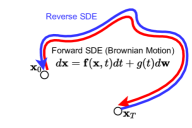
(a) The SDE-based workflow of SGMs. The reverse SDE is a generation process.

(b) Approximating the reverse SDE ($T$ steps in total) with $K$ shortcuts by DD-GAN, e.g., $K=3$ in this example.

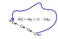
(c) Our proposed distillation method, SPI-GAN, with $K$ straight-path interpolations, e.g., $K=3$ in this example.

Figure 1: The comparison among three methods: i) the original formulation of SGMs in (a), ii) DD-GAN’s learning the shortcuts of the reverse SDE in (b), and iii) SPI-GAN’s learning the straight path in (c).

2 Related work and preliminaries

In diffusion models, the diffusion process is adding noise to real image data $\mathbf{x}_{0}\sim q(\mathbf{x}_{0})$ in $T$ steps as follows:

$${q(\mathbf{x}_{1:T}|\mathbf{x}_{0})=\prod_{t\geq 1}q(\mathbf{x}_{t}|\mathbf{x}_{t-1}),\quad q(\mathbf{x}_{t}|\mathbf{x}_{t-1})=\mathcal{N}(\mathbf{x}_{t};\sqrt{1-\beta_{t}}\mathbf{x}_{t-1},\beta_{t}\mathbf{I}),}$$ (1)

where $\beta_{t}$ is a pre-defined variance schedule and $q(\mathbf{x}_{0})$ is a data-generating distribution. The denoising (reverse) process of diffusion models is as follow:

$${p_{\boldsymbol{\theta}}(\mathbf{x}_{0:T})=p(\mathbf{x}_{T})\prod_{t\geq 1}p_{\boldsymbol{\theta}}(\mathbf{x}_{t-1}|\mathbf{x}_{t}),\quad p_{\boldsymbol{\theta}}(\mathbf{x}_{t-1}|\mathbf{x}_{t})=\mathcal{N}(\mathbf{x}_{t-1};\mu_{\boldsymbol{\theta}}(\mathbf{x}_{t},t),\sigma^{2}_{t}\mathbf{I}),}$$ (2)

which $\boldsymbol{\theta}$ is denoising model’s parameter, and $\mu_{\boldsymbol{\theta}}(\mathbf{x}_{t},t)$ and $\sigma^{2}_{t}$ are the mean and variance for the denoising model. Afterwards, score-based generative models (SGMs) generalize the diffusion process to continuous using SDE. SGMs use the following It$\hat{o}$ SDE to define diffusive processes:

$${d\mathbf{x}=f(\mathbf{x},t)dt+g(t)d\mathbf{w}},$$ (3)

where $\mathbf{w}$ is the standard Wiener process (a.k.a, Brownian motion), $f(\mathbf{x},t)$ and $g(t)$ are defined in Appendix A. Following the Eq. (3), we can derive a $\mathbf{x}_{t}$ at time $t\in[0,T]$. As the value of $t$ increases, $\mathbf{x}_{t}$ approaches to $\mathcal{N}(\mathbf{0},\boldsymbol{\sigma}^{2})$. The denoising process (reverse SDE) of SGMs is as follow:

$${d\mathbf{x}=[f(\mathbf{x},t)-g^{2}(t)\nabla{\mathbf{x}}\log p_{t}(\mathbf{x})]dt+g(t)d\mathbf{w}},$$ (4)

where $\nabla{\mathbf{x}}\log p_{t}(\mathbf{x})$ is the gradient of the log probability. In denoisng process (reverse SDE), a noisy sample at $t=T$ maps to a data sample at $t=0$.

Compared to other generative models, SGMs generate a variety of images with good quality. However, it takes a lot of time to generate the images. The reason is that a large $T$ (e.g., CIFAR-10: $T=1000$) is required to approximate $\mathbf{x}_{T}$ with a Gaussian distribution, and the image is generated through a large number of iterative time steps. To overcome slow sampling with large $T$, several methods have been proposed including learning an adaptive noise schedule (San-Roman et al., 2021), introducing non-Markovian diffusion processes (Song and Ermon, 2020; Kong and Ping, 2021), using faster SDE solvers for continuous-time models (Jolicoeur-Martineau et al., 2021a), knowledge distillation (Luhman and Luhman, 2021) and reducing denoising process steps (Xiao et al., 2021b).

Among those models, DD-GAN is the state-of-the-art model in terms of the sampling quality and time. They effectively reduce the denoising process steps. They argue that the denoising distribution, $p(\mathbf{x}_{t-1}|\mathbf{x}_{t})$, is a Gaussian distribution only when the time steps are large enough. Therefore, they reduce the denoising steps by learning a more complex and multimodal denoising distribution. They use GANs to learn complex distributions and iteratively generate images for $K$ steps ($K<T$). DD-GAN uses a conditional generator, and $\mathbf{x}_{t}$ is used as a condition to generate $\mathbf{x}_{t-1}$. Repeat this $K$ times to finally create $\mathbf{x}_{0}$. For its adversarial learning, the conditional GAN generator can match $p_{\boldsymbol{\theta}}(\mathbf{x}_{t-1}|\mathbf{x}_{t})$ and $q(\mathbf{x}_{t-1}|\mathbf{x}_{t})$.

DD-GAN is basically a distillation method for SGMs. The knowledge distillation (Buciluǎ et al., 2006; Hinton et al., 2015) is to train the knowledge of the teacher model which has high performing but expensive on a cheap model (student). It is also used in the diffusion model for fast sampling (Luhman and Luhman, 2021). They train the student model with the knowledge of mapping $\mathbf{x}_{T}$ to $\mathbf{x}_{0}$ without all the time steps of the teacher model. Therefore, they reduce the difference between $p_{teacher}(\mathbf{x}_{0}|\mathbf{x}_{T})$, the output distribution of the teacher model, and $p_{student}(\mathbf{x}_{0}|\mathbf{x}_{T})$, the output distribution of the student model, using only $\mathbf{x}_{T}$. Then, the student model, i.e., DD-GAN, can be trained with the knowledge of the teacher model, i.e., a target SGM model.

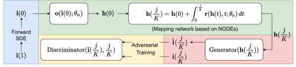
Figure 2: The overall architecture of our proposed SPI-GAN. We perform this adversarial training for $j\in(0,K]$. We set $\mathbf{i}(t)=t\mathbf{x}_{0}+(1-t)\mathbf{x}_{T}$, where $t=\frac{j}{K}$, and therefore, $\mathbf{i}(1)=\mathbf{x}_{0}$ and $\mathbf{i}(0)=\mathbf{x}_{T}$. We note that $\mathbf{i}(0)$ theoretically follows a certain Gaussian distribution $\mathcal{N}(\mathbf{0},\boldsymbol{\sigma}^{2})$, where $\boldsymbol{\sigma}^{2}$ depends on the type of SDE, and therefore, for generating fake images after finishing the distillation process we do not need $\mathbf{i}(0)$ from real images but $\mathbf{z}\sim\mathcal{N}(\mathbf{0},\boldsymbol{\sigma}^{2})$. Each color represents a computation step (cf. Sec. 3.1).

3 Proposed method

Our proposed method, SPI-GAN, distills a target SGM into a GAN. To this end, we rely on the straight interpolation path between $\mathbf{x}_{0}$ and $\mathbf{x}_{T}$. In this section, we describe our distillation method.

3.1 Overall workflow

We first describe the overall workflow of our proposed method. Before describing it, the notations in this paper are defined as follows: i) $\mathbf{i}(t)\in\mathbb{R}^{C\times H\times W}$ is an image with a channel $C$, a height $H$, and a width $W$ at interpolation point $t$. ii) $\hat{\mathbf{i}}(t)\in\mathbb{R}^{C\times H\times W}$ is a generated fake image at interpolation point $t$. iii) $\mathbf{h}(t)\in\mathbb{R}^{\dim(\mathbf{h})}$ is a latent vector at interpolation point $t$. iv) $\mathbf{r}(\mathbf{h}(t),t;\mathbf{\boldsymbol{\theta}}_{\mathbf{r}})\in\mathbb{R}^{\dim(\mathbf{h})}$ is a neural network approximating the time derivative of $\mathbf{h}(t)$, denoted $\frac{d\mathbf{h}(t)}{dt}$.

Our proposed SPI-GAN consists of four parts, each of which has a different color in Fig. 2, as follows:

1. 1st part (blue): The first part, highlighted in blue in Fig. 2, means that we calculate a noisy image $\mathbf{i}(0)=\mathbf{x}_{T}$ from $\mathbf{i}(1)=\mathbf{x}_{0}$ with the forward pass of the target SGM to distill. We note that this can be done in $\mathcal{O}(1)$.

2. 2nd part (green): The second part maps a noisy vector $\mathbf{i}(0)$ into another latent vector $\mathbf{h}(t)$, where $t=\frac{j}{K}$. We note that $t$ can be in $(0,1]$ to linearly interpolate $\mathbf{i}(0)$ and $\mathbf{i}(1)$. The final integral time of the NODE layer, denoted $\frac{j}{K}$, determines which latent vector it will generate.

3. 3rd part (red): The third part is a generative step to generate a fake image $\hat{\mathbf{i}}(t)$ from $\mathbf{h}(t)$. Our generator does not require $t$ as input, which means that $\mathbf{h}(t)$ internally has the temporal information. In other words, the latent space, where we sample $\mathbf{h}(t)$, is a common space across $t\in(0,1]$.

4. 4th part (yellow): The fourth part is a discriminative step to distinguish between real and fake images. We note that our discriminator reads, in conjunction with an image, its interpolation point $t$ to better distinguish. In other words, we maintain only one discriminator regardless of $t$.

5. The above adversarial training should be done with various values of $t\in(0,1]$. After that, our generator is able to generate fake images following the straight interpolation path.

3.2 Diffusion through the forward SDE

To distill a target SGM, SPI-GAN uses the forward SDE of the target model. Depending on the type of SDE, $\boldsymbol{\sigma}^{2}$ can be different for $\mathbf{i}(1)\sim\mathcal{N}(\mathbf{0},\boldsymbol{\sigma}^{2})$. In addition, we note that $\mathbf{i}(0)$ can be efficiently calculated from $\mathbf{i}(1)$, and its time complexity is $\mathcal{O}(1)$ given a fixed target model. Unlike the reverse SDE, which requires step-by-step computation, the forward SDE can be calculated with one-time computation for a target time $t$ (Song et al., 2021c).

We also note that the forward SDE computation can be done without its score network. The score network is needed to perform the reverse process. This is one more advantage of our distillation method. In some of existing distillation methods, e.g., DDPM Distillation (Luhman and Luhman, 2021), they first train the score network and then distill the reverse SDE. In our case, however, we use the straight interpolation path to distill a target SGM rather than the reverse SDE path. Therefore, we do not require any information from the reverse SDE path except its starting and ending images.

3.3 Mapping network

The mapping network which generates a latent vector $\mathbf{h}(t)$, where $t=\frac{j}{K}$, is the most important component in our model. We use a NODE-based mapping network to generate the latent vector for a target interpolation point $t$, whose initial value problem (IVP) is defined as follows:

$$\begin{split}{\mathbf{h}}\big{(}\frac{j}{K}\big{)}&=\mathbf{h}(0)+\int_{0}^{\frac{j}{K}}\mathbf{r}(\mathbf{h}(t),t;\mathbf{\boldsymbol{\theta}}_{\mathbf{r}})dt,\end{split}$$ (5)

where $\frac{d\mathbf{h}(t)}{dt}=\mathbf{r}(\mathbf{h}(t),t;\mathbf{\boldsymbol{\theta}}_{\mathbf{r}})$, and $\mathbf{r}$ has multiple fully-connected layers in our implementation. In addition, $\mathbf{h}(0)=\mathbf{o}(\mathbf{i}(0);\mathbf{\boldsymbol{\theta}}_{\mathbf{o}})$ — after training, we use $\mathbf{z}\sim\mathcal{N}(\mathbf{0},\boldsymbol{\sigma}^{2})$ instead of $\mathbf{i}(0)$ for generating various fake images. $\mathbf{o}$ is a network which generates the initial hidden representation from $\mathbf{i}(0)$ during training (or $\mathbf{z}$ during generating). In general, $\mathbf{h}(0)$ is a lower-dimensional representation of the input.

One more important point is that we maintain a single latent space for all $t$ and therefore, $\mathbf{h}(t)$ has the information of the image to generate at a target interpolation time $t$. For instance, Fig. 3 shows that a noisy image is generated from $\mathbf{h}(0)$ but a clean image from $\mathbf{h}(1)$. In Fig. 4, we also compare the reverse SDE path and the straight interpolation path. In general, the straight interpolation path more quickly converts a noisy image to its corresponding clear image than the reverse SDE path.

Figure 3: Process of generating sample from continuous latent vector

Figure 4: Difference between reverse SDE and interpolation

3.4 Generative adversarial network

SPI-GAN has advantages over traditional GANs. Since traditional GANs only generate clean fake images from noisy vectors, the overfitting issue occurs in the discriminator, which frequently results in mode-collapse at the end of the training process. However, our model is insensitive to the overfitting issue by generating a set of images following the straight interpolation path. The straight-path interpolation (SPI) method is defined as follows:

$$\mathbf{i}(t)=t\mathbf{x}_{0}+(1-t)\mathbf{x}_{T},$$ (6)

where $t=\frac{j}{K}$ and $j\in(0,K]$, and therefore, $\mathbf{i}(1)=\mathbf{x}_{0}$ and $\mathbf{i}(0)=\mathbf{x}_{T}$. If we use $K=3$, there are 3 interpolated images $\{\mathbf{i}(t_{k})\}_{k=1}^{3}$, where $t_{k}\in(0,1]$, $t_{k-1}<t_{k}$, and $t_{3}=1$, including the original image $\mathbf{i}(1)$. During our training process, we randomly sample $t_{k}$ rather than using a fixed interval of $\frac{1}{K}$ between $t_{k-1}$ and $t_{k}$, which increases the diversity of interpolated images.

3.4.1 Generator

Our generator is similar to that of StyleGAN2 (Karras et al., 2020b). Therefore, we borrow the network structure of StyleGAN2. However, the biggest difference from StyleGAN2 is that our mapping network has a continuous property and generates a latent vector at various interpolation points while maintaining one latent space across them. This is the key point in our model design to generate the interpolated image $\hat{\mathbf{i}}(t)$ with various $t$ settings. We refer to Appendix B.4 for the detailed network structure.

3.4.2 Discriminator

The discriminator of SPI-GAN is time-dependent, unlike the discriminator of traditional GANs. Therefore, we denote the discriminator as a mapping function Discriminator: $\mathbb{R}^{C\times H\times W}\times\mathbb{R}^{D}\xrightarrow{}[0,1]$, where $D$ is the dimension size of the time embedding. The discriminator receives $\hat{\mathbf{i}}(t)$ and the embedding of $t$ as input and learns to classify images from various interpolation points. As a result, it solves the overfitting problem that traditional GANs have since our discriminator sees various clean and noisy images. DD-GAN also uses this strategy to overcome the overfitting problem. As shown in Fig. 4, in addition, the straight-path interpolation method maintains a better balance between noisy and clean images than the case where we sample following the reverse SDE path. Therefore, our discriminator learns a more balanced set of noisy and clean images than that of DD-GAN. We refer to Appendix B.4 for the detailed network structure.

3.5 Training algorithm

Input: Training data $D_{train}$, Maximum iteration numbers $max\_iter$

1 Initialize $\mathbf{\boldsymbol{\theta}}$;

2

3$iter\leftarrow 0$;

4while $iter<max\_iter$ do

5       Create a mini-batch of real images $\{\mathbf{x}_{0}^{l}\}_{l=1}^{N}$, where $\mathbf{x}_{0}^{l}$ means $l$-th real image;

6       Calculate a mini-batch of noisy images $\{\mathbf{x}_{T}^{l}\}_{l=1}^{N}$ with the target forward SDE;

7       for $j\in\{j_{1},j_{2},\cdots,j_{K}\}$, where $j_{k}\sim\mathcal{U}(0,K)$, $j_{k-1}<j_{k}$, and $j_{K}=K$ do

8             Sample a set of noisy vectors $\{\mathbf{z}^{l}\}_{l=1}^{N}$, where $\mathbf{z}^{l}\sim\mathcal{N}(\mathbf{0},\boldsymbol{\sigma}^{2})$;

9             Calculate $\{\mathbf{h}^{l}(t)\}_{l=1}^{N}$, where $t=\frac{j}{K}$, with the mapping network which processes $\{(\mathbf{x}_{T}^{l},\mathbf{z}^{l})\}_{l=1}^{N}$;

10             Generate a fake image $\{\hat{\mathbf{i}}^{l}(t)\}_{l=1}^{N}$ with the generator;

11             Train the generator and the mapping network together;

12             Train the discriminator;

13            

14      $iter\leftarrow iter+1$;

15      

16return $\mathbf{\boldsymbol{\theta}}$;

Algorithm 1 How to train SPI-GAN

Our training algorithm is in Alg. (1). In each iteration, we first create a mini-batch of $N$ real images, denoted $\{\mathbf{x}_{0}^{l}\}_{l=1}^{N}$. Using the forward SDE of the target model to distill, we derive a mini-batch of $N$ noisy images, denoted $\{\mathbf{x}_{T}^{l}\}_{l=1}^{N}$. We then sample a set of values for $j\in\{j_{1},j_{2},\cdots,j_{K}\}$, where $j_{k}\sim\mathcal{U}(0,K)$, $j_{k-1}<j_{k}$, and $j_{K}=K$. Note that we randomly sample $\{j_{1},j_{2},\cdots,j_{K}\}$ from $(0,K]$ and the last value should be always $K$ (and therefore, $t=1$ in the last for-loop). After that, our mapping network generates a set of latent vectors, denoted $\{\mathbf{h}^{l}(t)\}_{l=1}^{N}$. Our generator then produces a set of fake images with the generated latent vectors. After that, we follow the standard adversarial training sequence, i.e., training the generator, followed by the discriminator.

Implementation Trick. We need to calculate $\mathbf{h}^{l}(t)$ for all $t=\frac{j}{K}$, where $j\in(0,K]$. However, we do not repeat the computation in Eq. (5) for each $j$, but incrementally solve the initial value problem from $j-1$ to $j$. In this way, we can minimize the overall computation.

3.6 How to generate

After finishing all the distillation processes, we need only the mapping network and the generator. After sampling $\mathbf{z}\sim\mathcal{N}(\mathbf{0},\boldsymbol{\sigma}^{2})$, we feed them into the mapping network to derive $\mathbf{h}(1)$ — we solve the initial value problem in Eq. (5) from 0 to 1 — and our generator generates a fake image $\hat{\mathbf{i}}(1)$.

4 Experiments

We describe our experimental environments and results. In Appendix B, more detailed experimental settings including software/hardware and hyperparameters, for reproducibility. We also release our model with trained checkpoints.

4.1 Experimental environments

Target models. Among various types, we distill SGMs based on the variance preserving SDE (VP-SDE) for their high sampling quality and reliability, which makes $\boldsymbol{\sigma}^{2}=1$. That is, $\mathbf{i}(1)$ and $\mathbf{z}$ follow a unit Gaussian distribution (see Appendix B.2 for more descriptions).

Datasets. We use CIFAR-10 (Krizhevsky et al., 2014), CelebA-HQ-256 (Karras et al., 2018), and LSUN-Church-256 (Yu et al., 2015). CIFAR-10 has a resolution of 32x32 and is one of the most widely used datasets. CelebA-HQ-256 and LSUN-Church-256 contain high-resolution images of 256x256. Each of them has many real-world images.

Evaluation metrics. We use 5 evaluation metrics to quantitatively evaluate fake images. The inception score (IS) (Salimans et al., 2016) and the Fréchet inception distance (FID) (Heusel et al., 2017) are traditional methods to evaluate the fidelity of fake samples. The improved recall (Recall) (Kynkäänniemi et al., 2019) reflects whether the variation of generated data matches the variation of training data. Finally, the number of function evaluations (NFE) and clock time (Time) are used to evaluate the generation time.

4.2 Main results

Table 1: Results of the unconditional generation on CIFAR-10

Model IS $\uparrow$ FID $\downarrow$ Recall$\uparrow$ NFE$\downarrow$ Time$\downarrow$ SPI-GAN (ours), K=2 10.3 3.09 0.66 1 0.04 Denoising Diffusion GAN (DD-GAN), K=4 (Xiao et al., 2021b) 9.63 3.75 0.57 4 0.21 DDPM (Ho et al., 2020) 9.46 3.21 0.57 1000 80.5 NCSN (Song and Ermon, 2019) 8.87 25.3 - 1000 107.9 Adversarial DSM (Jolicoeur-Martineau et al., 2021b) - 6.10 - 1000 - Likelihood SDE (Song et al., 2021b) - 2.87 - - - Score SDE (VE) (Song et al., 2021c) 9.89 2.20 0.59 2000 423.2 Score SDE (VP) (Song et al., 2021c) 9.68 2.41 0.59 2000 421.5 Probability Flow (VP) (Song et al., 2021c) 9.83 3.08 0.57 140 50.9 LSGM (Vahdat et al., 2021) 9.87 2.10 0.61 147 44.5 DDIM, T=50 (Song et al., 2021a) 8.78 4.67 0.53 50 4.01 FastDDPM, T=50 (Kong and Ping, 2021) 8.98 3.41 0.56 50 4.01 Recovery EBM (Gao et al., 2021) 8.30 9.58 - 180 - Improved DDPM (Nichol and Dhariwal, 2021) - 2.90 - 4000 - VDM (Kingma et al., 2021) - 4.00 - 1000 - UDM (Kim et al., 2021) 10.1 2.33 - 2000 - D3PMs (Austin et al., 2021) 8.56 7.34 - 1000 - Gotta Go Fast (Jolicoeur-Martineau et al., 2021a) - 2.44 - 180 - DDPM Distillation (Luhman and Luhman, 2021) 8.36 9.36 0.51 1 - SNGAN (Miyato et al., 2018) 8.22 21.7 0.44 1 - SNGAN+DGflow (Ansari et al., 2021) 9.35 9.62 0.48 25 1.98 AutoGAN (Gong et al., 2019) 8.60 12.4 0.46 1 - TransGAN (Jiang et al., 2021) 9.02 9.26 0.48 25 - StyleGAN2 w/o ADA (Karras et al., 2020b) 9.18 8.32 0.41 1 0.04 StyleGAN2 w/ ADA (Karras et al., 2020a) 9.83 2.92 0.49 1 0.04 StyleGAN2 w/ Diffaug (Zhao et al., 2020) 9.40 5.79 0.42 1 0.04 Glow (Kingma and Dhariwal, 2018) 3.92 48.9 - 1 - PicxelCNN (Van Oord et al., 2016) 4.60 65.9 - 1024 - NVAE (Vahdat and Kautz, 2020) 7.18 23.5 0.51 1 0.36 IGEBM (Du and Mordatch, 2019) 6.02 40.6 - 60 - VAEBM (Xiao et al., 2021a) 8.43 12.2 0.53 16 8.79

In this subsection, we evaluate our proposed model quantitatively and qualitatively. For CIFAR-10, we perform the unconditional image generation task for fair comparisons with existing models. The quantitative evaluation results are shown in Table LABEL:tbl:cifar10. Although our FID is 0.68 worse than that of the Score SDE (VP), it shows better scores in all other metrics. However, our method has a better FID score than that of DD-GAN, one of the most related methods. DD-GAN is inferior to our method for all those three quality metrics. LGSM also shows high quality for FID. However, its IS and recall scores are worse than ours. Our method’s sample generation time (Time) is almost the same as that of StyleGAN2, which is one of the fastest methods. In summary, SPI-GAN not only increases the quality of samples but also decreases the sampling time.

In addition, our model shows outstanding performance in all evaluation metrics compared to DD-GAN, the latest distillation model. In particular, SPI-GAN, unlike DD-GAN, does not increase the sample generation time even when $K$ is large — in fact, $K$ affects the training time of our method since for the generation, we always use $j=K$ regardless of how large/small $K$ is (cf. Sec. 3.6). Therefore, there is no trade-off between $K$ and the generation time, which is one good characteristic of our method.

Even for high-resolution images, our model shows good performance. In particular, our method shows the best FID score for CelebA-HQ-256 in Table 3, which shows the efficacy of our proposed distillation method. However, our method does not produce significant improvements for LSUN-Church-256 in Table LABEL:tbl:lsun — our method outperforms DD-GAN with other metrics in Table 5. The qualitative results are in Figs. 7, 7, and 7. As shown, our method is able to generate visually high-quality images. More detailed images are in Appendix C

Table 2: Results on CelebA-HQ-256

Model	FID$\downarrow$
SPI-GAN (ours)	6.62
DD-GAN	7.64
Score SDE	7.23
LSGM	7.22
UDM	7.16
NVAE	29.7
VAEBM	20.4
NCP-VAE (Aneja et al., 2021)	24.8
PGGAN (Karras et al., 2018)	8.03
Adv. LA (Pidhorskyi et al., 2020)	19.2
VQ-GAN (Esser et al., 2021b)	10.2
DC-AE (Parmar et al., 2021)	15.8

Table 3: Results on LSUN-Church-256

Model	FID$\downarrow$
SPI-GAN (ours)	6.03
DD-GAN	5.25
DDPM	7.89
ImageBART (Esser et al., 2021a)	7.32
Gotta Go Fast	25.6
PGGAN	6.42
StyleGAN (Karras et al., 2019)	4.21
StyleGAN2	3.86
CIPs (Anokhin et al., 2021)	2.92

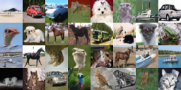
Figure 5: Qualitative results on CIFAR-10

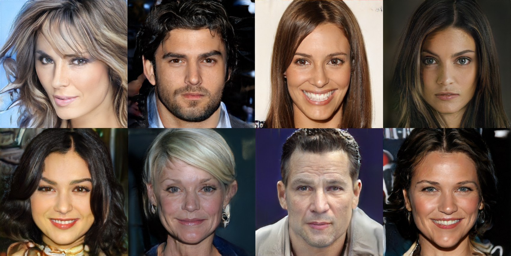
Figure 6: Qualitative results on CelebA-HQ-256

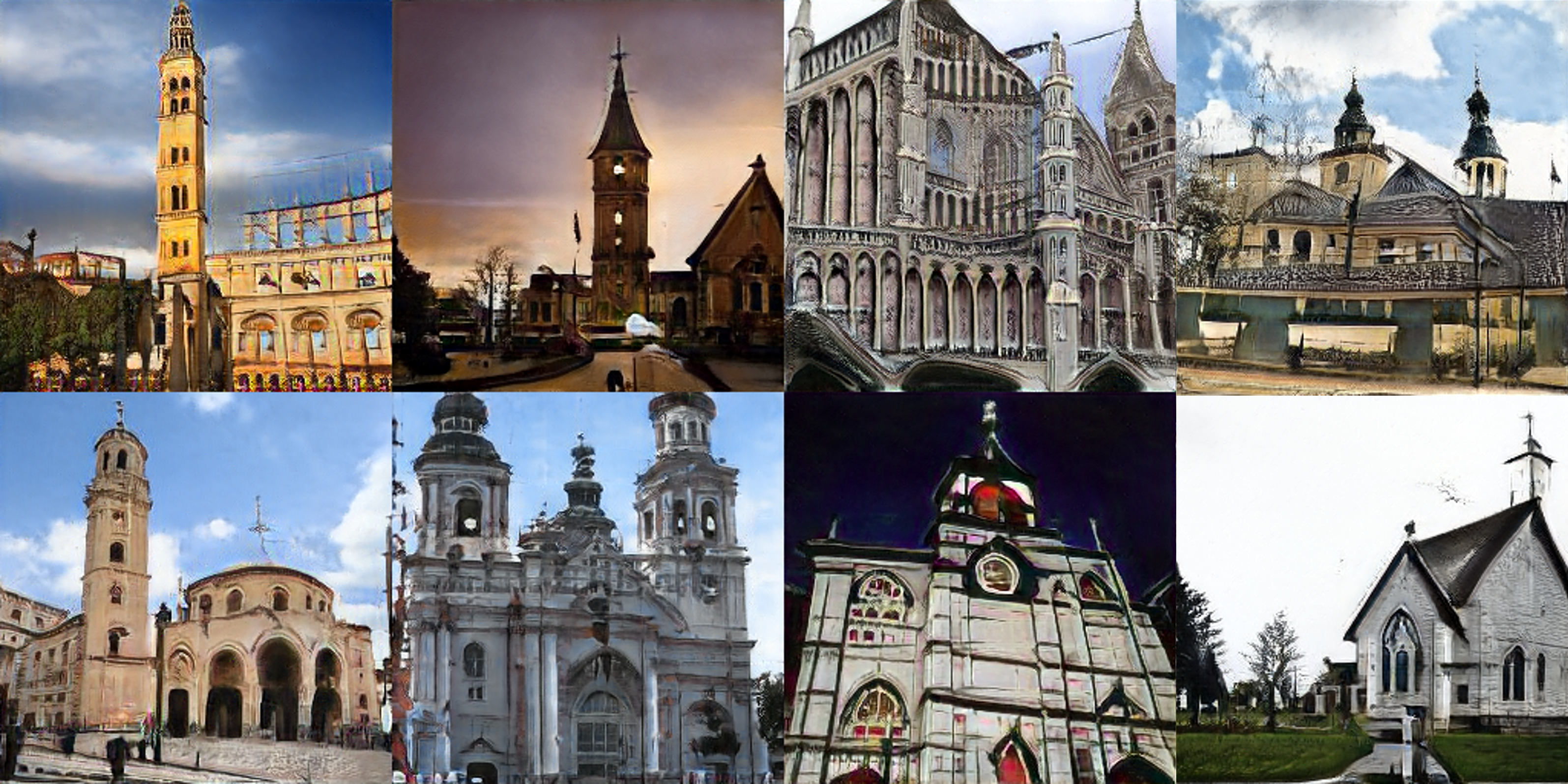
Figure 7: Qualitative results on LSUN-Church-256

4.3 Training time analyses

As clarified earlier, our method does not require training the target SGM to distill but its theoretical forward path equation is enough (for running the blue step in Fig. 2). For instance, therefore, our overall training consists of training our model only, which takes 6 days with 2 A6000 GPUs for CelebA-HQ-256. For training DD-GAN, it takes 6.5 days with 8 A100 GPUs. Training the original SGM model takes 10 days with 8 A100 GPUs. In comparison with them, our method is faster.

4.4 Ablation studies

In this subsection, we conduct experiments by changing i) the number of interpolations, $K$, or ii) fixing the intermediate points, $j=\{1,2,\cdots,K\}$, which are the two most important hyperparameters.

The number of interpolations. According to Table LABEL:tbl:ablation, the sampling fidelity, i.e., IS and FID, is the best when $K$=2, and Recall indicating the sampling diversity is the best when $K$=3. In general, the higher the value of $K$ is, the higher the sampling diversity is and the lower the sampling fidelity is. When $K$=1, the discriminator uses only clean images ($\textbf{i}(1)$) for learning. Comparison with DD-GAN ($K$=1) shows that our proposed model is more complicated than DD-GAN.

Fixed intermediate points. In our model, $j\sim\mathcal{U}(0,K)$ is stochastic between 0 and $K$. However, we can fix $j\in\{0,1,\dots,K\}$. That is, it does not learn about various $j$, but only train with a specific section (e.g., when $K=2$, $j\in\{0,1,2\}$). It can be seen that in Table LABEL:tbl:ablation and Fig. 8, however, our original stochastic setting not only shows better sampling quality than the fixed setting but also converges more rapidly.

Table 4: Ablation studies on CIFAR-10

Model	IS $\uparrow$	FID$\downarrow$	Recall$\uparrow$
$K$=1 (DD-GAN)	8.93	14.6	0.19
$K$=1 (SPI-GAN)	9.42	10.5	0.60
$K$=2	10.3	3.09	0.66
$K$=3	9.65	8.45	0.68
$K$=4	9.68	5.49	0.67
$K$=5	9.61	6.25	0.65
Fixed $j$	8.58	20.8	0.63

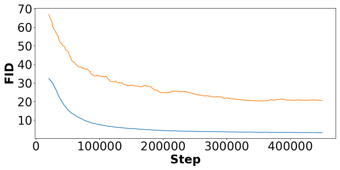
Figure 8: FID curves of the stochastic with $K=2$ (blue) vs. the fixed $j$ (orange)

4.5 Additional studies

We introduce additional results for evaluating sampling quality and interpolations.

Table 5: Improved quality metrics on LSUN-Church-256

Model	Recall$\uparrow$	Coverage$\uparrow$
SPI-GAN	0.28	0.65
DD-GAN	0.16	0.58
CIPs	0.43	0.57

Improved metrics. FID is one of the most popular evaluation metrics to measure the similarity between real and generated images. Generated images are sometimes evaluated for the fidelity and diversity using the improved precision and recall (Kynkäänniemi et al., 2019). However, the recall is not accurately detecting similarities between two distributions and is not robust against outliers. Therefore, we evaluate the generated images with the coverage (Naeem et al., 2020) which overcome the limitations of the recall. We compare our method with CIPs, which marks the best FID score in LSUN-Church-256, and the results are in Table 5. Our SPI-GAN outperforms CIPs in terms of the coverage.

Figure 9: Generation by varying the latent vector from $\mathbf{h}(0)$ to $\mathbf{h}(1)$ given fixed $\mathbf{z}$

Generation by manipulating $\mathbf{z}$ and $\mathbf{h}$. There are three manipulations parts in our model. The first one is generating by changing the latent vector from $\mathbf{h}(0)$ to $\mathbf{h}(1)$ in Fig. 9, the second one is the interpolation between two noisy vectors $\mathbf{z}^{\prime}$ and $\mathbf{z}^{\prime\prime}$ in Fig. 11, and the last one is the interpolation between two latent vector $\mathbf{h}(1)^{\prime}$ to $\mathbf{h}(1)^{\prime\prime}$ in Fig. 11. In Fig. 9, the ideal generation is that noises are gradually removed for an image, but similar images, not the same, are produced. However, the denoising patterns can be observed well. Figs. 11 and 11 show the interpolation of the noise vector (z) and the latent vector ($\mathbf{h}(1)$). One can observe that generated images are gradually changed from a mode to another.

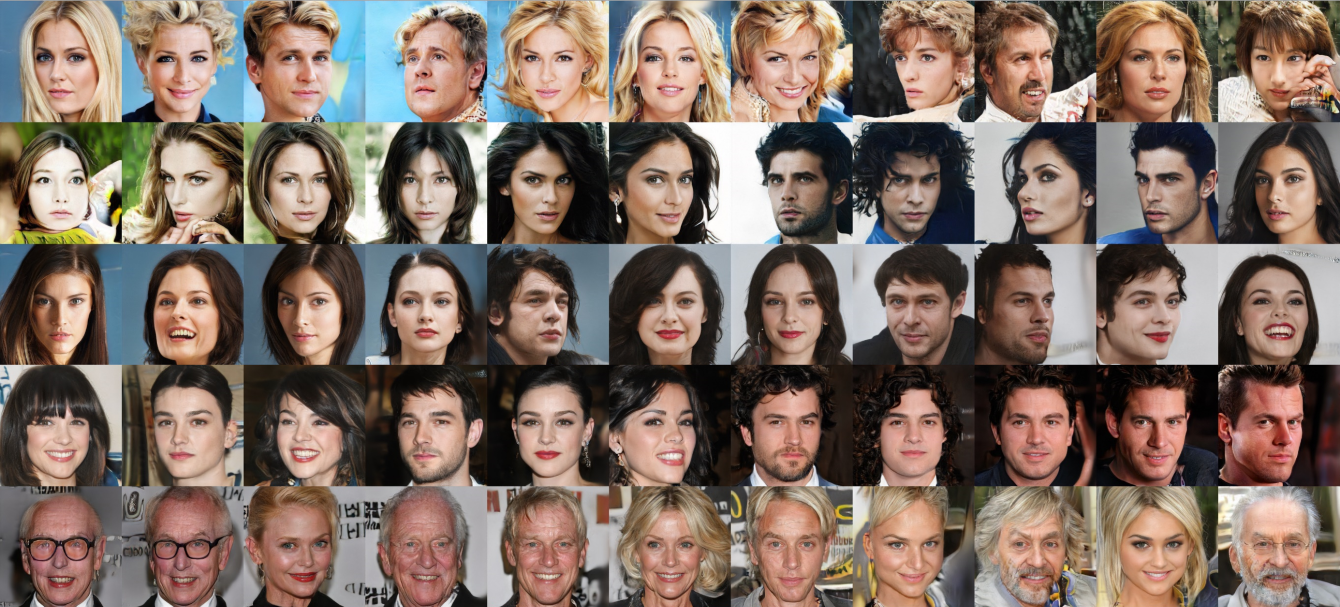
Figure 10: Generation by interpolating $\mathbf{z}=\\ (1-a)\mathbf{z}^{\prime}+a\mathbf{z}^{\prime\prime}$

Figure 11: Generation by interpolating $\mathbf{h}(1)=\\ (1-a)\mathbf{h}(1)^{\prime}+a\mathbf{h}(1)^{\prime\prime}$

5 Conclusions and discussions

Score-based generative models (SGMs) now show the state-of-the-art performance in image generation. However, the sampling time of SGMs is significantly longer than other generative models, such as GANs, VAEs, and so on. Therefore, we present a distillation method, called SPI-GAN. Our method does not require the score network of a target SGM to distill and is able to distill the target SGM only with straight-path interpolation. Our method shows the best sampling quality in various metrics and faster sampling time than other score-based methods. Our ablation and additional studies show the effectiveness of our proposed model.

Limitations. Although our method is the best overall, we think that there still exists room to improve. For example, since our model uses the forward SDE path of target SGMs to distill, the noisy vector size is the same as the image size. Therefore, the difficulty of SGMs in generating high resolution images (e.g., 1,024x1,024) also exists in our model (Song and Ermon, 2020).

Societal impacts. Training generative models consumes a very large amount of energy (e.g. resources, electricity, etc.). Our distillation model consumes less energy than previous models but still consumes a considerable amount of energy. Through this research direction, it will be possible to further reduce energy consumption.

Appendix A Stochastic differential equation (SDE)

In [Song et al., 2021c], three types of SDE diffusion processes are presented. Depending on the type, $f(\mathbf{x},t)$ and $g(t)$ are defined as follows:

$$f(\mathbf{x},t) =\begin{cases}0,&\textrm{ if VE-SDE,}\\ -\frac{1}{2}\beta(t)\mathbf{x},&\textrm{ if VP-SDE,}\\ -\frac{1}{2}\beta(t)\mathbf{x},&\textrm{ if sub-VP-SDE,}\\ \end{cases}$$ (7)

$$g(t) =\begin{cases}\sqrt{\frac{\texttt{d}[{\sigma}^{2}(t)]}{\texttt{d}t}},&\textrm{ if VE-SDE,}\\ \sqrt{\beta(t)},&\textrm{ if VP-SDE,}\\ \sqrt{\beta(t)(1-e^{-2\int_{0}^{t}\beta(s)\,\texttt{d}s})},&\textrm{ if sub-VP-SDE,}\\ \end{cases}$$ (8)

where ${\sigma}^{2}(t)$ and $\beta(t)$ are functions w.r.t. time $t$. Full derivatives of VE, VP and sub-VP SDE are presented in Song et al. [2021c, Appendix. B].

Appendix B Experimental details

In this section, we describe the detailed experimental environments of SPI-GAN. We build our experiments on top of https://github.com/POSTECH-CVLab/PyTorch-StudioGAN.

B.1 Experimental environments

Our software and hardware environments are as follows: Ubuntu 18.04 LTS, Python 3.9.7, Pytorch 1.10.0, CUDA 11.1, NVIDIA Driver 417.22, i9 CPU, and NVIDIA RTX A6000.

B.2 Target diffusion model

Our model uses a forward SDE to transform an image ($\mathbf{x}_{0}$) into a noise vector ($\mathbf{x}_{T}$). When generating a noise vector, we use the forward equation of VP-SDE for its high efficacy/effectiveness. The $\beta(t)$ function of VP-SDE is as follows:

$$\beta(t)=\beta_{\text{min}}+t(\beta_{\text{max}}-\beta_{\text{min}})$$ (9)

where $\beta_{\text{max}}$ = 20, $\beta_{\text{min}}$ = 0.1, and $t^{\prime}:=\frac{t}{T}$ which is normalized from $t\in\{0,1,\dots,T\}$ to $[0,1]$. Under these conditions, Song et al. [2021c, Appendix B] proves that the noise vector at $t^{\prime}=1$ ($\mathbf{x}_{T}$) follows a unit Gaussian distribution.

B.3 Data augmentation

Our model uses the adaptive discriminator augmentation (ADA) [Karras et al., 2020a], which has shown good performance in StyleGAN2. The ADA applies image augmentation adaptively to training the discriminator. We can determine the maximum degree of the data augmentation, which is known as an ADA target, and the number of the ADA learning can be determined through the ADA interval. We also apply mixing regularization ($\lambda_{mixing}$) to encourage the styles to localize. Mixing regularization determines how many percent of the generated images are generated from two noisy images during training (a.k.a, style mixing). There are hyperparameters for the data augmentation in Table 8.

B.4 Model architecture

Our proposed model is similar to StyleGAN2. However, StyleGAN2 architecture is modified to implement our proposed straight-path interpolation after adding the NODE-based mapping network and customizing some parts.

Mapping network. Our mapping network consists of two parts. First, the network architecture to define the function $\mathbf{o}$ is in Table 7. Second, the NODE-based network has the following ODE function $\mathbf{r}$ in Table 7.

Table 6: The architecture of the network $\mathbf{o}$

Layer	Design	Input Size	Output Size
1	LeakyReLU(Linear)	$C\times H\times W$	$\dim(\mathbf{h})$

Table 7: The architecture of the network $\mathbf{r}$

Layer	Design	Input Size	Output Size
1	LeakyReLU(Linear)	$\dim(\mathbf{h})$	$\dim(\mathbf{h})$

Generator. We follow the original StyleGAN2 architecture. However, we use the latent vector $\mathbf{h}(t)$ instead of the intermediate latent code w of StyleGAN2.

Discriminator. The network architecture of the discriminator also uses that of StyleGAN2. However, our discriminator receives time ($t$) as a conditional input. To this end, we use the positional embedding of $t$ as in Ho et al. [2020]. The hyperparameters for the discriminator are in Table 8.

B.5 Training details

We train our model using the Adam optimizer for training both the generator and the discriminator. We use the exponential moving average (EMA) when training the generator, which achieves high performance in Ho et al. [2020], Song et al. [2021c], Karras et al. [2020a]. The hyperparameters for the optimizer are in Table 8.

We use the lazy regularization and the path length regularization [Karras et al., 2020b]. The lazy regularization makes training stable by computing a regularization term ($R_{1}$) less frequently than the main loss function. $\lambda_{R_{1}}$ (resp. $\lambda_{path}$) means the coefficient of the $R_{1}$ regularization term (resp. the coefficient of the path length regularization term). In SPI-GAN, the regularization term for the generator and the discriminator is calculated once every 4 iterations and once every 16 iterations, respectively. The path length regularization helps with the mapping from latent vectors to images. The hyperparameters for the regularizers are in Table 8.

B.6 Hyperparameters

We list all the key hyperparameters in our experiments for each dataset. Our supplementary material accompanies some trained checkpoints and one can easily reproduce.

Table 8: Hyperparameters set for SPI-GAN

CIFAR-10 CelebA-HQ-256 LSUN-Church-256 Augmentation ADA target 0.6 0.6 0.6 ADA interval 4 4 4 $\lambda_{mixing}$ ($\%$) 0 90 90 Architecture Mapping network 1 7 7 Discriminator Original Residual Residual Optimizer Learning rate for generator 0.0025 0.0025 0.0025 Learning rate for discriminator 0.0025 0.0025 0.0025 EMA 0.9999 0.999 0.999 Regularization Lazy generator 4 4 4 Lazy discriminator 16 16 16 $\lambda_{R_{1}}$ 0.01 10 10 $\lambda_{path}$ 0 2 2

Appendix C Visualization

We introduce several high-resolution generated samples.

C.1 CIFAR-10

Figure 12: Qualitative results on CIFAR-10

C.2 CelebA-HQ-256

Figure 13: Qualitative results on CelebA-HQ-256

C.3 LSUN-Church-256

Figure 14: Qualitative results on LSUN-Church-256

Appendix D Effectiveness of the straight-path interpolation

We describe the effectiveness of distilling the straight-path interpolation (SPI) compared to distilling the SDE path by DD-GAN. The advantages of utilizing the straight-path interpolation for distilling SGMs are as follows:

• Between $\mathbf{x}_{T}$ and $\mathbf{x}_{0}$, our straight-path interpolation provides a much simple path than that of DD-GAN because it follows the linear equation in Eq. (6). Therefore, it can be more easily modeled by our generator than that of DD-GAN.

• Because of the nature of the linear interpolation, its training is robust, even when $\mathbf{i}(t+\Delta t)$ is missing, if $\mathbf{i}(t)$ and $\mathbf{i}(t+2\Delta t)$ are used. This is not guaranteed if a path from $\mathbf{x}_{T}$ to $\mathbf{x}_{0}$ is non-linear.

• As a result, SPI-GAN using the straight-path interpolation shows better performance and robustness with fewer intermediate interpolation points, e.g., our best setting is $K=2$ vs. DD-GAN uses $K=4$.

References

- Aneja et al. [2021] Jyoti Aneja, Alex Schwing, Jan Kautz, and Arash Vahdat. A contrastive learning approach for training variational autoencoder priors. Advances in Neural Information Processing Systems, 34, 2021.
- Anokhin et al. [2021] Ivan Anokhin, Kirill Demochkin, Taras Khakhulin, Gleb Sterkin, Victor Lempitsky, and Denis Korzhenkov. Image generators with conditionally-independent pixel synthesis. In Proceedings of the IEEE/CVF Conference on Computer Vision and Pattern Recognition, pages 14278–14287, 2021.
- Ansari et al. [2021] Abdul Fatir Ansari, Ming Liang Ang, and Harold Soh. Refining deep generative models via discriminator gradient flow. arXiv preprint arXiv:2012.00780, 2021.
- Austin et al. [2021] Jacob Austin, Daniel D Johnson, Jonathan Ho, Daniel Tarlow, and Rianne van den Berg. Structured denoising diffusion models in discrete state-spaces. Advances in Neural Information Processing Systems, 34:17981–17993, 2021.
- Buciluǎ et al. [2006] Cristian Buciluǎ, Rich Caruana, and Alexandru Niculescu-Mizil. Model compression. In Proceedings of the 12th ACM SIGKDD international conference on Knowledge discovery and data mining, pages 535–541, 2006.
- Du and Mordatch [2019] Yilun Du and Igor Mordatch. Implicit generation and modeling with energy based models. Advances in Neural Information Processing Systems, 32, 2019.
- Esser et al. [2021a] Patrick Esser, Robin Rombach, Andreas Blattmann, and Bjorn Ommer. Imagebart: Bidirectional context with multinomial diffusion for autoregressive image synthesis. Advances in Neural Information Processing Systems, 34, 2021a.
- Esser et al. [2021b] Patrick Esser, Robin Rombach, and Bjorn Ommer. Taming transformers for high-resolution image synthesis. In Proceedings of the IEEE/CVF Conference on Computer Vision and Pattern Recognition, pages 12873–12883, 2021b.
- Gao et al. [2021] Ruiqi Gao, Yang Song, Ben Poole, Ying Nian Wu, and Diederik P Kingma. Learning energy-based models by diffusion recovery likelihood. arXiv preprint arXiv:2012.08125, 2021.
- Gong et al. [2019] Xinyu Gong, Shiyu Chang, Yifan Jiang, and Zhangyang Wang. Autogan: Neural architecture search for generative adversarial networks. In Proceedings of the IEEE/CVF International Conference on Computer Vision, pages 3224–3234, 2019.
- Goodfellow et al. [2014] Ian Goodfellow, Jean Pouget-Abadie, Mehdi Mirza, Bing Xu, David Warde-Farley, Sherjil Ozair, Aaron Courville, and Yoshua Bengio. Generative adversarial nets. Advances in neural information processing systems, 27, 2014.
- Heusel et al. [2017] Martin Heusel, Hubert Ramsauer, Thomas Unterthiner, Bernhard Nessler, and Sepp Hochreiter. Gans trained by a two time-scale update rule converge to a local nash equilibrium. Advances in neural information processing systems, 30, 2017.
- Hinton et al. [2015] Geoffrey Hinton, Oriol Vinyals, Jeff Dean, et al. Distilling the knowledge in a neural network. arXiv preprint arXiv:1503.02531, 2(7), 2015.
- Ho et al. [2020] Jonathan Ho, Ajay Jain, and Pieter Abbeel. Denoising diffusion probabilistic models. Advances in Neural Information Processing Systems, 33:6840–6851, 2020.
- Jiang et al. [2021] Yifan Jiang, Shiyu Chang, and Zhangyang Wang. Transgan: Two pure transformers can make one strong gan, and that can scale up. Advances in Neural Information Processing Systems, 34, 2021.
- Jolicoeur-Martineau et al. [2021a] Alexia Jolicoeur-Martineau, Ke Li, Rémi Piché-Taillefer, Tal Kachman, and Ioannis Mitliagkas. Gotta go fast when generating data with score-based models. arXiv preprint arXiv:2105.14080, 2021a.
- Jolicoeur-Martineau et al. [2021b] Alexia Jolicoeur-Martineau, Rémi Piché-Taillefer, Rémi Tachet des Combes, and Ioannis Mitliagkas. Adversarial score matching and improved sampling for image generation. arXiv preprint arXiv:2009.05475, 2021b.
- Karras et al. [2018] Tero Karras, Timo Aila, Samuli Laine, and Jaakko Lehtinen. Progressive growing of gans for improved quality, stability, and variation. arXiv preprint arXiv:1710.10196, 2018.
- Karras et al. [2019] Tero Karras, Samuli Laine, and Timo Aila. A style-based generator architecture for generative adversarial networks. In Proceedings of the IEEE/CVF conference on computer vision and pattern recognition, pages 4401–4410, 2019.
- Karras et al. [2020a] Tero Karras, Miika Aittala, Janne Hellsten, Samuli Laine, Jaakko Lehtinen, and Timo Aila. Training generative adversarial networks with limited data. Advances in Neural Information Processing Systems, 33:12104–12114, 2020a.
- Karras et al. [2020b] Tero Karras, Samuli Laine, Miika Aittala, Janne Hellsten, Jaakko Lehtinen, and Timo Aila. Analyzing and improving the image quality of stylegan. In Proceedings of the IEEE/CVF conference on computer vision and pattern recognition, pages 8110–8119, 2020b.
- Kim et al. [2021] Dongjun Kim, Seungjae Shin, Kyungwoo Song, Wanmo Kang, and Il-Chul Moon. Score matching model for unbounded data score. arXiv preprint arXiv:2106.05527, 2021.
- Kingma and Welling [2013] Diederik P Kingma and Max Welling. Auto-encoding variational bayes. arXiv preprint arXiv:1312.6114, 2013.
- Kingma et al. [2021] Diederik P Kingma, Tim Salimans, Ben Poole, and Jonathan Ho. Variational diffusion models. arXiv preprint arXiv:2107.00630, 2021.
- Kingma and Dhariwal [2018] Durk P Kingma and Prafulla Dhariwal. Glow: Generative flow with invertible 1x1 convolutions. Advances in neural information processing systems, 31, 2018.
- Kong and Ping [2021] Zhifeng Kong and Wei Ping. On fast sampling of diffusion probabilistic models. arXiv preprint arXiv:2106.00132, 2021.
- Krizhevsky et al. [2014] Alex Krizhevsky, Vinod Nair, and Geoffrey Hinton. The cifar-10 dataset. online: http://www. cs. toronto. edu/kriz/cifar. html, 55(5), 2014.
- Kynkäänniemi et al. [2019] Tuomas Kynkäänniemi, Tero Karras, Samuli Laine, Jaakko Lehtinen, and Timo Aila. Improved precision and recall metric for assessing generative models. Advances in Neural Information Processing Systems, 32, 2019.
- Luhman and Luhman [2021] Eric Luhman and Troy Luhman. Knowledge distillation in iterative generative models for improved sampling speed. arXiv preprint arXiv:2101.02388, 2021.
- Miyato et al. [2018] Takeru Miyato, Toshiki Kataoka, Masanori Koyama, and Yuichi Yoshida. Spectral normalization for generative adversarial networks. arXiv preprint arXiv:1802.05957, 2018.
- Naeem et al. [2020] Muhammad Ferjad Naeem, Seong Joon Oh, Youngjung Uh, Yunjey Choi, and Jaejun Yoo. Reliable fidelity and diversity metrics for generative models. In International Conference on Machine Learning, pages 7176–7185. PMLR, 2020.
- Nichol and Dhariwal [2021] Alexander Quinn Nichol and Prafulla Dhariwal. Improved denoising diffusion probabilistic models. In International Conference on Machine Learning, pages 8162–8171. PMLR, 2021.
- Parmar et al. [2021] Gaurav Parmar, Dacheng Li, Kwonjoon Lee, and Zhuowen Tu. Dual contradistinctive generative autoencoder. In Proceedings of the IEEE/CVF Conference on Computer Vision and Pattern Recognition, pages 823–832, 2021.
- Pidhorskyi et al. [2020] Stanislav Pidhorskyi, Donald A Adjeroh, and Gianfranco Doretto. Adversarial latent autoencoders. In Proceedings of the IEEE/CVF Conference on Computer Vision and Pattern Recognition, pages 14104–14113, 2020.
- Salimans et al. [2016] Tim Salimans, Ian Goodfellow, Wojciech Zaremba, Vicki Cheung, Alec Radford, and Xi Chen. Improved techniques for training gans. Advances in neural information processing systems, 29, 2016.
- San-Roman et al. [2021] Robin San-Roman, Eliya Nachmani, and Lior Wolf. Noise estimation for generative diffusion models. arXiv preprint arXiv:2104.02600, 2021.
- Song et al. [2021a] Jiaming Song, Chenlin Meng, and Stefano Ermon. Denoising diffusion implicit models. arXiv preprint arXiv:2010.02502, 2021a.
- Song and Ermon [2019] Yang Song and Stefano Ermon. Generative modeling by estimating gradients of the data distribution. Advances in Neural Information Processing Systems, 32, 2019.
- Song and Ermon [2020] Yang Song and Stefano Ermon. Improved techniques for training score-based generative models. Advances in neural information processing systems, 33:12438–12448, 2020.
- Song et al. [2021b] Yang Song, Conor Durkan, Iain Murray, and Stefano Ermon. Maximum likelihood training of score-based diffusion models. Advances in Neural Information Processing Systems, 34, 2021b.
- Song et al. [2021c] Yang Song, Jascha Sohl-Dickstein, Diederik P Kingma, Abhishek Kumar, Stefano Ermon, and Ben Poole. Score-based generative modeling through stochastic differential equations. arXiv preprint arXiv:2011.13456, 2021c.
- Vahdat and Kautz [2020] Arash Vahdat and Jan Kautz. Nvae: A deep hierarchical variational autoencoder. Advances in Neural Information Processing Systems, 33:19667–19679, 2020.
- Vahdat et al. [2021] Arash Vahdat, Karsten Kreis, and Jan Kautz. Score-based generative modeling in latent space. Advances in Neural Information Processing Systems, 34, 2021.
- Van Oord et al. [2016] Aaron Van Oord, Nal Kalchbrenner, and Koray Kavukcuoglu. Pixel recurrent neural networks. In International conference on machine learning, pages 1747–1756. PMLR, 2016.
- Xiao et al. [2021a] Zhisheng Xiao, Karsten Kreis, Jan Kautz, and Arash Vahdat. Vaebm: A symbiosis between variational autoencoders and energy-based models. arXiv preprint arXiv:2010.00654, 2021a.
- Xiao et al. [2021b] Zhisheng Xiao, Karsten Kreis, and Arash Vahdat. Tackling the generative learning trilemma with denoising diffusion gans. arXiv preprint arXiv:2112.07804, 2021b.
- Yu et al. [2015] Fisher Yu, Ari Seff, Yinda Zhang, Shuran Song, Thomas Funkhouser, and Jianxiong Xiao. Lsun: Construction of a large-scale image dataset using deep learning with humans in the loop. arXiv preprint arXiv:1506.03365, 2015.
- Zhao et al. [2020] Shengyu Zhao, Zhijian Liu, Ji Lin, Jun-Yan Zhu, and Song Han. Differentiable augmentation for data-efficient gan training. Advances in Neural Information Processing Systems, 33:7559–7570, 2020.