Theoretical study on the contributions of $\omega$ meson to the $X(3872)\to J/\psi\pi^{+}\pi^{-}$ and $J/\psi\pi^{+}\pi^{-}\pi^{0}$ decays

Abstract

With the newly measurements of $X(3872)\to J/\psi\pi^{+}\pi^{-}$ from LHCb Collaboration, in addition to the dominant contribution from the $\rho^{0}$ meson, we perform a theoretical study on the contribution of $\omega$ meson in the $X(3872)\to J/\psi\pi^{+}\pi^{-}$ and $X(3872)\to J/\psi\pi^{+}\pi^{-}\pi^{0}$ processes. It is found that the recent experimental measurements on the $\pi^{+}\pi^{-}$ invariant mass distributions can be well reproduced, and the ratio of the couplings between $X(3872)\to J/\psi\rho^{0}$ and $X(3872)\to J/\psi\omega$ is also evaluated. Within the parameters extracted from the $\pi^{+}\pi^{-}$ invariant mass distributions of the $X(3872)\to J/\psi\pi^{+}\pi^{-}$ process, the branching fractions of the $X(3872)\to J/\psi\omega$ channel relative to that of the $X(3872)\to J/\psi\pi^{+}\pi^{-}\pi^{0}$ channel and the $\pi^{+}\pi^{-}\pi^{0}$ invariant mass distributions of the $X(3872)\to J/\psi\pi^{+}\pi^{-}\pi^{0}$ decay are calculated, which gives a hint for the further high-statistic experiment.

I Introduction

In 2003, the $\chi_{c1}(3872)$ (also known as $X(3872)$), as an exotic candidate, was discovered by the Belle experiment in the $J/\psi\pi^{+}\pi^{-}$ channel Belle:2003nnu . An updated analysis was done in 2011 Belle:2011vlx . Ten years after its observation, its quantum number has been well determined to be $I^{G}(J^{PC})=0^{+}(1^{++})$ LHCb:2013kgk . Nowadays the $X(3872)$ is well established. The ”OUR AVERAGE” value in the 2020 version and 2021 updated of the Review of Particle Physics (RPP) ParticleDataGroup:2020ssz for the mass of $X(3872)$ is $3871.65\pm 0.06$ MeV, which is near the $D^{0}\bar{D}^{*0}$ mass threshold. As its mass is much lower than the one of $\chi_{c1}(2P)$ predicted by the $c\bar{c}$ quark model Godfrey:1985xj , it cannot be accepted by normal charmonium picture. Furthermore, its width is extremely narrow compared with other hadrons that have similar energy. In 2020, its Breit-Wigner width was measured and it is $1.39\pm 0.24\pm 0.10$ MeV LHCb:2020xds or $0.96^{+0.19}_{-0.18}\pm 0.21$ MeV LHCb:2020fvo , depending on the assumed lineshape.

Although the $X(3872)$ have been intensively studied in various pictures, for instance the $D\bar{D}^{*}+c.c.$ molecular picture, the compact tetraquark picture, the normal charmonium with a mixture of the $D\bar{D}^{*}+c.c.$ molecule and so on. The nature of the $X(3872)$ state is still puzzling (more details can be seen in these review articles Lebed:2016hpi ; Chen:2016qju ; Esposito:2016noz ; Olsen:2017bmm ; Guo:2017jvc ; Ali:2017jda ; Brambilla:2019esw ; Liu:2019zoy ; Guo:2019twa ; Dong:2021bvy ; Chen:2022asf ). Because its mass is very close to the $D^{0}\bar{D}^{*0}$ mass threshold, it could have a large $D^{0}\bar{D}^{*0}$ molecular component Guo:2019qcn ; Zhang:2020mpi , which leads a large isospin breaking effect Gamermann:2009fv ; Li:2012cs ; Meng:2021kmi ; Tornqvist:2004qy ; Takeuchi:2011uh ; Terasaki:2009in ; Takeuchi:2014rsa . This isospin breaking effect has been found by Belle Collaboration Belle:2011vlx in the ratio of three- and two-pion branching fractions

$$R^{\mathcal{B}_{3\pi}/\mathcal{B}_{2\pi}}=\frac{\mathcal{B}[X(3872)\rightarrow J/\psi\pi^{+}\pi^{-}\pi^{0}]}{\mathcal{B}[X(3872)\rightarrow J/\psi\pi^{+}\pi^{-}]}=0.8\pm 0.3.$$ (1)

With $\mathcal{B}_{2\pi}=(3.8\pm 1.2)\%$ quoted in RPP ParticleDataGroup:2020ssz , one can easily obtain $\mathcal{B}_{3\pi}=(3.0\pm 1.5)\%$. If we assumed that the two-pion final state is dominated by the $\rho^{0}$ meson, while the three-pion is dominated by the $\omega$ meson, it is found that $X(3872)$ has large isospin violation effects in these two above decays, since they have the same rate within one sigma uncertainty.

The above two- and three-pion transition modes are our focus due to the recent new measurements from LHCb collaboration LHCb:2022bly . As the $X(3872)$ decays to $J/\psi\pi^{+}\pi^{-}$ with $\pi^{+}\pi^{-}$ from $\rho^{0}$ meson Belle:2003nnu ; CDF:2005cfq , the $X(3872)\to J/\psi\pi^{+}\pi^{-}$ is isospin breaking process due to the isospin singlet property to the $X(3872)$. The isospin conserving decay $X(3872)\to J\psi\omega\to J/\psi\pi^{+}\pi^{-}\pi^{0}$ is important to understand the internal structure of $X(3872)$, though it has small phase space. The $X(3872)\to J\psi\omega$ decay has been observed with a significance of more than $5\sigma$ by the BESIII collaboration BESIII:2019qvy . Previously, the Belle and BABAR collaborations also found evidence for the $X(3872)\to J/\psi\omega$ decay Belle:2005lfc ; BaBar:2010wfc , but their measurements are with large uncertainties. Recently, sizeable $\omega$ contribution to $X(3872)\to J/\psi\pi^{+}\pi^{-}$ decay are observed by the LHCb collaboration LHCb:2022bly . These new measurements can be used to study the effects of the isospin-violating $\rho^{0}$ and $\omega$ mixing. Indeed, in Ref. Hanhart:2011tn this effect was taken into account in the analysis of the $J/\psi\pi^{+}\pi^{-}$ and $J/\psi\pi^{+}\pi^{-}\pi^{0}$ invariant mass distributions in the decays $X(3872)\to J/\psi\rho^{0}$ and $X(3872)\to J/\psi\omega$, where they focused on the determination of the quantum numbers of $X(3872)$. Besides, based on the $D\bar{D}^{*}$ molecular picture of $X(3872)$, the isospin breaking effects of the $X(3872)\to J/\psi\rho^{0}$ and $X(3872)\to J/\psi\omega$ decays were investigated in Refs. Gamermann:2009fv ; Li:2012cs ; Meng:2021kmi ; Suzuki:2005ha ; Liu:2006df ; Gamermann:2009uq ; Coito:2010if ; Albaladejo:2015dsa ; Wu:2021udi .

In this work, with the new measurements of the LHCb collaboration LHCb:2022bly , and following the work of Ref. Hanhart:2011tn , we study the invariant mass distributions of the $\pi^{+}\pi^{-}$ and $\pi^{+}\pi^{-}\pi^{0}$ final states in the $X(3872)\to J/\psi\pi^{+}\pi^{-}$ and $X(3872)\to J/\psi\pi^{+}\pi^{-}\pi^{0}$ decays, respectively, where we will focus on the role played by the $\omega$ meson to the $X(3872)\to J/\psi\pi^{+}\pi^{-}$ decay and the ratio of the effective couplings of $X(3872)$ to $J/\psi\rho^{0}$ and $J/\psi\omega$.

The paper is organized as follows. In Sec. II, we present the theoretical formalism of the $X(3872)\to J/\psi\pi^{+}\pi^{-}$ and $X(3872)\to J/\psi\pi^{+}\pi^{-}\pi^{0}$ decays, and in Sec. III, we show our numerical results and discussions, followed by a short summary in Sec. IV.

II formalism

The effective Lagrangian method is an useful tool in describing the various processes around the resonance region. The model used in the present work can give a reasonable description of the experimental data for the $X(3872)\to J/\psi\pi^{+}\pi^{-}$ decay, and our calculation offers some important clues for the mechanisms of the decays of $X(3872)\to J/\psi\pi^{+}\pi^{-}$ and $J/\psi\pi^{+}\pi^{-}\pi^{0}$. In this section, we introduce the theoretical formalism and ingredients to study the $X(3872)\to J/\psi\pi^{+}\pi^{-}$ and $X(3872)\to J/\psi\pi^{+}\pi^{-}\pi^{0}$ decays by using the effective Lagrangian method.

II.1 Feynman diagrams and effective interaction Lagrangian densities

Following previous analyses of Ref. Hanhart:2011tn , we assume that the $X(3872)\to J/\psi\pi^{+}\pi^{-}$ decay is mediated by the $\rho^{0}$ and $\omega$ meson, while the $X(3872)\to J/\psi\pi^{+}\pi^{-}\pi^{0}$ decay is mediated by the $\omega$ meson. The corresponding basic tree-level diagrams are shown in Fig. 1. For the $\omega\to\pi^{+}\pi^{-}\pi^{0}$ decay, we take the $\rho$ meson as an intermediate state. The $\omega$ meson firstly couples to $\pi\rho$ and then the $\rho$ meson decays into $\pi\pi$ in the final state.  On the other hand, we also consider the contribution of $\omega$ meson to the $X(3872)\to J/\psi\pi^{+}\pi^{-}$ decay with $\omega$ decaying into $\pi^{+}\pi^{-}$. Note that, in Ref. Hanhart:2011tn , the $\omega\to\rho^{0}$ mixing was taken into account for the contribution of $\omega$ meson to the $\pi^{+}\pi^{-}$ production, where the transition amplitude is described by a real parameter. Here, we consider an effective coupling for the $\omega\to\pi^{+}\pi^{-}$ decay.

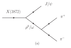
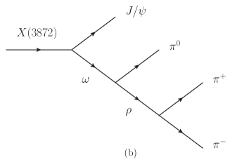
Figure 1: Feynman diagrams for the $X(3872)\to J/\psi\pi^{+}\pi^{-}$ decay with $\rho^{0}$ and $\omega$ contribution (a) and $X(3872)\to J/\psi\pi^{0}\pi^{+}\pi^{-}$ decay with $\omega$ contribution (b).

To obtain the decay amplitudes of the processes shown in Fig. 1, we need the effective interactions for these interaction vertexes, which can be described by the effective Lagrangian densities as used in Refs. Lucio-Martinez:2000now ; Xie:2008ts ; Wang:2020duv ; Janssen:1994uf :

$$\mathcal{L}_{XJ/\psi V} = g_{X}\varepsilon^{\mu\nu\rho\sigma}\partial_{\mu}X_{\nu}J/\psi_{\rho}V_{\sigma},$$ (2)

$$\mathcal{L}_{\omega\rho\pi} = g_{\omega\rho\pi}\varepsilon^{\alpha\beta\gamma\tau}\partial_{\alpha}\omega_{\gamma}\partial_{\beta}\rho_{\tau}\phi_{\pi},$$ (3)

$$\mathcal{L}_{V\pi\pi} = g_{V\pi\pi}V_{\mu}\partial^{\mu}(\phi_{\pi^{+}}-\phi_{\pi^{-}}),$$ (4)

where $X$ and $V$ represent $X(3872)$ and $\rho^{0}/\omega$ meson, respectively. While $g_{X}$, $g_{\omega\rho\pi}$, $g_{\omega\pi\pi}$, and $g_{\rho\pi\pi}$ are the coupling constants of the corresponding vertexes. In this work, we will use $g_{X_{1}}$ and $g_{X_{2}}$ for the effective coupling constants of $X(3872)$ to $J/\psi\rho^{0}$ and $J/\psi\omega$, respectively. Furthermore, we will take $g_{X}$, $g_{\omega\rho\pi}$, $g_{\rho\pi\pi}$, and $g_{\omega\pi\pi}$ as real and their values will be discussed below.

II.2 Invariant decay amplitudes

With the effective interaction Lagrangian densities given above, the invariant decay amplitudes for these diagrams shown in Fig. 1 can be written as

$$\mathcal{M}_{a} = {\cal M}_{\rho}+{\cal M}_{\omega}$$ (5)

$$= -i\left(\frac{g_{X_{1}}g_{\rho\pi\pi}}{D_{\rho}(q^{2})}F_{\rho}(q^{2})+\frac{g_{X_{2}}g_{\omega\pi\pi}}{D_{\omega}(q^{2})}F_{\omega}(q^{2})\right)\times$$

$$\varepsilon^{\mu\nu\rho\sigma}p_{\mu}\epsilon_{\nu}(p)\epsilon_{\rho}^{\ast}(p_{4})(p_{1}-p_{2})_{\sigma},$$

$$\mathcal{M}_{b} = \frac{g_{X_{2}}g_{\omega\rho\pi}g_{\rho\pi\pi}}{D_{\omega}(q^{2}_{1})D_{\rho}(q^{2}_{2})}F_{\omega}(q_{1}^{2})F_{\rho}(q_{2}^{2})\varepsilon^{\mu\nu\rho\sigma}p_{\mu}\epsilon_{\nu}(p)\epsilon_{\rho}^{\ast}(p_{4})$$ (6)

$$\times\left(-g_{\sigma\gamma}+\frac{q_{1\sigma}q_{1\gamma}}{m_{\omega}^{2}}\right)\varepsilon^{\alpha\beta\gamma\tau}q_{1\alpha}q_{2\beta}(p_{2}-p_{1})_{\tau},$$

where $p$, $p_{1}$, $p_{2}$, $p_{3}$, $p_{4}$ are the four-momenta of $X(3872)$, $\pi^{-}$, $\pi^{+}$, $\pi^{0}$, $J/\psi$, while $q_{1}$ and $q_{2}$ represent the four-momenta for the intermediate $\omega$ and $\rho^{0}$ mesons. $D_{\rho}(q^{2})$ and $D_{\omega}(q^{2}_{1})$ are the denominators of the propagators for the $\rho^{0}$ and $\omega$ meson, which are

$$D_{\rho}(q^{2}) = q^{2}-m_{\rho}^{2}+im_{\rho}\Gamma_{\rho}(q^{2}),$$ (7)

$$D_{\omega}(q^{2}_{1}) = q^{2}_{1}-m^{2}_{\omega}+im_{\omega}\Gamma_{\omega}.$$ (8)

Since the major decay channel of $\omega$ meson is the $\pi^{+}\pi^{-}\pi^{0}$ and its width is narrow, we take $m_{\omega}=782.65$ MeV and $\Gamma_{\omega}=8.49$ MeV as quoted in the Review of Particle Physics ParticleDataGroup:2020ssz . For the width of $\rho$ meson, since it is large and the predominant decay mode is $\pi\pi$, we take that $\Gamma_{\rho}$ is energy dependent, which is given by Hanhart:2010wh ; Zhang:2017eui

$$\Gamma_{\rho}(q^{2})=\Gamma_{0}\frac{|\textbf{p}_{\pi}|^{3}}{|\textbf{p}_{\pi}^{0}|^{3}}\frac{m_{\rho}^{2}}{q^{2}},$$ (9)

where

$$|\textbf{p}_{\pi}|=\frac{\sqrt{q^{2}-4m_{\pi}^{2}}}{2},~{}~{}~{}|\textbf{p}^{0}_{\pi}|=\frac{\sqrt{m_{\rho}^{2}-4m_{\pi}^{2}}}{2}.$$ (10)

In evaluating the decay amplitudes of $X(3872)\to J/\psi\pi^{+}\pi^{-}$, we include the form factors for $\rho^{0}$ and $\omega$ mesons since they are not point like particles Liu:1995st . In this work we adopt here the common scheme used in many previous works Xie:2008ts ; Xie:2014kja ; Xie:2014zga :

$$F_{\rho/\omega}(q^{2})=\frac{\Lambda_{\rho/\omega}^{4}}{\Lambda_{\rho/\omega}^{4}+(q^{2}-m_{\rho/\omega}^{2})^{2}},$$ (11)

where we assume that $\Lambda_{\rho}=\Lambda_{\omega}=\Lambda$ and they are determined to fit with the recent LHCb measurements. Note that a Blatt-Weisskopf barrier factor was used for the $P$-wave decay of a vector to $\pi\pi$ in Ref. LHCb:2022bly .

Besides, the coupling constants, $g_{\rho\pi\pi}$, $g_{\omega\pi\pi}$, and $g_{\omega\rho\pi}$, are determined from the experimentally observed partial decay widths of $\rho\to\pi\pi$, $\omega\to\pi\pi$, and $\omega\to\rho\pi\to\pi\pi\pi$, respectively. With the effective interaction Lagrangians shown in Eq. (4), these partial decay widths $\rho\to\pi\pi$ and $\omega\to\pi\pi$ can be easily calculated. The coupling constants are related to the partial decay widths as

$$\Gamma_{\rho\to\pi\pi} = \frac{g^{2}_{\rho\pi\pi}}{6\pi}\frac{p_{\rho}^{3}}{m^{2}_{\rho}},$$ (12)

$$\Gamma_{\omega\to\pi\pi} = \frac{g^{2}_{\omega\pi\pi}}{6\pi}\frac{p^{3}_{\omega}}{m^{2}_{\omega}},$$ (13)

where $p_{\rho}$ and $p_{\omega}$ are the three momenta of the $\pi$ meson in the $\rho$ or $\omega$ rest frame, respectively. With $\Gamma_{\rho\to\pi\pi}=149.1$ MeV and $\Gamma_{\omega\to\pi\pi}=0.133$ MeV as quoted in the Ref. ParticleDataGroup:2020ssz , we obtain $g_{\rho\pi\pi}=5.97$ and $g_{\omega\pi\pi}=0.18$, respectively. Note that from the partial decay width, one can only obtain the absolute value of the coupling constant, but not the phase. In this work, we assume that $g_{\rho\pi\pi}$ and $g_{\omega\pi\pi}$ are real and positive. In fact, these values obtained here were used in Refs. Janssen:1994uf ; Janssen:1996kx ; Meissner:1987ge for other processes.

In Ref. Chen:2017jcw , it was found that that $\omega$-$\rho^{0}$ mixing plays the major role in the evaluating the partial decay width of $\omega\to\pi^{+}\pi^{-}$, and its contribution is two orders of magnitude larger than that from the direct $\omega\pi\pi$ coupling. However, here we obtained the coupling constant $g_{\omega\pi\pi}$ with the experimental results of the $\omega\to\pi^{+}\pi^{-}$ decay. In other words, we have taken the effective $\omega\pi\pi$ coupling as a constant, and determined with the experimental partial decay width of $\omega\to\pi\pi$, rather than the mixing between $\rho^{0}-\omega$ with the explicit $\rho^{0}$ propagator Chen:2017jcw .

In addition, the value of $g_{\omega\rho\pi}$ is determined with the partial decay width of $\omega\to\pi^{+}\pi^{-}\pi^{0}$, which reads

$$\text{d}\Gamma_{\omega\to\pi^{+}\pi^{-}\pi^{0}}=\frac{1}{(2\pi)^{3}}\frac{1}{32m_{\omega}^{3}}|\mathcal{M}|^{2}\text{d}M_{\pi^{+}\pi^{-}}^{2}\text{d}M_{\pi^{-}\pi^{0}}^{2},$$ (14)

where

$$\mathcal{M}=\frac{-ig_{\omega\rho\pi}g_{\rho\pi\pi}}{D_{\rho}(q^{2}_{\rho})}\varepsilon_{\mu\nu\rho\sigma}q^{\mu}_{\omega}q_{\rho}\epsilon^{\nu}(q_{\omega})(p_{\pi^{+}}-p_{\pi^{-}})^{\sigma},$$ (15)

where $q_{\omega}$, $q_{\rho}$, $p_{\pi^{+}}$, and $p_{\pi^{-}}$ stand for the four-momenta of $\omega$, $\pi^{+}$, and $\pi^{-}$, respectively. With $\Gamma_{\omega\to\pi^{+}\pi^{-}\pi^{0}}=7.74$ MeV, we obtain $g_{\omega\rho\pi}=0.046$ ${\rm MeV}^{-1}$ for the case of $\Gamma_{\rho}$ energy dependent and $g_{\omega\rho\pi}=0.05$ ${\rm MeV}^{-1}$ for the case of $\Gamma_{\rho}$ as a constant. One see that the affect of the $\Gamma_{\rho}$ energy dependent is rather small and can be neglected.

II.3 Invariant mass distributions

With the formalism and ingredients given above, the calculations of the invariant mass distribution for the $X(3872)\to J/\psi\pi^{+}\pi^{-}$ and $X(3872)\to J/\psi\pi^{+}\pi^{-}\pi^{0}$ decays are straightforward ParticleDataGroup:2020ssz . The invariant $\pi^{+}\pi^{-}$ mass distribution of the $X(3872)\to J/\psi\pi^{+}\pi^{-}$ decay is given by

$$\frac{\text{d}\Gamma_{X{3872}\to J/\psi\pi^{+}\pi^{-}}}{\text{d}M_{\pi^{+}\pi^{-}}}=\frac{1}{24(2\pi)^{4}M_{X}^{2}}\times$$

$$\int\Sigma|\mathcal{M}_{2\pi}|^{2}|\mathbb{p}_{1}^{\ast}||\mathbb{p}_{4}|\text{d}\cos{\theta_{1}}\text{d}\phi_{1},$$ (16)

where $\mathbb{p}_{1}^{\ast}$ and ($\theta_{1}$, $\phi_{1}$) are the three-momentum and decay angle of the outing $\pi^{+}$ (or $\pi^{-}$) in the center-of-mass (c.m.) frame of the final $\pi^{+}\pi^{-}$ system, $\mathbb{p}_{4}$ is the three-momentum of the final $J/\psi$ meson in the rest frame of $X(3872)$, and $M_{\pi^{+}\pi^{-}}$ is the invariant mass of the final $\pi^{+}\pi^{-}$ system.

For the invariant $\pi^{+}\pi^{-}\pi^{0}$ mass distributions of the $X(3872)\to J/\psi\pi^{+}\pi^{-}\pi^{0}$ decay, it is given by,

$$\frac{\text{d}\Gamma_{X(3872)\to J/\psi\pi^{+}\pi^{-}\pi^{0}}}{\text{d}M_{\pi^{+}\pi^{-}\pi^{0}}}=\frac{1}{16(2\pi)^{7}M_{X}^{2}}\int\Sigma|\mathcal{M}_{3\pi}|^{2}\times$$

$$|\mathbb{p}_{1}^{\ast}||\mathbb{p}_{3}^{\prime}||\mathbb{p}_{4}|\text{d}M_{\pi^{+}\pi^{-}}\text{d}\cos{\theta_{1}}\text{d}\phi_{1}\text{d}\cos{\theta_{2}}\text{d}\phi_{2},$$ (17)

with $M_{\pi^{+}\pi^{-}\pi^{0}}$ the invariant mass of $\pi^{+}\pi^{-}\pi^{0}$ system. The definitions of these variables in the phase space integration are given in Appendix A.

Besides, in Eqs. (16) and (17), we take

$${\cal M}_{2\pi} = {\cal M}_{\rho}+e^{i\varphi}{\cal M}_{\omega},$$ (18)

$${\cal M}_{3\pi} = {\cal M}_{b}.$$ (19)

Note that we have included a free parameter $\varphi$ which stands for the relative phase between $\omega$ and $\rho^{0}$ terms for the $X(3872)\to J/\psi\pi^{+}\pi^{-}$ decay. On the other hand, more details for the integration of the multi-body phase space can be found in Refs. Xie:2015zga ; Xie:2018gbi ; Jing:2020tth .

III Numerical results and discussions

In this section, we present the numerical results for the invariant mass distribution of $\pi^{+}\pi^{-}$ of the $X(3872)\to J/\psi\pi^{+}\pi^{-}$ decay. To compare the theoretical invariant mass distributions with the experimental measurements, we introduce an extra global normalization factor $C$, which will be fitted to the experimental data. In the calculation, the masses, widths and spin-parities of the involved particles are listed in Table 1.

Table 1: Masses, widths and spin-parities of the involved particles in this work.

Particle	Mass (MeV)	Width (MeV)	Spin-parity ($J^{P}$)
$X(3872)$	3871.69	1.19$\pm$0.21	$1^{+}$
$J/\psi$	3096.9	—	$1^{-}$
$\rho^{0}$	775.26	149.1$\pm$0.8	$1^{-}$
$\omega$	782.66	8.68$\pm$0.13	$1^{-}$
$\pi^{+}/\pi^{-}$	139.57	—	$0^{-}$
$\pi^{0}$	134.97	—	$0^{-}$

We perform four parameters ($R_{X}\equiv g_{X_{1}}/g_{X_{2}}$, $Cg_{X_{2}}^{2}$, $\Lambda$, and $\varphi$) $\chi^{2}$ fits to the experimental data on the $\pi^{+}\pi^{-}$ invariant mass distributions. We will study two types of fit: one takes the total width of $\rho$ energy dependent, while the other one takes the total width of $\rho$ as a constant. The fitted parameters and the corresponding $\chi^{2}/\mathrm{d.o.f.}$ are shown in Table 2. We have checked that the results of the two fits are very similar, this indicates that the affects of the energy dependent of the $\rho$ total width $\Gamma_{\rho}$ is very small and can be neglected. It is worth to mention that the obtained ratio $R_{X}$ is very similar with these values $0.29\pm 0.04$ and $0.26^{+0.08}_{-0.05}$ obtained in Ref. LHCb:2022bly and Ref. Hanhart:2011tn , respectively.

Although the two parameters $R_{X}$ and $Cg_{X_{2}}^{2}$ can be obtained from the fit directly, the physical couplings $g_{X_{1}}$ and $g_{X_{2}}$ can only be extracted with the further inputs. With the value $R_{X}=0.25\pm 0.01$, the coupling $g_{X_{2}}=0.33\pm 0.06$ can be extracted from the the branching ratio $\mathcal{B}(X(3872)\to J/\psi\pi^{+}\pi^{-})=(3.8\pm 1.2)\%$ ParticleDataGroup:2020ssz . Consequently, the coupling $g_{X_{1}}=0.08\pm 0.02$ and the normalization factor $C=(7.48\pm 2.78)\times 10^{-5}$ can be obtained. The above values have been listed in Table 2 as well as those for the constant $\Gamma_{\rho}$ case.

Table 2: The fitted and determined parameters in this work. The second and third columns are the fitted results of the $\Gamma_{\rho}(q^{2})$ energy-dependent fit and fixed $\Gamma_{0}$ fit, respectively.

Number	1	2
$\rho$ meson width	$\Gamma_{\rho}(q^{2})$ energy dependent	$\Gamma_{0}$ constant
$R_{X}$	$0.25\pm 0.01$	$0.30\pm 0.01$
$Cg_{X_{2}}^{2}~{}(\times 10^{4})$	$8.31\pm 0.45$	$7.10\pm 0.48$
$\Lambda$ (MeV)	$612\pm 18$	$598\pm 16$
$\varphi~{}(\degree)$	$128.9\pm 8.0$	$134.5\pm 7.7$
$\chi^{2}/\mathrm{d.o.f.}$	$0.6$	$0.6$
$g_{X_{1}}$	$0.08\pm 0.02$	$0.09\pm 0.02$
$g_{X_{2}}$	$0.33\pm 0.06$	$0.31\pm 0.06$
$C~{}(\times 10^{5})$	$7.48\pm 2.78$	$7.48\pm 2.81$

With the central values of Table 2 for the case of $\Gamma_{\rho}$ energy dependent, the $\pi^{+}\pi^{-}$ invariant mass distribution is shown by the red curve in Fig. 2. Note that the results for the case of $\Gamma_{\rho}$ as a constant are very similar with the ones obtained for the case of $\Gamma_{\rho}$ energy dependent. In Fig. 2, the red-solid curve stands for the total contributions from the $\rho^{0}$ and $\omega$ mesons, the blue-dash-dotted and green-dash-dotted curves correspond to the contribution from only the $\rho^{0}$ and $\omega$, respectively, while the black-dash-dotted stands for their interference. The band accounts for the corresponding $68\%$ confidence-level interval deduced from the distributions of the fitted parameters shown in Table 2. One can see that the total numerical results can explain the experimental data quite well. Furthermore, the contribution of $\rho$ meson is predominant in the whole energy region consider for the $M_{\pi^{+}\pi^{-}}$, while the contribution of $\omega$ meson is crucial to the $\pi^{+}\pi^{-}$ invariant mass distributions at high energy of $M_{\pi^{+}\pi^{-}}$.

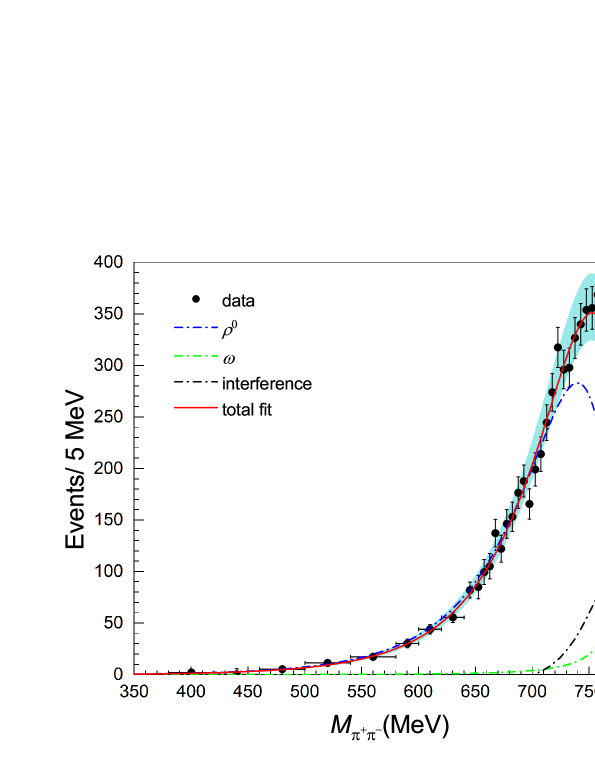
Figure 2: Invariant mass distribution of $\pi^{+}\pi^{-}$ for the $X(3872)\to J/\psi\pi^{+}\pi^{-}$ decay, compared with the experimental data taken from Ref. LHCb:2022bly . The blue-dash-dotted, green-dash-dotted curves and black-dash-dotted are the contributions from the $\rho^{0}$, $\omega$, and their interference, respectively. The red solid one is their total contribution. The band accounts for the corresponding $68\%$ confidence-level interval deduced from the distributions of the fitted parameters shown in Table 2

With the fitted couplings $g_{X_{1}}$ and $g_{X_{2}}$, one can easily obtain the $\omega$ contribution, without the $\rho^{0}$-$\omega$ interference terms, to the total $X(3872)\to J/\psi\pi^{+}\pi^{-}$ decay as

$$\frac{\Gamma_{X(3872)\to J/\psi\omega\to J/\psi\pi^{+}\pi^{-}}}{\Gamma_{X(3872)\to J/\psi\pi^{+}\pi^{-}}}=(4.7\pm 2.4)\%$$ (20)

for the case of $\Gamma_{\rho}$ energy dependent and

$$\frac{\Gamma_{X(3872)\to J/\psi\omega\to J/\psi\pi^{+}\pi^{-}}}{\Gamma_{X(3872)\to J/\psi\pi^{+}\pi^{-}}}=(4.0\pm 2.1)\%$$ (21)

for the case of $\Gamma_{\rho}$ as a constant. These values agree with the value $(1.9\pm 0.4\pm 0.3)\%$, obtained by the LHCb analysis in Ref. LHCb:2022bly within one standard deviation.

It is customary to apply the so-called narrow width approximation in the case where a particle decays into two particles and one of them with narrow width subsequently decays into other two particles in the final state Cheng:2020iwk ; Cheng:2020mna . Since the width of $\omega$ meson is so narrow, we can extract the branching fraction of the quasi-two-body decay $X(3872)\to J/\psi\omega$

$${\cal B}(X(3872)\to J/\psi\omega)$$ (22)

$$= \frac{{\cal B}(X(3872)\to J/\psi\omega\to J/\psi\pi^{+}\pi^{-})}{{\cal B}(\omega\to\pi^{+}\pi^{-})}$$

$$= (11.5\pm 7.5)\%,$$

within the narrow width approximation. Furthermore, we extract the branching ratio fraction between the $J/\psi\omega$ and $J/\psi\pi^{+}\pi^{-}$ modes as defined in Ref. BESIII:2019qvy .

$$\mathcal{R}\equiv\frac{{\cal B}(X(3872)\to J/\psi\omega)}{{\cal B}(X(3872)\to J/\psi\pi^{+}\pi^{-})}=3.0\pm 2.2$$ (23)

for the $\Gamma_{\rho}$ energy-dependent case, and

$${\cal B}(X(3872)\to J/\psi\omega)=(9.9\pm 6.3)\%,$$ (24)

$$\mathcal{R}=2.6\pm 1.9$$ (25)

for the constant $\Gamma_{\rho}$ case. The two values of $\mathcal{R}$ are in agreement with the experimental measurements $1.6^{+0.4}_{-0.3}\pm 0.2$ by BESIII collaboration BESIII:2019qvy within uncertainties.

Next we turn to the $X(3872)\to J/\psi\pi^{+}\pi^{-}\pi^{0}$ decay. With the values of $g_{X_{1}}$ and $g_{X_{2}}$, we obtain:

$${\cal B}[X(3872)\to J/\psi\pi^{+}\pi^{-}\pi^{0}]=(1.1\pm 0.5)\%,$$ (26)

for the $\Gamma_{\rho}$ energy-dependent case and

$${\cal B}[X(3872)\to J/\psi\pi^{+}\pi^{-}\pi^{0}]=(1.4\pm 0.6)\%,$$ (27)

for the constant $\Gamma_{\rho}$ case. Those values are in agreement with both the experimental measurements ParticleDataGroup:2020ssz and the theoretical calculations in Ref. Aceti:2012cb .

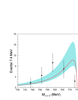
Figure 3: Invariant mass distribution of $\pi^{+}\pi^{-}\pi^{0}$ for the $X(3872)\to J/\psi\pi^{+}\pi^{-}\pi^{0}$ decay, compared with the experimental data taken from Ref. BaBar:2010wfc .

Finally, with these model parameters determined by fitting to the $\pi^{+}\pi^{-}$ invariant mass distributions for the $X(3872)\to J/\psi\pi^{+}\pi^{-}$ decay, we calculate the $\pi^{+}\pi^{-}\pi^{0}$ invariant mass distributions for the $X(3872)\to J/\psi\pi^{+}\pi^{-}\pi^{0}$ decay. The numerical results are shown as the red curve in Fig. 3. The error band of the theoretical calculations are obtained from the uncertainty of the parameter $g_{X_{2}}$ which stems from the uncertainties of both the two pion invariant mass distribution of the $J/\psi\pi^{+}\pi^{-}$ decay mode, i.e. the fitted parameter $R_{X}$, and the $X(3872)\to J/\psi\pi^{+}\pi^{-}$ branching ratio. To compare the theoretical invariant mass distributions with the experimental measurements, we have to introduce again an extra global normalization factor $C_{3\pi}$. In Fig. 3 the red-solid curve has been adjusted to the strength of the inverse-second data point of BABAR BaBar:2010wfc by taking $C_{3\pi}=6.07\times 10^{4}$ for the $\Gamma_{\rho}$ energy-dependent case. For the constant $\Gamma_{\rho}$ case, the value of $C_{3\pi}$ is $5.77\times 10^{4}$, and the line shape of the $\pi^{+}\pi^{-}\pi^{0}$ invariant mass distributions is almost the same. As shown in Fig. 3, most of the experimental data locate in the theoretical one sigma region. This can be tested by future precise measurements for the $X(3872)\to J/\psi\pi^{+}\pi^{-}\pi^{0}$ channel. In addition, further more precise measurements of the $X(3872)\to J/\psi\pi^{+}\pi^{-}$ channel can also help to reduce the uncertainty of the couplings $g_{X_{1}}$ and $g_{X_{2}}$. The $g_{X_{2}}$ can also constrain the data in $J/\psi\pi^{+}\pi^{-}\pi^{0}$ channel.

IV Summary

In summary, we have performed a theoretical calculation for the processes of $X(3872)\to J/\psi\pi^{+}\pi^{-}$ and $J/\psi\pi^{+}\pi^{-}\pi^{0}$. For the $X(3872)\to J/\psi\pi^{+}\pi^{-}$ decay, in addition to the dominant contribution from the $\rho^{0}$ meson, the contribution of the intermediate $\omega$ meson with an effective $\omega\pi\pi$ coupling is also considered in our framework. It is found that the recent LHCb experimental measurements on the $\pi^{+}\pi^{-}$ invariant mass distributions LHCb:2022bly can be well reproduced. Meanwhile, the ratio of the couplings between $X(3872)\to J/\psi\rho^{0}$ and $X(3872)\to J/\psi\omega$ is determined, which is consistent with the previous analysis in Refs. Hanhart:2011tn ; LHCb:2022bly .

Furthermore, with the model parameters determined from the $\pi^{+}\pi^{-}$ invariant mass distribution of the $X(3872)\to J/\psi\pi^{+}\pi^{-}$ decay, the $X(3872)\to J/\psi\pi^{+}\pi^{-}\pi^{0}$ branching fraction and the corresponding $\pi^{+}\pi^{-}\pi^{0}$ invariant mass distributions are extracted, which are also in agreement with the available experimental data with large errors. This kind of results could be tested by the future precise measurements.

Appendix A Four-body phase space

In this appendix, we provide the definitions of those variables in the phase space integration of Eq. (17), which are explicitly shown in Fig. 4. The $\mathbb{p}_{1}^{\ast}$ and ($\theta_{1}$, $\phi_{1}$) are the three-momentum and decay angles of the outing $\pi^{-}$ in the $\pi^{+}\pi^{-}$ center-of-mass (c.m.) frame. The $\mathbb{p}^{\prime}_{3}$ and ($\theta_{2}$, $\phi_{2}$) are the three-momentum and decay angles of the outing $\pi^{0}$ in the $\pi^{+}\pi^{-}\pi^{0}$ c.m. frame. The $\mathbb{p}_{4}$ is the three-momentum of the final $J/\psi$ meson in the $X(3872)$ rest frame.

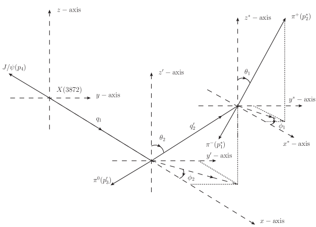
Figure 4: The definitions of these variables in the phase space integration of the $X(3872)\to J/\psi\omega\to J/\psi\pi^{+}\pi^{-}\pi^{0}$ decay.

References

- (1) S. K. Choi et al. [Belle], Phys. Rev. Lett. 91, 262001 (2003) [arXiv:hep-ex/0309032 [hep-ex]].
- (2) S. K. Choi et al. [Belle], Phys. Rev. D 84, 052004 (2011) [arXiv:1107.0163 [hep-ex]].
- (3) R. Aaij et al. [LHCb], Phys. Rev. Lett. 110, 222001 (2013) [arXiv:1302.6269 [hep-ex]].
- (4) P. A. Zyla et al. [Particle Data Group], PTEP 2020, no.8, 083C01 (2020)
- (5) S. Godfrey and N. Isgur, Phys. Rev. D 32, 189-231 (1985)
- (6) R. Aaij et al. [LHCb], Phys. Rev. D 102, no.9, 092005 (2020) [arXiv:2005.13419 [hep-ex]].
- (7) R. Aaij et al. [LHCb], JHEP 08, 123 (2020) [arXiv:2005.13422 [hep-ex]].
- (8) R. F. Lebed, R. E. Mitchell and E. S. Swanson, Prog. Part. Nucl. Phys. 93, 143-194 (2017) [arXiv:1610.04528 [hep-ph]].
- (9) H. X. Chen, W. Chen, X. Liu and S. L. Zhu, Phys. Rept. 639, 1-121 (2016) [arXiv:1601.02092 [hep-ph]].
- (10) A. Esposito, A. Pilloni and A. D. Polosa, Phys. Rept. 668, 1-97 (2017) [arXiv:1611.07920 [hep-ph]].
- (11) S. L. Olsen, T. Skwarnicki and D. Zieminska, Rev. Mod. Phys. 90, no.1, 015003 (2018) [arXiv:1708.04012 [hep-ph]].
- (12) F. K. Guo, C. Hanhart, U.-G. Meißner, Q. Wang, Q. Zhao and B. S. Zou, Rev. Mod. Phys. 90, no.1, 015004 (2018) [erratum: Rev. Mod. Phys. 94, no.2, 029901 (2022)] [arXiv:1705.00141 [hep-ph]].
- (13) A. Ali, J. S. Lange and S. Stone, Prog. Part. Nucl. Phys. 97, 123-198 (2017) [arXiv:1706.00610 [hep-ph]].
- (14) N. Brambilla, S. Eidelman, C. Hanhart, A. Nefediev, C. P. Shen, C. E. Thomas, A. Vairo and C. Z. Yuan, Phys. Rept. 873, 1-154 (2020) [arXiv:1907.07583 [hep-ex]].
- (15) Y. R. Liu, H. X. Chen, W. Chen, X. Liu and S. L. Zhu, Prog. Part. Nucl. Phys. 107, 237-320 (2019) [arXiv:1903.11976 [hep-ph]].
- (16) F. K. Guo, X. H. Liu and S. Sakai, Prog. Part. Nucl. Phys. 112, 103757 (2020) [arXiv:1912.07030 [hep-ph]].
- (17) X. K. Dong, F. K. Guo and B. S. Zou, Commun. Theor. Phys. 73, no.12, 125201 (2021) [arXiv:2108.02673 [hep-ph]].
- (18) H. X. Chen, W. Chen, X. Liu, Y. R. Liu and S. L. Zhu, [arXiv:2204.02649 [hep-ph]].
- (19) F. K. Guo, Phys. Rev. Lett. 122, no.20, 202002 (2019) [arXiv:1902.11221 [hep-ph]].
- (20) Z. H. Zhang and F. K. Guo, Phys. Rev. Lett. 127, no.1, 012002 (2021) [arXiv:2012.08281 [hep-ph]].
- (21) D. Gamermann and E. Oset, Phys. Rev. D 80, 014003 (2009) [arXiv:0905.0402 [hep-ph]].
- (22) N. Li and S. L. Zhu, Phys. Rev. D 86, 074022 (2012) [arXiv:1207.3954 [hep-ph]].
- (23) L. Meng, G. J. Wang, B. Wang and S. L. Zhu, Phys. Rev. D 104, no.9, 094003 (2021) [arXiv:2109.01333 [hep-ph]].
- (24) N. A. Tornqvist, Phys. Lett. B 590, 209-215 (2004) [arXiv:hep-ph/0402237 [hep-ph]].
- (25) S. Takeuchi, K. Shimizu and M. Takizawa, Few Body Syst. 54, 419-423 (2013) [arXiv:1110.3694 [hep-ph]].
- (26) K. Terasaki, Prog. Theor. Phys. 122, 1285-1290 (2010) [arXiv:0904.3368 [hep-ph]].
- (27) S. Takeuchi, K. Shimizu and M. Takizawa, PTEP 2014, no.12, 123D01 (2014) [erratum: PTEP 2015, no.7, 079203 (2015)] [arXiv:1408.0973 [hep-ph]].
- (28) [LHCb], [arXiv:2204.12597 [hep-ex]].
- (29) A. Abulencia et al. [CDF], Phys. Rev. Lett. 96, 102002 (2006) [arXiv:hep-ex/0512074 [hep-ex]].
- (30) M. Ablikim et al. [BESIII], Phys. Rev. Lett. 122, no.23, 232002 (2019) [arXiv:1903.04695 [hep-ex]].
- (31) K. Abe et al. [Belle], [arXiv:hep-ex/0505037 [hep-ex]].
- (32) P. del Amo Sanchez et al. [BaBar], Phys. Rev. D 82, 011101 (2010) [arXiv:1005.5190 [hep-ex]].
- (33) C. Hanhart, Y. S. Kalashnikova, A. E. Kudryavtsev and A. V. Nefediev, Phys. Rev. D 85, 011501 (2012) [arXiv:1111.6241 [hep-ph]].
- (34) M. Suzuki, Phys. Rev. D 72, 114013 (2005) [arXiv:hep-ph/0508258 [hep-ph]].
- (35) X. Liu, B. Zhang and S. L. Zhu, Phys. Lett. B 645, 185-188 (2007) [arXiv:hep-ph/0610278 [hep-ph]].
- (36) D. Gamermann, J. Nieves, E. Oset and E. Ruiz Arriola, Phys. Rev. D 81, 014029 (2010) [arXiv:0911.4407 [hep-ph]].
- (37) S. Coito, G. Rupp and E. van Beveren, Eur. Phys. J. C 71, 1762 (2011) [arXiv:1008.5100 [hep-ph]].
- (38) M. Albaladejo, F. K. Guo, C. Hidalgo-Duque, J. Nieves and M. P. Valderrama, Eur. Phys. J. C 75, no.11, 547 (2015) [arXiv:1504.00861 [hep-ph]].
- (39) Q. Wu, D. Y. Chen and T. Matsuki, Eur. Phys. J. C 81, no.2, 193 (2021) [arXiv:2102.08637 [hep-ph]].
- (40) J. L. Lucio-Martinez, M. Napsuciale, M. D. Scadron and V. M. Villanueva, Phys. Rev. D 61, 034013 (2000)
- (41) J. J. Xie, C. Wilkin and B. S. Zou, Phys. Rev. C 77, 058202 (2008) [arXiv:0802.2802 [nucl-th]].
- (42) Y. Wang, Q. Wu, G. Li, J. J. Xie and C. S. An, Eur. Phys. J. C 80, no.5, 475 (2020) [arXiv:2005.04665 [hep-ph]].
- (43) G. Janssen, K. Holinde and J. Speth, Phys. Rev. C 49, 2763-2776 (1994)
- (44) C. Hanhart, Y. S. Kalashnikova and A. V. Nefediev, Phys. Rev. D 81, 094028 (2010) [arXiv:1002.4097 [hep-ph]].
- (45) X. Zhang and J. J. Xie, Commun. Theor. Phys. 70, no.1, 060 (2018) [arXiv:1712.05572 [nucl-th]].
- (46) L. C. Liu, Q. Haider and J. T. Londergan, Phys. Rev. C 51, 3427-3434 (1995) [arXiv:nucl-th/9503009 [nucl-th]].
- (47) J. J. Xie, E. Wang and B. S. Zou, Phys. Rev. C 90, no.2, 025207 (2014) [arXiv:1405.5586 [nucl-th]].
- (48) J. J. Xie, J. J. Wu and B. S. Zou, Phys. Rev. C 90, no.5, 055204 (2014) [arXiv:1407.7984 [nucl-th]].
- (49) G. Janssen, K. Holinde and J. Speth, Phys. Rev. C 54, 2218-2234 (1996)
- (50) U.-G. Meissner, Phys. Rept. 161, 213 (1988)
- (51) Y. H. Chen, D. L. Yao and H. Q. Zheng, Commun. Theor. Phys. 69, no.1, 50 (2018) [arXiv:1710.11448 [hep-ph]].
- (52) J. J. Xie, Y. B. Dong and X. Cao, Phys. Rev. D 92, no.3, 034029 (2015) [arXiv:1506.01133 [hep-ph]].
- (53) J. J. Xie and E. Oset, Phys. Lett. B 792, 450-453 (2019) [arXiv:1811.07247 [hep-ph]].
- (54) H. J. Jing, C. W. Shen and F. K. Guo, Science Bulletin 66, no.7, 653-656 (2021) [arXiv:2005.01942 [hep-ph]].
- (55) H. Y. Cheng, C. W. Chiang and C. K. Chua, Phys. Rev. D 103, no.3, 036017 (2021) [arXiv:2011.07468 [hep-ph]].
- (56) H. Y. Cheng, C. W. Chiang and C. K. Chua, Phys. Lett. B 813, 136058 (2021) [arXiv:2011.03201 [hep-ph]].
- (57) F. Aceti, R. Molina and E. Oset, Phys. Rev. D 86, 113007 (2012) [arXiv:1207.2832 [hep-ph]].