Hypothesis Testing for Differentially Private Linear Regression

Abstract

In this work, we design differentially private hypothesis tests for the following problems in the general linear model: testing a linear relationship and testing for the presence of mixtures. The majority of our hypothesis tests are based on differentially private versions of the $F$-statistic for the general linear model framework, which are uniformly most powerful unbiased in the non-private setting. We also present other tests for these problems, one of which is based on the differentially private nonparametric tests of Couch, Kazan, Shi, Bray, and Groce (CCS 2019), which is especially suited for the small dataset regime. We show that the differentially private $F$-statistic converges to the asymptotic distribution of its non-private counterpart. As a corollary, the statistical power of the differentially private $F$-statistic converges to the statistical power of the non-private $F$-statistic. Through a suite of Monte Carlo based experiments, we show that our tests achieve desired significance levels and have a high power that approaches the power of the non-private tests as we increase sample sizes or the privacy-loss parameter. We also show when our tests outperform existing methods in the literature.

1 Introduction

Linear regression is one of the most fundamental statistical techniques available to social scientists and economists (especially econometricians). One of the goals of performing regression analysis is for use in decision-making via point estimation (i.e., getting a single predicted value for the dependent variable). To increase the confidence of decision-makers and analysts in such estimates, it is often important to also release accompanying uncertainty estimates for the point estimates [14, 15, 17, 4].

In this work, we aim to provide differentially private linear regression uncertainty quantification via the use of hypothesis tests. Given the realistic possibility of reconstruction, membership, and inference attacks [45, 25], we can rely on Differential Privacy (DP), a rigorous approach to quantifying privacy loss [24, 22]. The task of DP linear regression is to, given datapoints $\{(x_{i},y_{i})\}_{i=1}^{n}$, estimate point or uncertainty estimates for linear regression while satisfying differential privacy. The majority of our tests will rely on generalized likelihood ratio test $F$-statistics.

In previous works [42, 48, 21, 6], differentially private estimators for linear regression are explored and key factors (such as sample size and variance of the independent variable) that affect the accuracy of these estimators are identified. The focus of these previous works is for point estimate prediction. The predictive accuracy of such estimators can be measured in terms of a confidence bound or mean-squared error. We continue the study of the utility of such estimators for use in uncertainty quantification via hypothesis testing [42]. (See Section 2 for background on hypothesis testing.)

Earlier work on uncertainty quantification for linear regression was done by Sheffet [42], who constructed confidence intervals and hypothesis tests based on the $t$-test statistic, and can be used to test a linear relationship. The random projection routine in [42], based on the Johnson–Lindenstrauss (JL) transform, only starts to correctly reject the null hypothesis when the sample size is very large (or the variables have a large spread). This observation is also supported by the work of [19]. Furthermore, the random projection routine requires extra parameters (e.g., for specifying the dimensions of the random matrix). In our work, we use the $F$-statistic and our framework can be used to test mixture models, amongst other tests. We provide a general framework for DP tests based on the $F$-statistic. In addition, we will consider hypothesis testing for linear regression coefficients on both small and large datasets. For the mixture model tester, we additionally adapt and evaluate a nonparametric method, a DP analogue of the Kruskal-Wallis test due to Couch, Kazan, Shi, Bray, and Groce [19], which is especially suited for the small dataset regime. To the best of our knowledge, our tests are the first to differentially privately detect mixtures in linear regression models, with accompanying experimental validation.

1.1 Our Contributions

In this work, we show that for the problem of differentially private linear regression, we can perform hypothesis testing for two problems in the general linear model:

1. Testing a Linear Relationship: is the slope of the linear model equal to some constant (e.g., slope is 0)?

2. Testing for Mixtures: does the population consist of one or more sub-populations with different regression coefficients?

We provide a differentially private analogue of the $F$-statistic which we, under the general linear model, show converges in distribution to the asymptotic distribution of the $F$-statistic (Theorem 5.1). Furthermore, the DP regression coefficients converge, in probability, to the true coefficients (Lemma 5.11). In particular, in Lemma 5.11, we show a $1/\sqrt{n}$ statistical rate of convergence for the DP regression coefficients used for our hypothesis tests. This matches the optimal rate [38]. We then use our DP $F$-statistic and parametric estimates to obtain DP hypothesis tests using a Monte Carlo parametric bootstrap, following Gaboardi, Lim, Rogers, and Vadhan [30]. The Monte Carlo parametric bootstrap is used to ensure that our tests achieve a target significance level of $\alpha$ (i.e., data generated under the null hypothesis is rejected with probability $\alpha$). We experimentally compare these tests to their non-private counterparts for univariate linear regression (i.e., one independent variable and one dependent variable). To the best of our knowledge, our tests are the first that use the $F$-statistic to perform tests on the problem of linear regression while ensuring privacy of the data subjects. In addition, our $F$-statistic based tests can be adapted to work on design matrices in any dimension. i.e., the design matrix can be cast in the form $X\in{\mathbb{R}}^{n\times p}$ for any integer $p\geq 2$ where $n$ represents the number of individuals in the dataset and $p$ represents the number of features per individual; we leave experimental evaluation of the multivariate case for future work.

Experimental evaluation of our hypothesis tests is done on:

1. Synthetic Data: We generate synthetic datasets with different distributions on the independent (or explanatory) variables. Specifically, we consider uniform, normal, and exponential distributions on the independent variables. We also vary the noise distribution of the dependent variable.

2. Opportunity Insights (OI) Data: We use a simulated version of the data used by the Opportunity Insights team (an economics research lab) to release the Opportunity Atlas tool, primarily used to predict social and economic mobility. We chose to use these datasets since they come from a real deployment of privacy-preserving statistics. The census tract-level datasets from these states can have a very small number of datapoints.

3. Bike Sharing Dataset: We use a real-world dataset publicly available in the UCI machine learning repository. The dataset consists of daily and hourly counts (with other information such as seasonal and weather information) of bike rentals in the Capital bikeshare system in years 2011 and 2012.

Our experimental findings are as follows:

1. Significance: Across a variety of experimental settings, the significance is below the target significance level of 0.05. Thus, we have a high confidence that we will not falsely reject the null hypothesis, should the null hypothesis be true. Our tests are designed to be conservative in the sense that they err on the side of failing to reject the null (e.g., when the DP estimate of a variance is negative).

2. Power: Consistently, the power of our tests increase as we increase sample sizes (from hundreds up to tens of thousands) or as we relax the privacy parameter. The behavior of our DP tests tends toward that of the non-DP tests. The power of the DP OLS linear relationship tester increases as the slope of the model increases and as the noise in the dependent variable decreases. But when the DP estimate of the noise in the dependent variable is negative, the tests err on the side of failing to reject the null, leading to a lower power. The power of the mixture model tests also increases as the difference between the slopes in the two groups increases. And the more uneven the group sizes are, the lower the power.

3. Alternative Method 1: We compare our DP linear relationship tester, based on the $F$-statistic, to a test that builds on a DP parametric bootstrap method for confidence interval estimation due to Ferrando, Wang, and Sheldon [29]. They prove that these intervals are consistent (in the asymptotic regime) and experimentally show that these intervals have good coverage. We can rely on such confidence intervals to decide to reject or fail to reject the null hypothesis. Such methods achieve the desired significance levels. However, we observe that the method is less powerful than the $F$-statistic approach. This behavior could be attributed to the differences in the bootstrap process: whereas we use estimates of sufficient statistics under the null in the bootstrap procedure, Ferrando et al. [29] uses the entirety of the sufficient statistics estimated for the parametric model.

4. Alternative Method 2: Inspired by the DP regression estimators of  [23, 6], we also show how to reduce linear relationship testing to the problem of testing if data is generated from a Bernoulli distribution with equal chance of outputting heads or tails. This problem has simple DP tests and has been solved optimally by Awan and Slavkovic [7] for pure DP (whereas we use zCDP). The resulting linear relationship tester is nonparametric in that, in contrast to the $F$-statistic, it does not assume that the residuals are normally distributed. We find that this nonparametric test outperforms our DP $F$-statistic on smaller privacy-loss parameters or larger slopes, but otherwise the $F$-statistic performs better.

5. Alternative Method 3: For testing mixture models, we also give a reduction to testing whether two groups have the same median, which can be solved using the DP nonparametric method of Couch, Kazan, Shi, Bray, and Groce [19]. We find that this nonparametric test has a higher power in the small dataset regime than the DP $F$-statistic method. As the dataset size increases or the difference in slopes between the groups increases, the gap closes. In addition, as the variance of the independent variable increases, the $F$-statistic method outperforms the nonparametric method.

1.2 Overview of Techniques

We provide Algorithm 1, a generic framework for DP Monte Carlo tests via a parametric bootstrap routine for estimating sufficient statistics. Algorithm 1 crucially relies on DPStats, a procedure that uses statistics of the independent and dependent variables to produce DP statistics. These statistics can be used to decide to reject or fail to reject the null hypothesis. DPStats must satisfy DP—in our case $\rho$-zCDP (Zero-Concentrated Differential Privacy). Algorithms 2 and 4 are SSP (Sufficient Statistic Perturbation) implementations of DPSS for the linear relationship tester and mixture model tester, respectively. (See Section 4.2 for more details.) Algorithm 5 is a DP nonparametric test framework based on the Kruskal-Wallis test statistic for testing mixtures. We use the standard Gaussian mechanism to make these algorithms satisfy zCDP although the Laplace mechanism could be used instead (i.e., for pure DP). To make Algorithm 5 DP, we randomly pair datapoints so that the resulting transformation is 1-Lipschitz. i.e., changing one datapoint will change a single slope estimate. See Section 4.3 for more details.

Theorem 5.1 shows that the DP $F$-statistic converges to the asymptotic distribution of its non-private counterpart, the chi-squared distribution. As a corollary, the statistical power of the DP $F$-statistic converges to the statistical power of the non-private $F$-statistic. To prove this result, we first show the $1/\sqrt{n}$ statistical rate of convergence for the DP coefficients. Then we reformulate both the $F$-statistic and the DP $F$-statistic in terms of the $1/\sqrt{n}$ convergent quantities, including convergent functions of the Gram Matrix of the independent variable. Next, we construct random variables whose $\ell_{2}$-norm squared is distributed as the (non-central) chi-squared distribution. Then we prove that DP analogues of the squared $\ell_{2}$-norm of such random variables converge to the (non-central) chi-squared distribution. Finally, using such random variables, the reformulated DP $F$-statistic, reformulated $F$-statistic, and the continuous mapping theorem, we combine the convergent quantities to prove Theorem 5.1. See Section 5 for more details.

1.3 Other Related Work

Differentially Private Linear Regression

Sheffet [42] considers hypothesis testing for ordinary least squares for a specific test: testing for a linear relationship under the assumption that the independent variable is drawn from a normal distribution. Wang  [48] focuses on using adaptive algorithms for linear regression prediction.

$M$-estimators [33], motivated by the field of robust statistics [35], are a simple class of statistical estimators that present a general approach to parametric inference. Dwork and Lei [23, 38] and Chaudhuri and Hsu [16] present differentially private $M$-estimators with near-optimal statistical rates of convergence. Avella-Medina [5] generalizes the $M$-estimator approach to differentially private statistical inference using an empirical notion of influence functions to calibrate the Gaussian mechanism. Alabi, McMillan, Sarathy, Smith, and Vadhan [6] proposed median-based estimators for linear regression and evaluated their performance for prediction. All of these previous works show connections between robust statistics, $M$-estimators, and differential privacy. The ordinary least squares estimator is a classical $M$-estimator for prediction. Other examples include sample quantiles and the maximum likelihood estimation (MLE) objective. However, for differentially private hypothesis testing, as we show in this work, the optimal test statistic for DP linear regression depends on statistical properties of the dataset (such as variance and sample size). We also present novel differentially private test statistics that converge in distribution to the asymptotic distribution of the $F$-statistic.

Bernstein and Sheldon [12] take a Bayesian approach to linear regression prediction and credible interval estimation. Through the Bayesian lens, there is also work on how to approximately bias-correct some DP estimators while providing some uncertainty estimates in terms of (private) standard errors [27]. As a motivation for differentially private simple linear regression point and uncertainty estimation, Bleninger, Dreschsler, Ronning [9] show how an attacker could use background information to reveal sensitive attributes about data subjects used in a simple linear regression analysis.

General Differentially Private Hypothesis Testing

Gaboardi, Lim, Rogers, and Vadhan  [30] study hypothesis testing subject to differential privacy constraints. The tests they consider are: (1) goodness-of-fit tests on multinomial data to determine if data was drawn from a multinomial distribution with a certain probability vector, and (2) independence tests for checking whether two categorical random variables are independent of each other. Both tests use the chi-squared test statistic. Rogers and Kifer  [40] develop new test statistics for differentially private hypothesis testing on categorical data while maintaining a given Type I error. Through the use of the subsample-and-aggregate framework, Barrientos et al. [10] compute univariate $t$-statistics by first partitioning the data into $M$ disjoint subsets, estimating the statistic on each subset, truncating the statistic at some threshold $a$, and then adding noise from a Laplace distribution to the average of the truncated $t$-statistics. Our framework requires a clipping parameter (similar to $a$) but does not require any others (e.g., the number of subsets). As noted in that work, the parameter $M$ plays a significant role in the performance—and tuning—of their tests while our tests require no such parameter tuning on partitioning of the data.

A subset of previous work [46, 13, 41, 19] focus on differentially private independence tests between a categorical and continuous variables. Some of these works produce nonparametric tests which require little or no distributional assumptions on the data generation process. Specifically, Couch, Kazan, Shi, Bray, and Groce [19] develop DP analogues of rank-based nonparametric tests such as Kruskal-Wallis and Mann-Whitney signed-rank tests. The Kruskal-Wallis test, for example, can be used to determine whether the medians of two or more groups are the same. We adapt their test to the setting of linear regression by using it to compare the distributions of slopes between the two groups. Wang, Lee, and Kifer [49] develop DP versions of likelihood ratio and chi-squared tests, showing a modified equivalence between chi-squared and likelihood ratio tests.

In the space of differentially private hypothesis testing, previous work introduce methods for differentially private identity and equivalence testing of discrete distributions [1, 8, 2, 3]. A differentially private version of the log-likelihood ratio test for the Neyman-Pearson lemma has also been shown to exist [18]. Furthermore, Awan and Slavkovic [7] derive uniformly most powerful DP tests for simple hypotheses for binomial data. Suresh [44] proposes a hypothesis test, which can be made to satisfy differential privacy, that is robust to distribution perturbations under Hellinger distance. Sheffet and Kairouz, Oh, Viswanath  [43, 37] also consider hypothesis testing, although in the local setting of differential privacy.

2 Preliminaries and Notation

2.1 Differential Privacy

For the definitions below, we say that two databases x and $\text{{x}}^{\prime}$ are neighboring, expressed notationally as $d(\text{{x}},\text{{x}}^{\prime})=1$ for any $\text{{x}},\text{{x}}^{\prime}\in\mathcal{X}^{n}$, if x differs from $\text{{x}}^{\prime}$ in exactly one row.

Definition 2.1 (Differential Privacy [24, 22]).

Let $\mathcal{M}:\mathcal{X}^{n}\rightarrow\mathcal{R}$ be a (randomized) mechanism. For any $\epsilon\geq 0,\delta\in[0,1]$, we say $\mathcal{M}$ is $(\epsilon,\delta)$-differentially private if for all neighboring databases $\text{{x}},\text{{x}}^{\prime}\in\mathcal{X}^{n}$, $d(\text{{x}},\text{{x}}^{\prime})=1$ and every $S\subseteq\mathcal{R}$,

$$\mathbb{P}[\mathcal{M}(\text{{x}})\in S]\leq e^{\epsilon}\cdot\mathbb{P}[\mathcal{M}(\text{{x}}^{\prime})\in S]+\delta.$$

If $\delta=0$, then we say $\mathcal{M}$ is $\epsilon$-DP, sometimes referred to as pure differential privacy. Typically, $\epsilon$ is a small constant (e.g., $\epsilon\in[0.1,1]$) and $\delta\leq 1/\operatorname*{poly}(n)$ is cryptographically small.

Definition 2.2 (Zero-Concentrated Differential Privacy (zCDP) [11]).

Let $\mathcal{M}:\mathcal{X}^{n}\rightarrow\mathcal{R}$ be a (randomized) mechanism. For any neighboring databases $\text{{x}},\text{{x}}^{\prime}\in\mathcal{X}^{n}$, $d(\text{{x}},\text{{x}}^{\prime})=1$, we say $\mathcal{M}$ satisfies $\rho$-zCDP if for all $\alpha\in(1,\infty)$,

$$D_{\alpha}(\mathcal{M}(\text{{x}})\|\mathcal{M}(\text{{x}}^{\prime}))\leq\rho\cdot\alpha,$$

where $D_{\alpha}(\mathcal{M}(\text{{x}})\|\mathcal{M}(\text{{x}}^{\prime}))$ is the Rényi divergence of order $\alpha$ between the distribution of $\mathcal{M}(\text{{x}})$ and the distribution of $\mathcal{M}(\text{{x}}^{\prime})$.

In this paper, we will primarily use $\rho$-zCDP as our definition of differential privacy, adding noise from a Gaussian distribution to ensure zCDP.

2.2 General Hypothesis Testing

The goal of hypothesis testing is to infer, based on data, which of two hypothesis, $H_{0}$ (the null hypothesis) or $H_{1}$ (the alternative hypothesis), should be rejected.

Let $P_{\theta}$ be a family of probability distributions parameterized by $\theta\in\Omega$. For some unknown parameter $\theta\in\Omega$, let $Z\sim P_{\theta}$ be the observed data. Then the two competing hypothesis are:

$$H_{0}:\theta\in\Omega_{0}\text{ vs. }H_{1}:\theta\in\Omega_{1},$$

where $(\Omega_{0},\Omega_{1})$ form a partition of $\Omega$.

A test statistic $T$ is random variable that is a function of the observed data $Z\sim P_{\theta}$. $T$ can be used to decide whether to reject or fail to reject the null hypothesis. A critical region $S$ is the set of values for the test statistic $T$ (or correspondingly for the observed data) for which the null hypothesis will be rejected. It can be used to completely determine a test of $H_{0}$ versus $H_{1}$ as follows: We reject $H_{0}$ if $Y\in S$ and fail to reject $H_{0}$ if $Y\notin S$.

Sometimes, external randomization might help with choosing between hypothesis $H_{0}$ and $H_{1}$  [26, 36]. By external randomness, we mean randomness not inherent in the sample or data collection process. In order to discriminate between hypothesis $H_{0}$ and $H_{1}$, we can define a notion of a critical function that can indicate the degree to which a test statistic is within a critical region. A critical function $\phi$ with range in $[0,1]$ characterize randomized hypothesis tests. A nonrandomized test with critical region $S$ can thus be specified as $\phi=1_{S}$. Conversely, if $\phi(y)$ is always 0 or 1 for all $y$ then the critical region is $S=\{y\;:\;\phi(y)=1\}$ for this nonrandomized test. An advantage of allowing randomization (even without DP constraints) is that convex combinations of nonrandomized tests are not possible, but convex combinations of randomized tests are possible. i.e., if $\phi_{1},\phi_{2}$ are critical functions and $t\in(0,1)$, then $t\phi_{1}+(1-t)\phi_{2}$ is also a critical function so that the set of all critical functions form a convex set. Furthermore, nontrivial differentially private tests must be randomized.

For any $\theta\in\Omega$, the ideal test would tell us when $\theta\in\Omega_{0}$ and when $\theta\in\Omega_{1}$. This can be described by a power function $R(\cdot)$, which gives the chance of rejecting $H_{0}$ as a function of $\theta\in\Omega$:

$$R(\theta)=\mathbb{P}_{\theta}(Y\in S),$$

for any critical region $S$.

A “perfect” hypothesis test would have $R(\theta)=0$ for every $\theta\in\Omega_{0}$ and $R(\theta)=1$ for every $\theta\in\Omega_{1}$. But this is generally impossible given only the “noisy” observed data $Z\sim P_{\theta}$.

A significance level $\alpha$ can be defined as

$$\alpha=\sup_{\theta\in\Omega_{0}}\mathbb{P}_{\theta}(Y\in S).$$

In other words, the level $\alpha$ is the worst chance of incorrectly rejecting $H_{0}$. Ideally, we want tests that have a small chance of error when $H_{0}$ should not be rejected. The $p$-value is the probability of finding, based on observed data, test statistics at least as extreme as when the null hypothesis holds. That is, if $T$ is the test statistic function and $t$ is the observed test statistic, then the (one-sided) $p$-value is $\mathbb{P}[T\geq t\mid H_{0}]$.

2.3 Convergence and Limits

Definition 2.3 (Limit of Sequence).

A sequence $\{x_{n}\}$ converges toward the limit $x$, denoted $x_{n}\rightarrow x$, if

$$\forall\epsilon>0,\lim_{n\rightarrow\infty}\mathbb{P}\left[|x_{n}-x|>\epsilon\right]=0.$$

We will use Definition 2.3 to show convergence of random variables (in probability or distribution).

Definition 2.4 (Convergence in Probability).

A sequence of random variables $\{X_{n}\}$ converges in probability toward random variable $X$, denoted $X_{n}\xrightarrow{P}X$, if

$$\forall\epsilon>0,\lim_{n\rightarrow\infty}\mathbb{P}\left[|X_{n}-X|>\epsilon\right]=0.$$

Convergence in Probability (Definition 2.4) for a sequence of random variables $X_{1},X_{2},\ldots$ toward random variable $X$ can be shown if for all $\epsilon>0,\delta>0$, there exists $N(\epsilon,\delta)=N$ such that for all $n\geq N$, $\mathbb{P}[|X_{n}-X|>\epsilon]<\delta$.

Definition 2.5 (Convergence in Distribution).

A sequence of random variables $\{X_{n}\}$ converges in distribution toward random variable $X$, denoted $X_{n}\xrightarrow{D}X$, if

$$\lim_{n\rightarrow\infty}F_{n}(x)=F(x),$$

for all $x\in{\mathbb{R}}$ at which $F$ is continuous. $F_{n},F$ are the cumulative distribution functions for $X_{n},X$ respectively.

We can generalize Definitions 2.4 and 2.5 to random vectors and matrices (beyond scalars) as follows: if $A\in{\mathbb{R}}^{K\times L}$ is a random vector, then $A_{n}\xrightarrow{P}A$, $A_{n}\xrightarrow{D}A$ denotes entry-wise convergence in probability and distribution, respectively. Also, for any distribution $\mathcal{D}$ (e.g., $\mathcal{D}=\chi^{2}_{k}$), we write $A_{n}\xrightarrow{D}\mathcal{D}$ as a shorthand to mean that $A_{n}\xrightarrow{D}A$ for random variables $A_{n},A$ such that $A$ follows $\mathcal{D}$ (i.e., $A\sim\mathcal{D}$). Similarly, $\mathcal{D}_{n}\xrightarrow{D}\mathcal{D}$ implies that $A_{n}\xrightarrow{D}A$ for $A_{n}\sim\mathcal{D}_{n}$ and $A\sim\mathcal{D}$.

Lemma 2.6.

Let $\{X_{n}\}$ and $\{Y_{n}\}$ be a sequence of random vectors and $X$ be a random vector. Then:

1. If $X_{n}\xrightarrow{D}X$ and $X_{n}-Y_{n}\xrightarrow{P}0$, then $Y_{n}\xrightarrow{D}X$.

2. If $X_{n}\xrightarrow{P}X$, then $X_{n}\xrightarrow{D}X$.

3. For a constant $c\in{\mathbb{R}}$, if $X_{n}\xrightarrow{D}c$, then $X_{n}\xrightarrow{P}c$.

Proof.

Follows from Theorem 2.7 in [47]. ∎

Lemma 2.6 is a helper lemma that is useful for proving convergence results, especially on DP estimates.

In later sections, we will show that the differentially private $F$-statistic converges, in distribution, to a chi-squared distribution (as does the non-DP $F$-statistic). This convergence result holds under certain conditions.

3 Hypothesis Testing for Linear Regression

In this section, we review the theory of (non-private) hypothesis testing in the general linear model. We will consider hypothesis testing in the linear model

$$Y=X\beta+\text{{e}},$$

where $X\in{\mathbb{R}}^{n\times p}$ is a matrix of known constants, $\beta\in{\mathbb{R}}^{p}$ is the parameter vector that determines the linear relationship between $X$ and the dependent variable $Y$, and e is a random vector such that for all $i\in[n]$, $\mathbb{E}[e_{i}]=0$, $\mathrm{var}[e_{i}]=\sigma_{e}^{2}$. Furthermore, for all $i\neq j\in[n]$, $\mathrm{cov}(e_{i},e_{j})=0$.

Note that the simple linear regression model, $y_{i}=\beta_{2}+\beta_{1}\cdot x_{i}+e_{i}$ for scalars $x_{i},y_{i}$ and $e_{i}$ $\forall i\in[n]$, can be cast as a linear model as follows: $X\in{\mathbb{R}}^{n\times 2}$ where

$$X=\begin{pmatrix}1&x_{1}\\ 1&x_{2}\\ \cdots&\cdots\\ 1&x_{n-1}\\ 1&x_{n}\\ \end{pmatrix}.$$ (1)

We will consider the general linear model: $Y\sim\mathcal{N}(X\beta,\sigma_{e}^{2}I_{n\times n})$, where $I_{n\times n}$ is the $n\times n$ identity matrix. Let $\omega$ be an $r$-dimensional linear subspace of ${\mathbb{R}}^{p}$ and $\omega_{0}$ be a $q$-dimensional linear subspace of $\omega$ such that $0\leq q<r$. We will consider hypothesis tests of the form:

1. $H_{0}$: $\beta\in\omega_{0}$.

2. $H_{1}$: $\beta\in\omega-\omega_{0}$.

Let $\hat{\beta}$ and $\hat{\beta}^{N}$ denote the least squares estimates under the alternative and null hypothesis respectively. In other words,

$$\hat{\beta}^{N}=\operatorname*{argmin}_{z\in\omega_{0}}\mathopen{\|}Xz-Y\mathclose{\|}^{2},\quad\hat{\beta}=\operatorname*{argmin}_{z\in\omega}\mathopen{\|}Xz-Y\mathclose{\|}^{2}.$$

The test statistic we will use is equivalent to the generalized likelihood ratio test statistic

$$T =\left(\frac{n-r}{r-q}\right)\cdot\frac{\mathopen{\|}Y-X\hat{\beta}^{N}\mathclose{\|}^{2}-\mathopen{\|}Y-X\hat{\beta}\mathclose{\|}^{2}}{\mathopen{\|}Y-X\hat{\beta}\mathclose{\|}^{2}}$$ (2)

$$=\left(\frac{n-r}{r-q}\right)\cdot\frac{\mathopen{\|}X\hat{\beta}-X\hat{\beta}^{N}\mathclose{\|}^{2}}{\mathopen{\|}Y-X\hat{\beta}\mathclose{\|}^{2}}$$ (3)

$$=\frac{1}{r-q}\cdot\frac{\mathopen{\|}X\hat{\beta}-X\hat{\beta}^{N}\mathclose{\|}^{2}}{S^{2}},$$ (4)

where $S^{2}=\mathopen{\|}Y-X\hat{\beta}\mathclose{\|}^{2}/(n-r)$. The vectors $Y-X\hat{\beta}$ and $X\hat{\beta}-X\hat{\beta}^{N}$ can be shown to be orthogonal, so that $\mathopen{\|}Y-X\hat{\beta}^{N}\mathclose{\|}^{2}=\mathopen{\|}Y-X\hat{\beta}\mathclose{\|}^{2}+\mathopen{\|}X\hat{\beta}-X\hat{\beta}^{N}\mathclose{\|}^{2}$ by the Pythagorean theorem [36].

When $r-q=1$, this test is uniformly most powerful unbiased and for $r-q>1$, the test is most powerful amongst all tests that satisfy certain symmetry restrictions  [36].

Theorem 3.1.

For every $n\in{\mathbb{N}}$ with $n>r$, let $X=X_{n}\in{\mathbb{R}}^{n\times p}$ be the design matrix. Under the general linear model $Y=Y_{n}\sim\mathcal{N}(X_{n}\beta,\sigma_{e}^{2}I_{n\times n})$,

$$T=T_{n}\sim F_{r-q,n-r}(\eta_{n}^{2}),\quad\eta_{n}^{2}=\frac{\mathopen{\|}X_{n}\beta-X_{n}\beta^{N}\mathclose{\|}^{2}}{\sigma_{e}^{2}},$$

where $F_{n,m}$ is the $F$-distribution with parameters $n$, $m$, $\beta^{N}=\mathbb{E}[\hat{\beta}^{N}]$, $q$ is the dimension of $\omega_{0}$, and $r$ is the dimension of $\omega$ with $0\leq q<r$.

Furthermore,

1. $$\mathopen{\|}Y_{n}-X_{n}\hat{\beta}\mathclose{\|}^{2}\sim\mathcal{X}^{2}_{n-r}\sigma_{e}^{2},\quad\mathopen{\|}X_{n}\hat{\beta}-X_{n}\hat{\beta}^{N}\mathclose{\|}^{2}\sim\mathcal{X}^{2}_{r-q}(\eta_{n}^{2})\sigma_{e}^{2}.$$

2. If there exists $\eta\in{\mathbb{R}}$ such that $\frac{\mathopen{\|}X_{n}\beta-X_{n}\beta^{N}\mathclose{\|}^{2}}{\sigma_{e}^{2}}\rightarrow\eta^{2}$, then

   $$T=T_{n}\sim F_{r-q,n-r}(\eta_{n}^{2})\xrightarrow{D}\frac{\chi^{2}_{r-q}(\eta^{2})}{r-q}.$$

3. We have

   $$\frac{\mathopen{\|}Y_{n}-X_{n}\hat{\beta}\mathclose{\|}^{2}}{n-r}\xrightarrow{P}\sigma_{e}^{2}.$$

The values $\beta=\mathbb{E}[\hat{\beta}],\beta^{N}=\mathbb{E}[\hat{\beta}^{N}]$ are the expected values of our parameter estimates under the alternative and null hypotheses respectively.

The proof of Theorem 3.1 appears in the Appendix as Theorem A.2. Above, the noncentral $F$-distribution $F_{n,m}(\lambda)$, with parameters $n,m$ and noncentrality parameter $\lambda$ is the distribution of $\frac{\chi_{n}^{2}(\lambda)/n}{\chi_{m}^{2}/m}$, the ratio of two scaled chi-squared random variables. $\chi^{2}_{K}(\lambda)$ is a random variable distributed according to a chi-squared distribution with $K$ degrees of freedom and noncentrality parameter $\lambda$. That is, $\chi^{2}_{K}(\lambda)$ is distributed as the squared length of a $\mathcal{N}(v,I_{K\times K})$ vector where $v\in{\mathbb{R}}^{K}$ has length $\lambda$. Also, $\chi^{2}_{K}\sim\chi^{2}_{K}(0)$.

3.1 Testing a Linear Relationship in Simple Linear Regression Models

Consider the model: $y_{i}=\beta_{2}+\beta_{1}\cdot x_{i}+e_{i}$, where $e_{i}\sim\mathcal{N}(0,\sigma_{e}^{2})$ are i.i.d. random variables and $x_{1},\ldots,x_{n}$ are constants that form the following design matrix for our problem

$$X=\begin{pmatrix}1&x_{1}\\ 1&x_{2}\\ \cdots&\cdots\\ 1&x_{n-1}\\ 1&x_{n}\end{pmatrix}.$$

In this case, $\omega={\mathbb{R}}^{2}$ and $\omega_{0}=\{\beta\in{\mathbb{R}}^{2}\,:\,\beta_{1}=0\}$. As a result, our hypothesis is:

1. $H_{0}$: $\beta_{1}=0$.

2. $H_{1}$: $\beta_{1}\neq 0$.

Note that $r=p=2$ and $q=1$.

Furthermore, let

$$\beta=\begin{pmatrix}\beta_{2}\\ \beta_{1}\\ \end{pmatrix},\quad\hat{\beta}=\begin{pmatrix}\hat{\beta}_{2}\\ \hat{\beta}_{1}\\ \end{pmatrix}.$$

We use $\hat{\beta}^{N}$ to refer to the estimate of $\beta$ when the null hypothesis is true (i.e., $\beta_{1}=0$) and $\hat{\beta}$ be the estimate of $\beta$ when the alternative hypothesis holds.

For the calculations below, let

1. $\text{{x}}\,\,\stackrel{{\scriptstyle\mathclap{\mbox{def}}}}{{=}}\,\,(x_{1},x_{2},\ldots,x_{n})^{T}$, $\text{{y}}\,\,\stackrel{{\scriptstyle\mathclap{\mbox{def}}}}{{=}}\,\,(y_{1},y_{2},\ldots,y_{n})^{T}$,

2. $\bar{x}\,\,\stackrel{{\scriptstyle\mathclap{\mbox{def}}}}{{=}}\,\,\frac{1}{n}\sum_{i=1}^{n}x_{i}$, $\bar{y}\,\,\stackrel{{\scriptstyle\mathclap{\mbox{def}}}}{{=}}\,\,\frac{1}{n}\sum_{i=1}^{n}y_{i}$,

3. $\overline{x^{2}}\,\,\stackrel{{\scriptstyle\mathclap{\mbox{def}}}}{{=}}\,\,\frac{1}{n}\sum_{i=1}^{n}x_{i}^{2}$, $\overline{xy}\,\,\stackrel{{\scriptstyle\mathclap{\mbox{def}}}}{{=}}\,\,\frac{1}{n}\sum_{i=1}^{n}x_{i}y_{i}$,

4. $\widehat{\sigma^{2}_{xy}}\,\,\stackrel{{\scriptstyle\mathclap{\mbox{def}}}}{{=}}\,\,\overline{xy}-\bar{x}\cdot\bar{y}$, and $\widehat{\sigma^{2}_{x}}\,\,\stackrel{{\scriptstyle\mathclap{\mbox{def}}}}{{=}}\,\,\overline{x^{2}}-\bar{x}^{2}$.

We can then obtain the sufficient statistics

$$X^{T}X=\begin{pmatrix}n&n\bar{x}\\ n\bar{x}&n\overline{x^{2}}\\ \end{pmatrix},\,\,X^{T}Y=\begin{pmatrix}n\bar{y}\\ n\overline{xy}\\ \end{pmatrix},$$ (5)

so that under the alternative hypothesis, the least squares estimate is

$$\hat{\beta}=\operatorname*{argmin}_{\beta\in\omega}\mathopen{\|}Y-X\beta\mathclose{\|}^{2}=(X^{T}X)^{-1}X^{T}Y,$$

assuming that $X^{T}X$ is invertible which happens iff x is not the constant vector (so that det($X^{T}X$) = $n^{2}\overline{x^{2}}-n^{2}\bar{x}^{2}=n^{2}\cdot\widehat{\sigma^{2}_{x}}>0$). Assuming invertibility, we have

$$(X^{T}X)^{-1}=\frac{1}{n^{2}\overline{x^{2}}-n^{2}\bar{x}^{2}}\begin{pmatrix}n\overline{x^{2}}&-n\bar{x}\\ -n\bar{x}&n\\ \end{pmatrix}.$$ (6)

Thus, the least squares estimate under the alternative hypothesis is

$$\hat{\beta} =(X^{T}X)^{-1}X^{T}Y$$

$$=\frac{1}{n^{2}\cdot\overline{x^{2}}-n^{2}\cdot\bar{x}^{2}}\begin{pmatrix}n^{2}\cdot\overline{x^{2}}\cdot\bar{y}-n^{2}\cdot\bar{x}\cdot\overline{xy}\\ -n^{2}\cdot\bar{x}\cdot\bar{y}+n^{2}\cdot\overline{xy}\end{pmatrix}=\begin{pmatrix}\hat{\beta}_{2}\\ \hat{\beta}_{1}\end{pmatrix},$$

and further simplification results in the following slope and intercept estimates:

$$\hat{\beta}_{1}=\frac{\overline{xy}-\bar{x}\cdot\bar{y}}{\overline{x^{2}}-\bar{x}^{2}}=\frac{\widehat{\sigma^{2}_{xy}}}{\widehat{\sigma^{2}_{x}}},$$

$$\hat{\beta}_{2}=\bar{y}-\hat{\beta}_{1}\bar{x}=\frac{\bar{y}\cdot\overline{x^{2}}-\bar{x}\cdot\overline{xy}}{\widehat{\sigma^{2}_{x}}}.$$

The square of residuals is $\mathopen{\|}Y-X\hat{\beta}\mathclose{\|}^{2}$ and an (unbiased) estimate of $\sigma_{e}^{2}$ is $S^{2}=\frac{\mathopen{\|}Y-X\hat{\beta}\mathclose{\|}^{2}}{n-2}$.

Also, we can derive $\hat{\beta}^{N}$ as follows

$$\hat{\beta}^{N}=\operatorname*{argmin}_{\beta\in\omega_{0}}\mathopen{\|}Y-X\beta\mathclose{\|}^{2}=\begin{pmatrix}\bar{y}\\ 0\end{pmatrix}=\begin{pmatrix}\hat{\beta}_{2}^{N}\\ 0\end{pmatrix}$$

so that

$$\mathopen{\|}X\hat{\beta}-X\hat{\beta}^{N}\mathclose{\|}^{2}=\sum_{i=1}^{n}(\hat{\beta}_{2}+\hat{\beta}_{1}x_{i}-\hat{\beta}_{2}^{N})^{2}$$

$$=\sum_{i=1}^{n}(\bar{y}-\hat{\beta}_{1}\bar{x}+\hat{\beta}_{1}x_{i}-\bar{y})^{2}=\hat{\beta}_{1}^{2}\sum_{i=1}^{n}(x_{i}-\bar{x})^{2}$$

$$=\hat{\beta}_{1}^{2}\cdot n\cdot\widehat{\sigma^{2}_{x}}.$$

As a result, the test statistic $T$ is

$$T=\left(\frac{n-r}{r-q}\right)\frac{\mathopen{\|}X\hat{\beta}-X\hat{\beta}^{N}\mathclose{\|}^{2}}{\mathopen{\|}Y-X\hat{\beta}\mathclose{\|}^{2}}=\frac{\hat{\beta}_{1}^{2}}{S^{2}}\cdot n\cdot\widehat{\sigma^{2}_{x}}.$$

Level-$\alpha$ Test: Under $H_{0}$, $T\sim F_{1,n-2}$ since by Theorem 3.1, the centrality parameter is $\eta^{2}=0$. The level-$\alpha$ test will then reject the null if $T$ is greater than the upper $\alpha$th quantile of this $F$-distribution, $F_{\alpha,1,n-2}$.

In other words, we will reject the null if

$$\frac{\hat{\beta}_{1}^{2}}{S^{2}}\cdot n\cdot\widehat{\sigma^{2}_{x}}>F_{\alpha,1,n-2}.$$

We see that the chance of rejecting the null increases as:

1. $\hat{\beta}_{1}^{2}$, the square of the slope estimate, increases.

2. $\widehat{\sigma^{2}_{x}}$ increases.

3. $n$ increases.

4. $S^{2}$ decreases.

Power: The power is the chance that a random variable distributed as $F_{1,n-2}(\eta^{2})$ exceeds $F_{\alpha,1,n-2}$ where the centrality parameter is $\eta^{2}=\frac{\beta_{1}^{2}}{\sigma_{e}^{2}}\cdot n\cdot\widehat{\sigma^{2}_{x}}$.

In other words, the power of the test is

$$\mathbb{P}\left[F_{1,n-2}\left(\frac{\beta_{1}^{2}}{\sigma_{e}^{2}}\cdot n\cdot\widehat{\sigma^{2}_{x}}\right)>F_{\alpha,1,n-2}\right],$$

where the probability is over the draws of the $F$-distribution.

3.2 Testing for Mixtures in Simple Linear Regression Models

The goal of testing mixtures is to detect the presence of sub-populations. Consider the model where $n=n_{1}+n_{2},n_{1},n_{2}>0$, $\beta_{1},\beta_{2}\in{\mathbb{R}}$ with the following generation model:

• $y_{i}=\beta_{1}\cdot x_{i}+e_{i}$ for $i\in[n_{1}]$.

• $y_{i}=\beta_{2}\cdot x_{i}+e_{i}$ for $i\in\{n_{1}+1,\ldots,n\}$.

where $e_{i}\sim\mathcal{N}(0,\sigma_{e}^{2})$ are i.i.d. random variables and $x_{1},\ldots,x_{n}$ are constants that form the following design matrix for our problem

$$X=\begin{pmatrix}x_{1}&0\\ \cdots&\cdots\\ x_{n_{1}}&0\\ 0&x_{n_{1}+1}\\ \cdots&\cdots\\ 0&x_{n}\end{pmatrix}.$$

Note that $X$ is of full rank (except if all the $x_{i}$’s are 0 either for all $i\in[n_{1}]$ or for all $i\in\{n_{1}+1,\ldots,n\}$). Furthermore, $r=p=2$.

In this case, $\omega={\mathbb{R}}^{2}$ and $\omega_{0}=\{\beta\in{\mathbb{R}}^{2}\,:\,\beta_{1}=\beta_{2}\}$. As a result, our hypothesis is:

1. $H_{0}$: $\beta_{1}=\beta_{2}$.

2. $H_{1}$: $\beta_{1}\neq\beta_{2}$.

Furthermore, let

$$\beta=\begin{pmatrix}\beta_{1}\\ \beta_{2}\\ \end{pmatrix},\quad\hat{\beta}=\begin{pmatrix}\hat{\beta}_{1}\\ \hat{\beta}_{2}\\ \end{pmatrix}.$$

We use $\hat{\beta}^{N}$ to refer to the estimate of $\beta$ when the null hypothesis is true (i.e., $\beta_{1}=\beta_{2}$) and $\hat{\beta}$ be the estimate of $\beta$ when the alternative hypothesis holds.

For the calculations below, let $n_{2}=n-n_{1}$ and

• $\overline{x^{2}}_{1}=\frac{1}{n_{1}}\sum_{i=1}^{n_{1}}x_{i}^{2},\overline{x^{2}}_{2}=\frac{1}{n_{2}}\sum_{i=n_{1}+1}^{n}x_{i}^{2},\overline{x^{2}}=\frac{1}{n}\sum_{i=1}^{n}x_{i}^{2}$.

• $\overline{xy}_{1}=\frac{1}{n_{1}}\sum_{i=1}^{n_{1}}x_{i}y_{i},\overline{xy}_{2}=\frac{1}{n_{2}}\sum_{i=n_{1}+1}^{n}x_{i}y_{i},\overline{xy}=\frac{1}{n}\sum_{i=1}^{n}x_{i}y_{i}$.

We can then obtain

$$X^{T}X=\begin{pmatrix}n_{1}\overline{x^{2}}_{1}&0\\ 0&n_{2}\overline{x^{2}}_{2}\\ \end{pmatrix},X^{T}Y=\begin{pmatrix}n_{1}\overline{xy}_{1}\\ n_{2}\overline{xy}_{2}\\ \end{pmatrix},$$

so that, assuming $\overline{x^{2}}_{1},\overline{x^{2}}_{2}>0$, we have

$$\hat{\beta}=(X^{T}X)^{-1}X^{T}Y=\begin{pmatrix}\overline{xy}_{1}/\overline{x^{2}}_{1}\\ \overline{xy}_{2}/\overline{x^{2}}_{2}\\ \end{pmatrix}.$$

Furthermore,

$$\hat{\beta}^{N}=\begin{pmatrix}\overline{xy}/\overline{x^{2}}\\ \overline{xy}/\overline{x^{2}}\\ \end{pmatrix},$$

since under the null hypothesis ($\beta_{1}=\beta_{2}$), the design matrix “collapses” to

$$X_{0}=\begin{pmatrix}x_{1}\\ \cdots\\ x_{n_{1}}\\ x_{n_{1}+1}\\ \cdots\\ x_{n}\end{pmatrix},$$

so that $X_{0}^{T}X_{0}=\sum_{i=1}^{n}x_{i}^{2}=n\overline{x^{2}}$ and $X_{0}^{T}Y=\sum_{i=1}^{n}x_{i}y_{i}=n\overline{xy}$.

The squares of residuals is $\mathopen{\|}Y-X\hat{\beta}\mathclose{\|}^{2}$ and an (unbiased) estimate of $\sigma_{e}^{2}$ is $S^{2}=\frac{\mathopen{\|}Y-X\hat{\beta}\mathclose{\|}^{2}}{n-2}$.

Lemma 3.2.

$$\mathopen{\|}X\hat{\beta}-X\hat{\beta}^{N}\mathclose{\|}^{2}=\frac{n_{1}\overline{x^{2}}_{1}n_{2}\overline{x^{2}}_{2}}{n\overline{x^{2}}}(\hat{\beta}_{1}-\hat{\beta}_{2})^{2},$$

where $X$ is the design matrix, $\hat{\beta},\hat{\beta}^{N}$ are the least squares estimates under the alternative and null hypothesis, respectively.

Proof.

First, from previous calculations, we obtained

$$\hat{\beta}=\begin{pmatrix}\overline{xy}_{1}/\overline{x^{2}}_{1}\\ \overline{xy}_{2}/\overline{x^{2}}_{2}\\ \end{pmatrix},\quad\hat{\beta}^{N}=\begin{pmatrix}\overline{xy}/\overline{x^{2}}\\ \overline{xy}/\overline{x^{2}}\\ \end{pmatrix}.$$

Then $\hat{\beta}^{N}_{1}=\hat{\beta}^{N}_{2}$ is a weighted average of $\hat{\beta}_{1}$ and $\hat{\beta}_{2}$:

$$\hat{\beta}^{N}_{1}=\frac{n_{1}\overline{x^{2}}_{1}}{n\overline{x^{2}}}\hat{\beta}_{1}+\frac{n_{2}\overline{x^{2}}_{2}}{n\overline{x^{2}}}\hat{\beta}_{2}.$$

Using this calculation, we can obtain that

$$\hat{\beta}_{1}-\hat{\beta}_{1}^{N}=\frac{n_{2}\overline{x^{2}}_{2}(\hat{\beta}_{1}-\hat{\beta}_{2})}{n\overline{x^{2}}},\quad\hat{\beta}_{2}-\hat{\beta}_{1}^{N}=\frac{n_{1}\overline{x^{2}}_{1}(\hat{\beta}_{2}-\hat{\beta}_{1})}{n\overline{x^{2}}},$$

so that

$$\mathopen{\|}X\hat{\beta}-X\hat{\beta}^{N}\mathclose{\|}^{2} =\sum_{i=1}^{n_{1}}(x_{i}\hat{\beta}_{1}-x_{i}\hat{\beta}^{N}_{1})^{2}+\sum_{i=n_{1}+1}^{n}(x_{i}\hat{\beta}_{2}-x_{i}\hat{\beta}^{N}_{1})^{2}$$

$$=(\hat{\beta}_{1}-\beta_{1}^{N})^{2}n_{1}\overline{x^{2}}_{1}+(\hat{\beta}_{2}-\beta_{1}^{N})^{2}n_{2}\overline{x^{2}}_{2}$$

$$=\frac{n_{1}\overline{x^{2}}_{1}n_{2}\overline{x^{2}}_{2}}{n\overline{x^{2}}}(\hat{\beta}_{1}-\hat{\beta}_{2})^{2}.$$

This completes the proof.

∎

By Lemma 3.2, our test statistic $T$ is

$$T=\left(\frac{n-r}{r-q}\right)\frac{\mathopen{\|}X\hat{\beta}-X\hat{\beta}^{N}\mathclose{\|}^{2}}{\mathopen{\|}Y-X\hat{\beta}\mathclose{\|}^{2}}=\frac{n_{1}\overline{x^{2}}_{1}n_{2}\overline{x^{2}}_{2}}{S^{2}n\overline{x^{2}}}(\hat{\beta}_{1}-\hat{\beta}_{2})^{2}.$$

Level-$\alpha$ Test: Under $H_{0}$, $T\sim F_{1,n-2}$ since by Theorem 3.1, the centrality parameter is $\eta^{2}=0$. The level-$\alpha$ test will then reject the null if $T$ is greater than the upper $\alpha$th quantile of this $F$-distribution, $F_{\alpha,1,n-2}$.

In other words, we will reject the null if

$$\frac{n_{1}\overline{x^{2}}_{1}n_{2}\overline{x^{2}}_{2}}{S^{2}n\overline{x^{2}}}(\hat{\beta}_{1}-\hat{\beta}_{2})^{2}>F_{\alpha,1,n-2}.$$

We see that the chance of rejecting the null increases as:

1. $|\hat{\beta}_{1}-\hat{\beta}_{2}|$ increases.

2. $S^{2}$ decreases.

3. The ratio $\frac{n_{1}\overline{x^{2}}_{1}n_{2}\overline{x^{2}}_{2}}{n\overline{x^{2}}}$ increases, which is more likely to occur when $n_{1}\overline{x^{2}}_{1}$ is close to $n_{2}\overline{x^{2}}_{2}$.

Power: The power is the chance that a random variable distributed as $F_{1,n-2}(\eta^{2})$ exceeds $F_{\alpha,1,n-2}$ where the centrality parameter is $\eta^{2}=\frac{n_{1}\overline{x^{2}}_{1}n_{2}\overline{x^{2}}_{2}}{\sigma_{e}^{2}n\overline{x^{2}}}(\beta_{1}-\beta_{2})^{2}$.

In other words, the power of the test is

$$\mathbb{P}\left[F_{1,n-2}\left(\frac{n_{1}\overline{x^{2}}_{1}n_{2}\overline{x^{2}}_{2}}{\sigma_{e}^{2}n\overline{x^{2}}}(\beta_{1}-\beta_{2})^{2}\right)>F_{\alpha,1,n-2}\right],$$

where the probability is over the draws of the $F$-distribution.

3.3 Generalization to Higher Dimensions

Testing for a linear relationship and for mixtures using the $F$-statistic can be done in the multiple linear regression model as well. The main changes that will need to be made are:

1. We can use any general design matrix $X\in{\mathbb{R}}^{n\times p}$; and

2. The parameter to be estimated lives in ${\mathbb{R}}^{p}$ instead. i.e., $\beta\in{\mathbb{R}}^{p}$, for any $p\geq 2$.

4 Differentially Private Monte Carlo Tests

Since the private test statistic differs from the non-private version, we have to create new statistics to account for the level-$\alpha$ Monte Carlo differentially private testing. The majority of our tests will be based on DP sufficient statistics. In the statistics literature, a statistic is considered sufficient, with respect to a particular model, if it provides at least as much information for the value of an unknown parameter as any other statistic that can be calculated on a given sample [36].

Previous work [42, 48, 6] perturb the sufficient statistics for ordinary least squares and use the result to compute a slope and intercept in a DP way. To add noise to ensure privacy, we typically have to truncate certain random variables. We use $Y|^{A}_{B}$ to mean that the random variable $Y$ will be truncated to have an upper bound of $A$ and a lower bound of $B$.

For all our DP OLS Monte Carlo tests that sample from a continuous Gaussian, we can instead use discrete variants (e.g., [20]). The DP OLS Monte Carlo tests below use the zero-concentrated differential privacy definition [11].

4.1 Monte Carlo Hypothesis Testing

We now proceed to discuss our general approach for designing a Level-$\alpha$ test for the task of linear regression estimation based on sufficient statistic perturbation. We rely on a sub-routine DPStats that can produce DP statistics, given a dataset and privacy parameters, when testing. Algorithm 1 can then be specialized to test for the presence of a linear relationship and for mixture models.

To design a Monte Carlo hypothesis test, we follow a similar route to Gaboardi, Lim, Rogers, and Vadhan [30]. In Algorithm 1, we provide a framework to perform DP Monte Carlo tests using a parametric bootstrap based on a test statistic. Let DPStats be a procedure that uses one or more statistics of $X,Y$ to produce DP statistics that can be used to reject or fail to reject the null hypothesis. In this paper, DPStats will satisfy $\rho$-zCDP (Zero-Concentrated Differential Privacy). $T$ is the test statistic computation procedure. As done in [30], for example, we will assume the dataset sizes are public information.

Let $T=T(\hat{\theta}_{1})$ be the non-private test statistic procedure given $\hat{\theta}_{1}=\hat{\theta}_{1}(X,Y)$. The goal is to compute $T(\tilde{\theta}_{1})$ where $\tilde{\theta}_{1}$ is an approximation of $\hat{\theta}_{1}$. DPStats returns $\tilde{\theta}_{0}$ and $\tilde{\theta}_{1}$. If $\tilde{\theta}_{0}$ and $\tilde{\theta}_{1}$ is not $\perp$ ($\perp$ is returned whenever the perturbed statistics cannot be used to simulate the null distributions), then we use $\tilde{\theta}_{1}$ to compute the DP test statistic and $\tilde{\theta}_{0}$ to simulate the null. $P_{\tilde{\theta}_{0}}$ represents the distribution from which we will sample from to simulate the null distribution. When $(X,y)\sim P_{\tilde{\theta}_{0}}$ for $\theta_{0}\in\Omega_{0}$ and we set $\tilde{\theta}_{1}=\tilde{\theta}_{1}(X,Y)$ and sample $(X^{\prime},y^{\prime})\sim P_{\tilde{\theta}_{0}}$, then $\hat{\theta}_{1}((X^{\prime},y^{\prime}))$ has approximately the same distribution as $\hat{\theta}_{1}((X,y))$.

Data: $X\in{\mathbb{R}}^{n\times p};Y\in{\mathbb{R}}^{n}$

Input: $n\text{ (dataset size)};\rho\text{ (privacy-loss parameter)};\alpha\text{ (target significance)};T\text{ (test statistic)}$

$(\tilde{\theta}_{0},\tilde{\theta}_{1})=\texttt{DPStats}(X,Y,n,\rho)$

if $\tilde{\theta}_{0}=\tilde{\theta}_{1}=\perp$ then

       return Fail to Reject the null

 

// non-DP test statistic applied to DP statistics

$\tilde{T}=\tilde{t}=T(\tilde{\theta}_{1})$

Select $K>1/\alpha$

for $k=1\ldots K$ do

      

      $\forall i\in[n],$ ${}^{k}X_{i},{}^{k}y_{i}\sim P_{\tilde{\theta}_{0}}$

      ${}^{k}{}\tilde{\theta}_{0},{}^{k}\tilde{\theta}_{1}=\texttt{DPStats}({}^{k}X_{i},{}^{k}y_{i},n,\rho)$

       

      Obtain $t_{k}$ from $T({}^{k}\tilde{\theta}_{1})$

 

Sort $t_{(1)}\leq\cdots\leq t_{(K)}$

 

Set $r=\lceil(K+1)(1-\alpha)\rceil$

if  $\tilde{t}>t_{(r)}$  then

       return Reject the null

else

       return Fail to Reject the null

Algorithm 1 Monte Carlo DP Test Framework.

4.2 Testing a Linear Relationship

We now discuss our $F$-statistic and Bernoulli testing approaches.

4.2.1 $F$-Statistic

For testing a linear relationship in simple linear regression models, recall that in the non-private case, we had

$$T(X,Y,\hat{\beta},\hat{\beta}^{N},n,r,q)=\left(\frac{n-r}{r-q}\right)\frac{\mathopen{\|}X\hat{\beta}-X\hat{\beta}^{N}\mathclose{\|}^{2}}{\mathopen{\|}Y-X\hat{\beta}\mathclose{\|}^{2}}.$$

Accordingly, we define and compute $\tilde{T}_{L}(X,Y,\hat{\beta},\hat{\beta}^{N},n,r,q,\rho,\Delta)=\tilde{t}$, a private estimate of $T(X,Y,\hat{\beta},\hat{\beta}^{N},n,r,q)$. In Algorithm 2, we give the full $\rho$-zCDP procedure for computing all necessary sufficient statistics to compute $\tilde{T}_{L}(X,Y,\hat{\beta},\hat{\beta}^{N},n,r,q,\rho,\Delta)$.

The DP estimate of $S^{2}$, $\widetilde{S^{2}}$, can be computed as $\widetilde{S^{2}}=\frac{\sum_{i=1}^{n}(y_{i}-\tilde{\beta}_{2}-\tilde{\beta}_{1}x_{i})^{2}]^{\Delta^{2}}_{0}+\mathcal{N}(0,\frac{\Delta^{4}}{2\rho})}{n-r}$. Another equivalent way to compute $\widetilde{S^{2}}$ is to compute $\widetilde{\overline{y^{2}}}$ privately and then, together with the other DP estimates, to compute $\widetilde{S^{2}}$. Note that under the null hypothesis, the DP estimate of $S^{2}$ is $\widetilde{S_{0}^{2}}=\frac{\sum_{i=1}^{n}(y_{i}-\tilde{\beta}_{2})^{2}]^{\Delta^{2}}_{0}+\mathcal{N}(0,\frac{\Delta^{4}}{2\rho})}{n-r}$ which can also be equivalently computed by using $\tilde{\bar{y}},\widetilde{\overline{y^{2}}},\tilde{\beta}_{2}$. Also, we return $(\tilde{\theta}_{0},\tilde{\theta}_{1})=(\perp,\perp)$ if the computed DP sufficient statistics cannot be used to simulate the null distribution.

Data: $X\in{\mathbb{R}}^{n\times 2};Y\in{\mathbb{R}}^{n}$

Input: integer $n\geq 2$; $r,q\in{\mathbb{N}}$; $\rho>0,\Delta>0$

 

Set $\rho=\rho/5$ and compute the following:

 

1. $\tilde{\bar{x}}=\frac{1}{n}\sum_{i=1}^{n}x_{i}]^{\Delta}_{-\Delta}+\mathcal{N}(0,\frac{2\Delta^{2}}{\rho n^{2}})$.

2. $\tilde{\bar{y}}=\frac{1}{n}\sum_{i=1}^{n}y_{i}]_{-\Delta}^{\Delta}+\mathcal{N}(0,\frac{2\Delta^{2}}{\rho n^{2}})$.

3. $\widetilde{\overline{x^{2}}}=\frac{1}{n}\sum_{i=1}^{n}x_{i}^{2}]_{0}^{\Delta^{2}}+\mathcal{N}(0,\frac{\Delta^{4}}{2\rho n^{2}})$.

4. $\widetilde{\overline{xy}}=\frac{1}{n}\sum_{i=1}^{n}x_{i}y_{i}]_{-\Delta^{2}}^{\Delta^{2}}+\mathcal{N}(0,\frac{2\Delta^{4}}{\rho n^{2}})$.

5. $\widetilde{\overline{y^{2}}}=\frac{1}{n}\sum_{i=1}^{n}y_{i}^{2}]_{0}^{\Delta^{2}}+\mathcal{N}(0,\frac{\Delta^{4}}{2\rho n^{2}})$.

6. $$\tilde{\beta}_{1}=\frac{\widetilde{\overline{xy}}-\tilde{\bar{x}}\tilde{\bar{y}}}{\widetilde{\overline{x^{2}}}-\tilde{\bar{x}}^{2}},\quad\tilde{\beta}_{2}=\frac{\tilde{\bar{y}}\cdot\widetilde{\overline{x^{2}}}-\tilde{\bar{x}}\cdot\widetilde{\overline{xy}}}{\widetilde{\overline{x^{2}}}-\tilde{\bar{x}}^{2}}.$$

7. $$\widetilde{S_{0}^{2}}=\frac{n\widetilde{\overline{y^{2}}}-2\tilde{\beta}_{2}n\tilde{\bar{y}}+n\tilde{\beta}^{2}_{2}}{n-r}.$$

   $$\widetilde{S^{2}}=\frac{n\widetilde{\overline{y^{2}}}-2\tilde{\beta}_{2}n\tilde{\bar{y}}-2\tilde{\beta}_{1}n\widetilde{\overline{xy}}+n\tilde{\beta}^{2}_{2}+2\tilde{\beta}_{1}\tilde{\beta}_{2}n\tilde{\bar{x}}+\tilde{\beta}_{1}^{2}n\widetilde{\overline{xy}}}{n-r}.$$

 

$(\tilde{\theta}_{0},\tilde{\theta}_{1})=(\perp,\perp)$

if $\min(\widetilde{S_{0}^{2}},(n\widetilde{\overline{x^{2}}}-n\tilde{\bar{x}}^{2})/(n-1))>0$ then

       $\tilde{\theta}_{0}=(\tilde{\beta}_{2},\tilde{\bar{x}},\widetilde{\overline{x^{2}}},\widetilde{S_{0}^{2}},n)$

      $\tilde{\theta}_{1}=(\tilde{\beta}_{1},\tilde{\bar{x}},\widetilde{\overline{x^{2}}},\widetilde{S^{2}},n)$

 

return ($\tilde{\theta}_{0},\tilde{\theta}_{1}$)

Algorithm 2 $\rho$-zCDP procedure $\texttt{DPStats}_{L}$

Lemma 4.1.

For any $\rho,\Delta>0$, Algorithm 2 satisfies $\rho$-zCDP.

Proof.

This follows from Proposition 1.6 in [11] (use of the Gaussian Mechanism). Next, we apply composition and post-processing (Lemmas 1.7 and 1.8 in [11]). The computation of the following statistics is each done to satisfy $\rho/5$-zCDP: $\tilde{\bar{x}},\tilde{\bar{y}},\widetilde{\overline{x^{2}}},\widetilde{\overline{xy}},\widetilde{\overline{y^{2}}}$. $\tilde{\beta}_{1},\tilde{\beta}_{2},\widetilde{S^{2}},\widetilde{S_{0}^{2}}$ are post-processing of the other DP releases.

As a result, the entire procedure satisfies $\rho$-zCDP.

∎

Instantiating Algorithm 1 for the Linear Tester:

If the procedure $\texttt{DPStats}_{L}$ returns $(\perp,\perp)$, then we fail to reject the null. Otherwise, we use the returned statistics $\tilde{\theta}_{1}=(\tilde{\beta}_{1},\tilde{\bar{x}},\widetilde{\overline{x^{2}}},\widetilde{S^{2}},n)$ to create the test statistic $T(\tilde{\theta}_{1})=\frac{\tilde{\beta}_{1}^{2}\cdot n\cdot(\widetilde{\overline{x^{2}}}-\tilde{\bar{x}}^{2})}{\widetilde{S^{2}}}$ and use $\tilde{\theta}_{0}=(\tilde{\bar{y}},\tilde{\bar{x}},\widetilde{\overline{x^{2}}},\widetilde{S_{0}^{2}},n)$ to simulate the null distributions (to decide to reject or fail to reject the null hypothesis). $P_{\tilde{\theta}_{0}}$ is instantiated as a normal distribution and used to generate ${}^{k}x_{i}$ distributed as $\mathcal{N}(\tilde{\bar{x}},(n\widetilde{\overline{x^{2}}}-n\tilde{\bar{x}}^{2})/(n-1))$ and ${}^{k}y_{i}$ as $\tilde{\beta}_{2}+e_{i}$, $e_{i}\sim\mathcal{N}(0,\widetilde{S_{0}^{2}})$ for all $i\in[n]$.

4.2.2 Bernoulli Tester

Next, we define an approach for testing a linear relationship via Bernoulli testing, inspired by the DP regression estimators of [23, 6].

Under the null hypothesis (slope is $\beta_{1}=0$), observe that, under the general linear model, if we pair datapoints $(x_{i},y_{i}),(x_{i+1},y_{i+1})$ and calculate the sign at the slope of the line between the datapoints, we have

$$\mathds{1}\left\{\frac{y_{i+1}-y_{i}}{x_{i+1}-x_{i}}>0\right\}=\mathds{1}\left\{\beta_{1}+\frac{e_{i+1}-e_{i}}{x_{i+1}-x_{i}}>0\right\}\sim\text{Bern}(1/2),$$

provided that $x_{i+1}\neq x_{i}$ (if $x_{i+1}=x_{i}$, then we set the result to a random $\text{Bern}(1/2)$). Note that this holds for any continuous distribution for the $e_{i}$’s, not necessarily normal. There are simple DP tests to determine whether $p=1/2$ given a dataset drawn from $\text{Bern}(p)$ by computing a noisy sum of the values in the dataset and comparing it to a noisy threshold (determined by a normal approximation to a binomial distribution). The DP regression estimators of [23, 6] also calculate the slopes between pairs of points, but then outputs a DP median of the results.

The resulting algorithm for privately testing a linear relationship is shown in Algorithm 3. We first group the points into $\lfloor n/2\rfloor$ pairs. Then we calculate $s$, the number of slopes that are positive. We add noise to this estimate to satisfy $\rho$-zCDP and then use the noisy estimate to decide to reject the null. The noise to satisfy zCDP is $\mathcal{N}(0,\frac{1}{2\rho})$ whereas a normal approximation to $\operatorname*{Bin}(n_{s},1/2)$ is $\mathcal{N}(n_{s},n_{s}/4)$. As a result, we can reject the null hypothesis iff the DP observed number of 1s is not in the $(\alpha/2,1-\alpha/2)$ quantiles of $\mathcal{N}(\frac{n_{s}}{2},\frac{n_{s}}{4}+\frac{1}{2\rho})$ where $\alpha$ is the target significance level.

Data: $X\in{\mathbb{R}}^{n\times 2};Y\in{\mathbb{R}}^{n}$

Input: $n\in\mathbb{N}$; $\rho>0$

Let $x_{1},\ldots,x_{n}$ be the observed 1-D independent variables from $X$

Let $\tau:[n]\rightarrow[n]$ be a randomly chosen permutation

$s=0$

$n_{s}=\lfloor n/2\rfloor$

for $i=1\ldots n_{s}$ do

      

      if $x_{\tau(n_{s}+i)}-x_{\tau(i)}\neq 0$ then

             $s=s+\mathds{1}\left\{\frac{Y_{\tau(n_{s}+i)}-Y_{\tau(i)}}{x_{\tau(n_{s}+i)}-x_{\tau(i)}}>0\right\}$

      else

             $r\sim\text{Bern}(1/2)$

            $s=s+r$

      

$s=s+\mathcal{N}(0,\frac{1}{2\rho})$

Let $N_{\alpha/2}$ and $N_{1-\alpha/2}$ denote the $\alpha/2$ and $1-\alpha/2$ quantiles of $\mathcal{N}(n_{s}/2,\frac{n_{s}}{4}+\frac{1}{2\rho})$ respectively

if  $s\notin(N_{\alpha/2},N_{1-\alpha/2})$  then

       return Reject the null

else

       return Fail to Reject the null

Algorithm 3 $\rho$-zCDP procedure DPBern

Lemma 4.2.

For any $\rho>0$ and $n\in\mathbb{N}$, Algorithm 3 satisfies $\rho$-zCDP.

Proof.

Algorithm 3 pairs the points into $n_{s}=\lfloor n/2\rfloor$ pairs. Note that this is a 1-Lipschitz transformation (i.e., changing one datapoint will change a single slope estimate) so that the differential privacy guarantees are preserved (by Definition 16 and Lemma 17 of [6]).

A single datapoint $(x_{i},y_{i})$ can affect the sum $s$ by at most 1 so the global sensitivity is 1. By post-processing and by Proposition 1.6 in [11], via the use of the Gaussian Mechanism, Algorithm 3 satisfies $\rho$-zCDP. ∎

We note that a uniformly most powerful DP Bernoulli tester has been designed in [7]. Using this tester might yield better power than the tester described in Algorithm 3. However, that work is for pure DP (whereas we use zCDP) and the test is computationally slower.

4.3 Testing Mixture Models

As we will show experimentally, the best framework for the mixture model test depends on the properties of the dataset. This can be seen as conditional inference [4]. We now discuss our $F$-statistic and Kruskal-Wallis approaches.

4.3.1 $F$-Statistic

In the non-private case, we can use the following test statistic for testing mixtures in simple linear regression models:

$$T(X,Y,\hat{\beta},\hat{\beta}^{N},n,r,q) =\left(\frac{n-r}{r-q}\right)\frac{\mathopen{\|}X\hat{\beta}-X\hat{\beta}^{N}\mathclose{\|}^{2}}{\mathopen{\|}Y-X\hat{\beta}\mathclose{\|}^{2}}$$

$$=\frac{n_{1}\overline{x^{2}}_{1}n_{2}\overline{x^{2}}_{2}}{S^{2}n\overline{x^{2}}}(\hat{\beta}_{1}-\hat{\beta}_{2})^{2}.$$

Data: $X\in{\mathbb{R}}^{n\times 2},Y\in{\mathbb{R}}^{n}$

Input: integer $n_{1},n\geq 2$; $r,q\in{\mathbb{N}}$; $\rho>0,\Delta>0$

Set $\rho=\rho/8$ and $n_{2}=n-n_{1}$. Then compute the following:

1. $\tilde{\bar{x}}_{1}=\frac{1}{n_{1}}\sum_{i=1}^{n_{1}}x_{i}]^{\Delta}_{-\Delta}+\mathcal{N}(0,\frac{2\Delta^{2}}{\rho n_{1}^{2}})$, $\tilde{\bar{x}}_{2}=\frac{1}{n_{2}}\sum_{i=n_{1}+1}^{n}x_{i}]^{\Delta}_{-\Delta}+\mathcal{N}(0,\frac{2\Delta^{2}}{\rho n_{2}^{2}})$, $\tilde{\bar{x}}=n_{1}/n\cdot\tilde{\bar{x}}_{1}+n_{2}/n\cdot\tilde{\bar{x}}_{2}$.

2. $\widetilde{\overline{x^{2}}}_{1}=\frac{1}{n_{1}}\sum_{i=1}^{n_{1}}x_{i}^{2}]^{\Delta^{2}}_{0}+\mathcal{N}(0,\frac{\Delta^{4}}{2\rho n_{1}^{2}})$, $\widetilde{\overline{x^{2}}}_{2}=\frac{1}{n_{2}}\sum_{i=n_{1}+1}^{n}x_{i}^{2}]^{\Delta^{2}}_{0}+\mathcal{N}(0,\frac{\Delta^{4}}{2\rho n_{2}^{2}})$, $\widetilde{\overline{x^{2}}}=n_{1}/n\cdot\widetilde{\overline{x^{2}}}_{1}+n_{2}/n\cdot\widetilde{\overline{x^{2}}}_{2}$.

3. $\widetilde{\overline{xy}}_{1}=\frac{1}{n_{1}}\sum_{i=1}^{n_{1}}x_{i}y_{i}]_{-\Delta^{2}}^{\Delta^{2}}+\mathcal{N}(0,\frac{2\Delta^{4}}{\rho n_{1}^{2}})$, $\widetilde{\overline{xy}}_{2}=\frac{1}{n_{2}}\sum_{i=n_{1}+1}^{n}x_{i}y_{i}]_{-\Delta^{2}}^{\Delta^{2}}+\mathcal{N}(0,\frac{2\Delta^{4}}{\rho n_{2}^{2}})$, $\widetilde{\overline{xy}}=n_{1}/n\cdot\widetilde{\overline{xy}}_{1}+n_{2}/n\cdot\widetilde{\overline{xy}}_{2}$.

4. $\widetilde{\overline{y^{2}}}_{1}=\frac{1}{n_{1}}\sum_{i=1}^{n_{1}}y_{i}^{2}]_{0}^{\Delta^{2}}+\mathcal{N}(0,\frac{\Delta^{4}}{2\rho n_{1}^{2}})$, $\widetilde{\overline{y^{2}}}_{2}=\frac{1}{n_{2}}\sum_{i=n_{1}+1}^{n}y_{i}^{2}]_{0}^{\Delta^{2}}+\mathcal{N}(0,\frac{\Delta^{4}}{2\rho n_{2}^{2}})$, $\widetilde{\overline{y^{2}}}=n_{1}/n\cdot\widetilde{\overline{y^{2}}}_{1}+n_{2}/n\cdot\widetilde{\overline{y^{2}}}_{2}$.

5. $$\tilde{\beta}_{1}=\frac{\widetilde{\overline{xy}}_{1}}{\widetilde{\overline{x^{2}}}_{1}},\quad\tilde{\beta}_{2}=\frac{\widetilde{\overline{xy}}_{2}}{\widetilde{\overline{x^{2}}}_{2}},\quad\tilde{\beta}=n_{1}/n\cdot\tilde{\beta}_{1}+n_{2}/n\cdot\tilde{\beta}_{2}.$$

6. $$\widetilde{S_{0}^{2}}=\frac{n\widetilde{\overline{y^{2}}}+n\tilde{\beta}^{2}-2n\widetilde{\overline{xy}}\tilde{\beta}}{n-r}.$$

   $$\widetilde{S^{2}}=\frac{n_{1}\widetilde{\overline{y^{2}}_{1}}+n_{1}\tilde{\beta}_{1}^{2}-2n_{1}\widetilde{\overline{xy}_{1}}\tilde{\beta}_{1}+n_{2}\widetilde{\overline{y^{2}}_{2}}+n_{2}\tilde{\beta}_{2}^{2}-2n_{2}\widetilde{\overline{xy}_{2}}\tilde{\beta}_{2}}{n-r}.$$

 

$(\tilde{\theta}_{0},\tilde{\theta}_{1})=(\perp,\perp)$

if $\min(\widetilde{S_{0}^{2}},(n\widetilde{\overline{x^{2}}}-n\tilde{\bar{x}}^{2})/(n-1))>0$ then

       $\tilde{\theta}_{0}=(\tilde{\beta}_{1},\tilde{\bar{x}},\widetilde{\overline{x^{2}}},\widetilde{S_{0}^{2}},n_{1},n_{2},n)$

      $\tilde{\theta}_{1}=(\tilde{\beta}_{1},\tilde{\beta}_{2},\widetilde{\overline{x^{2}}}_{1},\widetilde{\overline{x^{2}}}_{2},\widetilde{\overline{x^{2}}},\widetilde{S^{2}},n_{1},n_{2},n)$

 

return ($\tilde{\theta}_{0},\tilde{\theta}_{1}$)

Algorithm 4 $\rho$-zCDP procedure $\texttt{DPStats}_{M}$

In Algorithm 4, we apply the Gaussian mechanism to calculate the DP sufficient statistics. $\widetilde{S_{0}^{2}}$ and $\widetilde{S^{2}}$ are DP estimates of the sampling error under the null and alternative hypothesis, respectively. In particular, $\widetilde{S_{0}^{2}}$ corresponds to an estimate of the sampling error when the groups have the same distributional properties.

Lemma 4.3.

For any $\rho,\Delta>0$, Algorithm 4 satisfies $\rho$-zCDP.

Proof.

This follows from Proposition 1.6 in [11] via the use of the Gaussian Mechanism to ensure zCDP.

The composition and post-processing properties of zCDP (Lemmas 1.7 and 1.8 in [11]) can then be applied. The computation of the following statistics is each done to satisfy $\rho/8$-zCDP: $\tilde{\bar{x}}_{1},\tilde{\bar{x}}_{2},\widetilde{\overline{x^{2}}}_{1},\widetilde{\overline{x^{2}}}_{2},\widetilde{\overline{xy}}_{1},\widetilde{\overline{xy}}_{2},\widetilde{\overline{y^{2}}_{1}},\widetilde{\overline{y^{2}}_{2}}$. The other statistics computed are post-processed DP releases.

As a result, the entire procedure satisfies $\rho$-zCDP.

∎

Instantiating Algorithm 1 for the $F$-statistic Mixture Tester:

If the procedure $\texttt{DPStats}_{M}$ returns $(\perp,\perp)$, then we fail to reject the null. Otherwise, we use the returned statistics
$\tilde{\theta}_{1}=(\tilde{\beta}_{1},\tilde{\beta}_{2},\widetilde{\overline{x^{2}}}_{1},\widetilde{\overline{x^{2}}}_{2},\widetilde{\overline{x^{2}}},\widetilde{S^{2}},n_{1},n_{2},n)$ to create the test statistic and use
$\tilde{\theta}_{0}=(\tilde{\beta}_{1},\tilde{\bar{x}},\widetilde{\overline{x^{2}}},\widetilde{S_{0}^{2}},n_{1},n_{2},n)$ to simulate the null distributions. $P_{\tilde{\theta}_{0}}$ is instantiated as a normal distribution and used to generate ${}^{k}x_{i}$ distributed as $\mathcal{N}(\tilde{\bar{x}},(n\widetilde{\overline{x^{2}}}-n\tilde{\bar{x}}_{1}^{2})/(n-1))$ and to generate ${}^{k}y_{i}$ distributed as $\tilde{\beta}_{1}{}^{k}x_{i}+e_{i}$, $e_{i}\sim\mathcal{N}(0,\widetilde{S_{0}^{2}})$ for either group 1 with size $n_{1}$ or group 2 with size $n-n_{1}$.

4.3.2 Nonparametric Tests via Kruskal-Wallis

Couch, Kazan, Shi, Bray, and Groce [19] present DP analogues of nonparametric hypothesis testing methods (which require little or no distributional assumptions). They find that the DP variant of the Kruskal-Wallis test statistic is more powerful than the DP version of the traditional parametric statistics for testing if two groups have the same medians. Here, we reduce our problem of testing mixture models to their problem of testing if groups share the same median. The reduction is as follows: Given two datasets $(\text{{x}}^{1},\text{{y}}^{1})$ and $(\text{{x}}^{2},\text{{y}}^{2})$, each of size $n_{1}$ and $n_{2}$ respectively, we wish to test if the slopes are equal. We randomly match all pairs of points in $(\text{{x}}^{1},\text{{y}}^{1})$ and obtain at most $n_{1}/2$ slopes in $s_{1}$. We do the same for the second group $(\text{{x}}^{2},\text{{y}}^{2})$ to obtain $n_{2}/2$ slopes in $s_{2}$. Then we compute the mean of ranks of elements in $s_{1}$ and $s_{2}$ as $\bar{r}_{1}$ and $\bar{r}_{2}$ respectively. Next, we compute the Kruskal-Wallis absolute value test statistic $h$ from  [19] and release a perturbed version satisfying zCDP. We can use the Monte Carlo testing framework in Algorithm 1 and use Algorithm 5 to compute the test statistics. Under the null, the slopes in $s_{1}$ and $s_{2}$ would have similar ranks so we choose uniform random numbers in some interval. We then decide to reject or fail to reject the null, based on the distribution of test statistics obtained via this process and its relation to the statistic computed on the observed data.

Lemma 4.4.

For any $\rho>0$ and even $n$, Algorithm 5 satisfies $\rho$-zCDP.

Proof.

Algorithm 5 randomly pairs all $n_{1}$ pairs of points in group 1 (to obtain slopes $s_{1}$ of size $n_{1}/2$) and pairs all $n_{2}$ pairs in group 2 (to obtain slopes $s_{2}$ of size $n_{2}/2$). Note that this is a 1-Lipschitz transformation so that the differential privacy guarantees are preserved (by Definition 16 and Lemma 17 of [6]).

Then we proceed to use the DP Kruskal-Wallis absolute value test statistic with sensitivity of 8 (as shown in Theorem 3.4 of [19]). By Proposition 1.6 in [11], via the use of the Gaussian Mechanism, the procedure satisfies $\rho$-zCDP. ∎

Data: $X\in{\mathbb{R}}^{n\times 2};Y\in{\mathbb{R}}^{n}$

Input: Even $n_{1},n\in\mathbb{N}$; $\rho>0$

Let $x_{1},\ldots,x_{n}$ be the observed 1-D independent variables from $X$

Let $\tau:[n]\rightarrow[n]$ be a randomly chosen permutation

$s_{1}=\{\}$

for $i=1\ldots n_{1}/2$ do

      

      $s_{1}=s_{1}\,\,\bigcup\,\,\{\frac{Y_{\tau(n_{1}/2+i)}-Y_{\tau(i)}}{x_{\tau(n_{1}/2+i)}-x_{\tau(i)}}\}$

$n_{2}=n-n_{1}$

$s_{2}=\{\}$

$e=n_{1}+n_{2}/2$

for $i=n_{1}+1\ldots e$ do

      

      $s_{2}=s_{2}\,\,\bigcup\,\,\{\frac{Y_{\tau(e+i)}-Y_{\tau(i)}}{x_{\tau(e+i)}-x_{\tau(i)}}\}$

Let $r:{\mathbb{R}}^{m}\rightarrow[m]$ be rank-computing function on any $m$ elements

Compute $s$ by appending (in an order-preserving manner) $s_{2}$ to $s_{1}$

Compute $\bar{r}_{1}$, mean of ranks of $s_{1}$ in $r(s)$

Compute $\bar{r}_{2}$, mean of ranks of $s_{2}$ in $r(s)$

Compute $h=\frac{4(n-1)}{n^{2}}\left(n_{1}|\bar{r}_{1}-\frac{n+1}{2}|+n_{2}|\bar{r}_{2}-\frac{n+1}{2}|\right)$

return null, $h+\mathcal{N}(0,8^{2}/(2\rho))$

Algorithm 5 $\rho$-zCDP procedure DPKW

Instantiating Algorithm 1 for the Kruskal-Wallis Mixture Tester:

We use the returned statistic $\tilde{\theta}_{1}=(h)$ as the sole statistic. In this case, $T$ is the identity function. $\tilde{\theta}_{0}$ is taken to be null. $P_{\tilde{\theta}_{0}}$ generates ${}^{k}x_{i}$ and ${}^{k}y_{i}$ (for the 2 groups) independently and uniformly at random in a fixed interval (say $[-5,5]$). Although this distribution may be very different from the actual data distribution, the distribution of ranks of the slopes will be identical to that under the null, ensuring that $T(({}^{k}x,{}^{k}y))$ has the right distribution.

5 Differentially Private $F$-Statistic

In this section, we will show that the DP $F$-statistic converges, in distribution, to the asymptotic distribution of the $F$-statistic. The focus will be on showing results for Algorithm 2 but a similar route can be used to obtain analogous results for Algorithm 4. Recall that Algorithm 2 is an instantiation of the DP $F$-statistic for testing a linear relationship while Algorithm 4 is for testing mixtures.

$T_{n}$ is the non-private $F$-statistic while $\tilde{T}_{n}$ is the DP $F$-statistic constructed from DP sufficient statistics obtained via Algorithm 2. The main theorem in this section is Theorem 5.1, which shows the convergence, in distribution, of $\tilde{T}_{n}$ to the asymptotic distribution of $T_{n}$, the chi-squared distribution. As a corollary, the statistical power of $\tilde{T}_{n}$ converges to the statistical power of $T_{n}$. While Theorem 5.1 is specialized to the simple linear regression setting (i.e., $p=2$), it can easily be extended to multiple linear regression.

Theorem 5.1.

Let $\sigma_{e}>0$, $r=p=2,q=1$, and $\beta\in{\mathbb{R}}^{p}$. For every $n\in{\mathbb{N}}$ with $n>r$, let $X_{n}\in{\mathbb{R}}^{n\times p}$ be the design matrix where the first column is an all-ones vector and the second column is $(x_{1},\ldots,x_{n})^{T}$. Let $\Delta=\Delta_{n}>0$ be a sequence of clipping bounds, $\rho=\rho_{n}>0$ be a sequence of privacy parameters, and $\eta_{n}^{2}=\frac{\mathopen{\|}X_{n}\beta-X_{n}\beta^{N}\mathclose{\|}^{2}}{\sigma_{e}^{2}}$. Under the general linear model (GLM), $Y_{n}\sim\mathcal{N}(X_{n}\beta,\sigma^{2}_{e}I_{n\times n})$. Let $\tilde{\beta}$ and $\tilde{\beta}^{N}$ be the DP least-squares estimate of $\beta$, obtained in Algorithm 2, under the alternative and null hypotheses, respectively. Let $\tilde{T}=\tilde{T}_{n}$ be the DP $F$-statistic computed from DP sufficient statistics via Algorithm 2 and Equation (4). Suppose the following conditions hold:

1. $\exists c_{x},c_{x^{2}}\in{\mathbb{R}}$ such that $\bar{x}\rightarrow c_{x}$, $\overline{x^{2}}\rightarrow c_{x^{2}}$, and $c_{x^{2}}>c_{x}^{2}$,

2. $\exists\eta\in{\mathbb{R}}$ such that $\eta_{n}^{2}\rightarrow\eta^{2}$,

3. $\frac{\Delta_{n}^{2}}{\rho_{n}n}$, $\frac{\Delta_{n}^{4}}{\rho_{n}n}\rightarrow 0$,

4. $\mathbb{P}[\exists i\in[n],y_{i}\notin[-\Delta_{n},\Delta_{n}]]\rightarrow 0$ and $\forall i\in[n],x_{i}\in[-\Delta_{n},\Delta_{n}]$.

Then we obtain the following results:

1. Under the null hypothesis: $\tilde{\beta}^{N}=\tilde{\beta}_{n}^{N}\xrightarrow{P}\beta$,

2. Under the alternative hypothesis: $\tilde{\beta}=\tilde{\beta}_{n}\xrightarrow{P}\beta$,

3. $\tilde{T}=\tilde{T}_{n}\xrightarrow{D}\frac{\chi^{2}_{r-q}(\eta^{2})}{r-q}$.

The condition that $\mathbb{P}[\exists i\in[n],y_{i}\notin[-\Delta_{n},\Delta_{n}]]\rightarrow 0$ (Condition 4 in Theorem 5.1), holds by a Gaussian tail bound (Claim 5.4), if for all $i\in[n]$, $\Delta_{n}\geq|\beta_{1}x_{i}+\beta_{2}|+\sigma_{e}\sqrt{\log 2n^{O(1)}}$.

First, we will prove convergence results for sufficient statistics used to construct the non-private $F$-statistic $T_{n}$, in our setting. Then we will show convergence results for DP sufficient statistics used to construct the private $F$-statistic $\tilde{T}_{n}$. Finally, we will combine these previous results to show Theorem 5.1.

5.1 Convergence of Non-private Sufficient Statistics

In Equation (4), the non-private $F$-statistic is given as

$$T=T_{n}=\frac{n-r}{r-q}\cdot\frac{\mathopen{\|}X\hat{\beta}-X\hat{\beta}^{N}\mathclose{\|}^{2}}{\mathopen{\|}Y-X\hat{\beta}\mathclose{\|}^{2}}=\frac{n-r}{r-q}\cdot\frac{\mathopen{\|}X_{n}\hat{\beta}-X_{n}\hat{\beta}^{N}\mathclose{\|}^{2}}{\mathopen{\|}Y_{n}-X_{n}\hat{\beta}\mathclose{\|}^{2}}.$$

We start by writing this $F$-statistic, in an equivalent form, in terms of quantities that we will show are convergent:

Lemma 5.2.

Suppose that $\sigma_{e}>0$, $p\in{\mathbb{N}}$, and $\beta\in{\mathbb{R}}^{p}$. Let $X=X_{n}\in{\mathbb{R}}^{n\times p}$ be the full-rank design matrix (as in Equation (1)) and $Y=Y_{n}\sim\mathcal{N}(X_{n}\beta,\sigma_{e}^{2}I_{n\times n})$. Also, let $\hat{\beta}$ and $\hat{\beta}^{N}$ be the non-private least-squares estimate of $\beta$ under the alternative and null hypotheses, respectively.

Define the following quantities:

$$\hat{E}_{n}=\left(\frac{X_{n}^{T}X_{n}}{n}\right)^{1/2}\in{\mathbb{R}}^{p\times p},\quad\hat{F}_{n}=\frac{X_{n}^{T}Y_{n}}{n}\in{\mathbb{R}}^{p},\quad\hat{G}_{n}=\frac{Y_{n}^{T}Y_{n}}{n}\in{\mathbb{R}}.$$

Then the test statistic $T_{n}$ from Equation (4) can be re-written as

$$T_{n}=\frac{n-r}{r-q}\cdot\frac{\mathopen{\|}\sqrt{n}\hat{E}_{n}(\hat{\beta}-\hat{\beta}^{N})\mathclose{\|}^{2}}{n(\hat{\beta}^{T}\hat{E}_{n}^{2}\hat{\beta}-2\hat{\beta}^{T}\hat{F}_{n}+\hat{G}_{n})},$$ (7)

for any $n,r,q\in{\mathbb{N}}$ such that $q<r$.

Proof of Lemma 5.2.

First, note that $\hat{E}_{n}\in{\mathbb{R}}^{p\times p}$ (i) exists because $X_{n}^{T}X_{n}$ is positive definite, (ii) is unique since its square is positive definite [32].

$$\mathopen{\|}X_{n}\hat{\beta}-X_{n}\hat{\beta}^{N}\mathclose{\|}^{2} =(\hat{\beta}-\hat{\beta}^{N})^{T}X_{n}^{T}X_{n}(\hat{\beta}-\hat{\beta}^{N})$$

$$=\sqrt{n}(\hat{\beta}-\hat{\beta}^{N})^{T}\hat{E}_{n}^{T}\sqrt{n}\hat{E}_{n}(\hat{\beta}-\hat{\beta}^{N})$$

$$=\mathopen{\|}\sqrt{n}\hat{E}_{n}(\hat{\beta}-\hat{\beta}^{N})\mathclose{\|}^{2}.$$

Next,

$$\mathopen{\|}Y_{n}-X_{n}\hat{\beta}\mathclose{\|}^{2} =(Y_{n}-X_{n}\hat{\beta})^{T}(Y_{n}-X_{n}\hat{\beta})$$

$$=Y_{n}^{T}Y_{n}-Y_{n}^{T}X_{n}\hat{\beta}-\hat{\beta}^{T}X_{n}^{T}Y_{n}+\hat{\beta}^{T}X_{n}^{T}X_{n}\hat{\beta}$$

$$=Y_{n}^{T}Y_{n}+\hat{\beta}^{T}X_{n}^{T}X_{n}\hat{\beta}-2\hat{\beta}^{T}X_{n}^{T}Y_{n}$$

$$=n(\hat{\beta}^{T}\hat{E}_{n}^{2}\hat{\beta}-2\hat{\beta}^{T}\hat{F}_{n}+\hat{G}_{n}).$$

∎

It will be easier to use Equation (7) as an equivalent form of the $F$-statistic to prove convergence results. An analogous representation will be used to prove convergence results for the DP $F$-statistic.

In the case of testing a linear relationship (as in Section 3.1) in simple linear regression (i.e., where $p=2$ and the columns of $X$ are the all-ones vector and $(x_{1},\ldots,x_{n})^{T}$),

$$X^{T}X=\begin{pmatrix}n&n\bar{x}\\ n\bar{x}&n\overline{x^{2}}\\ \end{pmatrix},\quad X^{T}Y=\begin{pmatrix}n\bar{y}\\ n\overline{xy}\\ \end{pmatrix},\quad Y^{T}Y=\sum_{i=1}^{n}y_{i}^{2},$$

$$\hat{\beta}=\begin{pmatrix}\hat{\beta}_{2}\\ \hat{\beta}_{1}\\ \end{pmatrix},\quad\hat{\beta}^{N}=\begin{pmatrix}\bar{y}\\ 0\end{pmatrix},$$

$$\widehat{\sigma^{2}_{x}}=\overline{x^{2}}-\bar{x}^{2}.$$

In this case, it can be verified that $\hat{E}_{n},\hat{F}_{n},\hat{G}_{n}$ is:

$$\hat{E}_{n} =\frac{1}{\sqrt{\overline{x^{2}}+1+2\sqrt{\overline{x^{2}}-\bar{x}^{2}}}}\begin{pmatrix}1+\sqrt{\overline{x^{2}}-\bar{x}^{2}}&\bar{x}\\ \bar{x}&\overline{x^{2}}+\sqrt{\overline{x^{2}}-\bar{x}^{2}}\end{pmatrix},$$

$$=\frac{1}{\sqrt{\overline{x^{2}}+1+2\sqrt{\widehat{\sigma^{2}_{x}}}}}\begin{pmatrix}1+\sqrt{\widehat{\sigma^{2}_{x}}}&\bar{x}\\ \bar{x}&\overline{x^{2}}+\sqrt{\widehat{\sigma^{2}_{x}}}\end{pmatrix},$$

$$\hat{F}_{n} =\frac{X^{T}Y}{n}=\begin{pmatrix}\bar{y}\\ \overline{xy}\end{pmatrix},\quad\hat{G}_{n}=\frac{Y^{T}Y}{n}\,\,\stackrel{{\scriptstyle\mathclap{\mbox{def}}}}{{=}}\,\,\overline{y^{2}}.$$ (8)

Next, we proceed to show non-private convergence results that will be pivotal to our final result. We will crucially rely on the Gaussian tail bound, the normality of $\hat{\beta},\hat{\beta}^{N}$, and Corollary 5.5.

Lemma 5.3.

For every sequence of clipping bounds $\Delta=\Delta_{n}>0$ and sequence of privacy parameters $\rho=\rho_{n}>0$, under the conditions of Theorem 5.1:

1. $\exists c_{y}\in{\mathbb{R}}$ such that $\bar{y}\xrightarrow{P}c_{y}$,

2. $\exists c_{a},c_{xy}\in{\mathbb{R}}$ such that $\overline{xy}\xrightarrow{P}c_{xy}$, $\overline{xy}-\bar{x}\cdot\bar{y}\xrightarrow{P}c_{a}$,

3. $\exists c_{b}\neq 0$ such that $\widehat{\sigma^{2}_{x}}\xrightarrow{P}c_{b}$,

4. $\exists$ unique positive-definite $C^{1/2}\in{\mathbb{R}}^{2\times 2}$ such that $\hat{E}_{n}\rightarrow C^{1/2}$,

5. $\hat{F}_{n}\xrightarrow{P}(c_{y}\quad c_{xy})^{T}$,

6. $\exists c_{y^{2}}\in{\mathbb{R}}$ such that $\hat{G}_{n}=\frac{Y^{T}Y}{n}\xrightarrow{P}c_{y^{2}}$,

7. Normality of $\hat{\beta}$: $\hat{\beta}\sim\mathcal{N}\left(\beta,\sigma_{e}^{2}(X_{n}^{T}X_{n})^{-1}\right)$; Consistency of $\hat{\beta}$: $\hat{\beta}\xrightarrow{P}\beta$.

To prove Lemma 5.3, we will make use of the following tools: the Gaussian tail bound and Slutsky’s Theorem, which we state below:

Claim 5.4 (Gaussian Tail Bound).

Let $Z$ be a standard normal random variable with mean 0 and variance 1. i.e., $Z\sim\mathcal{N}(0,1)$. Then

$$\mathbb{P}[|Z|>t]\leq 2\exp(-t^{2}/2),$$

for every $t>0$.

By the Gaussian tail bound, any Gaussian random variable (such as the DP estimates) converges, in probability, to the asymptotic distributions of the estimates without Gaussian noise added as long as the variance goes to 0 (Corollary 5.5):

Corollary 5.5.

Let $N_{n}\sim\mathcal{N}(0,\sigma_{n}^{2})$ where $\sigma_{n}\rightarrow 0$, then $N_{n}\xrightarrow{P}0$.

Corollary 5.5 follows from the definition of convergence in probability and the Gaussian tail bound (Claim 5.4).

Next, we introduce Slutsky’s Theorem which will be crucial to combining individual convergence results to show more general results:

Theorem 5.6 (Slutsky’s Theorem, see [31]).

Let $\{W_{n}\},\{Z_{n}\}$ be a sequence of random vectors and $W$ be a random vector. If $W_{n}\xrightarrow{D}W$ and $Z_{n}\xrightarrow{P}c$ for a constant $c\in{\mathbb{R}}$, then as $n\rightarrow\infty$:

1. $W_{n}\cdot Z_{n}\xrightarrow{D}Wc$,

2. $W_{n}+Z_{n}\xrightarrow{D}W+c$,

3. $W_{n}/Z_{n}\xrightarrow{D}W/c$ as long as $c\neq 0$.

Proof of Lemma 5.3.

(1): By definition, for all $i\in[n]$, $y_{i}\sim\beta_{2}+\beta_{1}x_{i}+\mathcal{N}(0,\sigma_{e}^{2})$. Then, $\bar{y}\sim\beta_{2}+\beta_{1}\bar{x}+\mathcal{N}(0,\frac{\sigma_{e}^{2}}{n})$. By Slutsky’s Theorem and Corollary 5.5, $\bar{y}\xrightarrow{P}\beta_{2}+\beta_{1}c_{x}\,\,\stackrel{{\scriptstyle\mathclap{\mbox{def}}}}{{=}}\,\,c_{y}$. As a result, $\bar{y}\xrightarrow{P}c_{y}\in{\mathbb{R}}$.

(2): Also,

$$\overline{xy}=\frac{1}{n}\sum_{i=1}^{n}x_{i}y_{i}$$

$$\sim\frac{1}{n}\sum_{i=1}^{n}x_{i}\mathcal{N}\left(\beta_{2}+\beta_{1}x_{i},\sigma_{e}^{2}\right)$$

$$=\frac{1}{n}\sum_{i=1}^{n}\left(\beta_{2}x_{i}+\beta_{1}x_{i}^{2}\right)+\mathcal{N}\left(0,\frac{1}{n^{2}}\sum_{i=1}^{n}\sigma_{e}^{2}x_{i}^{2}\right).$$

From the assumptions of Theorem 5.1, $\frac{1}{n}\sum_{i=1}^{n}(\beta_{2}x_{i}+\beta_{1}x_{i}^{2})\rightarrow\beta_{2}c_{x}+\beta_{1}c_{x^{2}}$ and $\frac{\sigma_{e}^{2}}{n^{2}}\sum_{i=1}^{n}x_{i}^{2}=\frac{\sigma_{e}^{2}}{n}\overline{x^{2}}\rightarrow 0$. Then by Slutsky’s Theorem and Corollary 5.5, $\overline{xy}\xrightarrow{P}\beta_{2}c_{x}+\beta_{1}c_{x^{2}}\,\,\stackrel{{\scriptstyle\mathclap{\mbox{def}}}}{{=}}\,\,c_{xy}$ and $\overline{xy}-\bar{x}\cdot\bar{y}\xrightarrow{P}c_{xy}-c_{x}c_{y}\,\,\stackrel{{\scriptstyle\mathclap{\mbox{def}}}}{{=}}\,\,c_{a}$.

(3): By Slutsky’s Theorem and the assumptions in Theorem 5.1 that $\overline{x^{2}}\rightarrow{c_{x^{2}}}$, $\bar{x}\rightarrow c_{x}$, $c_{x^{2}}\neq c_{x}^{2}$, we have that $\exists c_{b}\neq 0$ such that $\widehat{\sigma^{2}_{x}}\rightarrow c_{x^{2}}-c_{x}^{2}\,\,\stackrel{{\scriptstyle\mathclap{\mbox{def}}}}{{=}}\,\,c_{b}$.

(4): By Equation (8), we have

$$\hat{E}_{n} =\frac{1}{\sqrt{\overline{x^{2}}+1+2\sqrt{\widehat{\sigma^{2}_{x}}}}}\begin{pmatrix}1+\sqrt{\widehat{\sigma^{2}_{x}}}&\bar{x}\\ \bar{x}&\overline{x^{2}}+\sqrt{\widehat{\sigma^{2}_{x}}}\end{pmatrix}$$ (9)

$$\rightarrow\frac{1}{\sqrt{c_{x^{2}}+1+2\sqrt{c_{x^{2}}-c_{x}^{2}}}}\begin{pmatrix}1+\sqrt{c_{x^{2}}-c_{x}^{2}}&c_{x}\\ c_{x}&c_{x^{2}}+\sqrt{c_{x^{2}}-c_{x}^{2}}\end{pmatrix}\,\,\stackrel{{\scriptstyle\mathclap{\mbox{def}}}}{{=}}\,\,C^{1/2}.$$ (10)

(5): Next,

$$\hat{F}_{n}=\frac{X^{T}Y}{n}=\begin{pmatrix}\bar{y}\\ \overline{xy}\end{pmatrix}\xrightarrow{P}\begin{pmatrix}c_{y}\\ c_{xy}\end{pmatrix}.$$

(6): By the weak law of large numbers (Lemma A.1), $\frac{\chi^{2}_{n}}{n}\xrightarrow{P}1$. Then,

$$\hat{G}_{n} =\frac{\sum_{i=1}^{n}y_{i}^{2}}{n}$$

$$\sim\frac{1}{n}\sum_{i=1}^{n}\left(\beta_{2}+\beta_{1}x_{i}+\mathcal{N}(0,\sigma_{e}^{2})\right)^{2}$$

$$=\beta_{2}^{2}+2\bar{x}\beta_{1}\beta_{2}+2\beta_{2}\mathcal{N}\left(0,\frac{\sigma_{e}^{2}}{n}\right)+\beta_{1}^{2}\overline{x^{2}}+2\beta_{1}\bar{x}\mathcal{N}\left(0,\frac{\sigma_{e}^{2}}{n}\right)+\sigma_{e}^{2}\frac{\chi^{2}_{n}}{n}$$

$$\xrightarrow{P}\beta_{2}^{2}+2c_{x}\beta_{1}\beta_{2}+\beta_{1}^{2}c_{x^{2}}+\sigma_{e}^{2}$$

$$\,\,\stackrel{{\scriptstyle\mathclap{\mbox{def}}}}{{=}}\,\,c_{y^{2}},$$

via the use of Slutsky’s Theorem, Corollary 5.5, and assumptions that $\bar{x}\rightarrow c_{x},\overline{x^{2}}\rightarrow c_{x^{2}}$.

(7): First, we recall that $\hat{\beta}$, the non-private OLS estimate, is Gaussian and centered at $\beta$:

$$\hat{\beta}\sim\mathcal{N}\left(\beta,\sigma_{e}^{2}(X^{T}X)^{-1}\right)=\mathcal{N}\left(\beta,\sigma_{e}^{2}\hat{E}_{n}^{-2}/n\right),$$

This follows from Equations (3.9) and (3.10) in [34] for any design matrix $X\in{\mathbb{R}}^{n\times 2}$.

Since $\hat{E}_{n}\rightarrow C^{1/2}$, it follows that $\hat{E}_{n}^{-2}/n\rightarrow 0$ so that by Corollary 5.5, $\hat{\beta}\xrightarrow{P}\beta$.

∎

Now, we will show that the DP statistics converge, either in probability or distribution, to the distributions of their corresponding non-DP statistics.

5.2 Convergence of Differentially Private Sufficient Statistics

The DP $F$-statistic is constructed via Algorithm 2 and Equation (4). We start by rewriting the DP $F$-statistic analogously to Lemma 5.2:

Lemma 5.7.

Suppose that $\sigma_{e}>0$, $p\in{\mathbb{N}}$, and $\beta\in{\mathbb{R}}^{p}$. Let $X=X_{n}\in{\mathbb{R}}^{n\times p}$ be the full-rank design matrix (as in Equation (1)) and $Y=Y_{n}\sim\mathcal{N}(X_{n}\beta,\sigma_{e}^{2}I_{n\times n})$. Also, let $\tilde{\bar{x}},\tilde{\bar{y}}$, $\widetilde{\overline{x^{2}}},\widetilde{\overline{xy}}$, $\widetilde{\overline{y^{2}}}$, $\tilde{\beta}_{1}$, and $\tilde{\beta}_{2}$ be as computed in Algorithm 2.

Define the following quantities:

$$\widetilde{\sigma^{2}_{x}}\,\,\stackrel{{\scriptstyle\mathclap{\mbox{def}}}}{{=}}\,\,\widetilde{\overline{x^{2}}}-\tilde{\bar{x}}^{2},$$ (11)

$$\tilde{E}_{n}=\left(\frac{\widetilde{X^{T}X}}{n}\right)^{1/2}=\frac{1}{\sqrt{\widetilde{\overline{x^{2}}}+1+2\sqrt{\widetilde{\sigma^{2}_{x}}}}}\begin{pmatrix}1+\sqrt{\widetilde{\sigma^{2}_{x}}}&\tilde{\bar{x}}\\ \tilde{\bar{x}}&\widetilde{\overline{x^{2}}}+\sqrt{\widetilde{\sigma^{2}_{x}}}\end{pmatrix},$$

$$\tilde{F}_{n}=\frac{\widetilde{X^{T}Y}}{n}=\begin{pmatrix}\tilde{\bar{y}}\\ \widetilde{\overline{xy}}\end{pmatrix},\quad\tilde{G}_{n}=\widetilde{\overline{y^{2}}},$$ (12)

$$\tilde{\beta}=\begin{pmatrix}\tilde{\beta}_{2}\\ \tilde{\beta}_{1}\\ \end{pmatrix},\quad\tilde{\beta}^{N}=\begin{pmatrix}\tilde{\bar{y}}\\ 0\end{pmatrix}.$$ (13)

where we take $\sqrt{\widetilde{\sigma^{2}_{x}}}$ to be the square root of $\widetilde{\sigma^{2}_{x}}$ with non-negative real and imaginary parts.

Furthermore, if $\tilde{T}_{n}=T(\tilde{\theta}_{1})$ is the test statistic obtained via statistics computed in Algorithm 2 and via Equation (4), then $\tilde{T}_{n}$ can be re-written as

$$\tilde{T}=\tilde{T}_{n}=\frac{n-r}{r-q}\cdot\frac{\mathopen{\|}\sqrt{n}\tilde{E}_{n}(\tilde{\beta}-\tilde{\beta}^{N})\mathclose{\|}^{2}}{n(\tilde{\beta}^{T}\tilde{E}_{n}^{2}\tilde{\beta}-2\tilde{\beta}^{T}\tilde{F}_{n}+\tilde{G}_{n})},$$ (14)

for any $n,r,q\in{\mathbb{N}}$ such that $q<r$.

Proof of Lemma 5.7.

$$(\tilde{\beta}-\tilde{\beta}^{N})^{T}\widetilde{X_{n}^{T}X_{n}}(\tilde{\beta}-\tilde{\beta}^{N}) =\sqrt{n}(\tilde{\beta}-\tilde{\beta}^{N})^{T}\tilde{E}_{n}^{T}\sqrt{n}\tilde{E}_{n}(\tilde{\beta}-\tilde{\beta}^{N})$$

$$=\mathopen{\|}\sqrt{n}\tilde{E}_{n}(\tilde{\beta}-\tilde{\beta}^{N})\mathclose{\|}^{2}.$$

Next,

$$\widetilde{Y_{n}^{T}Y_{n}}-2\tilde{\beta}^{T}\widetilde{X_{n}^{T}Y_{n}}+\tilde{\beta}^{T}\widetilde{X_{n}^{T}X_{n}}\tilde{\beta} =n\tilde{G}_{n}-2n\tilde{\beta}^{T}\tilde{F}_{n}+n\tilde{\beta}^{T}\hat{E}_{n}^{2}\tilde{\beta}$$

$$=n(\tilde{\beta}^{T}\tilde{E}_{n}^{2}\tilde{\beta}-2\tilde{\beta}^{T}\tilde{F}_{n}+\tilde{G}_{n}).$$

∎

We now introduce two helper lemmas that are useful for showing later results. The first uses a hybrid-type argument to show a $1/f(n)$ rate of convergence of a ratio of random variables. The second can be used to show that if the difference of two random variables converge to 0, then as long as they converge to a non-zero constant, the difference of their square root converge to 0.

Lemma 5.8.

Let $A_{n},B_{n},\widetilde{A}_{n},\widetilde{B}_{n}$ be random variables such that:

1. For constants $c_{1},c_{2}\in{\mathbb{R}}$, $c_{2}\neq 0$: $A_{n}\xrightarrow{P}c_{1}$, $B_{n}\xrightarrow{P}c_{2}$,

2. For function $f(n)$: $f(n)(\widetilde{A}_{n}-A_{n})\xrightarrow{P}0$ and $f(n)(\widetilde{B}_{n}-B_{n})\xrightarrow{P}0$.

Then:

$$f(n)\left(\frac{\widetilde{A}_{n}}{\widetilde{B}_{n}}-\frac{A_{n}}{B_{n}}\right)\xrightarrow{P}0.$$

Proof of Lemma 5.8.

We use a hybrid-type argument. We write

$$f(n)\left(\frac{\widetilde{A}_{n}}{\widetilde{B}_{n}}-\frac{A_{n}}{B_{n}}\right)=f(n)\left(\frac{\widetilde{A}_{n}}{\widetilde{B}_{n}}-\frac{\widetilde{A}_{n}}{B_{n}}+\frac{\widetilde{A}_{n}}{B_{n}}-\frac{A_{n}}{B_{n}}\right).$$

Then,

$$f(n)\left(\frac{\widetilde{A}_{n}}{\widetilde{B}_{n}}-\frac{\widetilde{A}_{n}}{B_{n}}\right) =f(n)\left(\frac{\widetilde{A}_{n}B_{n}-\widetilde{A}_{n}\widetilde{B}_{n}}{\widetilde{B}_{n}B_{n}}\right)$$

$$=\widetilde{A}_{n}f(n)\left(\frac{B_{n}-\widetilde{B}_{n}}{\widetilde{B}_{n}B_{n}}\right)$$

$$\xrightarrow{P}0,$$

since $\widetilde{A}_{n}\xrightarrow{P}c_{1}$, $f(n)(B_{n}-\widetilde{B}_{n})\xrightarrow{P}0$, and by Slutsky’s Theorem $B_{n}\widetilde{B}_{n}\xrightarrow{P}c_{2}^{2}\neq 0$.

Also,

$$f(n)\left(\frac{\widetilde{A}_{n}}{B_{n}}-\frac{A_{n}}{B_{n}}\right)=f(n)\left(\frac{\widetilde{A}_{n}-A_{n}}{B_{n}}\right)\xrightarrow{P}0,$$

since $f(n)(\widetilde{A}_{n}-A_{n})\xrightarrow{P}0$, $B_{n}\xrightarrow{P}c_{2}\neq 0$ so that the result follows by a routine application of Slutsky’s Theorem.

As a result, $f(n)\left(\frac{\widetilde{A}_{n}}{\widetilde{B}_{n}}-\frac{A_{n}}{B_{n}}\right)\xrightarrow{P}0$.

∎

Lemma 5.9.

Let $A_{n},\widetilde{A}_{n}$ be random variables such that:

1. For constant $c\in{\mathbb{R}}$, $c\neq 0$: $A_{n}\xrightarrow{P}c$,

2. For function $f(n)$: $f(n)(\widetilde{A}_{n}-A_{n})\xrightarrow{P}0$.

Then:

$$f(n)(\widetilde{A}_{n}^{1/2}-A_{n}^{1/2})\xrightarrow{P}0.$$

Proof of Lemma 5.9.

Throughout, we take square roots in which both the real and imaginary parts are non-negative.

Recall that by difference of two squares:

$$a^{1/2}-b^{1/2}=\frac{a-b}{a^{1/2}+b^{1/2}},$$

for any $a,b\in{\mathbb{C}}$.

Then by Slutsky’s Theorem:

$$f(n)(\widetilde{A}_{n}^{1/2}-A_{n}^{1/2}) =\frac{f(n)(\widetilde{A}_{n}-A_{n})}{\widetilde{A}_{n}^{1/2}+A_{n}^{1/2}}$$

$$\xrightarrow{P}0,$$

where $\widetilde{A}_{n}^{1/2},A_{n}^{1/2}\xrightarrow{P}c^{1/2}$.

∎

We will show that the DP regression coefficients converge to the true coefficients. i.e., $\tilde{\beta}\xrightarrow{P}\beta$. But we begin with showing convergence of the constituent DP sufficient statistics.

Lemma 5.10.

For every sequence of clipping bounds $\Delta=\Delta_{n}>0$ and sequence of privacy parameters $\rho=\rho_{n}>0$, in Algorithm 2, under the conditions of Theorem 5.1:

1. $\sqrt{n}|\tilde{\bar{x}}-\bar{x}|\xrightarrow{P}0$, $\tilde{\bar{x}}\xrightarrow{P}c_{x}$,

2. $\sqrt{n}|\tilde{\bar{y}}-\bar{y}|\xrightarrow{P}0$, $\tilde{\bar{y}}\xrightarrow{P}c_{y}$,

3. $\sqrt{n}|\widetilde{\overline{x^{2}}}-\overline{x^{2}}|\xrightarrow{P}0$, $\widetilde{\overline{x^{2}}}\xrightarrow{P}c_{x^{2}}$,

4. $\sqrt{n}|\widetilde{\overline{xy}}-\overline{xy}|\xrightarrow{P}0$, $\widetilde{\overline{xy}}\xrightarrow{P}c_{xy}$,

5. $\sqrt{n}|\tilde{\bar{x}}^{2}-\bar{x}^{2}|\xrightarrow{P}0$,

6. $\sqrt{n}|\tilde{\bar{x}}\tilde{\bar{y}}-\bar{x}\cdot\bar{y}|\xrightarrow{P}0$,

7. $\exists c_{a}\in{\mathbb{R}}$, $\widetilde{\overline{xy}}-\tilde{\bar{x}}\tilde{\bar{y}}\xrightarrow{P}c_{a}$,

8. $\exists c_{b}\neq 0$, $\widetilde{\sigma^{2}_{x}}\xrightarrow{P}c_{b}$,

9. $\sqrt{n}(\widetilde{\sigma^{2}_{x}}-\widehat{\sigma^{2}_{x}})\xrightarrow{P}0$,

10. $\exists C^{1/2}\in{\mathbb{R}}^{2\times 2}$ such that $\sqrt{n}(\tilde{E}_{n}-\hat{E}_{n})\xrightarrow{P}0$, $\tilde{E}_{n}\xrightarrow{P}C^{1/2}$,

11. $\tilde{F}_{n}\xrightarrow{P}(c_{y}\quad c_{xy})^{T}$,

12. $\exists c_{y^{2}}\in{\mathbb{R}}$ such that $\tilde{G}_{n}\xrightarrow{P}c_{y^{2}}$,

where the constant scalars and matrix $c_{x},c_{y},c_{x^{2}},c_{xy},c_{y^{2}},c_{a},c_{b},C^{1/2}$ are the same as the ones defined in Lemma 5.3.

Proof of Lemma 5.10.

Define

1. $\breve{\bar{x}}=\frac{1}{n}\sum_{i=1}^{n}x_{i}|^{\Delta_{n}}_{-\Delta_{n}}$,

2. $\breve{\bar{y}}=\frac{1}{n}\sum_{i=1}^{n}y_{i}|^{\Delta_{n}}_{-\Delta_{n}}$,

3. $\mathop{\vbox{\halign{#\cr\kern 3.0pt\cr$\bracelu\leaders\vrule height=0.39998pt,depth=0.0pt\hfill\braceru$\crcr\kern 3.0pt\nointerlineskip\cr$\hfil\displaystyle{\overline{x^{2}}}\hfil$\crcr}}}\limits=\frac{1}{n}\sum_{i=1}^{n}x_{i}^{2}|^{\Delta_{n}^{2}}_{0}$,

4. $\mathop{\vbox{\halign{#\cr\kern 3.0pt\cr$\bracelu\leaders\vrule height=0.39998pt,depth=0.0pt\hfill\braceru$\crcr\kern 3.0pt\nointerlineskip\cr$\hfil\displaystyle{\overline{xy}}\hfil$\crcr}}}\limits=\frac{1}{n}\sum_{i=1}^{n}x_{i}y_{i}|^{\Delta_{n}^{2}}_{-\Delta_{n}^{2}}$, and

5. $\mathop{\vbox{\halign{#\cr\kern 3.0pt\cr$\bracelu\leaders\vrule height=0.39998pt,depth=0.0pt\hfill\braceru$\crcr\kern 3.0pt\nointerlineskip\cr$\hfil\displaystyle{\overline{y^{2}}}\hfil$\crcr}}}\limits=\sum_{i=1}^{n}y_{i}^{2}|^{\Delta_{n}^{2}}_{0}$.

Then $\tilde{\bar{x}}=\breve{\bar{x}}+N_{1}$, $\tilde{\bar{y}}=\breve{\bar{y}}+N_{2}$, $\widetilde{\overline{x^{2}}}=\mathop{\vbox{\halign{#\cr\kern 3.0pt\cr$\bracelu\leaders\vrule height=0.39998pt,depth=0.0pt\hfill\braceru$\crcr\kern 3.0pt\nointerlineskip\cr$\hfil\displaystyle{\overline{x^{2}}}\hfil$\crcr}}}\limits+N_{3}$, $\widetilde{\overline{xy}}=\mathop{\vbox{\halign{#\cr\kern 3.0pt\cr$\bracelu\leaders\vrule height=0.39998pt,depth=0.0pt\hfill\braceru$\crcr\kern 3.0pt\nointerlineskip\cr$\hfil\displaystyle{\overline{xy}}\hfil$\crcr}}}\limits+N_{4}$, $\widetilde{\overline{y^{2}}}=\mathop{\vbox{\halign{#\cr\kern 3.0pt\cr$\bracelu\leaders\vrule height=0.39998pt,depth=0.0pt\hfill\braceru$\crcr\kern 3.0pt\nointerlineskip\cr$\hfil\displaystyle{\overline{y^{2}}}\hfil$\crcr}}}\limits+N_{5}$ where $N_{1},N_{2}\sim\mathcal{N}(0,\frac{2\Delta^{2}}{\rho n^{2}})$, $N_{3}\sim\mathcal{N}(0,\frac{\Delta^{4}}{2\rho n^{2}})$, $N_{4}\sim\mathcal{N}(0,\frac{2\Delta^{4}}{\rho n^{2}})$, and $N_{5}\sim\mathcal{N}(0,\frac{\Delta^{4}}{2\rho})$.

By conditions of Theorem 5.1, $\frac{\Delta_{n}^{2}}{\rho_{n}n}\rightarrow 0$, $\frac{\Delta_{n}^{4}}{\rho_{n}n}\rightarrow 0$ so that by Corollary 5.5, $\sqrt{n}|N_{1}|\xrightarrow{P}0$, $\sqrt{n}|N_{2}|\xrightarrow{P}0$, $\sqrt{n}|N_{3}|\xrightarrow{P}0$, $\sqrt{n}|N_{4}|\xrightarrow{P}0$, and $\frac{\sqrt{n}}{n}|N_{5}|\xrightarrow{P}0$ since $\sqrt{n}\mathcal{N}(0,\frac{2\Delta^{2}}{\rho n^{2}})\sim\mathcal{N}(0,\frac{2\Delta^{2}}{\rho n})$, $\sqrt{n}\mathcal{N}(0,\frac{\Delta^{4}}{2\rho n^{2}})\sim\mathcal{N}(0,\frac{\Delta^{4}}{2\rho n})$, and $\frac{\sqrt{n}}{n}\mathcal{N}(0,\frac{2\Delta^{4}}{\rho})\sim\mathcal{N}(0,\frac{2\Delta^{4}}{\rho n})$.

(1): By assumption, for all $i\in[n]$, $x_{i}\in[-\Delta_{n},\Delta_{n}]$. Thus, $\bar{x}=\breve{\bar{x}}$ so that $\tilde{\bar{x}}=\bar{x}+N_{1}$. Then,

$$\sqrt{n}|\tilde{\bar{x}}-\bar{x}|\leq\sqrt{n}|N_{1}|+\sqrt{n}|\breve{\bar{x}}-\bar{x}|\xrightarrow{P}0$$

by Slutsky’s Theorem. As a corollary, $\tilde{\bar{x}}\xrightarrow{P}c_{x}$ by Lemma 2.6 and the assumption in Theorem 5.1 that $\bar{x}\rightarrow c_{x}$.

(2): The proof that $\sqrt{n}|\bar{y}-\tilde{\bar{y}}|\xrightarrow{P}0$ is very similar: observe that by the assumptions of Theorem 5.1:

$$\mathbb{P}[|\bar{y}-\breve{\bar{y}}|>0] \leq\mathbb{P}[\exists i\in[n],y_{i}\notin[-\Delta_{n},\Delta_{n}]]$$ (15)

$$\rightarrow 0.$$ (16)

Thus, $\sqrt{n}|\breve{\bar{y}}-\bar{y}|\xrightarrow{P}0$. Combining with $\sqrt{n}|N_{2}|\xrightarrow{P}0$, by the triangle inequality, $\sqrt{n}|\bar{y}-\tilde{\bar{y}}|\xrightarrow{P}0$. As a corollary, $\tilde{\bar{y}}\xrightarrow{P}c_{y}$ by Lemma 2.6 and the assumption in Theorem 5.1 that $\bar{x}\rightarrow c_{x}$.

(3): To show $\sqrt{n}|\widetilde{\overline{x^{2}}}-\overline{x^{2}}|\xrightarrow{P}0$, we proceed in an analogous way: using the assumption that $\mathbb{P}[\exists i\in[n],x_{i}\notin[-\Delta_{n},\Delta_{n}]]=0$, we obtain that $\mathbb{P}[\exists i\in[n],x_{i}^{2}\notin[0,\Delta_{n}^{2}]]=0$ so that $\sqrt{n}|\overline{x^{2}}-\mathop{\vbox{\halign{#\cr\kern 3.0pt\cr$\bracelu\leaders\vrule height=0.39998pt,depth=0.0pt\hfill\braceru$\crcr\kern 3.0pt\nointerlineskip\cr$\hfil\displaystyle{\overline{x^{2}}}\hfil$\crcr}}}\limits|\xrightarrow{P}0$. Combining with $\sqrt{n}|N_{3}|\xrightarrow{P}0$, by the triangle inequality, $\sqrt{n}|\widetilde{\overline{x^{2}}}-\overline{x^{2}}|\xrightarrow{P}0$. As a corollary, $\widetilde{\overline{x^{2}}}\xrightarrow{P}c_{x^{2}}$ by Lemma 2.6 and the assumption in Theorem 5.1 that $\overline{x^{2}}\rightarrow c_{x^{2}}$.

(4): In a similar fashion, $\sqrt{n}|\widetilde{\overline{xy}}-\overline{xy}|\xrightarrow{P}0$: using the assumptions

$$\mathbb{P}[\exists i\in[n],x_{i}\notin[-\Delta_{n},\Delta_{n}]]=0,\quad\mathbb{P}[\exists i\in[n],y_{i}\notin[-\Delta_{n},\Delta_{n}]]\rightarrow 0,$$

we have that

$$\mathbb{P}[\exists i\in[n],x_{i}y_{i}\notin[-\Delta_{n}^{2},\Delta_{n}^{2}]]$$

$$\leq\mathbb{P}[\exists i\in[n],x_{i}\notin[-\Delta_{n},\Delta_{n}]]+\mathbb{P}[\exists i\in[n],y_{i}\notin[-\Delta_{n},\Delta_{n}]]$$

$$\rightarrow 0,$$

so that $\sqrt{n}|\overline{xy}-\mathop{\vbox{\halign{#\cr\kern 3.0pt\cr$\bracelu\leaders\vrule height=0.39998pt,depth=0.0pt\hfill\braceru$\crcr\kern 3.0pt\nointerlineskip\cr$\hfil\displaystyle{\overline{xy}}\hfil$\crcr}}}\limits|\xrightarrow{P}0$. Combining with $\sqrt{n}|N_{4}|\xrightarrow{P}0$, by the triangle inequality, $\sqrt{n}|\widetilde{\overline{xy}}-\overline{xy}|\xrightarrow{P}0$. By Lemma 5.3, $\overline{xy}\xrightarrow{P}c_{xy}$. Then by Lemma 2.6, $\widetilde{\overline{xy}}\xrightarrow{P}c_{xy}$.

(5): Next we show $\sqrt{n}|\tilde{\bar{x}}^{2}-\bar{x}^{2}|\xrightarrow{P}0$: $\sqrt{n}(\tilde{\bar{x}}^{2}-\bar{x}^{2})=\sqrt{n}(\tilde{\bar{x}}-\bar{x})(\tilde{\bar{x}}+\bar{x})$. Since, $\tilde{\bar{x}},\bar{x}\xrightarrow{P}c_{x}$, we have $(\tilde{\bar{x}}+\bar{x})\xrightarrow{P}2c_{x}$, $(\tilde{\bar{x}}-\bar{x})\xrightarrow{P}0$ so that by Slutsky’s Theorem, $\sqrt{n}|\tilde{\bar{x}}^{2}-\bar{x}^{2}|\xrightarrow{P}0$

(6): In a similar fashion, $\sqrt{n}|\tilde{\bar{x}}\tilde{\bar{y}}-\bar{x}\cdot\bar{y}|\xrightarrow{P}0$: $\tilde{\bar{x}}=\breve{\bar{x}}+N_{1}=\bar{x}+N_{1}$, since $\forall i\in[n],x_{i}\in[-\Delta_{n},\Delta_{n}]$. Then,

$$\sqrt{n}(\tilde{\bar{x}}\tilde{\bar{y}}-\bar{x}\cdot\bar{y}) =\sqrt{n}\left[(\bar{x}+N_{1})\tilde{\bar{y}}-\bar{x}\cdot\bar{y}\right]$$

$$=\sqrt{n}N_{1}\tilde{\bar{y}}+\bar{x}\sqrt{n}(\tilde{\bar{y}}-\bar{y})$$

$$\xrightarrow{P}0,$$

since $\sqrt{n}(\tilde{\bar{y}}-\bar{y})\xrightarrow{P}0$, $\tilde{\bar{y}}\xrightarrow{P}c_{y}$, $\sqrt{n}N_{1}\xrightarrow{P}0$.

(7): Next, we show that $\widetilde{\overline{xy}}-\tilde{\bar{x}}\tilde{\bar{y}}\xrightarrow{P}c_{a}\in{\mathbb{R}}$: Follows by Slutsky’s Theorem since $\widetilde{\overline{xy}}\xrightarrow{P}c_{xy}$, $\tilde{\bar{x}}\xrightarrow{P}c_{x}$, and $\tilde{\bar{y}}\xrightarrow{P}c_{y}$.

(8): In a similar fashion, $\widetilde{\sigma^{2}_{x}}\xrightarrow{P}c_{b}$: This follows by Slutsky’s Theorem since $\widetilde{\overline{x^{2}}}\xrightarrow{P}c_{x^{2}}$, $\tilde{\bar{x}}\xrightarrow{P}c_{x}$.

(9) $\sqrt{n}(\widetilde{\sigma^{2}_{x}}-\widehat{\sigma^{2}_{x}})\xrightarrow{P}0$ follows from parts (3) and (5).

(10): By Lemma 5.9,

$$\sqrt{n}\left(\sqrt{\widetilde{\sigma^{2}_{x}}}-\sqrt{\widehat{\sigma^{2}_{x}}}\right)\xrightarrow{P}0,$$

since $\sqrt{n}\left(\widetilde{\sigma^{2}_{x}}-\widehat{\sigma^{2}_{x}}\right)\xrightarrow{P}0$ and $\widehat{\sigma^{2}_{x}}\xrightarrow{P}c_{b}\neq 0$ by Lemma 5.3.

We have already established that $\sqrt{n}(\widetilde{\overline{x^{2}}}-\overline{x^{2}})\xrightarrow{P}0$ and $\sqrt{n}\left(\sqrt{\widetilde{\sigma^{2}_{x}}}-\sqrt{\widehat{\sigma^{2}_{x}}}\right)\xrightarrow{P}0$.

As a result, by Lemma 5.9,

$$\sqrt{n}\left(\sqrt{\widetilde{\overline{x^{2}}}+1+2\sqrt{\widetilde{\sigma^{2}_{x}}}}-\sqrt{\overline{x^{2}}+1+2\sqrt{\widehat{\sigma^{2}_{x}}}}\right)\xrightarrow{P}0.$$

Then since $\hat{E}_{n},\tilde{E}_{n}$ converge to constant matrices and $\sqrt{n}(\tilde{\bar{x}}-\bar{x})\xrightarrow{P}0$, $\sqrt{n}(\widetilde{\overline{x^{2}}}-\overline{x^{2}})\xrightarrow{P}0$, $\sqrt{n}\left(\sqrt{\widetilde{\sigma^{2}_{x}}}-\sqrt{\widehat{\sigma^{2}_{x}}}\right)\xrightarrow{P}0$, it follows by Lemma 5.8 that $\sqrt{n}(\tilde{E}_{n}-\hat{E}_{n})\xrightarrow{P}0$.

As a corollary, $\tilde{E}_{n}\xrightarrow{P}C^{1/2}$ since $\hat{E}_{n}\xrightarrow{P}C^{1/2}$ by Lemma 5.3.

(11): Also, $\tilde{F}_{n}\xrightarrow{P}(c_{y}\quad c_{xy})^{T}$ since $\tilde{\bar{y}}\xrightarrow{P}c_{y}$ and $\widetilde{\overline{xy}}\xrightarrow{P}c_{xy}$.

(12): Finally, we show that $\tilde{G}_{n}\xrightarrow{P}c_{y^{2}}\in{\mathbb{R}}$: using the assumption that $\mathbb{P}[\exists i\in[n],y_{i}\notin[-\Delta_{n},\Delta_{n}]]\rightarrow 0$, we can obtain that $\mathbb{P}[\exists i\in[n],y_{i}^{2}\notin[0,\Delta_{n}^{2}]]\rightarrow 0$ so that $\sqrt{n}|\overline{y^{2}}-\mathop{\vbox{\halign{#\cr\kern 3.0pt\cr$\bracelu\leaders\vrule height=0.39998pt,depth=0.0pt\hfill\braceru$\crcr\kern 3.0pt\nointerlineskip\cr$\hfil\displaystyle{\overline{y^{2}}}\hfil$\crcr}}}\limits|\xrightarrow{P}0$. Combining with $\frac{\sqrt{n}}{n}|N_{5}|\xrightarrow{P}0$, by the triangle inequality, $\sqrt{n}|\overline{y^{2}}-\widetilde{\overline{y^{2}}}|\xrightarrow{P}0$ which implies that $\sqrt{n}|\tilde{G}_{n}-\hat{G}_{n}|\xrightarrow{P}0$. Then by Lemma 5.3 and Lemma 2.6, $\tilde{G}_{n}\xrightarrow{P}c_{y^{2}}$.

∎

Lemma 5.10 shows that the noise added to the non-DP estimates converges, in probability, to 0 and that the DP estimates of the regression parameters converge, in probability, to the true parameters. Next, we will show the $1/\sqrt{n}$ convergence rates of $\tilde{\beta}^{N},\tilde{\beta}$. As a corollary, this implies the consistency of $\tilde{\beta}^{N},\tilde{\beta}$.

Lemma 5.11.

For every sequence of clipping bounds $\Delta=\Delta_{n}>0$ and sequence of privacy parameters $\rho=\rho_{n}>0$, in Algorithm 2, under the conditions of Theorem 5.1:

1. $\sqrt{n}(\tilde{\beta}^{N}-\hat{\beta}^{N})\xrightarrow{P}0$,

2. $\sqrt{n}(\tilde{\beta}-\hat{\beta})\xrightarrow{P}0$.

Proof of Lemma 5.11.

As previously defined,

$$\tilde{\beta}^{N}=\begin{pmatrix}\tilde{\bar{y}}\\ 0\end{pmatrix},\quad\hat{\beta}^{N}=\begin{pmatrix}\bar{y}\\ 0\end{pmatrix}.$$

Then, $\sqrt{n}(\tilde{\beta}^{N}-\hat{\beta}^{N})\xrightarrow{P}0$ by Lemma 5.10 since $\sqrt{n}|\tilde{\bar{y}}-\breve{\bar{y}}|\xrightarrow{P}0$.

We will show that $\sqrt{n}(\tilde{\beta}-\hat{\beta})\xrightarrow{P}0$. First, to show that $\sqrt{n}(\tilde{\beta}_{1}-\hat{\beta}_{1})\xrightarrow{P}0$, we apply Lemma 5.8 with $\widetilde{A}=\widetilde{\overline{xy}}-\tilde{\bar{x}}\tilde{\bar{y}}$, $A=\overline{xy}-\bar{x}\cdot\bar{y}$, $\widetilde{B}=\widetilde{\overline{x^{2}}}-\tilde{\bar{x}}^{2}=\widetilde{\sigma^{2}_{x}}$, $B=\overline{x^{2}}-\bar{x}^{2}=\widehat{\sigma^{2}_{x}}$ and $f(n)=\sqrt{n}$. Then $\tilde{\beta}_{1}=\frac{\widetilde{A}}{\widetilde{B}}$ and $\hat{\beta}_{1}=\frac{A}{B}$. By Lemma 5.3, $B=\widehat{\sigma^{2}_{x}}$ converges, in probability, to a non-zero constant and $\sqrt{n}(\widetilde{\overline{xy}}-\overline{xy})$, $\sqrt{n}\left(\bar{x}\cdot\bar{y}-\tilde{\bar{x}}\tilde{\bar{y}}\right)\xrightarrow{P}0$ by Lemma 5.10. Also, by Lemma 5.10 and Lemma 5.3, if we define $\widetilde{B}=\widetilde{\sigma^{2}_{x}},B=\widehat{\sigma^{2}_{x}},\widetilde{A}=\widetilde{\overline{xy}}-\tilde{\bar{x}}\tilde{\bar{y}}$, then $\sqrt{n}(\widetilde{B}-B)\xrightarrow{P}0$ and $\sqrt{n}(\widetilde{A}-A)\xrightarrow{P}0$. Then by Lemma 5.8, $\sqrt{n}(\tilde{\beta}_{1}-\hat{\beta}_{1})\xrightarrow{P}0$. By similar arguments, $\sqrt{n}(\hat{\beta}_{2}-\tilde{\beta}_{2})\xrightarrow{P}0$ so that $\sqrt{n}(\hat{\beta}-\tilde{\beta})\xrightarrow{P}0$.

∎

Lemma 5.11 leads to the following corollary, showing consistency of the DP estimates of $\beta$ under the null or alternative hypothesis.

Corollary 5.12.

For every sequence of clipping bounds $\Delta=\Delta_{n}>0$ and sequence of privacy parameters $\rho=\rho_{n}>0$, in Algorithm 2, under the conditions of Theorem 5.1:

1. Under the null hypothesis: $\tilde{\beta}^{N}\xrightarrow{P}\beta$,

2. Under the alternative hypothesis: $\tilde{\beta}\xrightarrow{P}\beta$.

Proof of Corollary 5.12.

By Lemma 5.3, $\hat{\beta}_{1}\xrightarrow{P}\beta_{1}$ and $\hat{\beta}_{2}\xrightarrow{P}\beta_{2}$. Then, using Lemma 5.11 and Lemma 2.6: $\tilde{\beta}_{1}\xrightarrow{P}\beta_{1}$, $\tilde{\beta}_{2}\xrightarrow{P}\beta_{2}$.

Also, by Lemma 5.3, $\bar{y}\xrightarrow{P}c_{y}$ so that under the null hypothesis, $\tilde{\beta}^{N}\xrightarrow{P}\beta$.

∎

5.3 Convergence of Differentially Private $F$-Statistic

We now introduce the continuous mapping theorem, which is especially useful for combining individual convergence results to show, under certain conditions, more complex convergence results. The continuous mapping theorem can be used to map convergent sequences into another convergent sequence via a continuous function.

Theorem 5.13 (Continuous Mapping Theorem, see [31]).

Let $\{W_{n}\}$ be a sequence of random vectors and $W$ be a random vector taking values in the same metric space $\mathcal{X}$. Let $\mathcal{Y}$ be a metric space and $g:\mathcal{X}\rightarrow\mathcal{Y}$ be a measurable function.

Define $D_{g}=\{x\,:\,g\text{ is discontinuous at }x\}$. Suppose that $\mathbb{P}[W\in D_{g}]=0$. Then:

1. $W_{n}\xrightarrow{P}W\Rightarrow g(W_{n})\xrightarrow{P}g(W)$,

2. $W_{n}\xrightarrow{D}W\Rightarrow g(W_{n})\xrightarrow{D}g(W)$,

3. $W_{n}\xrightarrow{a.s.}W\Rightarrow g(W_{n})\xrightarrow{a.s.}g(W)$.

We now state and prove a helper lemma that will be useful for showing that the numerators and denominators of the DP $F$-statistic converge to the right distribution.

Lemma 5.14.

Let $A_{n},B_{n}$ be random vectors such that there exists distribution $L$ where:

1. $A_{n}-B_{n}\xrightarrow{P}0$,

2. $\mathopen{\|}B_{n}\mathclose{\|}\xrightarrow{D}L$ such that $\mathbb{P}[\mathopen{\|}B_{n}\mathclose{\|}=0]=0$.

Then,

$$\mathopen{\|}A_{n}\mathclose{\|}^{2}\xrightarrow{D}L^{2}.$$

Proof of Lemma 5.14.

Consider the unit vector $\frac{B_{n}}{\mathopen{\|}B_{n}\mathclose{\|}}$. Since $A_{n}-B_{n}\xrightarrow{P}0$, we have that by definition of convergence in probability:

$$\frac{B_{n}}{\mathopen{\|}B_{n}\mathclose{\|}}(A_{n}-B_{n})\xrightarrow{P}0,$$

where $\mathopen{\|}B_{n}\mathclose{\|}$ is almost surely never 0.

First, let $W_{n}=(\mathopen{\|}B_{n}\mathclose{\|},\mathopen{\|}B_{n}\mathclose{\|})$. Then since $\mathopen{\|}B_{n}\mathclose{\|}\xrightarrow{D}L$, by the continuous mapping theorem (Theorem 5.13), if $g((x,y))=x\cdot y$, then $g(W_{n})=\mathopen{\|}B_{n}\mathclose{\|}^{2}\xrightarrow{D}L^{2}$.

Then, let $W_{n}=(\mathopen{\|}B_{n}\mathclose{\|},\frac{B_{n}}{\mathopen{\|}B_{n}\mathclose{\|}}(A_{n}-B_{n}))$. Then since $\mathbb{P}[\mathopen{\|}B_{n}\mathclose{\|}=0]=0$, by the continuous mapping theorem (Theorem 5.13), if $g((x,y))=x\cdot y$, then $g(W_{n})=B_{n}\cdot(A_{n}-B_{n})\xrightarrow{D}0$ which implies that

$$\langle A_{n},B_{n}\rangle-\mathopen{\|}B_{n}\mathclose{\|}^{2}=B_{n}\cdot(A_{n}-B_{n})\xrightarrow{P}0,$$

so that

$$2(\langle A_{n},B_{n}\rangle-\mathopen{\|}B_{n}\mathclose{\|}^{2})\xrightarrow{P}0.$$ (17)

Also, by the continuous mapping theorem,

$$\mathopen{\|}A_{n}\mathclose{\|}^{2}-2\langle A_{n},B_{n}\rangle+\mathopen{\|}B_{n}\mathclose{\|}^{2}$$ (18)

$$=\mathopen{\|}A_{n}-B_{n}\mathclose{\|}^{2}$$ (19)

$$\xrightarrow{P}0.$$ (20)

Adding Equations (17) and (18) results in the following: $\mathopen{\|}A_{n}\mathclose{\|}^{2}-\mathopen{\|}B_{n}\mathclose{\|}^{2}\xrightarrow{P}0$. Then by Lemma 2.6, since $\mathopen{\|}B_{n}\mathclose{\|}^{2}\xrightarrow{D}L^{2}$, we have that $\mathopen{\|}A_{n}\mathclose{\|}^{2}\xrightarrow{D}L^{2}$.

∎

We now show that the main terms in the numerators and denominators of the DP $F$-statistic converge to the asymptotic distribution of their non-private counterparts.

Lemma 5.15.

Let $\sigma_{e}>0$, $r=p=2,q=1$, and $\beta\in{\mathbb{R}}^{p}$. For every $n\in{\mathbb{N}}$ with $n>r$, let $X_{n}\in{\mathbb{R}}^{n\times p}$ be the design matrix. For every sequence of clipping bounds $\Delta=\Delta_{n}>0$ and sequence of privacy parameters $\rho=\rho_{n}>0$, in Algorithm 2, under the conditions of Theorem 5.1:

$$\frac{n(\tilde{\beta}^{T}\tilde{E}_{n}^{2}\tilde{\beta}-2\tilde{\beta}^{T}\tilde{F}_{n}+\tilde{G}_{n})}{n-r}\xrightarrow{P}\sigma_{e}^{2},\quad\mathopen{\|}\sqrt{n}\tilde{E}_{n}(\tilde{\beta}-\tilde{\beta}^{N})\mathclose{\|}^{2}\xrightarrow{D}\mathcal{X}^{2}_{r-q}(\eta^{2})\sigma_{e}^{2}.$$

Proof of Lemma 5.15.

By Lemma 5.3 and Lemma 5.10:

1. $\tilde{\beta},\hat{\beta}\xrightarrow{P}\beta$,

2. $\tilde{E}_{n},\hat{E}_{n}\rightarrow C^{1/2}$,

3. $\tilde{F}_{n},\hat{F}_{n}\xrightarrow{P}(c_{y}\quad c_{xy})^{T}$,

4. $\tilde{G}_{n},\hat{G}_{n}\xrightarrow{P}c_{y^{2}}$.

Furthermore,

$$\frac{n}{n-r}=\frac{1}{1-r/n}\rightarrow 1.$$

As a result, by Slutsky’s Theorem,

$$\left(\frac{n(\tilde{\beta}^{T}\tilde{E}_{n}^{2}\tilde{\beta}-2\tilde{\beta}^{T}\tilde{F}_{n}+\tilde{G}_{n})-n(\hat{\beta}^{T}\hat{E}_{n}^{2}\hat{\beta}-2\hat{\beta}^{T}\hat{F}_{n}+\hat{G}_{n})}{n-r}\right)\xrightarrow{P}0.$$

By Theorem 3.1,

$$\frac{\mathopen{\|}Y_{n}-X_{n}\hat{\beta}\mathclose{\|}^{2}}{n-r}\xrightarrow{P}\sigma_{e}^{2}.$$

By Lemma 5.2, $\mathopen{\|}Y-X\hat{\beta}\mathclose{\|}^{2}=n(\hat{\beta}^{T}\hat{E}_{n}^{2}\hat{\beta}-2\hat{\beta}^{T}\hat{F}_{n}+\hat{G}_{n})$. As a result, by Lemma 2.6,

$$\frac{n(\tilde{\beta}^{T}\tilde{E}_{n}^{2}\tilde{\beta}-2\tilde{\beta}^{T}\tilde{F}_{n}+\tilde{G}_{n})}{n-r}\xrightarrow{P}\sigma_{e}^{2}.$$

Next, by Theorem 3.1, $\mathopen{\|}X_{n}\hat{\beta}-X_{n}\hat{\beta}^{N}\mathclose{\|}^{2}\sim\chi^{2}_{r-q}(\eta^{2})\sigma_{e}^{2}$. Then by Lemma 5.2, $\mathopen{\|}\sqrt{n}\hat{E}_{n}(\hat{\beta}-\hat{\beta}^{N})\mathclose{\|}^{2}\sim\chi^{2}_{r-q}(\eta^{2})\sigma_{e}^{2}$. We will show that

$$\mathopen{\|}\sqrt{n}\tilde{E}_{n}(\tilde{\beta}-\tilde{\beta}^{N})\mathclose{\|}^{2}\xrightarrow{D}\chi^{2}_{r-q}(\eta^{2})\sigma_{e}^{2}.$$

First, we define the random vectors

$$\tilde{H}_{n}=\tilde{E}_{n}\sqrt{n}(\tilde{\beta}-\tilde{\beta}^{N}),\quad\hat{H}_{n}=\hat{E}_{n}\sqrt{n}(\hat{\beta}-\hat{\beta}^{N}).$$

By Lemma 5.11, $\sqrt{n}(\tilde{\beta}-\hat{\beta})\xrightarrow{P}0$ and $\sqrt{n}(\tilde{\beta}^{N}-\hat{\beta}^{N})\xrightarrow{P}0$. And since by Lemma 5.3, $\hat{E}_{n}\xrightarrow{P}C^{1/2}$, we have that by Slutsky’s Theorem, $\sqrt{n}\hat{E}_{n}(\tilde{\beta}-\hat{\beta})\xrightarrow{P}0$, and $\sqrt{n}\hat{E}_{n}(\tilde{\beta}^{N}-\hat{\beta}^{N})\xrightarrow{P}0$. Also, by Lemma 5.10, $\sqrt{n}(\tilde{E}_{n}-\hat{E}_{n})\xrightarrow{P}0$ which implies that, by Slutsky’s Theorem, and Lemma 5.11, $\sqrt{n}(\tilde{E}_{n}-\hat{E}_{n})\tilde{\beta}\xrightarrow{P}0$ and $\sqrt{n}(\tilde{E}_{n}-\hat{E}_{n})\tilde{\beta}^{N}\xrightarrow{P}0$ so that $\sqrt{n}(\tilde{E}_{n}-\hat{E}_{n})(\tilde{\beta}-\tilde{\beta}^{N})\xrightarrow{P}0$.

As a result,

$$\tilde{H}_{n}-\hat{H}_{n}$$

$$=\tilde{E}_{n}\sqrt{n}(\tilde{\beta}-\tilde{\beta}^{N})-\hat{E}_{n}\sqrt{n}(\hat{\beta}-\hat{\beta}^{N})$$

$$=\tilde{E}_{n}\sqrt{n}\tilde{\beta}-\hat{E}_{n}\sqrt{n}\hat{\beta}-\left[\tilde{E}_{n}\sqrt{n}\tilde{\beta}^{N}-\hat{E}_{n}\sqrt{n}\hat{\beta}^{N}\right]$$

$$=(\tilde{E}_{n}-\hat{E}_{n})\sqrt{n}\tilde{\beta}+\hat{E}_{n}\sqrt{n}(\tilde{\beta}-\hat{\beta})-\left[(\tilde{E}_{n}-\hat{E}_{n})\sqrt{n}\tilde{\beta}^{N}+\hat{E}_{n}\sqrt{n}(\tilde{\beta}^{N}-\hat{\beta}^{N})\right]$$

$$=(\tilde{E}_{n}-\hat{E}_{n})\sqrt{n}(\tilde{\beta}-\tilde{\beta}^{N})+\hat{E}_{n}\sqrt{n}(\tilde{\beta}-\hat{\beta})-\left[\hat{E}_{n}\sqrt{n}(\tilde{\beta}^{N}-\hat{\beta}^{N})\right]$$

$$\xrightarrow{P}0.$$

By Lemma 5.14, since $\mathopen{\|}\hat{H}_{n}\mathclose{\|}\xrightarrow{D}\chi_{r-q}(\eta^{2})\sigma_{e}$ and $\tilde{H}_{n}-\hat{H}_{n}\xrightarrow{P}0$, we have that

$$\mathopen{\|}\tilde{H}_{n}\mathclose{\|}^{2}\xrightarrow{D}\chi^{2}_{r-q}(\eta^{2})\sigma_{e}^{2}.$$

As a result, $\mathopen{\|}\sqrt{n}\tilde{E}_{n}(\tilde{\beta}-\tilde{\beta}^{N})\mathclose{\|}^{2}\xrightarrow{D}\chi^{2}_{r-q}(\eta^{2})\sigma_{e}^{2}$. This completes the proof.

∎

Lemma 5.15 shows the convergence of individual quantities that can now be combined to show the convergence of the DP test statistic $\tilde{T}$:

Proof of Theorem 5.1.

First, by Corollary 5.12, under the null hypothesis: $\tilde{\beta}^{N}=\tilde{\beta}_{n}^{N}\xrightarrow{P}\beta$. And under the alternative hypothesis: $\tilde{\beta}=\tilde{\beta}_{n}\xrightarrow{P}\beta$.

By Lemma 5.2,

$$T=T_{n}=\frac{n-r}{r-q}\cdot\frac{\mathopen{\|}X\hat{\beta}-X\hat{\beta}^{N}\mathclose{\|}^{2}}{\mathopen{\|}Y-X\hat{\beta}\mathclose{\|}^{2}}=\frac{n-r}{r-q}\cdot\frac{\mathopen{\|}\sqrt{n}\hat{E}_{n}(\hat{\beta}-\hat{\beta}^{N})\mathclose{\|}^{2}}{n(\hat{\beta}^{T}\hat{E}_{n}^{2}\hat{\beta}-2\hat{\beta}^{T}\hat{F}_{n}+\hat{G}_{n})}.$$

And by Equation (14),

$$\tilde{T}=\tilde{T}_{n}=\frac{n-r}{r-q}\cdot\frac{\mathopen{\|}\sqrt{n}\tilde{E}_{n}(\tilde{\beta}-\tilde{\beta}^{N})\mathclose{\|}^{2}}{n(\tilde{\beta}^{T}\tilde{E}_{n}^{2}\tilde{\beta}-2\tilde{\beta}^{T}\tilde{F}_{n}+\tilde{G}_{n})}.$$

From Theorem 3.1, in the non-private case where $Y_{n}\sim\mathcal{N}(X_{n}\beta,\sigma^{2}_{e}I_{n\times n})$, if $T=T_{n}$ is the test statistic from Equation (4), then

$$T_{n}\sim F_{r-q,n-r}(\eta_{n}^{2}),\quad\eta_{n}^{2}=\frac{\mathopen{\|}X_{n}\beta-X_{n}\beta^{N}\mathclose{\|}^{2}}{\sigma_{e}^{2}}.$$

Also, by Theorem 3.1, the asymptotic distribution of $T$ is a chi-squared distribution. i.e., $T=T_{n}\xrightarrow{D}\frac{\chi^{2}_{r-q}(\eta^{2})}{r-q}$. Next, we show that the DP $F$-statistic also has asymptotic distribution of chi-squared.

By Lemma 5.15,

$$\mathopen{\|}\sqrt{n}\tilde{E}_{n}(\tilde{\beta}-\tilde{\beta}^{N})\mathclose{\|}^{2}\xrightarrow{D}\mathcal{X}^{2}_{r-q}(\eta^{2})\sigma_{e}^{2},$$

and

$$\frac{n(\tilde{\beta}^{T}\tilde{E}_{n}^{2}\tilde{\beta}-2\tilde{\beta}^{T}\tilde{F}_{n}+\tilde{G}_{n})}{n-r}\xrightarrow{P}\sigma_{e}^{2}.$$

Let

$$W_{n}=\left(\frac{\mathopen{\|}\sqrt{n}\tilde{E}_{n}(\tilde{\beta}-\tilde{\beta}^{N})\mathclose{\|}^{2}}{r-q},\frac{n(\tilde{\beta}^{T}\tilde{E}_{n}^{2}\tilde{\beta}-2\tilde{\beta}^{T}\tilde{F}_{n}+\tilde{G}_{n})}{n-r}\right)=(A_{n},B_{n}),$$

and

$$W=\left(\frac{\mathcal{X}^{2}_{r-q}(\eta^{2})\sigma_{e}^{2}}{r-q},\sigma_{e}^{2}\right).$$

By the condition that $\sigma_{e}>0$ $(\mathbb{P}[\sigma_{e}=0]=0)$ and the continuous mapping theorem (Theorem 5.13), $\tilde{T}_{n}=g(W_{n})=g(A_{n},B_{n})=A_{n}/B_{n}$ converges, in distribution, to $\frac{\chi^{2}_{r-q}(\eta^{2})}{r-q}$ as $n\rightarrow\infty$.

∎

6 Experimental Evaluation of Power and Significance

We will measure the effectiveness of our hypothesis tests via significance and power. In Section C, we describe our meta-procedures for collating the significance and power of our implementations of non-private and private statistical tests.

The power and significance of our differentially private tests are estimated on both semi-synthetic datasets based on the Opportunity Atlas [15, 17] and on synthetic datasets. The OI semi-synthetic datasets consists of simulated microdata for each census tract in some states in the U.S. The dependent variable $Y$ is the child national income percentile and the independent variable $X$ is the corresponding parent national income percentile. See [6] for more details on the properties of simulated data from the OI team. In the OI data, $X$ is lognormally distributed and the distribution of counts of individuals across tracts in a state follows an exponential distribution.

General Parameter Setup for Synthetic Data:

For experimental evaluation on synthetic datasets, we generated datasets with sizes between $n=100$ and $n=10,000$.

For both the linear relationship and mixture model tests on synthetic data below, we consider a subset of the following values of the privacy budget $\rho$: $\{0.1^{2}/2,0.5^{2}/2,1^{2}/2,2^{2}/2,3^{2}/2,5^{2}/2,10^{2}/2\}$.

We draw the independent variables $x_{1},\ldots,x_{n}$ according to a few different distributions: Normal, Uniform, Exponential. We will detail the parameters used to generated variables from these distributions in the corresponding subsections.

For all tests below, the clipping parameter is either set to $\Delta=2$ or $\Delta=3$. For the synthetic data, the dependent variable $Y$ is generated using the linear or mixture model specification described in previous sections and by fixing or varying parameters (such as $\sigma_{e}$). For estimating the power and significance, we fix the target significance level to 0.05 and run Monte Carlo tests 2000 times. We estimate the power and significance as the fraction of times the null is rejected, given various settings of parameters that satisfy the alternative and null hypothesis, respectively.

6.1 Testing a Linear Relationship on Synthetic Data

6.1.1 $F$-statistic

We evaluate our DP linear relationship test on synthetically generated data from three different distributions: normal, uniform, and exponential. We also vary parameters such as: the slope of the linear model and the noise distribution of the dependent variable.

Evaluating the Significance for Normally Distributed Independent Variables: Generally, we see that the significance remains below the target significance level, on average, for all values of $\rho$. For the linear relationship tester, when the standard deviation of the dependent variable ($\sigma_{e}$) is small (Figure 1(a)), we see that the true significance level is well below the target significance of 0.05, which is fine (but conservative). We conjecture that this happens because when $\sigma_{e}$ is small: (i) we fail to reject when the noisy estimate of $\sigma_{e}$ is $\leq 0$; or (ii) the test statistic under the null distribution will be almost always 0 since under the null (even without privacy), the standard deviation of the test statistic is proportional to $\sigma_{e}$. In Figures 1(a), 1(b) and 1(c), we see the significance of the linear tester attains the target (of 0.05) as we vary the noise in the dependent variable $\sigma_{e}$.

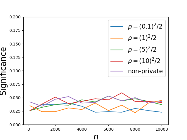
(a) Significance for testing a linear relationship. $x_{i}\sim\mathcal{N}(0.5,1)$, $y_{i}\sim 0\cdot x_{i}+\mathcal{N}(0,0.001^{2})$. $\Delta=2$.

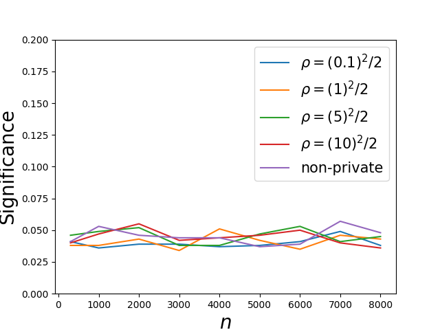
(b) Significance for testing a linear relationship. $x_{i}\sim\mathcal{N}(0.5,1)$, $y_{i}\sim 0\cdot x_{i}+\mathcal{N}(0,0.35^{2})$. $\Delta=2$.

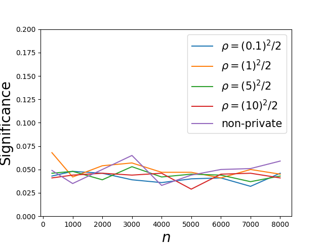
(c) Significance for testing a linear relationship. $x_{i}\sim\mathcal{N}(0.5,1)$, $y_{i}\sim 0\cdot x_{i}+\mathcal{N}(0,1)$. $\Delta=2$.

Figure 1:

Evaluating Power for Varying the Noise in the Dependent Variable: For Figures 2(a), 2(b), and 2(c), we set the true slope to 1. We then vary the noise in the dependent variable. That is, for the general linear model, $Y\sim\mathcal{N}(X\beta,\sigma_{e}^{2}I_{n\times n})$, we vary $\sigma_{e}$. The following values of $\sigma_{e}$ are considered: $\{0.001,0.35,1\}$.

In Figure 2(a), we generally see that compared to higher values of $\sigma_{e}$ (Figures 2(b) and 2(c)), the power is relatively low. We believe this occurs because when $\sigma_{e}$ is small, its DP estimate is more likely to be less than 0, in which case we fail to reject the null (even when the alternative is true). This generally leads to a reduction in the power.

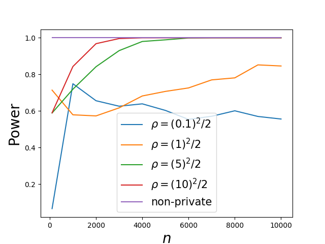
(a) Power for testing a linear relationship. $x_{i}\sim\mathcal{N}(0.5,1)$, $y_{i}\sim 1\cdot x_{i}+\mathcal{N}(0,0.001^{2})$. $\Delta=2$.

(b) Power for testing a linear relationship. $x_{i}\sim\mathcal{N}(0.5,1)$, $y_{i}\sim 1\cdot x_{i}+\mathcal{N}(0,0.35^{2})$. $\Delta=2$.

(c) Power for testing a linear relationship. $x_{i}\sim\mathcal{N}(0.5,1)$, $y_{i}\sim 1\cdot x_{i}+\mathcal{N}(0,1)$. $\Delta=2$.

Figure 2:

Evaluating Power for Varying Slopes: Figures 3(a), 3(b) show the power of the linear test for slopes of 0.1, 1. We generally see that the larger the slope, the higher the power of the DP tests.

(a) Power for testing a linear relationship.
$x_{i}\sim\mathcal{N}(0.5,1)$, $y_{i}\sim 0.1\cdot x_{i}+\mathcal{N}(0,0.35^{2})$. $\Delta=2$.

(b) Power for testing a linear relationship.
$x_{i}\sim\mathcal{N}(0.5,1)$, $y_{i}\sim 1\cdot x_{i}+\mathcal{N}(0,0.35^{2})$. $\Delta=2$.

Figure 3:

Evaluating the Significance while Varying the Distribution of the Independent Variable: For Figures 4(a), 4(b), and 4(c), we set the standard deviation of the noise dependent variable to 0.35. We then vary the distribution of the independent variable — while maintaining the variance — to take on one of the following:

1. Normal: with mean 0.5 and variance 1/12.

2. Uniform: between 0 and 1 (variance of 1/12).

3. Exponential: with scale of $1/\sqrt{12}$.

We observe that the significance is still preserved even though, in our DP testers, the null distribution is simulated via a normal distribution.

(a) Significance for testing a linear relationship. Normal Distribution on $X$.

(b) Significance for testing a linear relationship. Uniform Distribution on $X$.

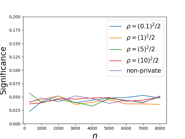
(c) Significance for testing a linear relationship. Exponential Distribution on $X$.

Figure 4:

6.1.2 Bootstrap Confidence Intervals

Using the duality between confidence interval estimation and hypothesis testing, we can construct hypothesis tests for testing a linear relationship based on DP confidence interval procedures. Specifically, we compare the $F$-statistic linear relationship tester to the tester that uses DP confidence intervals. See Section B for more details on the experimental framework of the DP bootstrap confidence intervals. Algorithm 6 summarizes the approach for testing that builds on DP confidence intervals.

In Figure 5(a), we present experimental results for the significance level of Algorithm 6 compared to Algorithm 1 instantiated with the DP $F$-statistic. As we see, Algorithm 6 achieves the target significance level. In Figure 5(b), we also present experimental results for the power of Algorithm 6 compared to Algorithm 1. We see that Algorithm 6 has less power than Algorithm 1. This observation is more pronounced for less concentrated distributions (i.e., uniform) on the independent variable. See Figure 6(b). This might be due to the, sometimes excessive, width of the confidence interval produced by the bootstrap interval (in order to ensure coverage under the null hypothesis).

Figures 5(a), 5(b), 6(a), and 6(b) show results averaged out over 2000 trials. The dashed lines correspond to the bootstrap confidence interval approach (denoted CI) while the solid lines are for the $F$-statistic (denoted $F$-stat).

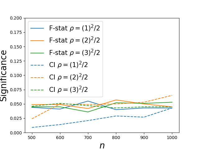
(a) Significance for $F$-statistic versus confidence interval approach. $x_{i}\sim\mathcal{N}(0.5,1)$, $y_{i}\sim 0\cdot x_{i}+\mathcal{N}(0,0.35^{2})$. $\Delta=2$.

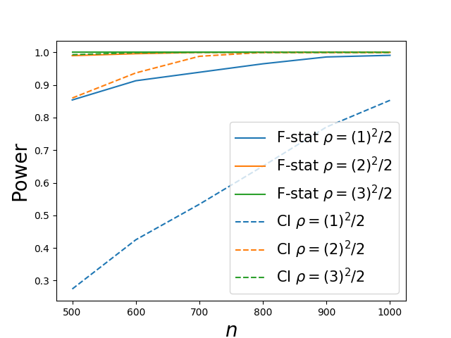
(b) Power for $F$-statistic versus confidence interval approach. $x_{i}\sim\mathcal{N}(0.5,1)$, $y_{i}\sim 1\cdot x_{i}+\mathcal{N}(0,0.35^{2})$. $\Delta=2$.

Figure 5:

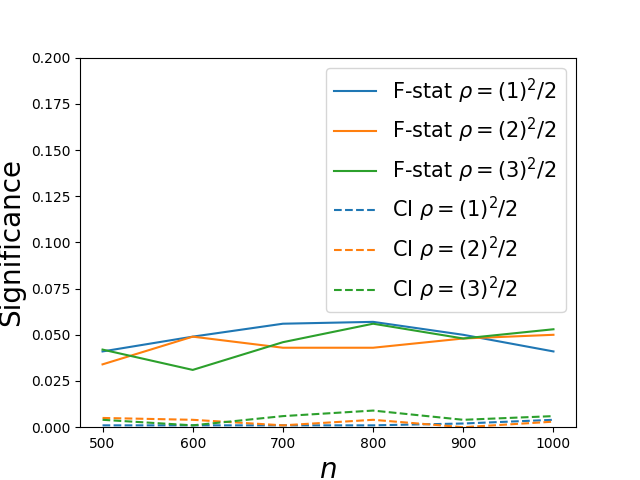
(a) Significance for $F$-statistic versus confidence interval approach. $x_{i}\sim\text{Unif}[0,1]$, $y_{i}\sim 0\cdot x_{i}+\mathcal{N}(0,0.35^{2})$. $\Delta=2$.

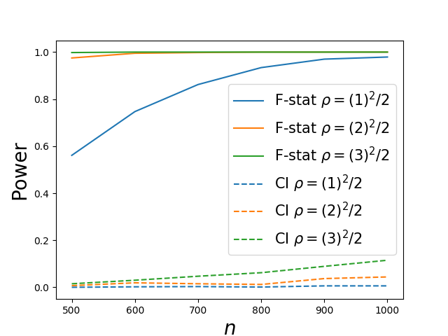
(b) Power for $F$-statistic versus confidence interval approach. $x_{i}\sim\text{Unif}[0,1]$, $y_{i}\sim 1\cdot x_{i}+\mathcal{N}(0,0.35^{2})$.
$\Delta=2$.

Figure 6:

6.1.3 Bernoulli Tester

The DP Bernoulli tester has a higher power than the DP $F$-statistic when the slope is large or the privacy-loss parameter is small; otherwise the DP $F$-statistic performs better. We vary the slope from 0.01 up to 1. As the slope gets smaller, the performance gap between the $F$-statistic and the Bernoulli tester gets larger. Figures 8(a) and 8(b) show the power of the DP $F$-statistic compared to the DP Bernoulli tester for the problem of testing a linear relationship. The significance levels of the Bernoulli tester are shown in Figures 7(a) and 7(b).

The results are averaged out over 1000 trials. For the figures illustrating the power, dashed lines correspond to the Bernoulli testing approach (denoted Bern) while the solid lines are for the $F$-statistic (denoted $F$-stat).

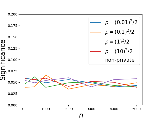
(a) Significance for testing for a fair coin.
$n$ observations are generated from $\text{Bern}(1/2)$.

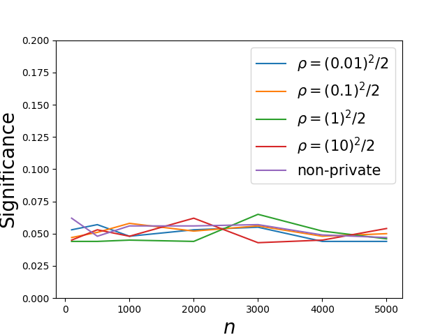
(b) Significance for linear relationship testing via Bernoulli testing approach. $x_{i}\sim\mathcal{N}(0.5,1)$, $y_{i}\sim 0\cdot x_{i}+\mathcal{N}(0,1)$. $\Delta=2$.

Figure 7:

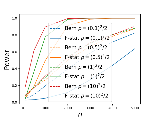
(a) Power for $F$-statistic versus Bernoulli testing approach. $x_{i}\sim\mathcal{N}(0.5,1)$, $y_{i}\sim 0.1\cdot x_{i}+\mathcal{N}(0,1)$. $\Delta=2$.

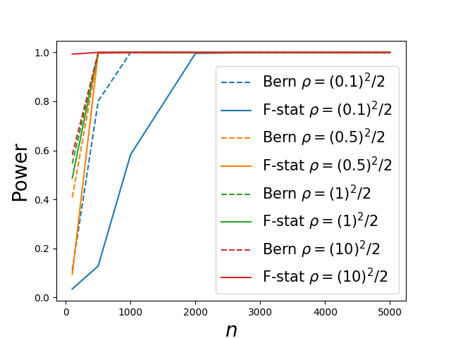
(b) Power for $F$-statistic versus Bernoulli testing approach. $x_{i}\sim\mathcal{N}(0.5,1)$, $y_{i}\sim 0.5\cdot x_{i}+\mathcal{N}(0,1)$. $\Delta=2$.

Figure 8:

6.2 Testing Mixture Models on Synthetic Data

6.2.1 $F$-Statistic

We evaluate the $F$-statistic DP mixture model test on synthetically generated data. We vary parameters such as: the fraction of data in each group and the slopes used to generate data for each group. Let $\beta_{1},\beta_{2}$ denote the slopes of the two groups.

Evaluating the Significance: Like in the DP linear model tester, we also see that we achieve the target significance levels, on average, for all values of $\rho$. In Figures 9(a), 9(b), and 9(c), we vary the noise in the dependent variable. In Figures 10(a), 10(b), and 10(c), we vary the fraction of group sizes, using either a 1/8, 1/4, or 1/2 fraction for the first group. We see that the more unbalanced splits tend to have lower significance levels.

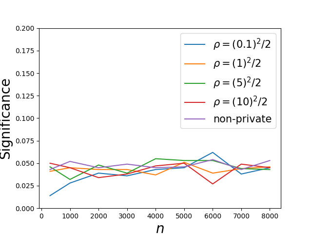
(a) Significance for testing mixtures. Equal-sized groups. $x_{i}\sim\mathcal{N}(0.5,1)$, $y_{i}\sim 1\cdot x_{i}+\mathcal{N}(0,0.01^{2})$ for Group 1. $y_{i}\sim 1\cdot x_{i}+\mathcal{N}(0,0.01^{2})$ for Group 2.

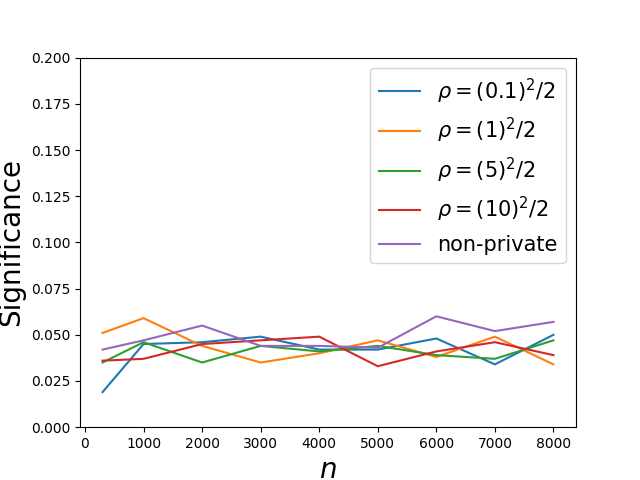
(b) Significance for testing mixtures. Equal-sized groups. $x_{i}\sim\mathcal{N}(0.5,1)$, $y_{i}\sim 1\cdot x_{i}+\mathcal{N}(0,0.35^{2})$ for Group 1. $y_{i}\sim 1\cdot x_{i}+\mathcal{N}(0,0.35^{2})$ for Group 2.

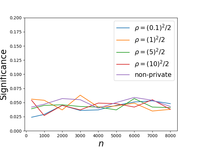
(c) Significance for testing mixtures. Equal-sized groups. $x_{i}\sim\mathcal{N}(0.5,1)$, $y_{i}\sim 1\cdot x_{i}+\mathcal{N}(0,1)$ for Group 1. $y_{i}\sim 1\cdot x_{i}+\mathcal{N}(0,1)$ for Group 2.

Figure 9:

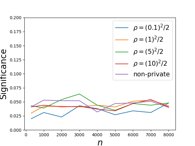
(a) Significance for testing mixtures. 1/8th vs. 7/8th splits. $x_{i}\sim\mathcal{N}(0.5,1)$, $y_{i}\sim 1\cdot x_{i}+\mathcal{N}(0,0.35^{2})$ for Group 1. $y_{i}\sim 1\cdot x_{i}+\mathcal{N}(0,0.35^{2})$ for Group 2.

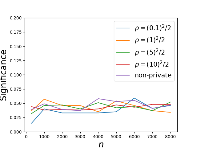
(b) Significance for testing mixtures. 1/4th vs. 3/4th splits. $x_{i}\sim\mathcal{N}(0.5,1)$, $y_{i}\sim 1\cdot x_{i}+\mathcal{N}(0,0.35^{2})$ for Group 1. $y_{i}\sim 1\cdot x_{i}+\mathcal{N}(0,0.35^{2})$ for Group 2.

(c) Significance for testing mixtures. Equal-sized groups. $x_{i}\sim\mathcal{N}(0.5,1)$, $y_{i}\sim 1\cdot x_{i}+\mathcal{N}(0,0.35^{2})$ for Group 1. $y_{i}\sim 1\cdot x_{i}+\mathcal{N}(0,0.35^{2})$ for Group 2.

Figure 10:

Power while Varying the Group Size Fraction: Let $n$ be the total number of datapoints and $n_{1},n_{2}$ be the number of points in groups 1 and 2 respectively. We vary the fraction of points in group 1: $n_{1}/n$. Setting the slopes of each group to $\beta_{1}=-1$ and $\beta_{2}=1$, we vary this fraction so that $n_{1}/n\in\{1/8,1/4,1/2\}$. For Figure 11(a), we set the group sizes to be equal. For Figure 11(b), we set the group sizes to be $n/4,3n/4$. And last, for Figure 11(c), the group sizes are $n/8,7n/8$.

Generally, the more even the group size fractions are, the higher the power of the DP test for testing mixtures in the general linear model.

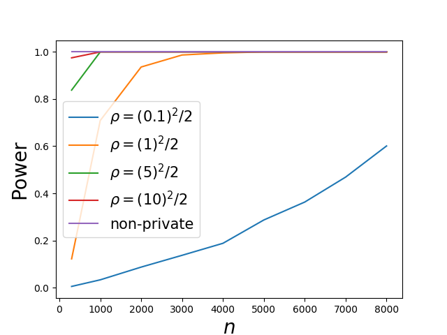
(a) Power for testing mixtures. 1/8th vs. 7/8th splits. $x_{i}\sim\mathcal{N}(0.5,1)$, $y_{i}\sim-1\cdot x_{i}+\mathcal{N}(0,0.35^{2})$ for Group 1. $y_{i}\sim 1\cdot x_{i}+\mathcal{N}(0,0.35^{2})$ for Group 2.

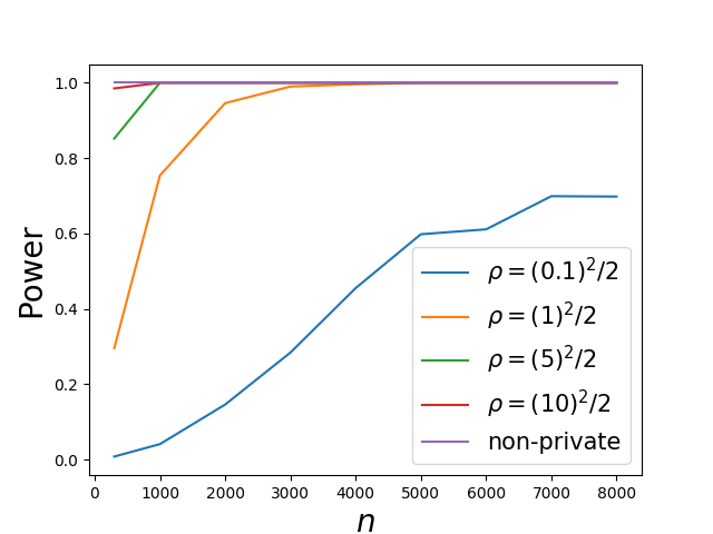
(b) Power for testing mixtures. 1/4th vs. 3/4th splits. $x_{i}\sim\mathcal{N}(0.5,1)$, $y_{i}\sim-1\cdot x_{i}+\mathcal{N}(0,0.35^{2})$ for Group 1. $y_{i}\sim 1\cdot x_{i}+\mathcal{N}(0,0.35^{2})$ for Group 2.

(c) Power for testing mixtures. Equal-sized groups. $x_{i}\sim\mathcal{N}(0.5,1)$, $y_{i}\sim-1\cdot x_{i}+\mathcal{N}(0,1)$ for Group 1. $y_{i}\sim 1\cdot x_{i}+\mathcal{N}(0,1)$ for Group 2.

Figure 11:

Power while Varying the Difference Between Slopes in Each Group: Let $\beta_{1},\beta_{2}$ correspond to the slopes for groups 1 and 2. We vary $|\beta_{1}-\beta_{2}|$. Generally, we see that the larger $|\beta_{1}-\beta_{2}|$ is, the higher the power of the test. In Figures 12(a), 12(b) we vary the slope in the two groups and observe the aforementioned phenomena.

(a) Power for testing mixtures. Equal-sized groups. $x_{i}\sim\mathcal{N}(0.5,1)$, $y_{i}\sim-0.1\cdot x_{i}+\mathcal{N}(0,0.35^{2})$ for Group 1. $y_{i}\sim 0.1\cdot x_{i}+\mathcal{N}(0,0.35^{2})$ for Group 2.

(b) Power for testing mixtures. Equal-sized groups. $x_{i}\sim\mathcal{N}(0.5,1)$, $y_{i}\sim-1\cdot x_{i}+\mathcal{N}(0,0.35^{2})$ for Group 1. $y_{i}\sim 1\cdot x_{i}+\mathcal{N}(0,0.35^{2})$ for Group 2.

Figure 12:

Power while Varying the Noise in the Dependent Variable: We also vary $\sigma_{e}$. We generally see that the smaller it is, the smaller the power. We conjecture that this happens because we err on the side of failing to reject the null if the DP estimate of $\sigma_{e}$ becomes $\leq 0$, which is more likely to happen if $\sigma_{e}$ is small. In Figures 13(a), 13(b),and 13(c) we see this phenomenon.

(a) Power for testing mixtures. Equal-sized groups. $x_{i}\sim\mathcal{N}(0.5,1)$, $y_{i}\sim-1\cdot x_{i}+\mathcal{N}(0,0.01^{2})$ for Group 1. $y_{i}\sim 1\cdot x_{i}+\mathcal{N}(0,0.01^{2})$ for Group 2.

(b) Power for testing mixtures. Equal-sized groups. $x_{i}\sim\mathcal{N}(0.5,1)$, $y_{i}\sim-1\cdot x_{i}+\mathcal{N}(0,0.35^{2})$ for Group 1. $y_{i}\sim 1\cdot x_{i}+\mathcal{N}(0,0.35^{2})$ for Group 2.

(c) Power for testing mixtures. Equal-sized groups. $x_{i}\sim\mathcal{N}(0.5,1)$, $y_{i}\sim-1\cdot x_{i}+\mathcal{N}(0,1)$ for Group 1. $y_{i}\sim 1\cdot x_{i}+\mathcal{N}(0,1)$ for Group 2.

Figure 13:

6.2.2 Nonparametric Tests via Kruskal-Wallis

We now proceed to show results for comparing the mixture models based on Kruskal-Wallis (KW) to the parametric $F$-statistic method.

Evaluating the Significance: The KW methods, on average, achieve the target significance levels for all values of $\rho$ as illustrated in Figures 14(a) and 14(b), where we vary the noise in the dependent variable.

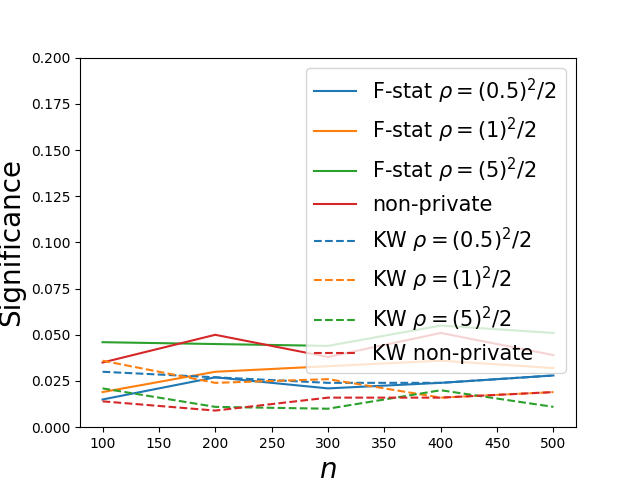
(a) Significance for testing mixtures. Equal-sized groups. $x_{i}\sim\mathcal{N}(0.5,0.1)$, $y_{i}\sim 1\cdot x_{i}+\mathcal{N}(0,0.35^{2})$ for Group 1. $y_{i}\sim 1\cdot x_{i}+\mathcal{N}(0,0.35^{2})$ for Group 2.

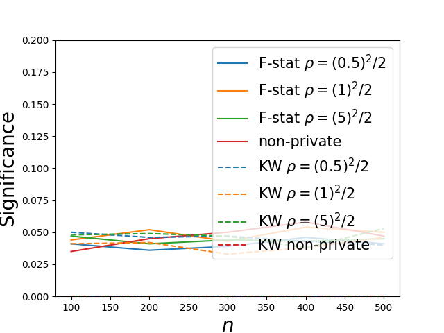
(b) Significance for testing mixtures. Equal-sized groups. $x_{i}\sim\mathcal{N}(0.5,1)$, $y_{i}\sim 1\cdot x_{i}+\mathcal{N}(0,1)$ for Group 1. $y_{i}\sim 1\cdot x_{i}+\mathcal{N}(0,1)$ for Group 2.

Figure 14:

Evaluating the Power as we Increase the Difference in Slopes: We see that the the KW method outperforms the $F$-statistic method on small datasets. But as the difference in slopes between the two groups increases, the $F$-statistic method does better and begins to outperform the KW method. See Figures 15(a) and  15(b).

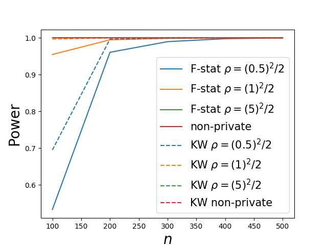
(a) Power for testing mixtures. Equal-sized groups. $x_{i}\sim\mathcal{N}(0.5,1)$, $y_{i}\sim-1\cdot x_{i}+\mathcal{N}(0,1)$ for Group 1. $y_{i}\sim 1\cdot x_{i}+\mathcal{N}(0,1)$ for Group 2.

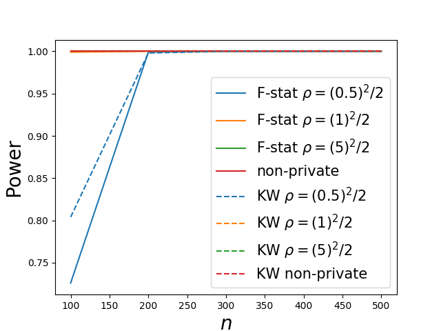
(b) Power for testing mixtures. Equal-sized groups. $x_{i}\sim\mathcal{N}(0.5,1)$, $y_{i}\sim-1\cdot x_{i}+\mathcal{N}(0,1)$ for Group 1. $y_{i}\sim 5\cdot x_{i}+\mathcal{N}(0,1)$ for Group 2.

Figure 15:

Evaluating the Power as we Increase the Variance of the Independent Variable: In Figures 16(a) and 16(b), we see that the $F$-statistic method outperforms the KW method when the variance of the independent variable is much larger (10x) than previously.

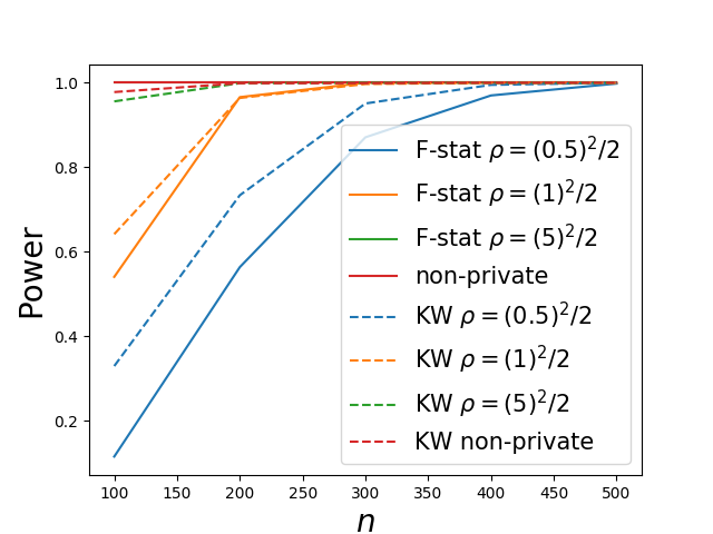
(a) Power for Kruskal-Wallis versus the $F$-statistic. $x_{i}\sim\mathcal{N}(0.5,1)$, $y_{i}\sim-1\cdot x_{i}+\mathcal{N}(0,1)$ for Group 1. $y_{i}\sim 1\cdot x_{i}+\mathcal{N}(0,1)$ for Group 2.

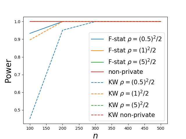
(b) Power for Kruskal-Wallis versus the $F$-statistic. $x_{i}\sim\mathcal{N}(0.5,10)$, $y_{i}\sim-1\cdot x_{i}+\mathcal{N}(0,1)$ for Group 1. $y_{i}\sim 1\cdot x_{i}+\mathcal{N}(0,1)$ for Group 2.

Figure 16:

6.3 Testing on Opportunity Insights Data

The Opportunity Insights (OI) team gave us simulated data for census tracts from the following states in the United States: Idaho, Illinois, New York, North Carolina, Texas, and Tennessee. The dependent and independent variables are the child and parent national income percentiles, respectively. For the linear tester, a rejection of the null hypothesis implies that there is a relationship between the parent and child income percentiles. For the mixture model tester, it implies that there is more than one linear relationship in the data which suggests that more granular data is needed for analysis on the data. The groups of data fed to the mixture model tester are conglomeration of one or more tracts.

Some of these states have a small number of datapoints. For example, within Illinois, there are tracts with just $n=39$ datapoints. For the Illinois dataset, there are $n=219,594$ datapoints that are subdivided into $3,108$ census tracts. The North Carolina and Texas datasets consists of datapoints subdivided into $2,156$ and $5,187$ census tracts respectively. We will focus on data from North Carolina (NC), and Texas (TX) and experimentally evaluate $\mathbb{P}[\text{reject null}]$, the probability of rejecting the null hypothesis over the randomness of the DP algorithms. We run our tests on some census tracts in these states showing how these measures fair as the privacy parameter is relaxed. For the experiments below, from each state, we randomly and uniformly select: (i) a single tract; (ii) 10 randomly selected tracts and concatenate; and (iii) 50 randomly selected tracts and concatenate. Then we test for the presence of a (non-zero) linear relationship. The concatenation could result in hundreds or thousands of points.

Our tests are evaluated on the OI data. We have not included the test based on Kruskal-Wallis as our current implementation is, at the moment, relatively computationally inefficient to evaluate on such large datasets. See above synthetic data experiments for comparison of Kruskal-Wallis to the $F$-statistic method. Figures 17(a), and 17(b) show the probability of rejecting the null as we increase the parameter $\rho$ when using the DP linear tester. Figures 18(a), and 18(b) show the corresponding results for the $F$-stat based DP mixture model tester. We see that for the small-sized datasets tend to have a small chance of rejecting the null while larger ones have a higher chance.

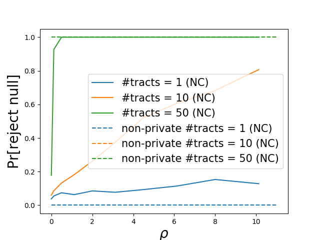
(a) $\mathbb{P}[\text{reject null}]$ for testing a linear relationship in NC. $\Delta=2$.

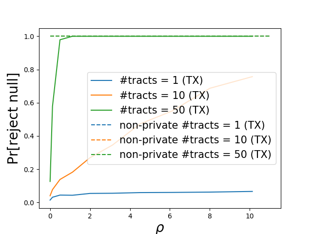
(b) $\mathbb{P}[\text{reject null}]$ for testing a linear relationship in TX. $\Delta=2$.

Figure 17:

(a) $\mathbb{P}[\text{reject null}]$ for testing for mixtures in NC. $\Delta=2$.

(b) $\mathbb{P}[\text{reject null}]$ for testing for mixtures in TX. $\Delta=2$.

Figure 18:

6.4 Testing on UCI Bike Dataset

We use the UCI bike dataset  [28] with 17,389 instances. For this dataset, we test for a linear relationship between the “temp” (normalized temperature in Celsius) and “hr” (hour between 0 and 23) attributes. The null hypothesis is that there is no linear relationship between the “temp” and “hr” attributes. Without privacy, the linear relationship tester based on the $F$-statistic rejects the null. In Table 1, we show the probability of Algorithm 1 rejecting the null as we vary the privacy parameter. We can observe that for almost all—except for the smallest setting of $\rho$—privacy parameters, $\mathbb{P}[\text{reject null}\mid p\%\text{ data}]$ (probability of rejecting the null, given $p\%$ of the dataset) for the private test matches that of the non-private test.

$\rho$	0.005	0.125	0.5	1.125	2.0	3.125	4.5	6.125	8.0	10.125	non-DP
$\mathbb{P}[\text{reject null}\mid 100\%\text{ data}]$	1.0	1.0	1.0	1.0	1.0	1.0	1.0	1.0	1.0	1.0	1.0
$\mathbb{P}[\text{reject null}\mid 10\%\text{ data}]$	0.85	1.0	1.0	1.0	1.0	1.0	1.0	1.0	1.0	1.0	1.0

Table 1: $\mathbb{P}[\text{reject null}]$ for testing for a linear relationship between temperature and time (in hours).

While we show that our methods can run on real-world datasets, the synthetically generated datasets give a lot more information on the behavior of the tests.

7 Conclusion

We have developed differentially private hypothesis tests for testing a linear relationship in data and for testing for mixtures in linear regression models. We also show that the DP $F$-statistic converges to the asymptotic distribution of the non-private $F$-statistic. Through experiments, we show that our Monte Carlo tests achieve significance that is less than the target significance level across a wide variety of experiments. Furthermore, our tests generally have a high power, getting higher as we increase the dataset size and/or relax the privacy parameter. Even on small datasets (in the hundreds) with small slopes, our tests retain the small significance while having a good power. We have provided formal statements for the DP $F$-statistic in the asymptotic regime. We leave to future work the task of theoretically analyzing the procedures in the non-asymptotic regime.

Experimental evaluation is done on simulated data for the Opportunity Atlas tool, UCI datasets, and on synthetic datasets of varying distributions on the independent variable (normal, exponential, and uniform).

8 Other Acknowledgements

We are grateful to Mark Fleischer (of the U.S. Census Bureau) for many helpful comments and suggestions that improved the presentation of this work. We thank Isaiah Andrews, Jordan Awan, Cynthia Dwork, Cecilia Ferrando, Kosuke Imai, Gary King, Po-Ling Loh, Santiago Olivella, Neil Shephard, Adam Smith, Thomas Steinke, Soichiro Yamauchi, and seminar participants of the Harvard econometrics workshop for helpful discussions related to this work. Finally, we thank anonymous reviewers for helpful comments.

Appendix A $F$-Statistic for the General Linear Model

The proofs in this section rely on insights from  [36]. In fact, Theorem A.2 can be seen as a special case of Theorem 14.11 in [36] where, under the null hypothesis, the projection onto $\omega_{0}$ results in $\beta^{N}$ and, under the alternative hypothesis, the projection onto $\omega$ results in $\beta$.

We present the main test statistic we will use for hypothesis testing. This statistic is equivalent to the generalized likelihood ratio test statistic and can be written as

$$T=\left(\frac{n-r}{r-q}\right)\frac{\mathopen{\|}Y-X\hat{\beta}^{N}\mathclose{\|}^{2}-\mathopen{\|}Y-X\hat{\beta}\mathclose{\|}^{2}}{\mathopen{\|}Y-X\hat{\beta}\mathclose{\|}^{2}}=\left(\frac{n-r}{r-q}\right)\frac{\mathopen{\|}X\hat{\beta}-X\hat{\beta}^{N}\mathclose{\|}^{2}}{\mathopen{\|}Y-X\hat{\beta}\mathclose{\|}^{2}},$$ (21)

where $\hat{\beta}^{N},\hat{\beta}$ are the least squares estimates under the null and alternative hypothesis respectively.

The vectors $Y-X\hat{\beta}$ and $X\hat{\beta}-X\hat{\beta}^{N}$ can be shown to be orthogonal, so that $\mathopen{\|}Y-X\hat{\beta}^{N}\mathclose{\|}^{2}=\mathopen{\|}Y-X\hat{\beta}\mathclose{\|}^{2}+\mathopen{\|}X\hat{\beta}-X\hat{\beta}^{N}\mathclose{\|}^{2}$ by the Pythagorean theorem [36].

Lemma A.1 (Weak Law of Large Numbers, see [36]).

Let $Y_{1},\ldots,Y_{n}$ be i.i.d. random variables with mean $\mu$. Then

$$\frac{1}{n}\sum_{i=1}^{n}Y_{i}=\bar{Y}_{n}\xrightarrow{P}\mu,$$

provided that $\mathbb{E}[|Y_{i}|]<\infty$.

Theorem A.2.

For every $n\in{\mathbb{N}}$ with $n>r$, let $X=X_{n}\in{\mathbb{R}}^{n\times p}$ be the design matrix. Under the general linear model $Y=Y_{n}\sim\mathcal{N}(X_{n}\beta,\sigma_{e}^{2}I_{n\times n})$,

$$T=T_{n}\sim F_{r-q,n-r}(\eta_{n}^{2}),\quad\eta_{n}^{2}=\frac{\mathopen{\|}X_{n}\beta-X_{n}\beta^{N}\mathclose{\|}^{2}}{\sigma_{e}^{2}},$$

where $F_{n,m}$ is the $F$-distribution with parameters $n$, $m$, $\beta^{N}=\mathbb{E}[\hat{\beta}^{N}]$, $q$ is the dimension of $\omega_{0}$, and $r$ is the dimension of $\omega$ with $0\leq q<r$.

Furthermore,

1. $$\mathopen{\|}Y_{n}-X_{n}\hat{\beta}\mathclose{\|}^{2}\sim\mathcal{X}^{2}_{n-r}\sigma_{e}^{2},\quad\mathopen{\|}X_{n}\hat{\beta}-X_{n}\hat{\beta}^{N}\mathclose{\|}^{2}\sim\mathcal{X}^{2}_{r-q}(\eta_{n}^{2})\sigma_{e}^{2}.$$

2. If there exists $\eta\in{\mathbb{R}}$ such that $\frac{\mathopen{\|}X_{n}\beta-X_{n}\beta^{N}\mathclose{\|}^{2}}{\sigma_{e}^{2}}\rightarrow\eta^{2}$, then

   $$T=T_{n}\sim F_{r-q,n-r}(\eta_{n}^{2})\xrightarrow{D}\frac{\chi^{2}_{r-q}(\eta^{2})}{r-q}.$$

3. We have

   $$\frac{\mathopen{\|}Y_{n}-X_{n}\hat{\beta}\mathclose{\|}^{2}}{n-r}\xrightarrow{P}\sigma_{e}^{2}.$$

The values $\beta=\mathbb{E}[\hat{\beta}],\beta^{N}=\mathbb{E}[\hat{\beta}^{N}]$ are the expected values of our parameter estimates under the alternative and null hypotheses respectively.

Proof of Lemma A.2.

First, define $\Omega_{0}=\{X\beta\,:\,\beta\in{\mathbb{R}}^{p},\beta\in\omega_{0}\}$ (for null hypothesis) and $\Omega=\text{span}\{c_{1},\ldots,c_{p}\}=\{X\beta\,:\,\beta\in{\mathbb{R}}^{p},\beta\in\omega\}$ (for alternative) where $c_{1},\ldots,c_{p}$ are the columns of $X$. Write $Y=\sum_{i=1}^{n}Z_{i}v_{i}$, where $v_{1},\ldots,v_{n}$ is an orthonormal basis chosen so that $v_{1},\ldots,v_{r}$ spans $\Omega$ (so that $v_{r+1},\ldots,v_{n}$ lies in $\Omega^{\perp}$) and $v_{1},\ldots,v_{q}$ spans $\Omega_{0}$.

For all $i\in[n]$, we can find $Z_{i}\in{\mathbb{R}}^{n}$ by introducing an $n\times n$ matrix $O$ with columns $v_{1},\ldots,v_{n}$. As a result, $O$ is an orthogonal matrix (i.e., $O^{T}O=OO^{T}=I$ since $O$ is a square matrix) such that $Z=O^{T}Y$ (or $Y=OZ$).

As before $Y=X\beta+e$, where $e\sim\mathcal{N}(0,\sigma_{e}^{2}I_{n\times n})$. As a result, $Z=O^{T}(X\beta+e)=O^{T}X\beta+O^{T}e$. If we define $\tau=O^{T}X\beta$ and $e^{*}=O^{T}e$, then $Z=\tau+e^{*}$. And because $\mathbb{E}[e^{*}]=\mathbb{E}[O^{T}e]=O^{T}\mathbb{E}[e]=0$ and $\mathrm{cov}(e^{*})=\mathrm{cov}(O^{T}e)=O^{T}\mathrm{cov}(e)O=O^{T}(\sigma_{e}^{2}I)O=\sigma_{e}^{2}I$, $e^{*}\sim\mathcal{N}(0,\sigma_{e}^{2}I_{n\times n})$. As a result,

$$Z\sim\mathcal{N}(\tau,\sigma_{e}^{2}I_{n\times n}).$$

Next, since $c_{1},\ldots,c_{p}$ denotes the columns of the design matrix $X$, $X\beta=\sum_{i=1}^{p}\beta_{i}c_{i}$ and

$$\tau=O^{T}X\beta=\begin{pmatrix}v_{1}^{T}\\ v_{2}^{T}\\ \vdots\\ v_{n}^{T}\\ \end{pmatrix}\sum_{i=1}^{p}\beta_{i}c_{i}=\begin{pmatrix}\sum_{i=1}^{p}\beta_{i}v_{1}^{T}c_{i}\\ \sum_{i=1}^{p}\beta_{i}v_{2}^{T}c_{i}\\ \vdots\\ \sum_{i=1}^{p}\beta_{i}v_{n}^{T}c_{i}\\ \end{pmatrix}.$$

And because $c_{1},\ldots,c_{p}$ all lie in $\Omega$ and $v_{r+1},\ldots,v_{n}$ in $\Omega^{\perp}$, we have $v^{T}_{k}c_{i}=0$ for all $k>r$. Then, $\tau_{r+1}=\cdots=\tau_{n}=0.$

Additionally, because $\tau=O^{T}X\beta$,

$$X\beta=O\tau=(v_{1}\cdots v_{n})\begin{pmatrix}\tau_{1}\\ \tau_{2}\\ \vdots\\ \tau_{r}\\ 0\\ \vdots\\ 0\end{pmatrix}=\sum_{i=1}^{r}\tau_{i}v_{i}.$$

Essentially, we established a one-to-one relation between points $X\beta\in\Omega$ and $(\tau_{1},\ldots,\tau_{r})\in{\mathbb{R}}^{r}$.

Now, since $Z\sim\mathcal{N}(\tau,\sigma_{e}^{2}I_{n\times n})$, $Z_{1},\ldots,Z_{n}$ are independent and $Z_{i}\sim\mathcal{N}(\tau_{i},\sigma_{e}^{2})$ for all $i\in[n]$. Furthermore, $\tau_{r+1}=\cdots=\tau_{n}=0$.

Then since $X\beta=\sum_{i=1}^{r}\tau_{i}v_{i}$, $X\hat{\beta}=\sum_{i=1}^{r}Z_{i}v_{i}$ and $X\hat{\beta}^{N}=\sum_{i=1}^{q}Z_{i}v_{i}$.

As a result, we get

$$\mathopen{\|}Y-X\hat{\beta}\mathclose{\|}^{2}=\mathopen{\|}\sum_{i=r+1}^{n}Z_{i}v_{i}\mathclose{\|}^{2}=\sum_{i=r+1}^{n}\sum_{j=r+1}^{n}Z_{i}Z_{j}v_{i}^{T}v_{j}=\sum_{i=r+1}^{n}Z_{i}^{2},$$

which follows since for all $i\neq j$, $v^{T}_{i}v_{j}=0$ and for $i=j$, $v^{T}_{i}v_{j}=1$. Also, since $\tau_{r+1}=\cdots=\tau_{n}=0$, $Z_{i}\sim\sigma_{e}\mathcal{N}(\tau_{i},1)$, $\mathopen{\|}Y-X\hat{\beta}\mathclose{\|}^{2}\sim\mathcal{X}^{2}_{n-r}\sigma_{e}^{2}$.

Similarly,

$$\mathopen{\|}Y-X\hat{\beta}^{N}\mathclose{\|}^{2}=\sum_{i=q+1}^{n}Z_{i}^{2}.$$

Then by Equation (21),

$$T=\frac{\frac{1}{r-q}\sum_{i=q+1}^{r}Z_{i}^{2}}{\frac{1}{n-r}\sum_{i=r+1}^{n}Z_{i}^{2}}=\frac{\frac{1}{r-q}\sum_{i=q+1}^{r}(Z_{i}/\sigma_{e})^{2}}{\frac{1}{n-r}\sum_{i=r+1}^{n}(Z_{i}/\sigma_{e})^{2}}.$$

The variables $Z_{i}$ are independent and because $Z_{i}/\sigma_{e}\sim\mathcal{N}(\tau_{i}/\sigma_{e},1)$, using properties of the (non-central) chi-squared distribution,

$$\sum_{i=q+1}^{r}\left(\frac{Z_{i}}{\sigma_{e}}\right)^{2}\sim\chi^{2}_{r-q}(\eta_{n}^{2}),\quad\eta_{n}^{2}=\sum_{i=q+1}^{r}\frac{\tau_{i}^{2}}{\sigma_{e}^{2}}.$$

As a corollary, $\mathopen{\|}X\hat{\beta}-X\hat{\beta}^{N}\mathclose{\|}^{2}\sim\mathcal{X}^{2}_{r-q}(\eta_{n}^{2})\sigma_{e}^{2}$.

Also, since $\tau_{i}=0$ for $i=r+1,\ldots,n$, $Z_{i}/\sigma_{e}\sim\mathcal{N}(0,1)$ for $i=r+1,\ldots,n$. As a result, $\sum_{i=r+1}^{n}(Z_{i}/\sigma_{e})^{2}\sim\chi^{2}_{n-r}$.

By definition of the noncentral $F$-distribution, we have $T\sim F_{r-q,n-r}(\eta_{n}^{2})$ where $\eta_{n}^{2}=\sum_{i=q+1}^{r}\frac{\tau_{i}^{2}}{\sigma_{e}^{2}}$.

We know that $X\beta=\mathbb{E}[X\hat{\beta}]=\sum_{i=1}^{r}\tau_{i}v_{i}$ and $X\beta^{N}=\mathbb{E}[X\hat{\beta}^{N}]=\sum_{i=1}^{q}\tau_{i}v_{i}$. As a result, $X\beta-X\beta^{N}=\sum_{i=q+1}^{r}\tau_{i}v_{i}$ so that

$$\mathopen{\|}X\beta-X\beta^{N}\mathclose{\|}^{2}=\sum_{i=q+1}^{r}\tau_{i}^{2}.$$

This completes the proof of the distribution of $T$.

In the limit, by Lemma A.3

$$T_{n}=F_{r-q,n-r}(\eta_{n}^{2})\xrightarrow{D}\frac{\chi^{2}_{r-q}(\eta^{2})}{r-q}.$$

Finally, we have established that

$$\frac{\mathopen{\|}Y_{n}-X_{n}\hat{\beta}\mathclose{\|}^{2}}{n-r}\sim\frac{\mathcal{X}^{2}_{n-r}\sigma_{e}^{2}}{n-r}.$$

Applying the weak law of large numbers (Lemma A.1), $\frac{\chi^{2}_{n-r}}{n-r}\xrightarrow{P}1$. As a result,

$$\frac{\mathopen{\|}Y_{n}-X_{n}\hat{\beta}\mathclose{\|}^{2}}{n-r}\xrightarrow{P}\sigma_{e}^{2}.$$

∎

Lemma A.3.

Let $X\sim F_{n,m}(\lambda)$ and $Y=\lim_{m\rightarrow\infty}nX$. Then $Y\sim\chi^{2}_{n}(\lambda)$.

Proof.

By definition of the $F$-distribution, $X=\frac{N/n}{M/m}$, where $N\sim\mathcal{X}^{2}_{n}(\lambda)$ and $M\sim\mathcal{X}^{2}_{m}$ are independent random variables.

For mutually independent $\chi^{2}_{1}$ random variables $Y_{1},\ldots,Y_{m}$,

$$M=\frac{Y_{1}+\cdots+Y_{m}}{m}.$$

By the weak law of large numbers (Lemma A.1),

$$\frac{M}{m}\xrightarrow{P}\mathbb{E}[Y_{1}]=1.$$

As a result, by Slutsky’s Theorem (Theorem 5.6),

$$\lim_{m\rightarrow\infty}nX=\lim_{m\rightarrow\infty}\frac{N}{M/m}=N\sim\mathcal{X}^{2}_{n}(\lambda).$$

∎

Appendix B Duality Between Testing and Interval Estimation

In this section, we expand on the relationship between interval or region estimation (i.e., confidence interval estimation) and hypothesis testing. We present a general formulation, which can be specialized to linear regression. Previous work (e.g., [29]) examines the generation of confidence intervals for differentially private parametric inference. Our work focuses on hypothesis testing.

As before, for some unknown parameter $\theta\in\Omega,Z\sim P_{\theta}$ is the observed data. Also let $f:\Omega\rightarrow{\mathbb{R}}$ be a function on the parameter space (i.e., for linear regression, we can compute functions of the slope and/or intercept).

Definition B.1 (Confidence Region).

A (random) set $S(Z)$ is a $1-\alpha$ confidence region for a (function of a) parameter $f(\theta)$ if

$$\mathbb{P}_{\theta}[f(\theta)\in S(Z)]\geq 1-\alpha,\quad\forall\theta\in\Omega.$$

A confidence region is, essentially, a multi-dimensional generalization of a confidence interval.

Definition B.2 (Acceptance Region).

For every $f_{0}\in{\mathbb{R}}$, $A(f_{0})$ is the acceptance region for a nonrandomized level $\alpha$ test of

$$H_{0}:f(\theta)=f_{0}\,\text{ vs. }\,H_{1}:f(\theta)\neq f_{0}.$$

$A(f_{0})$ denotes the range of values that would lead to acceptance of the null hypothesis, when the null is true, where for the level $\alpha$ test,

$$\mathbb{P}_{\theta}[Z\in A(f(\theta))]\geq 1-\alpha,\quad\forall\theta\in\Omega.$$

Define the following function:

$$S(z)=\{f_{0}\,:\,\exists\theta_{0}\text{ s.t. }f_{0}=f(\theta_{0})\text{ and }z\in A(f_{0})\}.$$

Then $f(\theta)\in S(Z)\iff Z\in A(f(\theta))$ which implies that

$$\mathbb{P}_{\theta}(f(\theta)\in S(Z))=\mathbb{P}_{\theta}(Z\in A(f(\theta)))\geq 1-\alpha.$$

We have established that $S(Z)$ is, thus, a $1-\alpha$ confidence region for $f$. Essentially, we have shown that we can construct confidence regions from a family of nonrandomized tests.

For any function $f:\Omega\rightarrow{\mathbb{R}}$ and $f_{0}=f(\theta_{0})$, we could seek to obtain a $1-\alpha$ confidence region $S(Z)$ for the parameter $f_{0}$ (e.g., the mean or median).

Now, consider a test $\phi$ defined by

$$\phi(z)=\begin{cases}1&\mbox{if }f_{0}\notin S(z)\\ 0&\mbox{otherwise}\end{cases}.$$

Then if $f(\theta)=f_{0}$, then

$$\mathbb{E}_{\theta}\phi =\mathbb{P}_{\theta}[f_{0}\notin S(Z)]$$ (22)

$$=\mathbb{P}_{\theta}[f(\theta)\notin S(Z)]\leq\alpha.$$ (23)

This test has level at most $\alpha$ for testing

$$H_{0}:f(\theta)=f_{0}\,\text{ vs. }\,H_{1}:f(\theta)\neq f_{0}.$$

Then if the coverage probability for $S(Z)$ is exactly $1-\alpha$, then

$$\mathbb{P}_{\theta}[f(\theta)\in S(Z)]=1-\alpha,\quad\forall\theta\in\Omega,$$

so that $\phi$ will have level of exactly $\alpha$.

To summarize, we have shown that we can: (1) Construct confidence regions from a family of nonrandomized tests. (2) Construct a family of nonrandomized tests from a $1-\alpha$ confidence region.

Since (nontrivial) DP tests are randomized, to apply the duality framework, we could de-randomize by giving the DP procedure the random bits to be used for DP. Or we can also define the DP procedure as a family of nonrandomized tests.

We can still turn DP procedures for confidence region estimation into procedures for testing although, as we show below, the power of the corresponding tests is likely to be very low if the area of the confidence regions are too large.

B.1 More Details on Experimental Evaluation of DP Confidence Intervals

We now proceed to construct a hypothesis test based on DP parametric bootstrap confidence intervals (e.g., using the work of [29]). Then we will experimentally compare to our linear relationship tester based on the DP $F$-statistic.

Suppose that $\theta$ is the set of parameters (e.g., standard deviation of the dependent and independent variables) and $f=f(\theta)$ is the estimation target (e.g., the slope in the dataset). The goal is to obtain a $1-\alpha$ confidence interval $[\hat{a}_{n},\hat{b}_{n}]$ for $f(\theta)$ via an end-to-end differentially private procedure. In other words, we want

$$\mathbb{P}\left[\hat{a}_{n}\leq f(\theta)\leq\hat{b}_{n}\right]=1-\alpha,$$

where the probability is taken over both $\theta$ and $f$.

Because of the randomized nature of (non-trivial) DP procedures, the finite-sample coverage of the interval might not exactly be close to $1-\alpha$. Ferrando, Wang, and Sheldon [29] show the consistency of these intervals (in the large-sample, asymptotic regime).

Algorithm 6 follows the same framework as Algorithm 1, except that instead of simulating test statistics under the null hypothesis, the goal is to calculate a confidence interval for the slope. $P_{(\tilde{\theta}_{0},\tilde{\theta}_{1})}$ denotes the distribution from which we shall generate our bootstrap samples and from which a confidence interval can be estimated. For example, for taking bootstrap samples for the slope, $P_{(\tilde{\theta}_{0},\tilde{\theta}_{1})}$ would approximately be distributed as $\mathcal{N}(\tilde{\beta}_{1},\frac{\widetilde{S^{2}}}{\widetilde{\textrm{nvar}}})$ where $\widetilde{\textrm{nvar}}=n\cdot\widetilde{\overline{x^{2}}}-n\cdot\tilde{x}^{2}$ and $\widetilde{S^{2}}$ is as defined in Algorithm 2. Note that a crucial difference between tests based on the parametric bootstrap confidence intervals and our tests is the following: our tests only use $\tilde{\theta}_{0}$, a subset of the estimated DP statistics, to simulate the null distribution and decide to reject the null while the other approach uses $(\tilde{\theta}_{0},\tilde{\theta}_{1})$ to decide to reject the null.

The target slope is $b$. For example, if we seek to test for a linear relationship, we set $b=0$ since under the null hypothesis, the slope will be 0. DPStats is a $\rho$-zCDP procedure for estimating DP sufficient statistics for a parametric model. In Algorithm 6, $(s_{(l)},s_{(r)})$ is the parametric bootstrap confidence interval for the slopes under the null hypothesis.

Data: $X\in{\mathbb{R}}^{n\times p};Y\in{\mathbb{R}}^{n}$

Input: $n\text{ (dataset size)};\rho\text{ (privacy-loss parameter)};\alpha\text{ (target significance)};b\text{ (target slope)}$

$(\tilde{\theta}_{0},\tilde{\theta}_{1})=\texttt{DPStats}(X,Y,n,\rho)$

if $\tilde{\theta}_{0}=\tilde{\theta}_{1}=\perp$ then

       return Fail to Reject the null

 

Select $K>1/\alpha$

for $k=1\ldots K$ do

      

      Sample slope $s_{k}\sim P_{(\tilde{\theta}_{0},\tilde{\theta}_{1})}$

 

Sort $s_{(1)}\leq\cdots\leq s_{(K)}$

 

Set $l=\lceil(K+1)(\alpha/2)\rceil$

Set $r=\lceil(K+1)(1-\alpha/2)\rceil$

if  $b\notin(s_{(l)},s_{(r)})$  then

       return Reject the null

else

       return Fail to Reject the null

Algorithm 6 DP Test Framework via Parametric Bootstrap Confidence Intervals.

Without privacy, by Lemma 5.3, under the null hypothesis, we know that the slopes will be distributed as the following distribution: $\hat{\beta}_{1}\sim\mathcal{N}\left(\beta,\frac{\sigma_{e}^{2}}{n\cdot\widehat{\sigma^{2}_{x}}}\right)\sim\mathcal{N}\left(0,\frac{\sigma_{e}^{2}}{n\cdot\widehat{\sigma^{2}_{x}}}\right)$. Even as $n$ increases and as we take fresh samples of $\hat{\beta}_{1}$, the parametric bootstrap confidence interval around $\hat{\beta}_{1}$ gets smaller and more concentrated around the true value 0. We expect to observe similar behavior when applying DP.

Appendix C Experimental Framework for Monte Carlo Evaluation

In Algorithm 7, we present a generic procedure showing how we obtain significance and power on our experimental evaluation of our DP tests. $\mathrm{EstimateRejectionProb}$ is a meta-procedure that uses $\mathrm{DataSampler}$ to sample a dataset $D$ either from the null or alternative distribution we are testing. Then it runs $\mathrm{MonteCarloTester}$ to decide whether to reject or fail to reject the null. $\mathrm{MonteCarloTester}$ can be any of the private Monte Carlo tests defined above or their non-private versions. The fraction of times (amongst $M$ trials) a reject decision is returned is estimated and can be used to calculate the significance or the power of the test.

$\mathrm{DataSampler}$:

This procedure is used to sample from a user-specified distribution for testing the null or the alternative hypothesis. For example, for two groups $(X_{1},Y_{1})$ and $(X_{2},Y_{2})$ with slopes $\beta_{1}$ and $\beta_{2}$ respectively, the user could specify $\beta_{1}=\beta_{2}$ as parameters to the data sampler. Other parameters include the size of the groups, the noise distribution in the dependent or independent variable, and so on.

$\mathrm{MonteCarloTester}$:

Examples of this procedure are instantiations of Algorithm 1.

$\mathrm{CompareAlgorithms}$:

For user-specified data samplers and Monte Carlo test procedures, this procedure (Algorithm 8) collates significance and power (to be plotted, for example).

Input: $\mathrm{DataSampler};\mathrm{MonteCarloTester};M(\#trials)$

$r=0$

for $m=1,\ldots,M$ do

       $D\leftarrow\mathrm{DataSampler}()$

      if $\mathrm{MonteCarloTester}(D)$ = Reject the null then

             $r=r+1$

      

// Compute empirical probability that the test rejects

return $r/M$

Algorithm 7 $\mathrm{EstimateRejectionProb}$: Meta-Procedure for Estimating significance and power.

Input: $\mathrm{DataSamplerList};\mathrm{MonteCarloTesterList};M(\#trials)$

$R=[]$

for $\mathrm{DataSampler}\in\mathrm{DataSamplerList}$ do

      

      for $\mathrm{MonteCarloTester}\in\mathrm{MonteCarloTesterList}$ do

             $e=\mathrm{EstimateRejectionProb}(\mathrm{DataSampler},\mathrm{MonteCarloTester},M)$

            Append $(\mathrm{DataSampler},\mathrm{MonteCarloTester},M,e)$ to $R$

      

return $R$

Algorithm 8 $\mathrm{CompareAlgorithms}$: Compares statistical performance of DP tests.

References

- ACFT [19] Jayadev Acharya, Clément L. Canonne, Cody Freitag, and Himanshu Tyagi. Test without trust: Optimal locally private distribution testing. In AISTATS, pages 2067–2076, 2019.
- ADKR [19] Maryam Aliakbarpour, Ilias Diakonikolas, Daniel Kane, and Ronitt Rubinfeld. Private testing of distributions via sample permutations. In NeurIPS, pages 10877–10888, 2019.
- ADR [18] Maryam Aliakbarpour, Ilias Diakonikolas, and Ronitt Rubinfeld. Differentially private identity and equivalence testing of discrete distributions. In ICML, pages 169–178, 2018.
- AKM [19] Isaiah Andrews, Toru Kitagawa, and Adam McCloskey. Inference on winners. Working Paper 25456, National Bureau of Economic Research, January 2019.
- AM [20] Marco Avella-Medina. Privacy-preserving parametric inference: A case for robust statistics. Journal of the American Statistical Association, 0(0):1–15, 2020.
- AMS+ [22] Daniel Alabi, Audra McMillan, Jayshree Sarathy, Adam Smith, and Salil Vadhan. Differentially private simple linear regression. Proc. Priv. Enhancing Technol., 2022.
- AS [20] Jordan Alexander Awan and Aleksandra Slavkovic. Differentially private inference for binomial data. Journal of Privacy and Confidentiality, 10(1), Jan. 2020.
- ASZ [18] Jayadev Acharya, Ziteng Sun, and Huanyu Zhang. Differentially private testing of identity and closeness of discrete distributions. In NeurIPS, pages 6879–6891, 2018.
- BDR [10] Philipp Bleninger, Jörg Drechsler, and Gerd Ronning. Remote data access and the risk of disclosure from linear regression: An empirical study. In PSD, volume 6344 of Lecture Notes in Computer Science, pages 220–233. Springer, 2010.
- BRMC [17] Andr’es F. Barrientos, J. Reiter, Ashwin Machanavajjhala, and Yan Chen. Differentially private significance tests for regression coefficients. Journal of Computational and Graphical Statistics, 28:440 – 453, 2017.
- BS [16] Mark Bun and Thomas Steinke. Concentrated differential privacy: Simplifications, extensions, and lower bounds. In TCC, pages 635–658, 2016.
- BS [19] Garrett Bernstein and Daniel R. Sheldon. Differentially private bayesian linear regression. In NeurIPS, pages 523–533, 2019.
- CBRG [18] Zachary Campbell, Andrew Bray, Anna M. Ritz, and Adam Groce. Differentially private ANOVA testing. In ICDIS, pages 281–285, 2018.
- CF [19] Raj Chetty and John N. Friedman. A practical method to reduce privacy loss when disclosing statistics based on small samples. American Economic Review Papers and Proceedings, 109:414–420, 2019.
- CFH+ [18] Raj Chetty, John N Friedman, Nathaniel Hendren, Maggie R Jones, and Sonya R Porter. The opportunity atlas: Mapping the childhood roots of social mobility. Working Paper 25147, National Bureau of Economic Research, October 2018.
- CH [12] Kamalika Chaudhuri and Daniel J. Hsu. Convergence rates for differentially private statistical estimation. In Proceedings of the 29th International Conference on Machine Learning, ICML 2012, Edinburgh, Scotland, UK, June 26 - July 1, 2012, 2012.
- CHJP [19] Raj Chetty, Nathaniel Hendren, Maggie R Jones, and Sonya R Porter. Race and Economic Opportunity in the United States: an Intergenerational Perspective*. The Quarterly Journal of Economics, 135(2):711–783, 12 2019.
- CKM+ [19] Clément L. Canonne, Gautam Kamath, Audra McMillan, Adam D. Smith, and Jonathan Ullman. The structure of optimal private tests for simple hypotheses. In STOC, pages 310–321, 2019.
- CKS+ [19] Simon Couch, Zeki Kazan, Kaiyan Shi, Andrew Bray, and Adam Groce. Differentially private nonparametric hypothesis testing. In CCS, pages 737–751, 2019.
- CKS [20] Clément L. Canonne, Gautam Kamath, and Thomas Steinke. The discrete gaussian for differential privacy. In NeurIPS, 2020.
- CWZ [20] T. Tony Cai, Yichen Wang, and Linjun Zhang. The cost of privacy in generalized linear models: Algorithms and minimax lower bounds. CoRR, abs/2011.03900, 2020.
- DKM+ [06] Cynthia Dwork, Krishnaram Kenthapadi, Frank McSherry, Ilya Mironov, and Moni Naor. Our data, ourselves: Privacy via distributed noise generation. In EUROCRYPT, pages 486–503, 2006.
- DL [09] Cynthia Dwork and Jing Lei. Differential privacy and robust statistics. In STOC, pages 371–380, 2009.
- DMNS [06] Cynthia Dwork, Frank McSherry, Kobbi Nissim, and Adam D. Smith. Calibrating noise to sensitivity in private data analysis. In TCC, pages 265–284, 2006.
- DSSU [17] Cynthia Dwork, Adam Smith, Thomas Steinke, and Jonathan Ullman. Exposed! a survey of attacks on private data. Annual Review of Statistics and Its Application, 4(1):61–84, 2017.
- Edg [11] Eugene S. Edgington. Randomization Tests, pages 1182–1183. Springer Berlin Heidelberg, Berlin, Heidelberg, 2011.
- EKST [19] G. Evans, G. King, Margaret Schwenzfeier, and Abhradeep Thakurta. Statistically valid inferences from privacy protected data. 2019.
- FG [14] Hadi Fanaee-T and João Gama. Event labeling combining ensemble detectors and background knowledge. Prog. Artif. Intell., 2(2-3):113–127, 2014.
- FWS [21] Cecilia Ferrando, Shufan Wang, and Daniel Sheldon. Parametric bootstrap for differentially private confidence intervals. CoRR, abs/2006.07749, 2021.
- GLRV [16] Marco Gaboardi, Hyun-Woo Lim, Ryan M. Rogers, and Salil P. Vadhan. Differentially private chi-squared hypothesis testing: Goodness of fit and independence testing. In ICML, pages 2111–2120, 2016.
- Gut [13] A. Gut. Probability: A Graduate Course. Springer Texts in Statistics. Springer New York, 2013.
- HJ [12] Roger A. Horn and Charles R. Johnson. Matrix Analysis. Cambridge University Press, 2 edition, 2012.
- HR [11] P.J. Huber and E.M. Ronchetti. Robust Statistics. Wiley Series in Probability and Statistics. Wiley, 2011.
- HTF [09] Trevor Hastie, Robert Tibshirani, and Jerome H. Friedman. The Elements of Statistical Learning: Data Mining, Inference, and Prediction, 2nd Edition. Springer Series in Statistics. Springer, 2009.
- Hub [64] Peter J. Huber. Robust Estimation of a Location Parameter. The Annals of Mathematical Statistics, 35(1):73 – 101, 1964.
- Kee [10] R.W. Keener. Theoretical Statistics: Topics for a Core Course. Springer Texts in Statistics. Springer New York, 2010.
- KOV [16] Peter Kairouz, Sewoong Oh, and Pramod Viswanath. Extremal mechanisms for local differential privacy. J. Mach. Learn. Res., 17:17:1–17:51, 2016.
- Lei [11] Jing Lei. Differentially private m-estimators. In NeurIPS, pages 361–369, 2011.
- Mir [17] Ilya Mironov. Rényi differential privacy. In CSF, pages 263–275, 2017.
- RK [17] Ryan Rogers and Daniel Kifer. A new class of private chi-square hypothesis tests. In AISTATS, pages 991–1000, 2017.
- SGG+ [19] Marika Swanberg, Ira Globus-Harris, Iris Griffith, Anna M. Ritz, Adam Groce, and Andrew Bray. Improved differentially private analysis of variance. Proc. Priv. Enhancing Technol., 2019(3):310–330, 2019.
- She [17] Or Sheffet. Differentially private ordinary least squares. In ICML, pages 3105–3114, 2017.
- She [18] Or Sheffet. Locally private hypothesis testing. In ICML, pages 4612–4621, 2018.
- Sur [20] Ananda Theertha Suresh. Robust hypothesis testing and distribution estimation in hellinger distance. CoRR, abs/2011.01848, 2020.
- Swe [97] Latanya Sweeney. Weaving technology and policy together to maintain confidentiality. The Journal of Law, Medicine & Ethics, 25(2-3):98–110, 1997.
- TC [16] Christine Task and Chris Clifton. Differentially private significance testing on paired-sample data. In Proceedings of the 2016 SIAM International Conference on Data Mining, Miami, Florida, USA, May 5-7, 2016, pages 153–161. SIAM, 2016.
- Vaa [98] A. W. van der Vaart. Asymptotic Statistics. Cambridge Series in Statistical and Probabilistic Mathematics. Cambridge University Press, 1998.
- Wan [18] Yu-Xiang Wang. Revisiting differentially private linear regression: optimal and adaptive prediction & estimation in unbounded domain. In UAI, pages 93–103, 2018.
- WLK [15] Yue Wang, Jaewoo Lee, and Daniel Kifer. Differentially private hypothesis testing, revisited. CoRR, abs/1511.03376, 2015.