A Unitarity Approach to Two-Loop All-Plus Rational Terms

Abstract

We present a calculation of the rational terms in two-loop all-plus gluon amplitudes using $D$-dimensional unitarity. We use a conjecture of separability of the two loops, and then a simple generalization of one-loop $D$-dimensional unitarity to perform calculations. We compute the four- and five-point rational terms analytically, and the six- and seven-point ones numerically. We find agreement with previous calculations of Dalgleish, Dunbar, Godwin, Jehu, Perkins, and Strong. For a special subleading-color amplitude, we compute the eight- and nine-point results numerically, and find agreement with an all-$n$ conjecture of Dunbar, Perkins, and Strong.

SAGEX-22-26-E

MITP-22-040

I Introduction

Increasing integrated luminosity at the Large Hadron Collider (LHC) in the coming decade will drive experimenters’ search for physics beyond the Standard Model (SM). The LHC will not be surging into a new energy domain, but will be sensitive to ever-fainter discrepancies from SM predictions. The greater sensitivity will emerge both from increased statistics and from a better understanding of systematic uncertainties. Greater experimental sensitivity does not suffice, however, in order to find small deviations from theoretical expectations. We also need higher-precision calculations, in particular in perturbative QCD, in order to reduce theoretical uncertainties.

The current frontier for perturbative QCD calculations is at next-to-next-to-leading order (NNLO), where one may broadly hope that results will reduce these latter uncertainties to below a few percent. Because of renormalization-scale sensitivity in leading-order (LO) calculations, next-to-leading order (NLO) calculations provide the first truly quantitative predictions, and NNLO is then the first order at which theoretical uncertainties can be assessed quantitatively.

Many results, primarily for $2\rightarrow 1$ and $2\rightarrow 2$ processes, are already available at NNLO (and sometimes beyond). The generalization of NNLO calculations to multijet processes requires developments of several aspects, most notably of two-loop amplitudes and of infrared-regulation techniques. In this article, we explore a technique for computing certain contributions to a simple class of two-loop Yang–Mills amplitudes, the so-called “all-plus” amplitudes, with all external gluons of identical helicity.

These amplitudes are simpler than general two-loop amplitudes. At tree level, they vanish. This vanishing can be proven diagrammatically, or understood as the consequence of a supersymmetry identity [1].

As a result, the one-loop amplitudes are free of ultraviolet and infrared divergences, and indeed are purely rational in the external spinors [2, 3, 4, 5, 6]. In turn, two-loop amplitudes have singularities in dimensional regularization of the same degree as general one-loop amplitudes. The polylogarithmic weights in their finite terms are the same as those in one-loop amplitudes. The two-loop all-plus amplitudes are in a sense intermediate in complexity between one-loop amplitudes and general two-loop amplitudes. In this respect, they are a good laboratory for exploring aspects of Yang–Mills amplitudes beyond what is probed in ${\cal N}=4$ supersymmetric amplitudes. These amplitudes may also be a portal to exploring hidden connections between different theories: at one loop, there is an intriguing connection [7, 8] between the all-plus amplitude and the simplest ${\cal N}=4$ super-Yang–Mills amplitude, scattering all gluons but two of like helicity (MHV). Furthermore, for four and five gluons in the planar limit, the leading transcendental weight parts of all-plus amplitudes at two loops (and three loops for four gluons) have been shown to be dual to those of ${\cal N}=4$ Wilson loops with Lagrangian insertions at one lower loop order [9]. This duality is conjectured to hold for any loop order.

The four-point all-plus amplitude at two loops was computed long ago by Bern, Dixon, and one of the authors [10]. Much later, Badger, Frellesvig, and Zhang (BFZ) computed [11] the leading-color part of the five-point all-plus amplitude (partly analytically and partly numerically); Badger, Mogull, Ochirov, and O’Connell computed the full integrand [12] for the five-point amplitude; Gehrmann, Henn, and Lo Presti gave an analytic form of the leading-color part [13]. More recently, Abreu, Dormans, Febres Cordero, Ita, Page, and Zeng gave an analytic form for the planar amplitude [14] by reconstructing an expression from a numerical calculation, while Badger, Chicherin, Gehrmann, Heinrich, Henn, Peraro, Wasser, Zhang and Zoia gave an analytic form of the full amplitude by integrating the earlier integrand [15].

There are also results at three loops: the leading-color four-gluon amplitude was computed by Jin and Luo [16], while the full, non-planar QCD result was recently computed by Caola, Chakraborty, Gambuti, von Manteuffel, and Tancredi [17].

The structure of the all-plus amplitude at two loops, as we shall review in the next section, has made it possible for Dunbar, Jehu, and Perkins (DJP) [18] to compute the polylogarithmic terms for an arbitrary number of external gluons at leading color. In addition, Dalgleish, Dunbar, Godwin, Jehu, Perkins, and Strong [19, 20, 21, 22, 23, 24, 25] have also computed the rational terms in the five- and six-point amplitudes at leading and subleading color, as well as the leading-color seven-point amplitude. They made use of recursive techniques to do so. Dunbar, Perkins, and Strong (DPS) presented an all-$n$ conjecture for a special subleading-color amplitude [33]. Badger, Mogull and Peraro (BMP) [26] have also computed the leading-color five- and six-point amplitudes through a reconstruction of the integrand. In addition, they presented a conjecture for the all-$n$ integrand on which we shall rely in our calculations.

This article is organized as follows. In the next section, we review general aspects of all-plus amplitudes and present the separability conjecture along with the dimensional decompositions we use. In Sect. III, we discuss the color structure and generating sets of unitarity cuts. We look at the required tree-level amplitudes in Sect. IV, and discuss the Mathematica implementation of our calculations in Sect. VI. We present the four-point calculation in detail in Sect. V, and an overview of higher-point calculations in Sect. VII. We make concluding remarks in Sect. VIII. In the appendices, we detail our conventions (App. A); list the massive-scalar tree amplitudes we use (App. B); present a current-based alternative calculation of contact contributions to four-scalar amplitudes (App. C); present an alternate form of the seven-point subleading-color single-trace amplitude (App. D); give an $n$-point momentum-twistor parametrization (App. E); and list the one-loop expressions for integral coefficients we use in our calculations (App. F). We also attach a set of auxiliary files, containing the Mathematica packages implementing the methods presented in this paper; lists of the unitarity cuts required for the rational parts of all partial amplitudes with up to nine gluons; and analytic expressions for the five-point rational parts derived using our automated code.

II Review, Separability, and Dimensional Reconstruction

We know from considerations of infrared and ultraviolet divergences that two-loop all-plus amplitudes have no singularities stronger than $1/\epsilon^{2}$ in dimensional regularization, and that the singular terms are proportional to the one-loop amplitude. What about the finite, polylogaritmic terms? We can imagine looking at four-dimensional cuts to extract information about them. For example, localizing both loop momenta in a double box in four dimensions, following the prescriptions of ref. [27], we see that there is no possible helicity assignment of internal legs that yields a non-vanishing coefficient for the integral. While the analogous procedure is not known for other integrals, one would presumably be drawn to a similar conclusion from examining integrands [26].

Even with ordinary unitarity, once we cut one of the two loops, we are left with too simple a function to cut another loop. If we fully localize one of the loop integrals, performing a quadruple cut on it, we will find a product of rational functions, as illustrated in Fig. 1. One of these functions will be the one-loop all-plus amplitude, a rational functions of the spinor variables just like the tree-level amplitudes at the other three corners.

Figure 1: A four-dimensional quadruple cut of one of the loops in the leading-color two-loop all-plus amplitude. The all-plus configuration requires the cut to be either of the one-mass or easy two-mass box type. In addition, the second loop can only appear as a one-loop all-plus amplitude.

This implies that the calculation of the polylogarithmic terms follows a one-loop recipe faithfully: one computes the coefficients of one-loop box, triangle, and bubble integrals following the prescriptions of refs. [28, 29, 30], or alternatively, the integrand approach of ref. [31]. This is the procedure that DJP carried out in ref. [18], and Dunbar, Godwin, Jehu, and Perkins in refs. [32].

Four-dimensional cuts do not suffice, however, in order to compute the rational terms. Dunbar, Godwin, Jehu, Perkins, and Strong made use of recursion relations to compute them through the seven-point amplitude [32, 33, 34]. We will explore a different approach, using $D$-dimensional unitarity, to do so.

II.1 General Structure of All-Plus Amplitudes

At tree level, all-plus amplitudes vanish in Yang–Mills theories. We can see this in a number of ways. One approach relies on the BCFW on-shell recursion relations [28, 35]. The three-point all-plus amplitude vanishes in pure Yang–Mills with a dimensionless coupling. The factorization channel(s) in the four-point amplitude necessarily involve this three-point amplitude, and hence likewise vanish. At higher points, each factorization channel necessarily involves a lower-point all-plus amplitude, and hence this argument continues inductively to all multiplicity.

The tree-level vanishing simplifies loop amplitudes. At one-loop, amplitudes can be written in a form exposing their universal singular structure [37, 38, 39, 40],

$$A^{(1)}=A^{(0)}I^{(1)}+F^{(1)}+\mathcal{O}(\epsilon)\,.$$ (1)

Here, $I^{(1)}$ is a universal function of the Lorentz invariants, which through double and single poles in $\epsilon$ summarizes the singular structure of the amplitudes. The next term, $F^{(1)}$, is of $\mathcal{O}(\epsilon^{0})$. The vanishing of $A^{(0)}$ immediately implies the finiteness of the one-loop amplitudes. In general, $F^{(1)}$ contains logarithms and polylogarithms in addition to rational functions of the spinor variables. In the all-plus amplitudes, it contains only rational terms. The absence of logarithms and polylogarithms can be understood in ordinary unitarity in four dimensions [38, 41]. Perform an ordinary cut in any channel of a color-ordered amplitude. In the $K_{1\ldots j}$ channel, for example, we find for the discontinuities,

$$A^{(1)}_{n} (1^{+},\ldots,n^{+})\big{|}_{s_{1\ldots j}\textrm{\ cut}}=$$ (2)

$$\sum_{h_{a,b}=\pm}\int d^{4}\textrm{LIPS}(k_{a},k_{b})\;A^{(0)}(1^{+},\ldots,j^{+},k_{a}^{h_{a}},k_{b}^{h_{b}})$$

$$\hskip 122.34685pt\times A^{(0)}((j+1)^{+},\ldots,n^{+},(-k_{b})^{-h_{b}},(-k_{a})^{h_{a}})\,,$$

where $d\textrm{LIPS}$ is the Lorentz-invariant phase-space measure. This cut is illustrated in Fig. 2.

      

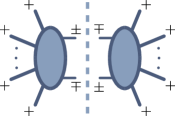
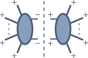
Figure 2: An ordinary cut of a one-loop all-plus amplitude

All terms contain either a single-minus or all-plus tree amplitude, both of which vanish. Thus, one-loop all-plus amplitudes are free of discontinuities, and have to be entirely rational. For the leading-color partial amplitude, general expressions for these rational terms were conjectured in ref. [4] by demanding correct collinear factorization,

$$A^{(1)}(1^{+}\mathellipsis n^{+})=-\frac{1}{3}\frac{\sum_{1\leq i<j<k<l\leq n}\mathinner{\langle{i|jkl|i}]}}{\mathinner{\langle{12}\rangle}\mathinner{\langle{23}\rangle}\mathellipsis\mathinner{\langle{(n-1)n}\rangle}\mathinner{\langle{n1}\rangle}}+\mathcal{O}(\epsilon)\,,$$ (4)

a form which was later proven in ref. [6]. The subleading-color amplitudes at one-loop can always be obtained from the leading-color ones through color relations [36]. Compact forms for them are also known [34],

$$A^{(1)}_{n:2}(1^{+};2^{+}\mathellipsis n^{+}) =-\frac{\sum_{2\leq i<j\leq n}\mathinner{[{1|ij|1}]}}{\mathinner{\langle{23}\rangle}\mathinner{\langle{34}\rangle}\mathellipsis\mathinner{\langle{(n-1)n}\rangle}\mathinner{\langle{n2}\rangle}}\,,$$ (5)

$$A^{(1)}_{n:r}(1^{+}\mathellipsis(r-1)^{+};r^{+}\mathellipsis n^{+}) =-2\frac{s_{1\mathellipsis(r-1)}^{2}}{\mathinner{\langle{12}\rangle}\mathinner{\langle{23}\rangle}\mathellipsis\mathinner{\langle{(r-1)1}\rangle}\mathinner{\langle{r(r+1)}\rangle}\mathellipsis\mathinner{\langle{nr}\rangle}},$$ (6)

which respectively multiply the subleading color structures $\operatorname{Tr}(T^{a_{1}})\operatorname{Tr}(T^{a_{2}}\mathellipsis T^{a_{n}})$ and $\operatorname{Tr}(T^{a_{1}}\mathellipsis T^{a_{r-1}})\operatorname{Tr}(T^{a_{r}}\mathellipsis T^{a_{n}})$, where $r\geq 3$. The amplitude $A^{(1)}_{n:2}(1^{+};2^{+}\mathellipsis n^{+})$ is equivalent to the one-photon amplitude $A^{(1)}(1^{\gamma}\,2^{+}\mathellipsis n^{+})$, for which a compact all-$n$ form was provided earlier in ref. [4]. Given their finiteness and absence of branch-cuts these expressions seem more like tree-level amplitudes rather than one-loop ones.

The first computation of a two-loop all-plus amplitude was presented in refs. [10, 42, 43], which provided analytic expressions for the full-color four-gluon amplitude. For five gluons, the planar and non-planar integrands were derived in Badger, Frellesvig and Zhang (BHZ) [11] and by Badger, Mogull, Ochirov and O’Connell (BMOOC) [44] respectively, together with results from numerical integration. Analytic results for the planar amplitude were first given in ref. [13]. The full-color two-loop all-plus amplitude was then given in ref. [15].

As in the one-loop case, two-loop amplitudes can be decomposed with respect to their singularity structure [45], which leads us to a relation similar to that of eq. (1),

$$A^{(2)}=A^{(0)}I^{(2)}+A^{(1)}I^{(1)}+F^{(2)}+\mathcal{O}(\epsilon).$$ (7)

Here, $I^{(2)}$ is (like $I^{(1)}$) a universal function of the Lorentz invariants with divergences up to $\epsilon^{-4}$; $I^{(1)}$ is the same function given in eq. (1). The remainder $F^{(2)}$ is finite in dimensional regularization, and in general contains both polylogarithmic and rational terms. For all-plus amplitudes, we again find significant simplifications: the vanishing of $A^{(0)}$ and finiteness of $A^{(1)}$ allows only for divergences up to $\epsilon^{-2}$. This is the same degree of divergence that we would ordinarily expect in a one-loop amplitude. The universal behavior allows us to obtain all divergent terms in $A^{(2)}$, leaving us to compute only the finite part $F^{(2)}$.

Figure 3: Ordinary cuts in the two-loop all-plus amplitude.

We may split $F^{(2)}$ into polylogarithmic and rational parts $P^{(2)}$ and $R^{(2)}$,

$$F^{(2)}=P^{(2)}+R^{(2)}\,.$$ (8)

The polylogarithmic part $P^{(2)}$ has ordinary branch cuts, which are shown schematically for the all-plus amplitude in Fig. 3, and may therefore be computed using four-dimensional generalized unitarity. In contrast, the rational part $R^{(2)}$ does not contain such discontinuities and requires separate treatment.

II.2 Dimensional Reconstruction

In dimensional regularization, scattering amplitudes depend on the spacetime dimension $D$. Dimensional regulators come in a number of different flavors, which differ in their treatment of observed and unobserved particles, and also in how the number of states for particles with spin are continued away from four dimensions. Over the years, different variants of dimensional regularization have been used. In the conventional scheme (CDR), all particles are treated in $D$ dimensions, as are the number of states. Because the number of states for bosons and fermions continues differently, this scheme is incompatible with maintaining manifest supersymmetry; and because it requires extra polarization states even for observed particles, it is incompatible with efficient use of helicity methods.

In the so-called four-dimensional helicity scheme (FDH) and in the ’t Hooft–Veltman scheme, observed particles are treated strictly in four dimensions, while unobserved particles — those inside loops, or soft or collinear real emissions — are treated in $D$ dimensions. The dimensional reduction (DR) scheme compactifies $2\epsilon$ dimensions, thereby maintaining manifest compatibility with supersymmetry. Its use of dimensions smaller than four, however, is awkward for helicity methods beyond one loop.

In this article, we follow a modified approach originally introduced in ref. [10], and later exploited at one loop in ref. [46] and at two loops by BMP [26] to help isolate rational contributions. It introduces two distinct dimensional parameters: $D$, which controls the dimension of loop-momentum integrations, and $D_{s}$, which controls the number of states, with $D_{s}$ taken to be greater than $D$. Integrands of loop amplitudes then depend polynomially on $D_{s}$, while integrals depend in a general analytic fashion on $D$.

The value of $D_{s}$ is of course not integral. Because of the polynomial dependence, however, it is possible to reconstruct the full dependence on this parameter by sampling the integrand at a number of integer values for it. Ref. [46] showed how to do this at one loop, where the dependence is linear. At two loops, the dependence in quadratic, but we can employ the same strategy.

This allows us to avoid evaluating the tree amplitudes arising in generalized-unitarity cuts in non-integer dimensions. Instead, we are free to perform all evaluations in integer dimensions. This makes dimensional reconstruction a useful technique for both analytic computations as well as automated semi-numerical codes. It has found application in determining various one- and two-loop amplitudes in recent years [11, 44, 26, 47, 15, 48, 14, 49, 50, 51, 52, 53, 54, 55].

BMP connect [26] the rational terms in the two-loop all-plus amplitude to the integrand’s dependence on the state dimension $D_{s}$. We review their construction briefly. We also rely on the one-loop discussion [46], as well as on the $L$-loop generalization presented in ref. [56].

In pure Yang–Mills amplitudes, the $D_{s}$ dependence of loop amplitudes arises from contractions of the metric tensor $\tensor{\eta}{{}^{\mu\nu}}$ along loops. Each contraction that ultimately closes on itself generates a yields a trace $\tensor{\eta}{{}^{\mu}_{\mu}}=D_{s}$. Vector bosons carry a single index, so that an $L$-loop scattering amplitude can be written as a degree-$L$ polynomial in in $D_{s}$,

$$A_{D_{s}}^{(L)}=\sum_{j=0}^{L}\hat{A}_{j}^{\vphantom{j}}D_{s}^{j}.$$ (9)

We can determine the coefficients $\hat{A}_{i}$ by sampling the amplitude at $L+1$ different values of $D_{s}$.

Let us now discuss the constraints on the values which we can use. We begin with one-loop amplitudes, the simplest case to consider. At one loop, we can have at most a single contraction $\tensor{\eta}{{}^{\mu}_{\mu}}$, so amplitudes are linear in $D_{s}$,

$$A_{D_{s}}^{(1)}=\hat{A}_{0}^{(1)}+\hat{A}_{1}^{(1)}D_{s}\,.$$ (10)

A similar form holds for the integrand. If we evaluate the amplitude in two different integer dimensions $D_{0}$ and $D_{1}$, we can solve for the coefficients $\hat{A}_{0,1}^{(1)}$, and then write,

$$A_{D_{s}}^{(1)}=\frac{D_{s}-D_{0}}{D_{1}-D_{0}}A_{1}^{(1)}+\frac{D_{s}-D_{1}}{D_{0}-D_{1}}A_{0}^{(1)}\,,$$ (11)

in terms of the $D_{0,1}$-dimensional amplitudes $A_{0,1}^{(1)}$. A similar result holds for integrands. Choosing $D_{1}=D_{0}+1$, this expression simplifies,

$$A^{(1)}_{D_{s}}=(D_{s}-D_{0})A_{1}^{(1)}-(D_{s}-D_{1})A_{0}^{(1)}\,.$$ (12)

As we take the external momenta to be four-dimensional, we must choose $D_{0}>4$ in order to capture the entire amplitude including rational contributions. It suffices to choose $D_{0}$ large enough so that we can fully embed the loop momentum $\ell$ in a $D_{0}$-dimensional space. kinematics. At one loop, we have only one $D$-dimensional vector, and so the components beyond four dimensions can only appear in $\ell^{2}$. It can thus be embedded in five dimensions, and it suffices to choose $D_{0}=5$.

With this choice, we then have $D_{1}=6$. In the $D_{1}$-dimensional evaluation, we can use Lorentz invariance to rotate away the sixth-dimensional components of the loop momentum. We denote the four-dimensional components of the loop momentum by $\bar{\ell}$, so that in both the $D_{0}$- and $D_{1}$-dimensional evaluations, the loop momentum has a nontrivial fifth-dimensional component. Higher-dimensional components vanish.

In $D_{s}$ dimensions, gluons will have $D_{s}-2$ physical polarizations. When we cut propagators, we make use of a completeness relation to separate the $D_{s}$-dimensional metric tensor in its state sum,

$$\eta^{\mu\nu}=-\sum_{j=1}^{D_{s}-2}\varepsilon_{j}^{\mu}(\ell)\varepsilon_{j}^{\nu*}(\ell)\,.$$ (13)

Each polarization vector is attached to an amplitude on one or the other side of the cut. In generalized unitarity, all amplitudes arising from cuts will be tree amplitudes, now taken to have the cut external legs with $D_{s}$-dimensional state counting.

In the five-dimensional evaluation, we have three polarization vectors satisfying the usual conditions,

$$\eta_{\mu\nu}\varepsilon_{i}^{\mu}\varepsilon_{j}^{\nu*} =-\delta_{ij}\,,\quad\ell_{\mu}\varepsilon_{i}^{\mu} =0\,.$$ (14)

In the six-dimensional evaluation, we have four polarization states. We can choose three of them to be the same as the five-dimensional polarization states. Because we have rotated the loop momentum to have vanishing sixth component, we are free to choose the fourth and last polarization vector to point in the sixth direction, $\varepsilon_{4}^{\mu}=-\eta^{5\mu}$. (The directions are as usual labeled $0\ldots(D-1)$ in $D$ dimensions.) This vector satisfies the conditions in eq. (14). Its only nonvanishing dot product is then with itself, $\varepsilon_{4}\cdot\varepsilon_{4}$. That is, it can only appear contracted to itself by a sequence of metrics, so that it acts as though it is a scalar field. (Of course, it transforms under the color $SU(N)$ as an adjoint.) We will call it $\varphi$.

(a)

(b)

(c)

Figure 4: Feynman vertices for an adjoint scalar field: (a) the trilinear vertex $V_{3}(1_{\varphi}2_{g}3_{\varphi})$ (b) the quadrilinear vertex $V_{4}(1_{g}2_{g}3_{\varphi}4_{\varphi})$ (c) the quadrilinear vertex $V_{4}^{\mu\nu}(1_{g}2_{\varphi}3_{g}4_{\varphi})$. Solid lines represent gluons, while the dashed lines are scalars. Quartic vertices involving scalars are represented as shaded disks, where the internal lines in the disk show the flow of the scalar flavor. This will become more relevant in the multi-loop case, where there is more than one scalar.

We can derive Feynman rules for $\varphi$ from the three- and four-point gluon vertices simply by setting the Lorentz indices associated to $\varphi$ to $5$,

$$\begin{gathered}V_{3}^{\mu}(1_{\varphi}2_{g}3_{\varphi})=\frac{i}{\sqrt{2}}(k_{1}-k_{3})^{\mu}\,,\qquad V_{4}^{\mu\nu}(1_{g}2_{g}3_{\varphi}4_{\varphi})=\frac{i}{2}\eta^{\mu\nu}\,,\\ V_{4}^{\mu\nu}(1_{g}2_{\varphi}3_{g}4_{\varphi})=-i\eta^{\mu\nu}\,,\end{gathered}$$ (15)

with all other configurations yielding vanishing vertices. We also have the propagator,

$$\begin{gathered}\frac{i}{p^{2}}\,.\end{gathered}$$ (16)

The construction above is a Kaluza–Klein reduction [57] of the original six-dimensional gluon. The Feynman rules accordingly match those of an adjoint scalar field $\varphi^{a}$ with Lagrangian density,

$$\mathcal{L}_{\varphi}=D_{\mu}\varphi^{a}D^{\mu}\varphi^{a},$$ (17)

where $\varphi$ only couples to gluons through the covariant derivative. The vertices are depicted and explained in Fig. 4. At one-loop, a four-scalar coupling plays no role.

Separating the last polarization vector $\varepsilon_{4}$ from the others allows us to decompose the $D_{1}$-dimensional amplitude $A_{1}^{(1)}$ into the sum,

$$A_{1}^{(1)}=A_{0}^{(1)}+A_{s}^{(1)}\,,$$ (18)

where $A_{s}^{(1)}$ is the contribution to a $D_{0}$-dimensional amplitude arising from the scalar $\varphi$ circulating in the loop. Substituting this decomposition back into eq. (12), we obtain,

$$A_{D_{s}}^{(1)} =(D_{s}-D_{0})\bigl{(}A_{0}^{(1)}+A_{s}^{(1)}\bigr{)}-(D_{s}-D_{1})A_{0}^{(1)}$$ (19)

$$=A_{0}^{(1)}+(D_{s}-D_{0})A_{s}^{(1)}$$

The amplitude can thus be reconstructed using a single value of $D_{s}$, at the price of evaluating separately the contributions from vectors and scalars circulating in the loop.

This construction of amplitudes generalizes to arbitrary loop order [56]. At two loops, there can be up to two contractions of the metric tensor, and so the amplitude is quadratic in $D_{s}$,

$$A^{(2)}=\hat{A}_{0}+\hat{A}_{1}D_{s}+\hat{A}_{2}D_{s}^{2}\,.$$ (20)

We must evaluate it for three distinct values of $D_{s}$ in order to fix all terms.

Choosing dimensions,

$$D_{0}\,,\quad D_{1}=D_{0}+1\,,\quad D_{2}=D_{0}+2\,,$$ (21)

we find for the $D_{s}$-dimensional amplitude,

$$A_{D_{s}}^{(2)}=\frac{(D_{s}-D_{2})}{2}(D_{s}-D_{1})A_{0}^{(2)}-(D_{s}-D_{0})(D_{s}-D_{2})A_{1}^{(2)}+\frac{(D_{s}-D_{0})}{2}(D_{s}-D_{1})A_{2}^{(2)}\,,$$ (22)

with $A_{j}^{(2)}$ the $D_{j}$-dimensional two-loop amplitude. As a consistency check we can verify that for $D_{s}=D_{0},D_{1},D_{2}$ we obtain $A_{D_{0}}^{(2)}$, $A_{D_{1}}^{(2)}$ and $A_{D_{2}}^{(2)}$. We now have two loop momenta $\ell_{1},\,\ell_{2}$; we can rotate the extra-dimensional components of the first into a fifth dimension, and the additional components of the second into a sixth dimension. We thus need $D_{0}\geq 6$; we choose $D_{0}=6$.

In the three consecutive dimensions, we have four, five, and six physical polarizations, respectively. We can choose the first four polarization vectors to be the same in all dimensions. We also choose the additional polarizations — one for $D_{1}$ and two for $D_{2}$ — to have components only in the last two spatial dimensions, and hence orthogonal to the loop momenta. For the fifth state, appearing in $D_{1,2}$, we choose $\varepsilon_{5}^{\mu}=-\eta^{5\mu}$, and for the sixth state, appearing only in $D_{2}$, we choose $\varepsilon_{6}^{\mu}=-\eta^{6\mu}$. As at one loop, the extra states in $D_{1}$ and $D_{2}$ behave like scalars.

Thanks to the orthogonality of the additional polarization vectors $\varepsilon_{5,6}$ with respect to both loop momenta, we can express the amplitudes $A_{1,2}^{(2)}$ in terms of $D_{0}$-dimensional amplitudes, where scalars circulate in one or both of the loops. Such a decomposition would rewrite,

$$A_{1}^{(2)} \to A_{0}^{(2)}\,,A_{1s}^{(2)}\,,A_{2s}^{(2)}\,,$$ (23)

$$A_{2}^{(2)} \to A_{0}^{(2)}\,,A_{1s}^{(2)}\,,A_{2s}^{(2)}\,,A_{\times}^{(2)}\,.$$

Here, $A_{1s}^{(2)}$ has one of the vector loops replaced by a scalar; $A_{2s}^{(2)}$ has both vector loops replaced by scalars, with the two scalar loops connected by an exchanged vector; and $A_{\times}^{(2)}$ has both vector loops replaced by scalars, with the two scalars of different flavors and the two loops joined by a four-scalar contact term.

(a)

(b)

Figure 5: Four-scalar Feynman vertices for two adjoint scalar fields: (a) the quadrilinear vertex $V_{4}(1_{\varphi}2_{\varphi}3_{\varphi^{\prime}}4_{\varphi^{\prime}})$ (b) the quadrilinear vertex $V_{4}(1_{\varphi}2_{\varphi^{\prime}}3_{\varphi}4_{\varphi^{\prime}})$. The two types of dashing represent two distinct scalar flavors.

The mixed gluon–scalar Feynman rules for the two scalars $\varphi\leftarrow\varepsilon_{5}$ and $\varphi^{\prime}\leftarrow\varepsilon_{6}$ are the same as given in eq. (15) and shown in Fig. 4. The four-scalar contact terms arise from the four-gluon vertex, and come in two types,

$$V_{4}(1_{\varphi}2_{\varphi}3_{\varphi^{\prime}}4_{\varphi^{\prime}})=-\frac{i}{2}\,,\qquad V_{4}(1_{\varphi}2_{\varphi^{\prime}}3_{\varphi}4_{\varphi^{\prime}})=i\,,$$ (24)

shown in Fig. 5. We represent the two scalar flavors diagrammatically via two dashing styles. As the scalars are interchangeable, the exact correspondence is irrelevant.

$$\includegraphics[height=40.00006pt,valign={c}]{dim_reconstruction/four-scalar_footnote/four_equal_scalars_1}+\includegraphics[height=40.00006pt,valign={c}]{dim_reconstruction/four-scalar_footnote/four_equal_scalars_3}+\includegraphics[height=40.00006pt,valign={c}]{dim_reconstruction/four-scalar_footnote/four_equal_scalars_2}=0$$

Figure 6: Cancellation of different routings for four identical scalars.

Pure-scalar cubic vertices are absent, because at least one of their momenta would have to be contracted with either $\varepsilon_{5}$ or $\varepsilon_{6}$, and all such dot products vanish. We can also omit contact terms for four identical scalar lines, as in our application, all three configurations would add up and cancel. The Feynman rules given here are then in agreement with those of ref. [11].

Examples of Feynman diagrams contributing to $A_{1s}^{(2)}$, $A_{2s}^{(2)}$, and $A_{\times}^{(2)}$ are shown respectively in figs. 7, 8(a) and 8(b). Separating the gluon-exchange and contact-term contributions in $A^{(2)}_{2}$ will simplify expressions, as $A^{(2)}_{2s}$ contributes to both the $A^{(2)}_{1}$ and $A^{(2)}_{2}$. We use a contact term which requires the scalar flavors in two loops to be different, such that in one loop $\varepsilon_{5}$ circulates while $\varepsilon_{6}$ circulates in the other. In the gluon-exchange contribution, there is no such restriction.

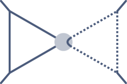
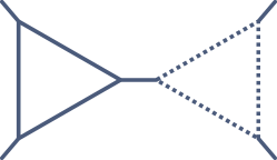
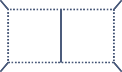
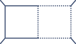
Figure 7: Representative Feynman diagrams contributing to $A_{1s}^{(2)}$. The grey circle symbolizes a quartic gluon–scalar vertex.

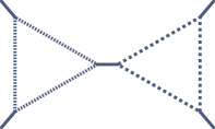
(a)

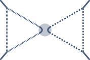
(b)

Figure 8: Representative of graphs contributing to $A_{D_{0},2,0}^{(2)}$ (a), and $A_{D_{0},1,1}^{(2)}$ (b). In (a), the scalar flavors in the two loops can be the same, while the quartic scalar interaction represented in (b) requires the flavors to be different. The quartic interaction with all scalars having the same flavor vanishes. After summing over scalar flavors the diagrams in (a) and (b) therefore appear with prefactors of $(D_{2}-D_{0})^{2}$ and $(D_{2}-D_{0})(D_{2}-D_{0}-1)$ respectively.

Given the specific Feynman rules above and the choices for the different dimensions, we can now make the decomposition in eq. (23) explicit,

$$A_{1}^{(2)} =A_{0}^{(2)}+(D_{1}-D_{0})A_{1s}^{(2)}+(D_{1}-D_{0})^{2}A_{2s}^{(2)}$$ (25)

$$=A_{0}^{(2)}+A_{1s}^{(2)}+A_{2s}^{(2)}\,,$$

$$A_{2}^{(2)} =A_{0}^{(2)}+(D_{2}-D_{0})A_{1s}^{(2)}+(D_{2}-D_{0})^{2}A_{2s}^{(2)}+(D_{2}-D_{0})(D_{2}-D_{0}-1)A_{\times}^{(2)}$$

$$=A_{0}^{(2)}+2A_{1s}^{(2)}+4A_{2s}^{(2)}+2A_{\times}^{(2)}\,.$$

When summing over the scalar-like degrees of freedom, each scalar loop in leads to a prefactor of $(D_{i}-D_{0})$ in the decomposition of $A_{i}^{(2)}$. In $A_{2}^{(2)}$, we find a contribution from the scalar contact term, which requires different scalars in the two loops. There are $(D_{2}-D_{0})(D_{2}-D_{0}-1)$ such combinations.

Substituting eq. (25) into eq. (22), we finally obtain

$$A_{D_{s}}^{(2)}=A_{0}^{(2)}+(D_{s}-D_{0})A_{1s}^{(2)}+(D_{s}-D_{0})^{2}A_{2s}^{(2)}+(D_{s}-D_{0})(D_{s}-D_{0}-1)A_{\times}^{(2)}.$$ (26)

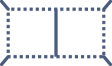
Figure 9: Diagrams with a single scalar loop contributing to the four-point amplitude.

Figure 10: Diagrams with a two scalar loops contributing to the four-point amplitude.

We can compare this result to similar approaches to two-loop computations in the literature. As an example, consider the BFZ derivation [11] of the four- and five-gluon all-plus amplitudes. BFZ obtained these amplitudes by decomposing the integrand,

$$\Delta_{D_{s}}^{(2)}=\Delta_{6}^{(2)}+(D_{s}-6)\Delta_{6,s}^{(2)}+(D_{s}-6)^{2}\Delta_{6,ss}^{(2)}\,,$$ (27)

where $\Delta_{6}^{(2)}$ is the full integrand of the six-dimensional amplitude, while $\Delta_{6,s}^{(2)}$ and $\Delta_{6,ss}^{(2)}$ are integrands from diagrams involving the extra-dimensional scalars. In the four-point amplitude, these scalar integrands correspond respectively to contributions from diagrams with a single scalar loop shown in Fig. 9 and diagrams with two distinct scalar loops shown in Fig. 10.

We must be careful in separating the contributions containing a four-scalar vertex, which necessarily have two scalar loops. We assign the contributions with identical scalars in loops to $\Delta_{6,s}^{(2)}$, while putting the contributions with different scalars in $\Delta_{6,ss}^{(2)}$.

For consistency between eq. (26) and eq. (27) with $D_{0}=6$ we need to have the correspondence [56],

$$\Delta_{6,s}^{(2)}\to\bigl{[}A_{1s}^{(2)}-A_{\times}^{(2)}\bigr{]}\big{|}_{D_{0}=6}\,,\quad\Delta_{6,ss}^{(2)}\to\bigl{[}A_{2s}^{(2)}+A_{\times}^{(2)}\bigr{]}\big{|}_{D_{0}=6}\,,$$ (28)

after integration. For $\Delta_{6,ss}^{(2)}$ we see that this is indeed the case, as the diagrams shown in Fig. 10 match the definitions of $A_{2s}^{(2)}$ and $A_{\times}^{(2)}$. For $\Delta_{6,s}^{(2)}$, we can obtain agreement using the relation,

$$A_{6,1,1}^{(2)}\simeq\includegraphics[height=28.45274pt,valign={c}]{dim_reconstruction/A2_11_1_picto}=-\includegraphics[height=28.45274pt,valign={c}]{dim_reconstruction/A2_11_single_scalar_1_picto}-\includegraphics[height=28.45274pt,valign={c}]{dim_reconstruction/A2_11_single_scalar_2_picto},$$ (29)

which follows from the quartic scalar Feynman rules of eq. (24).

Adding and subtracting terms to eq. (26), we can introduce an additional sampling dimension $D_{0}^{\prime}$, which may be smaller than four,

$$A_{D_{s}}^{(2)}= A_{0}^{(2)}+(D_{0}^{\prime}-D_{0})A_{1s}^{(2)}+(D_{0}^{\prime}-D_{0})^{2}A_{2s}^{(2)}+(D_{0}^{\prime}-D_{0})(D_{0}^{\prime}-D_{0}-1)A_{\times}^{(2)}$$ (30)

$$+(D_{s}-D_{0}^{\prime})\bigl{[}A_{1s}^{(2)}+2(D_{0}^{\prime}-D_{0})(A_{2s}^{(2)}+A_{\times}^{(2)})\bigr{]}$$

$$+(D_{s}-D_{0}^{\prime})^{2}A_{2s}^{(2)}+(D_{s}-D_{0}^{\prime})(D_{s}-D_{0}^{\prime}-1)A_{\times}^{(2)}.$$

II.3 Separability and Two-Loop Rational Terms

BMP showed [26] how to decompose the two-loop all-plus amplitudes into polylogarithmic terms $P_{n}^{(2)}$ and rational parts $R^{(2)}_{n}$ associated to different powers of the state dimension $D_{s}$. More precisely, through $\mathcal{O}(\epsilon^{0})$, BMP conjectured that these terms are associated to different powers of $D_{s}-2$,

$$F^{(2)}_{n:1}(1^{+}\mathellipsis n^{+})={\textstyle\frac{\textrm{\small 1}}{\lower 2.0pt\hbox{{\small 2}}}}(D_{s}-2)P^{(2)}(1^{+}\mathellipsis n^{+})+{\textstyle\frac{\textrm{\small 1}}{\lower 2.0pt\hbox{{\small 4}}}}(D_{s}-2)^{2}R^{(2)}(1^{+}\mathellipsis n^{+})+\mathcal{O}(\epsilon)\,.$$ (31)

BMP verified this decomposition for the five- and six-gluon leading color partial amplitudes by integrating the terms in the two-loop integrands proportional to $(D_{s}-2)^{2}$. They then checked the resulting analytic expressions numerically against the known results of refs. [32].

Let us now connect the BMP decomposition to the dimensional reconstruction picture explained in the previous subsection. Choose the base-dimension $D_{0}=6$, and use the rearrangement of eq. (30) with $D_{0}^{\prime}=2$. We then find,

$$P^{(2)} =2\bigl{[}P_{1s}^{(2)}-2\times 4\,(P_{2s}^{(2)}+P_{\times}^{(2)})-P_{\times}^{(2)}\bigr{]}\,,$$ (32)

$${R}^{(2)} =4\bigl{[}R_{2s}^{(2)}+R_{\times}^{(2)}\bigr{]}\,,$$

where $P_{1s}$, $P_{2s}$ and $P_{\times}$ are the finite polylogarithmic pieces of $A_{1s}$, $A_{2s}$ and $A_{\times}$, while $R_{2s}$, $R_{\times}$ are the corresponding rational parts. As we will often consider the sum of $R_{2s}$ and $R_{\times}$ for the rational parts of the all-plus, we will also use the shorthand,

$${R}^{(2)}_{ss}=R_{2s}+R_{\times}\,,$$ (33)

following ref. [11] and eq. (28).

Rephrasing the problem of computing $R$ in terms of $R_{2s}^{(2)}$ and $R_{\times}^{(2)}$ reduces its computational complexity. For $A_{2s}^{(2)}$, the two loops are connected through the exchange of a single gluon carrying no loop momentum; in $A_{\times}^{(2)}$, the two scalar lines of the two loops meet directly, but only in a four-scalar contact term. In neither case do both loop momenta appear in a single propogator, so that all required two-loop integrals factorize into a product of one-loop integrals. Because of the manner of simplification, we call the BMP conjecture the separability conjecture.

We can pick a basis of integrals which factorize as well. To determine the coefficients of these integrals in $A_{2s}^{(2)}$ and $A_{\times}^{(2)}$ using generalized unitarity cuts in each loop. We treat the loops sequentially. The first loop is computed from tree amplitudes using the standard one-loop unitarity technique; the second loop is computed from tree amplitudes and the coefficient computed at the first step, with the latter playing the role of a tree amplitude. In the second step, we again use the one-loop unitarity technique. We can pick either order for the two loops. The coefficient of the required two-loop integral is then the result of this two-stage computation.

Figure 11: A generic two-loop cut needed for $A_{2s}^{(2)}$ or $A_{\times}^{(2)}$. The two loops are connected only by a central tree amplitude, which contains no propagator dependent on both loop momenta. As we will see later, the shown attachment of the external gluons is associated to the leading-color trace structure $N_{c}^{2}\operatorname{Tr}$.

BMP made the separability conjecture for the leading-color partial amplitudes [26]. We extend the conjecture to rational contributions in subleading-color all-plus partial amplitudes as well, more specifically to those in nonplanar partial amplitudes. In later sections, we will discuss the construction of the non-planar versions of $A_{2s}^{(2)}$ and $A_{\times}^{(2)}$ via color-dressed unitarity, similar to the procedure for polylogarithmic contributions of refs. [34, 33]. We provide evidence for this extended conjecture through comparison of direct unitary-based computations of $A_{2s}^{(2)}$ and $A_{\times}^{(2)}$ for several subleading-color amplitudes to results in the literature [34]. These comparisons suggest that eq. (32) does indeed hold for all partial amplitudes in the color decomposition of two-loop all-plus amplitudes.

II.4 $D$-Dimensional Generalized Unitarity

The dimensional reconstruction procedure described earlier makes use of various integer dimensions for state-counting and matching in numerators of integrands. For the full integrands and for integrals, we of course must consider general dimensions $D=4-2\epsilon$ for the loop momenta.

As usual in modern applications of dimensional regularization, we take the external momenta to be strictly four-dimensional. We split the loop momenta into their four- and extra-dimensional components. The former we have already labeled $\bar{\ell}$; the latter we label $\breve{\ell}$,

$$\ell_{i}=\bar{\ell}_{i}+\breve{\ell}_{i}\,.$$ (34)

Because the external kinematics is four-dimensional, the $\breve{\ell}_{i}$ are conserved within each loop, and they can only appear in the Lorentz invariants,

$$\mu_{i}^{2}\equiv-(\breve{\ell}_{i}\cdot\breve{\ell}_{i})\,,\qquad\mu_{12}\equiv-(\breve{\ell}_{1}\cdot\breve{\ell}_{2})\,.$$ (35)

Separability ensures that the second invariant can only appear in the numerator; and in the numerator, performing either loop integral will make odd powers of it vanish, and will replace even powers with the result of integrating over powers of $\mu_{1}^{2}\mu_{2}^{2}$.

At this point we can follow the standard approach [30] for using one-loop $D$-dimensional generalized unitarity to compute rational terms. We separate the loop integrals into four- and extra-dimensional integrals,

$$\int\frac{d^{D}\ell}{(2\pi)^{D}}=\int\frac{d^{-\epsilon}\mu^{2}}{(2\pi)^{-2\epsilon}}\,\int\frac{\mathop{}\!\mathrm{d}^{4}\bar{\ell}}{(2\pi)^{4}}\,.$$ (36)

In cutting $D$-dimensional propagators, the massless on-shell condition for $\ell_{i}$ is then equivalent to a massive on-shell condition for $\bar{\ell}_{i}$,

$$\ell_{i}^{2}=0\ \Rightarrow\ \bar{\ell}_{i}^{2}=\mu_{i}^{2}\,,$$ (37)

where the latter can be thought of as constant for the inner integral. It corresponds to the scalar mass in the dimensional reconstruction approach discussed earlier. Were we to proceed and use generalized unitarity to obtain coefficients with respect to the inner integration, we would obtain expressions with rational dependence on the external spinor variables, and polynomial dependence on the $\mu_{i}^{2}$. Terms independent of $\mu_{i}^{2}$ correspond to four-dimensional cuts, and will lead to coefficients of the usual integrals. Terms with nontrivial powers of $\mu_{i}^{2}$ contain extra suppression, and will lead to either purely rational terms, or to terms of $\mathcal{O}(\epsilon)$. The maximal power of $\mu_{i}^{2}$ is limited by power counting: for boxes in Yang–Mills theories we get at most $\mu_{i}^{4}$, while for triangles and bubbles, at most $\mu_{i}^{2}$ is allowed. The box $\mu_{i}^{2}$ integral is of $\mathcal{O}(\epsilon)$, and therefore does not contribute.

A generic one-loop amplitude may therefore be written as follows [30],

$$A^{(1)} =\sum_{\textrm{boxes}}\operatorname{\mathrm{C}}^{(1)}_{{\mathrm{Box}},[0]}I^{D}_{4}[1]+\sum_{\textrm{triangles}}\operatorname{\mathrm{C}}^{(1)}_{{\mathrm{Tri}},[0]}I_{3}[1]+\sum_{\textrm{bubbles}}\operatorname{\mathrm{C}}^{(1)}_{{\mathrm{Bub}},[0]}I_{2}[1]$$ (38)

$$+\sum_{\textrm{boxes}}\operatorname{\mathrm{C}}^{(1)}_{{\mathrm{Box}},[4]}I^{D}_{4}[\mu^{4}]+\sum_{\textrm{triangles}}\operatorname{\mathrm{C}}^{(1)}_{{\mathrm{Tri}},[2]}I_{3}[\mu^{2}]+\sum_{\textrm{bubbles}}\operatorname{\mathrm{C}}^{(1)}_{{\mathrm{Bub}},[2]}I^{D}_{2}[\mu^{2}]+\mathcal{O}(\epsilon)\,,$$

where $I^{D}_{n}[\mathcal{N}]$ denotes an $n$-point $D$-dimensional integral with $\mathcal{N}$ inserted in its numerator. The coefficients $C_{\textrm{X},[j]}^{(1)}$ (corresponding to the $j^{\textrm{th}}$ power of $\mu$ in integral X), are rational functions of the external spinors. The integrals on the first line, without powers of $\mu^{2}$, can be obtained using four-dimensional generalized unitarity. They correspond to the parts of the amplitude that have branch cuts; in the case of the two-loop all-plus amplitude, these terms are known from refs. [13, 20, 19, 21, 15, 25, 24, 33]. The integrals on the second line of eq. (38) give rise to the rational parts of the amplitudes, using their values [30],

$$I^{D}_{4}[\mu^{4}] =-\frac{1}{6}+\mathcal{O}(\epsilon)\,,$$ (39)

$$I^{D}_{3}[\mu^{2}] =-\frac{1}{2}+\mathcal{O}(\epsilon)\,,$$

$$I^{D}_{2}[\mu^{2}] =-\frac{s}{6}+\mathcal{O}(\epsilon)\,.$$

Here, $s$ is the square of the momentum flowing through the bubble. The coefficients are given in terms of tree amplitudes,

$$\operatorname{\mathrm{C}}^{(1)}_{{\mathrm{Box}}} \equiv\operatorname{\mathrm{C}}^{(1)}_{{\mathrm{Box}},[4]}\equiv\operatorname{\mathrm{C}}^{(1)}_{{\mathrm{Box}},[4]}(A^{(0)}_{1},A^{(0)}_{2},A^{(0)}_{3},A^{(0)}_{4})\,,$$ (40)

$$\operatorname{\mathrm{C}}^{(1)}_{{\mathrm{Tri}}} \equiv\operatorname{\mathrm{C}}^{(1)}_{{\mathrm{Tri}},[2]}\equiv\operatorname{\mathrm{C}}^{(1)}_{{\mathrm{Tri}},[2]}(A^{(0)}_{1},A^{(0)}_{2},A^{(0)}_{3})\,,$$

$$\operatorname{\mathrm{C}}^{(1)}_{{\mathrm{Bub}}} \equiv\operatorname{\mathrm{C}}^{(1)}_{{\mathrm{Bub}},[2]}\equiv\operatorname{\mathrm{C}}^{(1)}_{{\mathrm{Bub}},[4]}(A^{(0)}_{1},A^{(0)}_{2})\,,$$

where the tree-amplitude arguments are understood to be functions of the parametrizations required to extract appropriate terms. In order to simplify the notation, we shall omit the subscript for the power of $\mu$ in coefficients contributing to the rational term.

The one-loop rational terms then have the form,

$${R}^{(1)}=-\frac{1}{6}\sum_{\textrm{boxes}}\operatorname{\mathrm{C}}^{(1)}_{{\mathrm{Box}}}-\frac{1}{2}\sum_{\textrm{triangles}}\operatorname{\mathrm{C}}^{(1)}_{{\mathrm{Tri}}}-\frac{1}{6}\sum_{\textrm{bubbles}}\operatorname{\mathrm{C}}^{(1)}_{{\mathrm{Bub}}}s^{\vphantom{(1)}}_{\textrm{Bub}}+\mathcal{O}(\epsilon)\,.$$ (41)

In the two-loop amplitudes $A^{(2)}_{2s}$ and $A^{(2)}_{\times}$, separability allows us to treat the loops consecutively. Their integral bases include all two-loop integrals which factorize into a product of one-loop integrals. We call such two-loop integrals “one-loop squared”.

As box, triangle and bubble integrals form a basis at one-loop, a basis of one-loop squared integrals is given by their unique products. There are six unique classes of such integrals,

$$I^{(2),D}_{{\textrm{Box},\textrm{Box}}} =\ I^{(1),D}_{4}[\mu^{4}]\times I^{(1),D}_{4}[\mu^{4}]\quad\sim\quad\includegraphics[valign={c},height=15.00002pt]{separability/intClasses/graph_1},$$ (42)

$$I^{(2),D}_{{\textrm{Box},\textrm{Tri}}} =\ I^{(1),D}_{4}[\mu^{4}]\times I^{(1),D}_{3}[\mu^{2}]\quad\sim\quad\includegraphics[valign={c},height=15.00002pt]{separability/intClasses/graph_2},$$

$$I^{(2),D}_{{\textrm{Box},\textrm{Bub}}} =\ I^{(1),D}_{4}[\mu^{4}]\times I^{(1),D}_{2}[\mu^{2}]\quad\sim\quad\includegraphics[valign={c},height=15.00002pt]{separability/intClasses/graph_3},$$

$$I^{(2),D}_{{\textrm{Tri},\textrm{Tri}}} =\ I^{(1),D}_{3}[\mu^{2}]\times I^{(1),D}_{3}[\mu^{2}]\quad\sim\quad\includegraphics[valign={c},height=15.00002pt]{separability/intClasses/graph_4},$$

$$I^{(2),D}_{{\textrm{Tri},\textrm{Bub}}} =\ I^{(1),D}_{3}[\mu^{2}]\times I^{(1),D}_{2}[\mu^{2}]\quad\sim\quad\includegraphics[valign={c},height=15.00002pt]{separability/intClasses/graph_5},$$

$$I^{(2),D}_{{\textrm{Bub},\textrm{Bub}}} =\ I^{(1),D}_{2}[\mu^{2}]\times I^{(1),D}_{2}[\mu^{2}]\quad\sim\quad\includegraphics[valign={c},height=15.00002pt]{separability/intClasses/graph_6},$$

As we are only interested in the rational parts ${R}^{(2)}_{2s}$ and ${R}^{(2)}_{\times}$, we take these integrals to always include $\mu^{2}$ or $\mu^{4}$ numerators for both loops. We will sometimes refer to $I^{(2),D}_{{\textrm{Tri},\textrm{Tri}}}$ and $I^{(2),D}_{{\textrm{Bub},\textrm{Bub}}}$ as ‘bow-tie’ and ‘spectacles’ integrals. In a complete basis of one-loop squared integrals we include integrals in these classes for all unique arrangements of the external momenta.

Each unique one-loop squared integral is accompanied by a coefficient. As for the integrals, there are six unique classes of such coefficients, which we label $\operatorname{\mathrm{C}}^{(2)}_{{\textrm{Box},\textrm{Box}}}$, $\operatorname{\mathrm{C}}^{(2)}_{{\textrm{Box},\textrm{Tri}}}$, $\operatorname{\mathrm{C}}^{(2)}_{{\textrm{Box},\textrm{Bub}}}$, $\operatorname{\mathrm{C}}^{(2)}_{{\textrm{Tri},\textrm{Tri}}}$, $\operatorname{\mathrm{C}}^{(2)}_{{\textrm{Tri},\textrm{Bub}}}$ and $\operatorname{\mathrm{C}}^{(2)}_{{\textrm{Bub},\textrm{Bub}}}$. As mentioned in the previous section, the coefficients can be determined by computing a one-loop coefficient with the other loop’s one-loop coefficient nested inside alongside tree amplitudes. As an example, in the one-loop unitarity language introduced above, the coefficient $\operatorname{\mathrm{C}}^{(2)}_{{\textrm{Tri},\textrm{Tri}}}$ of an integral $I_{{\textrm{Tri},\textrm{Tri}}}^{(2),D}$ would be computed as follows,

$$\operatorname{\mathrm{C}}^{(2)}_{\textrm{Tri},\textrm{Tri}}=\operatorname{\mathrm{C}}^{(1)}_{{\mathrm{Tri}},[2]}(A_{1}^{(0)},A_{2}^{(0)},\operatorname{\mathrm{C}}^{(1)}_{{\mathrm{Tri}},[2]}(A_{3}^{(0)},A_{4}^{(0)},A_{\textrm{C}}^{(0)}))\,.$$ (43)

Here, the amplitudes $A^{(0)}_{1,2}$ and $A^{(0)}_{3,4}$ are those of the two loops, which are themselves connected by $A^{(0)}_{\textrm{C}}$. Note that in the computation of the “outer” coefficient, the “inner” coefficient takes the role of an amplitude. As the two loops are equivalent, the choice of which loop’s coefficient to compute first is arbitrary. We could therefore just as well determine the same coefficient via

$$\operatorname{\mathrm{C}}^{(2)}_{\textrm{Tri},\textrm{Tri}}=\operatorname{\mathrm{C}}^{(1)}_{{\mathrm{Tri}},[2]}(A_{3}^{(0)},A_{4}^{(0)},\operatorname{\mathrm{C}}^{(1)}_{{\mathrm{Tri}},[2]}(A_{1}^{(0)},A_{2}^{(0)},A_{\textrm{C}}^{(0)}))\,.$$ (44)

To summarize, the rational parts ${R}^{(2)}_{2s}$ and ${R}^{(2)}_{\times}$ can be expressed as

$${R}^{(2)}_{2s,\times} =\frac{1}{36}\sum_{\textrm{box--boxes}}\operatorname{\mathrm{C}}^{(2)}_{\textrm{Box},\textrm{Box}}+\frac{1}{12}\sum_{\textrm{box--triangles}}\operatorname{\mathrm{C}}^{(2)}_{\textrm{Box},\textrm{Tri}}+\frac{1}{36}\sum_{\textrm{box--bubbles}}\operatorname{\mathrm{C}}^{(2)}_{\textrm{Box},\textrm{Bub}}s_{\textrm{Bub}}^{\vphantom{(1)}}$$ (45)

$$\hphantom{{}={}}+\frac{1}{4}\sum_{\textrm{triangle--triangles}}\operatorname{\mathrm{C}}^{(2)}_{\textrm{Tri},\textrm{Tri}}+\frac{1}{12}\sum_{\textrm{triangle--bubbles}}\operatorname{\mathrm{C}}^{(2)}_{\textrm{Tri},\textrm{Bub}}s_{\textrm{Bub}}^{\vphantom{(1)}}$$

$$\hphantom{{}={}}+\frac{1}{36}\sum_{\textrm{bubble--bubbles}}\operatorname{\mathrm{C}}^{(2)}_{\textrm{Bub},\textrm{Bub}}s_{\textrm{Bub}}^{\vphantom{(1)}}s_{\textrm{Bub}}^{\vphantom{(1)}}+\mathcal{O}(\epsilon)\,.$$

III Color Structure and Generating Sets of Cuts

We can write a complete two-loop $\text{SU}(N_{c})$ Yang–Mills amplitude as follows [34],

$$\mathcal{A}^{(2)}_{n} =N_{c}^{2}\sum_{\sigma\in{S_{n}}/{Z_{n}}}\mathop{\rm ITr}\nolimits\bigl{(}\sigma(1\mathellipsis n)\bigr{)}\,A^{(2)}_{n:1}\bigl{(}\sigma(1\mathellipsis n)\bigr{)}$$ (46)

$$+N_{c}\sum_{r=3}^{\lfloor{n}/{2}\rfloor+1}\sum_{\sigma\in{S_{n}}/{P_{n:r}}}\mathop{\rm ITr}\nolimits\bigl{(}\sigma(1\mathellipsis(r-1))\bigr{)}\mathop{\rm ITr}\nolimits\bigl{(}\sigma(r\mathellipsis n)\bigr{)}$$

$$\hskip 90.00014pt\times A^{(2)}_{n:r}\bigl{(}\sigma(1\mathellipsis(r-1);r\mathellipsis n)\bigr{)}$$

$$+\sum_{r=2}^{\lfloor{n}/{2}\rfloor}\sum_{k=r}^{\lfloor{(n-r)}/{2}\rfloor}\sum_{\sigma\in{S_{n}}/{P_{n:r,k}}}\mathop{\rm ITr}\nolimits\bigl{(}\sigma(1\mathellipsis r)\bigr{)}\mathop{\rm ITr}\nolimits\bigl{(}\sigma((r+1)\mathellipsis(r+k))\bigr{)}$$

$$\hskip 110.00017pt\times\mathop{\rm ITr}\nolimits\bigl{(}\sigma((r+k+1)\mathellipsis n)\bigr{)}$$

$$\hskip 90.00014pt\times A^{(2)}_{n:r,k}\bigl{(}\sigma(1\mathellipsis r;(r+1)\mathellipsis(r+k);(r+k+1)\mathellipsis n)\bigr{)}$$

$$+\sum_{\sigma\in{S_{n}}/{Z_{n}}}\mathop{\rm ITr}\nolimits\bigl{(}\sigma(1\mathellipsis n)\bigr{)}A^{(2)}_{n:1\mathrm{B}}\bigl{(}\sigma(1\mathellipsis n)\bigr{)}\,,$$

where the traces are,

$$\mathop{\rm ITr}\nolimits(i_{1}\mathellipsis i_{n})=\operatorname{Tr}(T^{a_{i_{1}}}\mathellipsis T^{a_{i_{n}}})\,.$$ (47)

For the double- and triple-trace color-ordered amplitudes, the sums over $r$ and $k$ are chosen such that the traces are ordered in increasing length. By $S_{n}$ and $Z_{n}$ we denote as usual the symmetric and cyclic groups on $n$ objects respectively. The permutation sets appearing above are,

$$P_{n:r} =\begin{cases}Z_{r-1}\times Z_{r-1}\times S_{2},&n=2(r-1)\,,\\ Z_{r-1}\times Z_{n-r-1},&\text{otherwise}\,;\end{cases},$$ (48)

$$P_{n:r,k} =\begin{cases}Z_{r}\times Z_{r}\times Z_{r}\times S_{3},&r=k,n=3r\,,\\ Z_{r}\times Z_{k}\times Z_{k}\times S_{2},&n=r+2k\,,\\ Z_{r}\times Z_{r}\times Z_{n-2r}\times S_{2},&r=k\,,\\ Z_{r}\times Z_{k}\times Z_{n-r-k},&\text{otherwise}\,.\end{cases}$$

These permutation sets account for the cyclic symmetry of the traces ($C_{i}$), as well as the exchanges of equal-length traces ($S_{i}$). The factors of $N_{c}$ in the decomposition may be interpreted as traces containing the identity $\mathbbm{1}_{N_{c}}$.

Our first task is to identify the two-loop cut topologies that contribute to the different trace structures in full-color all-plus amplitudes. It is useful to consider the corresponding string-theory amplitude, and use its color structure there as a guide for those in Yang–Mills theory [36]. This analysis was carried out at two loops in ref. [33].

Two-loop amplitudes in gauge theory can be obtained from taking the infinite-tension limit of the corresponding amplitudes in open string theory. The latter amplitudes are given as integrals over orientable world sheets of genus two with at least one boundary. There are two such surfaces: the disc with two punctures, which has three boundaries, and the punctured torus, which has only a single boundary. We show representations of these two surfaces in Figs. 12 and 13.

Figure 12: The Yang–Mills partial amplitudes $A^{{(2)}}_{n:1}$, $A^{{(2)}}_{n:r}$ and $A^{{(2)}}_{n:r,k}$ are associated to one-, two-, and three-trace color structures also present in three-boundary orientable genus-two surfaces in open string theory depicted here.

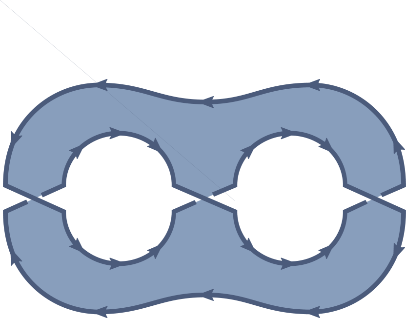
(a)

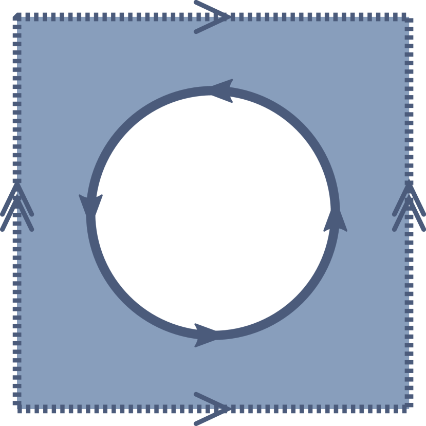
(b)

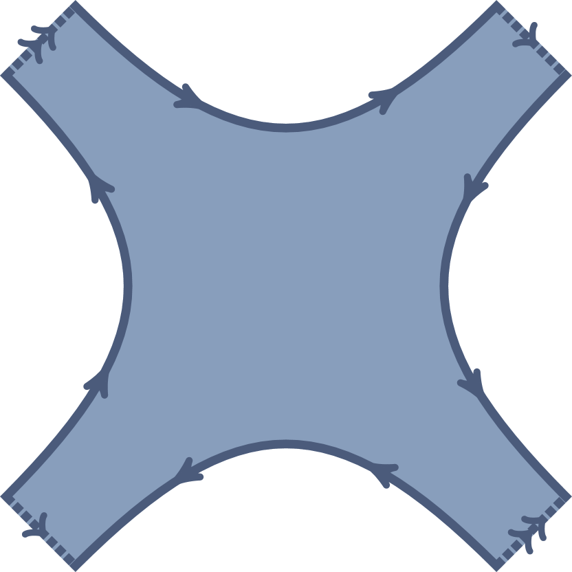
(c)

Figure 13: The Yang–Mills partial amplitudes $A^{(2)}_{n:1\mathrm{B}}$ are associated to single-trace color structures with no accompanying factors of $N_{c}$. These structures are also present in contributions to open-string amplitudes arising from orientable single-boundary genus-two surfaces. Three equivalent representations are shown: (a) as obtained from the doubly punctured disk of Fig. 12 (b) as equivalent to a punctured torus (c) the most useful representation for constructing the required unitarity cuts for the rational contributions to $A^{(2)}_{n:1\text{B}}$. In (b) and (c) the dotted lines must be sewn together with orientation given by their arrows.

Open strings are dressed with color factors $T^{a}_{ij}$ at their ends. Such factors are also inserted along world-sheet boundaries by the vertex operators coupling external states. The color-factor indices are contracted along each boundary, giving rise to color or Chan–Paton [58] factors, one trace per boundary. Traces with no vertex-operator insertion give rise to factors of $N_{c}$.

World sheets with the topology of Fig. 12 thus give rise to the color structures $N_{c}^{2}\operatorname{Tr}$, $N_{c}\operatorname{Tr}\operatorname{Tr}$, and $\operatorname{Tr}\operatorname{Tr}\operatorname{Tr}$, while world sheets with the topology of Fig. 13 give rise to single-trace structures with no accompanying factors of $N_{c}$. These are exactly the color structures we expect in Yang–Mills theories, and present in eq. (46).

We can reverse the sewing implicit in the Chan–Paton factors to obtain the sets of cuts needed for the full color-dressed amplitude, and thence the color-ordered cuts needed for each of the partial amplitudes. For example, consider the contributions from the cut shown in Fig. 14. All tree amplitudes appearing in the cut are color-ordered. Dressing the tree amplitudes with the color factors imposed by the cyclic ordering of their legs, the entire cut is associated to the color structure,

$$\mathop{\rm ITr}\nolimits(1,a,8,f)\mathop{\rm ITr}\nolimits(a,2,b,7)\mathop{\rm ITr}\nolimits(b,3,c,12,e,6,f)\mathop{\rm ITr}\nolimits(c,4,d,11)\operatorname{Tr}(d,5,e,10)\,.$$ (49)

Here, the indices $a,\ldots,f$ are implicitly summed over, as they are sewn across cuts. Using $U(N_{c})$ Fierz identities, we can carry out this sewing, ending up with a product of three traces,

$$\mathop{\rm ITr}\nolimits(1,2,3,4,5,6)\mathop{\rm ITr}\nolimits(7,8,9)\mathop{\rm ITr}\nolimits(10,11,12)\,.$$ (50)

recovering the three color traces we expected from Fig. 12. Color flows clockwise in the outer trace, and counter-clockwise in the two inner traces.

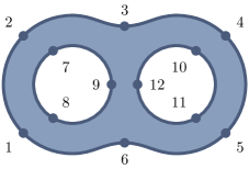
(a)

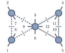
(b)

Figure 14: An example of a one-loop-squared cut contributing to the $A_{12;6,9}$ partial amplitude. As explained in the text, it contributions to the coefficient of the triple-trace structure $\mathop{\rm ITr}\nolimits(1,2,3,4,5,6)\mathop{\rm ITr}\nolimits(7,8,9)\mathop{\rm ITr}\nolimits(10,11,12)$.

The partial amplitudes $A_{n:1\mathrm{B}}^{(2)}$, on the other hand, arise from configurations which follow the structure of the punctured-torus worldsheet shown in Fig. 13. Fig. 13(a) shows the relation of this world-sheet to the doubly punctured disk, while Fig. 13(b) shows that this surface is indeed equivalent to a punctured torus. Finally, the representation of Fig. 13(c) is the one we will use to build color-ordered cuts. The corresponding sewing of tree amplitudes is illustrated at the one-loop squared cut shown in Fig. 15. The dotted lines at opposite corners are connected, similar to the orientation-preserving sewing of segments in Fig. 13(c).

The main difference in one-loop squared cuts originating from the doubly-punctured disk and punctured torus topologies lies in the connection of the scalar lines at the central vertex. In the former case, the two scalar lines are separated, while in the the latter they are required to cross. It is this crossing that produces the expected single trace color structure. We can verify this fact by carrying out the color algebra explicitly. For the particular cut shown in Fig. 15 we obtain,

$$\hphantom{={}}\mathop{\rm ITr}\nolimits(1,a,8,f)\mathop{\rm ITr}\nolimits(a,2,b,7)\mathop{\rm ITr}\nolimits(6,b,3,c,12,f,9,e)\mathop{\rm ITr}\nolimits(c,4,d,11)\mathop{\rm ITr}\nolimits(d,5,e,10)$$ (51)

$$=\mathop{\rm ITr}\nolimits(1,2,3,4,5,6,7,8,9,10,11,12)\,,$$

as promised.

(a)

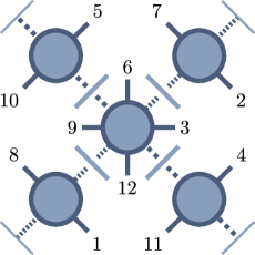
(b)

Figure 15: A graphical representation showing the heuristic relation between the string world-sheet and unitarity cuts of subleading single-trace amplitudes. The shown configuration belong to the color structure $\mathop{\rm ITr}\nolimits(1,2,\ldots,11,12)$. In both cases, the dotted lines need to be sewn together according to the arrows shown.

III.1 Leading-Color Partial Amplitudes

Let us now describe the required sets of cuts. We begin with the leading-color amplitude. A generic cut of this amplitude is shown in Fig. 16.

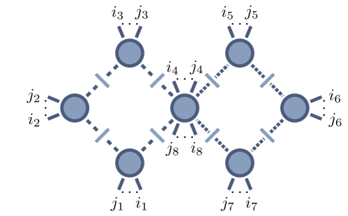
Figure 16: A generic cut for the leading-color rational part ${R}^{(2)}_{n:1}$

It sews a product of tree amplitudes along the left and right loops, joined by a four-scalar central amplitude. For the latter, we must include both gluon-exchange and four-scalar contact contributions.

To list all cuts systematically, we introduce labels for them. The label of a leading-color cut consists of four sets of sequences,

$$(E_{\textrm{L}};E_{\textrm{T}};E_{\textrm{R}};E_{\textrm{B}})\,.$$ (52)

The four sets correspond, in order, to amplitudes on the left loop ($E_{\textrm{L}}$); legs attached to the ‘top’ of the central amplitude ($E_{\textrm{T}}$); amplitudes on the right loop ($E_{\textrm{R}}$); and legs attached to the ‘bottom’ of the central amplitude ($E_{\textrm{B}}$). Each of these sets contains a number of sequences, which list the external legs attached to a tree amplitude. As the left and right loop are made up of either bubbles, triangles or boxes, the sets $E_{\textrm{L}}$ and $E_{\textrm{R}}$ have either one, two or three of these sequences,

$$E_{\textrm{L}}=\left\{\begin{aligned} &{(i_{1}\ldots j_{1})}\,,\\ &{(i_{1}\ldots j_{1}),(i_{2}\ldots j_{2})}\,,\\ &{(i_{1}\ldots j_{1}),(i_{2}\ldots j_{2}),(i_{3}\ldots j_{3})}\,,\end{aligned}\right.$$ (53)

along with a similar form for $E_{\textrm{R}}$. The sets $E_{\textrm{T}}$ and $E_{\textrm{B}}$ only contain a single sequence,

$$E_{{\textrm{T}},{\textrm{B}}} ={(i\ldots j)}\,,$$ (54)

In each sequence, the external leg labels are shown according to their clockwise order around the outside of the diagram. As an example, the cut of the $n$-point leading-color partial amplitude shown in Fig. 16 carries the label,

$$({(i_{1},\ldots,j_{1}),(i_{2},\ldots,j_{2}),(i_{3},\ldots,j_{3})};{(i_{4},\ldots,j_{4})};\\ {(i_{5},\ldots,j_{5}),(i_{6},\ldots,j_{6}),(i_{7},\ldots,j_{7})};{(i_{8},\ldots,j_{8})}).$$ (55)

Any such label corresponds to a unitarity cut, provided that it satisfies two conditions:

1. When $E_{\textrm{L}}$ or $E_{\textrm{R}}$ contain only a single sequence (i.e. the corresponding loop is a bubble), this sequence has to contain at least two elements, to avoid scaleless bubbles.

2. When $E_{\textrm{L}}$ or $E_{\textrm{R}}$ contain two or three sequences (corresponding to a triangle or a box), each sequence needs to contain at least one element. In other words, all tree amplitudes are at least three-point amplitudes.

We call the set of all labels eq. (55) for $n$ momenta that satisfy these conditions $\mathrm{AllLabels}_{n:1}.$

In order to compute the rational contribution to the leading-color partial amplitude $R^{(2)}_{n:1}(1,\ldots,n)$, we need to sum over all unique cuts. However, a cut does not have a single unique label. We still have to account for the equivalence of the two loops, giving each cut a $\mathbb{Z}_{2}$ symmetry. This symmetry manifests itself in the cuts through an equivalence relation $\operatorname{Exch}$, whose action is given by,

$$\operatorname{Exch}\bigl{[}(E_{\textrm{L}};E_{\textrm{T}};E_{\textrm{R}};E_{\textrm{B}})\bigr{]}=(E_{\textrm{R}};E_{\textrm{B}};E_{\textrm{L}};E_{\textrm{T}})\,.$$ (56)

This can be thought of as rotating a cut diagram by 180^∘ in the plane.

We associate each label to one of the six integral classes of shown in eq. (42). For each such class $C$, we define $\mathrm{AllLabels}_{n:1}(C)$ to be the set of all cut labels belonging to that class. Due to the equivalence of the loops, there are always two labels associated to a unitarity cut. For example, the labels

$$((1),(2),(3);();(4),(5);()),\quad((4),(5);();(1),(2),(3);())$$ (57)

are both elements of $\mathrm{AllLabels}({\{{\textrm{Box},\textrm{Tri}}\}})$, while describing the same cut, as they are related by $\operatorname{Exch}$. We therefore introduce the set $\mathrm{UniqueCuts}_{n:1}$, which contains one label per unique cut. As $\operatorname{Exch}$ only relates labels of the same class, we can construct $\mathrm{UniqueCuts}_{n:1}$ in terms of equivalence classes of $\mathrm{AllLabels}_{n:1}(C)$,

$$\mathrm{UniqueCuts}_{n:1}=\bigcup\limits_{\text{classes }C}\left(\raisebox{3.0pt}{$\mathrm{AllLabels}_{n:1}(C)$}\bigg{/}\raisebox{-3.0pt}{$\operatorname{Exch}$}\right)\,.$$ (58)

For the rational part of the leading-color partial amplitude we then sum over the contributions associated to the labels in $\mathrm{UniqueCuts}_{n:1}$,

$${R}^{(2)}_{n:1}(1,\ldots,n)=\sum_{c\in\mathrm{UniqueCuts}_{n:1}}{R}^{(2)}_{c}(1,\ldots,n).$$ (59)

Each index $c$ can be given in the form described in eq. (52), with ${R}^{(2)}_{c}$ the rational contribution from that cut. We give the precise definition of ${R}^{(2)}_{c}$ in section III.4.

We can go one step further and make the cyclic symmetry of the all-plus configuration manifest. We define $\tilde{{R}}^{(2)}$ through the property that,

$$R^{(2)}_{n:1}(1,\ldots,n)=\sum_{\rho\in Z_{n}}\tilde{{R}}^{(2)}(\rho[1,\ldots,n])\,.$$ (60)

To determine such an $\tilde{{R}}^{(2)}$ we require only a generating subset of all unitarity cuts $G_{n:1}\subset\mathrm{UniqueCuts}_{n:1}$. We obtain such a subset by identifying cut labels that are related by a cyclic permutation of the external particles,

$$G_{n:1}=\left(\raisebox{3.0pt}{$\mathrm{UniqueCuts}_{n:1}$}\bigg{/}\raisebox{-3.0pt}{$Z_{n}$}\right)=\bigcup\limits_{\text{classes }C}\left(\raisebox{3.0pt}{$\mathrm{AllLabels}_{n:1}(C)$}\bigg{/}\raisebox{-3.0pt}{$\operatorname{Exch}\times Z_{n}$}\right)\,.$$ (61)

We can realize the identification of cut labels under $Z_{n}$ by fixing the position of one of the momenta. We always make the choice that for each label in $G_{n:1}$ we have

$$E_{\textrm{L}}={(1,\mathellipsis),\mathellipsis}\,.$$ (62)

In the generic cut of Fig. 16 this corresponds to setting $i_{1}=1$. As a more concrete example, consider the following two labels belonging to cuts of ${R}^{(2)}_{5:1}$,

$$c=({(1),(2)};();{(3),(4)};(5)),\quad c^{\prime}=({(1),(2)};(3);{(4),(5)};())\,.$$ (63)

Their associated cuts are shown in Fig. 17(a).

(a) Example of a cut that is related to another cut via $Z_{5}\times\operatorname{Exch}$. We obtain the cut on the right from the one one the left by switching the two loops and cycling the external labels by two positions. We therefore include only one of these cuts in $G_{n:1}$.

(b) Example of a cut that is invariant under $Z_{6}\times\operatorname{Exch}$. Swapping the loops and cycling the external labels by three places leaves the cut invariant. We must therefore include this cut in $G_{n:1}$ and associate to it a symmetry factor of $\tfrac{1}{2}$.

Figure 17: Examples of relations between cuts for the leading-color rational parts ${R}^{(2)}_{n:1}$.

Of these two labels, we only include one in $G_{n:1}$, as,

$$\operatorname{Exch}\circ\,\rho_{2}\left[({(1),(2)};();{(3),(4)};(5))\right]$$ (64)

$$= \operatorname{Exch}[({(4),(5)};();{(1),(2)};(3))]$$

$$= ({(1),(2)};(3);{(4),(5)};())\,,$$

with $\rho_{2}\in Z_{5}$ representing the clockwise shift of all labels by two positions.

The generator function $\tilde{{R}}^{(2)}$ is determined by summing over all labels within $G_{n:1}$, accompanied by a symmetry factor $S^{\vphantom{(1)}}_{c}$,

$$\tilde{{R}}^{(2)}(1,\ldots,n)=\sum_{c\in G_{n:1}}S^{\vphantom{(1)}}_{c}\,\tilde{{R}}^{(2)}_{c}(1,\ldots,n)\,.$$ (65)

The symmetry factors are necessary to compensate for the overcounting of cuts that are invariant under the combined action of $\operatorname{Exch}$ and $Z_{n}$. An example would be the label

$$c=({(1,2),(3)};();{(4,5),(6)};())$$ (66)

of ${R}^{(2)}_{6:1}$. This cut label is invariant under shifting the momenta three places via $\rho_{3}\in Z_{6}$ and exchanging the loops,

$$\operatorname{Exch}\circ\,\rho_{3}\left[({(1,2),(3)};();{(4,5),(6)};())\right]$$ (67)

$$= \operatorname{Exch}[({(4,5),(6)};();{(1,2),(3)};())]$$

$$= ({(1,2),(3)};();{(4,5),(6)};())$$

This relation is shown diagrammatically in Fig. 17(b).

Such an invariance can only occur for cut labels of the classes ${\{{\textrm{Box},\textrm{Box}}\}}$, ${\{{\textrm{Tri},\textrm{Tri}}\}}$ and ${\{{\textrm{Bub},\textrm{Bub}}\}}$ with an even number of external particles. It causes the associated cut to appear twice in the sum over cyclic permutations, and therefore requires a symmetry factor of $S_{c}=\tfrac{1}{2}$. For all remaining cuts we have $S_{c}=1$.

At one loop, computing the bubble coefficient using the approach of refs.[29, 30] requires not only the bubble cut itself, but also computing three-propagator cuts from parent triangles. These must then be accounted for according to eq. (284).

In computing the coefficients of one-loop squared integrals we must of course also include such contributions. Specifically, for every cut-label in the generating set $G_{n:1}$ involving a bubble cut, we must also include cuts where the bubble cut is replaced with a triangle cut. Consider for example the cut shown in Fig. 18 belonging to a $G_{5:1}$. In addition to the two bubble cuts seen at the top, we also in general need to compute the seven additional parent-triangle cuts shown below it. Here the short-dashed lines represent the extra cut introduced in addition to the original bubble cut. In this procedure, only those cuts are allowed that belong to a one-loop squared topology. Any topologies with a propagator depending on both loop momenta are still forbidden by the scalar Feynman rules.

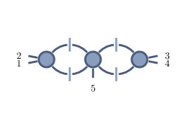
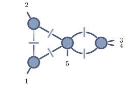
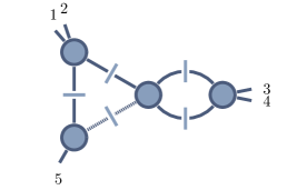
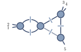
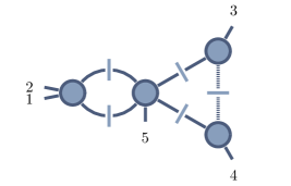
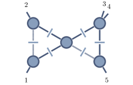
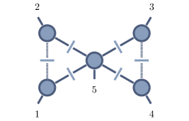
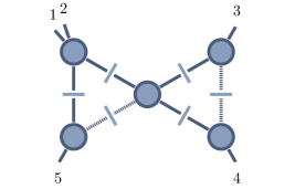
Figure 18: Examples of parent-triangle contributions that together with the bubble cut make up the bubble coefficient. For visual clarity, the cut propagators of the bubbles are shown as solid lines, while the additionally cut propagators are shown as dashed lines.

III.2 Two- and Three-Trace Partial Amplitudes

We turn next to the more general case of subleading-color double- and triple-trace partial amplitudes. In the following we focus on the coefficients of $\operatorname{Tr}(\cdots)\operatorname{Tr}(\cdots)\operatorname{Tr}(\cdots)$. The coefficients of $N_{c}\operatorname{Tr}(\cdots)\operatorname{Tr}(\cdots)$ can be obtained using the same strategy by leaving one of the traces empty.

A generic three-trace cut has the form shown in Fig. 19.

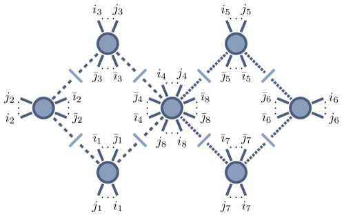
Figure 19: A generic cut for the sub-leading color rational part ${R}^{(2)}_{n:kl}$.

To attach labels to such cuts, we extend the notation of eq. (52) by two further sets, separated by vertical bars. From the point of view of Fig. 14, these sets describe the attachment of legs to the inner edges of the left and right loops. We denote them respectively by a subscript L or R on the vertical bar. For simplicity, let us first consider the case where external particles are only attached to the inside of the left loop. A corresponding cut label takes the form,

$$(E_{\textrm{L}};E_{\textrm{T}};E_{\textrm{R}};E_{\textrm{B}}|_{\textrm{L}}E_{\textrm{C},\textrm{L}};E_{\textrm{I},\textrm{L}})\,.$$ (68)

Here, $E_{\textrm{L},{\textrm{T}},\textrm{R},{\textrm{B}}}$ denote the legs on the ‘outside’ of the diagram, $E_{\textrm{C},\textrm{L}}$ is the sequence of legs attached to central amplitude ‘inside’ the (left) loop, while $E_{\textrm{I},\textrm{L}}$ collects the legs attached to the ‘inside’ of tree amplitudes along the (left) loop. As $E_{\textrm{L}}$ and $E_{\textrm{I},\textrm{L}}$ describe the attachments to the same amplitudes, just ’inside’ and ’outside’ of the loop, they need to have the same number of sequences—one for each amplitude in the loop. The legs within each sequence of $E_{\textrm{I},\textrm{L}}$ are attached to the same tree amplitude as those of the same-ordinal sequence with $E_{\textrm{L}}$. However, due to the reversed color-flow on the inside of the loop, they are attached in reverse order. That is, a label with,

$$E_{\textrm{L}} =(i_{1}\cdots j_{1})\cdots(i_{3}\cdots j_{3})\,,$$ (69)

$$E_{\textrm{I},\textrm{L}} =(\bar{\jmath}_{1}\cdots\bar{\imath}_{1})\cdots(\bar{\jmath}_{3}\cdots\bar{\imath}_{3})\,,$$

corresponds to a cut containing the tree amplitudes

$$A^{(0)}(i_{1},\ldots j_{1},-\ell_{1},\bar{\imath}_{1},\ldots,\bar{\jmath}_{1},\ell_{2})\times\cdots\times A^{(0)}(i_{3},\ldots j_{3},-\ell_{3},\bar{\imath}_{3},\ldots,\bar{\jmath}_{3},\ell_{4})\,,$$ (70)

attached to a color structure of the form

$$\mathop{\rm ITr}\nolimits(i_{1}\cdots j_{1}\cdots i_{3}\cdots j_{3}\cdots)\mathop{\rm ITr}\nolimits(\bar{\imath}_{3}\cdots\bar{\jmath}_{3}\cdots\bar{\imath}_{1}\cdots\bar{\jmath}_{1}\cdots)\cdots\,.$$ (71)

As particles can now also be attached to the inside of a loop, we need to extend the restrictions introduced for labels of leading-color labels, which guarantee massive bubbles and tree amplitudes being at least of three-point type. They are respectively:

1. If $E_{\textrm{L}}$ and $E_{\textrm{I},\textrm{L}}$ each contain only one sequence, they together need to contain at least two elements in total.

2. Sequences from $E_{\textrm{L}}$ and $E_{\textrm{I},\textrm{L}}$ belonging to the same amplitude have to contain at least one element in total.

As long as these conditions are satisfied, sequences may contain any number of elements. In particular, they may now also be empty.

The extension to general cuts with the three-trace color structure is now simple: when attaching external particles to the inner edges of both the left and right loop, we add two sets to a cut label,

$$(E_{\textrm{L}};E_{\textrm{T}};E_{\textrm{R}};E_{\textrm{B}}|_{\textrm{L}}E_{\textrm{C},\textrm{L}};E_{\textrm{I},\textrm{L}}|_{\textrm{R}}E_{\textrm{C},\textrm{R}};E_{\textrm{I},\textrm{R}})\,,$$ (72)

where the number of sequences in $E_{\textrm{I},\textrm{L}}$ ($E_{\textrm{I},\textrm{R}}$) must match that of $E_{\textrm{L}}$ ($E_{\textrm{R}}$). The conditions required by every amplitude having a particle attached and the vanishing of massless bubbles now need to be satisfied by both loops, i.e. for both pairs $E_{\textrm{L}}$,$E_{\textrm{I},\textrm{L}}$ and $E_{\textrm{R}}$,$E_{\textrm{I},\textrm{R}}$. The legs in $E_{\textrm{I},\textrm{R}}$ are now also given in reverse order compared to how they appear in the color-ordering, and just as in the left loop, the legs of sequences in $E_{\textrm{I},\textrm{R}}$ are attached to the same tree amplitude as those of the same-ordinal sequence of $E_{\textrm{R}}$. The generic cut shown in Fig. 19 for example carries the label

$$( {(i_{1},\ldots,j_{1}),(i_{2},\ldots,j_{2}),(i_{3},\ldots,j_{3})};{(i_{4},\ldots,j_{4})};$$ (73)

$${(i_{5},\ldots,j_{5}),(i_{6},\ldots,j_{6}),(i_{7},\ldots,j_{7})};{(i_{8},\ldots,j_{8})}$$

$$|_{\textrm{L}}(\bar{\jmath}_{4},\ldots,\bar{\imath}_{4});(\bar{\jmath}_{1},\ldots,\bar{\imath}_{1}),(\bar{\jmath}_{2},\ldots,\bar{\imath}_{2}),(\bar{\jmath}_{3},\ldots,\bar{\imath}_{3})$$

$$|_{\textrm{R}}(\bar{\jmath}_{8},\ldots,\bar{\imath}_{8});(\bar{\jmath}_{5},\ldots,\bar{\imath}_{5}),(\bar{\jmath}_{6},\ldots,\bar{\imath}_{6}),(\bar{\jmath}_{7},\ldots,\bar{\imath}_{7})).$$

As in the leading-color case, we have an equivalence relation $\operatorname{Exch}$, due to equivalence of the two scalar loops. Its action on the label of a two- or three-trace cut is given by,

$$\operatorname{Exch}\bigl{[}(E_{\textrm{L}};E_{\textrm{T}};E_{\textrm{R}};E_{\textrm{B}}|_{X}E_{\textrm{C},X};E_{\textrm{I},X})\bigr{]}=(E_{\textrm{R}};E_{\textrm{B}};E_{\textrm{L}};E_{\textrm{T}}|_{\operatorname{Exch}(X)}E_{\textrm{C},X};E_{\textrm{I},X})\,,$$ (74)

$$\operatorname{Exch}\bigl{[}(E_{\textrm{L}};E_{\textrm{T}};E_{\textrm{R}};E_{\textrm{B}}|_{\textrm{L}}E_{\textrm{C},\textrm{L}};E_{\textrm{I},\textrm{L}}|_{\textrm{R}}E_{\textrm{C},\textrm{R}};E_{\textrm{I},\textrm{R}})\bigr{]}=$$

$$\hskip 99.58464pt(E_{\textrm{R}};E_{\textrm{B}};E_{\textrm{L}};E_{\textrm{T}}|_{\textrm{L}};E_{\textrm{C},\textrm{R}}E_{\textrm{I},\textrm{R}}|_{\textrm{R}}E_{\textrm{C},\textrm{L}};E_{\textrm{I},\textrm{L}})\,,$$

where in the former case we can have $X\in\{L,R\}$, while $\operatorname{Exch}(\textrm{L})=\textrm{R}$ and $\operatorname{Exch}(\textrm{R})=\textrm{L}$.

We use the string picture as a guide to construct the required cuts as shown in Fig. 14. In the case of the string amplitude, the three boundaries of the world-sheet—and therefore the color traces—are on equal footing. We can smoothly deform the worldsheet, such that any two edges switch places. The form of the worldsheet shown in Fig. 20(a) makes this property manifest. However, when considering corresponding cuts as shown in Fig. 19, this symmetry between the different edges is no longer present. In particular, we cannot deform the cut, such that the particles on the ‘outside’ appear on the ‘inside’ of one of the loops; the ‘outer’ edge of the a cut is therefore distinct. The resolution of this discrepancy is that the symmetry is not present at the level of individual cuts. Rather, to restore it for the full amplitude we need sum over cuts for each permutation of the edges, as exemplified in Fig. 20(b).

(a) Representation of the world-sheet that makes the equivalence of the three edges evident.

(b) The six representations of the same world-sheet used to construct gauge-theory cuts.

Figure 20: An example of a two-puncture disk open-string world-sheet. Fig. (a) shows a three-dimensional embedding making the equivalence of the three edges manifest. Fig. (b) shows the six different representations, for which we construct unitarity cuts. The insertions on the edges correspond to a color structure $\mathop{\rm ITr}\nolimits(1,2,3)\mathop{\rm ITr}\nolimits(4,5,6)\mathop{\rm ITr}\nolimits(7,8,9)$

To be more explicit, let $\operatorname{Tr}_{1}$, $\operatorname{Tr}_{2}$ and $\operatorname{Tr}_{3}$ be the three color traces, and let $\sigma$ be a permutation of the set $\{\operatorname{Tr}_{1},\operatorname{Tr}_{2},\operatorname{Tr}_{3}\}$. Define $\mathrm{AllLabels}^{\sigma}\equiv\mathrm{AllLabels}^{\{\sigma(1),\sigma(2),\sigma(3)\}}$ to be the set of all cut labels of the form given in eq. (73), in which the traces $\sigma(1)$, $\sigma(2)$ and $\sigma(3)$ are associated to the outer, left inner and right inner edge. The momenta associated to $\sigma(1)$ therefore make up the sets $E_{\textrm{L}}$, $E_{\textrm{T}}$, $E_{\textrm{R}}$, $E_{\textrm{B}}$, while those of $\sigma(2)$ and $\sigma(3)$ respectively determine $E_{\textrm{I},\textrm{L}}$, $E_{\textrm{C},\textrm{L}}$ and $E_{\textrm{I},\textrm{R}}$, $E_{\textrm{C},\textrm{R}}$.

The set of all labels compatible with a triple trace color structure is then

$$\mathrm{AllLabels}_{n:kl}=\bigcup\limits_{\sigma\in S_{3}(\{\operatorname{Tr}_{1},\operatorname{Tr}_{2},\operatorname{Tr}_{3}\})}\mathrm{AllLabels}^{\sigma}$$ (75)

For the rational part ${R}^{(2)}_{n:kl}$ we again require only unique cuts. Just as in the leading-color case, $\mathrm{AllLabels}_{n:kl}$ contains two labels for each cut, related by $\operatorname{Exch}$. Consider for example, the labels

$$((1),();();(2),()|_{\textrm{L}}();(4),(3)|_{\textrm{R}}();(6),(5))\,,$$ (76)

$$((2),();();(1),()|_{\textrm{L}}();(6),(5)|_{\textrm{R}}();(4),(3))\,,$$

of ${R}^{(2)}_{6:2,2}$, whose visual representation is given in Fig. 21. For $\operatorname{Tr}_{1}=\mathop{\rm ITr}\nolimits(1,2)$, $\operatorname{Tr}_{2}=\mathop{\rm ITr}\nolimits(3,4)$, $\operatorname{Tr}_{3}=\mathop{\rm ITr}\nolimits(5,6)$, these labels belong respectively to $\mathrm{AllLabels}^{\{\operatorname{Tr}_{1},\operatorname{Tr}_{2},\operatorname{Tr}_{3}\}}$ and $\mathrm{AllLabels}^{\{\operatorname{Tr}_{1},\operatorname{Tr}_{3},\operatorname{Tr}_{2}\}}$. Both therefore appear in $\mathrm{AllLabels}_{6:2,2}$. However, from Fig. 21 it is easy to see that these labels describe the same unitarity cut.

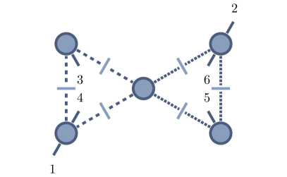
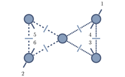
Figure 21: Graphic representation of two labels belonging to the same unitarity cut of ${R}^{(2)}_{6:2,2}$.

Accordingly we find that they are related by $\operatorname{Exch}$,

$$\hphantom{{}={}}\operatorname{Exch}\bigl{[}((1),();();(2),()|_{\textrm{L}}();(4),(3)|_{\textrm{R}}();(6),(5))\bigr{]}$$ (77)

$$=((2,();();(1),()|_{\textrm{L}}();(6),(5)|_{\textrm{R}}();(4),(3))$$

Modding out such relations, we obtain the set of unique cuts,

$$\mathrm{UniqueCuts}_{n:kl}=\raisebox{5.0pt}{$\Biggl{(}\,\mathrm{AllLabels}_{n:kl}\Biggr{)}$}\bigg{/}\raisebox{-3.0pt}{$\operatorname{Exch}$}\,.$$ (78)

We can give a more concise form of this set. As $\operatorname{Exch}$ switches the trace assignments of the inner edges, we find that,

$$\operatorname{Exch}\left[\mathrm{AllLabels}^{\{\operatorname{Tr}_{1},\operatorname{Tr}_{2},\operatorname{Tr}_{3}\}}\right]=\mathrm{AllLabels}^{\{\operatorname{Tr}_{1},\operatorname{Tr}_{3},\operatorname{Tr}_{2}\}}$$ (79)

It is therefore simple to realize the action of $\operatorname{Exch}$ in eq. (78): for every assignment of a trace to the outer edge, we include only one of the two possible left and right inner edge trace assignments. We therefore only sum over cyclic permutations of $\{\operatorname{Tr}_{1},\operatorname{Tr}_{2},\operatorname{Tr}_{3}\}$, so that

$$\mathrm{UniqueCuts}_{n:kl}=\bigcup_{\sigma\in Z_{3}(\{\operatorname{Tr}_{1},\operatorname{Tr}_{2},\operatorname{Tr}_{3}\})}\mathrm{AllLabels}^{\sigma},$$ (80)

The rational part for the color structure $\mathop{\rm ITr}\nolimits(1,\ldots,k)\mathop{\rm ITr}\nolimits(k+1,\ldots,k+l)\mathop{\rm ITr}\nolimits(k+l+1,\ldots,n)$ is then,

$${R}^{(2)}_{n:kl}(1,\ldots,k;k+1,\ldots,k+l;k+l+1,\ldots,n)\\ =\sum_{c\in\mathrm{UniqueCuts}_{n:kl}}{R}^{(2)}_{c}(1,\ldots,k;k+1,\ldots,k+l;k+l+1,\ldots,n).$$ (81)

As in the leading-color case we can make the cyclic symmetry of the partial amplitudes manifest. We define a function $\tilde{{R}}^{(2)}_{n:kl}$, which reproduces the full rational part after summing over cyclic permutations of particles in each trace,

$${R}^{(2)}_{n:kl}(1,\ldots,k;k+1,\ldots,k+l;k+l+1,\ldots,n)\\ =\sum_{\rho\in Z_{n:kl}}\tilde{{R}}^{(2)}_{n:kl}(\rho[1,\ldots,k;k+1,\ldots,k+l;k+l+1,\ldots,n]).$$ (82)

Here, $Z_{n:kl}=Z_{k}\times Z_{l}\times Z_{n-k-l}$ is the group of cyclic permutations of all three traces. We again obtain $\tilde{{R}}^{(2)}_{n:kl}$ from a generating set of cut labels $G_{n:kl}\subset\mathrm{UniqueCuts}_{n:kl}$, together with potential symmetry factors $S_{c}$, i.e.

$$\tilde{{R}}^{(2)}_{n:kl}(1,\ldots,k;k+1,\ldots,k+l;k+l+1,\ldots,n)\\ =\sum_{c\in G_{n:kl}}S_{c}{R}^{(2)}_{c}(1,\ldots,k;k+1,\ldots,k+l;k+l+1,\ldots,n).$$ (83)

We can again find such a generating set by identifying any unique cuts that are related by a cyclic permutation of the traces,

$$G_{n:kl}=\raisebox{3.0pt}{$\mathrm{AllLabels}_{n:kl}$}\bigg{/}\raisebox{-3.0pt}{$\operatorname{Exch}\times Z_{n:kl}$}=\bigcup_{\sigma\in Z_{3}(\{\operatorname{Tr}_{1},\operatorname{Tr}_{2},\operatorname{Tr}_{3}\})}\raisebox{3.0pt}{$\mathrm{AllLabels}^{\sigma}$}\bigg{/}\raisebox{-3.0pt}{$Z_{n:kl}$}.$$ (84)

To find an explicit form of $G_{n:kl}$, we fix for every edge the position of one particle. Given cut labels $\mathrm{AllLabels}^{\sigma}$ with

$$\sigma=\{\mathop{\rm ITr}\nolimits(1,\ldots,k),\mathop{\rm ITr}\nolimits(k+1,\ldots,k+l),\mathop{\rm ITr}\nolimits(k+l+1,\ldots,n)\}\}\,,$$ (85)

we choose to keep those labels in which the particles $1$, $k+1$ and $k+l+1$ are at the first position after the central vertex in the color-ordering. For each such label we have,

$$E_{\textrm{L}}\cup E_{{\textrm{T}}}\cup E_{\textrm{R}}\cup E_{{\textrm{B}}} =(1,\ldots),\ldots\,,$$ (86)

$$E_{\textrm{C},\textrm{L}}\cup E_{\textrm{I},\textrm{L}} =\ldots,(\ldots,k+1)\,,$$

$$E_{\textrm{C},\textrm{R}}\cup E_{\textrm{I},\textrm{R}} =\ldots,(\ldots,k+l+1)\,.$$

In the cut of Fig. 19 this corresponds to

$$i_{1}=1,\quad\bar{\imath}_{3}=k+1,\quad\bar{\imath}_{7}=k+l+1\,.$$ (87)

The sequence containing $1$ in $E_{\textrm{L}}\cup E_{{\textrm{T}}}\cup E_{\textrm{R}}\cup E_{{\textrm{B}}}$ can potentially be preceded by empty sequences. Similarly, the sequences containing $k+1$ and $k+l+1$ in $E_{\textrm{C},\textrm{L}}\cup E_{\textrm{I},\textrm{L}}$ and $E_{\textrm{C},\textrm{R}}\cup E_{\textrm{I},\textrm{R}}$ can be followed by empty sequences.

In contrast to the leading-color case, we do not require symmetry factors here, so that $S_{c}=1$ for all labels $c\in G_{n:kl}$. This absence of symmetry factors is due to the three traces being unique. At leading color, the symmetry factors were necessary due to an overcounting of cuts, where the associated labels are invariant under $\operatorname{Exch}$ and cyclic permutation of the external legs. From the point of view of the present discussion, this type of equivalence relies on the two traces assigned to the insides of the loops being identical—in the leading-color case they are both empty. If all traces are unique, such invariant labels do not exist, and there is no overcounting of cuts.

We again have to include for every bubble cut in $G_{n:kl}$ the corresponding set of parent triangle cuts, which are required to obtain the full bubble coefficient. The procedure is the same as in the leading-color case, and we refer to the discussion in section III.1.

As mentioned at the beginning of the section, by taking one of the traces to be empty, we immediately obtain the procedure for double-trace color structures. In this case, the traces are still unique, and we also require no symmetry factors. To some extent, we can also recover the leading-color case with two empty traces. The only trace assignment that contributes is then the one where every particle is attached to the outer edge of the cut. Any other assignment leads to a loop without external particles, for which no (non-vanishing) cuts exist. Denoting empty traces by $N_{c}$, we have

$$\mathrm{AllLabels}_{n:1} =\mathrm{AllLabels}^{\{\operatorname{Tr},N_{c},N_{c}\}},$$ (88)

$$\mathrm{UniqueCuts}_{n:1} =\raisebox{5.0pt}{$\Biggl{(}\,\mathrm{AllLabels}^{\{\operatorname{Tr},N_{c},N_{c}\}}\Biggr{)}$}\bigg{/}\raisebox{-3.0pt}{$\operatorname{Exch}$}\,,$$

with every label taking the form

$$(E_{\textrm{L}};E_{\textrm{T}};E_{\textrm{R}};E_{\textrm{B}}|_{\textrm{L}}();()\ldots|_{\textrm{R}}();()\ldots)\,.$$ (89)

Note however that the construction of eq. (80) does not translate to the leading-color case, as it relies on traces being indistinguishable. We also require symmetry factors, as previously discussed.

III.3 Subleading-Color Single-Trace Partial Amplitudes

The final class of subleading-color partial amplitudes are the coefficients of the single-trace color structure with no accompanying powers of $N_{c}$. In the string picture, these correspond to the oriented single-boundary worldsheets shown in Fig. 13. In Fig. 15 we already gave an example of a unitarity cut corresponding to such a color structure. The most general cut we can encounter is shown in Fig. 22, belonging to a double-box integral. We again define a notation to label such cuts.

Figure 22: A generic cut contributing to ${R}^{(2)}_{n:1\text{B}}$. The scalar lines are assumed to be connected according to the dashing style.

A label will have four sections, separated by vertical bars. The general form is,

$$(E_{1};E_{\textrm{C},1}|E_{2};E_{\textrm{C},2}|E_{3};E_{\textrm{C},3}|E_{4};E_{\textrm{C},4})\,,$$ (90)

Each section consists of two sets of sequences, $E_{i}$ and $E_{\textrm{C},i}$. The sets $E_{i}$ are made up of one to three sequences, describing the attachment of particles along the loops. The set $E_{\textrm{C}_{i}}$ contains a single sequence, describing the particles attached to the central vertex following the particles of $E_{i}$ in the color ordering.

The sets $E_{1}$ and $E_{3}$ together describe the amplitudes along one scalar line. They therefore have to contain the same number of sequences. The association of the sequences in $E_{3}$ to the amplitudes is reversed from that of $E_{1}$. For example, the first sequence of $E_{1}$ and last sequence of $E_{3}$ list legs attached to the same tree amplitude. The same holds for $E_{2}$ and $E_{4}$, which describe the other scalar line.

The label of the generic cut of Fig. 22 is

$$( (i_{1},\ldots,j_{1}),(i_{2},\ldots,j_{2}),(i_{3},\ldots,j_{3});(i_{4},\ldots,j_{4})|$$ (91)

$$(i_{5},\ldots,j_{5}),(i_{6},\ldots,j_{6}),(i_{7},\ldots,j_{7});(i_{8},\ldots,j_{8})|$$

$$(i_{9},\ldots,j_{9}),(i_{10},\ldots,j_{10}),(i_{11},\ldots,j_{11});(i_{12},\ldots,j_{12})|$$

$$(i_{13},\ldots,j_{13}),(i_{14},\ldots,j_{14}),(i_{15},\ldots,j_{15});(i_{16},\ldots,j_{16}))\,.$$

From the form of the label we can also immediately read off the associated color trace,

$$\mathop{\rm ITr}\nolimits(i_{1},\ldots,j_{1},i_{2},\ldots,j_{2},\ldots,i_{15},\ldots,j_{15},i_{16},\ldots,j_{16})$$ (92)

Just as in the triple-trace case, requiring that every bubble be massive and that every tree amplitude have at least three legs introduces restrictions on the cut labels:

1. If $E_{1}$ ($E_{2}$) and $E_{3}$ ($E_{4}$) each contain only one sequence, they together need to contain at least two elements in total.

2. Sequences from $E_{1}$ ($E_{2}$) and $E_{3}$ ($E_{4}$) belonging to the same amplitude have to contain at least one element in total.

We define $\mathrm{AllLabels}_{n:1\text{B}}$ to be the set of cut labels associated to the color structure $\mathop{\rm ITr}\nolimits(1,\ldots,n)$ that fulfill these restrictions.

We again require only the set of cut labels where each label is associated to a unique cut. The cuts of ${R}^{(2)}_{n:1\text{B}}$ have an extended $\mathbb{Z}_{4}$ symmetry beyond the $\mathbb{Z}_{2}$ symmetry of exchanging the loops seen previously. This is becomes evident from the world-sheet origin of these cuts, as shown for example in Fig. 15: As there is only a single continuous edge, the representation of the world-sheet in Fig. 15(a) is invariant under quarter-turn rotations. This rotational invariance directly translates to an invariance of the cut in Fig. 15(b) under rotations of $45^{\circ}$. On the level of cut labels, we can realize this symmetry using an operator Rot, which is defined by

$$\text{Rot}[\{E_{1};E_{\textrm{C},1},E_{2};E_{\textrm{C},2},E_{3};E_{\textrm{C},3},E_{4};E_{\textrm{C},4}\}]=\{E_{2};E_{\textrm{C},2},E_{3};E_{\textrm{C},3},E_{4};E_{\textrm{C},4},E_{1};E_{\textrm{C},1}\}\,,$$ (93)

In other words, under this symmetry, cut labels are cyclic in the $E_{i};E_{\textrm{C},i}$ pairs. As there are four such pairs, we have $\text{Rot}^{4}=\mathbbm{1}$. We can also identify the exchange of the two loops with two rotations, so that $\text{Rot}^{2}=\operatorname{Exch}$. As the pairs $E_{1}$, $E_{3}$ and $E_{2}$, $E_{4}$ each describe one of the loops, $\text{Rot}^{2}$ can be thought of an “inversion” of each loop, while Rot and $\text{Rot}^{3}$ then generate the two possible labels in which the two loops switch places. Fig. 23 graphically shows the action of Rot on a cut label.

Figure 23: Graphical representation of the action of Rot on the cut label $((1),(2);(3)|(4),(5);(6)|(7),(8);(9)|(10),(11);(12))$. The entire cut is rotated clockwise by $45^{\circ}$. Changing the attachment of the short-dashed scalar line then brings the cut back into the form shown in Fig. 22.

As a consequence of this four-fold symmetry, the set $\mathrm{AllLabels}_{n:1\text{B}}$ contains four labels for each unique unitarity cut: For any $c\in\mathrm{AllLabels}_{n:1\text{B}}$, the labels $c$, $\text{Rot}[c]$, $\text{Rot}^{2}[c]$ and $\text{Rot}^{3}[c]$ all describe the same cut. The set of unique cut labels is therefore given by,

$$\mathrm{UniqueCuts}_{n:1\text{B}}=\raisebox{5.0pt}{$\Biggl{(}\,\mathrm{AllLabels}_{n:1\text{B}}\Biggr{)}$}\bigg{/}\raisebox{-3.0pt}{$\text{Rot}$}\,,$$ (94)

such that the associated subleading single-trace rational part is,

$${R}^{(2)}_{n:1\text{B}}(1^{+},\ldots,n^{+})=\sum_{c\in\mathrm{UniqueCuts}_{n:1\text{B}}}{R}^{(2)}_{c}(1,\ldots,n)\,.$$ (95)

We can again find a generating set of cut labels $G_{n:1\text{B}}$, which we use to define a function $\tilde{{R}}^{(2)}_{n:1\text{B}}$ via,

$$\tilde{{R}}^{(2)}_{n:1\text{B}}(1,\ldots,n)=\sum_{c\in G_{n:1\text{B}}}S_{c}{R}^{(2)}_{c}(1,\ldots,n)\,,$$ (96)

with the property that

$${R}^{(2)}_{n:1\text{B}}(1^{+},\ldots,n^{+})=\sum_{\sigma\in Z_{n}}\tilde{{R}}^{(2)}_{n:1\text{B}}(\sigma[1,\ldots,n])\,.$$ (97)

This generating set can be obtained from $\mathrm{AllLabels}_{n:1\text{B}}$ by modding out the combined action of Rot and cyclic permutations of the external particles,

$$G_{n:1\text{B}}=\raisebox{5.0pt}{$\Biggl{(}\,\mathrm{AllLabels}_{n:1\text{B}}\Biggr{)}$}\bigg{/}\raisebox{-3.0pt}{$Z_{n}\times\text{Rot}$}\,.$$ (98)

For the subleading-color single-trace amplitude, however, we cannot construct $\mathrm{UniqueCuts}_{n:1\text{B}}$ by first picking an element of each Rot equivalence class, and then modding out $Z_{n}$. In particular,

$$G_{n:1\text{B}}\neq\raisebox{5.0pt}{$\Biggl{(}\,\mathrm{UniqueCuts}_{n:1\text{B}}\Biggr{)}$}\bigg{/}\raisebox{-3.0pt}{$Z_{n}$}\,.$$ (99)

We need to be more careful in this construction and mod out by $Z_{n}\times\text{Rot}$ in one step. As an example for why this is not the case, assume we chose to include in $\mathrm{UniqueCuts}_{4:1\text{B}}$ the cut labels

$$((1),(2);()|(3),(4);()|(),();()|(),();())\,,$$ (100)

$$((1),(2);()|(),();()|(),();()|(3),(4);())\,,$$

These labels are not related by Rot, and therefore belong to two different Rot equivalence classes. Their associated cuts are related by shifting all external particles by two positions, so that only of the two should be included in $G_{4:1\text{B}}$. However, this equivalence only appears at the level of cut labels for the combined action $Z_{4}\times\text{Rot}$. The set $\mathrm{UniqueCuts}_{4:1\text{B}}/Z_{4}$ would instead include both labels as separate equivalence classes, and therefore lead to an overcounting of the cuts.

As in the case of the leading-color rational part, we require symmetry factors for cuts that are invariant, in this case under $\text{Rot}\times Z_{n}$. In contrast to the leading-color case, there are two different types of such cuts of ${R}^{(2)}_{n:1\text{B}}$: those that are invariant under Rot (and therefore also under $\text{Rot}^{2}$ and $\text{Rot}^{3}$), and those that are only invariant under $\text{Rot}^{2}$. These types of cuts require symmetry factors of $\tfrac{1}{4}$ and $\tfrac{1}{2}$ respectively, as the associated cut appear four or two times in the cyclic sum of eq. (97). As an example, the label,

$$((1),();()|(2),();()|(3),();()|(4),();())\,,$$ (101)

belongs to the former class, as it is invariant under $\rho_{1}\circ\text{Rot}$, $\rho_{2}\circ\text{Rot}^{2}$ and $\rho_{3}\circ\text{Rot}^{3}$. Its symmetry factor is therefore $\tfrac{1}{4}$. The label,

$$((1),(2);()|(),();()|(3),(4);()|(),();())\,,$$ (102)

on the other hand belongs to the second class, as it is invariant under $\rho_{2}\circ\text{Rot}^{2}$, making its symmetry factor $\tfrac{1}{2}$. In summary, we have the following rule for the symmetry factors of $\tilde{{R}}^{(2)}_{n:1\text{B}}$,

$$S_{c}=\left\{\begin{aligned} &\tfrac{1}{4},\quad&&\text{Rot}[c]\overset{Z_{n}}{\sim}c\\ &\tfrac{1}{2},\quad&&\text{Rot}^{2}[c]\overset{Z_{n}}{\sim}c\\ &1,\quad&&\mathrm{otherwise}.\end{aligned}\right.\,,$$ (103)

where $\overset{Z_{n}}{\sim}$ represents equivalence under a cyclic permutation.

Finally, we again have to note that just as discussed in the previous two section, any bubble cuts in $G_{n:1\text{B}}$ have to be supplemented by the all possible parent triangle cuts to recover the full bubble coefficients.

III.4 The Rational Contribution

We now define the function ${R}^{(2)}_{c}$, which we used in the previous section to represent the rational contribution of a cut $c$. As the labeling of cuts is dependent on the cut topology, we discuss separately the leading-color single-, double-, and triple-trace cuts on the one hand, and the subleading-color single-trace cuts on the other.

III.4.1 Leading-Color Single-, Double-, Triple-Trace Cuts

We begin with the doubly punctured disk topology, for which a generic cut label $c$ has the form

$$c=(E_{\textrm{L}};E_{\textrm{T}};E_{\textrm{R}};E_{\textrm{B}}|_{\textrm{L}}E_{\textrm{C},\textrm{L}};E_{\textrm{I},\textrm{L}}|_{\textrm{R}}E_{\textrm{C},\textrm{R}};E_{\textrm{I},\textrm{R}})\,.$$ (104)

For empty traces in the double or leading-color single trace case, either one or both of the $E_{C,X}$, $E_{\textrm{I},X}$ are made up of empty sequences. The rational contribution from the cut described by such a label is the product of two one-loop $\mu^{2}$-integrals, $I^{(1)}_{c,\textrm{L}}$ and $I^{(1)}_{c,\textrm{R}}$, together with the associated integral coefficient. In the separable approach, we determine this coefficient by performing two consecutive one-loop integral coefficient computations, one for each loop. Given a cut label in the form of eq. (104) we make the choice of always computing the coefficient of the right loop first. The result then enters in the computation of the coefficient belonging to the left loop.

Let us be more explicit, focusing on the generic triple-trace cut shown in eq. (73). The cases of two-trace and leading-color single-trace cuts follow similarly, by taking one or both $E_{\textrm{C},X}$, $E_{\textrm{I},X}$ to be sets of empty sequences. In our example, both loops are of the box type, so that $I^{(1)}_{c,\textrm{L}/\textrm{R}}=I^{(1),D}_{\text{Box}}[\mu^{2}]$. We use the parametrizations drawn from refs. [29, 30] and recorded in App. F. Here, we impose the on-shell conditions in the right loop by defining $\ell_{\textrm{R}}$ using the loop-momentum parametrization of eq. (264) with

$$K_{\textrm{R},1} =k_{i_{5}}+\ldots+k_{j_{5}}+k_{\bar{\imath}_{5}}+\ldots+k_{\bar{\jmath}_{5}}\,,$$ (105)

$$K_{\textrm{R},2} =k_{i_{6}}+\ldots+k_{j_{6}}+k_{\bar{\imath}_{6}}+\ldots+k_{\bar{\jmath}_{6}}\,,$$

$$K_{\textrm{R},3} =k_{i_{7}}+\ldots+k_{j_{7}}+k_{\bar{\imath}_{7}}+\ldots+k_{\bar{\jmath}_{7}}\,,$$

$$K_{\textrm{R},4} =-K_{\textrm{R},1}-K_{\textrm{R},2}-K_{\textrm{R},3}\,,$$

We further set,

$$\ell_{\textrm{R},1}=\ell_{\textrm{R}},\quad\ell_{\textrm{R},2}=\ell_{\textrm{R}}-K_{\textrm{R},1},\quad\ell_{\textrm{R},3}=\ell_{\textrm{R}}-K_{\textrm{R},1}-K_{\textrm{R},2},\quad\ell_{\textrm{R},4}=\ell_{\textrm{R}}+K_{\textrm{R},4}\,.$$ (106)

We proceed similarly for the left loop, defining $\ell_{\textrm{L}}$ according to eq. (264), with

$$K_{\textrm{L},1} =k_{i_{1}}+\ldots+k_{j_{1}}+k_{\bar{\imath}_{1}}+\ldots+k_{\bar{\jmath}_{1}}\,,$$ (107)

$$K_{\textrm{L},2} =k_{i_{2}}+\ldots+k_{j_{2}}+k_{\bar{\imath}_{2}}+\ldots+k_{\bar{\jmath}_{2}}\,,$$

$$K_{\textrm{L},3} =k_{i_{3}}+\ldots+k_{j_{3}}+k_{\bar{\imath}_{3}}+\ldots+k_{\bar{\jmath}_{3}}\,,$$

$$K_{\textrm{L},4} =-K_{\textrm{L},1}-K_{\textrm{L},2}-K_{\textrm{L},3}\,,$$

and

$$\ell_{\textrm{L},1}=\ell_{\textrm{L}},\quad\ell_{\textrm{L},2}=\ell_{\textrm{L}}-K_{\textrm{L},1},\quad\ell_{\textrm{L},3}=\ell_{\textrm{L}}-K_{\textrm{L},1}-K_{\textrm{L},2},\quad\ell_{\textrm{L},4}=\ell_{\textrm{L}}+K_{\textrm{L},4}\,.$$ (108)

We define the operator

$$\text{C}^{(1)}_{\textrm{R}}(c)\equiv\text{C}^{(1)}_{\textrm{R}}(\{E_{\textrm{R}};E_{\textrm{I},\textrm{R}}\},\{E_{\textrm{C},\textrm{R}};E_{{\textrm{B}}};E_{\textrm{C},\textrm{L}};E_{{\textrm{T}}}\})\,,$$ (109)

which determines the integral coefficient of the right loop, consisting of the tree amplitudes,

$$\hphantom{{}\times{}}A^{(0)}((-\ell_{\textrm{R},1})_{{\varphi^{\prime}}},i_{5}^{+},\ldots,j_{5}^{+},(\ell_{\textrm{R},2})_{{\varphi^{\prime}}},\bar{\imath}_{5}^{+},\ldots,\bar{\jmath}_{5}^{+})$$ (110)

$$\times A^{(0)}((-\ell_{\textrm{R},2})_{{\varphi^{\prime}}},i_{6},\ldots,j_{6},(\ell_{\textrm{R},3})_{{\varphi^{\prime}}},\bar{\imath}_{6},\ldots,\bar{\jmath}_{6})$$

$$\times A^{(0)}((-\ell_{\textrm{R},3})_{{\varphi^{\prime}}},i_{7},\ldots,j_{7},(\ell_{\textrm{R},4})_{{\varphi^{\prime}}},\bar{\imath}_{7},\ldots,\bar{\jmath}_{7})$$

$$\times A^{(0)}((-\ell_{\textrm{R},4})_{{\varphi^{\prime}}},i_{8}^{+},\ldots,j_{8}^{+},(\ell_{\textrm{L},1})_{\varphi},\bar{\imath}_{4}^{+},\ldots,\bar{\jmath}_{4}^{+},(-\ell_{\textrm{L},4})_{\varphi},i_{4}^{+},\ldots,j_{4}^{+},(\ell_{\textrm{R},1})_{{\varphi^{\prime}}},\bar{\imath}_{8}^{+},\ldots,\bar{\jmath}_{8}^{+})$$

The result of $\text{C}^{(1)}_{\textrm{R}}(c)$ is still dependent on the parameters of the left loop momentum.

From $\text{C}^{(1)}_{\textrm{R}}(c)$, we determine the integral coefficient of the left loop, which is the complete two-loop coefficient,

$$\text{C}^{(2)}(c)\equiv\text{C}^{(1)}_{\textrm{L}}(c)\equiv\text{C}^{(1)}_{\textrm{L}}\Big{(}\{E_{\textrm{L}};E_{\textrm{I},\textrm{L}}\},\text{C}^{(1)}_{\textrm{R}}(c)\Big{)}.$$ (111)

Here, $\text{C}^{(1)}_{\textrm{L}}(c)$ is the operator which in the example of a ${\{{\textrm{Box},\textrm{Box}}\}}$ contribution determines the coefficient from the product,

$$\hphantom{{}\times{}}A^{(0)}((-\ell_{\textrm{L},1})_{{\varphi^{\prime}}},i_{1}^{+},\ldots,j_{1}^{+},(\ell_{\textrm{L},1})_{{\varphi^{\prime}}},\bar{\imath}_{5}^{+},\ldots,\bar{\jmath}_{1}^{+})$$ (112)

$$\times A^{(0)}((-\ell_{\textrm{L},2})_{{\varphi^{\prime}}},i_{2},\ldots,j_{2},(\ell_{\textrm{L},3})_{{\varphi^{\prime}}},\bar{\imath}_{2},\ldots,\bar{\jmath}_{2})$$

$$\times A^{(0)}((-\ell_{\textrm{L},3})_{{\varphi^{\prime}}},i_{3},\ldots,j_{3},(\ell_{\textrm{L},4})_{{\varphi^{\prime}}},\bar{\imath}_{3},\ldots,\bar{\jmath}_{3})$$

$$\times\text{C}^{(1)}_{\textrm{R}}(c)\,.$$

The rational contribution ${R}^{(2)}_{c}$ of a triple-trace cut $c$ is then made up of the two integrals $I_{c,\textrm{L}}^{(1)}$, $I_{c,\textrm{R}}^{(1)}$, the coefficient $\text{C}^{(2)}(c)$, and the factor $4$ relating ${R}^{(2)}_{2s}$ and ${R}^{(2)}_{\times}$ to the all-plus rational part,

$${R}^{(2)}_{c} =4\,I^{(1)}_{c,\textrm{L}}I^{(1)}_{c,\textrm{R}}\,\text{C}^{(2)}(c)$$ (113)

$$=4\,I^{(1)}_{c,\textrm{L}}I^{(1)}_{c,\textrm{R}}\,\text{C}^{(1)}_{\textrm{L}}\Big{(}\{E_{\textrm{L}};E_{\textrm{I},\textrm{L}}\},\text{C}^{(1)}_{\textrm{R}}(\{E_{\textrm{R}};E_{\textrm{I},\textrm{R}}\},\{E_{\textrm{C},\textrm{R}};E_{{\textrm{B}}};E_{\textrm{C},\textrm{L}};E_{{\textrm{T}}}\})\Big{)}.$$

III.4.2 Subleading Single-Trace Cuts

As described in section III.3, the labels of subleading single-trace cuts have the generic form,

$$(E_{1};E_{\textrm{C},1}|E_{2};E_{\textrm{C},2}|E_{3};E_{\textrm{C},3}|E_{4};E_{\textrm{C},4})\,.$$ (114)

We compute the rational contribution of such a cut in the same way as the triple-trace cuts. To define the notation, we use the most generic cut, shown in Fig. 22. It is of the $\{{\textrm{Box},\textrm{Box}}\}$ type. The treatment of cuts belonging to other classes follows similarly.

We can again treat the two loops one after the other. We call the loop defined by $E_{1}$, $E_{3}$ loop $1$, while the one defined by $E_{2}$, $E_{4}$ we call loop $2$. We further make the choice of always computing the coefficient of loop $2$ first, which then enters in the computation of the coefficient of loop $1$.

Define the loop momentum $l_{2}$ via the box parametrization of eq. (264) with

$$K_{2,1} =k_{i_{13}}+\ldots+k_{j_{13}}+k_{i_{7}}+\ldots+k_{j_{7}}\,,$$ (115)

$$K_{2,2} =k_{i_{14}}+\ldots+k_{j_{14}}+k_{i_{6}}+\ldots+k_{j_{6}}\,,$$

$$K_{2,3} =k_{i_{15}}+\ldots+k_{j_{15}}+k_{i_{5}}+\ldots+k_{j_{5}}\,,$$

$$K_{2,4} =-K_{2,1}-K_{2,2}-K_{2,3}\,,$$

and

$$\ell_{2,1}=\ell_{2},\quad\ell_{2,2}=\ell_{2}-K_{2,1},\quad\ell_{2,3}=\ell_{2}-K_{2,1}-K_{2,2},\quad\ell_{2,4}=\ell_{2}+K_{2,4}\,.$$ (116)

Similarly, define $\ell_{1}$ via eq. (264) using,

$$K_{1,1} =k_{i_{1}}+\ldots+k_{j_{1}}+k_{i_{11}}+\ldots+k_{j_{11}}\,,$$ (117)

$$K_{1,2} =k_{i_{2}}+\ldots+k_{j_{2}}+k_{i_{10}}+\ldots+k_{j_{10}}\,,$$

$$K_{1,3} =k_{i_{3}}+\ldots+k_{j_{3}}+k_{i_{9}}+\ldots+k_{j_{9}}\,,$$

$$K_{1,4} =-K_{1,1}-K_{1,2}-K_{1,3}\,,$$

and

$$\ell_{1,1}=\ell_{1},\quad\ell_{1,2}=\ell_{1}-K_{1,1},\quad\ell_{1,3}=\ell_{1}-K_{1,1}-K_{1,2},\quad\ell_{1,4}=\ell_{1}+K_{1,4}\,.$$ (118)

The coefficient of loop $2$ is then defined by the product of amplitudes,

$$\hphantom{{}\times{}}A^{(0)}((-\ell_{2,1})_{{\varphi^{\prime}}},i_{13}^{+},\ldots,j_{13}^{+},(\ell_{2,2})_{{\varphi^{\prime}}},i_{7}^{+},\ldots,j_{7}^{+})$$ (119)

$$\times A^{(0)}((-\ell_{2,2})_{{\varphi^{\prime}}},i_{14},\ldots,j_{14},(\ell_{2,3})_{{\varphi^{\prime}}},i_{6},\ldots,j_{6})$$

$$\times A^{(0)}((-\ell_{2,3})_{{\varphi^{\prime}}},i_{15},\ldots,j_{15},(\ell_{2,4})_{{\varphi^{\prime}}},i_{5},\ldots,j_{5})$$

$$\times A^{(0)}((-\ell_{2,4})_{{\varphi^{\prime}}},i_{16}^{+},\ldots,j_{16}^{+},(\ell_{1,1})_{\varphi},i_{12}^{+},\ldots,j_{12}^{+},$$

$$\hskip 39.83385pt(\ell_{2,1})_{{\varphi^{\prime}}},i_{8}^{+},\ldots,j_{8}^{+},(-\ell_{1,4})_{\varphi},i_{4}^{+},\ldots,j_{4}^{+})\,.$$

The scalar lines are attached differently to the amplitude in the last line than in the triple-trace case. We call the operator computing this coefficient for a generic label $c$,

$$\text{C}^{(1)}_{2}(c)\equiv\text{C}^{(1)}_{2}(\{E_{2};E_{4}\},\{E_{\textrm{C},1},E_{\textrm{C},2},E_{\textrm{C},3},E_{\textrm{C},4}\})\,.$$ (120)

The coefficient of the two-loop cut is then given by the one-loop coefficient of loop $1$, defined by the product,

$$\hphantom{{}\times{}}A^{(0)}((-\ell_{1,1})_{\varphi},i_{1}^{+},\ldots,j_{1}^{+},(\ell_{1,1})_{\varphi},i_{11}^{+},\ldots,j_{11}^{+})$$ (121)

$$\times A^{(0)}((-\ell_{1,2})_{\varphi},i_{2},\ldots,j_{2},\ell_{1,3},i_{10},\ldots,j_{10})$$

$$\times A^{(0)}((-\ell_{1,3})_{\varphi},i_{3},\ldots,j_{3},\ell_{1,,4},i_{9},\ldots,j_{9})$$

$$\times\text{C}^{(1)}_{2}(c)\,.$$

We again define an operator,

$$\text{C}^{(2)}(c)\equiv\text{C}^{(1)}_{1}(c)\equiv\text{C}^{(1)}_{1}(\{E_{1};E_{3}\},\text{C}^{(1)}_{2}(c))\,,$$ (122)

which computes this coefficient. The rational contribution associated to a subleading single-trace cut labeled by $c$ is then

$${R}^{(2)}_{c} =4\,I^{(1)}_{c,1}I^{(1)}_{c,2}\,\text{C}^{(2)}(c)$$ (123)

$$=4\,I^{(1)}_{c,1}I^{(1)}_{c,2}\,\text{C}^{(1)}_{1}\Big{(}\{E_{1};E_{3}\},\text{C}^{(1)}_{2}(\{E_{2};E_{4}\},\{E_{\textrm{C},1};E_{\textrm{C},2};E_{\textrm{C},3};E_{\textrm{C},4}\})\Big{)}\,,$$

where $I^{(1)}_{c,1}$ and $I^{(1)}_{c,2}$ are one-loop integrals for loops $1$ and $2$ with appropriate numerator powers of $\mu^{2}$.

IV Tree-Level Amplitudes

In order to compute the two-loop partial amplitudes using the cuts described in the previous section, we need a variety of tree amplitudes with four-dimensional gluons for the external legs, and six-dimensional scalars for the internal (cut) lines. We need two different kinds of such amplitudes: those with a single scalar line, which appear in either loop; and those with two scalar lines of different flavors, appearing as the ‘central’ amplitude joining the two loops. We will call the former two-scalar amplitudes, and the latter four-scalar ones. For the latter, we can further distinguish between contributions where the two scalar lines are connected by gluon exchange or by a four-scalar vertex. Ultimately, these two contributions appear together with the same coupling ($g^{2}$), but it will be convenient to distinguish them. Notably the subleading rational parts ${R}^{(2)}_{n:1\text{B}}$, receive contributions only from the four-scalar vertex terms in the four-scalar amplitudes.

One could imagine computing the tree amplitudes using the six-dimensional techniques explained in refs. [59, 60]. However, we will see that it is sufficient to use the equivalent four-dimensional amplitudes, replacing the six-dimensional massless scalars with four-dimensional massive ones. Some expressions for the required amplitudes are already available in the literature. We must just pay a bit of attention to the translation from six-dimensional kinematic variables, and to the contact terms (usually not considered in a scalar QCD context).

IV.1 Tree amplitudes with One Scalar Pair

We consider first six-dimensional tree amplitudes with a single massless scalar pair,

$$A^{(0)}(1_{\varphi},2^{+},\mathellipsis,(n-1)^{+},n_{\varphi}).$$ (124)

As we only have one scalar line, the quartic scalar interactions play no role in these amplitudes. As the gluons carry only four-dimensional momenta, the $(D-4)$-dimensional momentum components are conserved within the scalar pair. These components can appear only as squares of the extra-dimensional components of the corresponding momenta,

$$\mu^{2}=(p^{5}_{1})^{2}+(p^{6}_{1})^{2}=(p^{5}_{n})^{2}+(p^{6}_{n})^{2}\,.$$ (125)

The six-dimensional scalars are massless, so we can interpret $\mu^{2}$ as the mass of corresponding four-dimensional scalars, $\mu^{2}=\overline{p}_{1}^{2}=\overline{p}_{n}^{2}$. The required amplitudes are then exactly those of four-dimensional massive scalar QCD, with squared scalar mass $\mu^{2}$. The only kinematic variables that require translation are the six-dimensional Mandelstams $s^{(6)}$. Their four-dimensional form depends on the number of scalars $N_{\phi}$ appearing,

$$s^{(6)}_{1\ldots j}\rightarrow\left\{\begin{aligned} &s_{1\ldots j},\quad&&N_{\phi}=0\mod 2\\ &L_{1\ldots j},\quad&&\text{otherwise}\,.\end{aligned}\right.$$ (126)

where,

$$L_{1\ldots j}=s_{1\ldots j}-\sum_{i=1}^{j}k_{i}^{2}\,.$$ (127)

The $s_{1\ldots j}$ are four-dimensional Mandelstam invariants defined by the (in the case of scalars massive) four-dimensional momenta $k_{i}$.

When determining two-scalar amplitudes from complex on-shell recursion, gluonic factorization channels appear, in which we have to sum over all polarization states. For six-dimensional amplitudes, this sum would in principle include two six-dimensional states, in addition to the two four-dimensional positive and negative helcities. However, when the external gluon momenta are four-dimensional as in our case, the contributions of these additional states have to vanish. This can be seen from the equivalence to amplitudes of massive scalar QCD.

Results for four-dimensional two-scalar amplitudes may be found in refs. [61, 62, 63, 64, 65]; we use the forms of ref. [61]. We list the relevant expressions in App. B.

(a)

(b)

(c)

Figure 24: The three distinct four-point four-scalar amplitudes: (a) $A^{{(0)}}_{\mathrm{gluon}}(1_{\varphi}2_{\varphi}3_{{\varphi^{\prime}}}4_{{\varphi^{\prime}}})$ (b) planar $A^{{(0)}}_{\mathrm{contact}}(1_{\varphi}2_{\varphi}3_{{\varphi^{\prime}}}4_{{\varphi^{\prime}}})$ (c) nonplanar $A^{{(0)}}_{\mathrm{contact}}(1_{\varphi}2_{{\varphi^{\prime}}}3_{\varphi}4_{{\varphi^{\prime}}})$. The open circle inside the shaded annulus does not represent a loop, but is rather a ‘window’ depicting the type of four-point coupling between the two scalar lines.

IV.2 Tree Amplitudes with Two Scalar Pairs

Next we consider four-scalar tree amplitudes, with distinct flavors of scalars. Here, we have two classes of amplitudes, distinguished by the manner by which the two scalar lines are connected. Amplitudes where the scalar lines are connected by an exchanged gluon we will call $A^{(0)}_{\mathrm{gluon}}$, while those involving a four-scalar contact term we will call $A^{(0)}_{\mathrm{contact}}$. While we could treat both cases together by considering the sum of gluon and contact term contributions, we make this distinction to better show their individual structure. In computing ${R}^{(2)}_{ss}={R}^{(2)}_{2s}+{R}^{(2)}_{\times}$, however, we always use the sum,

$$A^{(0)}=A^{(0)}_{\mathrm{gluon}}+A^{(0)}_{\mathrm{contact}}\,.$$ (128)

The simplest amplitudes with two scalar pairs are four-point ones with no external gluon legs. There are three different kinds: the gluon-exchange one $A^{{(0)}}_{\mathrm{gluon}}(1_{\varphi}2_{\varphi}3_{{\varphi^{\prime}}}4_{{\varphi^{\prime}}})$, a planar contact one $A^{{(0)}}_{\mathrm{contact}}(1_{\varphi}2_{\varphi}3_{{\varphi^{\prime}}}4_{{\varphi^{\prime}}})$, and a nonplanar contact one $A^{{(0)}}_{\mathrm{contact}}(1_{\varphi}2_{{\varphi^{\prime}}}3_{\varphi}4_{{\varphi^{\prime}}})$. They are shown pictorially in Fig. 24.

The first of the three is required for ${R}^{(2)}_{2s}$, while the latter two are needed for ${R}^{(2)}_{\times}$. Amplitudes of the type $A^{{(0)}}_{\mathrm{contact}}(1_{\varphi}2_{{\varphi^{\prime}}}3_{\varphi}4_{{\varphi^{\prime}}})$ are required only for the subleading single-trace rational parts ${R}^{(2)}_{n:1\textrm{B}}$, as hinted at in section III. If the scalar lines cross as shown in the third amplitude, the Feynman rules of eq. (24) do not allow for a gluon-exchange contribution. Accordingly, partial amplitudes of the type $A^{{(0)}}_{\mathrm{gluon}}(1_{\varphi}2_{{\varphi^{\prime}}}3_{\varphi}4_{{\varphi^{\prime}}})$ do not exist.

In amplitudes of all three classes, the $(D-4)$-dimensional momentum components are separately conserved along each scalar line. In the gluon-exchange amplitude $A^{{(0)}}_{\mathrm{gluon}}$, the gluon propagator contracts the momenta of the scalar lines, and in particular their $(D-4)$-dimensional components. These contractions survive only in fully six-dimensional amplitudes, and we cannot obtain such contributions using purely four-dimensional techniques. In the language of $D$-dimensional unitarity the missing terms will be proportional to $\mu_{12}$. For one-loop squared topologies, $\mu_{12}$ integral coefficients are guaranteed to vanish by Lorentz invariance. For our purposes, however, the terms arising from four-dimensional contractions suffice. We can thus use amplitudes computed in massive, four-dimensional, scalar QCD.

If we were to start from six-dimensional amplitudes, we would again have to correctly translate the Mandelstams $s^{(6)}$ to four-dimensional quantities. Similar to the case of two-scalar amplitudes, this translation depends on the number of scalars of each pair appearing. Denoting these numbers as $N_{\phi}$ and $N_{\phi^{\prime}}$, we find the translation,

$$s^{(6)}_{1\ldots j}\rightarrow\left\{\begin{aligned} &s_{1\ldots j},\quad&&(N_{\phi},N_{\phi^{\prime}})=(0,0)\mod 2,\\ &L_{1\ldots j},\quad&&\text{otherwise}\,.\end{aligned}\right.$$ (129)

The amplitudes in Fig. 24 are each computed from a single Feynman diagram, with results,

$$A^{(0)}_{\mathrm{gluon}}(1_{\varphi}2_{\varphi}3_{{\varphi^{\prime}}}4_{{\varphi^{\prime}}}) =-\left(\frac{1}{2}+\frac{L_{23}}{s_{12}}\right)\,,$$ (130)

$$A^{(0)}_{\mathrm{contact}}(1_{\varphi}2_{\varphi}3_{{\varphi^{\prime}}}4_{{\varphi^{\prime}}}) =-\frac{1}{2}\,,$$ (131)

$$A^{(0)}_{\mathrm{contact}}(1_{\varphi}2_{{\varphi^{\prime}}}3_{\varphi}4_{{\varphi^{\prime}}}) =1\,.$$ (132)

The expression for $A^{(0)}_{\mathrm{gluon}}(1_{\varphi}2_{\varphi}3_{{\varphi^{\prime}}}4_{{\varphi^{\prime}}})$ is consistent with the one used in ref. [10], as well as the result of ref. [66].

Next we consider five-point amplitudes with a single gluon in addition to the two scalar pairs. There are five unique amplitudes, shown in Fig. 25.

$A^{(0)}_{\mathrm{gluon}}(1_{\varphi}2_{\varphi}3^{+}4_{{\varphi^{\prime}}}5_{{\varphi^{\prime}}})$

$A^{(0)}_{\mathrm{contact}}(1_{\varphi}2_{\varphi}3^{+}4_{{\varphi^{\prime}}}5_{{\varphi^{\prime}}})$

$A^{(0)}_{\mathrm{gluon}}(1_{\varphi}2^{+}3_{\varphi}4_{{\varphi^{\prime}}}5_{{\varphi^{\prime}}})$

$A^{(0)}_{\mathrm{contact}}(1_{\varphi}2^{+}3_{\varphi}4_{{\varphi^{\prime}}}5_{{\varphi^{\prime}}})$

$A^{(0)}_{\mathrm{contact}}(1_{\varphi}2^{+}3_{{\varphi^{\prime}}}4_{\varphi}5_{{\varphi^{\prime}}})$

Figure 25: All independent four-scalar amplitudes with an additional gluon attached.

For the gluon-exchange amplitudes we again use Feynman diagrams to obtain the compact expressions,

$$\begin{aligned} A^{(0)}_{\mathrm{gluon}}&(1_{\varphi}2_{\varphi}3^{+}4_{{\varphi^{\prime}}}5_{{\varphi^{\prime}}})=\\ &-\frac{L_{24}(L_{23}\mathinner{[{3|45|3}]}+L_{34}\mathinner{[{3|12|3}]})}{2s_{12}L_{23}L_{34}s_{45}}\\ &-\frac{\mathinner{[{3|24|3}]}(s_{12}(L_{34}-L_{14})+s_{45}(L_{23}-L_{25})+2L_{23}L_{34}-s_{12}s_{45})}{2s_{12}L_{23}L_{34}s_{45}}\,,\end{aligned}$$ (133)

$$\begin{aligned} A^{(0)}_{\mathrm{gluon}}(1_{\varphi}2^{+}3_{\varphi}4_{{\varphi^{\prime}}}5_{{\varphi^{\prime}}})&=-\frac{\mathinner{[{2|13|2}]}(L_{34}-L_{35})+L_{12}\mathinner{[{2|(4-5)3|2}]}}{2L_{12}s_{45}L_{23}}\,.\hskip 14.22636pt\end{aligned}$$ (134)

We verified the expression in eq. (133) numerically using Berends–Giele recursion. It is also in agreement with the result of ref. [66]. We obtain the contact-term amplitudes $A^{(0)}_{\mathrm{contact}}$ from off-shell scalar currents. In App. C we use this construction to compute the contact-term amplitudes with one and two gluons. As the currents are agnostic to the scalar flavor, we can express these amplitudes as a product of the contact term with a common kinematic factor,

$$\hphantom{6_{\varphi_{4}}\!}\begin{aligned} A^{(0)}_{\mathrm{contact}}&(1_{\varphi_{1}}2_{\varphi_{2}}3^{+}4_{\varphi_{3}}5_{\varphi_{4}})=\\ &V(\varphi_{1}\varphi_{2}\varphi_{3}\varphi_{4})\times\left[\frac{\mathinner{[{3|24|3}]}}{s^{(6)}_{23}s^{(6)}_{34}}\right]\,,\end{aligned}$$ (135)

$$\begin{aligned} A^{(0)}_{\mathrm{contact}}&(1_{\varphi_{1}}2_{\varphi_{2}}3^{+}4^{+}5_{\varphi_{3}}6_{\varphi_{4}})=\\ &V(\varphi_{1}\varphi_{2}\varphi_{3}\varphi_{4})\times\left[\frac{\mathinner{[{3|25|4}]}}{s^{(6)}_{23}s^{(6)}_{45}\mathinner{\langle{34}\rangle}}-\frac{\mathinner{[{34}]}}{\mathinner{\langle{34}\rangle}}\left(\frac{m_{2}^{2}}{s^{(6)}_{23}s^{(6)}_{234}}+\frac{m_{5}^{2}}{s^{(6)}_{345}s^{(6)}_{45}}\right)\right]\,,\\ \end{aligned}$$ (136)

$$\begin{aligned} A^{(0)}_{\mathrm{contact}}&(1_{\varphi_{1}}2_{\varphi_{2}}3^{+}4_{\varphi_{3}}5_{\varphi_{4}}6^{+})=\\ &V(\varphi_{1}\varphi_{2}\varphi_{3}\varphi_{4})\times\left[\frac{\mathinner{[{3|24|3}]}}{s^{(6)}_{23}s^{(6)}_{34}}\frac{\mathinner{[{6|51|6}]}}{s^{(6)}_{56}s^{(6)}_{61}}\right],\\ \end{aligned}$$ (137)

$$\begin{aligned} A^{(0)}_{\mathrm{contact}}&(1_{\varphi_{1}}2^{+}3_{\varphi_{2}}4^{+}5_{\varphi_{3}}6_{\varphi_{4}})=\\ &V(\varphi_{1}\varphi_{2}\varphi_{3}\varphi_{4})\times\left[\frac{m_{3}^{2}\mathinner{[{24}]}^{2}}{s^{(6)}_{23}s^{(6)}_{234}s^{(6)}_{34}}+\frac{\mathinner{[{2|13|2}]}\mathinner{[{4|35|4}]}}{s^{(6)}_{12}s^{(6)}_{23}s^{(6)}_{34}s^{(6)}_{45}}\right].\end{aligned}$$ (138)

In these expressions, the six-dimensional Mandelstams $s^{(6)}$ need to be replaced with four-dimensional kinematic variables according to eq. (129), once the scalar flavors $\varphi_{i}$ are fixed. We also derived a compact expression for the seven-point contact term amplitude, where all gluons are adjacent,

$$A^{(0)}_{\mathrm{contact}} (1_{\varphi_{1}}2_{\varphi_{2}}3^{+}4^{+}5^{+}6_{\varphi_{3}}7_{\varphi_{4}})=$$ (139)

$$V(\varphi_{1}\varphi_{2}\varphi_{3}\varphi_{4})\times\biggl{[}\frac{m^{2}_{1}\mathinner{[{5|(3+4)2|3}]}}{s^{(6)}_{23}s^{(6)}_{234}s^{(6)}_{2345}\mathinner{\langle{34}\rangle}\mathinner{\langle{45}\rangle}}+\frac{m^{2}_{1}\mathinner{[{5|64|3}]}}{s^{(6)}_{23}s^{(6)}_{234}s^{(6)}_{56}\mathinner{\langle{34}\rangle}\mathinner{\langle{45}\rangle}}+\frac{m_{7}^{2}\mathinner{[{5|42|3}]}}{s^{(6)}_{23}s^{(6)}_{456}s^{(6)}_{56}\mathinner{\langle{34}\rangle}\mathinner{\langle{45}\rangle}}$$

$$\hskip 70.0001pt+\frac{m^{2}_{7}\mathinner{[{5|6(4+5)|3}]}}{s^{(6)}_{3456}s^{(6)}_{456}s^{(6)}_{56}\mathinner{\langle{34}\rangle}\mathinner{\langle{45}\rangle}}-\frac{\mathinner{[{5|62|3}]}}{s^{(6)}_{23}s^{(6)}_{56}\mathinner{\langle{34}\rangle}\mathinner{\langle{45}\rangle}}\biggr{]}$$

For gluon-exchange amplitudes with more than one gluon, as well as contact-term amplitudes with more than two gluons we make use of BCFW on-shell recursion [67]. If such an amplitude has two adjacent gluons, we can use a standard BCFW gluon-gluon shift. We have verified using Berends–Giele recursion that the relevant amplitudes with up to three gluons scale as $\frac{1}{z}$ or better under such shifts. If an amplitude does not possess a pair of adjacent gluons, we can still use recursion, now shifting the momenta of an adjacent gluon and massive scalar pair. Such shifts have been used for example in refs. [61, 68] to compute tree amplitudes with a single massive scalar line. In the case of four-scalar amplitudes, such shifts can also be used, provided that only the gluon’s angle spinor is shifted, and the shifted gluon and scalar are adjacent. We will demonstrate the method by recomputing $A^{(0)}_{\mathrm{gluon}}(1_{\varphi}2_{\varphi}3^{+}4_{{\varphi^{\prime}}}5_{{\varphi^{\prime}}})$ and $A^{(0)}_{\mathrm{contact}}(1_{\varphi}2_{\varphi}3^{+}4_{{\varphi^{\prime}}}5_{{\varphi^{\prime}}})$.

As in ref. [68], we choose to construct the shifted momenta using the massless projection of the massive momentum with respect to the massless one. For the amplitude in question we use a $\mathinner{\langle{3,2^{\flat}}]}$-shift of the form

$$\begin{gathered}k_{2}\to\hat{k}_{2}=k_{2}-\frac{z}{2}\mathinner{[{3|\gamma|2^{\flat}}\rangle},\quad k_{3}\to\hat{k}_{3}=k_{3}+\frac{z}{2}\mathinner{[{3|\gamma|2^{\flat}}\rangle},\\ \lambda_{3}\to\lambda_{3}=\lambda_{3}+z\lambda_{2}^{\flat},\quad\tilde{\lambda}_{3}\to\hat{\tilde{\lambda}}_{3}=\tilde{\lambda}_{3}.\end{gathered}$$ (140)

The momentum $k_{2}^{\flat}$ is the massless projection of $k_{2}$ on $k_{3}$ [69],

$$k_{2}^{\flat}=k_{2}-\frac{\mu^{2}_{2}}{2(k_{2}\cdot k_{3})}k_{3}.$$ (141)

From this definition we see that the shifted momenta $\hat{k}_{2}$, $\hat{k}_{3}$ satisfy all the requirements for a BCFW shift

$$\begin{gathered}\hat{k}_{2}^{2}=\hat{k}_{2}\cdot k_{2}=k_{2}^{2},\qquad\hat{k}_{3}^{2}=\hat{k}_{3}\cdot k_{3}=k_{3}^{2},\\ \hat{k}_{2}\cdot\hat{k}_{3}=\hat{k}_{2}\cdot k_{3}=\hat{k}_{3}\cdot k_{2}=k_{2}\cdot k_{3}.\end{gathered}$$ (142)

Using this shift, the gluon-exchange amplitude can be computed via

$$A^{(0)}_{\mathrm{gluon}}(1_{\varphi}2_{\varphi}3^{+}4_{{\varphi^{\prime}}}5_{{\varphi^{\prime}}})= -\sum_{h=\pm}A^{(0)}(\hat{2}_{\varphi},\hat{K}^{h},1_{\varphi})\frac{1}{s_{12}}A^{(0)}(5_{{\varphi^{\prime}}},(-\hat{K})^{-h},\hat{3}^{+},4_{{\varphi^{\prime}}})$$ (143)

$$-A^{(0)}_{\mathrm{gluon}}(1_{\varphi},\hat{2}_{\varphi},\hat{K}_{{\varphi^{\prime}}},5_{{\varphi^{\prime}}})\frac{1}{L_{34}}A^{(0)}_{3}((-\hat{K})_{{\varphi^{\prime}}},\hat{3}^{+},4_{{\varphi^{\prime}}}).$$

Note that we are only summing over the four-dimensional polarization states. Were we computing the full six-dimensional amplitude, we would at this point also have to include the six-dimensional states. However, for simplicity we discard these terms, as they would lead to cross-terms $\mu_{14}$, $\mu_{15}$, $\mu_{15}$, $\mu_{25}$, which will be irrelevant for our computations. Using the result for the four-scalar amplitude in eq. (130) as well as the two-scalar amplitudes in Appendix B, we obtain

$$A^{(0)}_{\mathrm{gluon}}(1_{\varphi}2_{\varphi}3^{+}4_{{\varphi^{\prime}}}5_{{\varphi^{\prime}}})=\frac{1}{\Delta}\left(\frac{\mathinner{[{3|45|3}]}^{2}m_{2}^{2}+\mathinner{[{3|21|3}]}^{2}m_{4}^{2}}{L_{12}L_{45}}-\frac{\mathinner{[{3|42|3}]}^{2}L_{15}}{L_{23}L_{34}}\right)-\frac{\mathinner{[{3|42|3}]}}{2L_{23}L_{34}},$$ (144)

where $\Delta=(L_{34}\mathinner{[{3|12|3}]}+L_{12}\mathinner{[{3|42|3}]})$ is a spurious pole. This expression matches the Feynman diagram result of eq. (133) numerically.

Using the same approach, we can also obtain the contact-term amplitudes. For the amplitude in eq. (143) we find that,

$$A^{(0)}_{\mathrm{contact}}(1_{\varphi}2_{\varphi}3^{+}4_{{\varphi^{\prime}}}5_{{\varphi^{\prime}}})=-A^{(0)}_{\mathrm{contact}}(1_{\varphi}\hat{2}_{\varphi}\hat{K}_{{\varphi^{\prime}}}5_{{\varphi^{\prime}}})\frac{1}{L_{34}}A^{(0)}_{3}((-\hat{K})_{{\varphi^{\prime}}},\hat{3}^{+}4_{{\varphi^{\prime}}}).$$ (145)

The result is automatically free of spurious poles, and agrees with the expression of eq. (135)

While recursion allows us to obtain analytic expressions for tree amplitudes with an arbitrary number of gluons, the resulting expressions almost always contain spurious poles which cancel non-trivially. In addition, as four-scalar amplitudes from previous steps appear in the recursion, these spurious poles accumulate and lead to large expressions in denominators. As a consequence, we find that particularly for four-scalar amplitudes $A^{(0)}_{\mathrm{gluon}}$ with more than two external gluons, expressions obtained from Berends–Giele recursion leads to better performance in automated computations.

V Analytic Computation of the Four-Gluon Amplitude

In this section, we give an explicit example of the separable approach. We go through the calculation of the rational parts of the two-loop four-gluon all-plus amplitude. Its color decomposition for gauge group $\mathrm{SU}(N_{c})$ takes the form,

$$\mathcal{A}^{(2)}(1^{+}2^{+}3^{+}4^{+}) =N_{c}^{2}\sum_{\sigma\in{S_{4}}/{Z_{4}}}\mathop{\rm ITr}\nolimits(\sigma(1,2,3,4))A^{(2)}_{4:1}(\sigma(1,2,3,4))$$ (146)

$$\hphantom{{}={}}+N_{c}\sum_{\sigma\in{S_{4}}/{P_{4:3}}}\mathop{\rm ITr}\nolimits(\sigma(1,2))\mathop{\rm ITr}\nolimits(\sigma(3,4))A^{(2)}_{4:3}(\sigma(1,2);\sigma(3,4))$$

$$\hphantom{{}={}}+\sum_{\sigma\in{S_{4}}/{Z_{4}}}\mathop{\rm ITr}\nolimits(\sigma(1,2,3,4))A^{(2)}_{4:1\text{B}}(\sigma(1,2,3,4))$$

so that we have to determine three rational parts: ${R}^{(2)}_{4:1}$, ${R}^{(2)}_{4:3}$ and ${R}^{(2)}_{4:1\text{B}}$.

V.1 Leading-Color ${R}^{(2)}_{4:1}$

We first discuss the computation of the leading-color rational part ${R}^{(2)}_{4:1}$. Its generating set is made up of three cut labels,

$$G_{4:1}=\{c_{4:1;1},c_{4:1;2},c_{4:1;3}\}\,,$$ (147)

which are

$$c_{4:1;1}=((1),(2);();(3),(4);()),$$ (148)

$$c_{4:1;2}=((1),(2);();(3,4);()),$$

$$c_{4:1;3}=((1,2);();(3,4);()).$$

These cuts are shown in Fig. 26. As we are dealing with a leading-color rational part of an amplitude with an even number of particles, some cuts require symmetry factors, as explained in section III.1. Both $c_{4:1;1}$ and $c_{4:1;3}$ require such factors, as

$$\rho_{2}\circ\operatorname{Exch}[((1),(2);();(3),(4);())]=((1),(2);();(3),(4);())\,,$$ (149)

$$\rho_{2}\circ\operatorname{Exch}[((1,2);();(3,4);())]=((1,2);();(3,4);())\,.$$

Accordingly,

$$S_{c_{4:1;1}}=S_{c_{4:1;3}}=\frac{1}{2},\quad S_{c_{4:1;2}}=1\,.$$ (150)

Given this generating set, we can determine ${R}^{(2)}_{4:1}(1^{+},2^{+},3^{+},4^{+})$ via

$${R}^{(2)}_{4:1}(1^{+}2^{+}3^{+}4^{+})=\sum_{\sigma\in Z_{4}}\tilde{{R}}^{(2)}_{4:1}(\sigma[1,2,3,4]),$$ (151)

with $\tilde{{R}}^{(2)}_{4:1}(1,2,3,4)$ given by,

$$\tilde{{R}}^{(2)}_{4:1}(1,2,3,4)=\frac{1}{2}R_{c_{4:1;1}}(1,2,3,4)+R_{c_{4:1;2}}(1,2,3,4)+\frac{1}{2}R_{c_{4:1;3}}(1,2,3,4)\,.$$ (152)

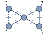
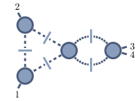
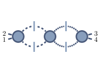
Figure 26: Cuts associated to the labels $c_{4:1;1}$, $c_{4:1;2}$, $c_{4:1;3}$ of the generating set $G_{4:1}$. The cuts of $c_{4:1;1}$ and $c_{4:1;3}$ are invariant under $\rho_{2}\circ\operatorname{Exch}$, and require symmetry factors of $\tfrac{1}{2}$.

Thanks to the separability of the two loops we can first focus our attention on the right-hand loop in each cut. We need to consider only two unique contributions,

(I): $$\text{C}^{(1)}_{\textrm{R}}(\{(3),(4);(),()\},\{();();();()\})\,,$$ (153)

(II): $$\text{C}^{(1)}_{\textrm{R}}(\{(3,4);(),()\},\{();();();()\})$$

as shown in Fig. 27.

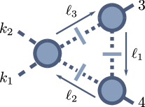
(I) ,          (II) .

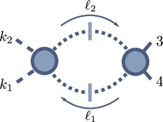
Figure 27: The two unique cuts for the right-hand loop of ${R}^{(2)}_{4:1}$.

For the triangle coefficient (I), we use the loop-momentum parametrization of eqs. (272) and (274), which for the present case of $K_{1}=k_{3}$, $K_{2}=k_{4}$ simplifies to,

$$\ell_{1}^{\mu}=\frac{1}{2}\left(t\mathinner{\langle{4|\gamma^{\mu}|3}]}-\frac{\mu^{2}}{s_{34}t}\mathinner{\langle{3|\gamma^{\mu}|4}]}\right),$$ (154)

$$\ell_{1}^{\ast\mu}=\frac{1}{2}\left(t\mathinner{\langle{3|\gamma^{\mu}|4}]}-\frac{\mu^{2}}{s_{34}t}\mathinner{\langle{4|\gamma^{\mu}|3}]}\right).$$

The routing of the loop momenta used here is shown in Fig. 27. Using the expressions for the scalar tree amplitudes from Appendix B, a brief computation leads to,

$$\hphantom{{}={}}\text{C}^{(1)}_{\textrm{R}}(\{(3),(4);(),()\},\{();();();()\})$$ (155)

$$=\frac{1}{2}\sum_{\ell,\ell^{\ast}}\operatorname{Inf}_{\mu^{2},t}\Big{[}A^{(0)}(k_{1\varphi}k_{2\varphi}\ell_{3{\varphi^{\prime}}}(-\ell_{2})_{{\varphi^{\prime}}})A^{(0)}(3^{+}\ell_{1{\varphi^{\prime}}}(-\ell_{3})_{{\varphi^{\prime}}})A^{(0)}(4^{+}\ell_{2{\varphi^{\prime}}}(-\ell_{1})_{{\varphi^{\prime}}})\Big{]}\Big{|}_{\mu^{2},t^{0}}$$

$$=\frac{1}{2}\operatorname{Inf}_{\mu^{2},t}\Big{[}\sum_{\ell,\ell^{\ast}}\frac{\mathinner{[{3|\ell_{1}|4}\rangle}}{\mathinner{\langle{34}\rangle}}\frac{\mathinner{[{4|\ell_{1}|3}\rangle}}{\mathinner{\langle{43}\rangle}}\frac{L_{k_{1}\ell_{3}}}{s_{34}}\Big{]}\Big{|}_{\mu^{2},t^{0}}$$

$$=\frac{1}{2}\operatorname{Inf}_{\mu^{2},t}\Big{[}\frac{\mu^{2}}{\mathinner{\langle{34}\rangle}^{2}}\Big{(}2L_{k_{1}3}+\Big{(}t\mathinner{\langle{4|k_{1}|3}]}-\frac{\mu^{2}}{s_{34}t}\mathinner{\langle{3|k_{1}|4}]}\Big{)}+\Big{(}t\mathinner{\langle{3|k_{1}|4}]}-\frac{\mu^{2}}{s_{34}t}\mathinner{\langle{4|k_{1}|3}]}\Big{)}\Big{)}\Big{]}\Big{|}_{\mu^{2},t^{0}}$$

$$=\frac{L_{k_{1}3}}{\mathinner{\langle{34}\rangle}^{2}}.$$

For the bubble cut (II) we use the parametrization of eq. (279) with $K=k_{3}+k_{4}$. In addition to the bubble cut, the bubble coefficient (II) in principle requires the contribution from a parent triangle with $K^{\prime}=-k_{3}$. However, choosing the bubble reference momentum $\chi$ in the loop-momentum parametrization of eq. (279) to be $k_{3}$, the integrals $T^{i}$ of eq. (283) vanish. The triangle therefore does not contribute, and only the bubble cut itself is required.

For this choice of $\chi$, the generic bubble loop-momentum parametrization of eq. (279) simplifies to,

$$\ell^{\mu}_{1}=(y-1)k_{4}^{\mu}-yk_{3}^{\mu}+\frac{1}{2}\left(t\mathinner{\langle{4|\gamma^{\mu}|3}]}+\left(\frac{y(1-y)}{t}-\frac{\mu^{2}}{ts_{34}}\right)\mathinner{\langle{3|\gamma^{\mu}|4}]}\right)\,.$$ (156)

The bubble coefficient is then,

$$\hphantom{{}={}}\text{C}^{(1)}_{\textrm{R}}(\{(3,4);(),()\},\{();();();()\})$$ (157)

$$=\operatorname{Inf}_{\mu^{2},y,t}\Big{[}A^{(0)}(k_{1\varphi}k_{2\varphi}l_{2{\varphi^{\prime}}}(-l_{1})_{{\varphi^{\prime}}})A^{(0)}(3^{+}4^{+}(\ell_{1})_{{\varphi^{\prime}}}(-\ell_{2})_{{\varphi^{\prime}}})\Big{]}\Big{|}_{t^{0},y^{i}\to Y_{i},\mu^{2}}$$

$$=-\operatorname{Inf}_{\mu^{2},y,t}\Big{[}\frac{L_{k_{1}(-\ell_{1})}}{s_{34}}\frac{\mu^{2}}{L_{4\ell_{1}}}\frac{\mathinner{[{34}]}}{\mathinner{\langle{34}\rangle}}\Big{]}\Big{|}_{t^{0},y^{i}\to Y_{i},\mu^{2}}$$

$$=\operatorname{Inf}_{\mu^{2},y,t}\Big{[}\frac{\mu^{2}}{y\mathinner{\langle{34}\rangle}^{2}s_{34}}$$

$$\hskip 20.00003pt\times\Big{[}(y-1)L_{k_{1}4}-yL_{k_{1}3}+t\mathinner{[{3|k_{1}|4}\rangle}+\frac{y(1-y)s_{34}-\mu^{2}}{s_{34}t}\mathinner{[{4|k_{1}|3}\rangle}\Big{]}\Big{]}\Big{|}_{t^{0},y^{i}\to Y_{i},\mu^{2}}$$

$$=\frac{L_{k_{1}4}-L_{k_{1}3}}{\mathinner{\langle{34}\rangle}^{2}s_{34}}.$$

In this case the $\operatorname{Inf}_{y}$ operation only yields a $y^{0}$ term, whose parameter integral $Y_{0}$ is $1$.

We can now use these results to compute the three two-loop coefficients,

$$\text{C}^{(2)}(c_{4:1;1}) =\text{C}^{(1)}_{\textrm{L}}\Big{(}\{(1),(2);(),()\},\text{C}^{(1)}_{\textrm{R}}(\{(3),(4);(),()\},\{();();();()\})\Big{)}\,,$$ (158)

$$\text{C}^{(2)}(c_{4:1;2}) =\text{C}^{(1)}_{\textrm{L}}\Big{(}\{(1),(2);(),()\},\text{C}^{(1)}_{\textrm{R}}(\{(3,4);(),()\},\{();();();()\})\Big{)}\,,$$

$$\text{C}^{(2)}(c_{4:1;1}) =\text{C}^{(1)}_{\textrm{L}}\Big{(}\{(1,2);(),()\},\text{C}^{(1)}_{\textrm{R}}(\{(3,4);(),()\},\{();();();()\})\Big{)}\,.$$

$\mathrm{(I)}\quad\includegraphics[width=108.405pt,valign={c}]{4-pt_example/R41/lh_loop_large_triangle_out},\hskip 30.00005pt\mathrm{(II)}\quad\includegraphics[width=121.41306pt,valign={c}]{4-pt_example/R41/lh_loop_large_bubble_out}$

Figure 28: The two distinct unitarity cuts of the right-hand loop that are required for the cut labels of $G_{4:1}$.

The rational parts of $c_{4:1;1}$ and $c_{4:1;2}$ require triangle cuts of the form shown in (I) of Fig. 28. We use the loop-momentum parametrization

$$\ell_{1}^{\mu} =\frac{1}{2}\left(t\mathinner{\langle{2|\gamma^{\mu}|1}]}-\frac{\mu^{2}}{s_{12}t}\mathinner{\langle{1|\gamma^{\mu}|2}]}\right)\,,$$ (159)

$$\ell_{1}^{\ast\mu} =\frac{1}{2}\left(t\mathinner{\langle{1|\gamma^{\mu}|2}]}-\frac{\mu^{2}}{s_{12}t}\mathinner{\langle{2|\gamma^{\mu}|1}]}\right)\,,$$

with the momentum routing shown in Fig. 28 (I). The coefficients of $c_{4:1;1}$ and $c_{4:1;2}$ are then,

$$\begin{split}\text{C}^{(2)}(c_{4:1;1})&=\frac{1}{2}\sum_{\ell_{1},\ell_{1}^{\ast}}\operatorname{Inf}_{\mu^{2},t}\bigg{[}A^{(0)}((-\ell_{3})_{\varphi}1^{+}(\ell_{1})_{\varphi})A^{(0)}((-\ell_{1})_{\varphi}2^{+}(\ell_{2})_{\varphi})\\ &\hskip 100.00015pt\times\text{C}^{(1)}_{\textrm{R}}(\{(3),(4);(),()\},\{();();();()\})\bigg{]}\bigg{]}\bigg{|}_{t^{0},\mu^{2}}\\ &=\frac{1}{2}\frac{s_{12}}{\mathinner{\langle{12}\rangle}^{2}\mathinner{\langle{34}\rangle}^{2}}\sum_{\ell_{1},\ell_{1}^{\ast}}\operatorname{Inf}_{\mu^{2},t}\Big{[}L_{\ell_{3}3}\Big{]}\Big{|}_{t^{0},\mu^{2}}\\ &=\frac{1}{2}\frac{s_{12}}{\mathinner{\langle{12}\rangle}^{2}\mathinner{\langle{34}\rangle}^{2}}\operatorname{Inf}_{\mu^{2},t}\Big{[}\mu^{2}\Big{(}2s_{13}+\Big{(}t\mathinner{\langle{2|3|1}]}-\frac{\mu^{2}}{s_{12}t}\mathinner{\langle{1|3|2}]}\Big{)}\\ &\hskip 150.00023pt+\Big{(}t\mathinner{\langle{1|3|2}]}-\frac{\mu^{2}}{s_{12}t}\mathinner{\langle{2|3|1}]}\Big{)}\Big{)}\Big{]}\Big{|}_{\mu^{2},t^{0}}\\ &=\frac{s_{12}s_{13}}{\mathinner{\langle{12}\rangle}^{2}\mathinner{\langle{34}\rangle}^{2}}\,,\end{split}$$ (160)

$$\begin{split}\text{C}^{(2)}(c_{4:1;2})&=\frac{1}{2}\sum_{\ell_{1},\ell_{1}^{\ast}}\operatorname{Inf}_{\mu^{2},t}\bigg{[}A^{(0)}((-\ell_{3})_{\varphi}1^{+}(\ell_{1})_{\varphi})A^{(0)}((-\ell_{1})_{\varphi}2^{+}(\ell_{2})_{\varphi})\\ &\hskip 100.00015pt\times\text{C}^{(1)}_{\textrm{R}}(\{(3,4);(),()\},\{();();();()\})\bigg{]}\bigg{]}\bigg{|}_{t^{0},\mu^{2}}\\ &=\frac{1}{2}\frac{s_{12}}{\mathinner{\langle{12}\rangle}^{2}\mathinner{\langle{34}\rangle}^{2}}\sum_{\ell_{1},\ell_{1}^{\ast}}\operatorname{Inf}_{\mu^{2},t}\Big{[}L_{\ell_{3}4}-L_{\ell_{3}3}\Big{]}\Big{|}_{t^{0},\mu^{2}}\\ &=\frac{s_{14}-s_{13}}{\mathinner{\langle{12}\rangle}^{2}\mathinner{\langle{34}\rangle}^{2}}\,.\end{split}$$ (161)

The rational contributions of these cuts are then,

$${R}^{(2)}_{c_{4:1;1}}(1,2,3,4) =4I^{(2),D}_{{\textrm{Tri},\textrm{Tri}}}(c_{4:1;1})\,\text{C}^{(2)}(c_{4:1;1})=\text{C}^{(2)}(c_{4:1;1})=\frac{s_{12}s_{13}}{\mathinner{\langle{12}\rangle}^{2}\mathinner{\langle{34}\rangle}^{2}}\,,$$ (162)

$${R}^{(2)}_{c_{4:1;2}}(1,2,3,4) =4I^{(2),D}_{{\textrm{Tri},\textrm{Bub}}}(c_{4:1;2})\,\text{C}^{(2)}(c_{4:1;2})=\frac{s_{12}}{6}\,\text{C}^{(2)}(c_{4:1;2})=\frac{1}{6}\frac{s_{12}(s_{14}-s_{13})}{\mathinner{\langle{12}\rangle}^{2}\mathinner{\langle{34}\rangle}^{2}}\,.$$

For the parameterization of the left loop momentum of $c_{4:1;3}$, we choose $\chi=k_{1}$ as the reference momentum, so that the bubble coefficient again does not require parent-triangle cut contributions. With this parametrization,

$$\ell^{\mu}_{1}=(y-1)k_{2}^{\mu}-yk_{1}^{\mu}+\frac{1}{2}\ \left(t\mathinner{\langle{2|\gamma^{\mu}|1}]}+\left(\frac{y(1-y)}{t}-\frac{\mu^{2}}{ts_{12}}\right)\mathinner{\langle{1|\gamma^{\mu}|2}]}\right).$$ (163)

The two-loop coefficient then evaluates to

$$\text{C}^{(2)}(c_{4:1;3}) =\operatorname{Inf}_{\mu^{2},t,y}\bigg{[}A^{(0)}(1^{+}2^{+}(\ell_{1})_{\varphi}(-\ell_{2})_{\varphi})$$ (164)

$$\hskip 100.00015pt\times\text{C}^{(1)}_{\textrm{R}}(\{(3,4);(),()\},\{();();();()\})\bigg{]}\bigg{]}\bigg{|}_{y^{i}\to Y_{i},t^{0},\mu^{2}}$$

$$=\operatorname{Inf}_{\mu^{2},t,y}\Big{[}\frac{\mathinner{[{12}]}}{\mathinner{\langle{12}\rangle}}\frac{\mu^{2}}{s_{2\ell_{1}}}\frac{L_{4\ell_{2}}-L_{3\ell_{2}}}{\mathinner{\langle{34}\rangle}^{2}s_{34}}\Big{]}\Big{|}_{y^{i}\to Y^{i},t^{0},\mu^{2}}$$

$$=2\frac{s_{13}-s_{14}}{\mathinner{\langle{12}\rangle}^{2}\mathinner{\langle{34}\rangle}^{2}s_{12}}\,.$$

The corresponding rational part is

$${R}^{(2)}_{c_{4:1;3}}(1,2,3,4)=4I^{(2),D}_{{\textrm{Bub},\textrm{Bub}}}(c_{4:1;3})\,\text{C}^{(2)}(c_{4:1;3})=\frac{s_{12}^{2}}{9}\,\text{C}^{(2)}(c_{4:1;3})=\frac{2}{9}\frac{s_{12}(s_{13}-s_{14})}{\mathinner{\langle{12}\rangle}^{2}\mathinner{\langle{34}\rangle}^{2}}\,.$$ (165)

Summing the results of eqs. (162) and (165) with their associated symmetry factors we find,

$$\tilde{{R}}^{(2)}_{4:1}(1^{+}2^{+},3^{+}4^{+})=\frac{5s_{12}s_{23}+s_{23}^{2}}{18\mathinner{\langle{12}\rangle}\mathinner{\langle{23}\rangle}\mathinner{\langle{34}\rangle}\mathinner{\langle{41}\rangle}},$$ (166)

After summing over cyclic permutations of the external kinematics we obtain

$${R}^{(2)}_{4:1}(1^{+}2^{+}3^{+}4^{+})=\sum_{\sigma\in Z_{4}}\tilde{{R}}^{(2)}_{4:1}(\sigma[1,2,3,4])=\frac{s_{13}^{2}+8s_{12}s_{23}}{9\mathinner{\langle{12}\rangle}\mathinner{\langle{23}\rangle}\mathinner{\langle{34}\rangle}\mathinner{\langle{41}\rangle}},$$ (167)

which agrees with the result of refs. [10, 43].

V.1.1 Subleading-color ${R}^{(2)}_{4:3}$

To compute the subleading rational part ${R}^{(2)}_{4:3}(1,2;3,4)$, we construct a generating set following eq. (80),

$$G_{4:3}=\mathrm{AllLabels}^{\{\mathop{\rm ITr}\nolimits(1,2),\mathop{\rm ITr}\nolimits(3,4),N_{c}\}}\cup\mathrm{AllLabels}^{\{\mathop{\rm ITr}\nolimits(3,4),N_{c},\mathop{\rm ITr}\nolimits(1,2)\}}\cup\mathrm{AllLabels}^{\{N_{c},\mathop{\rm ITr}\nolimits(1,2),\mathop{\rm ITr}\nolimits(3,4)\}}\,.$$ (168)

Each of the sets contains four labels,

$$\mathrm{AllLabels}^{\{\mathop{\rm ITr}\nolimits(1,2),\mathop{\rm ITr}\nolimits(3,4),N_{c}\}} =\{c_{4:3;1},c_{4:3;2},c_{4:3;3},c_{4:3;4}\}$$ (169)

$$\mathrm{AllLabels}^{\{\mathop{\rm ITr}\nolimits(3,4),N_{c},\mathop{\rm ITr}\nolimits(1,2)\}} =\{c_{4:3;5},c_{4:3;6},c_{4:3;7},c_{4:3;8}\}$$

$$\mathrm{AllLabels}^{\{N_{c},\mathop{\rm ITr}\nolimits(1,2),\mathop{\rm ITr}\nolimits(3,4)\}} =\{c_{4:3;9},c_{4:3;10},c_{4:3;11},c_{4:3;12}\}$$

which take the form,

The corresponding cuts are shown in Fig. 29. Summing their rational contributions determines $\tilde{{R}}^{(2)}_{4:3}(1^{+}2^{+};3^{+}4^{+})$,

$$\tilde{{R}}^{(2)}_{4:3}(1^{+}2^{+};3^{+}4^{+})=\sum_{c\in G_{4:3}}{R}^{(2)}_{c}(1,2;3,4)\,,$$ (171)

which in turn allows us to compute ${R}^{(2)}_{4:3}(1^{+},2^{+};3^{+},4^{+})$ via,

$${R}^{(2)}_{4:3}(1^{+}2^{+};3^{+}4^{+})=\sum_{\sigma_{1},\sigma_{2}\in Z_{2}}\tilde{{R}}^{(2)}_{4:3}(\sigma_{1}[1,2];\sigma_{2}[3,4]).$$ (172)

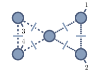
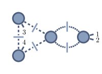
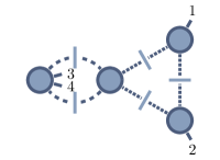
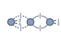
(a) The cut labels $c_{4:3;1}$, $c_{4:3;2}$, $c_{4:3;3}$ and $c_{4:3;4}$ (in order) make up $\mathrm{AllLabels}^{\{\mathop{\rm ITr}\nolimits{1,2},\mathop{\rm ITr}\nolimits{3,4},N_{c}\}}$.

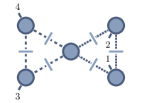
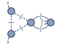
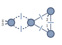
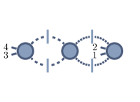
(b) The cut labels $c_{4:3;5}$, $c_{4:3;6}$, $c_{4:3;7}$ and $c_{4:3;8}$ (in order) make up $\mathrm{AllLabels}^{\{\mathop{\rm ITr}\nolimits{3,4},N_{c},\mathop{\rm ITr}\nolimits{1,2}\}}$.

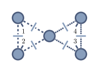
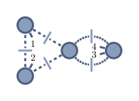
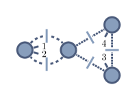
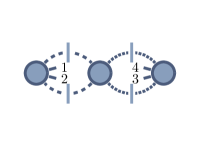
(c) The cut labels $c_{4:3;9}$, $c_{4:3;10}$, $c_{4:3;11}$ and $c_{4:3;12}$ (in order) make up $\mathrm{AllLabels}^{\{N_{c},\mathop{\rm ITr}\nolimits{1,2},\mathop{\rm ITr}\nolimits{3,4}\}}$.

Figure 29: Sets of cut labels that make up the generating set $G_{4:3}$.

Fortunately we do not need to compute these cuts explicitly. Instead we can relate them to the leading-color cuts of eqs. (162) and (165) using the tree-amplitude identities,

$$A^{(0)}(1_{\varphi}2^{+}3_{\varphi})=-A^{(0)}(3_{\varphi}2^{+}1_{\varphi}),\quad A^{(0)}(1_{\varphi}2^{+}3^{+}4_{\varphi})=A^{(0)}(4_{\varphi}3^{+}2^{+}1_{\varphi})\,.$$ (173)

We then find,

Summing these expressions gives,

$$\tilde{{R}}^{(2)}_{4:3}(1,2;3,4)=-\frac{1}{9}\frac{s_{12}}{\mathinner{\langle{12}\rangle}^{2}\mathinner{\langle{34}\rangle}^{2}}(14s_{12}+s_{13})\,.$$ (175)

Carrying out the two cyclic sums of eq. (172), we obtain after some algebra,

$${R}^{(2)}_{4:3}(1^{+}2^{+};3^{+}4^{+}) =-\frac{1}{6}\frac{\mathinner{[{12}]}^{2}}{\mathinner{\langle{34}\rangle}^{2}}$$ (176)

This expression is in agreement with ref. [43].

V.1.2 Subleading-color ${R}^{(2)}_{4:1\mathrm{B}}$

Finally, we determine the subleading-color single-trace rational part ${R}^{(2)}_{4:1\mathrm{B}}$ using the separable approach. The generating set $G_{4:1\text{B}}$ consists of the labels,

which are shown in Fig. 30.

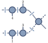
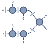
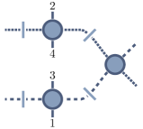
(a) Cuts associated to the labels $c_{4:1\text{B};1}$, $c_{4:1\text{B};2}$, $c_{4:1\text{B};3}$ in $G_{4:1\text{B}}$. These labels are invariant under $\rho_{-1}\circ\text{Rot}$, and therefore require a symmetry factor of $\tfrac{1}{4}$.

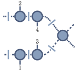
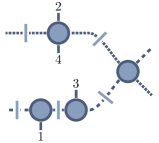
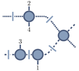
(b) Cuts associated to the labels $c_{4:1\text{B};4}$, $c_{4:1\text{B};5}$, $c_{4:1\text{B};6}$ in $G_{4:1\text{B}}$. These labels are invariant under $\rho_{-2}\circ\text{Rot}^{2}$, and therefore require a symmetry factor of $\tfrac{1}{2}$.

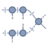
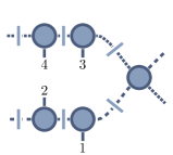
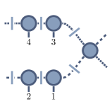
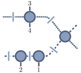
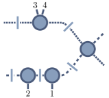
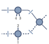
(c) Cuts associated to the labels $c_{4:1\text{B};7},\ldots,c_{4:1\text{B};16}$ in $G_{4:1\text{B}}$. These labels are not invariant under $Z_{4}\times\text{Rot}$, and therefore do not require a symmetry factor.

Figure 30: cut labels in the generating set $G_{4:1\text{B}}$, classified by the symmetry factors they require.

Of these labels, the first six require symmetry factors. The labels $c_{4:1\text{B};1}$, $c_{4:1\text{B};2}$, and $c_{4:1\text{B};3}$ each come with a factor of $\frac{1}{4}$, because

$$\rho_{-1}\circ\text{Rot}[c_{4:1\text{B};i}]=c_{4:1\text{B};i},\quad i=1,2,3\,.$$ (178)

The labels $c_{4:1\text{B};4}$, $c_{4:1\text{B};5}$, and $c_{4:1\text{B};6}$ come with a factor of $\frac{1}{2}$, because

$$\rho_{-2}\circ\text{Rot}^{2}[c_{4:1\text{B};i}]=c_{4:1\text{B};i},\quad i=4,5,6\,.$$ (179)

The remaining cuts are not invariant under $Z_{4}\times\text{Rot}$, and therefore do not require such factors. In summary, we have,

$$S_{c_{4:1\text{B};i}}=\left\{\begin{aligned} &\tfrac{1}{4},\quad&&i=1,2,3,\\ &\tfrac{1}{2},\quad&&i=4,5,6,\\ &1,\quad&&\text{otherwise}.\end{aligned}\right.$$ (180)

We then have

$${R}^{(2)}_{4:1\mathrm{B}}(1^{+}2^{+}3^{+}4^{+})=\sum_{\sigma\in Z_{4}}\tilde{{R}}^{(2)}_{4:1\mathrm{B}}(\sigma[1,2,3,4])\,,$$ (181)

with

$$\tilde{{R}}^{(2)}_{4:1\mathrm{B}}(1,2,3,4)=\sum_{c\in G_{4:1\text{B}}}S_{c}{R}^{(2)}_{c}(1,2,3,4)\,.$$ (182)

To compute the rational contributions ${R}^{(2)}_{c}$ of the cuts $c\in G_{4:1\text{B}}$, we follow the procedure of section III.4.2. We start by computing the one-loop coefficient of loop $2$. Thanks to the amplitude relations of eq. (173), we do not need to compute the coefficient of every cut individually. Instead, we only need to consider three distinct types of cuts. By connecting the scalar line of loop $2$, we can represent them in the familiar form as shown in Fig. 31.

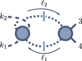
(I)  ,       (II)  ,       (III)  .

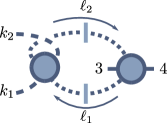
Figure 31: The three distinct unitarity cuts (I, II, III) of loop $2$ needed for the cut labels in $G_{4:1\text{B}}$.

In the label notation, these correspond to the sets

$$\mathrm{(I):} \quad E_{2}=(),(), \qquad E_{4}=(3),(4)\,,$$ (183)

$$\mathrm{(II):} \quad E_{2}=(), \qquad E_{4}=(3,4)\,,$$

$$\mathrm{(III):} \quad E_{2}=(3), \qquad E_{4}=(4)\,,$$

where for all three, $E_{\textrm{C},i}=()$. Using the same loop-momentum parametrization as in eqs. (154) and (156), we obtain for these cuts,

$$\begin{split}&\hphantom{={}}\text{C}^{(1)}_{2}(\{(),();(3),(4)\},\{(),(),(),()\})\\ &=\frac{1}{2}\sum_{\ell,\ell^{\ast}}\operatorname{Inf}_{\mu^{2},t}\Big{[}A^{(0)}(k_{1\varphi}(\ell_{3})_{{\varphi^{\prime}}}k_{2\varphi}(-\ell_{2})_{{\varphi^{\prime}}})A^{(0)}(3^{+}(\ell_{1})_{{\varphi^{\prime}}}(-\ell_{3})_{{\varphi^{\prime}}})\\ &\hskip 85.35826pt\times A^{(0)}(4^{+}(\ell_{2})_{{\varphi^{\prime}}}(-\ell_{1})_{{\varphi^{\prime}}})\Big{]}\Big{|}_{\mu^{2},t^{0}}\\ &=-\frac{1}{2}\operatorname{Inf}_{\mu^{2},t}\Big{[}\sum_{\ell,\ell^{\ast}}\frac{\mathinner{[{3|\ell_{1}|4}\rangle}}{\mathinner{\langle{34}\rangle}}\frac{\mathinner{[{4|\ell_{1}|3}\rangle}}{\mathinner{\langle{43}\rangle}}\Big{]}\Big{|}_{\mu^{2},t^{0}}\\ &=-\operatorname{Inf}_{\mu^{2},t}\Big{[}\frac{\mu^{2}s_{34}}{\mathinner{\langle{34}\rangle}^{2}}\Big{]}\Big{|}_{\mu^{2},t^{0}}\\ &=\frac{\mathinner{[{34}]}}{\mathinner{\langle{34}\rangle}},\end{split}$$ (184)

$$\begin{split}&\hphantom{={}}\text{C}^{(1)}_{2}(\{();(3,4)\},\{(),(),(),()\})\\ &=\operatorname{Inf}_{\mu^{2},y,t}\Big{[}A^{(0)}(k_{1\varphi}(l_{2})_{{\varphi^{\prime}}}k_{2\varphi}(-l_{1})_{{\varphi^{\prime}}})A^{(0)}(3^{+}4^{+}(\ell_{1})_{{\varphi^{\prime}}}(-\ell_{2})_{{\varphi^{\prime}}})\Big{]}\Big{|}_{t^{0},y^{i}\to Y_{i},\mu^{2}}\\ &=\operatorname{Inf}_{\mu^{2},y,t}\Big{[}\frac{\mu^{2}}{L_{4\ell_{1}}}\frac{\mathinner{[{34}]}}{\mathinner{\langle{34}\rangle}}\Big{]}\Big{|}_{t^{0},y^{i}\to Y_{i},\mu^{2}}=\operatorname{Inf}_{\mu^{2},y,t}\Big{[}\frac{\mu^{2}}{y\mathinner{\langle{34}\rangle}^{2}}\Big{]}\Big{|}_{t^{0},y^{i}\to Y_{i},\mu^{2}}=0,\end{split}$$ (185)

$$\begin{split}&\hphantom{={}}\text{C}^{(1)}_{2}(\{(3);(4)\},\{(),(),(),()\})\\ &=\operatorname{Inf}_{\mu^{2},y,t}\Big{[}A^{(0)}(k_{1\varphi}(l_{2})_{{\varphi^{\prime}}}k_{2\varphi}(-l_{1})_{{\varphi^{\prime}}})A^{(0)}(3^{+}(-\ell_{2})_{{\varphi^{\prime}}}4^{+}(\ell_{1})_{{\varphi^{\prime}}})\Big{]}\Big{|}_{t^{0},y^{i}\to Y_{i},\mu^{2}}\\ &=\operatorname{Inf}_{\mu^{2},y,t}\Big{[}\frac{\mu^{2}\mathinner{[{34}]}^{2}}{L_{3\ell_{1}}L_{3\ell_{2}}}\Big{]}\Big{|}_{t^{0},y^{i}\to Y_{i},\mu^{2}}=-\operatorname{Inf}_{\mu^{2},y,t}\Big{[}\frac{\mu^{2}}{y(1-y)\mathinner{\langle{34}\rangle}^{2}}\Big{]}\Big{|}_{t^{0},y^{i}\to Y_{i},\mu^{2}}\\ &=0.\end{split}$$ (186)

The bubble coefficients (II) and (III) would in principle also require the computation of one or two triangle cuts respectively. However, the choice $\chi=k_{3}$ makes such triangle cuts vanish in either case, and the bubble cut again suffices.

As the bubble coefficients (II) and (III) vanish, the rational contributions corresponding to most cut labels in $G_{4:1\text{B}}$ vanish as well. In fact, as the triangle coefficient (I) is independent of $k_{1}$ and $k_{2}$, we can immediately see that any bubble coefficient of loop $1$ has to vanish as well. Thus the only non-vanishing cuts of $\tilde{{R}}^{(2)}_{4:1\mathrm{B}}$ are those of the ${\{{\textrm{Tri},\textrm{Tri}}\}}$ class, specifically $c_{4:1\text{B};1}$, $c_{4:1\text{B};2}$, $c_{4:1\text{B};4}$, $c_{4:1\text{B};7}$, $c_{4:1\text{B};8}$, and $c_{4:1\text{B};9}$. We will see later in Sect. VII.3 that the vanishing of all one-loop squared coefficients except for ${\{{\textrm{Tri},\textrm{Tri}}\}}$ ones is a generic feature of ${R}^{(2)}_{n:1\text{B}}$ rational parts, which holds for any number of external gluons.

Using tree-amplitude relations, we find the following relations between the rational contributions of the labels in $G_{4:1\text{B}}$,

$${R}^{(2)}_{c_{4:1\text{B};1}}={R}^{(2)}_{c_{4:1\text{B};2}}={R}^{(2)}_{c_{4:1\text{B};9}}=-{R}^{(2)}_{c_{4:1\text{B};4}}=-{R}^{(2)}_{c_{4:1\text{B};7}}=-{R}^{(2)}_{c_{4:1\text{B};8}}\,.$$ (187)

We thus only need to determine a single one-loop squared coefficient. We pick $c_{4:1\text{B};9}$. Using the momentum routing already seen in Fig. 28 and parametrization of eq. (159), we can determine the triangle coefficient of loop $1$—and therefore the two-loop coefficient of $c_{4:1\text{B};9}$—to be,

$$\text{C}^{(2)}(c_{4:1\text{B};9}) =\text{C}^{(1)}_{1}(\{(1),(2);(),()\},\text{C}^{(1)}_{2}(\{(),();(3),(4)\},\{(),(),(),()\}))$$ (188)

$$=\frac{1}{2}\sum_{\ell_{1},\ell_{1}^{\ast}}\operatorname{Inf}_{\mu^{2},t}\bigg{[}A^{(0)}((-\ell_{3})_{\varphi}1^{+}(\ell_{1})_{\varphi})A^{(0)}((-\ell_{1})_{\varphi}2^{+}(\ell_{2})_{\varphi})$$

$$\hskip 120.00018pt\times\text{C}^{(1)}_{2}(\{(),();(3),(4)\},\{(),(),(),()\})\bigg{]}\bigg{|}_{t^{0},\mu^{2}}$$

$$=\frac{1}{2}\sum_{\ell_{1},\ell_{1}^{\ast}}\operatorname{Inf}_{\mu^{2},t}\Big{[}\frac{\mathinner{[{1|\ell_{1}|2}\rangle}}{\mathinner{\langle{12}\rangle}}\frac{\mathinner{[{2|\ell_{1}|1}\rangle}}{\mathinner{\langle{21}\rangle}}\frac{\mathinner{[{34}]}}{\mathinner{\langle{34}\rangle}}\Big{]}\Big{|}_{t^{0},\mu^{2}}$$

$$=\frac{\mathinner{[{12}]}\mathinner{[{34}]}}{\mathinner{\langle{12}\rangle}\mathinner{\langle{34}\rangle}}\,.$$

The rational contribution of $c_{4:1\text{B};9}$ is thus,

$${R}^{(2)}_{c_{4:1\text{B};9}}=4I^{(2),D}_{{\textrm{Tri},\textrm{Tri}}}\text{C}^{(2)}(c_{4:1\text{B};9})=\frac{\mathinner{[{12}]}\mathinner{[{34}]}}{\mathinner{\langle{12}\rangle}\mathinner{\langle{34}\rangle}}\,.$$ (189)

Combining this result with the relations of eq. (187) and the symmetry factors of eq. (180), we find

$$\tilde{{R}}^{(2)}_{4:1\mathrm{B}}(1^{+}2^{+}3^{+}4^{+}) =\frac{1}{4}\left[{R}^{(2)}_{c_{4:1\text{B};1}}+{R}^{(2)}_{c_{4:1\text{B};2}}\right]+\frac{1}{2}{R}^{(2)}_{c_{4:1\text{B};4}}+{R}^{(2)}_{c_{4:1\text{B};7}}+{R}^{(2)}_{c_{4:1\text{B};8}}+{R}^{(2)}_{c_{4:1\text{B};9}}$$ (190)

$$=\frac{\mathinner{[{12}]}\mathinner{[{34}]}}{\mathinner{\langle{12}\rangle}\mathinner{\langle{34}\rangle}}\left[\frac{2}{4}+\frac{1}{2}-1-1+1\right]=0\,,$$

and as a consequence,

$${R}^{(2)}_{4:1\mathrm{B}}(1^{+}2^{+}3^{+}4^{+})=\sum_{\sigma\in Z_{4}}\tilde{{R}}^{(2)}_{4:1\mathrm{B}}(\sigma(1,2,3,4))=0\,.$$ (191)

This is again in agreement with the result of refs. [42, 43].

VI Mathematica Implementation

To verify the one-loop squared approach against literature results beyond four points, we automated the generation of cuts and symmetry factors required for the generating sets $G_{n:1}$, $G_{n:i}$, $G_{n:r,k}$ and $G_{n:1\text{B}}$ in Mathematica. The code is general, and able to produce generating sets for an arbitrary number of gluons.

We wrote a set of Mathematica packages to automate the evaluation of unitarity cuts on specified (rational) kinematic points. These packages are extensions of the SpinorHelicity6D package of ref. [56], which provides an implementation of the four- and six-dimensional spinors.

To determine the integral coefficients as reviewed in App. F, we require an implementation of the $\operatorname{Inf}$ operation. As a reminder, given a function $f(x)$ that scales like $x^{p}$ for $x\to\infty$, we obtain $\operatorname{Inf}_{x}[f(x)])$ from its series expansion around large values of $x$,

$$f(x)=\sum_{i=0}^{p}c_{i}x^{i}+\mathcal{O}\left(\frac{1}{x}\right)\equiv\operatorname{Inf}_{x}[f(x)]+\mathcal{O}\left(\frac{1}{x}\right)\,.$$ (192)

We use Mathematica to perform these series expansions symbolically. While this approach is not optimal numerically, it retains full flexibility in choosing the kinematics. We can use rational kinematics to make exact comparisons with literature results. We can also make use of the symbolic capabilities of Mathematica on partially or fully parametrized kinematics. Examples of the latter include the verifying collinear behavior exactly, obtaining analytic results from completely parametrized kinematics, and analyzing the large-$z$ behavior under a BCFW shift.

The products of trees in $D$-dimensional unitarity cuts are always rational functions in the loop-momentum parameters $\mu^{2}$, $t$ and $y$, with coefficients generically algebraic in the external kinematics. A potential problem that arises when carrying out the series expansions symbolically is the appearance of deeply nested intermediate expressions. These can appear in the evaluation of cuts even for purely numerical kinematic points. We therefore avoid Mathematica’s built-in Series and SeriesCoefficient, using instead our own implementation of these functions RationalSeries and RationalSeriesCoefficient. They are optimized for expansions of rational functions. Our functions perform the series expansions recursively, caching intermediate results for improved performance.

In addition, we store any coefficients depending only on the external kinematics in symbolic objects called NumSymb. These can be defined recursively, and depend on NumSymb objects of previous steps in the computation. The NumSymb objects can therefore be arranged in a directed acyclic graph. Each NumSymb represents an algebraic number for purely numerical kinematics, and an algebraic function of the parameters in parametrized kinematics. We assign the same NumSymb for repeated appearances of a specific subexpression, so that every NumSymb represents a unique kinematic structure. We also avoid unnecessary computations by performing a zero test on each newly defined NumSymb object; the Mathematica function PossibleZeroQ does this efficiently and exactly, given the option Method->ExactAlgebraics. For this zero test we set all kinematic parameters to random integer values of sufficient size to avoid accidental cancellations.

For cut coefficients, only the final result is known to be rational in the kinematics: on purely numeric rational kinematic points it will be a rational number, while for rational kinematics involving analytic parameters, it is a rational function in these parameters. Intermediate expressions generically involve square roots, which are only guaranteed to cancel in the final result. Performing simplifications in intermediate steps is therefore costly. Furthermore, the final result will not necessarily depend on all of the NumSymb objects, as they may cancel or contribute only to powers in the loop-momentum parameters not required for the desired coefficient. We therefore perform the series expansion without any simplifications along the way, storing the kinematic dependence in the NumSymb objects mentioned before. The end result of the expansion will be a single NumSymb object. We then simplify the result by traversing the dependency graph of this final NumSymb object, performing simplifications from the bottom up, or depth-first. This ensures that we perform only simplifications required for the final result, and that every subexpression is processed only once.

VII Higher-Point Amplitudes

Following our earlier presentation of the separable approach in the example of the four-gluon partial amplitudes, we turn to a discussion of higher-multiplicity results and their comparison to expressions available in the literature. Explicit forms for the generating sets of cut label for up to nine gluons can be found in the auxiliary files provide with this article.

VII.1 The Five-Gluon Amplitude Analytically

The color decomposition of the five-gluon amplitude has the form

$$\mathcal{A}^{(2)}(1^{+}2^{+}3^{+}4^{+}5^{+}) =N_{c}^{2}\sum_{\sigma\in{S_{5}}/{Z_{5}}}\mathop{\rm ITr}\nolimits(\sigma(1,2,3,4,5))A^{(2)}_{5:1}(\sigma(1,2,3,4,5))$$ (193)

$$\hphantom{{}={}}+N_{c}\sum_{\sigma\in{S_{5}}/{P_{5:3}}}\mathop{\rm ITr}\nolimits(\sigma(1,2))\mathop{\rm ITr}\nolimits(\sigma(3,4,5))A^{(2)}_{5:3}(\sigma(1,2);\sigma(3,4,5))$$

$$\hphantom{{}={}}+\sum_{\sigma\in{S_{5}}/{Z_{5}}}\mathop{\rm ITr}\nolimits(\sigma(1,2,3,4,5))A^{(2)}_{5:1\text{B}}(\sigma(1,2,3,4,5))\,.$$

Just as in the four-gluon case, we require the rational parts of three partial amplitudes: ${R}^{(2)}_{5:1}$, ${R}^{(2)}_{5:3}$, and ${R}^{(2)}_{5:1\mathrm{B}}$. Following the discussion of section III, we build generating sets $G_{5:1}$, $G_{5:3}$, $G_{5:11\text{B}}$, which contain $12$, $62$, and $133$ unitarity cuts respectively. The cuts of $G_{5:1}$ and $G_{5:3}$ are shown in Figures 32, 33, and 34, while those of $\tilde{{R}}^{(2)}_{5:1\mathrm{B}}$ are not shown on account of their large number. We include the labels of the cuts in the three generating sets in auxiliary files. For an odd number of momenta, none of the cuts require symmetry factors.

Beginning with five-gluon amplitudes, we rely on our implementation in Mathematica to compute the unitarity cuts due to their increased number and complexity. As our code is able to perform computations symbolically, we evaluated the cuts using parametrized kinematics obtained from momentum twistors, giving us analytic results. In Appendix E we provide the details of this parameterization. We provide the computed expressions for $\tilde{{R}}^{(2)}_{5:1}$, $\tilde{{R}}^{(2)}_{5:3}$ and $\tilde{{R}}^{(2)}_{5:1\text{B}}$ in the auxiliary files.

We verify our approach using the known results for the three partial amplitudes of refs. [20, 25, 33]. Our expressions are in numerical agreement with these results and satisfy the color relations laid out in ref. [70].

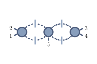
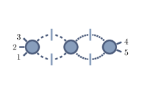
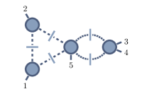
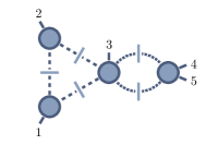
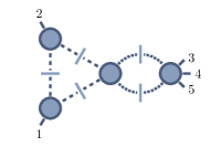
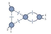
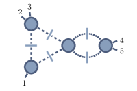
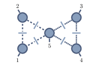
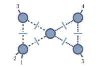
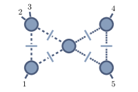
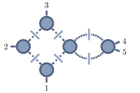
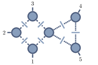
Figure 32: Unitarity cuts in the generating set $G_{5:1}$ of the leading-color rational part ${R}^{(2)}_{5:1}$.

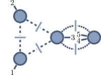
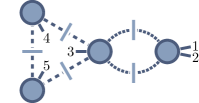
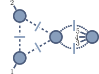
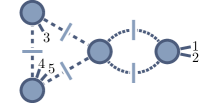
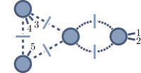
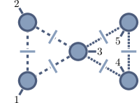
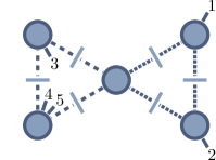
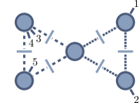
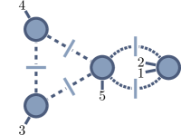
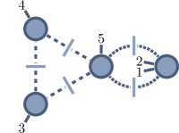
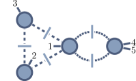
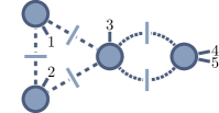
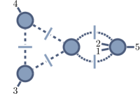
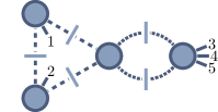
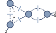
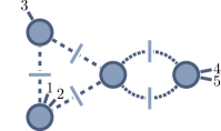
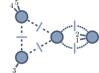
Figure 33: The first $31$ unitarity cuts in the generating set $G_{5:3}$ of ${R}^{(2)}_{5:3}$.

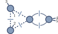
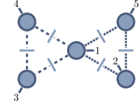
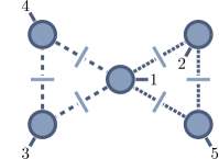
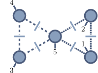
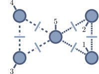
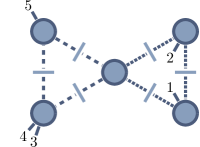
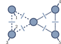
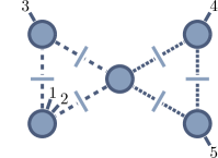
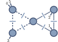
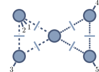
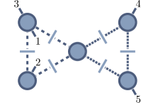
Figure 34: The remaining $31$ unitarity cuts in the generating set $G_{5:3}$ of ${R}^{(2)}_{5:3}$.

VII.2 The Six- and Seven-Gluon Amplitudes: Numeric Results

For $n=6,7$, the two-loop color decomposition has the form,

$$\hphantom{={}}\mathcal{A}^{(2)}(1^{+}2^{+}3^{+}4^{+}5^{+}\ldots n^{+})$$ (194)

$$=N_{c}^{2}\sum_{\sigma\in{S_{n}}/{Z_{n}}}\mathop{\rm ITr}\nolimits(\sigma(1,2,3,4,5,\ldots,n))A^{(2)}_{n:1}(\sigma(1,2,3,4,5,\ldots,n))$$

$$\hphantom{{}={}}+N_{c}\sum_{\sigma\in{S_{n}}/{P_{n:3}}}\mathop{\rm ITr}\nolimits(\sigma(1,2))\mathop{\rm ITr}\nolimits(\sigma(3,4,5,\ldots))A^{(2)}_{n:3}(\sigma(1,2);\sigma(3,4,5,\ldots,n))$$

$$\hphantom{={}}+N_{c}\sum_{\sigma\in{S_{n}}/{P_{n:4}}}\mathop{\rm ITr}\nolimits(\sigma(1,2,3))\mathop{\rm ITr}\nolimits(\sigma(4,5,\ldots))A^{(2)}_{n:4}(\sigma(1,2,3);\sigma(4,5,\ldots,n))$$

$$\hphantom{={}}+\sum_{\sigma\in{S_{n}}/{P_{n:2,2}}}\mathop{\rm ITr}\nolimits(\sigma(1,2))\mathop{\rm ITr}\nolimits(\sigma(3,4))\mathop{\rm ITr}\nolimits(\sigma(5,\ldots,n))A^{(2)}_{n:2,2}(\sigma(1,2);\sigma(3,4);\sigma(5,\ldots,n))$$

$$\hphantom{={}}+\sum_{\sigma\in{S_{n}}/{Z_{n}}}\mathop{\rm ITr}\nolimits(\sigma(1,2,3,4,5,\ldots,n))A^{(2)}_{n:1\text{B}}(\sigma(1,2,3,4,5,\ldots,n))\,.$$

For six and seven gluons, we therefore have to determine five types of rational parts: ${R}^{(2)}_{n:1}$, ${R}^{(2)}_{n:3}$, ${R}^{(2)}_{n:4}$, ${R}^{(2)}_{n:2,2}$ and ${R}^{(2)}_{n:1\text{B}}$. While closed form expressions of these are known in the six-gluon case [25, 24], for seven gluons only ${R}^{(2)}_{7:1}$ has been determined through direct computation [22, 23].

We determine the generating sets of for these rational parts using our automated code. The sizes of these sets are given in Table 1. The cuts of the generating set $G_{6:1}$ are shown in Figs. 35 and 36. It also lists the number of cuts in all generating sets up for up to nine gluons. The reader may find all generating sets in machine-readable form in the auxiliary files.

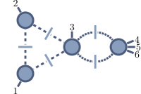
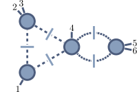
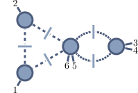
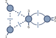
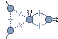
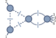
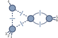
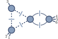
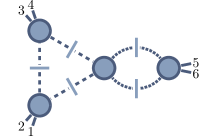
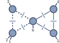
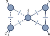
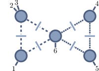
Figure 35: The first 24 unitarity cuts in the generating set $G_{6:1}$ of ${R}^{(2)}_{6:1}$.

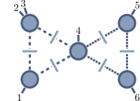
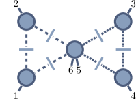
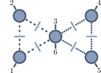
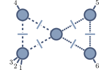
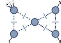
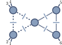
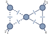
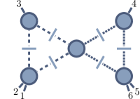
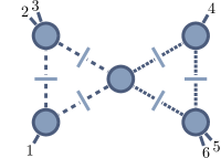
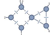
Figure 36: The remaining 23 unitarity cuts in the generating set $G_{6:1}$ of ${R}^{(2)}_{6:1}$.

Using our Mathematica implementation, we compute ${R}^{(2)}_{6:1}$, ${R}^{(2)}_{6:3}$, ${R}^{(2)}_{6:2,2}$, ${R}^{(2)}_{6:1\text{B}}$ and ${R}^{(2)}_{7:1\text{B}}$ numerically on rational kinematic points using the separable approach. In all cases, we find exact agreement with the analytic expressions reported in the literature.

$n$	$4$	$5$	$6$	$7$	$8$	$9$
$\tilde{{R}}^{(2)}_{n:1}$	$3(7)$	$12(33)$	$47(149)$	$126(413)$	$315(1083)$	$676(2314)$
$\tilde{{R}}^{(2)}_{n:3}$	$12(27)$	$62(171)$	$242(729)$	$773(2440)$	$2111(6801)$	$5101(16479)$
$\tilde{{R}}^{(2)}_{n:4}$	—	—	$240(735)$	$768(2422)$	$2163(6879)$	$5459(17315)$
$\tilde{{R}}^{(2)}_{n:2,2}$	—	—	$1023(3168)$	$3300(10760)$	$8911(29120)$	$21694(69696)$
$\tilde{{R}}^{(2)}_{n:5}$	—	—	—	—	$2099(6621)$	$5259(16414)$
$\tilde{{R}}^{(2)}_{n:2,3}$	—	—	—	—	$9893(32860)$	$25044(81730)$
$\tilde{{R}}^{(2)}_{n:3,3}$	—	—	—	—	—	$28242(93576)$
$\tilde{{R}}^{(2)}_{n:1\mathrm{B}}$	$16(42)$	$133(385)$	$847(2678)$	$3909(12751)$	$15199(50078)$	$51030(165603)$

Table 1: The number of cuts in the generating sets defined in eqs. (61), (84) and (98) for all rational parts of partial amplitudes with up to nine gluons. Bubble coefficients require additional triangle cuts, and we indicate the total number of cuts including these triangles in parenthesis.

VII.3 Subleading-Color Single-Trace Rational Parts in the Separable Approach

DPS conjectured an all-multiplicity form [33] for the subleading single-trace amplitudes ${R}^{(2)}_{n:1\text{B}}$, making them the first two-loop Yang–Mills amplitudes (conjecturally) known for an arbitrary number of gluons. This conjecture is possible due to special properties of these amplitudes. These properties lead to a simpler form, easier to determine than that of the remaining color-ordered amplitudes.

A significant simplification is the absence of multi-particle poles in these rational parts. This property was first observed in ref. [33]. Here we provide an argument from the point of view of the separable approach. In addition, as we shall see below, in the separable approach, all but triangle cuts of ${R}^{(2)}_{n:1\text{B}}$ vanish. We already observed this fact in the derivation of ${R}^{(2)}_{4:1\text{B}}$ in Sect. V. We provide a general argument based on power counting, specializing the analysis given in Appendix A of ref. [30]. Finally we discuss high-multiplicity agreement of the conjecture stated in ref. [33] and our computations using the separable approach.

VII.3.1 Absence of Multi-Particles Poles

A striking feature of the $1\text{B}$ amplitudes is the absence of multi-particle poles, as well as the absence of double poles on complex momentum configurations. This feature was exploited in the DPS conjecture by requiring the correct two-particle factorization behavior.

In the separable approach, multi-particle poles can only originate from two-scalar amplitudes of the type $A^{(2)}_{2s}$. For the all-plus helicity configuration, only a factorization of the form $A^{(1)}_{1s}\times A^{(1)}_{1s}$ is allowed, as for the factorizations $A^{(2)}_{2s}\times A^{(0)}$ and $A^{(0)}\times A^{(2)}_{2s}$ the tree amplitude vanishes. For $K=k_{i}+\ldots+k_{i+m}$ going on shell, $A^{(2)}_{2s}$ factorizes along the gluon propagator connecting the two loops,

$$A^{(2)}_{2s}(1^{+}2^{+}\ldots i^{+}\ldots(i+m)^{+}\ldots n^{+})\ \overset{s_{i\mathellipsis i+m}=K^{2}\to 0}{\longrightarrow}\\ \sum_{h=\pm}A^{(1)}_{1s}(1^{+}2^{+}\mathellipsis K^{h}\mathellipsis n^{+})\frac{1}{K^{2}}A^{(1)}_{1s}(i^{+}\mathellipsis(i+m)^{+}(-K)^{\overline{h}})$$ (195)

As $A^{(2)}_{\times}$ does not possess such a propagator, it is finite in this limit. However, we saw that the rational parts ${R}^{(2)}_{n:1\text{B}}$ only receive contributions from $A^{(2)}_{\times}$, as the color structure is incompatible with $A^{(2)}_{2s}$. We can therefore conclude, that ${R}^{(2)}_{n:1\text{B}}$ does not contain any multi-particle poles, in agreement with the findings of ref. [33].

The absence of multi-particle poles in $A^{(2)}_{\times}$ further implies, that the complexity seen in rational parts of the remaining partial amplitudes stems from $A^{(2)}_{2s}$. The fact that $A^{(2)}_{2s}$ is a quantity derivable from scalar QCD may be of use in studying its all-multiplicity behavior.

VII.3.2 Vanishing Cuts

In the one-loop squared construction of the subleading single-trace rational parts ${R}^{(2)}_{n:1\text{B}}$ we find numerically that all cuts except those of the double-triangle class vanish. We can view this as a consequence of a more general principle: the only cut coefficients that contribute to the rational parts ${R}^{(2)}_{\times}$ are of the ${\{{\textrm{Tri},\textrm{Tri}}\}}$ type. The coefficients of one-loop squared integrals involving boxes or bubbles vanish. As ${R}^{(2)}_{n:1\text{B}}$ is made up entirely of ${R}^{(2)}_{\times}$, this rational part can be reduced to products of triangle integrals with appropriate coefficients.

The vanishing of box and bubble coefficients can be understood from power counting arguments. While a gluon coupling to a scalar line contributes one power of the loop momentum to the integrands numerator, the contact term does not. To see explicitly that this leads to the vanishing of box and bubble cuts, we follow the analysis found in Appendix A of Ref. [30], with the requirement that one of the vertices is a contact term.

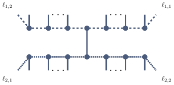
(a) A diagram in the four-scalar amplitude $A^{(0)}_{\mathrm{gluon}}$.

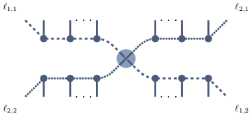
(b) A diagram in the four-scalar amplitude $A^{(0)}_{\mathrm{contact}}$, as it appears in ${R}^{(2)}_{n:1\text{B}}$.

Figure 37: Examples of Feynman diagrams contributing to four-scalar tree amplitudes, that are leading in the large-loop-momentum limit for both loops.

Let us first consider a box cut of one of the loops. We need to determine

$$\operatorname{Inf}_{\mu^{2}}\left[A^{(0)}_{1}A^{(0)}_{2}A^{(0)}_{3}A^{(0)}_{4}\right]_{\mu^{4}}.$$ (196)

Expanding the loop momentum of eq. (264) in the large-$\mu^{2}$ limit, we find that it can generally be expressed as,

$$\ell^{\nu}_{\mathrm{Box}}=\alpha_{1}^{\nu}+\alpha_{2}^{\nu}\sqrt{\mu^{2}}+\frac{1}{\sqrt{\mu^{2}}}\alpha_{3}^{\nu}+\mathcal{O}\bigg{(}\frac{1}{\sqrt{\mu^{2}}^{3}}\bigg{)}\,,$$ (197)

where the $\alpha^{\nu}_{i}$ depend only on the external kinematics. Of the the four amplitudes $A^{(0)}_{i}$, three are of the two-scalar type, while one is the four-scalar central amplitude connecting the loops. In the large-loop-momentum limit, each cubic gluon vertex on the scalar line provides a power of $\ell_{\mathrm{Box}}$. Due to the on-shell condition $\ell_{\mathrm{Box}}^{2}=0$, each scalar propagator carrying the loop momentum contributes $1/\ell_{\mathrm{Box}}$. The dominant contribution (with no special choice of helicity reference momentum) arises from those Feynman diagrams in the tree amplitudes where the ratio of number of gluon-scalar-scalar vertices to scalar propagators is maximal. Examples of such Feynman diagrams for $A^{(0)}_{\mathrm{gluon}}$ and $A^{(0)}_{\mathrm{contact}}$ are shown in Fig. 37.

A product $P^{m}_{\mathrm{Box}}$ of $m$ powers of $\ell_{\mathrm{Box}}$ has the generic form

$$P^{m}_{\mathrm{Box}}(x)=\sum_{i=-m}^{m}x_{i}\left(\sqrt{\mu^{2}}\right)^{i}$$ (198)

In a box cut involving a four-scalar gluon-exchange amplitude $A^{(0)}_{\mathrm{gluon}}$ we obtain the same power counting as in the analysis of ref. [30]. The dominant terms in such terms involve diagrams of the form shown in Fig. 37(a). Determining the box coefficient, up to prefactors that depend on the external kinematics we obtain,

$$\operatorname{Inf}_{\mu^{2}}\left[\frac{P^{m}_{\mathrm{Box}}(x)}{P^{m-4}_{\mathrm{Box}}(y)}\right]_{\mu^{4}}=\frac{x_{m}}{y_{m-4}}\,.$$ (199)

If however a contact-term amplitude $A^{(0)}_{\mathrm{contact}}$ connects the loops, the contact term takes the place of one gluon-scalar-scalar vertex on each scalar line. This shifts the ratio of powers of loop momenta in the numerator and denominator. The leading terms have one fewer power of $\ell_{\mathrm{Box}}$ in the numerator compared to gluon-exchange case, so that

$$\operatorname{Inf}_{\mu^{2}}\left[\frac{P^{m-1}_{\mathrm{Box}}(x)}{P^{m-4}_{\mathrm{Box}}(y)}\right]_{\mu^{4}}=0\,.$$ (200)

Thus, any box cut involving the four-scalar contact term has to vanish.

We can perform the same analysis for bubble cuts to see that they too vanish in the presence of a contact term. The parametrized bubble loop momentum of eq. (279) can be written as

$$\ell_{\mathrm{Bubble}}^{\nu}=\alpha_{1}^{\nu}+y\alpha_{2}^{\nu}+t\alpha_{3}^{\nu}+\frac{y}{t}\alpha_{4}^{\nu}+\frac{y^{2}}{t}\alpha_{5}^{\nu}+\frac{\mu^{2}}{t}\alpha_{6}^{\nu}\,,$$ (201)

while an $m$-fold product $P^{m}_{\mathrm{Bubble}}(x)$ has the generic form

$$P^{m}_{\mathrm{Bubble}}(x)=\sum_{i=0}^{m}\sum_{j=-m}^{m-2i}\sum_{k=\max(0,-j-i)}^{m-j-2i}x_{i,j,k}\,\mu^{2i}t^{j}y^{k}\,.$$ (202)

If the four-scalar amplitude in the bubble cut is of the gluon-exchange type, the leading part of the cut is made up of terms of the form,

$$\operatorname{Inf}_{y,t,\mu^{2}}\left[\frac{P^{m}_{\mathrm{Bubble}}(x)}{P^{m-2}_{\mathrm{Bubble}}(y)}\right]_{y^{i}\to Y_{i},t^{0},\mu^{2}}.$$ (203)

The expanded, generally non-vanishing, form of eq. (203) can be found in ref. [30]. If a four-scalar amplitude $A^{(0)}_{\mathrm{contact}}$ is present, the power of loop momentum in the numerator is again reduced by one. The bubble cut then behaves as

$$\operatorname{Inf}_{y,t,\mu^{2}}\left[\frac{P^{m-1}_{\mathrm{Bubble}}(x)}{P^{m-2}_{\mathrm{Bubble}}(y)}\right]_{y^{i}\to Y_{i},t^{0},\mu^{2}}=0\,,$$ (204)

meaning that such cuts also vanish for a contact-term.

That leaves us with only triangle cuts. There are two types of such cuts: those that contribute to the coefficients of triangle basis integrals, and those required for coefficients of bubble integrals. In either case, the parametrization of the loop momentum of eqs. (272) and (274) can be written as

$$\ell_{\mathrm{Triangle}}^{\nu}=\alpha_{1}^{\nu}+t\alpha_{2}^{\nu}+\frac{1}{t}\alpha_{3}^{\nu}+\frac{\mu^{2}}{t}\alpha_{4}^{\nu}\,,$$ (205)

with a generic $m$-fold product being

$$P^{m}_{\mathrm{Triangle}}(x)=\sum_{i=0}^{m}\sum_{j=-m}^{m-2i}x_{i,j}\,\mu^{2i}t^{j}\,.$$ (206)

For a four-scalar amplitude with a gluon exchange, we find that triangle coefficients receive contributions of the form

$$\operatorname{Inf}_{t,\mu^{2}}\left[\frac{P^{m}_{\mathrm{Triangle}}(x)}{P^{m-3}_{\mathrm{Triangle}}(y)}\right]_{t^{0},\mu^{2}}\\ =\frac{x_{1,m-3}}{y_{0,m-3}}-\frac{x_{0,m}y_{1,m-6}}{y_{0,m-3}^{2}}-\frac{x_{0,m-1}y_{1,m-5}}{y_{0,m-3}^{2}}+\frac{2x_{0,m}y_{0,m-4}y_{1,m-5}}{y_{0,m-3}^{3}}-\frac{x_{1,m-2}y_{0,m-4}}{y_{0,m-3}^{2}}$$ (207)

while those of bubble coefficients are

$$\operatorname{Inf}_{t,\mu^{2}}\left[\frac{P^{m}_{\mathrm{Triangle}}(x)}{P^{m-3}_{\mathrm{Triangle}}(y)}\right]_{t^{i}\to T_{i},\mu^{2}}=c_{1}\left(\frac{x_{1,m-2}}{y_{0,m-3}}-\frac{x_{0,m}y_{1,m-5}}{y_{0,m-3}^{2}}\right)+c_{3}\left(\frac{x_{0,m}}{y_{0,m-3}}\right)$$ (208)

The $c_{i}$ are kinematic factors originating from the $T_{i}$ parameter integrals. On the other hand, for a contact term tree amplitude we find respectively

$$\operatorname{Inf}_{t,\mu^{2}}\left[\frac{P^{m-1}_{\mathrm{Triangle}}(x)}{P^{m-3}_{\mathrm{Triangle}}(y)}\right]_{t^{0},\mu^{2}}=\frac{x_{1,m-3}}{y_{0,m-3}}-\frac{x_{0,m-1}y_{1,m-5}}{y_{0,m-3}^{2}}$$ (209)

and

$$\operatorname{Inf}_{t,\mu^{2}}\left[\frac{P^{m}_{\mathrm{Triangle}}(x)}{P^{m-3}_{\mathrm{Triangle}}(y)}\right]_{t^{i}\to T_{i},\mu^{2}}=0.$$ (210)

We can therefore see that for any one-loop amplitude requiring a contact term, only the coefficients of triangle integrals are non-vanishing. In our setting, this implies that only coefficients of the bowtie integral are nonvanishing in the rational terms of the subleading-color single-trace two-loop amplitude.

VII.3.3 Comparison with Conjecture for ${R}^{(2)}_{7:1\mathrm{B}}$ ${R}^{(2)}_{8:1\mathrm{B}}$ and ${R}^{(2)}_{9:1\mathrm{B}}$

The five- and six-gluon rational terms ${R}^{(2)}_{5:1\text{B}}$, ${R}^{(2)}_{6:1\text{B}}$ to which we have compared our results are known from explicit computations in refs. [34]. Starting from the seven-gluon case, ${R}^{(2)}_{n:1\text{B}}$ is only known in the form of the all-$n$ conjecture of ref. [33].

We can use the separable approach to provide an independent cross-check of this result. Finding agreement would provide evidence for both the correctness of the the conjecture of ref. [33], while at the same time validating the use of the separable approach in the computation of the rational contributions ${R}^{(2)}_{n:1\mathrm{B}}$.

We first consider the seven gluon rational terms ${R}^{(2)}_{7:1\text{B}}$. By specializing the all-$n$ form of ref. [33] to $n=7$ we obtain

$${R}^{(2)}_{7:1\mathrm{B}}={R}^{(2)}_{7:1\mathrm{B},1}+{R}^{(2)}_{7:1\mathrm{B},2}\,,$$ (211)

where,

$${R}^{(2)}_{7:1\mathrm{B},1}=2\frac{\sum_{1\leq i<j<k<l\leq 7}\text{tr}_{5}(ijkl)}{\mathinner{\langle{12}\rangle}\mathinner{\langle{23}\rangle}\mathinner{\langle{34}\rangle}\mathinner{\langle{45}\rangle}\mathinner{\langle{56}\rangle}\mathinner{\langle{67}\rangle}\mathinner{\langle{71}\rangle}}$$ (212)

$${R}^{(2)}_{7:1\mathrm{B}2}=$$

$$-4\Big{[} C_{3745}\text{tr}_{5}[(1+2+3)547]-C_{3746}\text{tr}_{5}[(1+2+3)647]+C_{3756}\text{tr}_{5}[(1+2+3)657]$$

$$+C_{2634}\text{tr}_{5}[(1+2)43(6+7)]+C_{2734}\text{tr}_{5}[(1+2)437]-C_{2635}\text{tr}_{5}[(1+2)53(6+7)]$$

$$-C_{2735}\text{tr}_{5}[(1+2)537]+C_{2645}\text{tr}_{5}[(1+2)54(6+7)]+C_{2745}\text{tr}_{5}[(1+2)547]$$

$$+C_{2736}\text{tr}_{5}[(1+2)637]-C_{2746}\text{tr}_{5}[(1+2)647]+C_{2756}\text{tr}_{5}[(1+2)657]$$

$$+C_{1523}\text{tr}_{5}[132(5+6+7)]+C_{1623}\text{tr}_{5}[132(6+7)]+C_{1723}\text{tr}_{5}[1327]$$

$$-C_{1524}\text{tr}_{5}[142(5+6+7)]-C_{1624}\text{tr}_{5}[142(6+7)]-C_{1724}\text{tr}_{5}[1427]$$

$$+C_{1534}\text{tr}_{5}[143(5+6+7)]+C_{1634}\text{tr}_{5}[143(6+7)]+C_{1734}\text{tr}_{5}[1437]$$

$$+C_{1625}\text{tr}_{5}[152(6+7)]+C_{1725}\text{tr}_{5}[1527]-C_{1635}\text{tr}_{5}[153(6+7)]$$

$$-C_{1735}\text{tr}_{5}[1537]+C_{1645}\text{tr}_{5}[154(6+7)]+C_{1745}\text{tr}_{5}[1547)]-C_{1726}\text{tr}_{5}[1627]$$

$$+C_{1736}\text{tr}_{5}[1637]-C_{1746}\text{tr}_{5}[1647]+C_{1756}\text{tr}_{5}[1657]\Big{]}.$$

Here, we have introduced,

$$\text{tr}_{5}(ijkl)=\text{tr}_{-}(ijkl)-\text{tr}_{+}(ijkl)\,;$$ (213)

we also define,

$$\text{tr}_{-}(ijkl) =\mathinner{\langle{i|jkl|i}]}\,,$$ (214)

$$\text{tr}_{+}(ijkl) =\mathinner{[{i|jkl|i}\rangle}\,.$$

The $C_{rsij}$ are sums over terms with Parke–Taylor denominators,

$$C_{rsij}=\sum_{\alpha\in S_{rsij}}\operatorname{C_{PT}}(1,\mathellipsis,r,j,\{\alpha\},i,s\mathellipsis,7),$$ (215)

where

$$\operatorname{C_{PT}}(a_{1},\mathellipsis,a_{n})=\frac{1}{\langle\!\langle a_{1}a_{2}\mathellipsis a_{7}\rangle\!\rangle}\,.$$ (216)

Here we introduce the notation,

$$\langle\!\langle a_{1}a_{2}\mathellipsis a_{n}\rangle\!\rangle=\mathinner{\langle{a_{1}a_{2}}\rangle}\mathinner{\langle{a_{2}a_{3}}\rangle}\mathellipsis\mathinner{\langle{a_{n-1}a_{n}}\rangle}\mathinner{\langle{a_{n}a_{1}}\rangle}\,.$$ (217)

Define the sets $S_{1}$, $S_{2}$ and $S_{3}$ by splitting $\{1,\mathellipsis,7\}$ as follows,

$$\{1,\mathellipsis,7\}=\{1,\mathellipsis,r\}\cup S_{1}\cup\{i\}\cup S_{2}\cup\{j\}\cup S_{3}\cup\{s,\mathellipsis,7\},$$ (218)

the sets $S_{rsij}$ are obtained via the shuffle product,

$$S_{rsij}=S_{1}\shuffle S_{2}^{T}\shuffle S_{3},$$ (219)

with the transposition denoting a reversal of the elements in $S_{2}$. An explicit form of ${R}^{(2)}_{7:1\mathrm{B},2}$ after evaluation of the $C_{rsij}$ can be found in eq. (249).

The generating set $G_{7:1\mathrm{B}}$ is made up of $3909$ unitarity cuts. When including the triangle contributions to bubble coefficients, there are $12751$ cuts to evaluate per permutation, or $89257$ cuts in total. For each permutation, only $416$ cuts are non-zero, all of which again belong to the bowtie topology. We evaluate the cuts semi-analytically on a one-dimensional kinematic slice, parameterized by a variable $\delta$. Thanks to the symbolic approach of our code, we preserve the full analytic dependence of our result on $\delta$ during the computation. Choosing all remaining kinematic degrees of freedom to be random rational numbers, we can perform an exact comparison with the conjectured form on the entire slice. In addition we choose kinematics such that the limit $\delta\to 0$ probes the collinear momentum configuration $6||7$. The explicit form of this kinematic slice is given Appendix D.

We find that the expression from the separable approach and the conjectured form [33] as rational functions of $\delta$ are in full analytic agreement. We also find the correct collinear behavior

$${R}^{(2)}_{7:1\mathrm{B}}(1^{+}2^{+}3^{+}4^{+}5^{+}6^{+}7^{+})\overset{6||7}{\longrightarrow}{R}^{(2)}_{6:1\mathrm{B}}(1^{+}2^{+}3^{+}4^{+}5^{+}K^{+})\times\mathrm{Split}^{(0)}_{-}(6^{+}7^{+}).$$ (220)

This is expected, as the DPS conjecture is based on demanding the correct two-particle collinear limits.

Furthermore, we were able to compute ${R}^{(2)}_{8:1\text{B}}$ and ${R}^{(2)}_{9:1\text{B}}$ directly on rational kinematic points using the separable approach. In the eight-point case we evaluated all one-loop squared cuts. We find again that again the coefficients of all but bowtie integrals vanish, in agreement with the analysis of the previous section. In the nine-gluon case, we limited the computation to just the bowtie contributions due to the large number of cuts in the full generating set.

For both ${R}^{(2)}_{8:1\text{B}}$ and ${R}^{(2)}_{9:1\text{B}}$ we find exact, rational numerical agreement of with the expressions of the conjecture.

VIII Conclusions

The study of scattering amplitudes in the most symmetric Yang–Mills theory, the $\mathcal{N}=4$ supersymmetric one, has taught us a great deal about how to calculate more efficiently in all Yang–Mills theories and in gravity as well. These amplitudes are in a sense the simplest and also exhibit the most structure. Their study has also led to insights on deeper structures in these theories and on the connections between them.

In this article, we have explored rational terms in amplitudes, which at present are at the opposite extreme, exhibiting the least symmetry or structure of all contributions to Yang–Mills amplitudes. We studied the simplest such terms at two loops, in the all-plus gluon amplitudes. We relied on the BMP separability conjecture and used a straightforward extension of generalized unitarity techniques for computing one-loop rational terms in order to compute them. We computed the rational terms in the four- and five-point two-loop amplitudes analytically, and those in the six- and seven-point amplitudes numerically. Our results agree with those obtained by Dunbar, Dalgleish, Jehu, Perkins and Strong through a recursive approach. They also agree numerically with the all-$n$ conjecture of Dunbar, Perkins and Strong for the subleading-color single-trace amplitude at eight and nine points. In addition to providing evidence for the correctness of the results in refs. [22, 23, 24, 25] and conjecture in ref. [33], our calculations also provide evidence for the correctness of the separability conjecture [26] both for leading- and subleading-color amplitudes. The ideas developed here may also help simplify the calculation of other rational terms at two loops, in particular to the other simple helicity configuration, with a lone negative-helicity gluon.

Appendix A Conventions

We follow ref. [71] for our spinor conventions. We use the mostly minus convention for the metric $\eta^{\mu\nu}=\text{diag}(+-\mathellipsis-)$, and four-dimensional spinor products satisfy the relation

$$2(k_{i}\cdot k_{j})=\mathinner{\langle{ij}\rangle}\mathinner{[{ji}]}.$$ (221)

In color structures, we use the standard normalization for the generators of the gauge groups $\mathrm{SU}(N_{c})$ and $\mathrm{U}(N_{c})$,

$$\operatorname{Tr}(T^{a}T^{b})=\delta^{ab}.$$ (222)

We use the following normalization for $L$-loop amplitudes in $D$ dimensions,

$$A^{(L)}=(-i)(4\pi)^{LD/2}\times\left(\text{sum of Feynman diagrams}\right).$$ (223)

For one-loop Feynman integrals we use the normalization

$$I^{D}_{n}\big{[}\mathcal{N}[\bar{\ell},\mu^{2}]\big{]}=(-i)(-1)^{n}(4\pi)^{D/2}\mathcal{I}_{n}[\mathcal{N}[\bar{\ell},\mu^{2}]],$$ (224)

where

$$\mathcal{I}_{n}\big{[}\mathcal{N}[\bar{\ell},\mu^{2}]\big{]} =\int\frac{\mathop{}\!\mathrm{d}^{D}\ell}{(2\pi)^{D}}\frac{\mathcal{N}[\bar{\ell},\mu^{2}]}{\ell^{2}(\ell-K_{1})^{2}\mathellipsis)(\ell-K_{1}-\mathellipsis-K_{n-1})^{2}}$$ (225)

$$=\int\frac{\mathop{}\!\mathrm{d}^{D/2-2}\mu^{2}}{(2\pi)^{D-4}}\int\frac{\mathop{}\!\mathrm{d}^{4}\bar{\ell}}{(2\pi)^{4}}\frac{\mathcal{N}[\bar{\ell},\mu^{2}]}{\big{(}\bar{\ell}^{2}-\mu^{2}\big{)}\big{(}(\bar{\ell}-K_{1})^{2}-\mu^{2}\big{)}\mathellipsis\big{(}(\bar{\ell}-K_{1\mathellipsis n-1})^{2}-\mu^{2}\big{)}}$$

Here $\bar{\ell}$ denotes the four-dimensional, and $\breve{\ell}$ the $(D-4)$-dimensional components of loop momentum. In one-loop integrals with four-dimensional external kinematics, $\breve{\ell}$ can only appear as its square, which we label as $\mu^{2}\equiv-\breve{\ell}^{2}$. The definitions of eqs. (224) and (225) mirror the notation found in ref. [72], with the addition of a numerator function $\mathcal{N}$, which can depend on $\bar{\ell}$ and $\mu^{2}$.

The integrals relevant for the computation of one-loop rational contributions are [73, 30] given in eq. (39).

Appendix B Scalar Tree Amplitudes

As desctibed in section IV, we require amplitudes with a single massive scalar pair. These are well known, and below we collect the ones relevant for the computations in this paper. For adjacent scalars and up to four gluons, we use the expressions from ref. [61]. Arbitrary-multiplicity expressions exist as well for the all-plus [62, 63, 64, 65] and single-minus [62] helicity configurations. In the case of tree amplitudes with non-adjacent scalars we use Kleiss–Kuijff relations [74] to obtain them from adjacent-scalar ones. We numerically verified all tree amplitudes using the Berends–Giele recursion relations.

$$A^{(0)}(1_{\varphi}2^{+}3^{+}4_{\varphi}) =\frac{m^{2}}{L_{12}}\frac{\mathinner{[{23}]}}{\mathinner{\langle{23}\rangle}}\,,$$ (226)

$$A^{(0)}(1_{\varphi}2^{+}3^{-}4_{\varphi}) =-\frac{\mathinner{\langle{3|1|2}]}\mathinner{\langle{3|4|2}]}}{L_{12}s_{23}}\,,$$ (227)

$$A^{(0)}(1_{\varphi}2^{+}3^{+}4^{+}5_{\varphi}) =-\frac{m^{2}\mathinner{[{4|(2+3)1|2}]}}{L_{12}L_{45}\mathinner{\langle{23}\rangle}\mathinner{\langle{34}\rangle}}\,,$$ (228)

$$A^{(0)}(1_{\varphi}2^{+}3^{+}4^{-}5_{\varphi}) =-\frac{m^{2}\mathinner{[{23}]}^{3}}{s_{15}\mathinner{[{34}]}\mathinner{[{4|(2+3)1|2}]}}+\frac{\mathinner{\langle{4|5(2+3)1|2}]}^{2}}{L_{12}L_{45}\mathinner{\langle{23}\rangle}\mathinner{\langle{34}\rangle}\mathinner{[{4|(2+3)1|2}]}}\,,$$ (229)

$$A^{(0)}(1_{\varphi}2^{+}3^{-}4^{+}5_{\varphi}) =-\frac{m^{2}\mathinner{[{24}]}^{4}}{s_{15}\mathinner{[{23}]}\mathinner{[{34}]}\mathinner{[{4|(2+3)1|2}]}}+\frac{\mathinner{\langle{3|1|2}]}^{2}\mathinner{\langle{3|5|4}]}^{2}}{L_{12}L_{45}\mathinner{\langle{23}\rangle}\mathinner{\langle{34}\rangle}\mathinner{[{4|(2+3)1|2}]}}\,,$$ (230)

$$A^{(0)}(1_{\varphi}2^{+}3^{+}4^{+}5^{+}6_{\varphi}) =-\frac{m^{2}\mathinner{[{5|6(4+5)(2+3)1|2}]}}{L_{12}L_{123}L_{56}\mathinner{\langle{23}\rangle}\mathinner{\langle{34}\rangle}\mathinner{\langle{45}\rangle}}\,.$$ (231)

To match our own BCFW result for $A^{(0)}(1_{\varphi}2^{+}3^{+}4^{+}5^{-}6_{\varphi})$ with that of ref. [61], we have to flip the sign of the second term in eq. (3.20) of that reference, so that

$$A^{(0)}(1_{\varphi}2^{+}3^{+}4^{+}5^{-}6_{\varphi}) =\frac{(L_{123}\mathinner{\langle{5|6(2+3+4)1|2}]}-m^{2}\mathinner{\langle{5|643|2}]})^{2}}{L_{12}L_{123}L_{1234}\mathinner{\langle{23}\rangle}\mathinner{\langle{34}\rangle}\mathinner{\langle{45}\rangle}\mathinner{[{5|6(4+5)(2+3)1|2}]}}$$ (232)

$$\hphantom{={}}-\frac{m^{2}\mathinner{[{4|(2+3)1|2}]}^{3}}{L_{12}\mathinner{\langle{23}\rangle}\mathinner{\langle{3|(4+5)(1+6)1|2}]}\mathinner{[{45}]}\mathinner{[{5|6(4+5)(2+3)1|2}]}}$$

$$\hphantom{={}}-\frac{m^{2}\mathinner{\langle{5|(3+4)|2}]}^{3}}{s_{2345}s_{345}\mathinner{\langle{34}\rangle}\mathinner{\langle{45}\rangle}\mathinner{\langle{3|(4+5)(1+6)1|2}]}}\,.$$

For $A^{(0)}(1_{\varphi}2^{+}3^{+}4^{-}5^{+}6_{\varphi})$, we were not able to align the expression in eq. (3.21) of ref. [61] with our numerical result. While we can verify the last two lines of eq. (3.21) to be the $s_{234}$ and $s_{16}$ channels in the BCFW computation, the first two lines, from the $s_{23}$ channel, do not match. We therefore replace these lines with our less-compact result for this channel,

$$A^{(0)} (1_{\varphi}2^{+}3^{+}4^{-}5^{+}6_{\varphi})=$$ (233)

$$\frac{\mathinner{[{23}]}}{L_{12}\mathinner{\langle{23}\rangle}}\frac{\left[\frac{m^{2}\mathinner{[{5|(2+3)1|2}]}^{4}}{\mathinner{[{4|(2+3)1|2}]}\mathinner{[{45}]}(s_{16}\mathinner{[{2|31|2}]}+s_{23}\mathinner{[{2|61|2}]})}+\frac{\mathinner{\langle{4|(1+2+3)(2+3)1|2}]}^{2}\mathinner{\langle{4|6|5}]}^{2}}{L_{123}L_{56}\mathinner{\langle{45}\rangle}\mathinner{\langle{4|3|2}]}}\right]}{\left(\frac{s_{23}\mathinner{[{2|1(1+2+3)(2+3)1|2}]}\mathinner{[{25}]}}{\mathinner{[{2|13|2}]}}+\mathinner{[{5|(2+3+4)(1+2+3)(2+3)1|2}]}\right)}$$

$$- \frac{m^{2}\mathinner{\langle{4|(3+5)|2}]}^{4}}{s_{16}s_{345}\mathinner{\langle{34}\rangle}\mathinner{\langle{45}\rangle}\mathinner{\langle{3|(4+5)(1+6)1|2}]}\mathinner{\langle{5|(3+4)|2}]}}$$

$$- \frac{m^{2}\mathinner{[{23}]}^{3}\mathinner{[{5|(1+6)1|2}]}}{L_{56}s_{234}\mathinner{\langle{5|(3+4)|2}]}\mathinner{[{34}]}\mathinner{[{4|(2+3)1|2}]}}\,.$$

For the seven-gluon rational contributions we also require scalar amplitudes with five positive-helicity gluons. We obtained the adjacent scalar amplitude using the all-multiplicity form of ref. [65],

$$A^{(0)}(1_{\varphi}2^{+}3^{+}4^{+}5^{+}6^{+}7_{\varphi})=\\ \frac{m^{2}\left(-s_{23}\mathinner{[{2|1(5+6+7)(5+6)7|6}]}+\mathinner{[{2|1(2+3)1(2+3+4)(5+6)7|6}]}\right)}{L_{12}L_{123}L_{567}L_{67}\mathinner{\langle{23}\rangle}\mathinner{\langle{34}\rangle}\mathinner{\langle{45}\rangle}\mathinner{\langle{56}\rangle}},$$ (234)

while the non-adjacent scalar amplitudes are again obtained from Kleiss–Kuijf relations.

Appendix C Contact-Term Amplitude from Off-Shell Scalar Currents

Here we discuss an alternative method of obtaining compact expressions for the four-scalar tree amplitudes $A^{(0)}_{\mathrm{contact}}$, where the two scalar lines are connected via a contact term. As the contact term only amounts to a factor, we can construct these tree amplitudes by connecting four off-shell scalar currents to the contact-term. The required currents contain a scalar line with a number of positive helicity gluons attached. In these currents, the mass and momentum squared of the off-shell scalars are no longer related. The current is also not gauge invariant, such that its form generally depends on the choice of reference momentum for the polarization vectors of the gluons. Fortunately off-shell scalars are comparatively simple, so that we are able to derive their form using Feynman diagrams.

The scalar current with only a single positive gluon is

$$J_{\varphi}(2^{+}3_{\varphi})=-\frac{\mathinner{[{2|3|q}\rangle}}{\mathinner{\langle{2q}\rangle}}\,.$$ (235)

This matches exactly the on-shell amplitude, as it only consists of a single Feynman diagram. Note that we define the currents $J_{\varphi}$ to be the sum of Feynman diagrams normalized by a factor of $(-i)$, just as in the case of on-shell amplitudes. We therefore sew the currents to the contact term using propagators of the form $\frac{-1}{L_{ijk\mathellipsis}}$, with $L_{i\ldots}$ as defined in eq. (127). This current is sufficient to obtain the amplitude $A^{(0)}_{\mathrm{contact}}(1_{\varphi}2_{\varphi}3^{+}4_{{\varphi^{\prime}}}5_{{\varphi^{\prime}}})$,

$$A^{(0)}_{\mathrm{contact}}(1_{\varphi}2_{\varphi}3^{+}4_{{\varphi^{\prime}}}5_{{\varphi^{\prime}}}) =V(\varphi\varphi{\varphi^{\prime}}{\varphi^{\prime}})\frac{-1}{L_{23}}J_{\varphi}(2_{\varphi}3^{+})+V(\varphi\varphi{\varphi^{\prime}}{\varphi^{\prime}})\frac{-1}{L_{34}}J_{\varphi^{\prime}}(3^{+}4_{{\varphi^{\prime}}})$$ (236)

$$=\frac{1}{2L_{23}L_{34}\mathinner{\langle{3q}\rangle}}\left(\mathinner{[{3|2|q}\rangle}\mathinner{\langle{3|4|3}]}-\mathinner{[{3|4|q}\rangle}\mathinner{\langle{3|2|3}]}\right)$$

$$=\frac{1}{2L_{23}L_{34}\mathinner{\langle{3q}\rangle}}\left(\mathinner{[{3|2|3}\rangle}\mathinner{\langle{q|4|3}]}-\mathinner{[{3|24|3}]}\mathinner{\langle{3q}\rangle}-\mathinner{[{3|4|q}\rangle}\mathinner{\langle{3|2|3}]}\right)$$

$$=-\frac{\mathinner{[{3|24|3}]}}{2L_{23}L_{34}}$$

In the six-point case, i.e. amplitudes with two gluons, we also need the two-gluon currents $J_{\varphi}(2^{+}3^{+}4_{\varphi})$ and $J_{\varphi}(2^{+}3_{\varphi}4^{+})$. If we choose the reference momenta $q_{2}=k_{3}$, $q_{3}=k_{2}$, we obtain for $J_{\varphi}(2^{+}3^{+}4_{\varphi})$,

$$J_{\varphi}(2^{+}3^{+}4_{\varphi})=\frac{m_{4}^{2}\mathinner{[{23}]}}{L_{34}\mathinner{\langle{23}\rangle}}+\frac{L_{234}}{2\mathinner{\langle{23}\rangle}^{2}}\,.$$ (237)

This closely resembles the on-shell result,

$$A^{(0)}(1_{\varphi}2^{+}3^{+}4_{\varphi})=\frac{m_{4}^{2}\mathinner{[{23}]}}{L_{34}\mathinner{\langle{23}\rangle}}\,.$$ (238)

Since we have made a specific choice for the reference momenta we have to make the same choice for the remaining currents. For $J_{\varphi}(2^{+}3_{\varphi}4^{+})$ we get,

$$J_{\varphi}(2^{+}3_{\varphi}4^{+})=\frac{m_{3}^{2}\mathinner{[{24}]}}{L_{34}\mathinner{\langle{24}\rangle}}-\frac{L_{234}\mathinner{[{2|3|4}\rangle}\mathinner{[{4|3|2}\rangle}}{L_{23}L_{34}\mathinner{\langle{24}\rangle}^{2}}\,,$$ (239)

where the first term again mirrors the on-shell amplitude

$$A^{(0)}(1_{\varphi}2^{+}3_{\varphi}4^{+})=\frac{m_{3}^{2}\mathinner{[{24}]}}{L_{34}\mathinner{\langle{24}\rangle}}\,.$$ (240)

We can then construct the on-shell amplitudes. For $A^{(0)}_{\mathrm{contact}}(1_{\varphi}2_{\varphi}3^{+}4^{+}5_{{\varphi^{\prime}}}6_{{\varphi^{\prime}}})$ we obtain

$$A^{(0)}_{\mathrm{contact}}(1_{\varphi}2_{\varphi}3^{+}4^{+}5_{{\varphi^{\prime}}}6_{{\varphi^{\prime}}}) =V(\varphi\varphi{\varphi^{\prime}}{\varphi^{\prime}})\frac{-1}{L_{234}}J_{\varphi}(2_{\varphi}3^{+}4^{+})$$ (241)

$$\hphantom{=}+V(\varphi\varphi{\varphi^{\prime}}{\varphi^{\prime}})\frac{-1}{L_{345}}J_{\varphi^{\prime}}(3^{+}4^{+}5_{{\varphi^{\prime}}})$$

$$\hphantom{=}+V(\varphi\varphi{\varphi^{\prime}}{\varphi^{\prime}})\left(\frac{-1}{L_{23}}J_{\varphi}(2_{\varphi}3^{+})\right)\times\left(\frac{-1}{L_{45}}J_{\varphi^{\prime}}(4^{+}5_{{\varphi^{\prime}}})\right)$$

$$=-\frac{1}{2\mathinner{\langle{34}\rangle}}\left[\frac{\mathinner{[{3|25|4}]}}{L_{23}L_{45}}-\mathinner{[{34}]}\left(\frac{m_{2}^{2}}{L_{23}L_{234}}+\frac{m_{5}^{2}}{L_{345}L_{45}}\right)\right]$$

Similarly, $A^{(0)}_{\mathrm{contact}}(1_{\varphi}2_{\varphi}3^{+}4_{{\varphi^{\prime}}}5_{{\varphi^{\prime}}}6^{+})$ and $A^{(0)}_{\mathrm{contact}}(1_{\varphi}2^{+}3_{\varphi}4_{{\varphi^{\prime}}}5^{+}6_{{\varphi^{\prime}}})$ evaluate to

$$A^{(0)}_{\mathrm{contact}}(1_{\varphi}2_{\varphi}3^{+}4_{{\varphi^{\prime}}}5_{{\varphi^{\prime}}}6^{+}) =V(\varphi\varphi{\varphi^{\prime}}{\varphi^{\prime}})$$ (242)

$$\hphantom{=}\times\left(\frac{-1}{L_{23}}J_{\varphi}(2_{\varphi}3^{+})+\frac{-1}{L_{34}}J_{\varphi^{\prime}}(3^{+}4_{{\varphi^{\prime}}})\right)$$

$$\hphantom{=}\times\left(\frac{-1}{L_{56}}J_{\varphi^{\prime}}(5_{{\varphi^{\prime}}}6^{+})+\frac{-1}{L_{61}}J_{\varphi}(6^{+}1_{\varphi})\right)$$

$$=-\frac{1}{2}\frac{\mathinner{[{3|24|3}]}}{L_{23}L_{34}}\frac{\mathinner{[{6|51|6}]}}{L_{56}L_{61}},$$

$$A^{(0)}_{\mathrm{contact}}(1_{\varphi}2^{+}3_{\varphi}4_{{\varphi^{\prime}}}5^{+}6_{{\varphi^{\prime}}}) =V(\varphi\varphi{\varphi^{\prime}}{\varphi^{\prime}})$$ (243)

$$\hphantom{=}\times\left(\frac{-1}{L_{21}}J_{\varphi}(1_{\varphi}2^{+})+\frac{-1}{L_{23}}J_{\varphi}(2^{+}3_{\varphi})\right)$$

$$\hphantom{=}\times\left(\frac{-1}{L_{45}}J_{\varphi^{\prime}}(4_{{\varphi^{\prime}}}5^{+})+\frac{-1}{L_{56}}J_{\varphi^{\prime}}(5^{+}6_{{\varphi^{\prime}}})\right)$$

$$=-\frac{1}{2}\frac{\mathinner{[{2|13|2}]}}{L_{21}L_{23}}\frac{\mathinner{[{5|46|5}]}}{L_{45}L_{56}},$$

where we used the same steps as in eq. (236). For these two amplitudes, the sum over attachments factorizes, as the gluons can not appear in the same current. Note that in $A^{(0)}_{\mathrm{contact}}(1_{\varphi}2^{+}3_{\varphi}4_{\varphi^{\prime}}5^{+}6_{\varphi^{\prime}})$ the currents in each factor belong to the same scalar line, while in $A^{(0)}_{\mathrm{contact}}(1_{\varphi}2_{\varphi}3^{+}4_{\varphi^{\prime}}5_{\varphi^{\prime}}6^{+})$ they do not.

Lastly we determine $A^{(0)}_{\mathrm{contact}}(1_{\varphi}2^{+}3_{\varphi}4^{+}5_{{\varphi^{\prime}}}6_{{\varphi^{\prime}}})$,

$$A^{(0)}_{\mathrm{contact}}(1_{\varphi}2^{+}3_{\varphi}4^{+}5_{{\varphi^{\prime}}}6_{{\varphi^{\prime}}}) =V(\varphi\varphi{\varphi^{\prime}}{\varphi^{\prime}})\times\left(\frac{-1}{L_{12}}J_{\varphi}(1_{\varphi}2^{+})\right)\times\left(\frac{-1}{L_{34}}J_{\varphi}(3_{\varphi}4^{+})\right)$$ (244)

$$\hphantom{=}+V(\varphi\varphi{\varphi^{\prime}}{\varphi^{\prime}})\times\left(\frac{-1}{L_{12}}J_{\varphi}(1_{\varphi}2^{+})\right)\times\left(\frac{-1}{L_{45}}J_{\varphi^{\prime}}(4^{+}5_{{\varphi^{\prime}}})\right)$$

$$\hphantom{=}+V(\varphi\varphi{\varphi^{\prime}}{\varphi^{\prime}})\times\left(\frac{-1}{L_{23}}J_{\varphi}(2^{+}3_{\varphi})\right)\times\left(\frac{-1}{L_{45}}J_{\varphi^{\prime}}(4^{+}5_{{\varphi^{\prime}}})\right)$$

$$\hphantom{=}+V(\varphi\varphi{\varphi^{\prime}}{\varphi^{\prime}})\times\left(\frac{-1}{L_{234}}J_{\varphi}(2^{+}3_{\varphi}4^{+})\right)$$

$$=-\frac{1}{2}\Bigg{[}\frac{m_{3}^{2}\mathinner{[{24}]}^{2}}{L_{23}L_{234}L_{34}}-\frac{\mathinner{\langle{2|3|4}]}\mathinner{\langle{4|1|2}]}}{L_{12}L_{34}\mathinner{\langle{24}\rangle}^{2}}+\frac{\mathinner{\langle{2|5|4}]}\mathinner{\langle{4|1|2}]}}{L_{12}L_{45}\mathinner{\langle{24}\rangle}^{2}}$$

$$\hphantom{=-\frac{1}{2}\Bigg{[}}+\frac{\mathinner{\langle{2|3|4}]}\mathinner{\langle{4|3|2}]}}{L_{23}L_{34}\mathinner{\langle{24}\rangle}^{2}}-\frac{\mathinner{\langle{2|5|4}]}\mathinner{\langle{4|3|2}]}}{L_{23}L_{45}\mathinner{\langle{24}\rangle}^{2}}\Bigg{]}$$

$$=-\frac{1}{2}\left[\frac{m_{3}^{2}\mathinner{[{24}]}^{2}}{L_{23}L_{234}L_{34}}+\frac{\mathinner{[{2|13|2}]}\mathinner{[{4|35|4}]}}{L_{12}L_{23}L_{34}L_{45}}\right]$$

As the currents are agnostic to the scalar flavor, we can summarize the results as

$$\hphantom{6_{\varphi}}\begin{aligned} A^{(0)}_{\mathrm{contact}}&(1_{\varphi_{1}}2_{\varphi_{2}}3^{+}4_{\varphi_{3}}5_{\varphi_{4}})=\\ &V(\varphi_{1}\varphi_{2}\varphi_{3}\varphi_{4})\times\left[\frac{\mathinner{[{3|24|3}]}}{s^{(6)}_{23}s^{(6)}_{34}}\right]\,,\\ \end{aligned}$$ (245)

$$\begin{aligned} A^{(0)}_{\mathrm{contact}}&(1_{\varphi_{1}}2_{\varphi_{2}}3^{+}4^{+}5_{\varphi_{3}}6_{\varphi_{4}})=\\ &V(\varphi_{1}\varphi_{2}\varphi_{3}\varphi_{4})\times\left[\frac{\mathinner{[{3|25|4}]}}{s^{(6)}_{23}s^{(6)}_{45}\mathinner{\langle{34}\rangle}}-\frac{\mathinner{[{34}]}}{\mathinner{\langle{34}\rangle}}\left(\frac{m_{2}^{2}}{s^{(6)}_{23}s^{(6)}_{234}}+\frac{m_{5}^{2}}{s^{(6)}_{345}s^{(6)}_{45}}\right)\right]\,,\\ \end{aligned}$$ (246)

$$\begin{aligned} A^{(0)}_{\mathrm{contact}}&(1_{\varphi_{1}}2_{\varphi_{2}}3^{+}4_{\varphi_{3}}5_{\varphi_{4}}6^{+})=\\ &V(\varphi_{1}\varphi_{2}\varphi_{3}\varphi_{4})\times\left[\frac{\mathinner{[{3|24|3}]}}{s^{(6)}_{23}s^{(6)}_{34}}\frac{\mathinner{[{6|51|6}]}}{s^{(6)}_{56}s^{(6)}_{61}}\right]\,,\\ \end{aligned}$$ (247)

$$\begin{aligned} A^{(0)}_{\mathrm{contact}}&(1_{\varphi_{1}}2^{+}3_{\varphi_{2}}4^{+}5_{\varphi_{3}}6_{\varphi_{4}})=\\ &V(\varphi_{1}\varphi_{2}\varphi_{3}\varphi_{4})\times\left[\frac{m_{3}^{2}\mathinner{[{24}]}^{2}}{s^{(6)}_{23}s^{(6)}_{234}s^{(6)}_{34}}+\frac{\mathinner{[{2|13|2}]}\mathinner{[{4|35|4}]}}{s^{(6)}_{12}s^{(6)}_{23}s^{(6)}_{34}s^{(6)}_{45}}\right]\,.\end{aligned}$$ (248)

As we have not specified the scalar flavors, we used the six-dimensional Mandelstam variables. Once the $\phi_{i}$ are fixed, we can used the relation of eq. (129) to find the corresponding four-dimensional replacement.

Appendix D Seven-Gluon Subleading Single-Trace Amplitude

The expression for ${R}^{(2)}_{7:1\mathrm{B},2}$ in eq. (212) is given in the style of the all-$n$ conjecture of ref.[33]. As this slightly obscures the final form in terms of spinor products, we provide here also an explicit expression after evaluating the $C_{rsij}$ and applications of the Schouten identity,

$$(-i) {R}^{(2)}_{7:1\mathrm{B}2}=\frac{4}{\mathinner{\langle{12}\rangle}\mathinner{\langle{23}\rangle}\mathinner{\langle{34}\rangle}\mathinner{\langle{45}\rangle}\mathinner{\langle{56}\rangle}\mathinner{\langle{67}\rangle}\mathinner{\langle{71}\rangle}}\times$$ (249)

$$\Big{[}\frac{\mathinner{\langle{12}\rangle}\mathinner{\langle{23}\rangle}\mathinner{\langle{45}\rangle}}{\mathinner{\langle{13}\rangle}\mathinner{\langle{24}\rangle}\mathinner{\langle{25}\rangle}}\text{tr}_{5}(1325)+\frac{\mathinner{\langle{12}\rangle}\mathinner{\langle{23}\rangle}\mathinner{\langle{46}\rangle}}{\mathinner{\langle{13}\rangle}\mathinner{\langle{24}\rangle}\mathinner{\langle{26}\rangle}}\text{tr}_{5}(1326)+\frac{\mathinner{\langle{12}\rangle}\mathinner{\langle{23}\rangle}\mathinner{\langle{47}\rangle}}{\mathinner{\langle{13}\rangle}\mathinner{\langle{24}\rangle}\mathinner{\langle{27}\rangle}}\text{tr}_{5}(1327)$$

$$+\frac{\mathinner{\langle{12}\rangle}\mathinner{\langle{45}\rangle}}{\mathinner{\langle{14}\rangle}\mathinner{\langle{25}\rangle}}\text{tr}_{5}(1425)+\frac{\mathinner{\langle{12}\rangle}\mathinner{\langle{46}\rangle}}{\mathinner{\langle{14}\rangle}\mathinner{\langle{26}\rangle}}\text{tr}_{5}(1426)+\frac{\mathinner{\langle{12}\rangle}\mathinner{\langle{47}\rangle}}{\mathinner{\langle{14}\rangle}\mathinner{\langle{27}\rangle}}\text{tr}_{5}(1427)$$

$$+\frac{\mathinner{\langle{12}\rangle}\mathinner{\langle{34}\rangle}\mathinner{\langle{45}\rangle}}{\mathinner{\langle{14}\rangle}\mathinner{\langle{24}\rangle}\mathinner{\langle{35}\rangle}}\text{tr}_{5}(1435)+\frac{\mathinner{\langle{34}\rangle}(\mathinner{\langle{12}\rangle}\mathinner{\langle{36}\rangle}\mathinner{\langle{45}\rangle}+\mathinner{\langle{13}\rangle}\mathinner{\langle{24}\rangle}\mathinner{\langle{56}\rangle})}{\mathinner{\langle{14}\rangle}\mathinner{\langle{24}\rangle}\mathinner{\langle{35}\rangle}\mathinner{\langle{36}\rangle}}\text{tr}_{5}(1436)$$

$$+\frac{\mathinner{\langle{34}\rangle}(\mathinner{\langle{12}\rangle}\mathinner{\langle{37}\rangle}\mathinner{\langle{45}\rangle}+\mathinner{\langle{13}\rangle}\mathinner{\langle{24}\rangle}\mathinner{\langle{57}\rangle})}{\mathinner{\langle{14}\rangle}\mathinner{\langle{24}\rangle}\mathinner{\langle{35}\rangle}\mathinner{\langle{37}\rangle}}\text{tr}_{5}(1437)+\frac{\mathinner{\langle{12}\rangle}\mathinner{\langle{56}\rangle}}{\mathinner{\langle{15}\rangle}\mathinner{\langle{26}\rangle}}\text{tr}_{5}(1526)$$

$$+\frac{\mathinner{\langle{12}\rangle}\mathinner{\langle{57}\rangle}}{\mathinner{\langle{15}\rangle}\mathinner{\langle{27}\rangle}}\text{tr}_{5}(1527)+\frac{\mathinner{\langle{13}\rangle}\mathinner{\langle{56}\rangle}}{\mathinner{\langle{15}\rangle}\mathinner{\langle{36}\rangle}}\text{tr}_{5}(1536)+\frac{\mathinner{\langle{13}\rangle}\mathinner{\langle{57}\rangle}}{\mathinner{\langle{15}\rangle}\mathinner{\langle{37}\rangle}}\text{tr}_{5}(1537)$$

$$+\frac{\mathinner{\langle{13}\rangle}\mathinner{\langle{45}\rangle}\mathinner{\langle{56}\rangle}}{\mathinner{\langle{15}\rangle}\mathinner{\langle{35}\rangle}\mathinner{\langle{46}\rangle}}\text{tr}_{5}(1546)+\frac{\mathinner{\langle{45}\rangle}(\mathinner{\langle{13}\rangle}\mathinner{\langle{47}\rangle}\mathinner{\langle{56}\rangle}+\mathinner{\langle{14}\rangle}\mathinner{\langle{35}\rangle}\mathinner{\langle{67}\rangle})}{\mathinner{\langle{15}\rangle}\mathinner{\langle{35}\rangle}\mathinner{\langle{46}\rangle}\mathinner{\langle{47}\rangle}}\text{tr}_{5}(1547)$$

$$+\frac{\mathinner{\langle{12}\rangle}\mathinner{\langle{67}\rangle}}{\mathinner{\langle{16}\rangle}\mathinner{\langle{27}\rangle}}\text{tr}_{5}(1627)+\frac{\mathinner{\langle{13}\rangle}\mathinner{\langle{67}\rangle}}{\mathinner{\langle{16}\rangle}\mathinner{\langle{37}\rangle}}\text{tr}_{5}(1637)+\frac{\mathinner{\langle{14}\rangle}\mathinner{\langle{67}\rangle}}{\mathinner{\langle{16}\rangle}\mathinner{\langle{47}\rangle}}\text{tr}_{5}(1647)$$

$$+\frac{\mathinner{\langle{14}\rangle}\mathinner{\langle{56}\rangle}\mathinner{\langle{67}\rangle}}{\mathinner{\langle{16}\rangle}\mathinner{\langle{46}\rangle}\mathinner{\langle{57}\rangle}}\text{tr}_{5}(1657)+\frac{\mathinner{\langle{23}\rangle}\mathinner{\langle{34}\rangle}\mathinner{\langle{56}\rangle}}{\mathinner{\langle{24}\rangle}\mathinner{\langle{35}\rangle}\mathinner{\langle{36}\rangle}}\text{tr}_{5}(2436)+\frac{\mathinner{\langle{23}\rangle}\mathinner{\langle{34}\rangle}\mathinner{\langle{57}\rangle}}{\mathinner{\langle{24}\rangle}\mathinner{\langle{35}\rangle}\mathinner{\langle{37}\rangle}}\text{tr}_{5}(2437)$$

$$+\frac{\mathinner{\langle{23}\rangle}\mathinner{\langle{56}\rangle}}{\mathinner{\langle{25}\rangle}\mathinner{\langle{36}\rangle}}\text{tr}_{5}(2536)+\frac{\mathinner{\langle{23}\rangle}\mathinner{\langle{57}\rangle}}{\mathinner{\langle{25}\rangle}\mathinner{\langle{37}\rangle}}\text{tr}_{5}(2537)+\frac{\mathinner{\langle{23}\rangle}\mathinner{\langle{45}\rangle}\mathinner{\langle{56}\rangle}}{\mathinner{\langle{25}\rangle}\mathinner{\langle{35}\rangle}\mathinner{\langle{46}\rangle}}\text{tr}_{5}(2546)$$

$$+\frac{\mathinner{\langle{45}\rangle}(\mathinner{\langle{23}\rangle}\mathinner{\langle{47}\rangle}\mathinner{\langle{56}\rangle}+\mathinner{\langle{24}\rangle}\mathinner{\langle{35}\rangle}\mathinner{\langle{67}\rangle})}{\mathinner{\langle{25}\rangle}\mathinner{\langle{35}\rangle}\mathinner{\langle{46}\rangle}\mathinner{\langle{47}\rangle}}\text{tr}_{5}(2547)+\frac{\mathinner{\langle{23}\rangle}\mathinner{\langle{67}\rangle}}{\mathinner{\langle{26}\rangle}\mathinner{\langle{37}\rangle}}\text{tr}_{5}(2637)$$

$$+\frac{\mathinner{\langle{24}\rangle}\mathinner{\langle{67}\rangle}}{\mathinner{\langle{26}\rangle}\mathinner{\langle{47}\rangle}}\text{tr}_{5}(2647)+\frac{\mathinner{\langle{24}\rangle}\mathinner{\langle{56}\rangle}\mathinner{\langle{67}\rangle}}{\mathinner{\langle{26}\rangle}\mathinner{\langle{46}\rangle}\mathinner{\langle{57}\rangle}}\text{tr}_{5}(2657)+\frac{\mathinner{\langle{34}\rangle}\mathinner{\langle{45}\rangle}\mathinner{\langle{67}\rangle}}{\mathinner{\langle{35}\rangle}\mathinner{\langle{46}\rangle}\mathinner{\langle{47}\rangle}}\text{tr}_{5}(3547)$$

$$+\frac{\mathinner{\langle{34}\rangle}\mathinner{\langle{67}\rangle}}{\mathinner{\langle{36}\rangle}\mathinner{\langle{47}\rangle}}\text{tr}_{5}(3647)+\frac{\mathinner{\langle{34}\rangle}\mathinner{\langle{56}\rangle}\mathinner{\langle{67}\rangle}}{\mathinner{\langle{36}\rangle}\mathinner{\langle{46}\rangle}\mathinner{\langle{57}\rangle}}\text{tr}_{5}(3657)\Big{]}.$$

As discussed in section VII.3.3, we used a one-dimensional rational kinematic slice to verify the result of our computation against the conjectured form of ${R}^{(2)}_{7:1\mathrm{B}}$ with high accuracy. The explicit spinors on this slice are,

$$\begin{gathered}\left(\begin{array}[]{c}\mathinner{\langle{1}|}\\ \mathinner{[{1|}}\end{array}\right)=\left(\begin{array}[]{c}\frac{439436}{7631}\\ -38\\ -\frac{31698\left(285029\delta^{2}-7419\right)}{1865571745\delta^{2}-8709906}\\ \frac{44612\left(285029\delta^{2}-7419\right)}{1865571745\delta^{2}-8709906}\\ \end{array}\right),\quad\left(\begin{array}[]{c}\mathinner{\langle{2}|}\\ \mathinner{[{2|}}\end{array}\right)=\left(\begin{array}[]{c}\frac{40}{13}\left(\frac{22991}{8689\delta^{2}+2348}+15\right)\\ -50\\ \frac{\left(8689\delta^{2}+2348\right)\left(216723227\delta^{2}-704805\right)}{43549530-9327858725\delta^{2}}\\ \frac{\left(8689\delta^{2}+2348\right)\left(264559501\delta^{2}-370950\right)}{18655717450\delta^{2}-87099060}\\ \end{array}\right),\\ \left(\begin{array}[]{c}\mathinner{\langle{3}|}\\ \mathinner{[{3|}}\end{array}\right)=\left(\begin{array}[]{c}36\\ -39\\ \frac{10094}{39}\\ -\frac{6161}{39}\\ \end{array}\right),\quad\left(\begin{array}[]{c}\mathinner{\langle{4}|}\\ \mathinner{[{4|}}\end{array}\right)=\left(\begin{array}[]{c}66\\ -97\\ -72\\ 19\\ \end{array}\right),\quad\left(\begin{array}[]{c}\mathinner{\langle{5}|}\\ \mathinner{[{5|}}\end{array}\right)=\left(\begin{array}[]{c}36\\ -52\\ -1\\ 19\\ \end{array}\right),\\ \left(\begin{array}[]{c}\mathinner{\langle{6}|}\\ \mathinner{[{6|}}\end{array}\right)=\left(\begin{array}[]{c}-\frac{4}{5}(27\delta-38)\\ \frac{3}{5}(39\delta-88)\\ -\frac{2}{65}(5047\delta+52)\\ \frac{6161\delta}{65}+\frac{84}{5}\\ \end{array}\right),\quad\left(\begin{array}[]{c}\mathinner{\langle{7}|}\\ \mathinner{[{7|}}\end{array}\right)=\left(\begin{array}[]{c}\frac{6}{5}(24\delta+19)\\ -\frac{6}{5}(26\delta+33)\\ \frac{40376\delta}{195}-\frac{6}{5}\\ \frac{63}{5}-\frac{24644\delta}{195}\\ \end{array}\right).\end{gathered}$$ (250)

Appendix E Momentum Twistor Parametrization

In determining analytic expressions for ${R}^{(2)}_{5:1}$ and ${R}^{(2)}_{5:3}$ we used parametrized kinematics based on its representation in momentum twistor space. Below we give a short summary of momentum twistors and one possible choice of an $n$-momentum parametrization, which is the one used for the results of section VII.1.

Starting with an ordered set of massless four-dimensional momenta $(k_{1},\mathellipsis,k_{n})$ satisfying $\sum k_{i}=0$, one can associate to the $k_{i}$ a set of elements $y_{i}$ in dual momentum space, satisfying the relation $y_{i}-y_{i-1}=k_{i}$. The $y_{i}$ are constructed explicitly as $y_{i}=\sum_{j=0}^{i}k_{j}$, where $k_{0}$ can be chosen arbitrarily. Since the momenta are massless we further have the property that $(y_{i}-y_{i-1})^{2}=0$. Ref. [75] details the construction of the twistor version of this dual momentum space, called projective momentum-twistor space. Momentum twistors are elements of $\mathbb{CP}^{3}$, and for every momentum $k_{i}$ in our set we can find an associated momentum twistor with homogeneous coordinates $Z^{I}_{j}=(\lambda_{j}^{\alpha},\mu_{j}^{\dot{\alpha}})$. Here $\lambda_{i}$ is the angle spinor of $k_{i}$ defined as usual, while $\mu_{i}$ is a spinor transforming in the conjugate $\text{SU}(2)$ representation. The $\lambda_{i}$ and $\mu_{i}$ satisfy the incidence relation

$$\mu_{i\dot{\alpha}}=\lambda_{i}^{\alpha}y_{i\alpha\dot{\alpha}}.$$ (251)

Under the usual little group transformation $\lambda$ and $\mu$ scale equally, as can be seen from the incidence relation. This is consistent with the fact that the $Z^{I}$ are homogeneous coordinates in $\mathbb{CP}^{3}$, and a total rescaling of $Z^{I}$ describes the same point in projective momentum-twistor space.

The bracket spinor $\tilde{\lambda}_{i}^{\dot{\alpha}}$ corresponding to a momentum $k_{i}$ can be obtained via the relation [75],

$$\tilde{\lambda}_{i}^{\dot{\alpha}}=\frac{\mathinner{\langle{i(i+1)}\rangle}\mu_{i-1}^{\dot{\alpha}}+\mathinner{\langle{(i+1)(i-1)}\rangle}\mu_{i}^{\dot{\alpha}}+\mathinner{\langle{(i-1)i}\rangle}\mu_{i+1}^{\dot{\alpha}}}{\mathinner{\langle{i(i+1)}\rangle}\mathinner{\langle{(i-1)i}\rangle}}.$$ (252)

Based on this relation, we can see that scaling $\lambda^{\alpha}$ and $\mu^{\dot{\alpha}}$ leads to the inverse behavior for $\tilde{\lambda}^{\dot{\alpha}}$ as expected.

A convenient way of expressing the momentum twistors $Z^{I}_{i}$ of an $n$-momentum configuration is as a $(4\times N)$-matrix,

$$Z=(Z_{1}^{I}Z_{2}^{I}\mathellipsis Z_{n-1}^{I}Z_{n}^{I})=\begin{pmatrix}\lambda_{1}^{\alpha}&\lambda_{2}^{\alpha}&\mathellipsis&\lambda_{n-1}^{\alpha}&\lambda_{n}^{\alpha}\\ \mu_{1}^{\dot{\alpha}}&\mu_{2}^{\dot{\alpha}}&\mathellipsis&\mu_{n-1}^{\dot{\alpha}}&\mu_{n}^{\dot{\alpha}}\end{pmatrix}.$$ (253)

In this representation all required spinor products can be obtained by computing appropriate minors of the matrix $Z$.

As masslessness and momentum conservation are manifest in kinematics defined through momentum twistors, any choice of values for the entries of $Z$ represents a valid momentum configuration. This makes them a useful tool for generating (complex) numeric momentum configurations with elements in the rational numbers $\mathbb{Q}$ or a finite field $\mathbb{F}_{p}$.

We can use symmetries of our kinematics to reduce the number of independent entries in $Z$. As mentioned before, the $Z_{i}$ are homogeneous coordinates, allowing us to fix one element in each column of $Z$. In choosing a frame, spatial rotations, Lorentz boosts and shifts fix an additional $10$ parameters. The remaining $(3n-10)$ entries are free, and are sufficient to obtain any valid configuration of momenta by choosing their values appropriately. Momentum twistors therefore greatly simplify finding parametrizations of generic massless kinematics, as any choice of fixing entries leads to a different valid parametrization.

While spinors and Mandelstam invariants are linked by relations such as momentum conservation or Schouten identities, the momentum twistor parameters are independent of one another. Thus, parameterized momentum twistors allow us to express integral coefficients and rational parts of amplitudes as multivariate rational functions in the parameters, while encapsulating the full analytic dependence on the kinematics. In this representation, simplifications can be easier to carry out as there are no additional relations, and the simplification of multivariate rational expressions is a standard—though still challenging—problem.

When moving to momentum-twistor parameters we are removing the explicit spinorial dependence, and therefore any phase information. In fact, when we fix $(n+10)$ entries of $Z$, we make a specific choice for the phases of the spinors. When evaluating expressions with non-zero phase-weight, such as helicity amplitudes, we therefore have to introduce a normalization factor that cancels the phase dependence, allowing us to restore it when necessary. In the case of all-plus partial amplitudes a convenient choice of normalization is assigning a Parke–Taylor factor to every color trace, so that in general

$$\mathop{\rm ITr}\nolimits(1\mathellipsis i-1)\mathop{\rm ITr}\nolimits({i}\mathellipsis{j-1})\mathop{\rm ITr}\nolimits({j}\mathellipsis n)\ \rightarrow\ \frac{1}{\langle\!\langle 1\mathellipsis i-1\rangle\!\rangle}\frac{1}{\langle\!\langle i\mathellipsis j-1\rangle\!\rangle}\frac{1}{\langle\!\langle j\mathellipsis n\rangle\!\rangle}\,,$$ (254)

where $\langle\!\langle\mathellipsis\rangle\!\rangle$ was defined in eq. (217). As we are usually interested in obtaining a result in terms of spinors and Mandelstam invariants, we also need to find a solution to the momentum-twistor parameters in terms of these objects. Examples of parametrizations for four, five and six momenta together with such solutions can be found in refs. [76, 11]. In the following we give a parametrization of $n$-momentum kinematics, that extends the structure found in these examples.

Splitting the parameters into three sets $a_{p}$, $b_{q}$ and $c_{r}$, with $p\in\{1,\mathellipsis,n-2\}$ and $q,r\in\{1,\mathellipsis,n-4\}$, we choose $Z$ as follows,

$$Z=\begin{pmatrix}1&0&y_{1}&y_{2}&y_{3}&\mathellipsis&y_{n-3}&y_{n-2}\\ 0&1&1&1&1&\mathellipsis&1&1\\ 0&0&0&\frac{b_{n-4}}{a_{2}}&\tilde{b}_{n-5}&\mathellipsis&\tilde{b}_{1}&1\\ 0&0&1&1&\tilde{c}_{n-4}&\mathellipsis&\tilde{c}_{2}&\tilde{c}_{1}\end{pmatrix}.$$ (255)

The $y_{k}$, $\tilde{b}_{k}$ and $\tilde{c}_{k}$ are defined recursively to be,

$$\begin{aligned} y_{k}&=\sum_{i=1}^{k}\prod_{j=1}^{i}\frac{1}{a_{j}},\\ \tilde{b}_{k}&=\tilde{b}_{k-1}+a_{n-k}(\tilde{b}_{k-1}-\tilde{b}_{k-2})+b_{k},\\ \tilde{c}_{k}&=\tilde{c}_{k-1}+a_{n-k+1}(\tilde{c}_{k-1}-\tilde{c}_{k-2})+\frac{b_{k-1}}{b_{n-4}}(c_{k}-1),\\ \end{aligned}.$$ (256)

with $a_{k>(n-2)}=\tilde{b}_{k<0}=\tilde{c}_{k\leq 0}=0$ and $b_{0}=\tilde{b}_{0}=1$. The associated solution is then

$$a_{1} =s_{12}$$ (257)

$$a_{k>1} =-\frac{\mathinner{\langle{k,k+1}\rangle}\mathinner{\langle{k+2,1}\rangle}}{\mathinner{\langle{1,k}\rangle}\mathinner{\langle{k+1,k+2}\rangle}},$$

$$b_{n-4} =\frac{s_{23}}{s_{12}},$$

$$b_{k} =\frac{\mathinner{\langle{n-k|n-k+1|2}]}}{\mathinner{\langle{n-k|1|2}]}},$$

$$c_{k} =-\frac{\mathinner{\langle{1|3|n-k+2}]}}{\mathinner{\langle{1|2|n-k+2}]}},$$

where the spinor labels have to be taken $\mathrm{mod}\ n$ in the solution of $c_{k}$.

Appendix F One-Loop Coefficients from $D$-Dimensional Generalized Unitarity

Here we provide a brief summary of the one-loop generalized unitarity techniques of refs. [29, 30] that we used in the computation of the rational parts. We follow the notation of ref. [30] closely.

F.1 Boxes

We start with the coefficient of a generic box integral with external masses $K_{1}$, $K_{2}$, $K_{3}$, $K_{4}$. We define the loop momentum $\ell$ to flow from $K_{1}$ to $K_{2}$. This configuration is shown in Fig. 38.

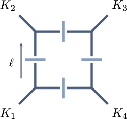
Figure 38: A generic box cut. The momenta $K_{1},K_{2},K_{3},K_{4}$ are assumed to be massive. The loop momentum $\ell$ is defined to be flowing from the $K_{4}$ and into the $K_{1}$ corner.

We define the flattened momenta $K_{1}^{\flat}$, $K_{2}^{\flat}$ as

$$K_{1}^{\flat}=\frac{\gamma^{2}K_{1}-\gamma K_{1}^{2}K_{2}}{\gamma^{2}-K_{1}^{2}K_{2}^{2}},\quad K_{2}^{\flat}=\frac{\gamma^{2}K_{4}-\gamma K_{2}^{2}K_{1}}{\gamma^{2}-K_{1}^{2}K_{2}^{2}}\,.$$ (258)

Here, $\gamma$ is defined by requiring $K_{1}^{\flat}$ and $K_{2}^{\flat}$ to be massless,

$$(K_{1}^{\flat})^{2} =\frac{\gamma^{4}K_{1}^{2}+\gamma^{2}(K_{1}^{2})^{2}K_{2}^{2}-2\gamma^{3}K_{1}^{2}(K_{1}\cdot K_{2})}{(\gamma^{2}-K_{1}^{2}K_{2}^{2})^{2}}=0$$ (259)

$$\Leftrightarrow\gamma^{2}K_{1}^{2}+K_{1}^{2}K_{2}^{2}-2\gamma(K_{1}\cdot K_{2})=0$$ (260)

$$\Rightarrow\gamma=(K_{1}\cdot K_{2})\pm\sqrt{(K_{1}\cdot K_{2})^{2}-K_{1}^{2}K_{2}^{2}}.$$ (261)

In case that either $K_{1}^{2}=0\$ or $K_{2}^{2}=0$, the sign is chosen such that $\gamma$ is non-zero. Additionally, we have

$$\gamma=(K_{1}^{\flat}+K_{2}^{\flat})^{2}=2(K_{1}^{\flat}\cdot K_{2}^{\flat})$$ (262)

and we can re-express $K_{1}$, $K_{2}$ in terms of the flattened momenta via

$$K_{1}=K_{1}^{\flat}+\frac{K_{1}^{2}}{\gamma}K_{2}^{\flat},\quad K_{2}=K_{2}^{\flat}+\frac{K_{2}^{2}}{\gamma}K_{1}^{\flat}.$$ (263)

We use the following representation [29, 30],

$$\overline{\ell}^{\mu}=cK_{2}^{\flat\mu}+dK_{1}^{\flat\mu}+\frac{1}{2}\left(t\mathinner{\langle{K_{2}^{\flat}|\gamma^{\mu}|K_{1}^{\flat}}]}+b\mathinner{\langle{K_{1}^{\flat}|\gamma^{\mu}|K_{2}^{\flat}}]}\right).$$ (264)

The on-shell condition $\ell^{2}=0$ translates into

$$b=\frac{cd\gamma-\mu^{2}}{t\gamma}.$$

Furthermore, the on-shell conditions $(\ell-K_{2})^{2}=0$ and $(\ell+K_{1})^{2}=0$ fix the parameters $c$ and $d$ to be

$$c=-\frac{K_{1}^{2}(\gamma+K_{2}^{2})}{\gamma^{2}-K_{2}^{2}K_{1}^{2}},\quad d=\frac{K_{2}^{2}(\gamma+K_{1}^{2})}{\gamma^{2}-K_{2}^{2}K_{1}^{2}}.$$ (265)

The last on-shell condition $(\ell-K_{2}-K_{3})^{2}=0$ provides a quadratic relation for $t$, with solutions,

$$t^{\pm}=\frac{\Delta\pm\sqrt{\Delta^{2}-4\frac{cd\gamma-\mu^{2}}{\gamma}\text{tr}_{-}(K_{2}^{\flat}K_{3}K_{1}^{\flat}K_{3})}}{2\mathinner{\langle{K_{2}^{\flat}|K_{3}|K_{1}^{\flat}}]}},\quad\Delta=-(2K_{3}\cdot(K_{2}+cK_{2}^{\flat}+dK_{1}^{\flat})+K_{3}^{2})$$ (266)

For rational terms we only require the leading coefficient in the large $\mu^{2}$ expansion. In computations it is therefore sufficient to use the leading behavior of the parameterized loop momentum. Expanding the solutions $t^{\pm}$ of eq. (266) around large values of $\mu^{2}$, we obtain

$$t^{\pm}=\pm\sqrt{\frac{\mu^{2}}{\gamma}}\frac{\mathinner{\langle{K_{1}^{\flat}|K_{3}|K_{2}^{\flat}}]}}{\sqrt{\mathinner{\langle{K_{2}^{\flat}|K_{3}K_{1}^{\flat}K_{3}|K_{2}^{\flat}}]}}}+\mathcal{O}\left[\left(\tfrac{1}{\sqrt{\mu^{2}}}\right)^{0}\right]$$ (267)

In the normalization of amplitudes and Feynman integrals of eqs.(223) and (224), the box $\mu^{4}$ coefficient is given by

$$\operatorname{\mathrm{C}}^{(1)}_{{\mathrm{Box}},[4]}=\frac{1}{2}\sum_{t=t^{\pm}}\operatorname{Inf}_{\mu^{2}}\left.\left[A_{1}^{(0)}A_{2}^{(0)}A_{3}^{(0)}A_{4}^{(0)}\right]\right\rvert_{\mu^{4}}$$ (268)

The operation $\operatorname{Inf}_{x}[f(x)]$ is defined using the expansion of $f(x)$ for large values of $x$ as,

$$f(x)=\operatorname{Inf}_{x}[f(x)]+\mathcal{O}\left[\left(\tfrac{1}{x}\right)\right].$$ (269)

For the following discussion we also define

$$\operatorname{Inf}_{x_{1}x_{2}\mathellipsis x_{n}}[f(x)]\equiv\operatorname{Inf}_{x_{1}}\circ\operatorname{Inf}_{x_{2}}\circ\mathellipsis\circ\operatorname{Inf}_{x_{n}}[f(x)].$$ (270)

F.2 Triangles

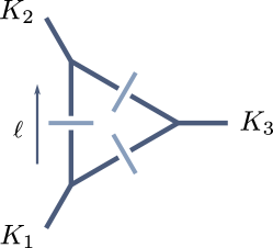
Figure 39: A generic triangle cut. The momenta $K_{1},K_{2},K_{3}$ are generally massive. The loop momentum $\ell$ is defined to flow out of the $K_{3}$ and into the $K_{1}$ corner.

We now turn to the computation of triangle-integral coefficients. We again choose a generic representative with all external momenta $K_{1},K_{2},K_{3}$ being massive, with $\ell$ flowing from the $K_{1}$ to the $K_{2}$ vertex. This configuration is shown in Figure 39.

We reuse the parametrization of the box loop momentum, relaxing the on-shell condition that fixes the $t$ parameter. We again define the massless momenta associated to $K_{1}$ and $K_{2}$,

$$K_{1}^{\flat}=\frac{\gamma^{2}K_{1}-\gamma K_{1}^{2}K_{2}}{\gamma^{2}-K_{1}^{2}K_{2}^{2}},\quad K_{2}^{\flat}=\frac{\gamma^{2}K_{2}-\gamma K_{2}^{2}K_{1}}{\gamma^{2}-K_{1}^{2}K_{2}^{2}},$$ (271)

where

$$\gamma=(K_{1}\cdot K_{2})\pm\sqrt{(K_{1}\cdot K_{2})^{2}-K_{1}^{2}K_{2}^{2}}.$$

Again, when either $K_{1}^{2}$ or $K_{2}^{2}$ vanishes, we choose the sign in front of the square-root such that $\gamma$ is non-zero. The three on-shell conditions $\ell^{2}=0$, $(\ell-K_{2})^{2}=0$ and $(\ell+K_{1})^{2}=0$ are then exactly those of the box case, and are fulfilled by

$$\ell^{\mu}(t)=cK_{2}^{\flat\mu}+dK_{1}^{\flat\mu}+\frac{1}{2}\left(t\mathinner{\langle{K_{2}^{\flat}|\gamma^{\mu}|K_{1}^{\flat}}]}+\frac{cd\gamma-\mu^{2}}{t\gamma}\mathinner{\langle{K_{1}^{\flat}|\gamma^{\mu}|K_{2}^{\flat}}]}\right)$$ (272)

with

$$c=-\frac{K_{1}^{2}(\gamma+K_{2}^{2})}{\gamma^{2}-K_{2}^{2}K_{1}^{2}},\quad d=\frac{K_{2}^{2}(\gamma+K_{1}^{2})}{\gamma^{2}-K_{2}^{2}K_{1}^{2}}.$$ (273)

Unlike the case of the box loop momentum, $t$ is now a remaining degree of freedom that is integrated over.

As in the box case, the on-shell conditions yield two independent solutions. When neither $K_{1}^{2}$ nor $K_{2}^{2}$ vanishes these are given by the two different solutions for $\gamma$. Should one or both of the $K_{i}^{2}$ vanish, we have to choose the sign in $\gamma$ such that it is non-zero. In this case, the second solution can be obtained from the one in eq. (272) via spinor conjugation,

$$\ell^{\ast\mu}(t)=cK_{2}^{\flat\mu}+dK_{1}^{\flat\mu}+\frac{1}{2}\left(t\mathinner{[{K_{2}^{\flat}|\gamma^{\mu}|K_{1}^{\flat}}\rangle}+\frac{cd\gamma-\mu^{2}}{t\gamma}\mathinner{[{K_{1}^{\flat}|\gamma^{\mu}|K_{2}^{\flat}}\rangle}\right)$$ (274)

The fact that we have two solutions for the triangle loop momentum does not mean that imposing an additional on-shell condition for the box parametrization would lead to four solutions. Instead, the resulting solutions for $\ell$ would be degenerate, we would still only end up with two distinct solutions we found in the discussion of box cuts.

In the parameterization of eq. (272) the remaining integrals over positive powers of $t$ vanish, so that we require only the $t^{0}$ contributions. The coefficient of a triangle integral with a $\mu^{2}$ numerator insertion is then [29, 30]

$$\operatorname{\mathrm{C}}^{(1)}_{{\mathrm{Tri}},[2]}=\frac{1}{2}\sum_{\bar{\ell}=\bar{\ell}(t),\bar{\ell}^{\ast}(t)}\operatorname{Inf}_{\mu^{2},t}\left.\left[A_{1}^{(0)}(\ell)A_{2}^{(0)}(\ell)A_{3}^{(0)}(\ell)\right]\right\rvert_{t^{0},\mu^{2}}.$$ (275)

F.3 Bubble

Figure 40: A generic bubble cut. Assuming the massive momentum $K$ to be outgoing, we define the loop momentum $\ell$ to be flowing from the $K$ and into the $-K$ vertex.

Finally we explain how to determine the coefficients of bubble integrals. In this case we have only one external massive momentum $K$, and we define the loop momentum $\ell$ as shown in Figure 40.

As in the triangle case, the derivation of the bubble coefficient will depend on the specific loop momentum parametrization we use to make the on-shell conditions manifest. We would like to choose a parametrization similar to the box and triangle case. However, in this case we cannot define such a parametrization entirely in terms of the external kinematics, as we have only a single momentum $K$. We therefore need to introduce an arbitrary reference momentum $\chi$. Choosing $\chi$ to be lightlike, we define the flattened version of $K$ to be

$$K^{\flat}=K-\frac{K^{2}}{\gamma}\chi,\quad\text{with}\quad\gamma=2(K\cdot\chi)=2(K^{\flat}\cdot\chi).$$ (276)

Similarly to the box and triangle cases, we use the following representation for the four-dimensional part of the loop momentum $\ell$ [29, 30],

$$\bar{\ell}^{\mu}=-K^{\mu}+yK^{\flat\mu}+d\chi^{\mu}+\frac{1}{2}\left(t\mathinner{\langle{K^{\flat}|\gamma^{\mu}|\chi}]}+b\mathinner{\langle{\chi|\gamma^{\mu}|K^{\flat}}]}\right).$$ (277)

The on-shell conditions $\ell^{2}=0$ and $(\ell+K)^{2}=0$ then fix the parameters $b$ and $d$ to be,

$$d=\frac{K^{2}(1-y)}{\gamma},\hskip 20.00003ptb=\frac{\gamma dy-\mu^{2}}{ty}=\frac{y(1-y)K^{2}-\mu^{2}}{t\gamma},$$ (278)

so that

$$\bar{\ell}^{\mu}(t,y)=(y-1)K^{\flat\mu}-y\frac{K^{2}}{\gamma}\chi^{\mu}+\frac{1}{2}\left(t\mathinner{\langle{K^{\flat}|\gamma^{\mu}|\chi}]}+\frac{y(1-y)K^{2}-\mu^{2}}{t\gamma}\mathinner{\langle{\chi|\gamma^{\mu}|K^{\flat}}]}\right)\,.$$ (279)

In contrast to the box and triangle coefficients, there are two sources of contributions to the bubble coefficient. One is the bubble cut itself, where two tree amplitudes are evaluated using the parametrization of eq. (279). We are left with integrals over the two remaining parameters $t$ and $y$. In the chosen parametrization the integrals over powers of $t$ vanish, so that we require only the parts of the cut of order $t^{0}$. The integrals over positive powers of $y$ do not vanish. Power counting in Yang–Mills theory limits the maximal power of $y$ to two. Carrying out the integrals amounts to expanding the cut for large values of $y$, and replacing $y^{0}$, $y^{1}$ and $y^{2}$ with [77, 30]

$$Y_{0}=1,\qquad Y_{1}=-\frac{1}{2},\qquad Y_{2}=\frac{1}{3}\left(1-\frac{\mu^{2}}{s}\right).$$ (280)

The second source of contributions are tensor triangles, which after Passarino–Veltman reduction also contain terms belonging to the bubble basis integrals. Only triangle cuts which have two cuts in common with the bubble cut will contribute. As an example, consider the integral in Figure 41. In addition to the two bubble cut, a third propagator $(\ell+K+K^{\prime})^{2}$ has been cut. To determine the contribution to the bubble coefficient we need to use the same parameterization as for the bubble cut. The additional on-shell condition leads to two solutions for $y$ [77, 30]

$$y^{\pm} =\frac{c_{1}\pm\sqrt{c_{1}^{2}+4c_{0}c_{2}}}{2c_{2}}$$ (281)

where,

$$c_{0} =t\left[\gamma(K^{\prime})^{2}+2(K^{\prime}\cdot\chi)K^{2}\right]+t^{2}\gamma\mathinner{\langle{K^{\flat}|K^{\prime}|\chi}]}-\mu^{2}\mathinner{\langle{\chi|K^{\prime}|K^{\flat}}]}\,,$$ (282)

$$c_{1} =K^{2}\mathinner{\langle{\chi|K^{\prime}|K^{\flat}}]}+t\left[\gamma 2(K^{\prime}\cdot K^{\flat})-K^{2}2(K^{\prime}\cdot\chi)\right]\,,$$

$$c_{2} =K^{2}\mathinner{\langle{\chi|K^{\prime}|K^{\flat}}]}\,.$$

Evaluating the triangle cut at $\bar{\ell}(t,y^{\pm})$, we are left with in integrals over powers of the remaining parameter $t$. Only integrals with $t^{i>0}$ are relevant for the bubble coefficient, as only these are related to tensor integrals. Power counting in Yang–Mills again limits the maximal power which can appear, this time to $i\leq 3$ [30]. In contrast to computation of the triangle coefficient, these integrals no longer vanish, as their vanishing was a special feature of the triangle parameterization of eq. (272). Additionally, we do not require the full integral over the $t^{i}$, but only the bubble contributions after Passarino–Veltman reduction. These were determined in ref. [77]. To obtain the contribution of the tensor triangle to the bubble coefficient, we can follow a simple recipe: we expand the triangle cut for large values of $t$, remove the constant term, and replace $t$, $t^{2}$ and $t^{3}$ with [30, 77],

$$T_{1} =-\frac{K^{2}\mathinner{\langle{\chi|K^{\prime}|K^{\flat}}]}}{2\gamma\left[(K\cdot K^{\prime})^{2}-K^{2}K^{\prime 2}\right]}\,,$$ (283)

$$T_{2} =\frac{3(K^{2})^{2}\mathinner{\langle{\chi|K^{\prime}|K^{\flat}}]}^{2}}{8\gamma^{2}\left[(K\cdot K^{\prime})^{2}-(K^{2})K^{2}\right]^{2}}\left[(K\cdot K^{\prime})+K^{\prime 2}\right]\,,$$

$$T_{3} =-\frac{(K^{2})^{3}\mathinner{\langle{\chi|K^{\prime}|K^{\flat}}]}^{3}}{48\gamma^{3}\left[(K\cdot K^{\prime})^{2}-K^{2}K^{\prime 2}\right]^{3}}$$

$$\hphantom{=}\times\left((K\cdot K^{\prime})^{2}\left(11+16\frac{\mu^{2}}{K^{2}}\right)+30(K\cdot K^{\prime})K^{\prime 2}+K^{\prime 2}\left(4K^{2}+15K^{\prime 2}-16\mu^{2}\right)\right)\,.$$

Summing over all triangle cuts compatible with the bubble cut, we obtain the full bubble coefficient via,

$$\operatorname{\mathrm{C}}^{(1)}_{{\mathrm{Bub}},[2]} =\operatorname{Inf}_{\mu^{2},t,y}\left.\left[A_{1}^{(0)}A_{2}^{(0)}\right]\right\rvert_{\mu^{2},t^{0},y^{i}\to Y_{i}}+\frac{1}{2}\sum_{\begin{subarray}{c}\text{triangle}\\ \text{cuts}\end{subarray}}\sum_{y^{\pm}}\operatorname{Inf}_{\mu^{2},t}\left.\left[A_{1}^{(0)}A_{2}^{(0)}A_{3}^{(0)}\right]\right\rvert_{\mu^{2},t^{i}\to T_{i}}.$$ (284)

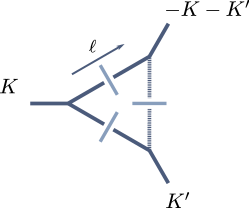
Figure 41: An example of a triangle cut contributing to the bubble coefficient. The momentum $K$ and the solid lines are those belonging to the original bubble. The momentum $K^{\prime}$ and dashed lines are those of the additional on-shell condition.

References

- [1] M. L. Mangano and S. J. Parke, Phys. Rept. 200 (1991), 301-367 doi:10.1016/0370-1573(91)90091-Y [hep-th/0509223].
- [2] R. K. Ellis and J. C. Sexton, Nucl. Phys. B 269, 445-484 (1986) doi:10.1016/0550-3213(86)90232-4
- [3] Z. Bern, L. J. Dixon and D. A. Kosower, Phys. Rev. Lett. 70, 2677-2680 (1993) doi:10.1103/PhysRevLett.70.2677 [arXiv:hep-ph/9302280 [hep-ph]].
- [4] Z. Bern, G. Chalmers, L. J. Dixon and D. A. Kosower, Phys. Rev. Lett. 72, 2134-2137 (1994) doi:10.1103/PhysRevLett.72.2134 [arXiv:hep-ph/9312333 [hep-ph]].
- [5] G. Mahlon, T. M. Yan and C. Dunn, Phys. Rev. D 48, 1337-1374 (1993) doi:10.1103/PhysRevD.48.1337 [arXiv:hep-ph/9210212 [hep-ph]].
- [6] G. Mahlon, doi:10.1103/PhysRevD.49.4438 [arXiv:hep-ph/9312276 [hep-ph]].
- [7] Z. Bern, L. J. Dixon, D. C. Dunbar and D. A. Kosower, Phys. Lett. B 394, 105-115 (1997) [arXiv:hep-th/9611127 [hep-th]].
- [8] R. Britto, G. R. Jehu and A. Orta, JHEP 04, 276 (2021) doi:10.1007/JHEP04(2021)276 [arXiv:2011.13821 [hep-th]].
- [9] D. Chicherin and J. M. Henn, [arXiv:2202.05596 [hep-th]]; D. Chicherin and J. Henn, [arXiv:2204.00329 [hep-th]].
- [10] Z. Bern, L. J. Dixon and D. A. Kosower, JHEP 01, 027 (2000) [arXiv:hep-ph/0001001 [hep-ph]].
- [11] S. Badger, H. Frellesvig and Y. Zhang, JHEP 12, 045 (2013) [arXiv:1310.1051 [hep-ph]].
- [12] S. Badger, G. Mogull, A. Ochirov and D. O’Connell, JHEP 10, 064 (2015) doi:10.1007/JHEP10(2015)064 [arXiv:1507.08797 [hep-ph]].
- [13] T. Gehrmann, J. M. Henn and N. A. Lo Presti, Phys. Rev. Lett. 116, no.6, 062001 (2016) [erratum: Phys. Rev. Lett. 116, no.18, 189903 (2016)] doi:10.1103/PhysRevLett.116.062001 [arXiv:1511.05409 [hep-ph]].
- [14] S. Abreu, F. Febres Cordero, H. Ita, B. Page and M. Zeng, Phys. Rev. D 97, no.11, 116014 (2018) doi:10.1103/PhysRevD.97.116014 [arXiv:1712.03946 [hep-ph]].
- [15] S. Badger, D. Chicherin, T. Gehrmann, G. Heinrich, J. M. Henn, T. Peraro, P. Wasser, Y. Zhang and S. Zoia, Phys. Rev. Lett. 123, no.7, 071601 (2019) doi:10.1103/PhysRevLett.123.071601 [arXiv:1905.03733 [hep-ph]].
- [16] Q. Jin and H. Luo, [arXiv:1910.05889 [hep-ph]].
- [17] F. Caola, A. Chakraborty, G. Gambuti, A. von Manteuffel and L. Tancredi, Phys. Rev. Lett. 128, no.21, 212001 (2022) doi:10.1103/PhysRevLett.128.212001 [arXiv:2112.11097 [hep-ph]].
- [18] D. C. Dunbar, G. R. Jehu and W. B. Perkins, Phys. Rev. D 93, no.12, 125006 (2016) doi:10.1103/PhysRevD.93.125006 [arXiv:1604.06631 [hep-th]].
- [19] D. C. Dunbar, G. R. Jehu and W. B. Perkins, Phys. Rev. Lett. 117, no.6, 061602 (2016) doi:10.1103/PhysRevLett.117.061602 [arXiv:1605.06351 [hep-th]].
- [20] D. C. Dunbar and W. B. Perkins, Phys. Rev. D 93, no.8, 085029 (2016) doi:10.1103/PhysRevD.93.085029 [arXiv:1603.07514 [hep-th]].
- [21] D. C. Dunbar, G. R. Jehu and W. B. Perkins, Phys. Rev. D 93 (2016) no.12, 125006 doi:10.1103/PhysRevD.93.125006 [arXiv:1604.06631 [hep-th]].
- [22] D. C. Dunbar, J. H. Godwin, G. R. Jehu and W. B. Perkins, Phys. Rev. D 96, no.11, 116013 (2017) doi:10.1103/PhysRevD.96.116013 [arXiv:1710.10071 [hep-th]].
- [23] D. C. Dunbar, J. H. Godwin, G. R. Jehu and W. B. Perkins, PoS RADCOR2017, 026 (2017) doi:10.22323/1.290.0026 [arXiv:1712.05312 [hep-ph]].
- [24] A. R. Dalgleish, D. C. Dunbar, W. B. Perkins and J. M. W. Strong, Phys. Rev. D 101, no.7, 076024 (2020) doi:10.1103/PhysRevD.101.076024 [arXiv:2003.00897 [hep-ph]].
- [25] D. C. Dunbar, J. H. Godwin, W. B. Perkins and J. M. W. Strong, Phys. Rev. D 101, no.1, 016009 (2020) doi:10.1103/PhysRevD.101.016009 [arXiv:1911.06547 [hep-ph]].
- [26] S. Badger, G. Mogull and T. Peraro, JHEP 08, 063 (2016) [arXiv:1606.02244 [hep-ph]].
- [27] D. A. Kosower and K. J. Larsen, Phys. Rev. D 85:045017 (2012) doi:10.1103/PhysRevD.85.045017 [arXiv:1108.1180].
- [28] R. Britto, F. Cachazo and B. Feng, Nucl. Phys. B 725 (2005), 275-305 doi:10.1016/j.nuclphysb.2005.07.014 [arXiv:hep-th/0412103 [hep-th]].
- [29] D. Forde, Phys. Rev. D 75, 125019 (2007) doi:10.1103/PhysRevD.75.125019 [arXiv:0704.1835 [hep-ph]].
- [30] S. D. Badger, JHEP 01, 049 (2009) [arXiv:0806.4600 [hep-ph]].
- [31] G. Ossola, C. G. Papadopoulos and R. Pittau, Nucl. Phys. B 763, 147-169 (2007) doi:10.1016/j.nuclphysb.2006.11.012 [arXiv:hep-ph/0609007 [hep-ph]].
-
[32]
D. C. Dunbar and W. B. Perkins,
Phys. Rev. D 93:085029 (2016)
[arXiv:1603.07514];
D. C. Dunbar, G. R. Jehu and W. B. Perkins, Phys. Rev. Lett. 117:061602 (2016) [arXiv:1605.06351];
D. C. Dunbar, J. H. Godwin, G. R. Jehu and W. B. Perkins, Phys. Rev. D 96:116013 (2017) doi:10.1103/PhysRevD.96.116013 [arXiv:1710.10071]. - [33] D. C. Dunbar, W. B. Perkins and J. M. W. Strong, Phys. Rev. D 101, no.7, 076001 (2020) doi:10.1103/PhysRevD.101.076001 [arXiv:2001.11347 [hep-ph]].
-
[34]
D. C. Dunbar, J. H. Godwin, W. B. Perkins and J. M. W. Strong,
Phys. Rev. D 101:016009 (2020)
[arXiv:1911.06547];
A. R. Dalgleish, D. C. Dunbar, W. B. Perkins and J. M. W. Strong, Phys. Rev. D 101:076024 (2020) [arXiv:2003.00897]. - [35] R. Britto, F. Cachazo, B. Feng and E. Witten, Phys. Rev. Lett. 94, 181602 (2005) doi:10.1103/PhysRevLett.94.181602 [arXiv:hep-th/0501052 [hep-th]].
- [36] Z. Bern and D. A. Kosower, Nucl. Phys. B 362, 389-448 (1991) doi:10.1016/0550-3213(91)90567-H
- [37] W. T. Giele and E. W. N. Glover, Phys. Rev. D 46, 1980-2010 (1992) doi:10.1103/PhysRevD.46.1980
-
[38]
Z. Bern, L. J. Dixon, D. C. Dunbar and D. A. Kosower,
Nucl. Phys. B 425, 217-260 (1994)
doi:10.1016/0550-3213(94)90179-1
[arXiv:hep-ph/9403226 [hep-ph]];
Z. Bern, L. J. Dixon, D. C. Dunbar and D. A. Kosower, Nucl. Phys. B 435, 59-101 (1995) doi:10.1016/0550-3213(94)00488-Z [arXiv:hep-ph/9409265 [hep-ph]]. - [39] Z. Kunszt, A. Signer and Z. Trocsanyi, Nucl. Phys. B 420, 550-564 (1994) doi:10.1016/0550-3213(94)90077-9 [arXiv:hep-ph/9401294 [hep-ph]].
- [40] S. Catani and M. H. Seymour, Nucl. Phys. B 485, 291-419 (1997) [erratum: Nucl. Phys. B 510, 503-504 (1998)] doi:10.1016/S0550-3213(96)00589-5 [arXiv:hep-ph/9605323 [hep-ph]].
- [41] R. E. Cutkosky, J. Math. Phys. 1, 429-433 (1960) doi:10.1063/1.1703676
- [42] E. W. N. Glover, C. Oleari and M. E. Tejeda-Yeomans, Nucl. Phys B 605, 467-485 (2001) doi:10.1016/S0550-3213(01)00210-3 [arXiv:hep-ph/0102201 [hep-ph]].
- [43] Z. Bern, A. De Freitas and L. J. Dixon, JHEP 03, 018 (2002) doi:10.1088/1126-6708/2002/03/018 [arXiv:hep-ph/0201161 [hep-ph]].
- [44] S. Badger, G. Mogull, A. Ochirov and D. O’Connell, JHEP 10, 064 (2015) [arXiv:1507.08797 [hep-ph]].
- [45] S. Catani, Phys. Lett. B 427, 161-171 (1998) doi:10.1016/S0370-2693(98)00332-3 [arXiv:hep-ph/9802439 [hep-ph]].
- [46] W. T. Giele, Z. Kunszt and K. Melnikov, JHEP 04, 049 (2008) [arXiv:0801.2237 [hep-ph]].
- [47] S. Badger, C. Brønnum-Hansen, H. B. Hartanto and T. Peraro, JHEP 01, 186 (2019) doi:10.1007/JHEP01(2019)186 [arXiv:1811.11699 [hep-ph]].
- [48] S. Abreu, F. Febres Cordero, H. Ita, M. Jaquier, B. Page and M. Zeng, Phys. Rev. Lett. 119, no.14, 142001 (2017) doi:10.1103/PhysRevLett.119.142001 [arXiv:1703.05273 [hep-ph]].
- [49] S. Abreu, F. Febres Cordero, H. Ita, B. Page and V. Sotnikov, JHEP 11, 116 (2018) doi:10.1007/JHEP11(2018)116 [arXiv:1809.09067 [hep-ph]].
- [50] S. Abreu, J. Dormans, F. Febres Cordero, H. Ita and B. Page, Phys. Rev. Lett. 122, no.8, 082002 (2019) doi:10.1103/PhysRevLett.122.082002 [arXiv:1812.04586 [hep-ph]].
- [51] S. Abreu, L. J. Dixon, E. Herrmann, B. Page and M. Zeng, JHEP 03, 123 (2019) doi:10.1007/JHEP03(2019)123 [arXiv:1901.08563 [hep-th]].
- [52] S. Abreu, J. Dormans, F. Febres Cordero, H. Ita, B. Page and V. Sotnikov, JHEP 05, 084 (2019) doi:10.1007/JHEP05(2019)084 [arXiv:1904.00945 [hep-ph]].
- [53] S. Abreu, F. Febres Cordero, H. Ita, M. Jaquier, B. Page, M. S. Ruf and V. Sotnikov, Phys. Rev. Lett. 124, no.21, 211601 (2020) doi:10.1103/PhysRevLett.124.211601 [arXiv:2002.12374 [hep-th]].
- [54] S. Abreu, B. Page, E. Pascual and V. Sotnikov, JHEP 01, 078 (2021) doi:10.1007/JHEP01(2021)078 [arXiv:2010.15834 [hep-ph]].
- [55] S. Abreu, F. Febres Cordero, H. Ita, B. Page and V. Sotnikov, JHEP 07, 095 (2021) doi:10.1007/JHEP07(2021)095 [arXiv:2102.13609 [hep-ph]].
- [56] M. Accettulli Huber, A. Brandhuber, S. De Angelis and G. Travaglini, Phys. Rev. D 101, no.2, 026004 (2020) doi:10.1103/PhysRevD.101.026004 [arXiv:1910.04772 [hep-th]].
- [57] T. Kaluza, Sitzungsber. Preuss. Akad. Wiss. Berlin (Math. Phys. ) 1921, 966-972 (1921) doi:10.1142/S0218271818700017 [arXiv:1803.08616 [physics.hist-ph]]; O. Klein, Z. Phys. 37, 895-906 (1926) doi:10.1007/BF01397481
- [58] J. E. Paton and H. M. Chan, Nucl. Phys. B 10, 516-520 (1969) doi:10.1016/0550-3213(69)90038-8
- [59] C. Cheung and D. O’Connell, JHEP 07, 075 (2009) doi:10.1088/1126-6708/2009/07/075 [arXiv:0902.0981 [hep-th]].
- [60] Z. Bern, J. J. Carrasco, T. Dennen, Y. t. Huang and H. Ita, Phys. Rev. D 83, 085022 (2011) doi:10.1103/PhysRevD.83.085022 [arXiv:1010.0494 [hep-th]].
- [61] S. D. Badger, E. W. N. Glover, V. V. Khoze and P. Svrcek, JHEP 07, 025 (2005) doi:10.1088/1126-6708/2005/07/025 [arXiv:hep-th/0504159 [hep-th]].
- [62] D. Forde and D. A. Kosower, Phys. Rev D 73, 065007 (2006) doi:10.1103/PhysRevD.73.065007 [arXiv:hep-th/0507292 [hep-th]].
- [63] G. Rodrigo, JHEP 09, 079 (2005) doi:10.1088/1126-6708/2005/09/079 [arXiv:hep-ph/0508138 [hep-ph]].
- [64] C. Schwinn and S. Weinzierl, JHEP 03, 030 (2006) doi:10.1088/1126-6708/2006/03/030 [arXiv:hep-th/0602012 [hep-th]].
- [65] P. Ferrario, G. Rodrigo and P. Talavera, Phys. Rev. Lett. 96, 182001 (2006) [arXiv:hep-th/0602043 [hep-th]].
- [66] J. J. M. Carrasco and I. A. Vazquez-Holm, Phys. Rev. D 103, no.4, 045002 (2021) doi:10.1103/PhysRevD.103.045002 [arXiv:2010.13435 [hep-th]].
- [67] R. Britto, F. Cachazo, B. Feng and E. Witten, Phys. Rev. Lett. 94, 181602 (2005) doi:10.1103/PhysRevLett.94.181602 [arXiv:hep-th/0501052 [hep-th]].
- [68] C. Schwinn and S. Weinzierl, JHEP 04, 072 (2007) doi:10.1088/1126-6708/2007/04/072 [arXiv:hep-ph/0703021 [hep-ph]].
- [69] D. A. Kosower, Phys. Rev D 71, 045007 (2005) doi:10.1103/PhysRevD.71.045007 [arXiv:hep-th/0406175 [hep-th]].
- [70] A. C. Edison and S. G. Naculich, Nucl. Phys B 858, 488-501 (2012) doi:10.1016/j.nuclphysb.2012.01.019 [arXiv:1111.3821 [hep-th]].
- [71] J. M. Henn and J. C. Plefka, Lect. Notes Phys. 883, pp.1-195 (2014) doi:10.1007/978-3-642-54022-6
- [72] Z. Bern, L. J. Dixon and D. A. Kosower, Phys. Lett B 302, 299-308 (1993) [erratum: Phys. Lett B 318, 649 (1993)] doi:10.1016/0370-2693(93)90400-C [arXiv:hep-ph/9212308 [hep-ph]].
- [73] Z. Bern, L. J. Dixon, M. Perelstein and J. S. Rozowsky, Nucl. Phys. B 546, 423-479 (1999) doi:10.1016/S0550-3213(99)00029-2 [arXiv:hep-th/9811140 [hep-th]].
- [74] R. Kleiss and H. Kuijf, Nucl. Phys B 312, 616-644 (1989) doi:10.1016/0550-3213(89)90574-9
- [75] A. Hodges, JHEP 05, 135 (2013) doi:10.1007/JHEP05(2013)135 [arXiv:0905.1473 [hep-th]].
- [76] L. Budge, J. M. Campbell, G. De Laurentis, R. K. Ellis and S. Seth, JHEP 05, 079 (2020) doi:10.1007/JHEP05(2020)079 [arXiv:2002.04018 [hep-ph]].
- [77] W. B. Kilgore, [arXiv:0711.5015 [hep-ph]].