Cyclical Kernel Adaptive Metropolis

Abstract

We propose cKAM, cyclical Kernel Adaptive Metropolis, which incorporates a cyclical stepsize scheme to allow control for exploration and sampling. We show that on a crafted bimodal distribution, existing Adaptive Metropolis type algorithms would fail to converge to the true posterior distribution. We point out that this is because adaptive samplers estimates the local/global covariance structure using past history of the chain, which will lead to adaptive algorithms be trapped in a local mode. We demonstrate that cKAM encourages exploration of the posterior distribution and allows the sampler to escape from a local mode, while maintaining the high performance of adaptive methods.

1 Introduction

Bayesian inference is know for its ability for probabilistic modeling for data. Markov Chain Monte Carlo (MCMC) is a class of sampling methods where we obtain a sequence of samples from a probability distribution. Given a dataset $\mathcal{D}=\left\{x_{i}\right\}_{i=1}^{N}$ and a model parametrized by $\theta$, MCMC samplers construct a Markov chain with the desired distribution as its stationary distribution, it is guaranteed to converge to the true distribution

$$\uppi(\theta)\propto\exp{\Big{(}\log{p(\mathcal{D}|\theta)}+\log{p(\theta)}\Big{)}},$$

The choice of proposal $q(\cdot|\theta_{t})$ for constructing the Markov chain is crucial for the performance of an MCMC sampler. To increase the efficiency of a sampler, methods for adapting the covariance structure of posterior base on the running history of the chain such as Adaptive-Metropolis (AM) (Haario et al., 2001), global adaptive scaling and other more sophisticated schemes (Andrieu & Thoms, 2008) have been introduced, and the mixing and ergodicity of this type of algorithms has been well studied (Roberts & Rosenthal, 2007) (Atchadé et al., 2011). However, these samplers are only useful for distributions that show high anisotropy. To allow adaptation in strongly non-linear target distributions where the directions of variation depends the current position $\theta_{t}$, Kernel Adaptive Metropolis-Hastings (KAM) is proposed (Sejdinovic et al., 2014). KAM adapts to the local covariance structure, since the proposed next state $\theta^{\prime}$ is the pre-image of a sample in the Reproducing Kernel Hilbert Space (RKHS) with a Gaussian Measure.

In this work, we propose a variant of KAM, the cyclic Kernel Adaptive Metropolis (cKAM), that shows local adaptation, while using cyclic stepsize scheme to control Exploration and Sampling. Compare with KAM, cKAM only recomputes kernel gradient matrix $M_{\mathbf{z},\theta}$ during the Exploration, thus greatly reduces the cost of making a proposal.

Through experimenting with a synthetic two-dimensional bimodal target distribution, we demonstrate that cKAM’s stepsize scheme allows us to jump between different modes and converges to the correct distribution, whereas previous adaptive samplers failed in finding all the modes. We also showed that cKAM is able to retain similar performance as KAM in following non-linear targets: 1) 2d Gaussian Mixtures target distribution and 2) 32-dimensional Gaussian Mixtures target distribution.

2 Kernel Adaptive Metropolis-Hastings

We restates algorithm formulation for KAM in Algorithm 1, clearly identify adaptation for both stepsize and covariance. KAM adapts to the local covariance structure, by proposing the kernel form of next position, $f=k(\cdot,\theta^{\prime})$, in a reproducing kernel Hilbert space (RKHS) $\mathcal{H}_{k}$ with a Gaussian measure. The “density” form of this measure can be denoted as $\mathcal{N}(f;k(\cdot,\theta_{t}),\nu^{2}C_{\mathbf{z}})$ where $C_{\mathbf{z}}$ is the empirical covariance operator on a random subsample of chain history $\mathbf{z}$. The pre-image $\theta^{\prime}$ of $f$ is found by taking a gradient descent step w.r.t. $\theta_{t}$, and this move can be analytically integrated out, as in line 9, Algorithm 1.

We note that the KAM proposal is different from 1) Random-Walk (RW) proposal where $q(\cdot|\theta_{t})=\mathcal{N}({\cdot|\theta_{t},\Sigma})$ (Brooks et al., 2011) and 2) gradient-based proposals using Hamiltonian dynamics (Neal, 2011) or Langevin dynamics(Roberts & Stramer, 2002). Although KAM proposal doesn’t use gradient information of the posterior as it maps past chain history into RKHS space, it still captures some level of neighboring posterior geometry; therefore KAM’s proposal lies in between RW and gradient-based proposals.

There are two computational costs associated with making a proposal in RKHS space: 1) computing the kernel gradient matrices for both $M_{\mathbf{z},\theta^{\prime}}^{T}$ and $M_{\mathbf{z},\theta_{t}}^{T}$ which requires computing the gradient of the kernel function for $m$ subsamples of chain history; and 2) computing the density of two multivariate normal distributions with non-diagonal covariance matrices. We aim to amortize these cost with the design of a new algorithm.

Algorithm 1 Kernel Adaptive Metropolis-Hastings (Sejdinovic et al., 2014)

  Input: initial state $\theta_{0}\in\Theta$, subsample size $m$, initial stepsize $\nu$, noise $\gamma$, stepsize adaptation $\epsilon$, total iterations $T$, burin $B$, adaptation probabilities $\{p_{t}\}_{t=0}^{\infty}$, kernel gradient $\nabla_{\theta_{t}}k(\theta_{t},\theta^{\prime})$, optimal acceptance $\alpha^{*}$

  Let $samples=\{\}$

  for t in $0:T$ do

      $\triangleright$ Propose next state by finding pre-image of a RKHS sample

     Let $\mathcal{M}={\min(m,t+1)}$

     with probability $p_{t}$, random subsample $\mathbf{z}=\{z_{i}\}_{i=0}^{\mathcal{M}-1}$ from history $\{\theta_{i}\}_{i=0}^{t-1}$

     Let $H=I-\frac{1}{\mathcal{M}}\mathbf{1}_{\mathcal{M}\times\mathcal{M}}$ the centering matrix in $\mathbb{R}^{\mathcal{M}\times\mathcal{M}}$

     Let $M_{\mathbf{z},\theta_{t}}=2[\nabla_{\theta_{t}}k(\theta_{t},z_{0}),...,\nabla_{\theta_{t}}k(\theta_{t},z_{m-1})]$ the kernel gradient matrix in $\mathbb{R}^{d\times m}$

     Propose next state $\theta^{\prime}$ through sampling from $\mathcal{N}(\theta_{t},\gamma^{2}I+\nu^{2}M_{\mathbf{z},\theta_{t}}HM_{\mathbf{z},\theta_{t}}^{T})$

      $\triangleright$ Compute acceptance ratio $\alpha_{t}$

     Compute multivariate normal PDF, $q_{\mathbf{z}}(\theta^{\prime}|\theta_{t})=\mathcal{N}(\theta_{t},\gamma^{2}I+\nu^{2}M_{\mathbf{z},\theta_{t}}HM_{\mathbf{z},\theta_{t}}^{T})$ and $q_{\mathbf{z}}(\theta_{t}|\theta^{\prime})=\mathcal{N}(\theta^{\prime},\gamma^{2}I+\nu^{2}M_{\mathbf{z},\theta^{\prime}}HM_{\mathbf{z},\theta^{\prime}}^{T})$.

     Let $\alpha_{t}=\min\left\{1,\frac{\uppi(\theta^{\prime})q_{\mathbf{z}}(\theta_{t}|\theta^{\prime})}{\uppi(\theta_{t})q_{\mathbf{z}}(\theta^{\prime}|\theta_{t})}\right\}$

      $\triangleright$ Accept or reject the samples

     With probability $\alpha_{t}$, $\theta_{t+1}=\theta^{\prime}$

     $samples=\{\theta_{t+1},samples\}$ If $t>B$

      $\triangleright$ Adapting the stepsize $\nu$

     $\nu=\exp(\log(\nu)+\eta[\alpha_{t}-\alpha^{*}])$ where $\eta=\frac{1}{(1+\epsilon)^{t}}$

  end for

2.1 Local vs. Global Covariance Estimate

Standard AM and its variants estimate the empirical covariance matrix (Atchadé et al., 2011; Andrieu & Thoms, 2008; Chen et al., 2016) base on the chain history of past samples $\{\theta_{i}\}_{i=0}^{t-1}$. However, these algorithms treat each sample equally, and updates the empirical covariance matrix regardless local landscape of posterior, therefore estimates a global covariance (Roberts & Rosenthal, 2007).

KAM can adapt to the local covariance structure, because past samples are treated differently. KAM proposal computes the kernel gradient matrix $M_{\mathbf{z},\theta}$ on kernel functions $k(\theta,z_{i})$, which will give larger values for $z_{i}$ closer to current position $\theta$ as long as the kernel is not a linear kernel. This proposal make better use of information encoded in past samples that are neighboring to current position even though samples are proposed from a Gaussian distribution.

2.2 Kernel Functions and Their Gradients

Here we summarize kernels used in the original KAM paper, and their derivatives, which will be used to compute corresponding kernel gradient matrices.

• Linear Kernel. The kernel function is $k(\theta,z)=\theta^{T}z$, its gradient w.r.t. $\theta$ is $\nabla_{\theta}k(\theta,z)=z$.

• Guassian (RBF) Kernel. The kernel function is $k_{l}(\theta,z)=\exp{\left(-||\theta-z||_{2}^{2}/2l^{2}\right)}$, its gradient w.r.t. $\theta$ is $\nabla_{\theta}k_{l}(\theta,z)=k_{l}(\theta,z)(z-x)/l^{2}$.

• Matérn Kernel. The kernel function is $k_{v,l}(\theta,z)=\frac{1}{\Gamma(v)2^{v-1}}\left(\frac{\sqrt{2v}}{l}||\theta-z||_{2}\right)^{v}K_{v}\left(\frac{\sqrt{2v}}{l}||\theta-z||_{2}\right),$ where $K_{v}(\cdot)$ is a modified Bessel function of the second kind for real order $v$, and $\Gamma(\cdot)$ is the gamma function. Its gradient w.r.t. $\theta$ is $\nabla_{\theta}k_{v,l}(\theta,z)=\frac{v}{l^{2}(v-1)}k_{v-1,l}(\theta,z)(z-x)$

2.3 cKAM and cyclical stepsize

While KAM can adapt to the local covariance of a strongly non-linear target distribution, this behavior will hinder the sampler to properly explore a multimodal distribution. We want to design an algorithm that 1) unitizes KAM’s ability to adapt to local covariance structure, while avoiding the large cost of making proposal in every iteration of the chain and 2) allows exploration to various modes of the target posterior (Pompe et al., 2020).

Inspired by recent success of cSG-MCMC (Zhang et al., 2020c) in using cyclical step size for Bayesian Deep Learning, here we propose cyclical Kernel Adaptive Metropolis, cKAM, that splits the normal Burnin and Sampling phases in normal MCMC methods into cycles of Exploration and Sampling.

Algorithm 2 Cyclical Kernel Adaptive Metropolis

  Input: initial state $\theta_{0}\in\Theta$, subsample size $m$, initial stepsize $\nu$, noise $\gamma$, stepsize adaptation $\epsilon$, total iterations $T$, adaptation probabilities $\{p_{t}\}_{t=0}^{\infty}$, kernel gradient $\nabla_{\theta_{t}}k(\theta_{t},\theta^{\prime})$, optimal acceptance $\alpha^{*}$,

  new hyperparameters: proporation of exploration $\beta$, number of cycles $M$

  Let $samples=\{\}$

  for m in $0:M-1$ do

      $\triangleright$ Exploration phase

     for  $0\leq\frac{\text{mod}{(t-1,\lceil T/M\rceil)}}{\lceil T/M\rceil}\leq\beta$ do

        Same behavior as in KAM, except 1) no samples are added to $samples$, 2) the random subsample $\mathbf{z}$ is only selected from chain history of current cycle

     end for

      $\triangleright$ Transition to Sampling phase, $\lceil\frac{\text{mod}{(t-1,\lceil T/M\rceil)}}{\lceil T/M\rceil}\rceil=\beta$, $t=t_{exp}$

     Let $\nu_{0}=({2\nu_{exp}})/({\cos(\beta\uppi)+1})$

     Let $\Sigma=(\frac{\gamma}{\nu_{exp}})^{2}I+M_{\mathbf{z},\theta_{t}}HM_{\mathbf{z},\theta_{t}}^{T}$

      $\triangleright$ Sampling phase

     for  $\beta<\frac{\text{mod}{(t-1,\lceil T/M\rceil)}}{\lceil T/M\rceil}\leq 1$ do

        $\nu_{t}=\frac{\nu_{0}}{2}\left[\cos\left(\frac{\pi\ \text{mod}{(t-1,\lceil T/M\rceil)}}{\lceil T/M\rceil}\right)+1\right]$

        Propose $\theta^{\prime}$ via sampling from $\mathcal{N}(\theta_{t},\nu_{t}^{2}\Sigma)$

        With probability $\min\left\{1,\frac{\uppi(\theta^{\prime})}{\uppi(\theta_{t})}\right\}$, $\theta_{t+1}=\theta^{\prime}$

        $samples=\{\theta_{t+1},samples\}$

     end for

  end for

As in the cSG-MCMC paper, the cyclical cosine stepsize scheme is described as below:

$$\nu_{t}=\frac{\nu_{0}}{2}\left[\cos\left(\frac{\pi\ \text{mod}{(t-1,\lceil T/M\rceil)}}{\lceil T/M\rceil}\right)+1\right],$$

With $\nu_{0}$ being the initial stepsize, $T$ being the number of total iterations and $M$ being the number of cycles in the cSG-MCMC algorithm. However, since we need to adapt $\nu_{t}$ during the Exploration phase for better mixing, for $0\leq\text{mod}{(t-1,\lceil T/M\rceil)}\leq\beta\lceil T/M\rceil$, we will use the recurrent relation:

$$\log(\nu_{t+1})=\log(\nu_{t})+\eta[\alpha(\theta_{t},x_{t-1})-\alpha^{*}],$$

where $\alpha^{*}$ is the optimal acceptance ratio (Roberts & Rosenthal, 1998) usual to be 0.234, $\beta$ is the proportion of exploration phase, and $\eta$ is the ‘stepsize’ in the Robbins–Monro algorithm. Therefore, we use a modified cyclical stepsize scheme that computes the theoretical initial stepsize $\nu_{0}^{m}$ for cycle $m$ from the last stepsize in Exploration, which leads the formula for $\nu_{0}^{m}$ to be:

$$\nu_{0}^{m}=\frac{2\nu_{exp}^{m}}{\cos(\beta\pi)+1}$$

This leads to cKAM algorithm, as in Algorithm 2. We show stepsizes in the first 10 cycles of cKAM for the Bimodal experiment 3.1 in figure 1.

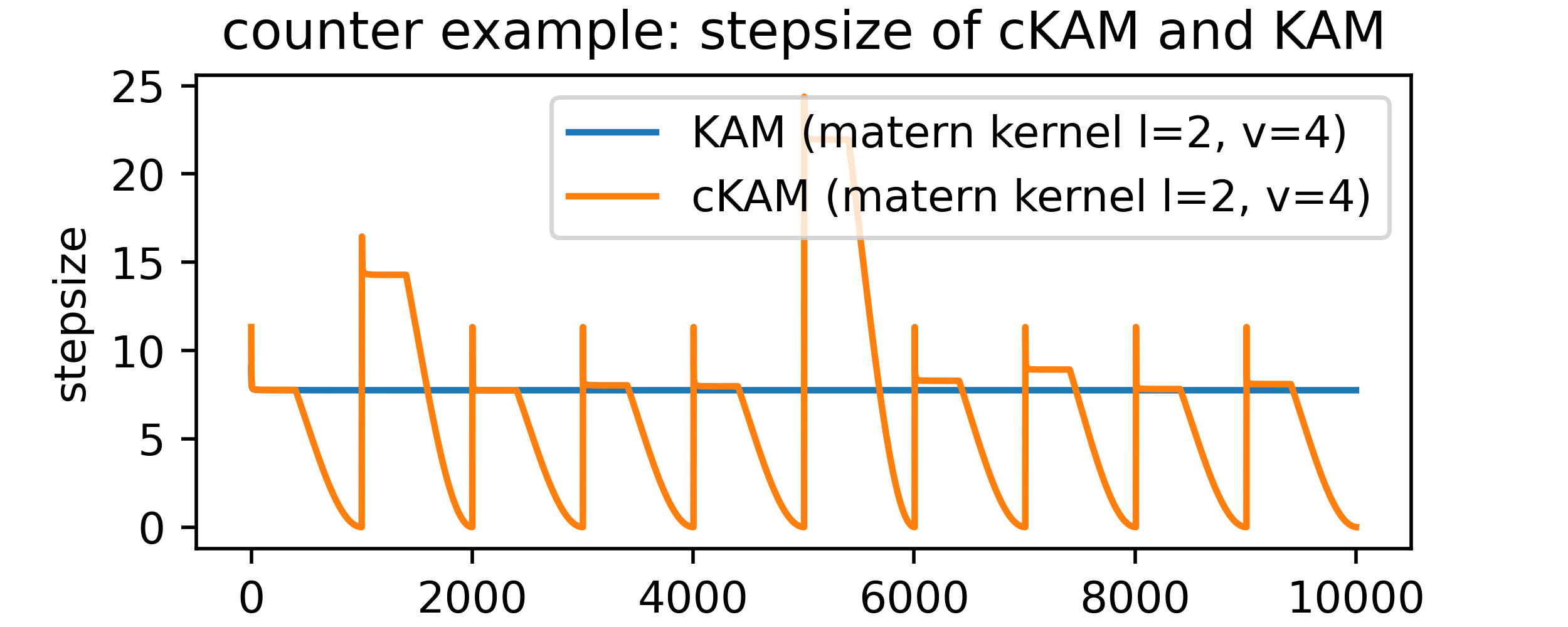
Figure 1: Stepsizes in the first 10 cycles of cKAM and corresponding 10000 iterations of KAM

2.4 Exploration and Sampling in cKAM

Exploration Phase

At Exploration of a cycle, normal KAM proposal is used to propose a next state. With the noise term $\gamma$, initial iterations of this cycle will explore more. We emphasize that this property is made possible by selecting the random subsample $\mathbf{z}$ from the chain history of current cycle. If otherwise, and $\mathbf{z}$ can be selected from the entire chain history, the property of exploration will be lost as the proposed state will depend on the positions in previous cycles close to the current position.

However, we admit that the initial positions in the current cycle would depend on the very last sample in the previous cycle, just like the initial positions in the chain of any other MCMC algorithms would depend on the initial state $\theta_{0}$. One can follow the same analogy made in the cSG-MCMC paper, and think of Exploration as a warm restart to explore a different part of posterior following local covariance structure. By using adaptive stepsizes in this phase, cKAM can experience enough perturbation to escape current mode, and can benefit from a better mixing rate by optimizing for a target acceptance ratio $\alpha^{*}$.

Sampling Phase

The stepsizes in this phase follows the pattern described in 2.3, with a theoretical $\nu_{0}$ computed from the final stepsize in Exploration as if Exploration also used a cyclical stepsize schedule. The stepsize in Sampling decreases rapidly, allow cKAM to better explore the landscape of local regions.

In order to greatly reduce computational cost of making a proposal, we unconventionally change the proposal from KAM proposal to a RW proposal. Although the computation cost of KAM proposal might be still much smaller than evaluation of likelihood functions when using vanilla MH, this reduction will become significant if mini-batched MH algorithms are used, such as TunaMH (Zhang et al., 2020a), FlyMC (Maclaurin & Adams, 2014) and others.

2.5 Ergodicity of cKAM

Here we sketch out a rough proof based on previous works, to show that cKAM samples from the exact posterior distribution.

First, we recognize that cKAM belongs to the framework proposed by Tierney (Tierney, 1994) of MCMC mixture using cycles, where proposals $q_{1},...,q_{k}$, when used individually can lead to the correct target posterior, are used in return in a cycle. Indeed, with a cycle, except for one position collected in the transition from Exploration to Sampling, all others are from draw from either KAM or RW proposals that has been applied with either MH or standard Metropolis. Furthermore, it is obvious to see the irreducibility and aperiodic requirements for the mixture (Tierney, 1994) are satisfied, since KAM proposal is asymmetric. cKAM doesn’t need to show weak convergence in Theorem 2 of (Zhang et al., 2020c) which is intended to show asymptotic bound on the bias and MSE caused by the absence of Metropolis-Hastings in SGLD (Welling & Teh, 2011).

Second, we need to justify for the sudden change in the type of proposal (KAM proposal $\rightarrow$ RW proposal). This change in the type of proposal is seen in algorithms that uses Delayed Rejection (Tierney et al., 1998; Green & Mira, 2001; Haario et al., 2006) where conventionally cheaper-to-compute proposals are tried first and upon rejection, more sophisticated proposals are used. Here we can think of the transition as the KAM proposal taking a first try and always fail, with RW proposal making the second move. Note that if we want to explicitly encode this in our algorithm as in Equation 3 of (Haario et al., 2006) and ensure reversibility, we need to have a position $\theta^{\prime}$ proposed from KAM proposal $q_{\mathbf{z}}(\theta^{\prime}|\theta_{exp})$, forcefully reject it, and propose a second position $\theta^{\prime\prime}$ through random walk $q_{RW}(\theta^{\prime\prime}|\theta^{\prime})$, and accepts it with acceptance probability

$$\min\left\{1,\frac{\uppi(\theta^{\prime\prime})q_{\mathbf{z}}(\theta_{exp}|\theta^{\prime})q_{RW}(\theta_{exp}|\theta^{\prime})[1-\alpha(\theta^{\prime}|\theta^{\prime\prime})]}{\uppi(\theta_{exp})q_{\mathbf{z}}(\theta^{\prime}|\theta_{exp})q_{RW}(\theta^{\prime\prime}|\theta^{\prime})[1-\alpha(\theta^{\prime}|\theta_{exp})]}\right\}$$

We decide to ignore this, since the sample proposed would be exactly the same just with a different acceptance ratio; this is not the case that the sampler suddenly proposes a very distant next position. Any bias introduced from this step will be smoothed out by the rest of the positions in the cycle. We conclude that the cKAM sampler is ergodic.

Furthermore, we are only collecting samples in Sampling, which only used the RW proposal for all the samples. Because of this, one can think of Exploration as finding a good initial state for a RW sampler in each cycle. Rather than continuing adapting a covariance matrix, we take the term $(\gamma^{2}I+\nu^{2}M_{\mathbf{z},\theta_{t}}HM_{\mathbf{z},\theta_{t}}^{T}$ as $\nu^{2}\Sigma)$ to be a fuzzy estimate of local covariance matrix $\Sigma$ for RW proposals.

3 Experiments

We fix our comparison to the following samplers:

• (RW) Random-Walk with isotropic proposal $q(\cdot|\theta_{t})=\mathcal{N}({\cdot|\theta_{t},\nu^{2}I})$ where $\nu$ is the stepsize

• (AM) Adaptive Metropolis with a learned covariance matrix and fixed stepsize (Algorithm 2 in (Andrieu & Thoms, 2008))

• (RBAM) Rao-Blackwellised AM algorithm using the “average position” between $\theta_{t}$ and $\theta^{\prime}|\theta_{t}$ (Algorithm 3 in (Andrieu & Thoms, 2008))

• (GAM) Adaptive Metropolis with a learned covariance matrix and a global stepsize adapting to the optimal acceptance $\alpha^{*}=0.234$ (Algorithm 4 in (Andrieu & Thoms, 2008))

• (KAM) Kernel Adaptive Metropolis-Hastings

• (cKAM) Our cyclical Kernel Adaptive Metropolis

We also implement decaying noise schedule $\gamma_{t}=a(b+t)^{\text{-decay\_rate}}$ for KAM, which is set to a constant of $\gamma=0.2$ in the original KAM paper.

3.1 Difficult 2D Bimodal distribution

To demonstrate the importance of exploration, we here provide a synthetic distribution. We want to emphasize that this is a harder synthetic task than 1) double well experiment used in (Ding et al., 2014; Li et al., 2015; Zhang et al., 2020b) and 2) two-dimensional nonlinear distributions as described in (Sejdinovic et al., 2014; Yin & Zhou, 2018; Zhang et al., 2020b), since our proposed task is a two-dimensional distribution of two more distant modes. The density plot of the true distribution is show in figure 2. The analytical form of the distribution and how we set our hyperparameters are described in appendix A.1.

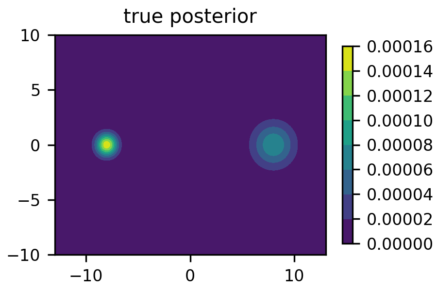
Figure 2: Density plot for the 2d bimodal distribution

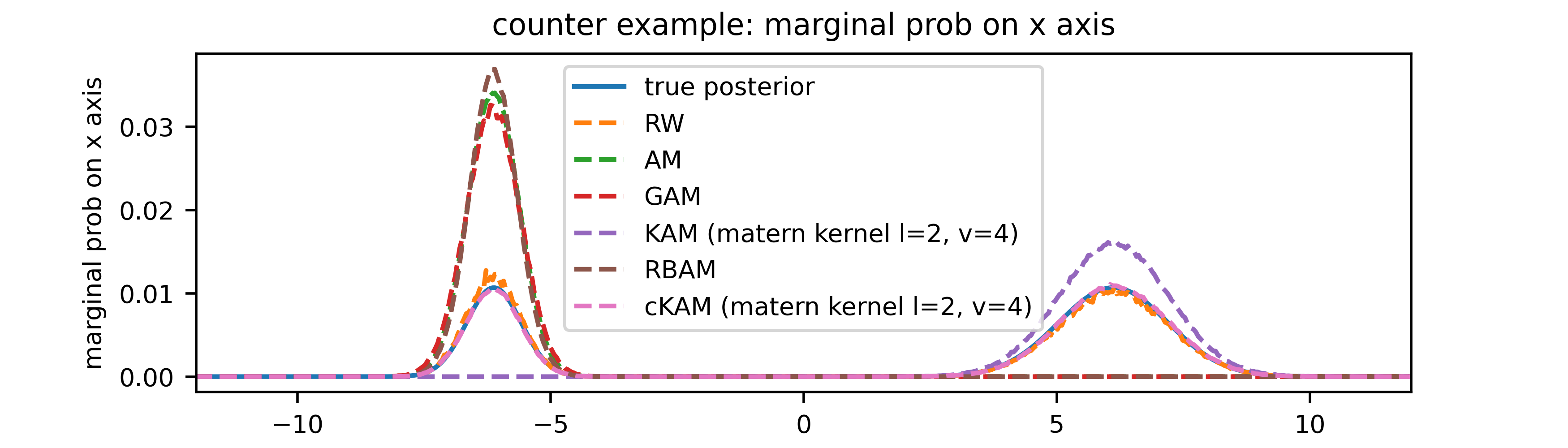
Figure 10: Marginal distribution on the first dimension for all samplers

We plot symmetric Kullback–Leibler (KL) divergence versus wall-clock time after any sample is collected. As can be seen in figure 10 and in appendix A.1, all the adaptive MCMC samplers only converges to one mode. The well-tuned RW (using an extremely unreasonable large $\nu=\sqrt{15}$ as oppose to normal value $2.38/\sqrt{2}$) seems to be asymptotically converging, but is doing so slower than cKAM. While KAM seems to able to escape initialization of $[-8,0]$ due to large initial noise $\gamma_{0}$, it gets trapped in the other mode around $[8,0]$. In contrast, cKAM is able to find and fully explore both modes, regardless of the initial position. cKAM leverages large stepsizes in Exploration to find other modes, and exploits a local mode in Sampling when having smaller stepsizes.

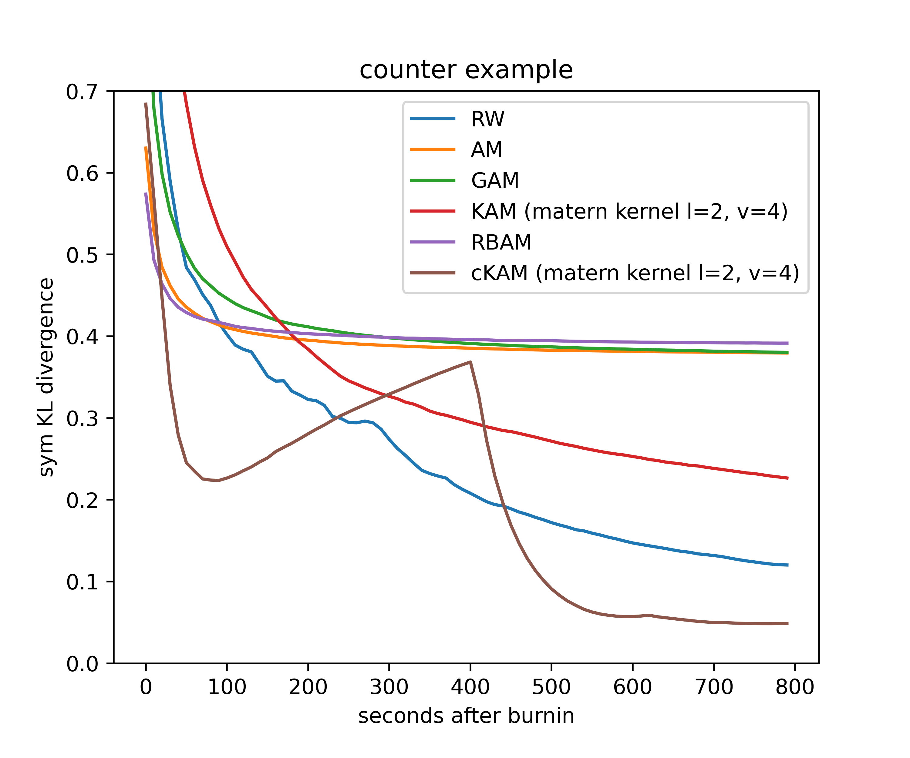
Figure 3: KL divergence against time for all samplers

We continued running cKAM for more time, and it converges to the true posterior as shown below:

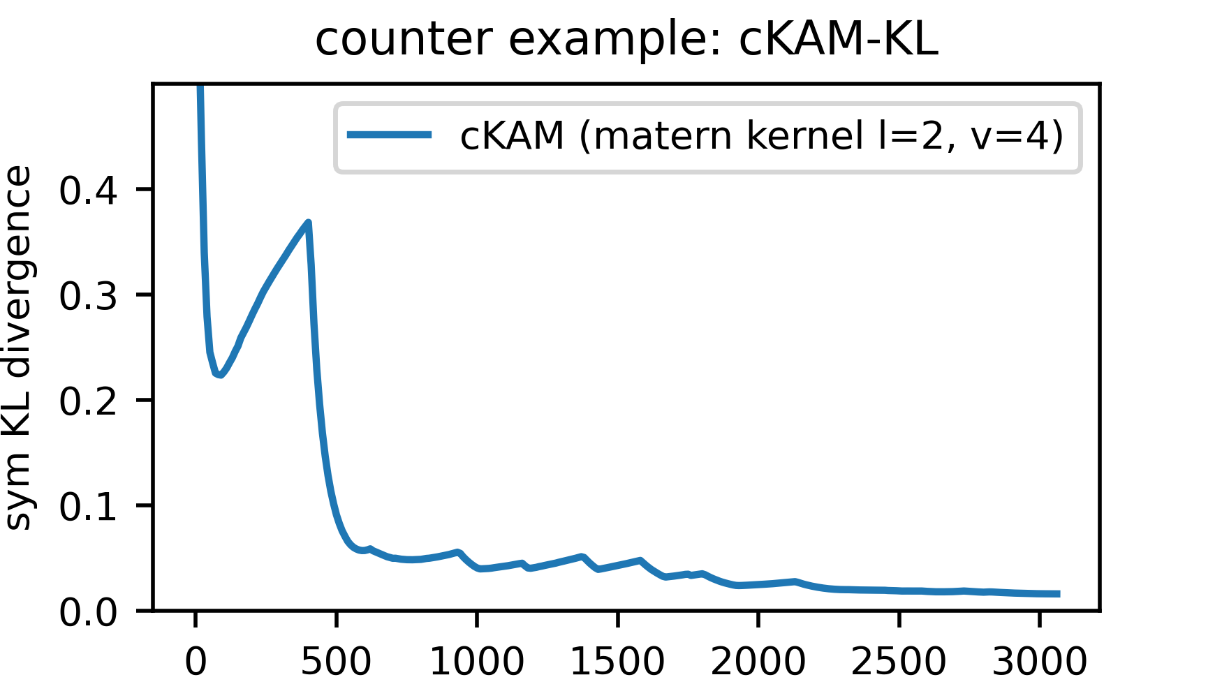
Figure 4: KL divergence against time for cKAM

Figure 4 gives us some intuition behind cKAM’s behavior: around time 100 second, cKAM jumps to another mode which explains the increase in KL divergence. cKAM roughly covers both modes at time 500 second, then it jumps between modes in Exploration and explore the local landscape in Sampling, which explains the small oscillations in the figure. We also show the effect of using different kernels for both KAM and cKAM in appendix A.1.

3.2 2D Gaussian Mixtures with increasing Std

We then proceed with a more realistic setting, where 5 Gaussian distributions with increasing standard deviation. This should be a easier task than the Bimodal one since all individual Gaussians are close to each other. In figure 7 we show its true density plot. The analytical form is given in appendix A.2.

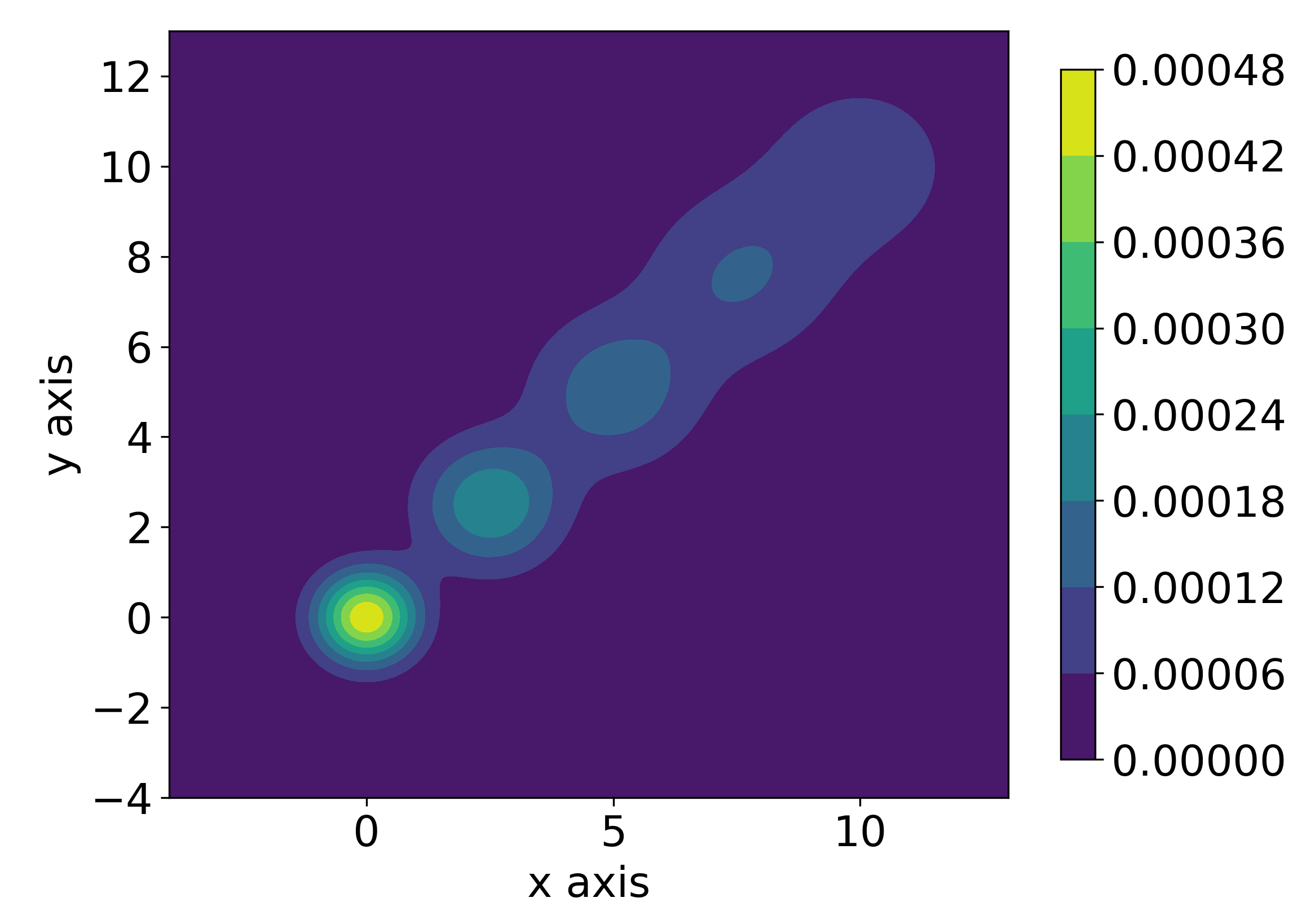
Figure 5: Density plot for the 2d Gaussian Mixtures

We show the KL divergence versus wall-clock time after any sample is collected.

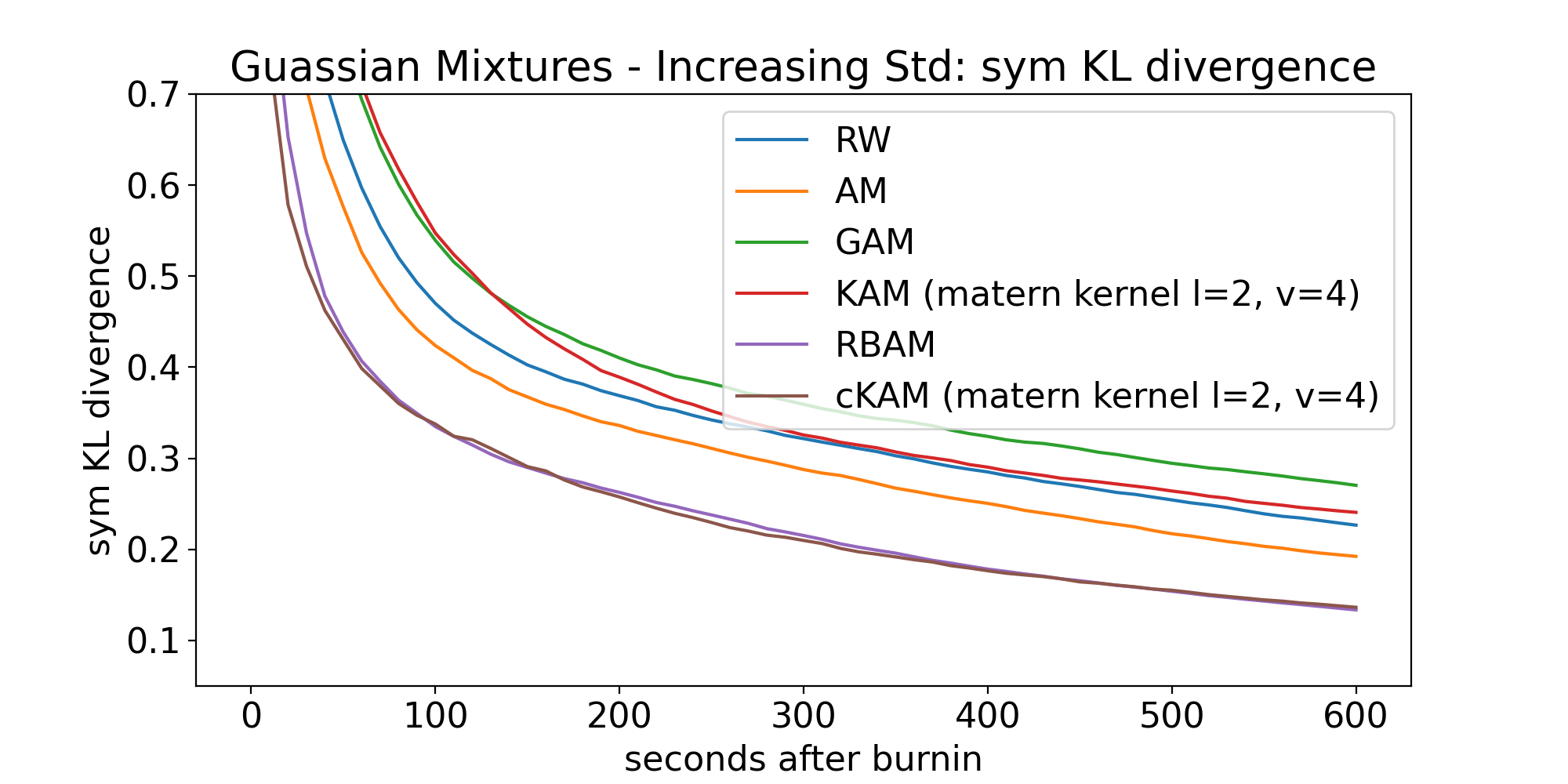
Figure 6: KL divergence against time for all samplers

As can be seen, while all the samplers seem to be asymptotically converging, cKAM is converging faster than KAM, while on par with the best adaptive method RBAM. After running cKAM with more time budget, it converges to the true posterior as show in Figure 7

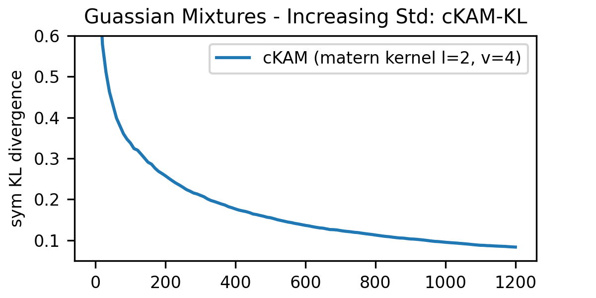
Figure 7: KL divergence against time for cKAM

3.3 High-dimensional Gaussian Mixtures

We construct a 32-dimensional Gaussian Mixtures with $5^{32}$ 32-dimensional Gaussian distributions with different mean and same covariance arranged in a hyper-cube. We plot the marginalized density over dimension 2 and 7.

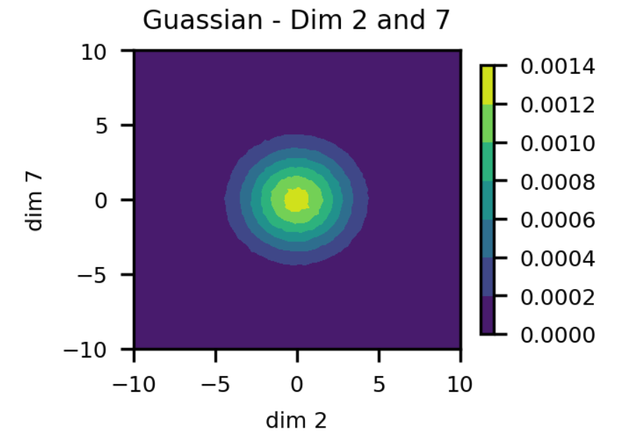
Figure 8: Dimensions 2 and 7 of the high-dimensional Gaussian Mixtures

We show the KL divergence versus wall-clock time after any sample is collected. Due to the curse of dimensionality, it is impossible to generate exact true posterior distribution since it is computationally intractable to build a meshgrid in high-dimensional space (even it the most smallest grid that has 2 slots for each dimension will take $2^{32}*4\text{B}=4\text{GiB}$ memory in total). Since our true posterior distribution is a Gaussian distribution that we know its analytical form in any dimension, we can compute the theoretical marginal posterior probability in one dimension and then compute the symmetric KL divergence with the samples in such dimension. We finally average our results and gain the mean symmetric KL-divergence for such sample.

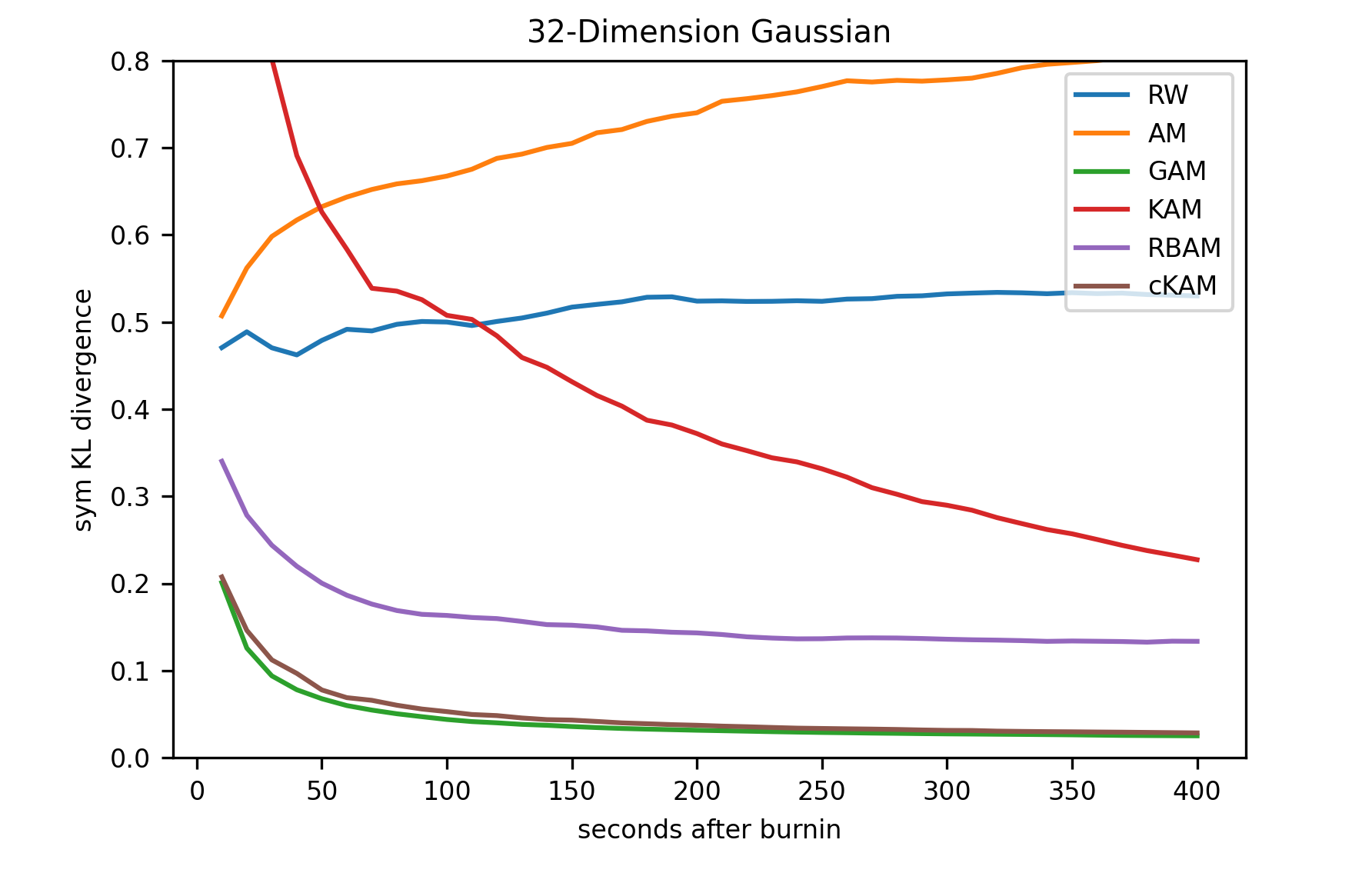
Figure 9: KL divergence against time for all samplers

As can be seen, cKAM outperforms most samplers, with similar performance as GAM. We also observe that during our experiments, the performance of RW proposal was not stable and sometimes it might not converge to the true posterior easily (we needed to tune the initial weights to make RW proposal converge). We guess this might be due to the curse of dimensionality. AM’s KL divergence increases, possibly due to the curse of dimensionality, as the AM sampler explores the posterior poorly, leading to unstable results.

4 Conclusion

We design the cyclical Kernel Adaptive Metropolis (cKAM) algorithm, a variant of the Kernel Adaptive Metropolis-Hastings sampler that allows better exploration of the posterior distribution, while still retaining the local covariance adaptation property. We empirically show that standard adaptive MCMC samplers that continuously conform to either the local or global covariance structure will be incapable of effectively explore multimodal distributions. In experiment, cKAM performs better or on par with well-tuned adaptive samplers, suggesting that our trick of using a fuzzy estimate of local covariance matrix to greatly save computation cost works well in practice. Further extension could include a theoretical convergence analysis on cKAM, and an ablation experiment to demonstrate the importance of using our method compared with proposals that estimate the global covariance, under the cyclical stepsize scheme.

Appendix A EXPERIMENTAL RESULTS

A.1 Difficult 2D Bimodal distribution

We design the two-dimensional distribution to have two modes, each relatively distant from each other. The analytical form of the distribution is:

$$\mathcal{P}(x)=\frac{1}{2}\mathcal{N}\left(x|\mu_{1},\Sigma_{1}\right)+\frac{1}{2}\mathcal{N}\left(x|\mu_{2},\Sigma_{2}\right)$$

Where $\mu_{1}=\begin{bmatrix}-8\\ 0\end{bmatrix},\Sigma_{1}=\begin{bmatrix}0.5&0\\ 0&0.5\end{bmatrix}$ and $\mu_{2}=\begin{bmatrix}8\\ 0\end{bmatrix},\Sigma_{2}=\begin{bmatrix}2&0\\ 0&2\end{bmatrix}$.

We initialize all the samplers from $\mu_{1}$, use a subsample size of 30 for KAM and 50 for cKAM, and run following hyperparameter settings for our samplers:

Table 1: Hyperparameter settings for Bimodal distribution

	(initial) stepsize $\nu$	RM stepsize $\eta$	RM rate $\epsilon$	$T/M$	$\beta$	optimal acceptance $\alpha^{*}$
RW	$\sqrt{15}$	N/A	N/A	N/A	N/A	N/A
AM	$\frac{2.38}{\sqrt{2}}$	0.1	N/A	N/A	N/A	N/A
RBAM	N/A	0.1	N/A	N/A	N/A	N/A
GAM	$\frac{2.38}{\sqrt{2}}$	N/A	0.75	N/A	N/A	0.234
KAM	$\frac{2*2.38}{\sqrt{2}}$	N/A	0.75	N/A	N/A	0.234
cKAM	$\frac{2*2.38}{\sqrt{2}}$	N/A	0.75	1000	0.4	0.234

Where RM refers to Robbins–Monro optimization, where $\eta$ is not the stepsize for proposal, but for adaptation of sampler parameters. $\epsilon$ is vanishing rate of adaptation for $\eta_{t}=(1+t)^{\epsilon}$, used in GAM, KAM and cKAM. RBAM does not need an initial stepsize, but an initial $\Sigma_{0}$, which we set to $I$. We allow KAM and cKAM to have a large initial stepsize of $\frac{2*2.38}{\sqrt{2}}$ to encourage exploration, but because the stepsize is adaptive, as in the case of GAM, we still can have better mixing by optimizing stepsize to have running acceptance ratio $\alpha$ to be close to $\alpha^{*}$. Since we are running our samplers against time, we here do not provide a fixed number of iterations for samplers, but provide $T/M$ which is number of iterations per cycle for cKAM. We use the Matérn Kernel with $l=2$ and $v=4$ for cKAM and KAM when comparing with other methods. Below is the marginal probability of all the samplers, and the true distribution.

We plotted the Effective Sample Size against time for all the samplers:

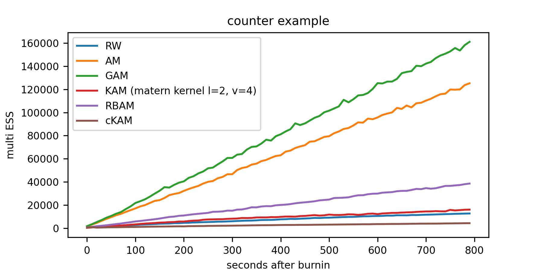
Figure 11: ESS against time

Although cKAM has the lowest ESS per time, this is because all other samplers excepts RW converge to the wrong distribution. We also show all the density plot for the samples collected by different samplers:

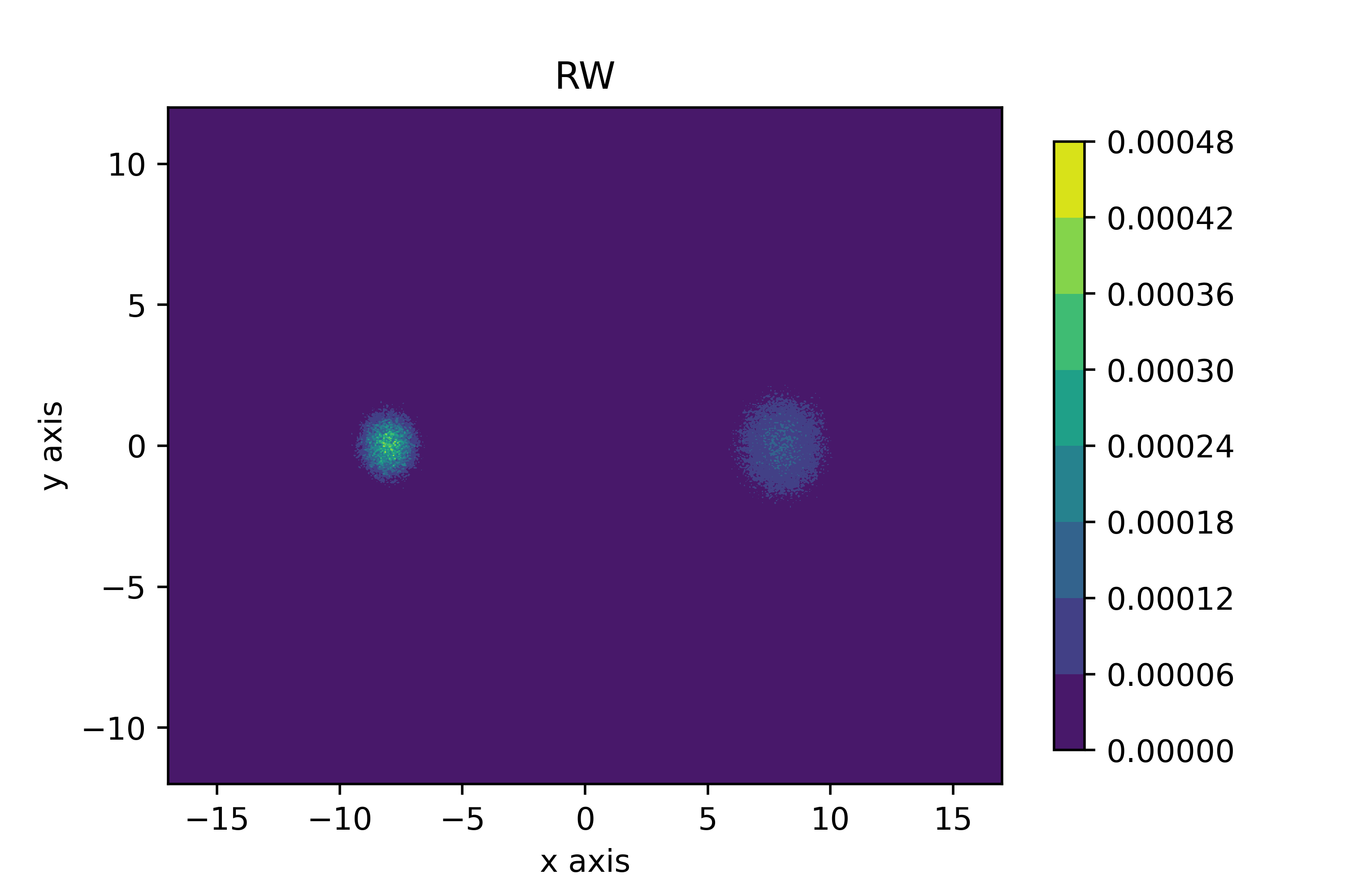
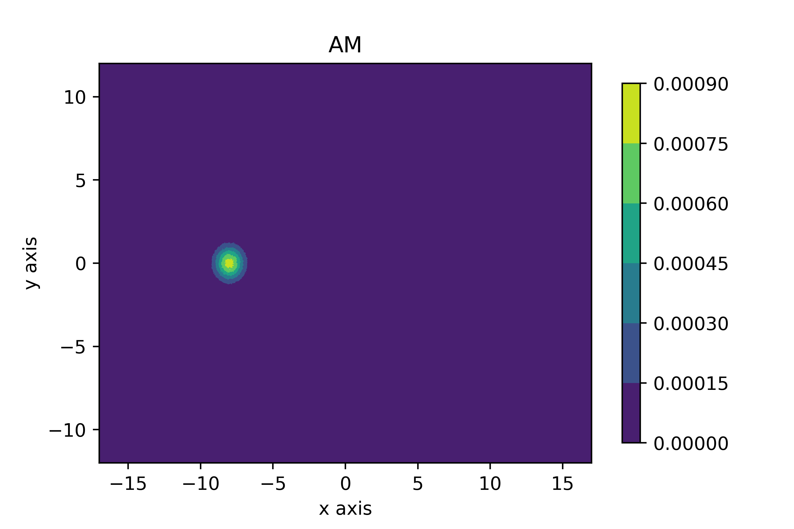
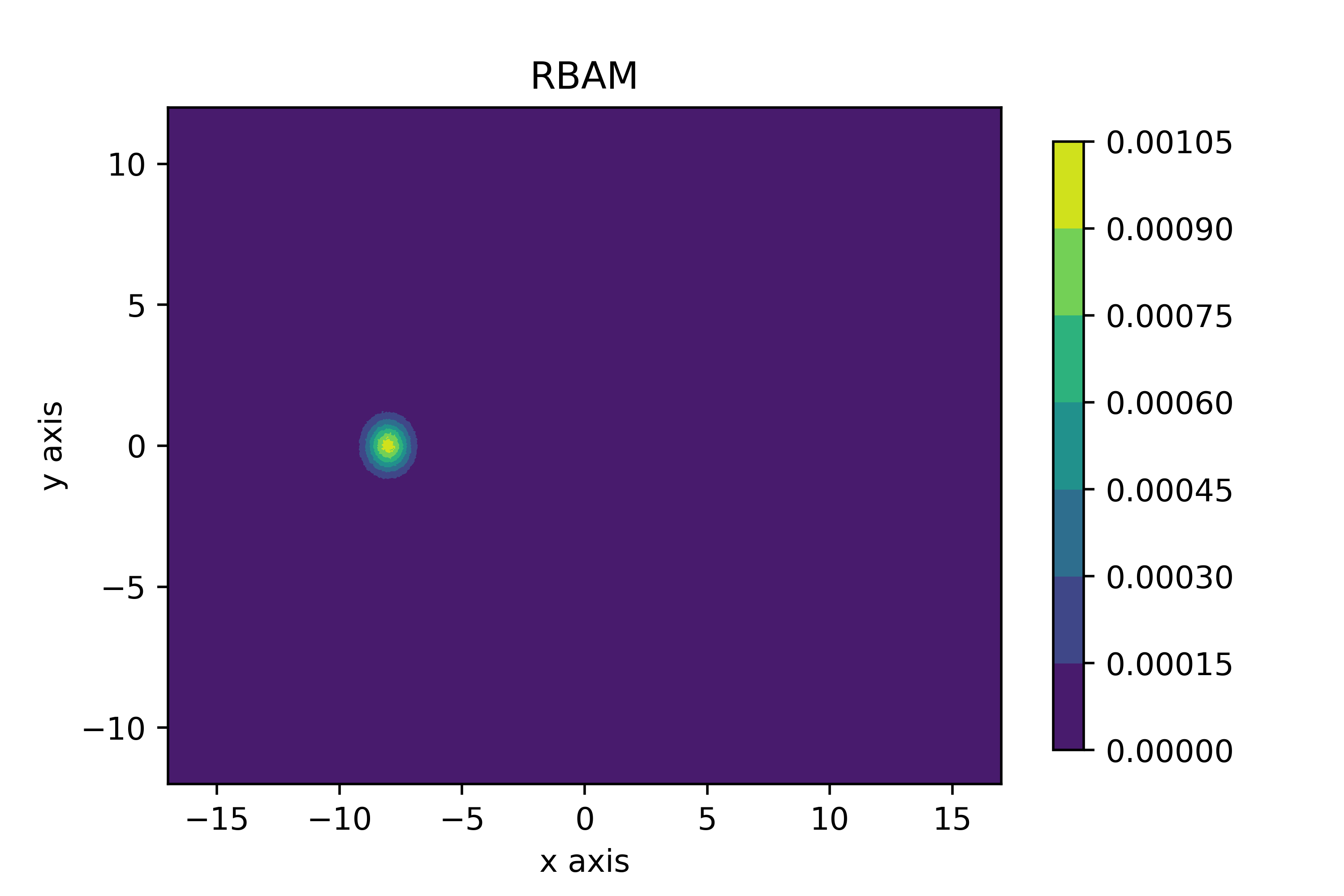
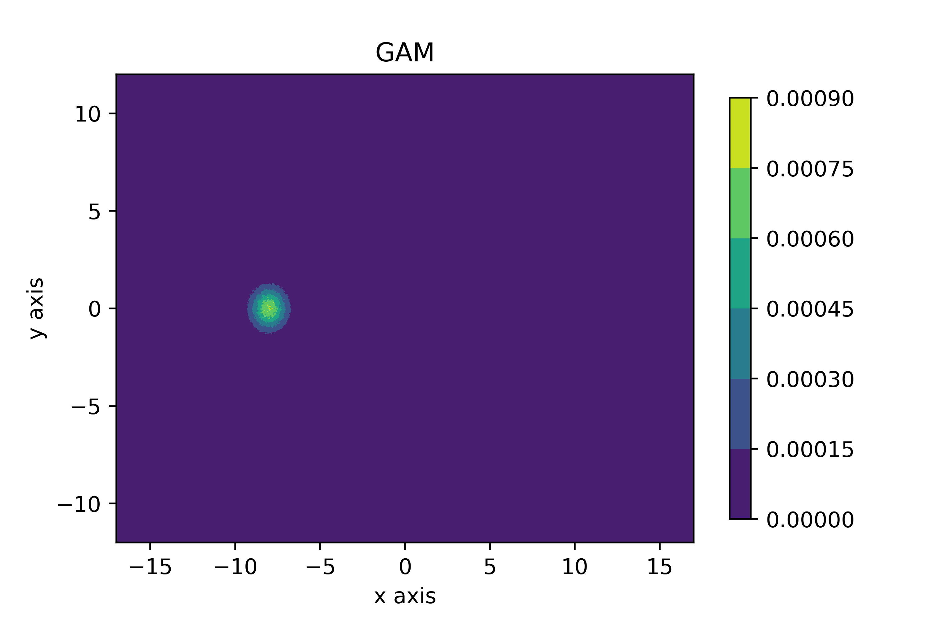
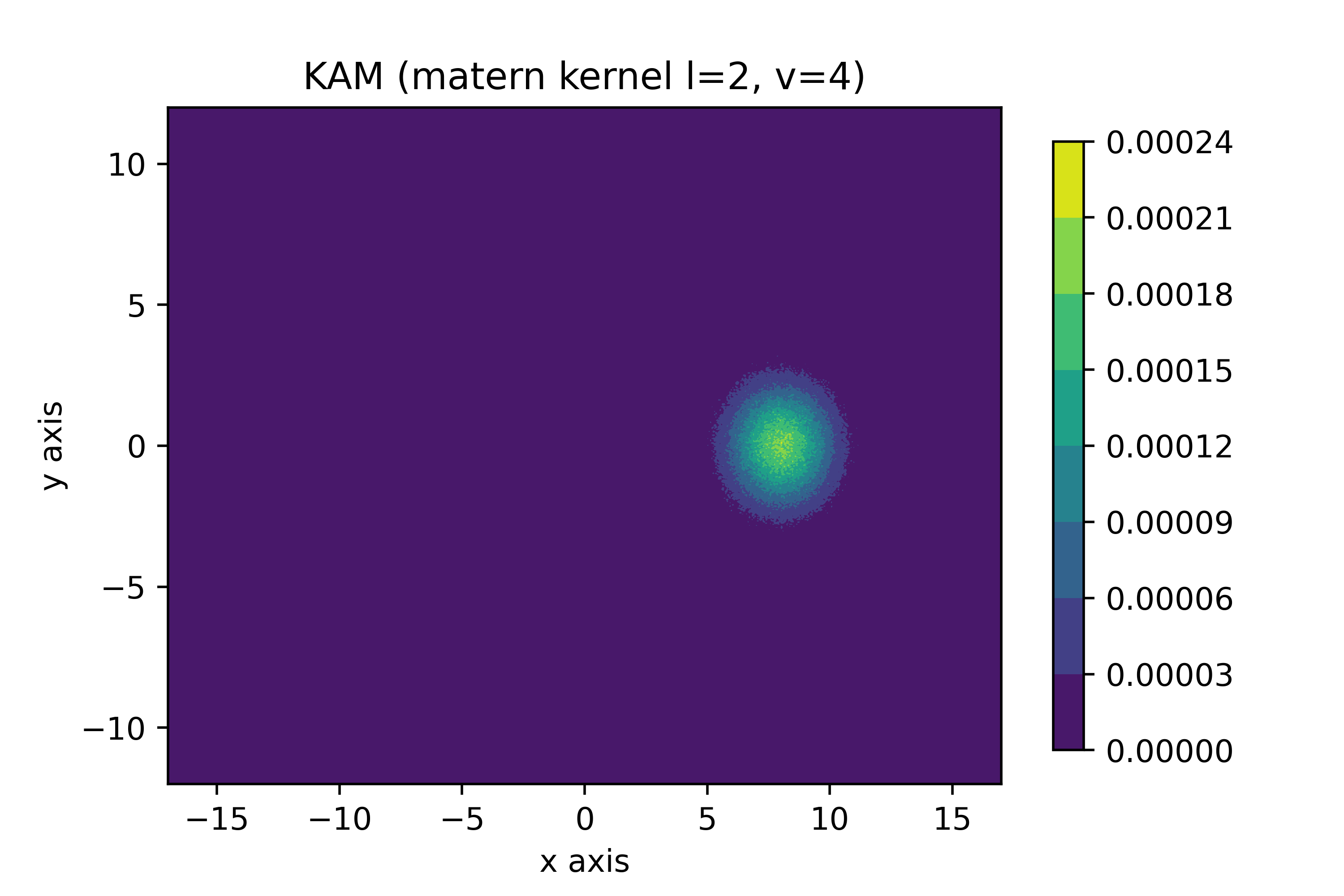
Figure 12: Density plot for all samplers

We discovered empirically that any reasonable choice of kernel does not affect convergence rate for this experiment. We provide results of cKAM running with different kernel abd with all other hyperparameters/parameters kept the same:

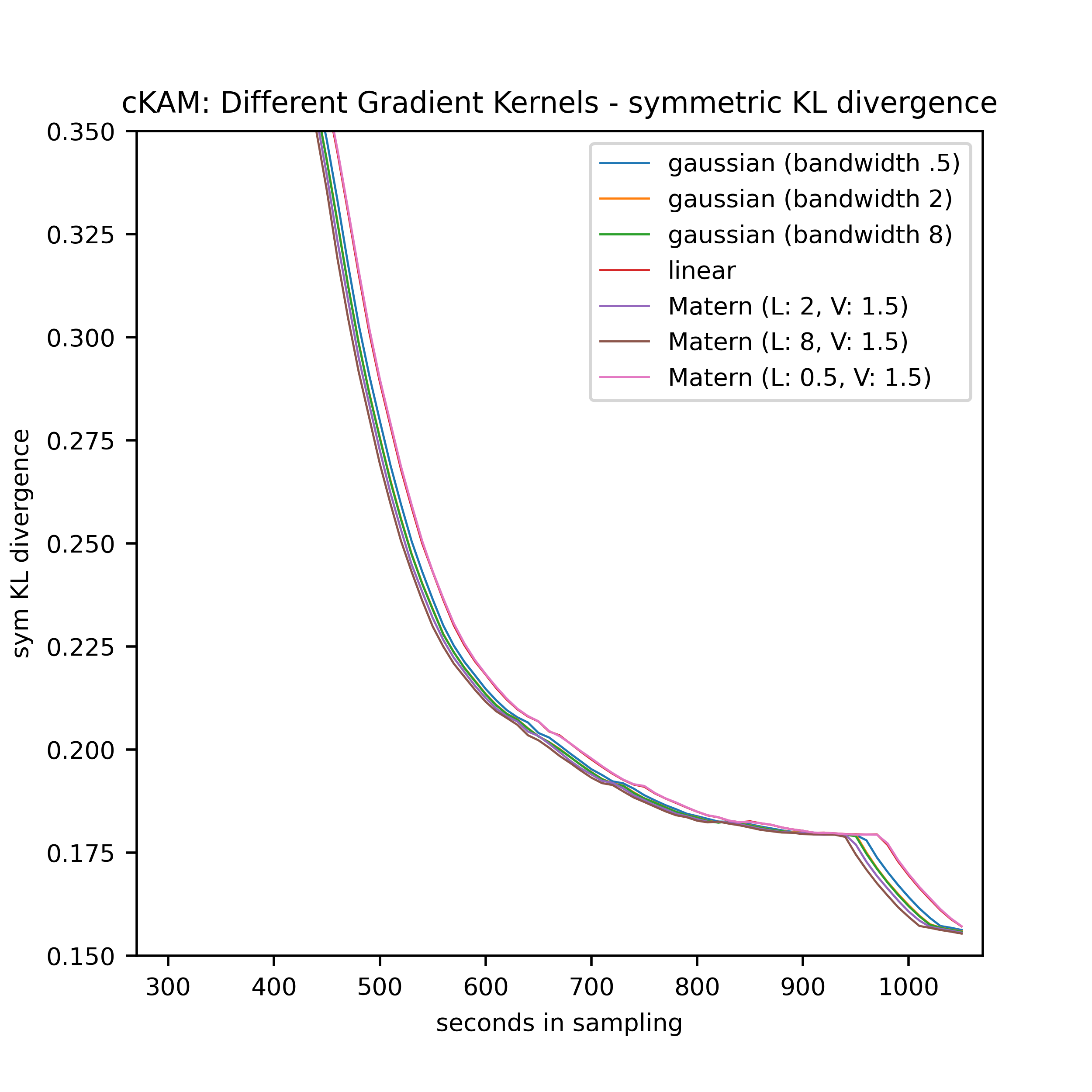
Figure 13: KL divergence against time with different choices of kernel

A.2 2D Gaussian Mixture with increasing standard deviation

We design the two-dimensional distribution composed of 5 Gaussian distributions with increasing standard deviation, leading to the true density plot in figure 7. The analytical form of this distribution is:

$$\mathcal{P}(x)=\frac{1}{5}\sum_{i=1}^{5}\mathcal{N}(x|\mu_{i},\Sigma_{i})$$

Where $\mu_{i}=2.5\begin{bmatrix}i-1\\ i-1\end{bmatrix}$ and $\Sigma_{i}=i^{1/2}\begin{bmatrix}1&0\\ 0&1\end{bmatrix}$. We initialize all the samplers from $[0,0]$, use a subsample size of 30 for KAM and 50 for cKAM, and run following hyperparameter settings for our samplers:

Table 2: Hyperparameter settings for 2D Gaussian Mixture distribution

	(initial) stepsize $\nu$	RM stepsize $\eta$	RM rate $\epsilon$	$T/M$	$\beta$	optimal acceptance $\alpha^{*}$
RW	$\sqrt{15}$	N/A	N/A	N/A	N/A	N/A
AM	$\frac{2.38}{\sqrt{2}}$	0.01	N/A	N/A	N/A	N/A
RBAM	N/A	0.001	N/A	N/A	N/A	N/A
GAM	$\frac{2.38}{\sqrt{2}}$	N/A	0.75	N/A	N/A	0.234
KAM	$\frac{2*2.38}{\sqrt{2}}$	N/A	0.75	N/A	N/A	0.234
cKAM	$\frac{2*2.38}{\sqrt{2}}$	N/A	0.75	1000	0.4	0.234

Since the target distribution is symmetric by design, we also show the marginal probability on the dimension 1 in figure 14.

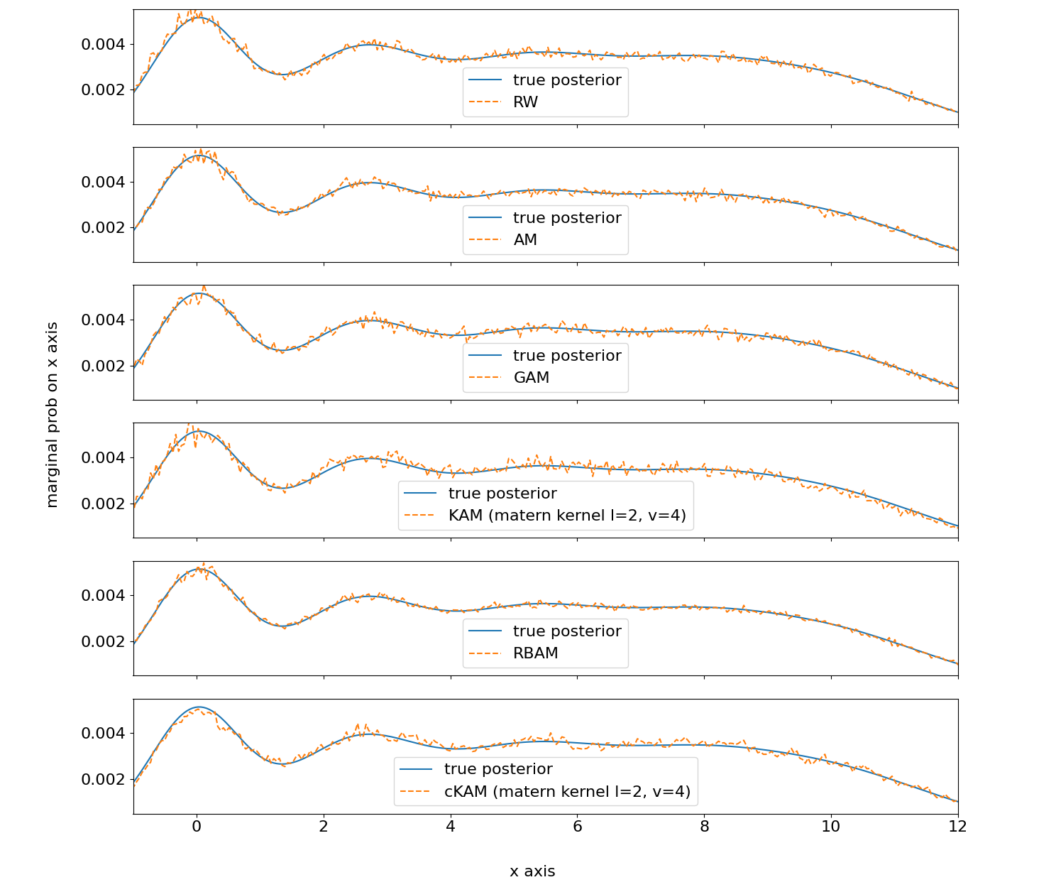
Figure 14: Marginal probability on x-axis for all samplers

A.3 High-Dimensional Gaussian Mixture

We design the 32-dimensional distribution to have $5^{32}$ modes. The analytical form of the distribution is:

$$\mathcal{P}(x)=\sum\mathcal{N}\left(x|\mu,\Sigma\right)$$

Where $\mu=\{-30,15,0,15,30\}^{32},\Sigma$ is a $32\times 32$ identity matrix multiplied by $15$.

We initialize all the samplers from $[0,0]$, use a subsample size of 100 for KAM and 100 for cKAM, and run following hyperparameter settings for our samplers:

Table 3: Hyperparameter settings for 2D Gaussian Mixture distribution

	(initial) stepsize $\nu$	RM stepsize $\eta$	RM rate $\epsilon$	$T/M$	$\beta$	optimal acceptance $\alpha^{*}$
RW	$\frac{2.38}{\sqrt{32}}$	N/A	N/A	N/A	N/A	N/A
AM	$\frac{2.38}{\sqrt{32}}$	0.01	N/A	N/A	N/A	N/A
RBAM	N/A	0.001	N/A	N/A	N/A	N/A
GAM	$\frac{2.38}{\sqrt{32}}$	N/A	0.75	N/A	N/A	0.234
KAM	$\frac{2*2.38}{\sqrt{32}}$	N/A	0.75	N/A	N/A	0.234
cKAM	$\frac{2*2.38}{\sqrt{32}}$	N/A	0.75	8000	0.6	0.234

References

- Andrieu & Thoms (2008) Andrieu, C. and Thoms, J. A. A tutorial on adaptive mcmc. Statistics and Computing, 18:343–373, 2008.
- Atchadé et al. (2011) Atchadé, Y., Fort, G., Moulines, E., and Priouret, P. Adaptive Markov chain Monte Carlo: theory and methods, pp. 32–51. Cambridge University Press, 2011. doi: 10.1017/CBO9780511984679.003.
- Brooks et al. (2011) Brooks, S., Gelman, A., Jones, G., and Meng, X. Handbook of Markov Chain Monte Carlo. Chapman & Hall/CRC Handbooks of Modern Statistical Methods. CRC Press, 2011. ISBN 9781420079425. URL https://books.google.com/books?id=qfRsAIKZ4rIC.
- Chen et al. (2016) Chen, Y., Keyes, D., Law, K. J. H., and Ltaief, H. Accelerated dimension-independent adaptive metropolis. SIAM Journal on Scientific Computing, 38(5):S539–S565, 2016. doi: 10.1137/15M1026432. URL https://doi.org/10.1137/15M1026432.
- Ding et al. (2014) Ding, N., Fang, Y., Babbush, R., Chen, C., Skeel, R. D., and Neven, H. Bayesian sampling using stochastic gradient thermostats. In Ghahramani, Z., Welling, M., Cortes, C., Lawrence, N., and Weinberger, K. Q. (eds.), Advances in Neural Information Processing Systems, volume 27. Curran Associates, Inc., 2014. URL https://proceedings.neurips.cc/paper/2014/file/21fe5b8ba755eeaece7a450849876228-Paper.pdf.
- Green & Mira (2001) Green, P. J. and Mira, A. Delayed rejection in reversible jump Metropolis–Hastings. Biometrika, 88(4):1035–1053, 12 2001. ISSN 0006-3444. doi: 10.1093/biomet/88.4.1035. URL https://doi.org/10.1093/biomet/88.4.1035.
- Haario et al. (2001) Haario, H., Saksman, E., and Tamminen, J. An adaptive metropolis algorithm. Bernoulli, 7(2):223–242, 2001. ISSN 13507265. URL http://www.jstor.org/stable/3318737.
- Haario et al. (2006) Haario, H., Laine, M., Mira, A., and Saksman, E. Dram: efficient adaptive mcmc. Statistics and Computing, 16:339–354, 12 2006. doi: 10.1007/s11222-006-9438-0.
- Li et al. (2015) Li, C., Chen, C., Fan, K., and Carin, L. High-order stochastic gradient thermostats for bayesian learning of deep models, 2015.
- Maclaurin & Adams (2014) Maclaurin, D. and Adams, R. P. Firefly monte carlo: Exact mcmc with subsets of data, 2014.
- Neal (2011) Neal, R. M. Mcmc using hamiltonian dynamics. arXiv: Computation, pp. 139–188, 2011.
- Pompe et al. (2020) Pompe, E., Holmes, C., and Latuszynski, K. A framework for adaptive mcmc targeting multimodal distributions. Annals of Statistics, 48:2930–2952, 10 2020. doi: 10.1214/19-AOS1916.
- Roberts & Rosenthal (1998) Roberts, G. O. and Rosenthal, J. S. Optimal scaling of discrete approximations to langevin diffusions. Journal of the Royal Statistical Society Series B, 60(1):255–268, 1998. URL https://EconPapers.repec.org/RePEc:bla:jorssb:v:60:y:1998:i:1:p:255-268.
- Roberts & Rosenthal (2007) Roberts, G. O. and Rosenthal, J. S. Coupling and ergodicity of adaptive markov chain monte carlo algorithms. Journal of Applied Probability, 44:458 – 475, 2007.
- Roberts & Stramer (2002) Roberts, G. O. and Stramer, O. Langevin diffusions and metropolis-hastings algorithms. Methodology And Computing In Applied Probability, 4:337–357, 2002.
- Sejdinovic et al. (2014) Sejdinovic, D., Strathmann, H., Garcia, M. L., Andrieu, C., and Gretton, A. Kernel adaptive metropolis-hastings, 2014.
- Tierney (1994) Tierney, L. Markov chains for exploring posterior distributions. Annals of Statistics, 22:1701–1728, 1994.
- Tierney et al. (1998) Tierney, L., Mira, A., Methods, M., and Become, H. Some adaptive monte carlo methods for bayesian inference. 07 1998.
- Welling & Teh (2011) Welling, M. and Teh, Y. W. Bayesian learning via stochastic gradient langevin dynamics. In ICML, 2011.
- Yin & Zhou (2018) Yin, M. and Zhou, M. Semi-implicit variational inference, 2018.
- Zhang et al. (2020a) Zhang, R., Cooper, A. F., and Sa, C. D. Asymptotically optimal exact minibatch metropolis-hastings. CoRR, abs/2006.11677, 2020a. URL https://arxiv.org/abs/2006.11677.
- Zhang et al. (2020b) Zhang, R., Cooper, A. F., and Sa, C. D. Amagold: Amortized metropolis adjustment for efficient stochastic gradient mcmc, 2020b.
- Zhang et al. (2020c) Zhang, R., Li, C., Zhang, J., Chen, C., and Wilson, A. G. Cyclical stochastic gradient mcmc for bayesian deep learning, 2020c.