GreenBIQA: A Lightweight Blind Image Quality Assessment Method

Abstract

Deep neural networks (DNNs) achieve great success in blind image quality assessment (BIQA) with large pre-trained models in recent years. Their solutions cannot be easily deployed at mobile or edge devices, and a lightweight solution is desired. In this work, we propose a novel BIQA model, called GreenBIQA, that aims at high performance, low computational complexity and a small model size. GreenBIQA adopts an unsupervised feature generation method and a supervised feature selection method to extract quality-aware features. Then, it trains an XGBoost regressor to predict quality scores of test images. We conduct experiments on four popular IQA datasets, which include two synthetic-distortion and two authentic-distortion datasets. Experimental results show that GreenBIQA is competitive in performance against state-of-the-art DNNs with lower complexity and smaller model sizes.

1 Introduction

Image quality assessment (IQA) aims to evaluate image quality at various stages of image processing such as image acquisition, transmission, and compression. Based on the availability of undistorted reference images, objective IQA can be classified into three categories [12]: full-reference (FR), reduced-referenced (RR) and no-reference (NR). The last one is also known as blind IQA (BIQA). FR-IQA metrics have achieved high consistency with human subjective evaluation. Many FR-IQA methods have been well developed in the last two decades such as SSIM [17] and FSIM [23]. RR-IQA metrics only utilize features of reference images for quality evaluation. In some application scenarios (e.g., image receivers), users cannot access reference images so that NR-IQA is the only choice. BIQA methods attract growing attention in recent years.

Generally speaking, conventional BIQA methods consist of two stages: 1) extraction of quality-aware features and 2) adoption of a regression model for quality score prediction. As the amount of user generated images grows rapidly, a handcrafted feature extraction method is limited in its power of modeling a wide range of image content and distortion characteristics. Recently, due to the strong feature representation capability of deep neural networks (DNNs), DNN-based BIQA methods have been proposed and they have achieved significant performance improvement [19]. Yet, collecting large-scale IQA datasets with user annotations is expensive and time-consuming. Moreover, for IQA datasets of a limited size, DNN-based BIQA methods tend to overfit the training data and do not perform well against the test data. To address this problem, DNN-based solutions often rely on a huge pre-trained network which is trained by a large dataset. The large model size demands high computational complexity and memory requirement. Such a solution cannot be easily deployed at mobile or edge devices, where a lightweight solution is essential. Here, we propose a lightweight BIQA method called GreenBIQA. It aims to achieve high performance that is competitive with DNN-based solutions yet demands much less computing power and memory. To this end, for a video source, GreenBIQA can predict perceptual quality scores frame by frame in real time.

To enlarge the training sample number in GreenBIQA, we first crop distortion-sensitive patches from images. Then, an unsupervised representation determination method is used to obtain a large number of joint spatial-spectral features from each patch. Next, we adopt a supervised feature selection method, called the relevant feature test (RFT) [20], to reduce the dimension of quality-aware features. Finally, an XGBoost [3] regressor is used to predict the final quality scores.

There are two main contributions of this work.

• A novel, lightweight and modularized BIQA method is proposed. The components of GreenBIQA include image augmentation, unsupervised feature determination, supervised quality-aware feature selection, and MOS prediction. It can extract quality-aware features efficiently and yield accurate quality predictions.

• We conduct experiments on four widely-used BIQA datasets to demonstrate the advantages of GreenBIQA. It outperforms all conventional BIQA methods in prediction accuracy. Furthermore, its prediction performance is highly competitive with state-of-the-art DNN-based methods, which is achieved with a significantly smaller model size and at a much faster speed.

The rest of this paper is organized as follows. Related work is reviewed in Sec. 2. GreenBIQA is proposed in Sec. 3. Experimental results are shown in Sec. 4. Finally, concluding remarks are given in Sec. 5.

2 Related Work

Quite a few BIQA methods have been proposed in the last two decades. Existing work can be classified into conventional and DNN-based two categories as reviewed below.

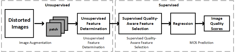
Figure 1: An overview of the proposed GreenBIQA method.

2.1 Conventional BIQA Method

Conventional BIQA methods extract quality-aware features from input images. Then, they train a regression model, e.g., Support Vector Regression (SVR) [1] or XGBoost [3], to predict the quality score based on these features. One representative class of conventional methods relies on the Natural Scene Statistics (NSS). For example, BIQI [14] developed the Distorted Image Statistics (DIS) to capture the NSS changes caused by various distortions. Then, it adopted a distortion-specific quality assessment framework. By following a similar two-stage framework, DIIVINE [15] improved the perceptual quality prediction performance furthermore. Instead of computing distortion-specific features, BRISQUE [13] used scene statistics to quantify loss of naturalness caused by distortions. It operated in the spatial domain with low complexity. Although NSS-based methods are simple, their features are not powerful enough to handle a wide range of distortion types.

Another class of conventional methods leverage the use of codebooks. They share one common framework; namely, local feature extraction, codebook construction, feature encoding, spatial pooling, and quality regression. For instance, CORNIA [21] extracted raw-image-patches from unlabeled images and used clustering to build a dictionary. Then, an image can be represented by soft-assignment coding with spatial pooling of the dictionary. Finally, SVR was adopted to map the encoded quality-aware features to quality scores. By following the same structure, HOSA [18] was developed to improve the performance and reduce the computational cost. Besides the mean of each cluster, some high order statistical information (e.g., dimension-wise variance and skewness) of clusters can also be aggregated to form a small codebook. Codebook-based methods demand high-dimensional handcrafted feature vectors. Again, they cannot handle a wide range of distortion types effectively.

2.2 Deep-learning Based BIQA Method

Deep-learning-based methods have been investigated to solve the BIQA problem. A BIQA method based on the convolutional neural network (CNN), consisting of one convolutional layer with max and min pooling and two fully connected layers was proposed in [7]. To alleviate accuracy discrepancy between FR-IQA and NR-IQA, BIECON [8] used FR-IQA to compute proxy quality scores for image patches and, then, used them to train the neural network. WaDIQaM [2] adopted a deep CNN model that contains ten convolutional layers and two fully connected layers.

Yet, early networks can only handle synthetic distortions (i.e., with given distortion types generated by humans). To achieve better performance, recent work adopts a DNN pre-trained by large datasets. For example, a DNN was pre-tained by the ImageNet [4] and synthetic-distortion datasets in DBCNN [24]. Furthermore, to reflect diverging subjective perception evaluation on an image, PQR [22] adopted a score distribution to represent image quality. A hyper network, which adjusts the quality prediction parameters adaptively, was proposed in HyperIQA [16]. Both local distortion features and global semantic features were aggregated in this work to gather fine-grained details and holistic information, respectively. Afterwards, image quality was predicted based on the multi-scale representation. Despite the good performance of pre-trained DNNs, their huge model sizes are difficult to deploy in many real-world applications.

3 GreenBIQA Method

As shown in Fig. 1, GreenBIQA adopts a modularized solution that consists of the following four modules: (1) image augmentation, (2) unsupervised feature determination, (3) supervised quality-aware feature selection, and (4) MOS prediction. They are elaborated below.

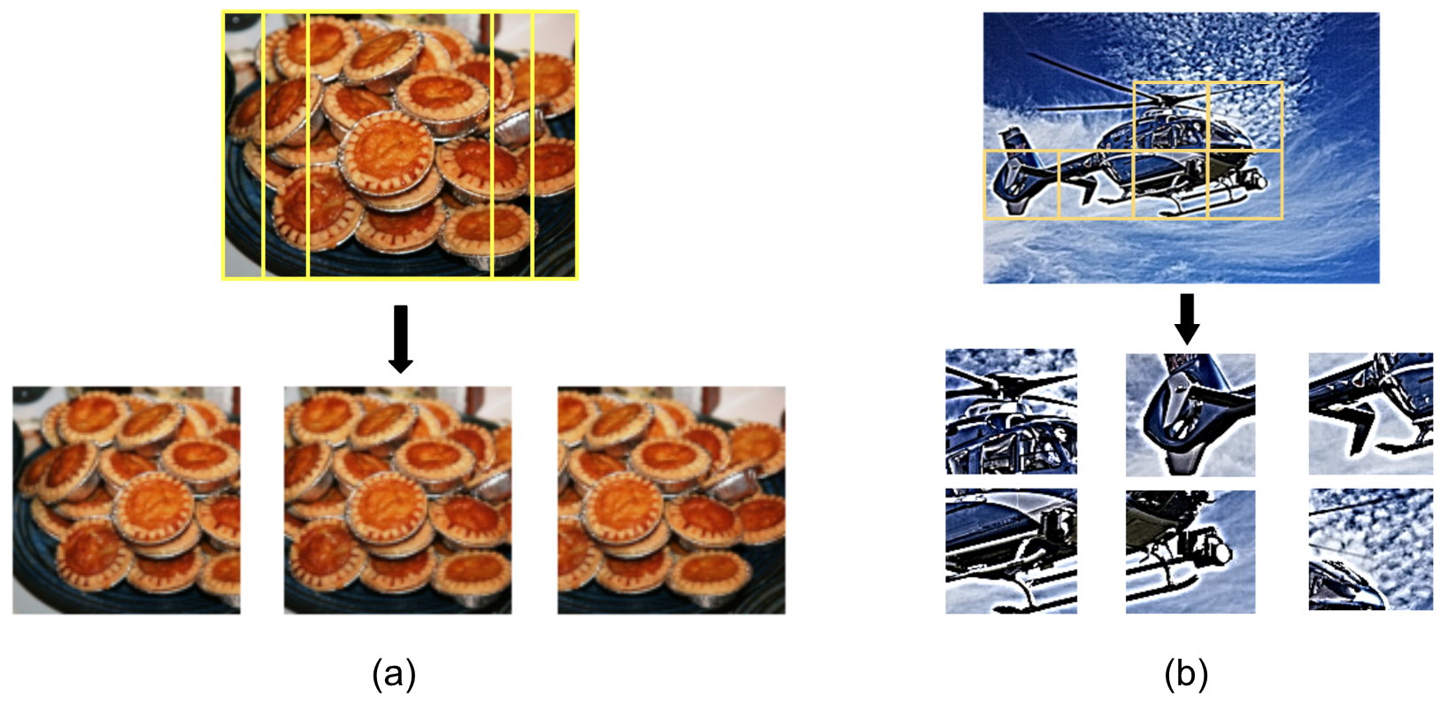
Figure 2: An example of cropped subimages for (a) authentic-distortion and (b) synthetic-distortion datasets.

3.1 Image Augmentation

Image augmentation is implemented to enlarge the number of training samples. This is achieved by image flipping and cropping. All obtained subimages are assigned the same MOS as their source image. To ensure the overall perceptual quality of a subimage, we adopt two different image augmentation strategies for BIQA datasets for authentic-distortions and synthetic-distortions, respectively.

For authentic-distortion datasets such as KonIQ-10K [6], distortions are introduced during capturing. Collected images have a diverse type and a wide range of distortions. Besides, distortions are not uniformly applied to images. To preserve the perceptual quality of subimages and avoid loss of semantic and/or content information, we crop larger subimages out of source images as shown in Fig. 2 (a). The cropped subimages can be overlapped. Each subimage is a squared one. Its size is determined by the height of the source image. We select the left-most, center and right-most three subimages.

In contrast, for synthetic-distortion datasets such as KADID-10K [11], all distortions are added by humans. They are often applied to original undistorted images uniformly with few exceptions (e.g., color distortion in localized regions in KADID-10K). Consequently, we can crop out patches of smaller sizes and treat them as subimages to get even more training samples. An example of non-overlapping cropped patches from an image in KADID-10K is shown in Fig. 2 (b). We select patches that have higher frequency components. Thus, patches containing foreground objects are more likely to be selected than those containing simple background. We feed selected patches to the next module.

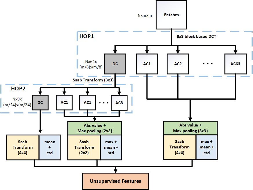
Figure 3: The block diagram of unsupervised feature determination.

3.2 Unsupervised Feature Determination

Given subimages obtained above, we derive a set of features to represent the subimages in an unsupervised manner using a two-hop hierarchy as shown in Fig. 3, where HOP1 and HOP2 are used to capture local and global representations, respectively. Since image and video coding standards all adopt block-based DCT, the processing of GreenBIQA also operates in the DCT domain for faster speed.

In HOP1, we partition an input subimage into non-overlapping blocks of size $8\times 8$ and compute the DCT coefficients of each block. It is done for the Y, U and V channels separately. This step can be skipped if the quality assessment software and the image decoding software can be integrated since the DCT coefficients can be directly obtained from compressed images. DCT coefficients of each block are scanned in the zigzag order, leading to one DC coefficient and 63 AC coefficients, denoted by AC1-AC63. Since the DC coefficients of spatially adjacent blocks are correlated, we apply the Saab transform [9] to decorrelate them in HOP2. Specifically, we partition DC coefficients from HOP1 into non-overlapping blocks of size $3\times 3$. To implement the Saab transform, nine DC coefficients are flattened into a 9-D vector denoted by ${\bf y}=(y_{1},\cdots,y_{9})^{T}$. The mean of the nine DC coefficients, $\bar{y}=(\sum_{i=1}^{9}y_{i})/9$, defines the DC in HOP2. Next, the principle component analysis (PCA) is applied to the mean-removed vector ${\bf y^{\prime}}={\bf y}-\bar{y}(1,\cdots,1)^{T}$ to yield eight AC coefficients, denoted by AC1 to AC8 in HOP2.

There are 63 AC coefficients in each block of HOP1 and 1DC and 8 AC coefficients in each block of HOP2. It is essential to aggregate them spatially to reduce the feature number. To lower the feature dimension, we first take their absolute values and conduct maximum pooling. Next, we adopt the following operations to generate two sets of features.

• Compute the maximum value, the mean value, and the standard deviation of the same coefficient across the spatial domain.

• Conduct the Saab transform on spatially adjacent regions for further dimension reduction and use the Saab coefficients as spectral features.

The above two sets of features are concatenated to form a set of unsupervised features.

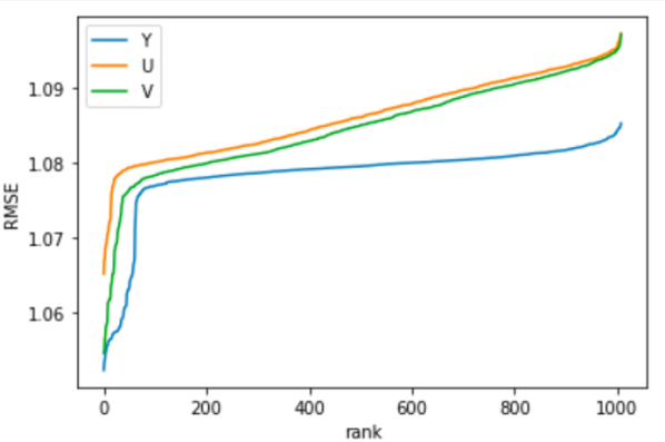
Figure 4: RFT results in Y, U and V three channels.

3.3 Supervised Quality-Aware Feature Selection

To reduce the feature dimension furthermore, we select quality-aware features from the set of unsupervised features obtained in the previous module. This is accomplished by a recently developed method called the relevant feature test (RFT) [20]. For each 1D feature, RFT splits its dynamic range into two subintervals with a certain partitioning point and uses training samples to calculate a cost function. In our current context, we choose the weighted average of root-mean-squared errors (RMSE) of the two subintervals as the cost function. The set of features with the smallest cost functions are selected as quality-aware features. We order features of the smallest to the largest cost functions for Y, U, V three channels in Fig. 4. We see clearly an elbow point in all three curves. We treat feature dimensions before the elbow point as quality-aware features. All selected feature dimensions are concatenated to form the set of quality-aware features.

3.4 MOS prediction

After quality-aware features are selected, we adopt the XGBoost [3] regressor as the quality score prediction model that maps $d$-dimensional quality-aware features to a single quality score. Since we extract $k$ subimages from each image in image augmentation, we have $k$ predicted MOS values for each distorted image. Finally, we adopt a mean filter to ensemble the predictions from all subimages to yield the final MOS prediction for a test distorted image.

4 Experiments

Table 1: Statistics of IQA datasets.

Dataset	Dist.	Ref.	Dist. Types	Scenario
CSIQ [10]	866	30	6	Synthetic
KADID-10K [11]	10,125	81	25	Synthetic
LIVE-C [5]	1,169	N/A	N/A	Authentic
KonIQ-10K [6]	10,073	N/A	N/A	Authentic

4.1 Datasets

We evaluate GreenBIQA on four IQA datasets, including two synthetic datasets and two authentic datasets. Their statistics are given in Table 1. CSIQ [10] and KADID-10K [11] are two synthetic-distortion datasets, where multiple distortions of various levels are applied to a set of reference images. LIVE-C [5] and KonIQ-10K [6] are two authentic-distortion datasets, which contains a diverse range of distorted images captured by various cameras in the real world.

4.2 GreenBIQA Training

We crop 25 patches of size $96\times 96$ and 6 subimages of size $384\times 384$ from images in synthetic- and authentic-distortion datasets, respectively. The number of quality-aware features for each of the Y, U, V channels is set as 2,500, 600, and 600 for authentic and synthetic images, respectively. For the XGBoost regressor, the learning rate is set to 0.05 and the max_depth and number_of_estimators are set to 5 and 1000, respectively. We adopt the early stopping for the XGBoost regressors. All the experiments are run on a server with Intel(R) Xeon(R) E5-2620 CPU.

4.3 Evaluation Metrics

The performance is measured by the Pearson Linear Correlation Coefficient (PLCC) and the Spearman Rank Order Correlation Coefficient (SROCC). PLCC is used to measure the linear correlation between predicted scores and subjective quality scores. It is defined as

$$\textit{PLCC}=1-\frac{\sum_{i}(p_{i}-p_{m})(\hat{p_{i}}-\hat{p_{m}})}{\sqrt{\sum_{i}(p_{i}-p_{m})^{2}}\sqrt{\sum_{i}\hat{p_{i}}-\hat{p_{m}})^{2}}},$$ (1)

where $p_{i}$ and $\hat{p_{i}}$ denote the predicted score and the subjective quality score, $p_{m}$ and $\hat{p_{m}}$ denote the mean of predicted score and the subjective quality score, respectively. SROCC is adopted to measure the monotonicity between predicted and subjective quality scores. It is defined as

$$\textit{SROCC}=1-\frac{6\sum_{i=1}^{L}(m_{i}-n_{i})^{2}}{L(L^{2}-1)},$$ (2)

where $m_{i}$ is the rank of $p_{i}$ in the predicted scores, $n_{i}$ is the rank of $\hat{p_{i}}$ in the subjective quality score and $L$ is the number of images. We adopt the standard evaluation procedure by splitting each dataset into 80% for training and 20% for testing. Furthermore, 10% of training data is used for validation. We run experiments 10 times and report the median PLCC and SROCC values. For synthetic-distortion datasets, splitting is implemented based on reference images to avoid content overlapping.

Table 2: Results on multiple IQA databases.

BIQA Method	CSIQ		LIVE-C		KADID-10K		KonIQ-10K		Model Size
	SROCC	PLCC	SROCC	PLCC	SROCC	PLCC	SROCC	PLCC	(MB)
NIQE [14]	0.627	0.712	0.455	0.483	0.374	0.428	0.531	0.538	-
BRISQUE [13]	0.746	0.829	0.608	0.629	0.528	0.567	0.665	0.681	-
CORNIA [21]	0.678	0.776	0.632	0.661	0.516	0.558	0.780	0.795	7.4
HOSA [18]	0.741	0.823	0.661	0.675	0.618	0.653	0.805	0.813	0.23
BIECON [8]	0.815	0.823	0.595	0.613	-	-	0.618	0.651	35.2
WaDIQaM [2]	0.955	0.973	0.671	0.680	-	-	0.797	0.805	25.2
PQR [22]	0.872	0.901	0.857	0.882	-	-	0.880	0.884	235.9
DBCNN [24]	0.946	0.959	0.851	0.869	0.851	0.856	0.875	0.884	54.6
HyperIQA [16]	0.923	0.942	0.859	0.882	0.852	0.845	0.906	0.917	104.7
GreenBIQA (Ours)	0.925	0.936	0.673	0.689	0.847	0.848	0.812	0.834	1.9

Table 3: SROCC of individual distortion types in CSIQ.

	WN	JPEG	JP2K	FN	GB	CC
BRISQUE [13]	0.723	0.806	0.840	0.378	0.820	0.804
HOSA [18]	0.604	0.733	0.818	0.500	0.841	0.716
WaDIQaM [2]	0.974	0.863	0.947	0.882	0.979	0.923
HyperIQA [16]	0.927	0.934	0.960	0.931	0.915	0.874
GreenBIQA (Ours)	0.937	0.971	0.947	0.928	0.922	0.829

4.4 Performance Benchmarking

We compare the performance of GreenBIQA with four conventional and five deep-learning-based methods, and report their results in Table 2. We divide them into four categories.

• NIQE [14] and BRISQUE [13] use NSS-based handcrafted features.

• CORNIA [21] and HOSA [18] are codebook-learning methods.

• BIECON [8] and WaDIQaM [2] are deep-learning methods without pre-training.

• PQR [22], DBCNN [24], and HyperIQA [16] are deep-learning methods with pre-training.

As shown in Table 2, GreenBIQA outperforms conventional BIQA methods in all four datasets. It also outperforms two deep-learning methods without pre-training in both authentic-distortion datasets. As compared with deep-learning methods with pretraining, GreenBIQA achieves competitive or even better performance in synthetic-distortion datasets (i.e., CSIQ and KADID-10K). Furthermore, we show the SROCC performance of individual distortions in the CSIQ dataset in Table 3. There are six distortion types in CSIQ. The best performer in each category is selected for comparison. GreenBIQA performs especially well for JPEG distortion. This could be attributed to the fact that its features are extracted in the DCT domain. For authentic-distortion datasets, GreenBIQA performs better than traditional deep-learning methods such as BIECON and WaDIQaM, which demonstrates that it can generalize well to diverse distortions. There is a performance gap between GreenBIQA and deep-learning models with pre-training. Yet, these pre-trained models have much larger model sizes as a tradeoff.

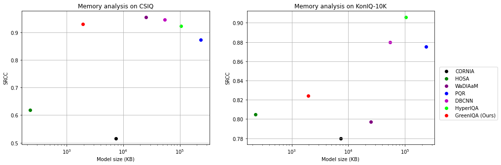
(a) SROCC performance versus the memory size of several benchmarking methods

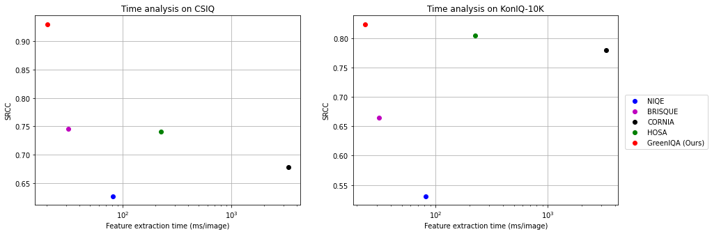
(b) SROCC performance versus the running time of several benchmarking methods

Figure 5: Comparison of (a) model sizes and (b) running time on CSIQ and KonIQ-10K.

4.5 Memory Size Comparison

A small memory size is critical to real-world applications such as mobile phones. To illustrate the tradeoff between performance and memory sizes, we show the SROCC performance versus the memory size (under the assumption that one parameter takes one byte memory) of several benchmarking methods against CSIQ and KonIQ-10K in Fig. 5(a). We see that GreenBIQA can achieve simliar performance on CSIQ and competitive performance on KonIQ-10K. Since high performance deep-learning methods have a huge pre-trained neural network as their backbone, their model sizes are usually more than 100 MB. In contrast, GreenBIQA only needs 600 KB for feature extraction and 1.17 MB for the regression model. Furthermore, GreenBIQA outperforms BIECON and WaDIQaM, which are two deep-learning methods without pre-training, on KonIQ-10K. As compared to codebook-learning methods such as CORNIA and HOSA, whose model sizes are determined by the lengths of the codewords, GreenBIQA achieves much better performance while its size is slightly larger than HOSA and much smaller than CORNIA.

4.6 Running Time Comparison

Another factor to consider for BIQA at the client is running time in MOS prediction. As streaming services and video calls are widely used at mobile devices nowadays, it is desired to assess the quality of individual video frames in real-time with limited computation power. For deep-learning methods with huge pre-trained models, their computations are heavy and have to be run on one or multiple GPUs. To illustrate the tradeoff between performance and running time, we show the SROCC performance versus the MOS inference time per frame of GreenBIQA and four conventional methods on a CPU against CSIQ and KonIQ-10K in Fig. 5(b). Note that we do not include deep-learning-based methods in Fig. 5(b) since they are all implemented on GPUs. GreenBIQA can process around 43 images per second with a single CPU. Thus, it meets the real-time processing requirement. We see from Fig. 5(b) that GreenBIQA has the smallest inference time among all benchmarking methods. It can be executed faster than conventional methods (i.e. NSS-based and codebook-learning methods) with significantly better SROCC performance on both synthetic- and authentic-distortion datasets.

5 Conclusion and Future Work

A lightweight BIQA method, called GreenBIQA, was proposed in this paper. GreenBIQA was evaluated on two synthetic and two authentic datasets. GreenBIQA outperforms all conventional BIQA methods in all datasets. As compared to pre-trained deep-learning methods, GreenBIQA achieves competitive performance with 54x smaller model size. It can extract quality-aware features in real-time (i.e. 43 images per second) using only CPUs. Generally speaking, human annotations of image quality are often limited and difficult to collect. Thus, it is desired to transfer the GreenBIAQ model trained by one model to another one with weak supervision in the future extension.

References

- [1] M. Awad and R. Khanna. Support vector regression. In Efficient learning machines, pages 67–80. Springer, 2015.
- [2] S. Bosse, D. Maniry, K.-R. Müller, T. Wiegand, and W. Samek. Deep neural networks for no-reference and full-reference image quality assessment. IEEE Transactions on image processing, 27(1):206–219, 2017.
- [3] T. Chen and C. Guestrin. Xgboost: A scalable tree boosting system. In Proceedings of the 22nd acm sigkdd international conference on knowledge discovery and data mining, pages 785–794, 2016.
- [4] J. Deng, W. Dong, R. Socher, L.-J. Li, K. Li, and L. Fei-Fei. Imagenet: A large-scale hierarchical image database. In 2009 IEEE conference on computer vision and pattern recognition, pages 248–255. Ieee, 2009.
- [5] D. Ghadiyaram and A. C. Bovik. Massive online crowdsourced study of subjective and objective picture quality. IEEE Transactions on Image Processing, 25(1):372–387, 2015.
- [6] V. Hosu, H. Lin, T. Sziranyi, and D. Saupe. Koniq-10k: An ecologically valid database for deep learning of blind image quality assessment. IEEE Transactions on Image Processing, 29:4041–4056, 2020.
- [7] L. Kang, P. Ye, Y. Li, and D. Doermann. Convolutional neural networks for no-reference image quality assessment. In Proceedings of the IEEE conference on computer vision and pattern recognition, pages 1733–1740, 2014.
- [8] J. Kim and S. Lee. Fully deep blind image quality predictor. IEEE Journal of selected topics in signal processing, 11(1):206–220, 2016.
- [9] C.-C. J. Kuo, M. Zhang, S. Li, J. Duan, and Y. Chen. Interpretable convolutional neural networks via feedforward design. Journal of Visual Communication and Image Representation, 60:346–359, 2019.
- [10] E. C. Larson and D. M. Chandler. Most apparent distortion: full-reference image quality assessment and the role of strategy. Journal of electronic imaging, 19(1):011006, 2010.
- [11] H. Lin, V. Hosu, and D. Saupe. Kadid-10k: A large-scale artificially distorted iqa database. In 2019 Eleventh International Conference on Quality of Multimedia Experience (QoMEX), pages 1–3. IEEE, 2019.
- [12] W. Lin and C.-C. J. Kuo. Perceptual visual quality metrics: A survey. Journal of visual communication and image representation, 22(4):297–312, 2011.
- [13] A. Mittal, A. K. Moorthy, and A. C. Bovik. No-reference image quality assessment in the spatial domain. IEEE Transactions on image processing, 21(12):4695–4708, 2012.
- [14] A. Mittal, R. Soundararajan, and A. C. Bovik. Making a completely blind image quality analyzer. IEEE Signal processing letters, 20(3):209–212, 2012.
- [15] A. K. Moorthy and A. C. Bovik. Blind image quality assessment: From natural scene statistics to perceptual quality. IEEE transactions on Image Processing, 20(12):3350–3364, 2011.
- [16] S. Su, Q. Yan, Y. Zhu, C. Zhang, X. Ge, J. Sun, and Y. Zhang. Blindly assess image quality in the wild guided by a self-adaptive hyper network. In Proceedings of the IEEE/CVF Conference on Computer Vision and Pattern Recognition, pages 3667–3676, 2020.
- [17] Z. Wang, A. C. Bovik, H. R. Sheikh, and E. P. Simoncelli. Image quality assessment: from error visibility to structural similarity. IEEE transactions on image processing, 13(4):600–612, 2004.
- [18] J. Xu, P. Ye, Q. Li, H. Du, Y. Liu, and D. Doermann. Blind image quality assessment based on high order statistics aggregation. IEEE Transactions on Image Processing, 25(9):4444–4457, 2016.
- [19] X. Yang, F. Li, and H. Liu. A survey of dnn methods for blind image quality assessment. IEEE Access, 7:123788–123806, 2019.
- [20] Y. Yang, W. Wang, H. Fu, and C.-C. J. Kuo. On supervised feature selection from high dimensional feature spaces. arXiv preprint arXiv:2203.11924, 2022.
- [21] P. Ye, J. Kumar, L. Kang, and D. Doermann. Unsupervised feature learning framework for no-reference image quality assessment. In 2012 IEEE conference on computer vision and pattern recognition, pages 1098–1105. IEEE, 2012.
- [22] H. Zeng, L. Zhang, and A. C. Bovik. Blind image quality assessment with a probabilistic quality representation. In 2018 25th IEEE International Conference on Image Processing (ICIP), pages 609–613. IEEE, 2018.
- [23] L. Zhang, L. Zhang, X. Mou, and D. Zhang. Fsim: A feature similarity index for image quality assessment. IEEE transactions on Image Processing, 20(8):2378–2386, 2011.
- [24] W. Zhang, K. Ma, J. Yan, D. Deng, and Z. Wang. Blind image quality assessment using a deep bilinear convolutional neural network. IEEE Transactions on Circuits and Systems for Video Technology, 30(1):36–47, 2018.