Possibly heteroclite electron Yukawa coupling and small $\triangle a_{\mu}$ in a hidden Abelian gauge model for neutrino masses

Abstract

We attempt to simultaneously explain the neutrino oscillation data and the observed $(g-2)_{e,\mu}$ in a hidden gauge $U(1)_{X}$ model where all the Standard Model(SM) fields are $U(1)_{X}$ singlets. The minimal version of this model calls for four exotic scalars and two pairs of vector fermions, and all are charged under $U(1)_{X}$. We carefully consider the experimental limits on charge lepton flavor violation without assuming any flavor symmetry and explore the viable model parameter space. The model can accommodate the neutrino oscillation data for both the normal and the inverted mass ordering while explaining the central value of $\triangle a_{e}$ by adopting the fine structure constant determined by using either Cesium or Rubidium atoms. However, mainly constrained by the current experimental bound on ${\cal B}(\tau\rightarrow\mu\gamma)$, this model predicts $\triangle a_{\mu}<5.5(8.0)\times 10^{-10}$ for the normal(inverted) neutrino ordering. Moreover, while the muon Yukawa coupling is close to the SM one, we find the magnitude of the electron Yukawa coupling could be one order of magnitude larger than the SM prediction. This abnormal electron Yukawa could be probed in the future FCC-ee collider and plays an essential role in testing flavor physics.

I Introduction

In the SM of particle physics, the charged fermions acquire their masses after the spontaneous breaking of the $SU(2)_{L}\times U(1)_{Y}$ symmetry via the Higgs mechanism. The fermion masses, $M_{F}$, are fixed by their Higgs Yukawa couplings, $y_{F}$, and $M_{F}=y_{F}v_{0}/\sqrt{2}$, where $v_{0}\sim 246\mathrm{GeV}$ is the SM Higgs vacuum expectation value(VEV). The determination of the Higgs Yukawa couplings of top[1], bottom[2, 3], tau[4, 5], and muon[6, 7] are consistent with the predicted relationship within the errors, typically around a few $\times 10\%$ [8, 9, 10]. The consistency suggests that the origin of masses of the second and the third generation charged fermions can be well accounted by the SM Yukawa interaction. Although theoretically economic and technically natural, the SM does not explain the origin of the observed puzzling mass hierarchy among the charged fermions. Meanwhile, the measurements of Yukawa couplings of other light charged fermions are very challenging due to their smallness or(and) colossal experimental backgrounds. The current upper limit on electron-Yukawa $|y_{e}/y_{e}^{SM}|<260$ [11, 12], obtained from the branching ratio of ${\cal B}(h\rightarrow e^{+}e^{-})$, is relatively poor, and it leaves considerable room for the signal of new physics, see for example[13, 14, 15, 16, 17], which might shed light on the origin of flavor.

The flavor puzzle is not limited to the charged fermion sector only: with undoubtful evidence, at least two out of the three active neutrinos are massive[10]. The observed neutrino masses are about twelve orders of magnitude more diminutive than the electroweak scale. Except for the Dirac CP phase and whether the neutrino mass spectrum ordering is normal or inverted, the neutrino oscillation parameters, three mixing angles and two mass squared differences, have been determined to the precision at the percent level[18]. Despite the tremendous success of the minimal SM, the origin of neutrino masses calls for new degrees of freedom beyond the SM, and we do not know what they are yet. Regardless of the neutrino mass generation mechanism, the well-measured neutrino oscillation parameters are invaluable guides in exploring the unknown territory of flavor physics.

Moreover, the recently measured $(g-2)_{e,\mu}$ appear to deviate from the SM predictions. Combining data from BNL E821 and the result of FNAL gives [20]

$$\triangle a_{\mu}^{F\!N\!A\!L}\simeq(25.1\pm 5.9)\times 10^{-10}\,.$$ (1)

A new measurement at the J-PARC[21] is expected to improve the experimental uncertainty in the near future. Two recent lattice estimations[22, 23] on the hadronic vacuum polarization contribution to $\triangle a_{\mu}$ suggest a result consistent with the experimental data. However, these lattice estimations differ significantly from those based on the dispersion relation[19]. More theoretical studies, see, for example, [24, 25, 26] and references therein, are needed to understand this discrepancy and its consequences.

As for the electron, $\triangle a_{e}$ can be deduced with the input of fine-structure constant $\alpha_{em}$. By adapting $\alpha_{em}$ determined by using Cesium atoms[27], $\triangle a_{e}$ takes the value

$$\triangle a_{e}^{Cs}\simeq(-8.7\pm 3.6)\times 10^{-13}\,.$$ (2)

However, the measurement of $\alpha_{em}$ by using Rubidium atoms[28] yields a result

$$\triangle a_{e}^{Rb}\simeq(+4.8\pm 3.0)\times 10^{-13}\,,$$ (3)

which differs from $\triangle a_{e}^{Cs}$ by $\sim 4\sigma$. It is unclear how to resolve those theoretical and experimental discrepancies associated with $\triangle a_{e,\mu}$ mentioned above. More investigations are needed to settle down the issues. In this work, we try to accommodate $\triangle a_{e}^{Cs}$ and $\triangle a_{e}^{Rb}$ separately and scan our model parameter space to see the prediction of $\triangle a_{\mu}$.

Aiming for a unified explanation for the neutrino mass generation and the anomalous magnetic moments of muon and electron, we consider a dark gauge $U(1)_{X}$ model for the one-loop radiative neutrino mass mechanism. For recent attemps to explain both $\triangle a_{e,\mu}$ and neutrino mass generation, see for example, Refs.[29, 30, 31, 32, 33, 34, 35, 36, 37, 38, 39, 40, 41, 42]. Although we focus on the flavor physics in this work, the potential connection to dark matter is another motivation for us to consider the hidden gauge $U(1)_{X}$. With proper arrangement, the residual parity after spontaneous breaking of $U(1)_{X}$ [43] can be utilized to ensure the stability of the dark matter candidate(s). See [44, 45, 46, 47, 48, 49, 50, 51, 52, 53, 54, 55, 56, 57, 58, 59, 60, 61, 62, 42] for the example implementations of the residual gauge parity on dark matter and neutrino mass generation.

As we will show, the new physics responsible for the neutrino mass generation and $(g-2)_{e,\mu}$ might leave a footprint in the electron-Yukawa. The radiative mechanism for $M_{\nu}$ and $\triangle a_{e,\mu}$ could also lead to sizable charged lepton flavor violation(CLFV) couplings and contradict the stringent experimental constraints, ${\cal B}(l_{i}\rightarrow\gamma l_{j\neq i})$. To avoid introducing further ad hoc assumptions on the flavor pattern, we take a bottom-up approach to investigate what the data say on the model parameter space. We should show that the resulting electron-Yukawa coupling, even its sign, may differ significantly from the SM prediction. Also, the model predicts that $\triangle a_{\mu}\sim 5.5(8.0)\times 10^{-10}$ at most by saturating the current upper limit of ${\cal B}(\tau\rightarrow\mu\gamma)$( and ${\cal B}(\mu\rightarrow e\gamma)$), for normal ordering ( inverted ordering) neutrino mass. If the experimental limits on CLFV processes get improved, this model predicts a even smaller $\triangle a_{\mu}$.

This paper is organized as follows. Our model is detailed in Sec.II, and we also consider the $(g-2)_{e,\mu}$, neutrino mass generation, and the effective Higgs-Yukawa couplings. Sec.III is devoted to the numerical study in that we scan the model parameter space to accommodate the neutrino oscillation data while all the experimental constraints are taken care. Four benchmark configurations and our findings are given therein. In Sec.IV, we discuss some phenomenological considerations with brief comments on the possible dark matter candidates and the prospect of detecting the new gauge boson. Finally, we conclude in Sec.V.

II Model

On top of the SM, our model employs two pairs of vector fermions $N_{1,2}$ and four scalars, $D,C,S_{1},S_{2}$. The new degrees of freedom(DOF) are charged under a hidden gauge $U(1)_{X}$ symmetry. The detailed quantum numbers of the new DOFs are listed in Tab.1. On the other hand, all the SM DOF’s are singlet under the $U(1)_{X}$ such that the $U(1)_{X}$ is “dark”.

	New Fermion				New Scalar
Symmetry$\backslash$ Fields	$N_{1L}$	$N_{1R}$	$N_{2L}$	$N_{2R}$	$D=\begin{pmatrix}D^{0}\\ D^{-}\end{pmatrix}$	$C$	$S_{1}$	$S_{2}$
$SU(2)_{L}$	$1$				$2$	$1$	$1$	$1$
$U(1)_{Y}$	$0$				$-\frac{1}{2}$	$-1$	$0$	$0$
$U(1)_{X}$	$1$				$-1$	$-1$	$-1$	$-2$

Table 1: New field content and quantum number assignment under the SM gauge symmetries $SU(2)_{L}\otimes U(1)_{Y}$, and the gauge $U(1)_{X}$.

The $U(1)_{X}$-invariant renormalizble Yukawa interactions and couplings involving new fermions are

$${\cal L}\supset y^{L}_{ij}\,\overline{L_{i}}DN_{jR}+y^{R}_{ij}\,\overline{e_{Ri}}CN_{jL}-\sum_{i}\frac{1}{2}\left[\xi_{iL}\overline{N^{c}_{iL}}N_{iL}+\xi_{iR}\overline{N^{c}_{iR}}N_{iR}\right]S_{2}-\sum_{ij}\mathfrak{D}_{ij}\overline{N_{iR}}N_{jL}+H.c.$$ (4)

where $\mathfrak{D}_{ij}$ are the new dimensionful Dirac couplings among $N$’s. Here we adopt a convention that $L_{i}$ and $e_{Ri}$ are in the charged lepton flavor(mass) basis. Note that one can choose the diagonal $\xi$’s without losing any generality. The new Yukawa sector enjoys the conventional global lepton number symmetry $U(1)_{L}$ if $\{N,D,C,S_{2}\}$ carry lepton number $\{1,0,0,-2\}$, respectively.

For the scalar sector, the Lagrangian is

$${\cal L} \supset (D_{\mu}H)^{\dagger}(D^{\mu}H)+\mu_{H}^{2}H^{\dagger}H-\lambda_{H}(H^{\dagger}H)^{2}-V_{NP}$$ (5)

$$+ (D_{\mu}D)^{\dagger}(D^{\mu}D)+(D_{\mu}C)^{*}(D^{\mu}C)+(D_{\mu}S_{1})^{*}(D^{\mu}S_{1})+(D_{\mu}S_{2})^{*}(D^{\mu}S_{2})\,,$$

where the new scalar potential is

$$V_{NP} = -\mu_{2}^{2}|S_{2}|^{2}+M_{D}^{2}D^{\dagger}D+M_{C}^{2}|C|^{2}+M_{S_{1}}^{2}|S_{1}|^{2}$$ (6)

$$+ \lambda_{D}(D^{\dagger}D)^{2}+\lambda_{C}|C|^{4}+\lambda_{1}|S_{1}|^{4}+\lambda_{2}|S_{2}|^{4}+\bar{\lambda}_{HD}(D^{\dagger}H)(H^{\dagger}D)$$

$$+ H^{\dagger}H\left(\lambda_{HD}D^{\dagger}D+\lambda_{HC}|C|^{2}+\lambda_{H1}|S_{1}|^{2}+\lambda_{H2}|S_{2}|^{2}\right)$$

$$+ D^{\dagger}D\left(\lambda_{DC}|C|^{2}+\lambda_{D1}|S_{1}|^{2}+\lambda_{D2}|S_{2}|^{2}\right)$$

$$+ |C|^{2}\left(\lambda_{C1}|S_{1}|^{2}+\lambda_{C2}|S_{2}|^{2}\right)+\lambda_{12}|S_{1}|^{2}|S_{2}|^{2}$$

$$+ \sqrt{2}\mu_{DC}H^{\dagger}DC^{*}+\sqrt{2}\mu_{DS}H^{\dagger}\widetilde{D}S_{1}+2\lambda_{4}H^{\dagger}\widetilde{D}S_{2}S_{1}^{*}+\frac{\mu_{12}}{\sqrt{2}}S_{1}^{2}S_{2}^{*}+H.c.$$

The global $U(1)_{L}$ is now explicitly broken by $\lambda_{4}$ and $\mu_{12}$, which are crucial for generating the neutrino Majorana masses. Moreover, since $U(1)_{L}$ is explicitly broken, there is no massless Majoraon associated with the SSB of $U(1)_{X}$ . However, with the presence of $\lambda_{4}$ or $\bar{\lambda}_{HD}$, no simple analytic expression is available for the scalar potential to be bounded from below. In general, one needs to check the positivity condition numerically. For simplicity while keeping the essential physics, we will set $\lambda_{4}=0$ and $\bar{\lambda}_{HD}>0$ in our numerical study.

We assume a 2-stage symmetry breaking. At an energy scale higher than the SM electroweak scale, the $U(1)_{X}$ is broken spontaneously as $S_{2}$ acquires a VEV $\left\langle S_{2}\right\rangle=v_{2}/\sqrt{2}$. The new gauge boson $Z_{X}$ acquires a mass $M_{X}=2g_{X}v_{2}$, where the gauge coupling $g_{X}$ is a free paramter and we assume $v_{2}\gg M_{W}$. The imaginary part of $S_{2}$ is the would-be-Goldstone eaten by the $Z_{X}$ boson. In between the $U(1)_{X}$ breaking scale and the SM electroweak scale, the remaining gauge symmetry is the SM $SU(3)_{c}\times SU(2)_{L}\times U(1)_{Y}$.

The mass term of new fermions becomes ${\cal L}\supset\frac{1}{2}\overline{N^{c}}M_{N}N+H.c.$ where $N=(N_{1L},N^{c}_{1R},N_{2L},N_{2R}^{c})^{T}$, and

$$M_{N}=\left(\begin{array}[]{cccc}\frac{v_{2}\xi_{1L}}{\sqrt{2}}&\mathfrak{D}_{11}&0&\mathfrak{D}_{12}\\ \mathfrak{D}_{11}&\frac{v_{2}\xi_{1R}}{\sqrt{2}}&\mathfrak{D}_{21}&0\\ 0&\mathfrak{D}_{21}&\frac{v_{2}\xi_{2L}}{\sqrt{2}}&\mathfrak{D}_{22}\\ \mathfrak{D}_{12}&0&\mathfrak{D}_{22}&\frac{v_{2}\xi_{2R}}{\sqrt{2}}\end{array}\right)\,.$$ (7)

The symmetric mass matrix $M_{N}$ can be diagonalized by a transformation, $O^{T}M_{N}O$ with eigenvalues $M_{\chi_{i}}(i=1..4)$, and $OO^{\dagger}=O^{\dagger}O=1$. We write the mass eigenstates as $\chi_{L}=(\chi_{1L},\chi_{2L},\chi_{3L},\chi_{4L})$ with $N=O\cdot\chi_{L}$. From $\chi_{L}$, one can construct four Majorana states

$$\chi_{i}=\chi_{iL}+\chi^{c}_{iL}=\chi_{i}^{c}$$ (8)

such that ${\cal L}\supset\frac{i}{2}\overline{\chi}_{i}\not\!\!D\chi_{i}-\frac{1}{2}M_{\chi_{i}}\overline{\chi_{i}}\chi_{i}$. Reversely, the interaction states can be expressed in terms of the physical Majorana states

$$N_{1L}=O_{1i}\hat{L}\chi_{i}\,,\;N_{2L}=O_{3i}\hat{L}\chi_{i}\,,\;N_{1R}=O_{2i}^{*}\hat{R}\chi_{i}\,,\;N_{2R}=O_{4i}^{*}\hat{R}\chi_{i}\,,$$ (9)

where $\hat{L}/\hat{R}=(1\mp\gamma^{5})/2$ is the chiral projection operator. And the Yukawa coupling becomes

$${\cal L}\supset\overline{\chi}_{k}\left(Y_{L}^{ik}\,D^{+}\,\hat{L}+Y_{R}^{ik}\,C^{+}\,\hat{R}\right)l_{i}+\overline{\chi}_{k}\left(Y_{L}^{ik}\,(D^{0})^{*}\,\hat{L}\right)\nu_{i}+H.c.\,,$$ (10)

where

$$Y_{L}^{ik}=\sum_{j=1}^{2}\left(y^{L}_{ij}\right)^{*}O_{(2j)k}\,,\;Y_{R}^{ik}=\sum_{j=1}^{2}\left(y^{R}_{ij}\right)^{*}O^{*}_{(2j-1)k}\,.$$ (11)

In the limit that $\mathfrak{D}_{12},\mathfrak{D}_{21}\ll\mathfrak{D}_{11},\mathfrak{D}_{22},\xi v_{2}$, the mass eigenstates $\chi_{1,2}(\chi_{3,4})$ are mainly composed by $N_{1L,1R}(N_{2L,2R})$. For simplicity, we shall set $\mathfrak{D}_{12,21}=0$ in our numerical study and the physics is more transparent. For a more general case, the full four by four mixing matrix $O$ can be obtained numerically.

Below the SM electroweak symmetry breaking scale, the neutral component of SM Higgs acquires a VEV, $\left\langle H_{0}\right\rangle=v_{0}/\sqrt{2}$. Working in the unitary gauge, $H=[0,(v_{0}+h)/\sqrt{2}]^{T}$, the mixing between $D^{-}$ and $C^{-}$ can be described as a term in Lagrangian

$${\cal L}\supset-(D^{+},C^{+}){\cal M}_{C}\left(\begin{array}[]{c}D^{-}\\ C^{-}\end{array}\right)\,,\;{\cal M}_{C}=\left(\begin{array}[]{cc}\widetilde{M}_{D}^{2}&v_{0}\mu_{DC}\\ v_{0}\mu_{DC}&\widetilde{M}_{C}^{2}\end{array}\right)$$ (12)

where $\widetilde{M}_{D}^{2}=M_{D}^{2}+\frac{1}{2}(\lambda_{HD}+\bar{\lambda}_{HD})v_{0}^{2}+\frac{1}{2}\lambda_{D2}v_{2}^{2}$, and $\widetilde{M}_{C}^{2}=M_{C}^{2}+\frac{1}{2}\lambda_{HC}v_{0}^{2}+\frac{1}{2}\lambda_{C2}v_{2}^{2}$. The charged scalars can be diagonalized by a two-by-two rotation

$$U_{C}=\left(\begin{array}[]{cc}\cos\alpha_{c}&\sin\alpha_{c}\\ -\sin\alpha_{c}&\cos\alpha_{c}\end{array}\right)$$ (13)

with an angle satisfying

$$\sin 2\alpha_{c}={2v_{0}\mu_{DC}\over M_{C2}^{2}-M_{C1}^{2}}\,,$$ (14)

where $M_{C1,C2}$ are the physical mass eigenvalues, and $M_{C2}>M_{C1}$.

The $\lambda_{H2}$ term in Eq.(6) induces a mixing between $h$ and the real part of $S_{2}$. We assume the observed $125\mathrm{GeV}$ Higgs is the lighter physical scalar $h_{SM}$, and the mass of heavier $h_{2}$ is undetermined and not important in this study. The $h\mathchar 45\relax\Re(S_{2})$ mixing results in a universal suppressing factor to the SM $125\mathrm{GeV}$ Higgs couplings. Then the Higgs signal strength becomes $\mu=\cos^{2}\theta_{0}$ with $\theta_{0}$ the mixing angle between $h$ and $\Re(S_{2})$. From $\mu=1.02\begin{subarray}{c}+0.07\\ -0.06\end{subarray}$ obtained by CMS[70] and $\mu=1.06\pm 0.06$ by ATLAS[71], we obtain $\mu=1.042\begin{subarray}{c}+0.047\\ -0.044\end{subarray}$ following the suggestion of [72]. Therefore, one has $\sin^{2}\theta_{0}<0.046$ at 2$\sigma$ C.L. This amounts to $\left|{\lambda_{H2}v_{2}v_{0}\over M^{2}_{h_{2}}-M^{2}_{h_{SM}}}\right|<0.21$ which can be easily satisfied with the model parameters, for example $M_{h_{2}},v_{2}\simeq{\cal O}(\mathrm{TeV})$ and $|\lambda_{H2}|<1$, without much fine-tuning.

Next, the mixings among the neutral components of $D$ and $S_{1}$ can be described by

$${\cal L}\supset-(\Re D^{0},\Re S_{1})\,{\cal M}_{R}\left(\begin{array}[]{c}\Re D^{0}\\ \Re S_{1}\end{array}\right)-(\Im D^{0},\Im S_{1})\,{\cal M}_{I}\left(\begin{array}[]{c}\Im D^{0}\\ \Im S_{1}\end{array}\right)\,,$$ (15)

where

$${\cal M}_{R}=\left(\begin{array}[]{cc}\overline{M}_{D}^{2}&-\mu_{DS}v_{0}\!-\!\lambda_{4}v_{0}v_{2}\\ -\mu_{DS}v_{0}\!-\!\lambda_{4}v_{0}v_{2}&\overline{M}_{S}^{2}+\mu_{12}v_{2}\end{array}\right)\,,\,{\cal M}_{I}=\left(\begin{array}[]{cc}\overline{M}_{D}^{2}&-\mu_{DS}v_{0}\!+\!\lambda_{4}v_{0}v_{2}\\ -\mu_{DS}v_{0}\!+\!\lambda_{4}v_{0}v_{2}&\overline{M}_{S}^{2}-\mu_{12}v_{2}\end{array}\right)\,,$$ (16)

$\overline{M}_{D}^{2}=\widetilde{M}_{D}^{2}-\frac{1}{2}\bar{\lambda}_{HD}v_{0}^{2}$, and $\overline{M}_{S}^{2}=M_{S_{1}}^{2}+\frac{1}{2}\lambda_{H1}v_{0}^{2}+\frac{1}{2}\lambda_{12}v_{2}^{2}$. Note the sign differences in some mass matrix elements for scalar and pseudoscalar, also the mass splitting between $\overline{M}_{D}$ and $\widetilde{M}_{D}$ is about the electroweak scale. Similarly, the real parts and imaginary parts mixing can be diagonalized by the two-by-two rotations $U_{R}$ and $U_{I}$ with angles $\alpha_{R,I}$, and

$$\sin 2\alpha_{R}=-{2(v_{0}\mu_{DS}+\lambda_{4}v_{0}v_{2})\over M_{R2}^{2}-M_{R1}^{2}}\,,\;\;\sin 2\alpha_{I}=-{2(v_{0}\mu_{DS}-\lambda_{4}v_{0}v_{2})\over M_{I2}^{2}-M_{I1}^{2}}\,,$$ (17)

where $M_{R2,R1}$ and $M_{I2,I1}$ are the physical masses of scalars and pseudo scalars made from $D$ and $S_{1}$, respectively. Again, we adopt the convention that $M_{R2}>M_{R1}$ and $M_{I2}>M_{I1}$.

II.1 $\triangle a_{e,\mu}$ and $l_{i}\rightarrow l_{j}\gamma$

In this model, the charged lepton $(g-2)$ receives 1-loop contribution, see Fig.1.

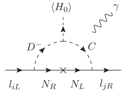
Figure 1: The Feynman diagram, in the interaction basis, for $(g-2)_{l}$ and the CLFV $l\rightarrow l^{\prime}\gamma$ process. The photon attaches to the charged scalar in the loop.

Ignoring the charged lepton mass and summing over all physical states in the loop, the anomalous magnetic dipole moment can be calculated to be[38]

$$\triangle a_{l}=-{m_{l}\sin(2\alpha_{c})\over 16\pi^{2}}\sum_{k=1}^{4}\frac{\Re\left[Y_{L}^{lk}(Y_{R}^{lk})^{*}\right]}{M_{\chi_{k}}}{\cal J}(\beta^{k}_{H},\beta^{k}_{L})\,,$$ (18)

where $\beta^{k}_{H}=(M_{C_{2}}/M_{\chi_{k}})^{2}$, and $\beta^{k}_{L}=(M_{C_{1}}/M_{\chi_{k}})^{2}$. And the loop function is given as

$${\cal J}(x,y)={\cal J}_{0}(x)-{\cal J}_{0}(y)\,,\;{\cal J}_{0}(x)={1-x^{2}+2x\ln x\over 2(1-x)^{3}}\,.$$ (19)

The function ${\cal J}_{0}$ has limits ${\cal J}_{0}(0)=1/2$ and ${\cal J}_{0}(1)=1/6$. On the other hand, the electric dipole moment will be proportional to $\Im\left[Y_{L}^{lk}(Y_{R}^{lk})^{*}\right]$ and stringently limited by the experimental bounds. For simplicity, we should assume there is no extra CP violation phases beyond the SM in the work.

Similarly, the $L(p+q)\rightarrow l(p)+\gamma(q)$ dipole transition amplitude can be read as

$$i{\cal M}^{\mu}_{Ll}=-i\,e\,\overline{u_{l}(p)}\left[\left(d_{L}^{Ll}\hat{L}+d_{R}^{Ll}\hat{R}\right)\left(\frac{i\sigma^{\mu\alpha}q_{\alpha}}{2}\right)\right]u_{L}(p+q)\,,$$ (20)

where

$$d_{L}^{Ll}={\sin(2\alpha_{c})\over 16\pi^{2}}\left\{\sum_{k=1}^{4}\frac{{\cal J}(\beta^{k}_{H},\beta^{k}_{L})}{M_{\chi_{k}}}\left[(Y_{R}^{lk})^{*}Y_{L}^{Lk}\right]\right\}\,,$$

$$d_{R}^{Ll}={\sin(2\alpha_{c})\over 16\pi^{2}}\left\{\sum_{k=1}^{4}\frac{{\cal J}(\beta^{k}_{H},\beta^{k}_{L})}{M_{\chi_{k}}}\left[(Y_{L}^{lk})^{*}Y_{R}^{Lk}\right]\right\}\,.$$ (21)

In terms of the two dipole coefficients, the corresponding CLFV transition rate can be calculated to be[73]

$$\Gamma(L\rightarrow l+\gamma)={\alpha_{em}\,m_{L}^{3}\over 16}\left(|d_{L}^{Ll}|^{2}+|d_{R}^{Ll}|^{2}\right)\,,$$ (22)

if ignoring the mass of the lighter charged lepton. From the current limits: $Br(\mu\rightarrow e\gamma)<4.2\times 10^{-13}$[74], ${\cal B}(\tau\rightarrow e\gamma)<3.3\times 10^{-8}$, ${\cal B}(\tau\rightarrow\mu\gamma)<4.4\times 10^{-8}$[75], $m_{\tau}=1.77686(12)\mathrm{GeV}$, $\tau_{\tau}=(290.3\pm 0.5)\times 10^{-15}s$[10], one has

$$|d_{L}^{\mu e}|^{2}+|d_{R}^{\mu e}|^{2}<2.35\times 10^{-25}(\mathrm{GeV})^{-2}\,,$$

$$|d_{L}^{\tau e}|^{2}+|d_{R}^{\tau e}|^{2}<2.93\times 10^{-17}(\mathrm{GeV})^{-2}\,,$$

$$|d_{L}^{\tau\mu}|^{2}+|d_{R}^{\tau\mu}|^{2}<3.91\times 10^{-17}(\mathrm{GeV})^{-2}\,.$$ (23)

It is clear that to satisfy the stringent experimental bounds, either some couplings are very small or delicate cancellation among the parameters should be arranged. For simplicity and better understanding the physics, we adopt a simple arrangement ${\cal D}_{12,21}=0$ such that the cross mixing between $N_{1}$ and $N_{2}$ vanishes. In this scheme, the charged lepton $g-2$ become

$$\triangle a_{e} = [\cdots]y^{L}_{11}y^{R}_{11}+[\cdots]y^{L}_{12}y^{R}_{12}\,,$$

$$\triangle a_{\mu} = [\cdots]y^{L}_{21}y^{R}_{21}+[\cdots]y^{L}_{22}y^{R}_{22}\,,$$

$$\triangle a_{\tau} = [\cdots]y^{L}_{31}y^{R}_{31}+[\cdots]y^{L}_{32}y^{R}_{32}\,,$$ (24)

where $[\cdots]$ represent the numerical factors depending on $M_{\chi}$, $M_{C,R,I}$, and the mixings. Moreover, once $y^{L}$’s and the relevant physical masses and mixings are fixed, the CLFV dipole transition coefficients have simple dependence on the right-handed Yukawa $y^{R}$:

$$d_{L}^{\mu e}=(\cdots)y^{R}_{11}+(\cdots)y^{R}_{12}\,,\;d_{R}^{\mu e}=(\cdots)y^{R}_{21}+(\cdots)y^{R}_{22}\,,$$

$$d_{L}^{\tau e}=(\cdots)y^{R}_{11}+(\cdots)y^{R}_{12}\,,\;d_{R}^{\tau e}=(\cdots)y^{R}_{31}+(\cdots)y^{R}_{32}\,,$$

$$d_{L}^{\tau\mu}=(\cdots)y^{R}_{21}+(\cdots)y^{R}_{22}\,,\;d_{R}^{\tau\mu}=(\cdots)y^{R}_{31}+(\cdots)y^{R}_{32}\,,$$ (25)

where $(\cdots)$ represent the numerical factors depending on $y^{L}$, $M_{\chi}$, $M_{C,R,I}$, and the mixings. One can set $y^{R}_{31}=y^{R}_{32}=0$ to suppress the CLFV dipole transition, with vanishing $\triangle a_{\tau}$, $d_{R}^{\tau\mu}$, and $d_{R}^{\tau e}$.

II.2 Radiative contributions to the lepton masses

The same Feynman diagram displayed in Fig.1 will generate radiative corrections to the charged lepton mass matrix if the external photon line is removed. A simple calculation gives

$$\delta M_{ij}^{loop}=-\sum_{k}{M_{k}(Y^{ik}_{L})^{*}Y^{jk}_{R}\over 32\pi^{2}}\sin 2\alpha_{c}\left({\beta^{k}_{L}\log\beta^{k}_{L}\over\beta^{k}_{L}-1}-{\beta^{k}_{H}\log\beta^{k}_{H}\over\beta^{k}_{H}-1}\right)$$ (26)

where the first (second) index stands for the left (right)-handed lepton.

To be consistent with the working assumption that the Yukawa couplings, $y^{L,R}$ in Eq.(4), are in the charged leptons’ mass basis, it is required that the tree-level Yukawa coupling between the charged leptons and the SM Higgs doublet, ${\cal L}\supset-y^{H}_{ij}\bar{L}_{i}e_{Rj}H+H.C.$, must satisfy the following relationship

$$\frac{v_{0}}{\sqrt{2}}y^{H}_{ij}+\delta M_{ij}^{loop}=\delta_{ij}m_{i}\,,\;\;\;i=(e,\mu,\tau)\,.$$ (27)

Such that the off-diagonal entries of charged lepton mass matrix vanish, and our treatment is self-consistent at the one-loop level.

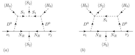
Figure 2: Some leading Feynman diagrams, in the interaction basis, for generating the neutrino masses.

For neutrino masses, they can be radiatively generated by the 1-loop diagrams shown in Fig.2, in the interaction basis. Summing over all mass eigenstates in the loop, we obtain the neutrino mass matrix element

$${\cal M}^{\nu}_{ij}=\frac{1}{16\pi^{2}}\sum_{k=1}^{4}M_{\chi_{k}}\,Y_{L}^{ik}Y_{L}^{jk}\times\sum_{a=1}^{2}\left[\left(U^{R}_{1a}\right)^{2}{s_{ak}\ln s_{ak}\over s_{ak}-1}-\left(U^{I}_{1a}\right)^{2}{p_{ak}\ln p_{ak}\over p_{ak}-1}\right]\,,$$ (28)

where $s_{ak}=(M_{Ra}/M_{\chi_{k}})^{2}$ and $p_{ak}=(M_{Ia}/M_{\chi_{k}})^{2}$ are the mass squared ratios of scalar and pseudoscalar to the Majorana fermion-$k$, respectively.

II.3 Effective Yukawa coupling of charged lepton

Note that the one-loop $h_{SM}\mathchar 45\relax\bar{l}_{i}\mathchar 45\relax l_{j}$ couplings can be generated if replacing the external photon in Fig.1 by the $125\mathrm{GeV}$ SM Higgs, and therefore the tree-level SM prediction $y_{l}=\frac{m_{l}}{v_{0}}$ will be modified. Although the new Yukawa couplings are in the charged lepton mass basis at 1-loop level, the different loop integration involved leads to CLFV Higgs decays $h_{SM}\rightarrow l_{i}l_{j}$ in general.

Below the electroweak scale, the dimensionful cubic couplings for ${\cal L}\supset-\widetilde{\mu}_{ab}\,h_{SM}\,C^{+}_{a}C^{-}_{b}$ can be read from the scalar potential, Eq.(6), as

$$\widetilde{\mu}_{11} = v_{0}(\lambda_{HD}+\bar{\lambda}_{HD})c_{\alpha}^{2}+v_{0}\lambda_{HC}s_{\alpha}^{2}-2s_{\alpha}c_{\alpha}\mu_{DC}$$

$$\widetilde{\mu}_{22} = v_{0}(\lambda_{HD}+\bar{\lambda}_{HD})s_{\alpha}^{2}+v_{0}\lambda_{HC}c_{\alpha}^{2}+2s_{\alpha}c_{\alpha}\mu_{DC}$$

$$\widetilde{\mu}_{12} = \widetilde{\mu}_{21}=v_{0}(\lambda_{HD}+\bar{\lambda}_{HD})s_{\alpha}c_{\alpha}-v_{0}\lambda_{HC}s_{\alpha}c_{\alpha}+(c_{\alpha}^{2}-s_{\alpha}^{2})\mu_{DC}\,,$$ (29)

in the mass basis of the charged scalars. If ignoring the charged lepton masses, the dimensionless $h_{SM}\mathchar 45\relax\bar{l}_{i}\mathchar 45\relax l_{j}$ Yukawa couplings can be calculated to be

$$y_{ij}^{loop}=\frac{1}{16\pi^{2}}\sum_{k=1}^{4}(Y_{L}^{ik})^{*}Y_{R}^{jk}\sum_{a,b=1}^{2}\frac{\widetilde{\mu}_{ab}}{M_{\chi_{k}}}\,U^{C}_{2a}\,U^{C}_{1b}\,{\cal I}_{3}\left(\beta^{a}_{k}\,,\,\beta^{b}_{k}\,,\,\frac{q^{2}}{M_{\chi_{k}}^{2}}\right)$$ (30)

where $q$ is the momentum carried by $h_{SM}$, and

$${\cal I}_{3}(z_{1},z_{2},z_{3})=\int^{1}_{0}dx\int^{1-x}_{0}dy(1-x-y+xz_{1}+yz_{2}-xyz_{3})^{-1}\,.$$ (31)

The analytic expression for ${\cal I}_{3}(a_{1},a_{2},0)$ can be easily obtained and will not be shown here.

Combining with the tree-level Higgs Yukawa, Eq.(27), we obtain the effective Yukawa

$$y^{eff}_{ij}=\frac{y^{H}_{ij}}{\sqrt{2}}+y_{ij}^{loop}=\frac{1}{v_{0}}(\delta_{ij}m_{i}-\delta M^{loop}_{ij})+y_{ij}^{loop}\,.$$ (32)

For $i\neq j$, the CLFV decay width of $h_{SM}\rightarrow l_{i}l_{j}$ is given by

$$\Gamma(h_{SM}\rightarrow l_{i}^{+}l_{j}^{-})=\Gamma(h_{SM}\rightarrow l_{i}^{-}l_{j}^{+})\simeq\frac{M_{h}}{16\pi}\left(|y^{eff}_{ij}|^{2}+|y^{eff}_{ji}|^{2}\right)$$ (33)

at tree-level if ignoring the charged lepton masses. And for the diagonal ones, it is convenient to define the normalized Yukawa

$$\zeta_{l}\equiv\frac{y^{eff}_{l}}{y^{SM}_{l}}=1-\frac{1}{m_{l}}\left(\delta M^{loop}_{ll}-v_{0}\,y_{ll}^{loop}\right)\,.$$ (34)

III Numerical study

First, we comment on the number of exotic vector fermions $N$’s. For the three active neutrinos, one needs six independent parameters to describe the symmetric neutrino mass matrix. Thus, the minimal setup of our model calls for two pairs of exotic fermions, with six $y^{L}$’s paramters. However, it is easy to see from Eq.(28) that the resulting neutrino mass matrix has rank 2. Namely, the neutrino mass matrix possesses only five independent parameters. One of the $y^{L}$’s is redundant and must be fixed first so the rest five can be uniquely determined by data. And the remaining six $y^{R}$’s are used to yield $\triangle a_{e,\mu}$ while satisfying all the experimental CLFV constraints.

With three pairs of exotic fermions, the rank of the neutrino mass matrix is 3. Hence, three out of the nine $y^{L}$ free parameters are redundant. Moreover, with nine $y^{R}$’s parameters, one can always find a viable solution such that all the CLFV limits are satisfied and both central values of $\triangle a_{\mu}$ and $\triangle a_{e}^{Cs[Rb]}$ are accommodated. Such scenario has more free parameters than experimental constraints and lacks predictability. Therefore, we focus on the minimal model with two pairs of $N$’s.

As we only consider the CP-conserving scenario in this work, there is no Dirac nor Majorana CP violation phases in the $U_{PMNS}$ matrix. The case of $\delta_{CP}=0$ is still allowed in the current $3\sigma$ range of global fit of neutrino oscillation data[18], see Tab.2. From the global fit, the pattern of a rank-2 neutrino mass matrix is roughly

$$M_{\nu}^{NO}\sim\left(\begin{array}[]{ccc}0.1&0.1&0.1\\ 0.1&1&1\\ 0.1&1&1\\ \end{array}\right)\times(0.03)\mathrm{eV}$$ (35)

for Normal Ordering(NO), and

$$M_{\nu}^{IO}\sim\left(\begin{array}[]{ccc}1&-0.1&-0.1\\ -0.1&1&-1\\ -0.1&-1&1\\ \end{array}\right)\times(0.03)\mathrm{eV}$$ (36)

for Inverted Ordering(IO).

	$\theta_{12}[^{\circ}]$	$\theta_{23}[^{\circ}]$	$\theta_{13}[^{\circ}]$	$\Delta m^{2}_{21}[10^{-5}\mathrm{eV}^{2}]$	$\Delta m^{2}_{3l}[10^{-3}\mathrm{eV}^{2}]$
Normal Ordering	$31.27\rightarrow 35.87$	$39.7\rightarrow 50.9$	$8.25\rightarrow 8.98$	$6.82\rightarrow 8.04$	$+2.430\rightarrow+2.593$
Inverted Ordering	$31.27\rightarrow 35.87$	$39.8\rightarrow 51.6$	$8.24\rightarrow 9.02$	$6.82\rightarrow 8.04$	$-2.574\rightarrow-2.410$

Table 2: The $3\sigma$ ranges of the neutrino oscillation parameters from global fit[18]. For NO(IO), $\Delta m^{2}_{3l}\equiv m_{3}^{2}-m_{1(2)}^{2}$.

Note that $\triangle a_{l}$, $d^{Ll}_{L,R}$, $\delta M^{loop}$ and $y^{loop}$ are linearly proportional to $y^{R}$ in our model. Moreover, the physical masses of $\chi$’s and the exotic scalars can be scaled up or down by a common factor $r$ while the mixing angles retain if one performs the following scaling

$$M\rightarrow rM\,,\;\mu_{DS,DC}\rightarrow r^{2}\mu_{DS,DC}\,,\;\Lambda\rightarrow r^{2}\Lambda\,,$$ (37)

where $M\supset\{\overline{M}_{D,S},\widetilde{M}_{D,C},{\cal D},v_{2},\mu_{12}\}$, and $\Lambda\supset\{\lambda_{HD},\bar{\lambda}_{HD},\lambda_{HC},\lambda_{H1}\}$. Moreover, the resulting ${\cal M}^{\nu}$, $d^{Ll}_{L,R}$, and $\triangle a_{l}$ will be the same if

$$y^{L}\rightarrow r^{-1/2}y^{L}\,,\;y^{R}\rightarrow r^{3/2}y^{R}\,,$$ (38)

such that both radiative mass corrections and the one-loop effective Yukawa coupling scale like:

$$\delta M^{loop}\rightarrow r^{2}\delta M^{loop}\,,\;y^{loop}\rightarrow r^{2}y^{loop}\,,$$ (39)

while $M_{\nu}$ and $\triangle a_{e,\mu}$ remain unchanged. Therefore, starting from an available solution, one can obtain infinite other possible viable solutions by using this scaling as long as the perturbility and positivity requirements are met.

To avoid multiple counting of the same solution related by the above mentioned scaling, we adopt the following procedures to find the numerical solutions: we first scan the relevant model parameter space spanned by ${\cal M}_{C,R,I}$ and $M_{N}$. As discussed earlier, we set $\lambda_{4}=0$ and $\bar{\lambda}_{HD}>0$ to simplify the positivity condition. We also set ${\cal D}_{12,21}=0$ to speed up the numerical scan. Explicitly, it is a 13-dimensional parameter space spanned by ${\cal D}_{11,22}$, $(v_{2}\xi/\sqrt{2})$, $M_{C1,C2}$,$\alpha_{C}$, $\overline{\lambda}_{HD}$, $\overline{M}_{S}$, $\mu_{DS}$, and $(\mu_{12}v_{2})$. We scan the parameters in the ranges: $(v_{2}\xi/\sqrt{2})\in[10,1000]\mathrm{GeV}$, ${\cal D}_{11,22}\in[0.1,10]\mathrm{TeV}$, $\overline{M}_{S}\in[0.3,10]\mathrm{TeV}$, $\sqrt{\mu_{DS}v_{0}}\in[3.0,2000]\mathrm{GeV}$, $\sqrt{\mu_{12}v_{2}}\in[3.0,3000]\mathrm{GeV}$, $\overline{\lambda}_{HD}\in[3.3\times 10^{-5},0.93]$, $M_{C1}\in[0.5-10]\mathrm{TeV}$, $M_{C2}/M_{C1}\in[1,10]$, and $\alpha_{C}\in[0.01,\pi/2]$. Our random samplings are evenly distributed in the logarithmic scale.

After mass diagonalization of $\chi$ and the relevant scalar sector, we obtain the mixing angles and physical masses needed for calculating neutrino masses, Eq.(28). Then the neutrino mass matrix is fixed by a set of neutrino oscillation parameters randomly picked within the 3$\sigma$ range[18] shown in Tab.2. Because one of the active neutrino is massless, there are only five independent parameters in the symmetric neutrino mass matrix. To proceed, we assign $y^{L}_{11}$ to a value randomly picked between $\pm[10^{-5},1.0]$. Then we look for the unique solution of the other five $y^{L}$’s in Eq.(4) to the neutrino mass matrix.

Only the points which satisfy positivity conditions are kept. We also require that the resulting physical masses are in the range of $0.5-5\mathrm{TeV}$, and the magnitudes of all dimensionless parameters to be less than $1.0$.

Finally, the six Yukawa couplings $y^{R}$’s in Eq.(4) are determined by finding the minimum of the weighted chi-squared

$$\chi^{2}_{\triangle a}=\left({\triangle a_{e}-\triangle a^{Cs[Rb]}_{e}\over\delta\triangle a^{Cs[Rb]}_{e}}\right)^{2}+\left({\triangle a_{\mu}-\triangle a^{F\!N\!A\!L}_{\mu}\over\delta\triangle a^{F\!N\!A\!L}_{\mu}}\right)^{2}\,,$$ (40)

while complying the experimental bounds on ${\cal B}(l_{i}\rightarrow l_{j}\gamma),(i\neq j)$. After that, two more model parameters, $\lambda_{HD,HC}$, are required for calculating the effective Higgs Yukawa couplings. They only associate with the effective Higgs Yukawa couplings and independent of the other observables. We randomly choose $\lambda_{HD,HC}$ from the conservative range $[-1.0\rightarrow 1.0\,]$ which is within the lower(upper) bound imposed by the positivity(perturbility) condition.

III.1 Benchmark points

Here we present four viable benchmark points with detailed model parameters.

III.1.1 Benchmark points–Normal Ordering

The relevant model parameters are:

$$\left\{\theta_{12}\,,\,\theta_{23}\,,\,\theta_{13}\,,\,\Delta m^{2}_{21}\,,\,\Delta m^{2}_{31}\right\} = \left\{32.13^{\circ}\,,\,48.49^{\circ}\,,\,8.71^{\circ}\,,\,7.362\times 10^{-5}\mathrm{eV}^{2}\,,\,2.539\times 10^{-3}\mathrm{eV}^{2}\right\}\,,$$

$$\frac{v_{2}}{\sqrt{2}}\times\left\{\xi_{1L}\,,\,\xi_{1R}\,,\,\xi_{2L}\,,\,\xi_{2R}\right\} = \left\{44.354\,,\,57.795\,,\,12.301\,,\,27.742\right\}\mathrm{GeV}\,,$$

$$\left\{{\cal D}_{11}\,,\,{\cal D}_{22}\,,\,{\cal D}_{12}\,,\,{\cal D}_{21}\right\} = \left\{2.18072\,,\,2.41526\,,\,0\,,\,0\right\}\mathrm{TeV}\,,$$

$$\left\{\widetilde{M}_{D}\,,\,\widetilde{M}_{C}\,,\,\overline{M}_{D}\,,\,\overline{M}_{S}\right\} = \left\{1.08449\,,\,1.10508\,,\,1.08446\,,\,1.10210\right\}\mathrm{TeV}\,,$$

$$\left\{\mu_{DC}\,,\,\mu_{DS}\,,\,\mu_{12}\right\} = \left\{2961.99\,,\,33.722\,,\,0.67863\times\left({\mathrm{TeV}\over v_{2}}\right)\right\}\mathrm{GeV}\,,$$

$$\left\{\overline{\lambda}_{HD}\,,\,\lambda_{HD}\,,\,\lambda_{HC}\right\} = \left\{2.284\times 10^{-3}\,,\,0.1\,,\,0.2\right\}\,.$$ (41)

From the parameters listed above, the exotic fermions, $N_{1,2}$, can be diagonalized by the rotation matrix

$$O=\begin{pmatrix}0&0&0.76016&-0.708196i\\ 0&0&0.708196&0.706016i\\ 0.705976&-0.708236i&0&0\\ 0.708236&0.705976i&0&0\\ \end{pmatrix}$$ (42)

with mass eigenvalues $M_{\chi}=\{2.43529,2.39525,2.23181,2.12966\}\mathrm{TeV}$. The physical masses and mixings of the exotic scalar relevant to $m_{\nu}$ and $\triangle a_{e,\mu}$ are:

$$M_{R1}=1.08369\mathrm{TeV}\,,\;M_{R2}=1.10317\mathrm{TeV}\,,\;\alpha_{R}=-0.19998\,,$$

$$M_{I1}=1.08366\mathrm{TeV}\,,\;M_{I2}=1.10258\mathrm{TeV}\,,\;\alpha_{I}=-0.20637\,,$$

$$M_{C1}=0.68533\mathrm{TeV}\,,\;M_{C2}=1.38841\mathrm{TeV}\,,\;\alpha_{C}=0.76993\,.$$

From the above given parameters, the LH Yukawa couplings, $y^{L}$, can be solved. On the other hand, $y^{R}_{Cs[Rb]}$ is determined by the best-fit solution to $(\triangle a_{e}^{Cs[Rb]},\triangle a_{\mu})$. The Yukawa couplings are found to be:

$$y^{L}=\begin{pmatrix}-0.045143&0.252272\\ -0.300581&0.370544\\ -0.309633&-0.143563\end{pmatrix},\,y^{R}_{Cs[Rb]}=\begin{pmatrix}-3.124[+1.724]&-2.918[+1.610]\\ -5.4584&-1.1237\\ 0&0\end{pmatrix}\times 10^{-2}\,,$$ (43)

The predictions of these two benchmark points are listed in Tab.3.

$\triangle a_{\mu}=+4.617\times 10^{-10}$ , $\triangle a_{\tau}=0$	$\frac{y_{e}^{eff}}{y_{e}^{SM}}=-1.773[+2.530]$	$\frac{y_{\mu}^{eff}}{y_{\mu}^{SM}}=+1.031$
${\cal B}(\mu\rightarrow e\gamma)=4.2\times 10^{-13}$	${\cal B}(\tau\rightarrow e\gamma)=2.32[0.717]\times 10^{-8}$	${\cal B}(\tau\rightarrow\mu\gamma)=4.4\times 10^{-8}$
${\cal B}(h\rightarrow e\mu)=3.55[1.24]\times 10^{-10}$	${\cal B}(h\rightarrow e\tau)=1.25[0.379]\times 10^{-7}$	${\cal B}(h\rightarrow\mu\tau)=2.286\times 10^{-7}$

Table 3: Benchmark point predictions for NO and $\triangle a_{e}=-8.7[4.8]\times 10^{-13}$.

III.1.2 Benchmark points–Inverted Ordering

For IO neutrino masses, the variables take the following values:

$$\left\{\theta_{12}\,,\,\theta_{23}\,,\,\theta_{13}\,,\,\Delta m^{2}_{21}\,,\,\Delta m^{2}_{32}\right\} = \left\{33.13^{\circ}\,,\,43.67^{\circ}\,,\,8.31^{\circ}\,,\,7.318\times 10^{-5}\mathrm{eV}^{2}\,,\,-2.469\times 10^{-3}\mathrm{eV}^{2}\right\}\,,$$

$$\frac{v_{2}}{\sqrt{2}}\times\left\{\xi_{1L}\,,\,\xi_{1R}\,,\,\xi_{2L}\,,\,\xi_{2R}\right\} = \left\{34.175\,,\,89.898\,,\,168.230\,,\,253.529\right\}\mathrm{GeV}\,,$$

$$\left\{{\cal D}_{11}\,,\,{\cal D}_{22}\,,\,{\cal D}_{12}\,,\,{\cal D}_{21}\right\} = \left\{2.4416\,,\,2.3928\,,\,0\,,\,0\right\}\mathrm{TeV}\,,$$

$$\left\{\widetilde{M}_{D}\,,\,\widetilde{M}_{C}\,,\,\overline{M}_{D}\,,\,\overline{M}_{S}\right\} = \left\{1.15705\,,\,1.01073\,,\,1.15702\,,\,1.40638\right\}\mathrm{TeV}\,,$$

$$\left\{\mu_{DC}\,,\,\mu_{DS}\,,\,\mu_{12}\right\} = \left\{3469.71\,,\,67.306\,,\,3.3332\times\left({\mathrm{TeV}\over v_{2}}\right)\right\}\mathrm{GeV}\,,$$

$$\left\{\overline{\lambda}_{HD}\,,\,\lambda_{HD}\,,\,\lambda_{HC}\right\} = \left\{2.1959\times 10^{-3}\,,\,0.1\,,\,0.2\right\}\,.$$ (44)

From the parameters listed above, the $N_{1,2}$ can be diagonalized by the rotation matrix

$$O=\begin{pmatrix}0&0.70306&0.71113i&0\\ 0&0.71113&-0.70306i&0\\ 0.70078&0&0&0.71338i\\ 0.71338&0&0&-0.70078i\\ \end{pmatrix}$$ (45)

with mass eigenvalues $M_{\chi}=\{2.60403,2.50388,2.37981,2.18227\}\mathrm{TeV}$. The physical masses and mixings of the exotic scalar are:

$$M_{R1}=1.15684\mathrm{TeV}\,,\;M_{R2}=1.40772\mathrm{TeV}\,,\;\alpha_{R}=-0.02575\,,$$

$$M_{I1}=1.15683\mathrm{TeV}\,,\;M_{I2}=1.40535\mathrm{TeV}\,,\;\alpha_{I}=-0.02602\,,$$

$$M_{C1}=0.55858\mathrm{TeV}\,,\;M_{C2}=1.43199\mathrm{TeV}\,,\;\alpha_{C}=0.87725\,.$$

The Yukawa couplings can be found to be:

$$y^{L}\!=\!\begin{pmatrix}6.5398\times 10^{-4}&8.2975\times 10^{-2}\\ 0.19400&-8.099\times 10^{-3}\\ -0.18533&-9.022\times 10^{-3}\end{pmatrix},\,y^{R}_{Cs[Rb]}\!=\!\begin{pmatrix}-0.2344[0.1294]&-5.399[+2.979]\\ 9.241&-0.07156\\ 0&0\end{pmatrix}\times\!10^{-2}$$ (46)

for $\triangle a_{e}^{Cs[Rb]}$. And the resulting predictions are listed in Tab.4.

$\triangle a_{\mu}=+6.92\times 10^{-10}$ , $\triangle a_{\tau}=0$	$\frac{y_{e}^{eff}}{y_{e}^{SM}}=-3.366[+3.409]$	$\frac{y_{\mu}^{eff}}{y_{\mu}^{SM}}=+1.083$
${\cal B}(\mu\rightarrow e\gamma)=4.2[4.2]\times 10^{-13}$	${\cal B}(\tau\rightarrow e\gamma)=1.33[0.405]\times 10^{-10}$	${\cal B}(\tau\rightarrow\mu\gamma)=4.4\times 10^{-8}$
${\cal B}(h\rightarrow e\mu)=2.33[0.710]\times 10^{-13}$	${\cal B}(h\rightarrow e\tau)=2.07[0.632]\times 10^{-9}$	${\cal B}(h\rightarrow\mu\tau)=7.032\times 10^{-7}$

Table 4: Benchmark point predictions for IO and $\triangle a_{e}=-8.7[4.8]\times 10^{-13}$.

III.2 Numerical results and discussion

From the benchmark points, we observe the follows:

• $\mu_{DC}\sim{\cal O}(\mathrm{TeV})$, $v_{2}\xi\lesssim v_{0}$, and $\mu_{DS},\mu_{12}\ll v_{0}$. This is expected because from Fig.1, we have a ball-park estimation

  $$\triangle a\sim\frac{y^{L}y^{R}}{16\pi^{2}}{m_{l}\mu_{DC}v_{0}{\cal D}\over M^{4}}\,[\cdots]\,,$$ (47)

  where $M$ represents the relevant mass scale and $[\cdots]$ represent the order one numerical factor of the loop function. Note that the Dirac mass ${\cal D}$ is called for the necessary chiral flipping on the internal fermion. So roughly we have

  $$\triangle a_{l}\sim 10^{-10}\left(\frac{m_{l}}{m_{\mu}}\right)\left(\frac{\mu_{DC}}{\mathrm{TeV}}\right)\left(\frac{y^{R}y^{L}}{0.001}\right)\left(\frac{(\mathrm{TeV})^{3}}{M^{4}/{\cal D}}\right)\,,\;\;l=(e,\mu)\,,$$ (48)

  and $\mu_{DC}\sim{\cal O}(\mathrm{TeV})$ is about right to reproduce the observed $\triangle a_{e,\mu}$.

  Similarly, from Fig.2, the back-of-the-envelope estimation for neutrino mass is

  $$m_{\nu}\sim\frac{(y^{L})^{2}}{16\pi^{2}}{(v_{0}v_{2})^{2}\xi\mu_{DS}^{2}\mu_{12}\over M^{6}}\,[\cdots]\,.$$ (49)

  Here, both $\mu_{12}$ and $v_{2}\xi$, the Majorana mass insertion on the heavy fermion, are required to break the global lepton number. Plugging in the reasonable values, we have

  $$m^{\nu}\sim 0.4\mathrm{eV}\times\left(\frac{y^{L}}{0.1}\right)^{2}\left(\frac{v_{2}\xi}{100\mathrm{GeV}}\right)\left(\frac{\mu_{DS}^{2}\mu_{12}}{(10\mathrm{GeV})^{3}}\right)\left(\frac{(\mathrm{TeV})^{5}}{M^{6}/v_{2}}\right)\,,$$ (50)

  which agrees with the numerical result that $\sqrt{\mu_{DS}\mu_{12}}\ll v_{0}$. The consequences are: (1) the $\chi$’s are pseudo-Dirac fermions,(2) $|\alpha_{C}|\sim{\cal O}(1)$, and (3) $M_{R}$ and $M_{I}$ are nearly degenerate with $|\alpha_{R,I}|\ll 1$.

• Both $\triangle a_{e}^{Cs}$ and $\triangle a_{e}^{Rb}$ can be easily fitted by only adjusting $y^{R}_{11}$ and $y^{R}_{12}$ while all other parameters kept unchanged. In fact, by tuning up $|y^{R}_{11,12}|$, $|\triangle a_{e}|$ can be as large as $\sim{\cal O}(10^{-11})$ without affecting $\triangle a_{\mu}$ and $M^{\nu}$ nor upsetting the current experimental limits in the benchmark points.

• Both ${\cal B}(\tau\rightarrow\mu\gamma)$ and ${\cal B}(\mu\rightarrow e\gamma)$ nearly saturate the current experimental bounds.

• The resulting $\triangle a_{\mu}\sim 6\times 10^{-10}$ is roughly $3\sigma$ away from $\triangle a^{F\!N\!A\!L}_{\mu}$. This is because $\triangle a_{\mu}$ is tightly bounded by ${\cal B}(\tau\rightarrow\mu\gamma)$ (and ${\cal B}(\mu\rightarrow e\gamma)$).

• Also note that $y^{R}_{31,32}=0$ which minimizes the CLFV ${\cal B}(l_{i}\rightarrow\gamma l_{j\neq i})$ and it predicts $\triangle a_{\tau}=0$ and $y^{eff}_{\tau}=y^{SM}_{\tau}$ at one-loop level.

• Since $y^{R}_{11,12}$ have little constrain from experiment, the effective electron-Higgs Yukawa coupling can be very different from the SM one. On the contrary, the muon-Higgs Yukawa is close to the SM one because the relevant parameters are stringently constrained by ${\cal B}(\tau\rightarrow\mu\gamma)$ ( and ${\cal B}(\mu\rightarrow e\gamma)$ ).

• Comparing with the current limits[10],

  $${\cal B}(h_{SM}\rightarrow\tau\mu)<2.5\times 10^{-3}\,,\,{\cal B}(h_{SM}\rightarrow\tau e)<4.7\times 10^{-3}\,,\,{\cal B}(h_{SM}\rightarrow e\mu)<6.1\times 10^{-5}\,,$$ (51)

  the branching ratios of CLFV Higgs decays $h_{SM}\rightarrow l_{i}l_{j\neq i}$ are small, $\lesssim 10^{-7}$, and experimentally insignificant.

Besides the displayed four benchmark points, we have generated 3000 viable points for each neutrino mass hierarchy according to the stated scan strategy to better explore the model. In the followings, we present more results and distribution plots extracted from the data sets found in our numerical study.

Fist of all, by using $y^{R}_{11,12}$ both central values of $\triangle a_{e}^{Cs}$ and $\triangle a_{e}^{Rb}$ can be well fitted in our model, as have been demonstrated in the benchmark points. On the other hand, the histogram of predicted $\triangle a_{\mu}$ of our model is shown in Fig.3. The distribution of $\triangle a_{\mu}$ peaks at around $\sim 4(6)\times 10^{-10}$ for NO(IO) neutrino mass. The largest available $\triangle a_{\mu}$ is about $\lesssim 5(8)\times 10^{-10}$ for NO(IO) neutrino mass. It is clear that our model cannot reproduce $\triangle a_{\mu}^{F\!N\!A\!L}$.

Figure 3: The probability histogram of $\Delta a_{\mu}$. The yellow(blue) bar is for normal(inverted) hierarchy.

This can be understood as following: our radiative neutrino mass generation mechanism implies that $M^{\nu}_{ij}\sim(\cdots)y^{L}_{i}y^{L}_{j}$. Similarly, $\triangle a_{l}\sim(\cdots)y^{L}_{l}y^{R}_{l}$. Here we use $(\cdots)$ to collectedly denote the numerical factors and summing over all the contributions from the relevant physical masses and mixings. So roughly speaking, it is expected that

$${\cal B}(\mu\rightarrow e\gamma)\sim|(\cdots)y^{R}_{2}y^{L}_{1}|^{2}+|(\cdots)y^{R}_{1}y^{L}_{2}|^{2}\,,$$

$$\sim\frac{M^{\nu}_{11}}{M^{\nu}_{22}}\left[(\cdots)(\triangle a_{\mu})^{2}+(\cdots)\left(\frac{M^{\nu}_{22}}{M^{\nu}_{11}}\triangle a_{e}\right)^{2}\right]\sim\frac{M^{\nu}_{11}}{M^{\nu}_{22}}(\cdots)(\triangle a_{\mu})^{2}\,.$$ (52)

Since $|\triangle a_{\mu}|\gg|\triangle a_{e}|$, the second term is dropped in the last approximation. Likewise,

$${\cal B}(\tau\rightarrow\mu\gamma) \sim \left|(\cdots)y^{R}_{2}y^{L}_{3}\right|^{2}\sim(\cdots)\frac{M^{\nu}_{33}}{M^{\nu}_{22}}(\triangle a_{\mu})^{2}\,,$$ (53)

$${\cal B}(\tau\rightarrow e\gamma) \sim \left|(\cdots)y^{R}_{1}y^{L}_{3}\right|^{2}\sim(\cdots)\frac{M^{\nu}_{33}}{M^{\nu}_{11}}(\triangle a_{e})^{2}\,.$$ (54)

From the above, we expect that $\triangle a_{\mu}^{NO}\sim\triangle a_{\mu}^{IO}$ due to the ratio $M^{\nu}_{33}/M^{\nu}_{22}\sim 1$ for both cases. Because of the $M^{\nu}_{33}/M^{\nu}_{11}$ factor, the branching ratio of ${\cal B}(\tau\rightarrow e\gamma)$ in NO is expected to be larger than that in the IO. For the precise evaluation, we definitely must consult the full numerical study.

As shown in the benchmark points previously, the CLFV branching ratios ${\cal B}(\mu\rightarrow e\gamma)$ and ${\cal B}(\tau\rightarrow\mu\gamma)$ nearly saturate the current experimental upper bounds. We define two dimensionless variables,

$$L_{\mu e}\equiv{{\cal B}(\mu\rightarrow e\gamma)_{c.l.}\over{\cal B}(\mu\rightarrow e\gamma)_{f.l.}}\,,\;L_{\tau\mu}\equiv{{\cal B}(\tau\rightarrow\mu\gamma)_{c.l.}\over{\cal B}(\tau\rightarrow\mu\gamma)_{f.l.}}\,,$$ (55)

to characterize the sensitivity improvement of the future experimental bounds, and the subscription “c.l.(f.l.)” stands for the current(future) limit.

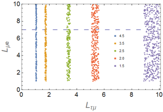
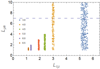
Figure 4: The dependence of $\triangle a_{\mu}$ (in unit of $10^{-10}$) on $L_{\mu e}$ and $L_{\tau\mu}$. The left(right) panel is for the NO(IO) benchmark point. The horizontal dash line represents the projected reach of MEGII[76], ${\cal B}(\mu\rightarrow e\gamma)<6\times 10^{-14}$ or $L_{\mu e}=7.0$.

We use the benchmark points to explore the dependence of $\triangle a_{\mu}$ on $L_{\mu e}$ and $L_{\tau\mu}$ by varying the $L$ values. From Fig.4, it is clear that $\triangle a_{\mu}$ is mainly controlled by $L_{\tau\mu}$, and $\triangle a_{\mu}\propto\sqrt{L_{\tau\mu}}$ as expected in Eq.(53). In some parameter space, as in the IO benchmark point, both $L_{\mu e}$ and $L_{\tau\mu}$ place comparable constraint on $\triangle a_{\mu}$. The projection limit on ${\cal B}(\tau\to\mu\gamma)$ by Belle II is $\sim 10^{-9}$[77], or $L_{\tau\mu}\sim 42$. If no CLFV $\tau\rightarrow\mu\gamma$ transition is observed before reaching that sensitivity, our model predicts $\triangle a_{\mu}\lesssim 1\times 10^{-10}$.

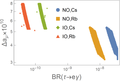
Figure 5: Correlation between ${\cal B}(\tau\to e\gamma)$ and $\Delta a_{\mu}$. The blue, orange, green, and red points stand for NO $\Delta a_{e}^{Cs}$, NO $\Delta a_{e}^{Rb}$, IO $\Delta a_{e}^{Cs}$, and NO$\Delta a_{e}^{Rb}$ respectively.

On the other hand, ${\cal B}(\tau\to e\gamma)$ can be much below the current limit, $<3.3\times 10^{-8}$[10], for IO while it is close to the current experimental constraint for NO. The numerical result, as shown in Fig.5, agrees with our naive expectation, Eq.(54), that ${\cal B}(\tau\to e\gamma)_{NO}>{\cal B}(\tau\to e\gamma)_{IO}$. Therefore, ${\cal B}(\tau\to e\gamma)$ could serve as an indirect probe to determine the type of neutrino mass hierarchy in our model.

In Fig.6, another observed correlation between $\triangle a_{\mu}$ and $\theta_{23}$ is displayed. This correlation can be understood as follows. Note that increasing $\theta_{23}$, while keeping all other neutrino oscillation parameters unchanged, results to a larger(smaller) $M^{\nu}_{22}$ for NO(IO) neutrino masses. On the other hand, since $M^{\nu}_{22}\propto(y^{L}_{2})^{2}$ and $\triangle a_{\mu}\propto y^{L}_{2}y^{R}_{2}$, the observed correlation follows.

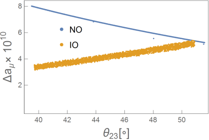
Figure 6: Correlation between $\theta_{23}$ and $\Delta a_{\mu}$. The blue(orange) dots stand for NO(IO) viable points.

Back to Fig.5, it is clear that ${\cal B}(\tau\to e\gamma)$ anti-correlates with $\triangle a_{\mu}$ for both neutrino mass hierarchy. It is because increasing $\theta_{23}$ leads to smaller(larger) $M^{\nu}_{33}$(thus $y^{L}_{3}$) for NO(IO). So together with the positive(negative) correlation between $\triangle a_{\mu}^{NO[IO]}$ and $\theta_{23}$, Fig.6, ${\cal B}(\tau\to e\gamma)\propto|y^{L}_{3}y^{R}_{1}|^{2}$ always anti-correlates with $\triangle a_{\mu}$.

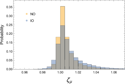
Figure 7: The probability histogram of the predicted normalized Higgs muon-Yukawa.

From all the viable points we found the effective muon-Higgs Yukawa coupling is close to the SM one. The range of the normalized muon-Yukawa, $\zeta_{\mu}$, is roughly between $0.98-1.05$. The distribution variance of IO is slightly larger than NO, but both peak at around $1.005$, as seen in Fig.7. It is well within the current $2\sigma$ constraint, $0.6\lesssim\zeta_{\mu}\lesssim 1.5$[6, 7]. For the future updates of $\zeta_{\mu}$[78], we also show the scatter plot of $\triangle a_{\mu}$ vs $\zeta_{\mu}$ in Fig.8. It is clear that $\zeta_{\mu}$ weakly correlates with $\triangle a_{\mu}$, and roughly half of the parameter space can be probed at the future FCC[79] with a projected precision of $\sim 0.4\%$ on muon-Yukawa.

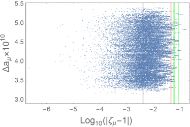
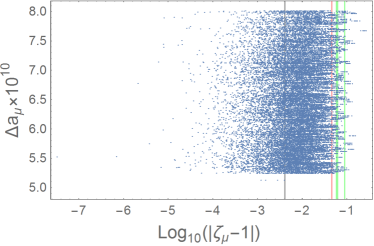
Figure 8: The left/right panel is the scatted plot of $\triangle a_{\mu}$ v.s. $\log_{10}(|\zeta_{\mu}-1|)$ for the NO/IO case. The vertical lines, from right to left, indicate the projected sensitivity[78] at CEPC[80], ILC[81]/CLIP[82], HL-HLC(red), and FCC[79](black), respectively.

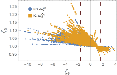
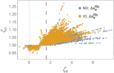
Figure 9: $\zeta_{e}$ v.s. $\zeta_{\mu}$. The vertical dashed lines indicate the projected sensitivity at FCC-ee[83].

Interestingly, this model predicts a possible unconventional electron-Higgs Yukawa coupling. This is due to $|\delta M_{ee}^{loop}|\gtrsim m_{e}$, and that can be traced back to the less constrained $y^{R}_{11,12}$. From Fig.9, it is clear that the magnitude of electron-Higgs Yukawa could be one order of magnitude larger than the SM prediction. The projected sensitivity, $|\zeta_{e}|<1.6$ at $95\%$ CL, at FCC-ee[83] is shown as the vertical dashed line. For the case of $\triangle a_{e}^{CS}$, the sign of electron-Higgs Yukawa could even be negative. However, the sign determination requires an interference with the tiny electron-Higgs Yukawa coupling, and thus very challenging in the foreseeable future.

In summary, from our numerical study, the viable model parameter space only requires (1) Majorana masses $\ll$ Dirac masses $\sim$ TeV, and (2) order $1(0.1)$ mixings among charged(neutral) scalars. Since we take a bottom-up approach, this model cannot address the pattern of neutrino mass matrix. It is taken as the experimental input. However, we find that the hierarchy among the model parameters $y^{L}$’s and $y^{R}$’s is less than 5 orders of magnitude for most of the cases. Thus, this model is technically natural, and no extreme fine-tuning is required to accommodate the neutrino oscillation data and $\triangle a_{e}^{Cs[Rb]}$.

IV Discussion and Phenomenology

SM Higgs decay

Due to the violation of lepton number, we also have $h_{SM}\rightarrow\nu_{i}\nu_{j}^{c}$ decays generated at one-loop level. By dimensional analysis, the effective $h_{SM}\mathchar 45\relax\nu_{i}\mathchar 45\relax\nu_{j}^{c}$ Yukawa coupling can be estimated to be $\sim\frac{1}{4\pi^{2}}\frac{m_{\nu}}{M}$, where $M$ is the typical mass of exotic degrees of freedom. The coupling strength is then $\sim{\cal O}(10^{-15})$ if taking $M\sim{\cal O}(1\mathrm{TeV})$, and being experimentally insignificant. Since we assume all the exotic DOF’s are heavier than $0.5\mathrm{TeV}$, there is no modification to the SM invisible Higgs decay width either. Because all new fields in our model are color singlet, the $ggh_{SM}$ vertex does not receive any correction at 1-loop level.

However, the two additional charged scalars contribute to di-photon Higgs decay width. The decay width is given by[84, 85]

$$\Gamma_{\gamma\gamma}={G_{F}\alpha_{em}^{2}M^{3}_{h_{SM}}\over 128\sqrt{2}\pi^{3}}\left|\frac{4}{3}F_{1/2}\left(\tau_{t}\right)+F_{1}(\tau_{W})+\sum_{a=1}^{2}\frac{v_{0}\widetilde{\mu}_{aa}}{2M_{C_{a}}^{2}}F_{0}(\tau_{C_{a}})\right|^{2}\,,$$ (56)

where $\widetilde{\mu}_{aa}$ is the charged scalar-Higgs cubic coupling given in Eq.(29). The $F_{1/2}$ and $F_{0}$ terms are the dominate SM 1-loop contributions from top quark and $W^{\pm}$ boson, respectively. We define $\tau_{i}=(M_{h_{SM}}/2M_{i})^{2}$, and the one-loop functions are given by

$$F_{0}(x)={f(x)-x\over x^{2}}\,,\;F_{1/2}(x)={2[x+(x-1)f(x)]\over x^{2}}\,,\;F_{1}(x)=-{2x^{2}+3x+3(2x-1)f(x)\over x^{2}}\,,$$ (57)

with $f(x)=[\arcsin(\sqrt{x})]^{2}$ for $x<1$. For $x\ll 1$, $F_{0}(x)\sim\frac{1}{3}+\frac{8}{45}x$. Plugging in the masses of top, $W^{\pm}$, and $h_{SM}$, we have $F_{1/2}\left(\tau_{t}\right)=1.38$ and $F_{1}(\tau_{W})=-8.32$. Assuming that $\mu_{DC}\gg v_{0}$, we have approximately $\widetilde{\mu}_{11}\sim-2s_{\alpha}c_{\alpha}\mu_{DC}$ and $\widetilde{\mu}_{22}\sim+2s_{\alpha}c_{\alpha}\mu_{DC}$. So the width becomes

$$\Gamma_{\gamma\gamma}\simeq{G_{F}\alpha_{em}^{2}M^{3}_{h_{SM}}\over 128\sqrt{2}\pi^{3}}\left|(-6.49)_{SM}-\frac{1}{3}\left({v_{0}\mu_{DC}\over M_{C_{1}}M_{C_{2}}}\right)^{2}\right|^{2}\,.$$ (58)

It is clear that $\Gamma_{\gamma\gamma}/\Gamma^{SM}_{\gamma\gamma}>1$. Assuming $M_{C_{1}}=0.5\mathrm{TeV}$ and $\mu_{DC}\simeq M_{C_{2}}$, then the NP will only modify the di-photon decay width by a magnitude $\sim 2\%$. Comparing to the latest coupling scaling factor $\kappa_{\gamma}=1.06\pm 0.05$ obtained by [86], we expect a weak constraint on this model from the Higgs diphoton decay.

CLFV $\mu\rightarrow e$ conversion, and $\mu\rightarrow 3e$

Concerning on the other CLFV experimental bounds on the model parameter space, we comment on the $\mu\mathchar 45\relax e$ conversion on nuclei and $\mu\rightarrow 3e$.

For $\mu\mathchar 45\relax e$ conversion on nuclei, the current upper bound of the ratio of $\mu\rightarrow e$ conversion rate normalized to the muon capture rate[87],

$$R_{\mu e}={\Gamma(\mu+(A,Z)\rightarrow e+(A,Z))\over\Gamma(\mu+(A,Z)\rightarrow\nu_{\mu}+(A,Z-1))}<7\times 10^{-13}\,,$$ (59)

is given by SINDRUM II with gold as target[88]. Since the hidden sector does not couple to the SM quark sector, the $\mu\rightarrow e$ conversion is dominated by the $\mu e\gamma$ dipole. For a given target nuclei $N$, the $\mu\rightarrow e$ conversion rate can be expressed as

$$\Gamma_{\mu\rightarrow e}\sim\pi D_{N}^{2}\Gamma_{\mu}{\cal B}(\mu\rightarrow e\gamma)\,,$$ (60)

where $\Gamma_{\mu}=0.45517\times 10^{6}s^{-1}$[10] is the muon decay rate, and $D_{N}$ is the lepton-nucleus overlap integral coefficient. For gold and aluminum, $D_{Au}=0.189$ and $D_{Al}=0.0362$ [89], while the muon capture rates are $13.07\times 10^{6}s^{-1}$ and $0.71\times 10^{6}s^{-1}$, respectively[89, 90]. Plugging in the values of $\Gamma_{\mu}$ and the current upper limit of ${\cal B}(\mu\rightarrow e\gamma)$, one finds $R_{\mu e}<10^{-15}$ with Au or Al target, roughly three orders of magnitude below the current experimental limit. In the near future, the model prediction, Eq.(60), could be checked with improved sensitivity[91, 92, 93, 94].

Figure 10: The box diagram for $\mu\rightarrow 3e$ transition, where $a,b\in\{1,2\}$ and $i,j\in\{1,2,3,4\}$.

In this model, $\mu\rightarrow 3e$ can be induced by the CLFV $\mu e\gamma$ dipole coupling and the box diagram shown in Fig.10. The contribution form the $\mu e\gamma$ dipole can be calculated to be[95, 87, 73]

$$\Gamma(\mu\rightarrow 3e)_{dip}\simeq\frac{2\alpha_{em}}{3\pi}\left[\ln\frac{m_{\mu}}{m_{e}}-\frac{11}{8}\right]\Gamma(\mu\rightarrow e\gamma)\,.$$ (61)

This part is about three orders of magnitude below the current bound of ${\cal B}(\mu\rightarrow 3e)<10^{-12}$[96]. In addition to the dipole contribution, the box-diagram gives rise to FCNC 4-fermi interactions[73]:

$${\cal L}\supset-\frac{4G_{F}}{\sqrt{2}}\left[g_{1}\left(\bar{e}\hat{L}\mu\right)\left(\bar{e}\hat{L}e\right)+g_{3}\left(\bar{e}\gamma^{\alpha}\hat{R}\mu\right)\left(\bar{e}\gamma_{\alpha}\hat{R}e\right)+g_{5}\left(\bar{e}\gamma^{\alpha}\hat{R}\mu\right)\left(\bar{e}\gamma_{\alpha}\hat{L}e\right)+(\hat{L}\Leftrightarrow\hat{R})\right]+H.c.\,,$$ (62)

and leads to

$${\cal B}(\mu\rightarrow 3e)_{4fermi}\simeq\frac{|g_{1}|^{2}}{8}+2|g_{3}|^{2}+|g_{5}|^{2}+(\hat{L}\Leftrightarrow\hat{R})\,,$$ (63)

if ignoring the interference between the dipole and 4-fermi interactions. By dimension analysis, the dimensionless Wilson coefficients can be estimated as

$$|g|\sim\frac{1}{16\pi^{2}}\frac{\sqrt{2}}{4G_{F}}{Y_{e}^{3}Y_{\mu}\over M^{2}}\times(0.5)\,,$$ (64)

where $M$ is the relevant highest mass in the loop, $0.5$ is the typical value from the box-diagram loop integration, and $Y_{e}^{3}Y_{\mu}$ denotes the product of four relevant LH or RH Yukawa couplings. Thus, ${\cal B}(\mu\rightarrow 3e)_{4fermi}\simeq 10^{-15}(2\mathrm{TeV}/M)^{4}(Y_{e}^{3}Y_{\mu}/0.001)^{2}$ is also expected to be safely below the current experimental limit. The $\mu\rightarrow 3e$ decay could be a relevant constraint and probed by the planned Mu3e experiment with a sensitivity of $10^{-16}$[97] in the near future. For CLFV $\tau\rightarrow l_{i}l_{j}l_{k}\,(l_{i,j,k}=e,\mu)$ decay branching ratios, the current bounds, $(\mbox{a few})\times 10^{-8}$[98], and the future $\sim 10^{-10}$ sensitivity [77, 99, 100] do not post further constraint on this model.

$Z_{X}$: The smoking gun of the gauge $U(1)_{X}$

One robust prediction of gauge $U(1)_{X}$ is the existence of the gauge boson, $Z_{X}$. The direct detection of $Z_{X}$ will be the smoking gun of the gauge $U(1)_{X}$. Here we give a brief remark on the prospects on its discovery. As discussed earlier, after $S_{2}$ acquires a VEV $v_{2}$, $Z_{X}$ also acquires a mass $M_{Z_{X}}=2g_{X}v_{2}$. But $Z_{X}$ does not play any role in our flavor physics discussion. So far, both the gauge coupling $g_{X}$ and $M_{Z_{X}}$ are unknown free parameters. Although $Z_{X}$ does not couple to any of the SM fields at tree-level, its couplings to $\gamma Z,ZZ,W^{+}W^{-},h_{SM}h_{SM},\gamma h_{SM},Zh_{SM}$, and lepton pairs can be generated at one-loop level. Also, the one-loop vacuum polarization diagrams can generate the $Z_{X}\mathchar 45\relax Z$ and $Z_{X}\mathchar 45\relax\gamma$ mixings. The $Z_{X}\mathchar 45\relax Z$ and $Z_{X}\mathchar 45\relax\gamma$ mixings can also be induced through the tree-level kinematic mixing between the field strengthes of $U(1)_{X}$ and $U(1)_{Y}$, ${\cal L}\supset-\frac{\epsilon}{2}B^{\mu\nu}X_{\mu\nu}$, see [101, 102, 103]. Since the kinematic mixing term is gauge invariant and renormalizable, $\epsilon$ is not required to be small. The kinematic mixing term can be rotated away by a $GL(2)$ transformation, and the two massive eigenstates couple to SM fields. From electroweak precision measurements, $h_{SM}\rightarrow ZZ_{X}$, and the Drell-Yan process, the mixing is constrained to be $\epsilon\lesssim 10^{-2}$ for $10\,\mathrm{GeV}\lesssim M_{Z_{X}}\lesssim 1\,\mathrm{TeV}$[104]. In the future, the HL-LHC and HE-LHC can probe the effective mixing to the level about $\sim 10^{-3}$ for $10\,\mathrm{GeV}\lesssim M_{Z_{X}}\lesssim 90\,\mathrm{GeV}$ and $0.2\,\mathrm{TeV}\lesssim M_{Z_{X}}\lesssim 2\,\mathrm{TeV}$[104]. In this model, the $\epsilon$ parameter is the combination of tree-level and 1-loop contributions. Moreover, the $Z_{X}$ to lepton pair couplings receive flavor dependent quantum corrections. At the LHC, the Drell-Yan processes $pp\rightarrow Z^{*}\rightarrow ZZ_{X}$, or $pp\rightarrow W^{*}\rightarrow WZ_{X}$ will be the dominate $Z_{X}$ production mechanism for $M_{Z_{X}}\gtrsim 180\,\mathrm{GeV}$. And the decays $Z_{X}\rightarrow l_{i}^{+}l_{j}^{-}$ with di-lepton invariant mass peaked at around $m_{l_{i}l_{j}}\simeq M_{Z_{X}}$ will be the clear signal. Incidentally, in this model the CLFV di-lepton decay connects to the flavor physics that we have discussed. A comprehensive study on this topic is beyond the scope of this paper, and we will leave it to the future works.

Dark matter

Finally, we give a sketchy discussion on DM in this model. After the SSB of $U(1)_{X}$ by $S_{2}$, the remaining gauge discrete parity[43] stabilizes the the lightest neutral DOF carrying one unit of $U(1)_{X}$ charge. Apparently, this DOF is a DM candidate. There are two possible candidates in our model: (1) $S_{D}$, the lighter of $R_{1}$ and $I_{1}$, and (2) $\chi_{4}$, the lightest mass eigenstate of the exotic fermions. From our numerical scan, about $\sim 70(30)\%$ of the solutions yield scalar(fermionic) DM candidate. And about $\sim 90\%$ of the potential DM mass is in the range of $[0.5,1.0]\mathrm{TeV}$. For a DM in that mass range, the current observational upper limits on the spin-independent DM-nucleon cross section is $\sigma_{SI}\lesssim 10^{-46}(cm)^{2}$ [105, 106, 107]. In our model, both $S_{D}$ and $\chi_{4}$ do not couple to the SM quark sector at tree-level and all the new DOFs are color singlets. Hence, for both DM candidates the $\sigma_{SI}$ can be easily arranged to stay below the direct detection bounds.

If $\chi_{4}$ is the DM candidate, the relic density is determined mainly by $t$- and $u$-channel annihilation $\chi_{4}\chi_{4}\rightarrow l\bar{l}(l=l^{-},\nu)$, and the $s-$channel $\chi_{4}\chi_{4}\rightarrow h_{2}\,\mbox{or}\,h_{SM}\rightarrow(SM)(SM)$ processes, where $(SM)$ stands for any SM field coupled to the SM Higgs. On the other hand, for the bosonic DM case, the relic density is mainly controlled by the $S_{D}S_{D}\rightarrow h_{SM}h_{SM}$, $S_{D}S_{D}\rightarrow h_{2}\,\mbox{or}\,h_{SM}\rightarrow(SM)(SM)$, and $S_{D}S_{D}\rightarrow W^{+}W^{-},ZZ$. One needs to take into account the co-annihilation $R_{1}I_{1}\rightarrow(SM)(SM)$ when $R_{1}$ and $I_{1}$ are nearly degenerate.

It should be emphasised that although the DM candidate is stable, phenomenology only demands that its relic density must not exceed the observed DM relic density, $\Omega_{DM}h^{2}=0.120\pm 0.001$[108]. However, the full evaluation of the relic density requires more model parameters which are independent of the flavor physics we are focusing on, and the comprehensive analysis of the extended parameter space is beyond the scope of this paper.

V Conclusion

Motivated by the recently measured anomalous magnetic moments of muon and electron, we studied a model with gauge hidden $U(1)_{X}$ symmetry as the unified framework to accommodate both the radiative neutrino mass generation mechanism and the measured $\triangle a_{\mu,e}$. This UV-complete model employs four exotic scalars and a minimum of two pairs of exotic vector fermions, all charged under $U(1)_{X}$, as seen in Table-1. The $U(1)_{X}$ is assumed to be spontaneously broken at an energy scale higher then the SM electroweak scale when one of the exotic singlet bosons gets a non-zero VEV. After the SSB of $U(1)_{X}$, the new fermions acquire Majorana masses, which are crucial to the radiative neutrino mass generation. Moreover, the new vector fermions admit tree-level Dirac masses which are essential for chirality flipping in explaining $\triangle a_{l}$.

Any mechanism that gives rise to charged lepton anomalous magnetic moments could potentially lead to CLFV which are stringently constrained by experiments. Usually, additional flavor symmetries or assumptions are summoned to suppress the unwanted CLFV. Contrarily, in this work we took a bottom-up approach and asked what restrictions the experimental constraints would impose upon the model parameter space. We have carefully taken into account the neutrino oscillation data and the experimental CLFV limits in our numerical study. We found that the model can explain the observed neutrino oscillation data, either normal or inverted ordering, and the central value of $\triangle a_{e}^{Cs[Rb]}$ without much fine-tuning on the model parameters. However, in the minimal model, the current experimental CLFV limit on ${\cal B}(\tau\rightarrow\mu\gamma)<4.4\times 10^{-8}$[75] results in $\triangle a_{\mu}\sim(4-8)\times 10^{-10}$, which differs from $\triangle a_{\mu}^{F\!N\!A\!L}\simeq(25.1\pm 5.9)\times 10^{-10}$[20] by $\sim 3\sigma$’s, but agrees with the SM prediction using the recent lattice QCD evaluation on hardronic contribution to $a_{\mu}$[22, 23]. Of course, more theoretical and experimental investigations are needed to settle down the $\triangle a_{\mu}$ issue. We pointed out that the future improvement on the CLFV limit will further suppress our predicted $\triangle a_{\mu}$ because of $(\triangle a_{\mu})^{2}\propto{\cal B}(\tau\rightarrow\mu\gamma)$ in our model.

The unconventional electron-Higgs Yukawa is another intriguing feature of this model. We found that the magnitude of electron-Higgs Yukawa can be one order of magnitude larger than the SM prediction. This unusual electron Yukawa can be probed at the future FCC-ee[83]. More interestingly, if $\triangle a_{e}^{Cs}$ is confirmed in the future, a negative electron-Higgs Yukawa could be allowed in this model. Due to the smallness of electron-Higgs Yukawa, the determination of its sign is extremely challenging in the foreseeable future. On the other hand, the muon-Higgs Yukawa is found to be close to the SM prediction with the deviation fraction $\lesssim 10^{-2}$ for most of the viable model parameter space. Although the deviation of muon-Higgs Yukawa is small, it could be probed at the FCC with a projected precision of $\sim 0.4\%$[78].

Since our approach is bottom-up, the prediction $\triangle a_{\mu}<\triangle a_{\mu}^{F\!N\!A\!L}$ is robust and applies to the minimal model with arbitrary add-on flavor symmetry. One has to go beyond the minimal model if the deviation between the experimentally and theoretically improved $\triangle a_{\mu}$ and the model prediction persists, or a few$\times 10\%$ muon Yukawa deviation is confirmed in the future. If that is the case, a trivial extension of this model by utilizing the third pair of vector fermion will do the job, and an even more enormous electron-Higgs Yukawa coupling strength is possible.

From the exercise, we have demonstrated that due to the smallness of the SM electron Yukawa, the effective electron-Higgs coupling strength is sensitive to new physics and plays a vital role in testing our understanding of flavor physics.

References

- Aaboud et al. [2018a] M. Aaboud et al. (ATLAS), Measurements of Higgs boson properties in the diphoton decay channel with 36 fb-1 of collision data at TeV with the ATLAS detector, Phys. Rev. D 98, 052005 (2018a), arXiv:1802.04146 [hep-ex] .
- Aaboud et al. [2018b] M. Aaboud et al. (ATLAS), Observation of decays and production with the ATLAS detector, Phys. Lett. B 786, 59 (2018b), arXiv:1808.08238 [hep-ex] .
- Sirunyan et al. [2018a] A. M. Sirunyan et al. (CMS), Observation of Higgs boson decay to bottom quarks, Phys. Rev. Lett. 121, 121801 (2018a), arXiv:1808.08242 [hep-ex] .
- Aad et al. [2015] G. Aad et al. (ATLAS), Evidence for the Higgs-boson Yukawa coupling to tau leptons with the ATLAS detector, JHEP 04, 117, arXiv:1501.04943 [hep-ex] .
- Sirunyan et al. [2018b] A. M. Sirunyan et al. (CMS), Observation of the Higgs boson decay to a pair of leptons with the CMS detector, Phys. Lett. B 779, 283 (2018b), arXiv:1708.00373 [hep-ex] .
- Aad et al. [2021] G. Aad et al. (ATLAS), A search for the dimuon decay of the Standard Model Higgs boson with the ATLAS detector, Phys. Lett. B 812, 135980 (2021), arXiv:2007.07830 [hep-ex] .
- Sirunyan et al. [2021] A. M. Sirunyan et al. (CMS), Evidence for Higgs boson decay to a pair of muons, JHEP 01, 148, arXiv:2009.04363 [hep-ex] .
- Aad et al. [2020a] G. Aad et al. (ATLAS), Combined measurements of Higgs boson production and decay using up to fb-1 of proton-proton collision data at 13 TeV collected with the ATLAS experiment, Phys. Rev. D 101, 012002 (2020a), arXiv:1909.02845 [hep-ex] .
- Sirunyan et al. [2019] A. M. Sirunyan et al. (CMS), Combined measurements of Higgs boson couplings in proton–proton collisions at , Eur. Phys. J. C 79, 421 (2019), arXiv:1809.10733 [hep-ex] .
- Zyla et al. [2020] P. A. Zyla et al. (Particle Data Group), Review of Particle Physics, PTEP 2020, 083C01 (2020).
- Khachatryan et al. [2015] V. Khachatryan et al. (CMS), Search for a standard model-like Higgs boson in the and decay channels at the LHC, Phys. Lett. B 744, 184 (2015), arXiv:1410.6679 [hep-ex] .
- Aad et al. [2020b] G. Aad et al. (ATLAS), Search for the Higgs boson decays and in collisions at TeV with the ATLAS detector, Phys. Lett. B 801, 135148 (2020b), arXiv:1909.10235 [hep-ex] .
- Botella et al. [2016] F. J. Botella, G. C. Branco, M. N. Rebelo, and J. I. Silva-Marcos, What if the masses of the first two quark families are not generated by the standard model Higgs boson?, Phys. Rev. D 94, 115031 (2016), arXiv:1602.08011 [hep-ph] .
- Ghosh et al. [2016] D. Ghosh, R. S. Gupta, and G. Perez, Is the Higgs Mechanism of Fermion Mass Generation a Fact? A Yukawa-less First-Two-Generation Model, Phys. Lett. B 755, 504 (2016), arXiv:1508.01501 [hep-ph] .
- Altmannshofer et al. [2016] W. Altmannshofer, S. Gori, A. L. Kagan, L. Silvestrini, and J. Zupan, Uncovering Mass Generation Through Higgs Flavor Violation, Phys. Rev. D 93, 031301 (2016), arXiv:1507.07927 [hep-ph] .
- Dery et al. [2018] A. Dery, C. Frugiuele, and Y. Nir, Large Higgs-electron Yukawa coupling in 2HDM, JHEP 04, 044, arXiv:1712.04514 [hep-ph] .
- Chiang and Yagyu [2021] C.-W. Chiang and K. Yagyu, Radiative Seesaw Mechanism for Charged Leptons, Phys. Rev. D 103, L111302 (2021), arXiv:2104.00890 [hep-ph] .
- Esteban et al. [2020] I. Esteban, M. C. Gonzalez-Garcia, M. Maltoni, T. Schwetz, and A. Zhou, The fate of hints: updated global analysis of three-flavor neutrino oscillations, JHEP 09, 178, arXiv:2007.14792 [hep-ph] .
- Aoyama et al. [2020] T. Aoyama et al., The anomalous magnetic moment of the muon in the Standard Model, Phys. Rept. 887, 1 (2020), arXiv:2006.04822 [hep-ph] .
- Abi et al. [2021] B. Abi et al. (Muon g-2), Measurement of the Positive Muon Anomalous Magnetic Moment to 0.46 ppm, Phys. Rev. Lett. 126, 141801 (2021), arXiv:2104.03281 [hep-ex] .
- Saito [2012] N. Saito (J-PARC g-’2/EDM), A novel precision measurement of muon g-2 and EDM at J-PARC, AIP Conf. Proc. 1467, 45 (2012).
- Borsanyi et al. [2021] S. Borsanyi et al., Leading hadronic contribution to the muon magnetic moment from lattice QCD, Nature 593, 51 (2021), arXiv:2002.12347 [hep-lat] .
- Cè et al. [2022] M. Cè et al., Window observable for the hadronic vacuum polarization contribution to the muon from lattice QCD, (2022), arXiv:2206.06582 [hep-lat] .
- Crivellin et al. [2020] A. Crivellin, M. Hoferichter, C. A. Manzari, and M. Montull, Hadronic Vacuum Polarization: versus Global Electroweak Fits, Phys. Rev. Lett. 125, 091801 (2020), arXiv:2003.04886 [hep-ph] .
- Keshavarzi et al. [2020] A. Keshavarzi, W. J. Marciano, M. Passera, and A. Sirlin, Muon and connection, Phys. Rev. D 102, 033002 (2020), arXiv:2006.12666 [hep-ph] .
- Colangelo et al. [2021] G. Colangelo, M. Hoferichter, and P. Stoffer, Constraints on the two-pion contribution to hadronic vacuum polarization, Phys. Lett. B 814, 136073 (2021), arXiv:2010.07943 [hep-ph] .
- Parker et al. [2018] R. H. Parker, C. Yu, W. Zhong, B. Estey, and H. Müller, Measurement of the fine-structure constant as a test of the Standard Model, Science 360, 191 (2018), arXiv:1812.04130 [physics.atom-ph] .
- Morel et al. [2020] L. Morel, Z. Yao, P. Cladé, and S. Guellati-Khélifa, Determination of the fine-structure constant with an accuracy of 81 parts per trillion, Nature 588, 61 (2020).
- Abdullah et al. [2019] M. Abdullah, B. Dutta, S. Ghosh, and T. Li, and the ANITA anomalous events in a three-loop neutrino mass model, Phys. Rev. D 100, 115006 (2019), arXiv:1907.08109 [hep-ph] .
- Chen and Nomura [2021] C.-H. Chen and T. Nomura, Electron and muon , radiative neutrino mass, and in a model, Nucl. Phys. B 964, 115314 (2021), arXiv:2003.07638 [hep-ph] .
- Dutta et al. [2020] B. Dutta, S. Ghosh, and T. Li, Explaining , the KOTO anomaly and the MiniBooNE excess in an extended Higgs model with sterile neutrinos, Phys. Rev. D 102, 055017 (2020), arXiv:2006.01319 [hep-ph] .
- Arbeláez et al. [2020] C. Arbeláez, R. Cepedello, R. M. Fonseca, and M. Hirsch, anomalies and neutrino mass, Phys. Rev. D 102, 075005 (2020), arXiv:2007.11007 [hep-ph] .
- Jana et al. [2020a] S. Jana, P. K. Vishnu, W. Rodejohann, and S. Saad, Dark matter assisted lepton anomalous magnetic moments and neutrino masses, Phys. Rev. D 102, 075003 (2020a), arXiv:2008.02377 [hep-ph] .
- Cao et al. [2021] J. Cao, Y. He, J. Lian, D. Zhang, and P. Zhu, Electron and muon anomalous magnetic moments in the inverse seesaw extended NMSSM, Phys. Rev. D 104, 055009 (2021), arXiv:2102.11355 [hep-ph] .
- Mondal and Okada [2022] T. Mondal and H. Okada, Inverse seesaw and (g-2) anomalies in B-L extended two Higgs doublet model, Nucl. Phys. B 976, 115716 (2022), arXiv:2103.13149 [hep-ph] .
- Escribano et al. [2021] P. Escribano, J. Terol-Calvo, and A. Vicente, in an extended inverse type-III seesaw model, Phys. Rev. D 103, 115018 (2021), arXiv:2104.03705 [hep-ph] .
- Hernández et al. [2021] A. E. C. Hernández, S. Kovalenko, M. Maniatis, and I. Schmidt, Fermion mass hierarchy and g 2 anomalies in an extended 3HDM Model, JHEP 10, 036, arXiv:2104.07047 [hep-ph] .
- Chang [2021] W.-F. Chang, One colorful resolution to the neutrino mass generation, three lepton flavor universality anomalies, and the Cabibbo angle anomaly, (2021), arXiv:2105.06917 [hep-ph] .
- Borah et al. [2022] D. Borah, M. Dutta, S. Mahapatra, and N. Sahu, Lepton anomalous magnetic moment with singlet-doublet fermion dark matter in a scotogenic U(1)L-L model, Phys. Rev. D 105, 015029 (2022), arXiv:2109.02699 [hep-ph] .
- Julio et al. [2022a] J. Julio, S. Saad, and A. Thapa, A Tale of Flavor Anomalies and the Origin of Neutrino Mass, (2022a), arXiv:2202.10479 [hep-ph] .
- Julio et al. [2022b] J. Julio, S. Saad, and A. Thapa, Marriage between neutrino mass and flavor anomalies, (2022b), arXiv:2203.15499 [hep-ph] .
- Chowdhury et al. [2022] T. A. Chowdhury, M. Ehsanuzzaman, and S. Saad, Dark Matter and in radiative Dirac neutrino mass models, (2022), arXiv:2203.14983 [hep-ph] .
- Krauss and Wilczek [1989] L. M. Krauss and F. Wilczek, Discrete Gauge Symmetry in Continuum Theories, Phys. Rev. Lett. 62, 1221 (1989).
- Gu and Sarkar [2008] P.-H. Gu and U. Sarkar, Radiative Neutrino Mass, Dark Matter and Leptogenesis, Phys. Rev. D 77, 105031 (2008), arXiv:0712.2933 [hep-ph] .
- Ma et al. [2013] E. Ma, I. Picek, and B. Radovčić, New Scotogenic Model of Neutrino Mass with Gauge Interaction, Phys. Lett. B 726, 744 (2013), arXiv:1308.5313 [hep-ph] .
- Kanemura et al. [2011] S. Kanemura, O. Seto, and T. Shimomura, Masses of dark matter and neutrino from TeV scale spontaneous breaking, Phys. Rev. D 84, 016004 (2011), arXiv:1101.5713 [hep-ph] .
- Chang and Wong [2012] W.-F. Chang and C.-F. Wong, A Model for Neutrino Masses and Dark Matter with the Discrete Gauge Symmetry, Phys. Rev. D 85, 013018 (2012), arXiv:1104.3934 [hep-ph] .
- Baek [2016] S. Baek, Dark matter and muon in local -extended Ma Model, Phys. Lett. B 756, 1 (2016), arXiv:1510.02168 [hep-ph] .
- Ho et al. [2016] S.-Y. Ho, T. Toma, and K. Tsumura, Systematic extensions of loop-induced neutrino mass models with dark matter, Phys. Rev. D 94, 033007 (2016), arXiv:1604.07894 [hep-ph] .
- Ma et al. [2016] E. Ma, N. Pollard, O. Popov, and M. Zakeri, Gauge model of radiative neutrino mass with multipartite dark matter, Mod. Phys. Lett. A 31, 1650163 (2016), arXiv:1605.00991 [hep-ph] .
- Nomura and Okada [2019] T. Nomura and H. Okada, Radiative neutrino mass in an alternative gauge symmetry, Nucl. Phys. B 941, 586 (2019), arXiv:1705.08309 [hep-ph] .
- Geng and Okada [2018] C.-Q. Geng and H. Okada, Neutrino masses, dark matter and leptogenesis with gauge symmetry, Phys. Dark Univ. 20, 13 (2018), arXiv:1710.09536 [hep-ph] .
- Han and Wang [2018] Z.-L. Han and W. Wang, Portal Dark Matter in Scotogenic Dirac Model, Eur. Phys. J. C 78, 839 (2018), arXiv:1805.02025 [hep-ph] .
- Centelles Chuliá et al. [2020] S. Centelles Chuliá, R. Cepedello, E. Peinado, and R. Srivastava, Scotogenic dark symmetry as a residual subgroup of Standard Model symmetries, Chin. Phys. C 44, 083110 (2020), arXiv:1901.06402 [hep-ph] .
- Ma [2019a] E. Ma, Scotogenic Dirac neutrinos, Phys. Lett. B 793, 411 (2019a), arXiv:1901.09091 [hep-ph] .
- Kang et al. [2019] S. K. Kang, O. Popov, R. Srivastava, J. W. F. Valle, and C. A. Vaquera-Araujo, Scotogenic dark matter stability from gauged matter parity, Phys. Lett. B 798, 135013 (2019), arXiv:1902.05966 [hep-ph] .
- Jana et al. [2019] S. Jana, P. K. Vishnu, and S. Saad, Minimal dirac neutrino mass models from gauge symmetry and left–right asymmetry at colliders, Eur. Phys. J. C 79, 916 (2019), arXiv:1904.07407 [hep-ph] .
- Ma [2019b] E. Ma, Scotogenic cobimaximal Dirac neutrino mixing from and , Eur. Phys. J. C 79, 903 (2019b), arXiv:1905.01535 [hep-ph] .
- Centelles Chuliá et al. [2019] S. Centelles Chuliá, R. Cepedello, E. Peinado, and R. Srivastava, Systematic classification of two loop = 4 Dirac neutrino mass models and the Diracness-dark matter stability connection, JHEP 10, 093, arXiv:1907.08630 [hep-ph] .
- Jana et al. [2020b] S. Jana, P. K. Vishnu, and S. Saad, Minimal realizations of Dirac neutrino mass from generic one-loop and two-loop topologies at , JCAP 04, 018, arXiv:1910.09537 [hep-ph] .
- de la Vega et al. [2020] L. M. G. de la Vega, N. Nath, and E. Peinado, Dirac neutrinos from Peccei-Quinn symmetry: two examples, Nucl. Phys. B 957, 115099 (2020), arXiv:2001.01846 [hep-ph] .
- Wong [2021] C.-F. Wong, Anomaly-free chiral and its scotogenic implication, Phys. Dark Univ. 32, 100818 (2021), arXiv:2008.08573 [hep-ph] .
- Chao [2011] W. Chao, Pure Leptonic Gauge Symmetry, Neutrino Masses and Dark Matter, Phys. Lett. B 695, 157 (2011), arXiv:1005.1024 [hep-ph] .
- Schwaller et al. [2013] P. Schwaller, T. M. P. Tait, and R. Vega-Morales, Dark Matter and Vectorlike Leptons from Gauged Lepton Number, Phys. Rev. D 88, 035001 (2013), arXiv:1305.1108 [hep-ph] .
- Chang and Ng [2018a] W.-F. Chang and J. N. Ng, Study of Gauged Lepton Symmetry Signatures at Colliders, Phys. Rev. D 98, 035015 (2018a), arXiv:1805.10382 [hep-ph] .
- Chang and Ng [2018b] W.-F. Chang and J. N. Ng, Neutrino masses and gauged lepton number, JHEP 10, 015, arXiv:1807.09439 [hep-ph] .
- Chang and Ng [2019] W.-F. Chang and J. N. Ng, Alternative Perspective on Gauged Lepton Number and Implications for Collider Physics, Phys. Rev. D 99, 075025 (2019), arXiv:1808.08188 [hep-ph] .
- Chang and Ng [2014] W.-F. Chang and J. N. Ng, Minimal model of Majoronic dark radiation and dark matter, Phys. Rev. D 90, 065034 (2014), arXiv:1406.4601 [hep-ph] .
- Chang and Ng [2016] W.-F. Chang and J. N. Ng, Renormalization Group Study of the Minimal Majoronic Dark Radiation and Dark Matter Model, JCAP 07, 027, arXiv:1604.02017 [hep-ph] .
- CMS [2020] Combined Higgs boson production and decay measurements with up to 137 fb-1 of proton-proton collision data at = 13 TeV, CMS-PAS-HIG-19-005, (2020).
- ATL [2021] Combined measurements of Higgs boson production and decay using up to fb-1 of proton-proton collision data at TeV collected with the ATLAS experiment, ATLAS-CONF-2021-053, (2021).
- Barlow [2004] R. Barlow, Asymmetric statistical errors, in Statistical Problems in Particle Physics, Astrophysics and Cosmology (2004) pp. 56–59, arXiv:physics/0406120 .
- Chang and Ng [2005] W.-F. Chang and J. N. Ng, Lepton flavor violation in extra dimension models, Phys. Rev. D 71, 053003 (2005), arXiv:hep-ph/0501161 .
- Baldini et al. [2016] A. M. Baldini et al. (MEG), Search for the lepton flavour violating decay with the full dataset of the MEG experiment, Eur. Phys. J. C 76, 434 (2016), arXiv:1605.05081 [hep-ex] .
- Aubert et al. [2010] B. Aubert et al. (BaBar), Searches for Lepton Flavor Violation in the Decays tau+- — e+- gamma and tau+- — mu+- gamma, Phys. Rev. Lett. 104, 021802 (2010), arXiv:0908.2381 [hep-ex] .
- Baldini et al. [2018] A. M. Baldini et al. (MEG II), The design of the MEG II experiment, Eur. Phys. J. C 78, 380 (2018), arXiv:1801.04688 [physics.ins-det] .
- Altmannshofer et al. [2019] W. Altmannshofer et al. (Belle-II), The Belle II Physics Book, PTEP 2019, 123C01 (2019), [Erratum: PTEP 2020, 029201 (2020)], arXiv:1808.10567 [hep-ex] .
- de Blas et al. [2020] J. de Blas et al., Higgs Boson Studies at Future Particle Colliders, JHEP 01, 139, arXiv:1905.03764 [hep-ph] .
- Abada et al. [2019] A. Abada et al. (FCC), FCC Physics Opportunities: Future Circular Collider Conceptual Design Report Volume 1, Eur. Phys. J. C 79, 474 (2019).
- Dong et al. [2018] M. Dong et al. (CEPC Study Group), CEPC Conceptual Design Report: Volume 2 - Physics & Detector, (2018), arXiv:1811.10545 [hep-ex] .
- Bambade et al. [2019] P. Bambade et al., The International Linear Collider: A Global Project, (2019), arXiv:1903.01629 [hep-ex] .
- Charles et al. [2018] T. K. Charles et al. (CLICdp, CLIC), The Compact Linear Collider (CLIC) - 2018 Summary Report 2/2018, 10.23731/CYRM-2018-002 (2018), arXiv:1812.06018 [physics.acc-ph] .
- d’Enterria et al. [2022] D. d’Enterria, A. Poldaru, and G. Wojcik, Measuring the electron Yukawa coupling via resonant s-channel Higgs production at FCC-ee, Eur. Phys. J. Plus 137, 201 (2022), arXiv:2107.02686 [hep-ex] .
- Shifman et al. [1979] M. A. Shifman, A. I. Vainshtein, M. B. Voloshin, and V. I. Zakharov, Low-Energy Theorems for Higgs Boson Couplings to Photons, Sov. J. Nucl. Phys. 30, 711 (1979).
- Chang et al. [2012] W.-F. Chang, J. N. Ng, and J. M. S. Wu, Constraints on New Scalars from the LHC 125 GeV Higgs Signal, Phys. Rev. D 86, 033003 (2012), arXiv:1206.5047 [hep-ph] .
- ATL [2020] A combination of measurements of Higgs boson production and decay using up to fb-1 of proton–proton collision data at 13 TeV collected with the ATLAS experiment, ATLAS-CONF-2020-027, (2020).
- Kuno and Okada [2001] Y. Kuno and Y. Okada, Muon decay and physics beyond the standard model, Rev. Mod. Phys. 73, 151 (2001), arXiv:hep-ph/9909265 .
- Bertl et al. [2006] W. H. Bertl et al. (SINDRUM II), A Search for muon to electron conversion in muonic gold, Eur. Phys. J. C 47, 337 (2006).
- Kitano et al. [2002] R. Kitano, M. Koike, and Y. Okada, Detailed calculation of lepton flavor violating muon electron conversion rate for various nuclei, Phys. Rev. D 66, 096002 (2002), [Erratum: Phys.Rev.D 76, 059902 (2007)], arXiv:hep-ph/0203110 .
- Suzuki et al. [1987] T. Suzuki, D. F. Measday, and J. P. Roalsvig, Total Nuclear Capture Rates for Negative Muons, Phys. Rev. C 35, 2212 (1987).
- Teshima [2018] N. Teshima (DeeMe), DeeMe experiment to search for muon to electron conversion at J-PARC MLF, PoS NuFact2017, 109 (2018).
- Abramishvili et al. [2020] R. Abramishvili et al. (COMET), COMET Phase-I Technical Design Report, PTEP 2020, 033C01 (2020), arXiv:1812.09018 [physics.ins-det] .
- Bartoszek et al. [2014] L. Bartoszek et al. (Mu2e), Mu2e Technical Design Report 10.2172/1172555 (2014), arXiv:1501.05241 [physics.ins-det] .
- Kuno [2005] Y. Kuno, PRISM/PRIME, Nucl. Phys. B Proc. Suppl. 149, 376 (2005).
- Petcov [1977] S. T. Petcov, Heavy Neutral Lepton Mixing and mu – 3 e Decay, Phys. Lett. B 68, 365 (1977).
- Bellgardt et al. [1988] U. Bellgardt et al. (SINDRUM), Search for the Decay mu+ — e+ e+ e-, Nucl. Phys. B 299, 1 (1988).
- Blondel et al. [2013] A. Blondel et al., Research Proposal for an Experiment to Search for the Decay , (2013), arXiv:1301.6113 [physics.ins-det] .
- Hayasaka et al. [2010] K. Hayasaka et al., Search for Lepton Flavor Violating Tau Decays into Three Leptons with 719 Million Produced Tau+Tau- Pairs, Phys. Lett. B 687, 139 (2010), arXiv:1001.3221 [hep-ex] .
- Aaij et al. [2018] R. Aaij et al. (LHCb), Physics case for an LHCb Upgrade II - Opportunities in flavour physics, and beyond, in the HL-LHC era, (2018), arXiv:1808.08865 [hep-ex] .
- Beacham et al. [2020] J. Beacham et al., Physics Beyond Colliders at CERN: Beyond the Standard Model Working Group Report, J. Phys. G 47, 010501 (2020), arXiv:1901.09966 [hep-ex] .
- Holdom [1986] B. Holdom, Two U(1)’s and Epsilon Charge Shifts, Phys. Lett. B 166, 196 (1986).
- Chang et al. [2006] W.-F. Chang, J. N. Ng, and J. M. S. Wu, A Very Narrow Shadow Extra Z-boson at Colliders, Phys. Rev. D 74, 095005 (2006), [Erratum: Phys.Rev.D 79, 039902 (2009)], arXiv:hep-ph/0608068 .
- Chang et al. [2007] W.-F. Chang, J. N. Ng, and J. M. S. Wu, Shadow Higgs from a scale-invariant hidden U(1)(s) model, Phys. Rev. D 75, 115016 (2007), arXiv:hep-ph/0701254 .
- Curtin et al. [2015] D. Curtin, R. Essig, S. Gori, and J. Shelton, Illuminating Dark Photons with High-Energy Colliders, JHEP 02, 157, arXiv:1412.0018 [hep-ph] .
- Akerib et al. [2017] D. S. Akerib et al. (LUX), Results from a search for dark matter in the complete LUX exposure, Phys. Rev. Lett. 118, 021303 (2017), arXiv:1608.07648 [astro-ph.CO] .
- Aprile et al. [2018] E. Aprile et al. (XENON), Dark Matter Search Results from a One Ton-Year Exposure of XENON1T, Phys. Rev. Lett. 121, 111302 (2018), arXiv:1805.12562 [astro-ph.CO] .
- Wang et al. [2020] Q. Wang et al. (PandaX-II), Results of dark matter search using the full PandaX-II exposure, Chin. Phys. C 44, 125001 (2020), arXiv:2007.15469 [astro-ph.CO] .
- Aghanim et al. [2020] N. Aghanim et al. (Planck), Planck 2018 results. VI. Cosmological parameters, Astron. Astrophys. 641, A6 (2020), [Erratum: Astron.Astrophys. 652, C4 (2021)], arXiv:1807.06209 [astro-ph.CO] .