Bayesian Multi-task Variable Selection with an Application to Differential DAG Analysis

Abstract

We study the Bayesian multi-task variable selection problem, where the goal is to select activated variables for multiple related data sets simultaneously. We propose a new variational Bayes algorithm which generalizes and improves the recently developed “sum of single effects” model of Wang et al. (2020a). Motivated by differential gene network analysis in biology, we further extend our method to joint structure learning of multiple directed acyclic graphical models, a problem known to be computationally highly challenging. We propose a novel order MCMC sampler where our multi-task variable selection algorithm is used to quickly evaluate the posterior probability of each ordering. Both simulation studies and real gene expression data analysis are conducted to show the efficiency of our method. Finally, we also prove a posterior consistency result for multi-task variable selection, which provides a theoretical guarantee for the proposed algorithms. Supplementary materials for this article are available online.

1 Introduction

In machine learning, multi-task learning refers to the paradigm where we simultaneously learn multiple related tasks instead of learning each task independently (Zhang and Yang, 2021). In the context of model selection, we can formulate the problem as follows: given $K$ observed data sets where the $k$-th data set is generated from some statistical model $\mathfrak{M}^{(k)}$, simultaneously estimate $\mathfrak{M}^{(1)},\dots,\mathfrak{M}^{(K)}$ so that the estimation of $\mathfrak{M}^{(k)}$ (for any $k=1,\dots,K$) utilizes information from all $K$ data sets. In real problems where the $K$ models tend to share many common features, this joint estimation approach is expected to have better performance than separate estimation (i.e, estimating $\mathfrak{M}^{(k)}$ using only the $k$-th data set). In this work, we consider multi-task model selection problems where each task may be variable selection or structure learning.

We first study the multi-task variable selection problem, where each data set is generated from a sparse linear regression model. The majority of the existing research has been conducted under the strict assumption that the “activated” covariates (i.e., covariates with nonzero regression coefficients) are shared across all data sets (Lounici et al., 2009, 2011). Recent works have relaxed this assumption by taking a more adaptable strategy that splits each regression coefficient into a shared and an individual component (Jalali et al., 2010; Hernández-Lobato et al., 2015). We propose a more flexible Bayesian method which generalizes the well-known spike-and-slab prior (George and McCulloch, 1993; Ishwaran and Rao, 2005) and allows a covariate to be activated in an arbitrary number of data sets with varying effect sizes. We prove the posterior consistency for our model in high-dimensional scenarios. While there is a large literature on frequentists’ approaches to multi-task learning, the corresponding Bayesian methodology has received less attention and in particular theoretical results are lacking (Bonilla et al., 2007; Guo et al., 2011; Hernández-Lobato et al., 2015). To our knowledge, this is the first work that establishes the theoretical guarantee for the high-dimensional Bayesian multi-task variable selection problem.

The traditional method for obtaining the posterior distribution for a Bayesian model is to use Markov Chain Monte Carlo (MCMC) sampling, which is often computationally intensive, especially for multi-task learning problems where the space of candidate models can be enormous. A more scalable alternative is variational Bayes (VB), which recasts posterior approximation as an optimization problem (Ray and Szabó, 2021). To carry out efficient VB inference, we approximate our spike-and-slab prior model using a novel multi-task sum of single effects (muSuSiE) model, which extends the sum of single effects (SuSiE) model of Wang et al. (2020a) to multiple data sets. Then, we propose to fit muSuSiE using an iterative Bayesian stepwise selection (IBSS) method, which may be thought of as a coordinate ascent algorithm for maximizing the evidence lower bound over a particular variational family.

To illustrate the application of the proposed methodology to more complex multi-task learning problems, we consider differential network analysis based on directed acyclic graphs (DAGs), which is essentially a multi-task structure learning problem. Differential network analysis has emerged as a significant topic in biology and received increasing attention over recent years. Its application can be found in the analysis of various diseases and biological mechanisms such as lung cancer (Li et al., 2020), breast cancer (Liu et al., 2019), Parkinson’s disease (Lee and Cao, 2022), brain connectivity network (Zhang et al., 2020) and the study of phosphorylated proteins and phospholipid components (Castelletti et al., 2020). Because learning a DAG model can be equivalently viewed as a set of variable selection problems when the order of nodes is known (Agrawal et al., 2018), learning multiple DAG models with a known order is likewise equivalent to a set of multi-task variable selection problems. However, when the order is not known (which is usually the case in practice), learning the order of nodes from the data can be very challenging. To overcome this issue, we employ MCMC sampling over the permutation space to average over the uncertainty in learning the order of nodes and then compute the DAG model for each given order via the proposed Bayesian multi-task variable selection approach. Simulation studies and a real data example are used to demonstrate the effectiveness of the proposed method.

The rest of this paper is organized as follows. In Section 2, we introduce our model for Bayesian multi-task variable selection, prove the high-dimensional posterior consistency and describe the VB algorithm for model-fitting. Section 3 presents simulation results for the multi-task variable selection problem. In Section 4, we generalize our method to joint estimation of multiple DAG models and propose an order MCMC sampler. Simulation studies and real data analysis for differential DAG analysis are presented in Sections 5 and 6, respectively. Section 7 concludes the paper with a brief discussion. Proofs, additional simulation results and more details about the algorithm implementation are deferred to the appendices in supplementary materials.

2 Bayesian Multi-task Variable Selection

2.1 Model, prior and posterior distributions

We introduce some notation to be used throughout the paper. Denote the cardinality of a set $S$ by $|S|$. For any $k\in\mathbb{N}$, let $[k]=\{1,2,\cdots,k\}$, and let $2^{[k]}=\{S\colon S\subseteq[k]\}$ denote the power set on it; note that $|2^{[k]}|=2^{k}$. For any vector $\bm{b}$ and matrix $\bm{A}$, let $\bm{b}_{S}$ be the subvector of $\bm{b}$ with index set $S$ and $\bm{A}_{S}$ be the submatrix of $\bm{A}$ containing columns indexed by $S$. Let $\mathbbm{1}$ denote the indicator function.

For the multi-task variable selection problem, let $K$ denote the number of data sets we have, which is treated as fixed in this paper. We assume the same $p$ covariates are observed in all $K$ data sets. For the $k$-th data set, let $n_{k}$ denote the sample size, $\bm{y}^{(k)}\in\mathbb{R}^{n_{k}}$ the response vector, and $\bm{X}^{(k)}\in\mathbb{R}^{n_{k}\times p}$ the design matrix containing $n_{k}$ observations of the $p$ covariates. Consider the linear regression model

$$\bm{y}^{(k)}=\bm{X}^{(k)}\bm{\beta}^{(k)}+\bm{e}^{(k)},\quad\text{where }\bm{e}^{(k)}\sim\mathcal{N}_{n_{k}}(0,\sigma^{2}\bm{I}_{n_{k}}),\quad\forall\,k\in[K],$$ (1)

where $\mathcal{N}_{n}$ denotes the $n$-dimensional normal distribution, $\bm{I}_{n}$ denotes the $n$-dimensional identity matrix, and the vector of regression coefficients, $\bm{\beta}^{(k)}$, is assumed to be sparse. For ease of presentation, we assume the error variance $\sigma^{2}$ is the same across all data sets, but this assumption can be relaxed straightforwardly in the theory and algorithms to be developed in this paper. For now, we also assume that $\sigma^{2}$ is known, and we will explain in Appendix B, supplementary materials how to estimate it in practice.

The main parameter of interest is the set-valued vector $\bm{\gamma}\in(2^{[K]})^{p}$, where $\gamma_{j}=I$ means that the $j$-th covariate has a nonzero regression coefficient (i.e., it is activated) in the $k$-th data set for each $k\in I$. For instance, $\gamma_{1}=\{1,2\}$ indicates that the first covariate is activated in both the first and second datasets; whereas $\gamma_{2}=\emptyset$ indicates that the second covariate is deactivated across all datasets. Let $|\bm{\gamma}|=\sum_{j=1}^{p}\mathbbm{1}_{\{\gamma_{j}\neq\emptyset\}}$ denote the number of covariates that are activated in at least one data set, and let

$$a_{k}(\bm{\gamma})=|\{j\in[p]\colon|\gamma_{j}|=k\}|$$

be the number of covariates that are activated in $k$ distinct data sets. Note that $|\bm{\gamma}|=a_{1}+\cdots+a_{K}$. The main idea behind our construction of the prior on $(\bm{\gamma},\{\bm{\beta}^{(k)}\}_{k=1}^{K})$, denoted by $\Pi(\bm{\gamma},(\bm{\beta}^{(k)})_{k=1}^{K})$, is similar to the spike-and-slab prior for single-task variable selection. First, given $\bm{\gamma}$, we assume that $\beta^{(k)}_{j}=0$ if $k\notin\gamma_{j}$, and put a normal prior on $\beta^{(k)}_{j}$ otherwise. Next, to achieve sparsity, we put a prior on $\bm{\gamma}$ that favors sparser models. Explicitly, our prior is given by

$$\beta^{(k)}_{j}\,|\,\bm{\gamma}\; \overset{\mathrm{ind}}{\sim}\mathbbm{1}_{\{k\notin\gamma_{j}\}}\delta_{0}+\mathbbm{1}_{\{k\in\gamma_{j}\}}\mathcal{N}_{1}(0,\tau^{(k)}_{j}),\quad\forall\,j\in[p],\,k\in[K],$$ (2)

$$\Pi(\bm{\gamma})\propto\; \mathbbm{1}_{\{|\bm{\gamma}|\leq L\}}f(|\bm{\gamma}|,L)\prod_{k=1}^{K}p^{-\omega_{k}a_{k}(\bm{\gamma})},$$ (3)

where $L\in\mathbb{N}$, $\tau^{(k)}_{j}>0$ for $j\in[p],k\in[K]$ and $\omega_{k}>0$ for $k\in[K]$ are hyperparameters, and $\delta_{0}$ denotes the Dirac measure at 0. The function $f(|\bm{\gamma}|,L)$ is introduced for generality, and in our theoretical analysis it will be assumed to be “asymptotically negligible” compared to the product term in (3). Hence, the sparsity is mainly promoted by the hard threshold $L$, which is the maximum number of activated covariates (in at least one data set) we allow, and the hyperparameters $(\omega_{k})_{k=1}^{K}$. We can view $\omega_{k}$ as the “cost” we pay for activating one covariate simultaneously in $k$ data sets.

For most multi-task variable selection problems in reality, it is reasonable to assume that activated covariates tend to be shared across data sets, and to reflect this prior belief, we propose to choose $(\omega_{k})_{k=1}^{K}$ such that

$$\frac{\omega_{K}}{K}<\frac{\omega_{K-1}}{K-1}<\frac{\omega_{K-2}}{K-2}<\cdots<\frac{\omega_{2}}{2}<\omega_{1}.$$ (4)

To see the reasoning behind (4), consider the case $K=2$ where the above condition is reduced to $\omega_{2}<2\omega_{1}$. Suppose that the first two covariates are identical in both data sets, and consider two models $\bm{\gamma},\bm{\gamma}^{\prime}$ such that $\gamma_{1}=\{1\},\gamma_{2}=\{2\}$, $\gamma^{\prime}_{1}=\{1,2\}$, $\gamma^{\prime}_{2}=\emptyset$ and $\gamma_{j}=\gamma^{\prime}_{j}=\emptyset$ for any $j>2$. Then, $\bm{\gamma},\bm{\gamma}^{\prime}$ have the same marginal likelihood, but $a_{1}(\bm{\gamma})=2,a_{2}(\bm{\gamma})=0$ and $a_{1}(\bm{\gamma}^{\prime})=0,a_{2}(\bm{\gamma}^{\prime})=1$. It can be seen that $\omega_{2}<2\omega_{1}$ ensures we favor $\bm{\gamma}^{\prime}$. An analogous argument for the general case with $K\geq 2$ leads to (4). Note that the choice of $\omega_{1},\dots,\omega_{K}$ only reflects the experimenter’s prior belief on $\bm{\gamma}$, and one can even use $\omega_{k}\ll\omega_{1}$ for all $k\geq 2$ if prior information reveals that the majority of activated covariates must be shared in multiple data sets. However, in all of our numerical studies, we only use $(\omega_{k})_{k=1}^{K}$ such that (4) is satisfied and $\omega_{1}\leq\omega_{2}\leq\cdots\leq\omega_{K}$, the latter of which appears to be a natural condition in situations where not much prior information is available. We will refer to the model specified by Equations (1) to (3) as muSSVS (multi-task Spike-and-Slab Variable Selection).

2.2 Posterior Consistency for Multi-task Spike-and-slab Variable Selection

In this section, we prove the posterior consistency for the muSSVS model, which generalizes the existing results for single-task variable selection (Johnson and Rossell, 2012; Narisetty and He, 2014; Yang et al., 2016; Jeong and Ghosal, 2021). We only consider in our proof the special case $n_{k}=n$ and $\tau^{(k)}_{j}=\tau$ for $k\in[K]$ and $j\in[p]$. Analogous arguments can be used to prove the posterior consistency in the more general case where $(\tau^{(k)}_{j})_{k\in[K],j\in[p]}$ are bounded and $n_{1},\dots,n_{K}$ are different with $\min_{k\in[K]}n_{k}$ being sufficiently large.

Suppose the data is generated by (1) with $\bm{\beta}^{(k)*}$ being the vector of true regression coefficients for the $k$-th data set. Our goal is to show that covariates with a relatively high signal strength (aggregated over multiple data sets) can be recovered with high probability. To this end, define the “true” model $\bm{\gamma}^{*}$ as follows. Let $C_{\beta,1},\dots,C_{\beta,K}$ be constants that depend on $n$, $p$, $\sigma^{2}$ and $\tau$. For each $j\in[p]$, define

$$m_{j}^{*}=\max\left\{m\in[K]\colon|\{k\in[K]\colon(\beta^{(k)*}_{j})^{2}\geq C_{\beta,m}\}|=m\right\},$$

and set $\gamma^{*}_{j}=\{k\in[K]\colon(\beta^{(k)*}_{j})^{2}\geq C_{\beta,m_{j}^{*}}\}$. If $k\in\gamma^{*}_{j}$, we say the $j$-th covariate is “influential” in the $k$-th data set (a “non-influential” covariate may have a small but nonzero regression coefficient). In words, $C_{\beta,k}$ can be seen as the detection threshold for covariates that have relatively large nonzero regression coefficients in $k$ distinct data sets. For our posterior consistency result, we will assume that $C_{\beta,1}>\cdots>C_{\beta,K}$, which reflects the advantage of multi-task learning: if a covariate is activated in more data sets, the signal size in each data set required for detection can be smaller.

We assume the following five conditions hold for $k=1,\cdots,K$, which were also used in the consistency analysis for single-task variable selection conducted in Yang et al. (2016). However, since we use an independent normal prior on the nonzero entries of $\bm{\beta}^{(k)}$ while Yang et al. (2016) considered the g-prior (which significantly simplifies the calculation), some of our conditions are slightly more stringent. We use

$$S_{k}(\bm{\gamma})=\{j\in[p]\colon k\in\gamma_{j}\}$$ (5)

to denote the set of covariates that are activated in the $k$-th data set, and we simply denote the set of truly influential covariates by $S^{*}_{k}=S_{k}(\bm{\gamma}^{*})$.

1. The first condition is on the true regression coefficients $\bm{\beta}^{(k)*}$.

   1. For some $B_{1}\geq 1$, $\frac{1}{n}\|\bm{X}^{(k)}\bm{\beta}^{(k)*}\|_{2}^{2}\leq B_{1}\sigma^{2}\log p$.

   2. For some $B_{2}\geq 0$, $\frac{1}{n}\|\bm{X}^{(k)}_{(S^{*}_{k})^{c}}\bm{\beta}^{(k)*}_{(S^{*}_{k})^{c}}\|_{2}^{2}\leq B_{2}\sigma^{2}\frac{\log p}{n}$.

Condition (1)(1a) requires that the order of the total signal size in each data set, $\|\bm{X}^{(k)}\bm{\beta}^{(k)*}\|_{2}^{2}$, is at most $n\log p$, and Condition (1)(1b) requires that non-influential covariates cannot contribute significantly to the variation in $\bm{y}^{(k)}$. Both are reasonable assumptions for most high-dimensional problems. If one assumes all nonzero entries of $\bm{\beta}^{(k)*}$ are sufficiently large in absolute value, then $\bm{\beta}_{(S^{*}_{k})^{c}}^{*}=0$ and Condition (1)(1b) holds trivially. If one further assumes the influential covariates have bounded regression coefficients (i.e., coefficients do not grow with $n$), Condition (1)(1a) allows each data set to have $O(\log p)$ independent influential covariates, which is not restrictive when $p\gg n$. More discussion on Condition (1)(1a) will be given after Condition (5).

1. The second condition is on the design matrix. For any symmetric matrix $\bm{A}$, denote its smallest eigenvalue by $\lambda_{\min}(\bm{A})$.

   1. $\|X_{j}^{(k)}\|_{2}^{2}=n$ for all $j=1,\cdots,p$.

   2. For some $\nu\in(0,1]$, $\min_{|S|\leq L}\lambda_{\min}\left(\frac{1}{n}(\bm{X}_{S}^{(k)})^{\mathrm{T}}\bm{X}_{S}^{(k)}\right)\geq\nu$.

   3. Let $\bm{Z}\sim\mathcal{N}_{n}(0,\bm{I})$. For some $B_{3}\geq 8/\nu$, we have

      $$\frac{1}{\sqrt{n}}\,\mathbb{E}_{\bm{Z}}\left[\max_{S\colon|S|\leq L}\max_{j\in S^{c}}\big{|}\bm{Z}^{\mathrm{T}}(\bm{I}-\bm{\Psi}_{S}^{(k)})\bm{X}_{j}^{(k)}\big{|}\right]\leq\frac{1}{2}\sqrt{B_{3}\nu\log p},$$

      where $\bm{\Psi}_{S}^{(k)}=\bm{X}_{S}^{(k)}\bigl{(}(\bm{X}_{S}^{(k)})^{\mathrm{T}}\bm{X}_{S}^{(k)}\bigr{)}^{-1}(\bm{X}_{S}^{(k)})^{\mathrm{T}}$ is the projection matrix.

Condition (2)(2a) assumes all columns of $\bm{X}^{(k)}$ are normalized and is used to simplify the calculation. Condition (2)(2b) is known as the lower restricted eigenvalue condition and is a modest constraint necessary for theoretical analysis of Bayesian variable selection problems (Narisetty and He, 2014). Condition (2)(2c) is called the sparse projection condition (Yang et al., 2016). Since Condition (2a) ensures that $\|(\bm{I}-\bm{\Psi}_{S}^{(k)})\bm{X}_{j}^{(k)}\|_{2}\leq\sqrt{n}$ for all $k\in[K]$, $|S|\leq L$ and $j\in[p]$, one can use a standard inequality for maximum of Gaussian random variables to show that Condition (2)(2c) always holds for some $B_{3}=O(L\nu^{-1})$. But when the design matrix consists of independent covariates, $B_{3}$ can be much smaller; see Yang et al. (2016) for more details.

1. The third condition is on the choice of prior hyperparameters. Let $\widetilde{\tau}=\tau/\sigma^{2}$, and $C$ denote some universal constant (i.e., a constant that does not depend on $n$).

   1. $1+n\widetilde{\tau}\leq Cp^{2\eta}$ for some $\eta>0$.

   2. $L\leq Cp^{\tilde{\eta}}$ for some $\tilde{\eta}\in(0,1)$.

   3. $(\omega_{k})_{k=1}^{K}$ satisfies (4) and $\frac{\omega_{k}}{k}>\frac{3}{2}\left(\frac{B_{1}}{\nu\widetilde{\tau}}+B_{2}+B_{3}\right)+\tilde{\eta}+2$.

   4. The function $f$ in (3) satisfies $1\leq\frac{f(s+1,L)}{f(s,L)}\leq L$ for every $s\in\mathbb{N}$.

Condition (3)(3a) is only used to bound a determinant term in the posterior distribution of $\bm{\gamma}$. In high-dimensional settings with $n\ll p$, both Conditions (3)(3a) and (3)(3b) are very natural and easy to satisfy. Condition (3)(3c) requires the parameter $\omega_{k}$ to be sufficiently large, which is needed to ensure that the posterior mass concentrates on sparse models. Condition (3)(3d) implies that $f(|\bm{\gamma}|,L)\leq L^{|\bm{\gamma}|}$. By Condition (3)(3c), we have $\omega_{k}>2k\geq 2$, and thus the product term in (3) is at most $p^{-2|\bm{\gamma}|}$. Since $L=o(p)$ by Condition (3)(3b), we see that the magnitude of $\Pi(\bm{\gamma})$ depends little on the function $f(|\bm{\gamma}|,L)$.

1. The true sparsity level $\left|S^{*}_{k}\right|$ satisfies $\max\left\{1,\left|S^{*}_{k}\right|\right\}\leq\frac{n}{25\log p}$.

1. The constant $C_{\beta,k}$ is given by $C_{\beta,k}=\left\{8\left(\frac{\omega_{k}}{k}+2+\eta\right)+\frac{12B_{1}}{\nu\widetilde{\tau}}\right\}\frac{\sigma^{2}\log p}{n\nu}$.

Condition (5) is known as the beta-min condition (Yang et al., 2016). By inequality (4), it further implies that $C_{\beta,K}<C_{\beta,K-1}<\cdots<C_{\beta,1}$; that is, the more data sets in which the covariate is influential, the lower the signal strength level required to detect it. To gain further insights into this condition, consider the case where $\eta,B_{1},\nu,\widetilde{\tau},\sigma^{2}$ are all universal constants. Then, the order of $C_{\beta,k}$ is given by $\frac{\omega_{k}\log p}{kn}$, which typically goes to zero in the high-dimensional asymptotic regimes considered in the literature, implying that we can identify activated covariates with diminishing signal sizes. Note that Conditions (1)(1a) and (5) are compatible with each other. For example, assuming $\omega_{k}/k$ is a constant, to satisfy Condition (5), all entries of $(\bm{\beta}^{(k)*})^{2}$ corresponding to influential covariates only need to have order $n^{-1}\log p$; in this case, we have $\|\bm{X}^{(k)}\bm{\beta}^{(k)*}\|_{2}^{2}=O(|S^{*}_{k}|\log p)$, which is much smaller than the order $n\log p$ required by Condition (1)(1a).

Theorem 1.

Suppose for each $k$, $\bm{y}^{(k)}$ is generated by (1) with $\bm{\beta}^{(k)}=\bm{\beta}^{(k)*}$. If Conditions (1) to (5) hold, we have

$$\mathbb{P}\left(\left\{\Pi(\bm{\gamma}^{*}\,|\,(\bm{y}^{(k)})_{k\in[K]})\geq 1-c_{1}p^{-1}\right\}\right)\geq 1-c_{2}p^{-c_{3}},$$

where $\Pi(\cdot\,|\,(\bm{y}^{(k)})_{k\in[K]})$ denotes the posterior measure for the model specified by Equations (1) to (3), $\mathbb{P}$ denotes the probability measure for the true data-generating process, and $c_{1}$, $c_{2}$ and $c_{3}$ are positive universal constants.

Proof.

We defer the proof to Appendix A, supplementary materials. ∎

Remark.

The main difference between Theorem 1 and existing consistency results for single-task spike-and-slab variable selection (Narisetty and He, 2014; Yang et al., 2016) is that the detection threshold $C_{\beta,k}$ in our Condition (5) depends on $k$. When (4) holds, $C_{\beta,k}$ is smaller for larger $k$, which means that by combining information from multiple data sets and properly choosing $(\omega_{k})_{k=1}^{K}$ (see Condition (3)(3c)), we can detect activated covariates with smaller signal sizes. This rigorously justifies the advantage of multi-task variable selection over separate analysis.

2.3 Multi-task Sum of Single Effects Model

For Bayesian problems, posterior distributions are typically calculated through Markov Chain Monte Carlo (MCMC) sampling. But in our case, the huge discrete model space can make the sampling converge very slowly. In this section, we approximate our muSSVS model by a multi-task sum of single effects (muSuSiE) model, generalizing the recently developed sum of single effects (SuSiE) model of Wang et al. (2020a) for single-task variable selection. The muSuSiE model assumes that for each $k\in[K]$,

$$\bm{y}^{(k)}\sim\mathcal{N}_{n_{k}}(\bm{X}^{(k)}\bm{\beta}^{(k)},\sigma^{2}\bm{I}_{n_{k}}),\text{ where }\bm{\beta}^{(k)}=\sum_{l=1}^{L}\bm{\beta}^{(k,l)},$$ (6)

and each $\bm{\beta}^{(k,l)}\in\mathbb{R}^{p}$ has at most one nonzero entry; that is, we decompose each $\bm{\beta}^{(k)}$ into a “sum of single effects.” We will call each $\bm{\beta}^{(k,l)}$ a single-effect regression coefficient vector. Similarly, we introduce $L$ set-valued single-effect selection vectors $\bm{\gamma}^{(1)},\dots,\bm{\gamma}^{(L)}$ such that $\gamma_{j}^{(l)}=I$ means that $\beta^{(k,l)}_{j}$ is nonzero for each $k\in I$ (i.e., covariate $j$ is the $l$-th single effect and is activated in the data sets indexed by $I$). Let $\chi$ denote a probability distribution on $2^{[K]}\setminus\emptyset$ and $\mathrm{Unif}([p])$ denote the uniform distribution on $[p]$. The prior distribution we put on $\{\bm{\gamma}^{(l)}\colon l\in[L]\}$ encodes the following procedure for selecting and activating covariates: for each $l\in[L]$, we draw $\zeta_{l}\sim\mathrm{Bernoulli}(\pi_{\zeta})$, $u_{l}\sim\mathrm{Unif}([p])$ and $I_{l}\sim\chi$; if $\zeta_{l}=1$, we activate the $u_{l}$-th covariate in the data sets indexed by $I_{l}$, and we do nothing if $\zeta_{l}=0$. So $\zeta_{l}$ indicates whether the $l$-th single effect is indeed activated. For each activated covariate in each data set, we still use a normal prior distribution on its effect size as in (2). Note that we assume $u_{1},\dots,u_{L}$ are generated independently and thus a covariate can be activated multiple times, which is the key difference between muSuSiE and muSSVS.

Formally, the prior distribution of muSuSiE can be expressed as follows:

$$u_{l} \overset{\mathrm{ind}}{\sim}\mathrm{Uniform}([p]), \forall\,l\in[L],$$ (7)

$$\zeta_{l} \overset{\mathrm{ind}}{\sim}\mathrm{Bernoulli}(\pi_{\zeta}), \forall\,l\in[L],$$

$$\gamma^{(l)}_{j}\,|\,(u_{l},\zeta_{l})_{l\in[L]} \overset{\mathrm{ind}}{\sim}(1-\zeta_{l}\mathbbm{1}_{\{u_{l}=j\}})\delta_{\emptyset}+\zeta_{l}\mathbbm{1}_{\{u_{l}=j\}}\chi, \forall\,j\in[p],l\in[L],$$

$$\beta^{(k,l)}_{j}\,|\,(\bm{\gamma}^{(l)})_{l\in[L]} \overset{\mathrm{ind}}{\sim}\mathbbm{1}_{\{k\notin\gamma_{j}^{(l)}\}}\delta_{0}+\mathbbm{1}_{\{k\in\gamma_{j}^{(l)}\}}\mathcal{N}_{1}(0,\tau^{(k,l)}_{j}), \forall\,j\in[p],\,k\in[K],\,l\in[L],$$

where $(\tau^{(k,l)}_{j})_{j,k,l}$ are hyperparameters and $\delta_{\emptyset}$ denotes the Dirac measure that assigns unit probability mass to the empty set. Though in (6) we write $\bm{\beta}^{(k)}$ as the sum of $L$ terms, the actual sparsity is controlled by the hyperparameter $\pi_{\zeta}$. Each $\bm{\gamma}^{(l)}$ has zero (if $\zeta_{l}=0$) or one (if $\zeta_{l}=1$) covariate activated.

We now discuss how to choose the probability distribution $\chi$. We introduce hyperparameters $\pi_{1}>\pi_{2}>\cdots>\pi_{K}>0$ and set

$$\chi(I)=p\,\pi_{|I|},\quad\forall\,I\in 2^{[K]}\setminus\emptyset.$$

Assume $\pi_{1},\dots,\pi_{K}$ are normalized so that $\chi(2^{[K]}\setminus\emptyset)=1$. Let $s_{\zeta}=|\{l\colon\zeta_{l}=1\}|$ denote the number of activated single effects, $\{\bm{\gamma}^{(l)}\colon\zeta_{l}=1\}$ denote the unordered set of activated single-effect selection vectors, and $I_{l}$ denote the value of $\gamma^{(l)}_{u_{l}}$. Note that $\{\bm{\gamma}^{(l)}\colon\zeta_{l}=1\}$ is completely determined by $\bigl{(}(u_{l},I_{l})\bigr{)}_{l\in[L]}$, since we always have $\gamma^{(l)}_{j}=\emptyset$ for any $j\neq u_{l}$. Let $\tilde{\Pi}$ denote the probability measure under the muSuSiE model given by (7). If no covariate is activated more than once (i.e., for any $l\neq l^{\prime}$ such that $\zeta_{l}=\zeta_{l^{\prime}}=1$, we have $u_{l}\neq u_{l^{\prime}}$),

$$\tilde{\Pi}(\{\bm{\gamma}^{(l)}\colon\zeta_{l}=1\})=f(s_{\zeta},L)\prod_{l=1}^{L}\pi_{\zeta}^{\zeta_{l}}(1-\pi_{\zeta})^{1-\zeta_{l}}\pi_{|I_{l}|}^{\zeta_{l}},$$ (8)

where $f(s,L)=L\times(L-1)\times\cdots\times(L-s+1)$ satisfies Condition (3)(3d). A straightforward calculation shows that (8) and (3) are equivalent if

$$\frac{\pi_{\zeta}\pi_{k}}{1-\pi_{\zeta}}=p^{-\omega_{k}},$$ (9)

for each $k\in[K]$. This shows why muSuSiE is an approximation to the muSSVS model. Again, the two models are not equivalent because we may have $u_{l}=u_{l^{\prime}}$ for some $l\neq l^{\prime}$ in (7), though this happens with very small probability when $p$ is large. While the repeated activation of a covariate may seem artificial and slightly unnatural, this feature enables us to propose an efficient VB method (to be introduced in the next subsection) which can quickly yield an approximate Bayesian solution to the multi-task variable selection problem.

Remark.

While muSuSiE is based on the SuSiE model proposed by Wang et al. (2020a) for single-task variable selection, our model (7) with $K=1$ still differs from SuSiE in that we use Bernoulli random variables $\zeta_{1},\cdots,\zeta_{L}$ to control the actual sparsity of $(\bm{\beta}^{(k)})_{k\in[K]}$. The prior distribution used in model (7) assumes that the number of activated covariates (including duplicates) follows $\mathrm{Binomial}(L,\pi_{\zeta})$, and given a sufficiently large sample size, the model (7) is able to learn the actual number of activated covariates, which can range from $0$ to $L$. This also implies that an increase in the value of $L$ is not likely to have a significant impact on the posterior distribution. In contrast, SuSiE assumes there are exactly $L$ activated single effects and relies on an ad-hoc procedure to determine which covariates are truly activated from the output of a VB algorithm.

2.4 Iterative Bayesian Stepwise Selection for Fitting muSuSiE

We propose an iterative Bayesian stepwise selection (IBSS) method for fitting the model given in (7) by generalizing the IBSS algorithm of Wang et al. (2020a). The main idea is to iteratively find $\bm{\gamma}^{(l)}$ for $l=1,\dots,L$ in the muSuSiE model by conditioning on the other $L-1$ single effects. The starting point for our algorithm is the muSuSiE model with $L=1$, which we will refer to as the “multi-task single-effect regression” (muSER) model and we recall below with superscript $l$ dropped:

$$\bm{y}^{(k)} \sim\mathcal{N}_{n_{k}}(\bm{X}^{(k)}\bm{\beta}^{(k)},\sigma^{2}\bm{I}_{n_{k}}), \forall\,k\in[K],$$ (10)

$$u \overset{\mathrm{ind}}{\sim}\mathrm{Uniform}([p]),$$

$$\zeta \overset{\mathrm{ind}}{\sim}\mathrm{Bernoulli}(\pi_{\zeta}),$$

$$\gamma_{j}\,|\,(u,\zeta) \overset{\mathrm{ind}}{\sim}(1-\zeta\mathbbm{1}_{\{u=j\}})\delta_{\emptyset}+\zeta\mathbbm{1}_{\{u=j\}}\chi, \forall\,j\in[p],$$

$$\beta_{j}^{(k)}\,|\,\bm{\gamma} \overset{\mathrm{ind}}{\sim}\mathbbm{1}_{\{k\notin\gamma_{j}\}}\delta_{0}+\mathbbm{1}_{\{k\in\gamma_{j}\}}\mathcal{N}_{1}(0,\tau),\quad\quad \forall\,j\in[p],k\in[K].$$

Since we only allow at most one covariate to be activated in (10), the joint posterior distribution of $(\bm{\gamma},1-\zeta)$ given $\sigma^{2}$ and $\tau$ can be quickly calculated, which is given by a multinoimal distribution with

$$\Pi_{\mathrm{muSER}}(\zeta=0\,|\,(\bm{y}^{(k)})_{k\in[K]})=\alpha_{0},\quad\Pi_{\mathrm{muSER}}(\gamma_{j}=I\,|\,(\bm{y}^{(k)})_{k\in[K]})=\alpha_{j,I},$$

where expressions for $\alpha_{j,I}$ and $\alpha_{0}$ are given in Appendix B, supplementary materials. By definition, $\alpha_{0}+\sum_{j\in[p]}\sum_{I\neq\emptyset}\alpha_{j,I}=1$. Further, the posterior distribution of $\beta_{j}^{(k)}$ given $\zeta=1,u=j,k\in\gamma_{j}$ (i.e., the $j$-th covariate is activated in the $k$-th data set) is

$$\beta_{j}^{(k)}|(\bm{y}^{(k)})_{k\in[K]},\sigma^{2},\tau,\zeta=1,u=j,k\in\gamma_{j}\sim\mathcal{N}(\mu_{j}^{(k)},\phi^{(k)}_{j}),$$

where we defer the explicit expressions for $\mu_{j}^{(k)}$ and $\phi^{(k)}_{j}$ to Appendix B, supplementary materials. (Note that whenever $\zeta=0$, $u\neq j$ or $k\notin I$, the posterior distribution of $\beta_{j}^{(k)}$ is $\delta_{0}$.) For ease of notation, we introduce a function, $f_{\mathrm{muSER}}$, which returns the posterior distribution for $\bm{\beta}$ under the muSER model. Since this posterior distribution is determined by the values of $\alpha_{0}$, $\bm{\alpha}=(\alpha_{j,I})_{j\in[p],I\in 2^{[K]}\setminus\emptyset}$, $\bm{\mu}^{(k)}=(\mu_{1}^{(k)},\cdots,\mu_{p}^{(k)})$ and $\bm{\phi}^{(k)}=(\phi^{(k)}_{1},\cdots,\phi^{(k)}_{p})$ for $k=1,\cdots,K$, we define $f_{\mathrm{muSER}}$ by

$$f_{\mathrm{muSER}}((\bm{y}^{(k)})_{k\in[K]};\sigma^{2},\tau)\coloneqq\left(\bm{\alpha},\alpha_{0},(\bm{\mu}^{(k)})_{k\in[K]},(\bm{\phi}^{(k)})_{k\in[K]}\right).$$ (11)

Observe that for the muSuSiE model, if $\{\bm{\beta}^{(k,l^{\prime})}\colon l^{\prime}\in[L]\text{ and }l^{\prime}\neq l\}$ is given, calculating the posterior distribution of $\bm{\beta}^{(k,l)}$ is very straightforward: one just needs to fit the muSER model by substituting the residual $\bm{y}^{(k)}-\bm{X}^{(k)}\sum_{l^{\prime}\neq l}\bm{\beta}^{(k,l^{\prime})}$ for the response $\bm{y}^{(k)}$ for each $k$ in the muSER model (10). This suggests an iterative strategy for fitting muSuSiE, which we detail in Algorithm 1. The implementation of our algorithm is analogous to the IBSS algorithm for the original SuSiE model.

Algorithm 1 Iterative Bayesian stepwise selection (IBSS) for fitting muSuSiE

data $(\bm{X}^{(k)})_{k=1}^{K}$, $(\bm{y}^{(k)})_{k=1}^{K}$, number of single effects $L$

a function $f_{\mathrm{muSER}}$ which is defined in (11)

initialize posterior means $\widehat{\bm{\beta}}^{(k,l)}=0$ for $l=1,\cdots,L$ and $k=1,\cdots,K$

initialize $\widehat{\sigma}^{2}$ and $(\tau^{(l)})_{l=1}^{L}$

if the stopping criterion is not satisfied then

    for $l=1,\cdots,L$ do

         for $k=1,\cdots,K$ do

             $\tilde{\bm{y}}^{(k,l)}\leftarrow\bm{y}^{(k)}-\bm{X}^{(k)}\sum_{l^{\prime}\neq l}\widehat{\bm{\beta}}^{(k,l^{\prime})}$

         end for

         estimate $\tau^{(l)}$ by maximizing Equation (B.2) in Appendix B.1

         $\left(\bm{\alpha}^{(l)},\alpha_{0}^{(l)},(\bm{\mu}^{(k,l)})_{k=1}^{K},(\bm{\phi}^{(k,l)})_{k=1}^{K}\right)\leftarrow f_{\mathrm{muSER}}((\tilde{\bm{y}}^{(k,l)})_{k\in[K]};\widehat{\sigma}^{2},\tau^{(l)})$.

         for $k=1,\cdots,K$ do

             for $j=1,\cdots,p$ do

                 $\widehat{\beta}^{(k,l)}_{j}\leftarrow\mu^{(k,l)}_{j}\sum_{\{I\colon k\in I\}}\alpha^{(l)}_{j,I}$

             end for

         end for

    end for

    update $\widehat{\sigma}^{2}$ by Equation (B.8) in Appendix B.2

end if

return $\widehat{\sigma}^{2}$, $(\bm{\alpha}^{(l)})_{l=1}^{L}$, $(\widehat{\bm{\beta}}^{(k,l)})_{l\in[L],k\in[K]}$

Let $\widehat{\bm{\beta}}^{(k,l)}$ be as given in the output of Algorithm 1, which denotes the estimated $l$-th single-effect regression coefficient vector for the $k$-th data set. We can express the posterior mean regression coefficient vector for the $k$-th data set by

$$\widehat{\bm{\beta}}^{(k)}=\sum_{l=1}^{L}\widehat{\bm{\beta}}^{(k,l)}.$$ (12)

Further, taking all $L$ single-effect selection vectors into account, we can approximate the probability that the $j$-th covariate is activated in the $k$-th data set by

$$r^{(k)}_{j}=1-\prod_{l=1}^{L}\left(1-r^{(k,l)}_{j}\right),\quad\text{ where }r^{(k,l)}_{j}=\sum_{\{I\colon k\in I\}}\alpha^{(l)}_{j,I}$$ (13)

is the probability that the $j$-th coordinate is activated in the $k$-th data set in the $l$-th single-effect model, conditioning on the other $L-1$ single effects.

By an argument similar to that in Wang et al. (2020a), we can show that this IBSS algorithm coincides with the coordinate ascent variational inference (CAVI) algorithm (Blei et al., 2017) for maximizing the evidence lower bound over a particular variational family for the muSuSiE model; see Appendix B, supplementary materials, where we also explain how to choose the stopping criterion and estimate $\sigma^{2}$ and $\tau^{(l)}$ empirically in Algorithm 1.

Remark.

We can also implement the VB algorithm for the model proposed in Section 2 by generalizing VB methods for single-task variable selection (Carbonetto and Stephens, 2012; Huang et al., 2016; Ormerod et al., 2017; Ray and Szabó, 2022). However, a key advantage of the IBSS algorithm for SuSiE/muSuSiE is that, in addition to being fast, it does not use a variational family that assumes independence among $\gamma_{1},\dots,\gamma_{p}$ (in single-task variable selection, $\gamma_{j}$ indicates whether the $j$-th covariate is activated), which is particularly important for high-dimensional applications where high collinearity is expected. We refer readers to Wang et al. (2020a) for more discussion on why this “sum of single effects” representation can effectively overcome collinearity and the advantage of IBSS over deterministic search algorithms that return a single best model.

3 Simulation Studies for Bayesian Multi-task Variable Selection

We conduct simulation studies to illustrate the benefits of performing variable selection for multiple data sets jointly rather than independently. We generate data sets according to (1) using the same $\sigma^{2}$ for all $K$ data sets. For the true model, we consider two types of activated covariates. For the first type, each covariate is activated in all $K$ data sets. We denote the set of these covariates by $S_{\mathrm{com}}^{*}$ and let $s_{1}^{*}=|S_{\rm{com}}^{*}|$ (subscript ‘com’ means ‘common’). For the second type, each covariate is activated in only one data set. We choose some $s_{2}^{*}>0$ and draw $s_{2}^{*}$ covariates of the second type for each data set; denote the set of covariates that are only activated in the $k$-th data set by $S_{\mathrm{pri},k}^{*}$ (subscript ‘pri’ means ‘private’). The true model size is given by $s^{*}=s_{1}^{*}+Ks_{2}^{*}$, and $S_{k}^{*}=S_{\mathrm{com}}^{*}\cup S_{\mathrm{pri},k}^{*}$ is the true set of activated covariates for the $k$-th data set. For each activated covariate, we sample its regression coefficient $\beta^{(k)}_{i}$ independently from the normal distribution $\mathcal{N}(0,0.6^{2})$. For the design matrix, we sample each entry of $\bm{X}^{(k)}\in\mathbb{R}^{n\times p}$ from the standard normal distribution. Finally, we generate the response data by drawing $\bm{y}^{(k)}\sim\mathcal{N}(\bm{X}^{(k)}\bm{\beta}^{(k)},\sigma^{2}\bm{I})$.

After generating the data set $\bigl{(}(\bm{X}^{(k)},\bm{y}^{(k)})\bigr{)}_{k=1}^{K}$, we run the IBSS algorithm to fit the muSuSiE model, which does variable selection simultaneously for $K$ data sets. For comparison, we also fit the SuSiE model using the algorithm of Wang et al. (2020a) for each data set separately. We will refer to the former as the multi-task method and the latter as the separate single-task analysis. When running simulations, we set $L=s^{*}+K$ for the multi-task method and $L=s_{1}^{*}+s_{2}^{*}+1$ for the separate analysis method. We have also tried other values of $L$ and observed that as long as $L$ is larger than the true number of activated covariates, its choice has negligible effect on the estimates; the reason was explained in Remark Remark. For the hyperparameter $\bm{\pi}$ in the muSuSiE model, we set it by (9), and thus it suffices to specify $\omega_{1},\dots,\omega_{K}$. When $K=2$, we use $p^{-\omega_{1}}=p^{-1.1}/2$ and $p^{-\omega_{2}}=p^{-1.25}$; when $K=5$, we use $\omega_{k}=1.25+0.15k$ for each $k$. Additionally, we tried joint Markov Chain Monte Carlo (MCMC), separate MCMC, and LASSO methods, for which the results and implementation details are deferred to Appendix C, supplementary materials.

For the multi-task method, recall that the probability of the $j$-th covariate being activated in the $k$-th dataset, $r^{(k)}_{j}$, is defined in Equation (13). Setting the threshold to $0.5$, we define the selected activated covariates from our multi-task method by $S_{\text{mu},k}=\{j:r^{(k)}_{j}\geq 0.5\}$ (subscript ‘mu’ means ‘multi-task’). For the standard SuSiE method, we use the susie function from the susieR package (Wang et al., 2020a) to find the set of activated covariates, which we denote by $S_{\text{si},k}$ (subscript ‘si’ means ‘single-task’). To compare the performance of two approaches, we calculate the sensitivity (sens) and precision (prec) by $\text{sens}(S_{k})=\frac{\left\lvert S_{k}\cap S_{k}^{*}\right\lvert}{\left\lvert S_{k}^{*}\right\lvert}$, $\text{prec}(S_{k})=\frac{\left\lvert S_{k}\cap S_{k}^{*}\right\lvert}{\left\lvert S_{k}\right\lvert}$, where we let $S_{k}=S_{\text{mu},k}$ for the multi-task method and $S_{k}=S_{\text{si},k}$ for the single-task approach.

$p$	$n$	$s_{1}^{*}$	$s_{2}^{*}$	sens_mu	sens_si	prec_mu	prec_si
600	100	10	2	0.4526	0.2632	0.9884	0.9365
600	100	10	5	0.3456	0.2045	0.9747	0.9258
1000	500	10	2	0.8121	0.7063	0.9962	1
1000	500	10	5	0.7905	0.7011	0.9928	0.9996
1000	500	25	2	0.8191	0.696	0.9985	1
1000	500	25	5	0.804	0.6949	0.9964	0.9999

Table 1: Simulation results for two data sets with $\sigma=1$. For each setting, the result is averaged over $500$ replicates.

Table 1 shows the simulation results for $\sigma^{2}=1$ and $K=2$. We consider two scenarios: one with $p=600$ and $n=100$, and the other with $p=1000$ and $n=500$. From Table  1, we observe that when the sample size is small ($n=100$), the multi-task method identifies more activated covariates than the single-task approach, resulting in higher sensitivity and precision. When the sample size is increased to $500$, the multi-task method still improves the sensitivity but has a slightly smaller precision, because the multi-task method tends to treat the covariates with a very strong signal strength in only one data set as simultaneously activated in two data sets. Nevertheless, considering the significant improvement in sensitivity, the overall performance of the multi-task method seems much better. To further examine this phenomenon, we plot the sensitivity and specificity for $|s_{1}^{*}|=10$ and $|s_{2}^{*}|=2$ in Appendix C.1, supplementary materials; all other settings yield similar plots.

The simulation results for $\sigma^{2}=1$ and $K=5$ are shown in Table C.1 in Appendix C.1, supplementary materials. It is worth noting that when the sample size is small, compared with the case $K=2$, the advantage of the multi-task method with $K=5$ becomes much more significant and it outperforms the single-task method significantly in terms of both sensitivity and precision. When the sample size is large, the multi-task method is still better than the single-task method, but the performance is similar to that for $K=2$. The simulation results for $\sigma^{2}=4$ (which represents a higher noise level) are shown in Appendix C.1, supplementary materials, where we have made very similar observations for the behavior of the two methods.

In Appendix C.2, supplementary materials, we show the average computation time of the multi-task and separate single-task methods for each setting across $500$ replicates. The two methods take a similar amount of time when $K=2$. However, as $K$ increases to $5$, the multi-task method takes more time than the separate analysis. For the latter, the time increases linearly with respect to $K$, while the computational time of muSuSiE increases exponentially. Additionally, when the number of individually activated covariates is small ($|s_{2}^{*}|=2$), the multi-task method is significantly faster than in the case with $|s_{2}^{*}|=5$. The stability of our algorithm with respect to the choice of $\omega$ is discussed in Appendix C.3, supplementary materials.

4 Differential DAGs Analysis via Multi-task Variable Selection

4.1 From Multi-task Variable Selection to Joint Estimation of Multiple DAG models

A highly useful application of the proposed Bayesian multi-task variable selection method is that it can be naturally extended to the multi-task structure learning problem, i.e., joint estimation of multiple DAG models. The existing Bayesian literature on the statistical learning of multiple graphs mostly focuses on undirected graphical models; see, for example, Danaher et al. (2014); Peterson et al. (2015); Gonçalves et al. (2016); Niu et al. (2018); Peterson et al. (2020); Shaddox et al. (2020); Peterson and Stingo (2021). For the learning of multiple DAG models, Oyen and Lane (2012) proposed a greedy search algorithm, Yajima et al. (2015) devised an MCMC sampler generalizing the method of Fronk and Giudici (2004), and Lee and Cao (2022) proposed a method based on the joint empirical sparse Cholesky (JESC) prior. Castelletti et al. (2020) developed the Bayesian methodology and MCMC algorithm for learning multiple essential graphs. For frequentists’ approaches, Liu et al. (2019) proposed the MPenPC method, a two-stage approach based on the PC-stable algorithm, Chen et al. (2021) proposed an iterative constrained optimization algorithm for calculating an $\ell^{1}/\ell^{2}$-regularized maximum likelihood estimator, Wang et al. (2020b) extended the well-known greedy equivalence search (GES) algorithm of Chickering (2002) to the case of multiple DAGs, and Ghoshal et al. (2019) offered an algorithm that learns the difference between DAGs efficiently but seems only applicable to the case $K=2$. The method we will propose in this section is motivated by the observation that once the order of variables is given, the IBSS algorithm for multi-task variable selection can be applied to quickly learn multiple DAG models simultaneously. Hence, all we need is just to combine IBSS with an MCMC sampler that traverses the order space. Compared with frequentists’ methods, our algorithm can quantify the learning uncertainty since the estimators are averaged over the posterior distribution.

Consider learning the DAG model for a single data set first. Let $\mathcal{G}=(V,E)$ be a DAG with vertices $V=\{1,\cdots,p\}$ and set of directed edges $E\subset V\times V$. Let $|\mathcal{G}|$ denote the cardinality of the edge set $E$. Let $\bm{B}\in\mathbb{R}^{p\times p}$ be the weighted adjacency matrix of the DAG $\mathcal{G}$ such that $B_{ij}\neq 0$ if and only if $(i,j)\in E$. Suppose that the observed data matrix, denoted by $\bm{X}\in\mathbb{R}^{n\times p}$, is generated by the following linear structural equation model (SEM),

$$\bm{X}_{j}=\sum_{i=1}^{p}B_{ij}\bm{X}_{i}+\bm{e}_{j},\quad\text{ for }j=1,\dots,p.$$ (14)

where $\bm{X}_{j}$ denotes the $j$-th column of $\bm{X}$, and for each $j$, the error vector $\bm{e}_{j}$ independently follows $\mathcal{N}_{n}(0,\sigma_{j}^{2}\bm{I})$. That is, each row of $\bm{X}$ is an i.i.d. copy of a random vector $\mathsf{X}=(\mathsf{X}_{1},\dots,\mathsf{X}_{p})$, whose distribution is given by $\mathsf{X}=\bm{B}^{\mathrm{T}}\mathsf{X}+\bm{e}$ with $\bm{e}\sim\mathcal{N}_{p}\left(0,\text{diag}(\sigma_{1}^{2},\cdots,\sigma_{p}^{2})\right)$.

Since $\mathcal{G}$ is acyclic, there exists at least one permutation (i.e., order) $\prec\,\in\mathbb{S}_{p}$ such that $B_{ij}=0$ for any $j\prec i$ (i.e., $j$ precedes $i$ in the permutation $\prec$), where $\mathbb{S}_{p}$ is the symmetric group of order $p$. Hence, if the rows and columns of $\bm{B}$ are permuted according to $\prec$, the resulting matrix is strictly upper triangular. To determine which entries in $\bm{B}$ are not zero, we can convert this problem to $p$ variable selection problems. If we know that the DAG is consistent with the order $\prec$, for each $j$, we only need to identify the parent nodes for $j$ from the set $\{i\in[p]\colon i\prec j\}$, which can be seen as a variable selection problem with response variable $\mathsf{X}_{j}$ and candidate explanatory variables $\{\mathsf{X}_{i}\colon i\prec j\}$. Combining the results for all $p$ variable selection problems, we get an estimate for the DAG model underlying the distribution of $\mathsf{X}$. Unfortunately, the true order of nodes is usually unknown in practice and needs to be learned from the data. Since the order space $\mathbb{S}^{p}$ has cardinality $p!$, searching over $\mathbb{S}^{p}$ can be very time consuming, which is one major challenge in structure learning. To overcome this, various order MCMC methods have been proposed in the literature for efficiently generating samples from posterior distributions defined on $\mathbb{S}^{p}$ (Koller and Friedman, 2009; Kuipers and Moffa, 2017; Agrawal et al., 2018; Kuipers et al., 2022).

Next, consider the joint learning of multiple DAG models from $K$ data sets, one for each data set. This problem, which henceforth is referred to as differential DAG analysis, is motivated by differential gene regulatory network (GRN) analysis in biology, where we may have gene data for samples from different tissues, developmental phases or case-control studies, and the goal is to see how the GRN changes across different samples (Li et al., 2020). Since the advent of the single-cell technology, differential GRN analysis has become increasingly important (Fiers et al., 2018; Van de Sande et al., 2020). As in the multi-task variable selection problem, we assume the same $p$ covariates are observed in $K$ data sets, and use $\bm{X}^{(k)}\in\mathbb{R}^{n_{k}\times p}$ to denote the data matrix for the $k$-th data set with sample size $n_{k}$. Denote the $K$ DAGs we want to learn by $(\mathcal{G}^{(k)}=(V,E^{(k)}))_{k=1}^{K}$, which share the same node set $V=[p]$ and, a priori, are believed to share a large proportion of common edges. We further assume that $\mathcal{G}^{(1)},\dots,\mathcal{G}^{(K)}$ are “permutation compatible,” which means that for any $i\neq j$, if $(i,j)\in E^{(k)}$ for some $k\in[K]$, then $(j,i)\notin E^{(k^{\prime})}$ for any $k^{\prime}\in[K]$. In other words, we assume there exists a order shared by all the $K$ DAGs. This assumption has been widely used in the literature (Liu et al., 2019; Chen et al., 2021; Lee and Cao, 2022), and is very reasonable for problems such as GRN analysis, where an edge may occur only in some data sets but generally does not change direction across data sets. Observe that if the order $\prec$ is known, learning $K$ DAGs can be converted to $p$ multi-task variable selection problems. One just needs to repeatedly apply the IBSS algorithm we have proposed to select the parent nodes for each $j\in[p]$. Denote the resulting $K$ DAGs by $(\mathcal{G}_{\prec}^{(k)})_{k=1}^{K}$. We are interested in the case where the ordering is unknown. To average over the order space, we follow the existing order MCMC works to devise a Metropolis-Hastings algorithm on $\mathbb{S}^{p}$, which we describe in detail in the next subsection.

4.2 An Order MCMC Sampler for Differential DAG Analysis

We propose to consider the following Gibbs posterior distribution (Jiang and Tanner, 2008),

$$P(\prec|(\bm{X}^{(k)})_{k=1}^{K})\propto P((\mathcal{G}_{\prec}^{(k)})_{k=1}^{K}|\prec)\prod_{k=1}^{K}\hat{P}(\bm{X}^{(k)}|\mathcal{G}_{\prec}^{(k)}),\quad\forall\,\prec\,\in\mathbb{S}^{p},$$ (15)

where $(\mathcal{G}_{\prec}^{(k)})_{k=1}^{K}$ denotes the DAGs we obtain by applying the IBSS algorithm with ordering $\prec$. The product term in (15) denotes the “estimated” likelihood function, which gives the estimated probability of observing the data given that $\mathcal{G}_{\prec}^{(k)}$ is the underlying DAG model for the $k$-th data set. Denote by $\mathcal{A}^{\prec}_{j}=\{i\in[p]\colon i\prec j\}$ the index set of variables preceding $\mathsf{X}_{j}$ in the order $\prec$. Let

$$\left(\widehat{\sigma}^{2}_{j,\prec},(\bm{\alpha}^{(l)}_{j,\prec})_{l=1}^{L},(\widehat{\bm{\beta}}^{(k,l)}_{j,\prec})_{l\in[L],k\in[K]}\right)\leftarrow\text{IBSS}\left((\{\bm{X}_{i}^{(k)}\colon i\in\mathcal{A}^{\prec}_{j}\})_{k=1}^{K},(\bm{X}_{j}^{(k)})_{k=1}^{K},L\right)$$ (16)

denote the output of Algorithm 1 for the multi-task variable selection problem with response vector $\bm{X}_{j}$ and covariates $\{\bm{X}_{i}\colon i\in\mathcal{A}^{\prec}_{j}\}$. As in (12), let $\widehat{\bm{\beta}}^{(k)}_{j,\prec}=\sum_{l=1}^{L}\widehat{\bm{\beta}}^{(k,l)}_{j,\prec}$ denote the posterior mean aggregated over $L$ single effects. Then, we can estimate the likelihood of the DAGs $(\mathcal{G}_{\prec}^{(k)})_{k=1}^{K}$ by plugging in the estimates $(\widehat{\bm{\beta}}^{(k)}_{j,\prec})_{k\in[K],j\in[p]}$ and $(\widehat{\sigma}^{2}_{j,\prec})_{j\in[p]}$, which yields

$$\prod_{k=1}^{K}\hat{P}(\bm{X}^{(k)}|\mathcal{G}_{\prec}^{(k)})=\prod_{k=1}^{K}\prod_{j=1}^{p}\prod_{i=1}^{n_{k}}\Phi\left(\frac{X_{ij}^{(k)}-\bm{X}^{(k)}_{i,\mathcal{A}^{\prec}_{j}}\,\widehat{\bm{\beta}}^{(k)}_{j,\prec}}{\widehat{\sigma}_{j,\prec}}\right),$$ (17)

where $\Phi(x)$ is the density function for the standard normal distribution and $\bm{X}^{(k)}_{i,\mathcal{A}^{\prec}_{j}}$ denotes the row vector with entries $\{\bm{X}^{(k)}_{il}\colon l\in\mathcal{A}^{\prec}_{j}\}$. The first term $P((\mathcal{G}_{\prec}^{(k)})_{k=1}^{K}|\prec)$ in (15) is the prior probability of the DAGs $(\mathcal{G}_{\prec}^{(k)})_{k=1}^{K}$ given order $\prec$, or more generally can be any positive function that penalizes DAGs with more edges.

Analogously to Equation (13), given $(\bm{\alpha}^{(l)})_{l=1}^{L}$, we define $\tilde{\alpha}_{i,I}=1-\prod_{l=1}^{L}(1-\alpha^{(l)}_{i,I})$, and we let $\tilde{\alpha}_{i,I}^{j,\prec}$ denote the corresponding quantity when $(\bm{\alpha}^{(l)})_{l=1}^{L}=(\bm{\alpha}^{(l)}_{j,\prec})_{l=1}^{L}$, where $(\bm{\alpha}^{(l)}_{j,\prec})_{l=1}^{L}$ is defined in (16). Write $\bm{\alpha}_{j,\prec}=(\bm{\alpha}^{(l)}_{j,\prec})_{l=1}^{L}$, and define $a_{k}(\bm{\alpha}_{j,\prec})=\sum_{i\in[p]}\sum_{\{I\colon|I|=k\}}\tilde{\alpha}_{i,I}^{j,\prec}$, which gives the estimated number of covariates that are activated in exactly $k$ distinct data sets. We define the prior term in (15) by

$$P((\mathcal{G}_{\prec}^{(k)})_{k=1}^{K}|\prec)=\prod_{k=1}^{K}\prod_{j=1}^{p}p^{-\omega_{k}a_{k}(\bm{\alpha}_{j,\prec})}.$$ (18)

Recall that $\omega_{1},\dots,\omega_{K}$ are the hyperparameters introduced in (3) for muSSVS and can be seen as a reparameterization of $\bm{\pi}$ by (9). The reasoning behind (18) is the same as that behind (3). Combining (17) and (18), we get a closed-form expression for the posterior defined in (15). For later use, let $\bm{R}^{(k)}_{\prec}\in[0,1]^{p\times p}$ be the matrix such that

$$(\bm{R}^{(k)}_{\prec})_{ij}=\mathbbm{1}_{\{i\in\mathcal{A}_{j}^{\prec}\}}\sum_{I\colon k\in I}\tilde{\alpha}_{i,I}^{j,\prec}.$$ (19)

That is, $(\bm{R}^{(k)}_{\prec})_{ij}$ is the estimated probability of the edge $(i,j)$ being in the $k$-th data set given the order $\prec$.

Given the target posterior distribution defined in (15), we are now ready to introduce our Metropolis-Hastings algorithm for differential DAG analysis. Given the current state $\prec\,\in S_{p}$, we propose another state $\prec^{\prime}$ from some proposal distribution $q(\cdot|\prec)$ and accept it with probability

$$\min\left\{1,\frac{P(\prec^{\prime}|(\bm{X}^{(k)})_{k=1}^{K})q(\prec|\prec^{\prime})}{P(\prec|(\bm{X}^{(k)})_{k=1}^{K})q(\prec^{\prime}|\prec)}\right\}.$$ (20)

We choose $q(\cdot|\prec)$ to be the uniform distribution on the set of permutations that can be obtained from $\prec$ by an adjacent transposition. That is, we randomly pick $j\in[p-1]$ with equal probability and then propose to move from $\prec=(i_{1},\cdots,i_{j},i_{j+1},\cdots,i_{p})$ to $\prec^{\prime}=(i_{1},\cdots,i_{j+1},i_{j},\cdots,i_{p})$. Clearly, $q(\prec|\prec^{\prime})=q(\prec^{\prime}|\prec)$, and thus the proposal ratio in (20) is always equal to $1$. Note that to calculate $P(\prec^{\prime}|(\bm{X}^{(k)})_{k=1}^{K})$, we need to run IBSS to find the DAGs $(\mathcal{G}^{(k)}_{\prec})_{k=1}^{K}$. Running this Metropolis-Hastings sampler for $T$ iterations (excluding burn-in), we obtain a sequence of permutations denoted by $(\prec_{t})_{t=1}^{T}$. For each $\prec_{t}$, let $\bm{R}^{(k)}_{\prec_{t}}\in[0,1]^{p\times p}$ be the matrix defined in (19), and then $(\bm{R}^{(k)}_{\prec_{t}})_{t=1}^{T}$ can be used for making posterior inference. For example, to estimate the probability of the edge $i\rightarrow j$ being in the $k$-th DAG model, we can simply calculate the time average

$$\hat{R}_{ij}^{(k)}\coloneqq\frac{1}{T}\sum_{t=1}^{T}(\bm{R}^{(k)}_{\prec_{t}})_{ij}.$$ (21)

Remark.

We do not consider learning Markov equivalent DAGs (i.e., DAGs that encode the same set of conditional independence relations) via order MCMC in this paper, which can be highly challenging due to the order bias (Ellis and Wong, 2008). However, we note that in multi-task settings, the permutation compatible assumption allows us to learn the true ordering more efficiently by pooling information from multiple data sets, which can help overcome the issue of Markov equivalence. We refer readers to Castelletti et al. (2020) for an algorithm that directly learns multiple Markov equivalence classes.

5 Simulation Studies for Bayesian Differential DAG Analysis

We use simulation studies to investigate the performance of the order MCMC sampler described in Section 4.2, which we denote by muSuSiE-DAG, in two scenarios: $K=2,n_{1}=n_{2}=300$, and $K=5,n_{1}=\cdots=n_{5}=240$. We fix the number of nodes $p$ to $100$ for all experiments. For each experiment, we generate the data according to the linear SEM (14) with true order given by $\prec\,=(1,2,\dots,p)$. Hence, the true weighted adjacency matrices of the $K$ DAGs are strictly upper triangular. The true DAGs $(\mathcal{G}^{(k)})_{k=1}^{K}$ are then generated as follows. First, we generate a random edge set $\mathcal{E}_{\text{com}}$ consistent with $\prec$ such that each edge in $\mathcal{E}_{\text{com}}$ is activated in all the $K$ data sets. Second, for each $k\in[K]$, we generate an edge set $\mathcal{E}_{\text{pri}}^{(k)}$ which consists of edges that are only activated in the $k$-th data set. Let $N_{\text{com}}=|\mathcal{E}_{\text{com}}|$ denote the number of edges shared by all the $K$ DAGs and $N_{\text{pri}}=|\mathcal{E}^{(k)}_{\text{pri}}|$ denote the number of private edges unique to each data set. We consider $N_{\text{com}}\in\{50,100\}$, and $N_{\text{pri}}\in\{20,50\}$ in the simulation studies. To generate the matrix $\bm{B}^{(k)}$ corresponding to DAG $\mathcal{G}^{(k)}$ and the error variances of the $p$ variables, we follow Wang et al. (2020b) to sample the nonzero entries of $\bm{B}^{(k)}$ (determined by $\mathcal{G}^{(k)}$) independently from the uniform distribution on $[-1,-0.1]\cup[0.1,1]$ and sample the error variance of each variable independently from the uniform distribution on $[1,2.25]$. Note that for each edge in $\mathcal{E}_{\text{com}}$, its weights in the $K$ data sets are drawn independently.

For each simulation setting, we generate $50$ replicates; the true DAG models and the data $(\bm{X}^{(k)})_{k=1}^{K}$ are re-sampled for each replicate. We compare the performance of six methods: PC algorithm or GES applied independently to each data set (Spirtes et al., 2000; Harris and Drton, 2013; Chickering, 2002), the joint GES algorithm proposed by Wang et al. (2020b) which is a state-of-the-art method for joint learning multiple DAG models with theoretical guarantees, MPenPC method of (Liu et al., 2019), JESC method (Lee and Cao, 2022), and muSuSiE-DAG. We implement PC and GES algorithms using the R package pcalg (Kalisch et al., 2012), and MPenPC and JESC using publicly available code with default parameters. In the ensuing results, we select parameter values that yield the most robust empirical performance across our experiments. For the PC algorithm, we let the significance level used in the conditional independent tests be $0.005$, and for GES and joint GES methods, we let $\lambda=2$, where $\lambda$ is the $l_{0}$-penalization parameter (scaled by $\log p$). For the muSuSiE-DAG method, we need to set the penalty parameters $\omega_{1},\dots,\omega_{K}$. For $K=2$, we use $p^{-\omega_{1}}=p^{-2}/2$ and $p^{-\omega_{2}}=p^{-2.25}$, and the choice for $K=5$ is given in Appendix D, supplementary materials. The results for the four methods obtained by using other parameter values are also provided in Appendix D, supplementary materials.

method	K	$N_{\text{com}}$	$N_{\text{pri}}$	$N_{\text{wrong}}$	TP	FP
PC	2	100	20	28.29	0.7822	4e-04
GES	2	100	20	19.67	0.8482	3e-04
joint GES	2	100	20	15.4	0.9126	0.001
MPenPC	2	100	20	76.27	0.8758	0.0126
JESC	2	100	20	30.85	0.9257	0.0045
muSuSiE-DAG	2	100	20	12.91	0.9138	5e-04
PC	2	100	50	39.37	0.7475	3e-04
GES	2	100	50	24.84	0.8505	6e-4
joint GES	2	100	50	24.7	0.9003	0.002
MPenPC	2	100	50	62.65	0.8513	0.0083
JESC	2	100	50	31.74	0.9316	0.0044
muSuSiE-DAG	2	100	50	18.45	0.9003	7e-04
PC	2	50	50	21.9	0.8121	6e-04
GES	2	50	50	15.74	0.8514	2e-04
joint GES	2	50	50	22.91	0.883	0.0023
MPenPC	2	50	50	85.64	0.9004	0.0154
JESC	2	50	50	28.68	0.9302	0.0044
muSuSiE-DAG	2	50	50	15.03	0.8762	5e-04

Table 2: Simulation results for joint estimation of multiple DAG models with $K=2$ (averaged over $50$ replicates).

Table 2 shows the results for $K=2$, and the results for $K=5$ are given in Appendix D, supplementary materials. For each method, we calculate the average number of incorrect edges, denoted by $N_{\text{wrong}}$, the average true positive rate (TP) and the average false positive (FP) rate by ignoring the edge directions. As expected, joint GES and muSuSiE-DAG have significantly larger true positive rates than PC and GES methods, since the former two methods are able to utilize information from all the $K$ data sets to infer common edges, which is particularly useful when an edge has a relatively small signal size in both data sets. Meanwhile, the two joint methods tend to have slightly larger false positive rates as well, since an edge with a very large signal size in one data set is likely to be identified by the joint method as existing concurrently in both data sets. However, note that the false positive rate of muSuSiE-DAG is still comparable to that of PC and GES and is much smaller than that of joint GES. Both MPenPC and JESC have high TP and FP rates, and JESC seems to perform significantly better than MPenPC. Overall, muSuSiE-DAG has the best performance among all the six methods in all settings, and its advantage is more significant when the ratio $N_{\text{com}}/N_{\text{pri}}$ is larger. The convergence of our order MCMC is discussed in Appendix D.1, supplementary materials.

6 A Real Data Example for Differential DAG Analysis

To evaluate the performance of the proposed muSuSiE-DAG method in real data analysis, we consider a pre-processed gene expression microarray data set used in Wang et al. (2020b), which consists of two groups of patients with ovarian cancer. The first group has $83$ patients who have enhanced expression of stromal genes that are associated with a lower survival rate. The second group has $168$ patients who have ovarian cancer of other subtypes. For both groups, we observe the expression levels of $p=76$ genes, which, according to the KEGG database (Kanehisa et al., 2012), participate in the apoptotic pathway. For more details about the original data set, see Tothill et al. (2008). Let $\mathcal{G}_{1}$ denote the underlying DAG model for the first group and $\mathcal{G}_{2}$ denote that for the second. The objective of this real data analysis is to detect the differences between the two DAGs $\mathcal{G}_{1},\mathcal{G}_{2}$, which may be associated with the survival rate. As in Section 5, we compare the performance of four methods: PC, GES, joint GES and muSuSiE-DAG. Table 3 lists the number of edges detected by each method. The results for all four methods obtained by using other parameter values are provided in Appendix E, supplementary materials, where one can also find results obtained by combining PC, GES and joint GES with stability selection (Meinshausen and Bühlmann, 2010). The results clearly illustrate the differences between the four methods. First, the percentage of shared edges in the two estimated DAGs (i.e., the “ratio” column in Table 3) is much larger for the two joint methods, which is consistent with both our theory and simulation results. For PC and GES, this ratio is always less than $0.3$ in all parameter settings we have tried; see Tables E.1 and E.2 in Appendix E, supplementary materials. This shows that when the sample size is not large, applying a structure learning method to two data sets separately is very likely to miss some gene-gene interactions existing in both gene regulatory networks. Second, joint GES has the largest shared ratio, and it is often much larger than that of muSuSiE-DAG. This is probably because joint GES is a two-step procedure where the first step is to learn a large DAG $G^{\rm{union}}$, and in the second step $G_{1}$ and $G_{2}$ are constructed separately under the constraint that they must be sub-DAGs of $G^{\rm{union}}$. If an edge only exists in one DAG or it exists in both but has very different regression coefficients in the two SEMs, it is not very likely to be included in $G^{\rm{union}}$ and thus cannot be detected in the second step of joint GES. Indeed, since $p=76$ is relatively large and $n_{1}=83$ and $n_{2}=168$, we expect that more edges (especially those with small signal sizes) can be detected in $G_{2}$ than in $G_{1}$, which is observed for PC, GES and muSuSiE-DAG.

Method	Parameters	$|\mathcal{G}_{1}|$	$|\mathcal{G}_{2}|$	$|\mathcal{G}_{1}\cap\mathcal{G}_{2}|$	$N_{\text{total}}$	ratio
PC	$\alpha=0.005$	33	60	18	75	0.24
GES	$\lambda=2$	99	148	43	204	0.2108
joint GES	$\lambda=2$	78	78	72	84	0.8571
muSuSiE-DAG	$p^{-\omega_{1}}=p^{-1.5}/2,\,p^{-\omega_{2}}=p^{-2}$	36	94	35	95	0.3684

Table 3: Results for the real data analysis. $|\mathcal{G}_{k}|$: number of edges in the estimated DAG for the $k$-th group; $|\mathcal{G}_{1}\cap\mathcal{G}_{2}|$: number of edges shared by both DAGs; $N_{\text{total}}$: total number of edges in two DAGs; ratio: the ratio of $|\mathcal{G}_{1}\cap\mathcal{G}_{2}|$ to $N_{\text{total}}$.

7 Concluding Remarks

In this paper, we study the Bayesian multi-task variable selection problem and prove a high-dimensional strong selection consistency result for the multi-task spike-and-slab variable selection (muSSVS) model we propose. By extending the SuSiE model of Wang et al. (2020a) to multiple data sets, we show that muSSVS can be approximated by a model we call muSuSiE, which further enables us to propose a variational Bayes algorithm, IBSS, for efficiently approximating the posterior distribution of muSSVS. Simulation results show that, compared with performing variable selection separately for multiple data sets, the proposed method can achieve a significantly larger sensitivity at the cost of a slightly decreased precision. Next, we consider the problem of learning multiple DAG models. Observing that we can quickly learn multiple DAGs simultaneously using IBSS given the order of the variables, we propose an efficient order MCMC sampler targeting a Gibbs posterior distribution on the order space. Both simulation results and real data analysis show that the proposed algorithm is able to identify substantially more edges shared across the data sets while still controlling the false positive rate.

This work also opens up some interesting problems for future research. First, we build the strong selection consistency for the muSSVS model while the variational algorithm we propose is based on the muSuSiE model. It would be interesting to investigate whether we can establish high-dimensional consistency results directly for the SuSiE or muSuSiE model under some mild conditions, which would serve as a more powerful theoretical guarantee for variational Bayesian variable selection. Second, one can extend the posterior consistency result for the muSSVS model to multi-task structure learning, but this probably requires assuming some restrictive conditions such as strong faithfulness (Nandy et al., 2018). Last, the proposed algorithm for learning multiple DAGs can be seen as a combination of the IBSS algorithm and a vanilla Metropolis-Hastings algorithm on the order space. Hence, more advanced MCMC sampling techniques (e.g. parallel tempering) can be used to further accelerate the mixing of the sampler.

Appendices

Appendix A Proof of Posterior Consistency for Bayesian Multi-task Variable Selection

Before going into the proof details, we review our notation for the multi-task variable selection problem in Table LABEL:tab:notation-bvs.

Table A.1: Notation for Bayesian multi-task variable selection

Notation	Definition
$[k]$	$[k]=\{1,2,\cdots,k\}$
$2^{[k]}$	power set on $[k]$, i.e., $2^{[k]}=\{S\colon S\subseteq[k]\}$
$|S|$	cardinality of set $S$
$K$	number of data sets
$p$	number of covariates in each data set
$n_{k}$	sample size of the $k$-th data set
$\bm{y}^{(k)}$	response vector for the $k$-th data set with dimension $n_{k}$
$\bm{X}^{(k)}$	design matrix for the $k$-th data set with dimension $n_{k}\times p$
$\bm{\beta}^{(k)}$	vector of regression coefficients for the $k$-th data set
$\bm{X}^{(k)}_{S}$	submatrix of $\bm{X}^{(k)}$ containing columns indexed by $S$
$\bm{\Psi}_{S}^{(k)}$	$\bm{X}_{S}^{(k)}\bigl{(}(\bm{X}_{S}^{(k)})^{\mathrm{T}}\bm{X}_{S}^{(k)}\bigr{)}^{-1}(\bm{X}_{S}^{(k)})^{\mathrm{T}}$
$L$	maximum number of activated covariates
$\sigma^{2}$	error variance
$\bm{\gamma}$	the set-valued vector such that $\gamma_{j}=I$ means that the $j$-th covariate is activated in the data sets indexed by the set $I\subseteq[K]$
$|\bm{\gamma}|$	$\sum_{j=1}^{p}\mathbbm{1}_{\{\gamma_{j}\neq\emptyset\}}$, i.e., number of covariates activated in at least one data set
$a_{k}(\bm{\gamma})$	number of covariates activated in $k$ distinct data sets according to $\bm{\gamma}$
$(\omega_{k})_{k=1}^{K}$	hyperparameter for the prior distribution on $\bm{\gamma}$
$\tau_{j}^{(k)}$	prior variance of $\beta_{j}^{(k)}$ if it is activated
$\beta_{j}^{(k)*}$	true vector of regression coefficients
$C_{\beta,k}$	detection threshold for a covariate activated in $k$ distinct data sets
$m_{j}^{*}$	$\max\{m\in[K]\colon|\{k\in[K]\colon\bigl{(}\beta_{j}^{(k)*}\bigr{)}^{2}\geq C_{\beta,m}\}|=m\}$
$\bm{\gamma}^{*}$	true model defined by $\gamma_{j}^{*}=\{k\in[K]\colon\bigl{(}\beta_{j}^{(k)*}\bigr{)}^{2}\geq C_{\beta,m_{j}^{*}}\}$
$S_{k}(\bm{\gamma})$	$\{j\in[p]\colon k\in\gamma_{j}\}$
$S_{k}^{*}$	$S_{k}(\bm{\gamma}^{*})$, i.e., set of influential covariates in the $k$-th data set
$B_{1},B_{2},B_{3}$	constants in high-dimensional assumptions
$\eta,\tilde{\eta},\nu$	constants in high-dimensional assumptions

A.1 Posterior Calculation

By (1) and (2), we find that, after integrating out $(\bm{\beta}^{(k)})_{k\in[K]}$, the marginal likelihood for a model $\bm{\gamma}$ is

$$P\bigl{(}(\bm{y}^{(k)})_{k\in[K]}\,|\,\bm{\gamma}\bigr{)}\propto \prod_{k=1}^{K}\left\lvert\bm{\Sigma}_{0(k)}^{-1}\right\lvert^{1/2}\left\lvert\frac{(\bm{X}_{S_{k}(\bm{\gamma})}^{(k)})^{\mathrm{T}}\bm{X}_{S_{k}(\bm{\gamma})}^{(k)}}{\sigma^{2}}+\bm{\Sigma}_{0(k)}^{-1}\right\lvert^{-1/2}$$

$$\times\exp\Biggl{\{}-\frac{1}{2\sigma^{2}} \left[(\bm{y}^{(k)})^{\mathrm{T}}\left(\bm{I}_{n}-\bm{X}_{S_{k}(\bm{\gamma})}^{(k)}\left((\bm{X}_{S_{k}(\bm{\gamma})}^{(k)})^{\mathrm{T}}\bm{X}_{S_{k}(\bm{\gamma})}^{(k)}+\sigma^{2}\bm{\Sigma}_{0(k)}^{-1}\right)^{-1}(\bm{X}_{S_{k}(\bm{\gamma})}^{(k)})^{\mathrm{T}}\right)\bm{y}^{(k)}\right]\Biggr{\}},$$

where $\bm{\Sigma}_{0(k)}=\tau\bm{I}_{|S_{k}(\bm{\gamma})|}$. Denote

$$R_{S_{k}(\bm{\gamma})}^{(k)} =(\bm{y}^{(k)})^{\mathrm{T}}\left(\bm{I}_{n}-\bm{X}_{S_{k}(\bm{\gamma})}^{(k)}\left((\bm{X}_{S_{k}(\bm{\gamma})}^{(k)})^{\mathrm{T}}\bm{X}_{S_{k}(\bm{\gamma})}^{(k)}+\sigma^{2}\bm{\Sigma}_{0(k)}^{-1}\right)^{-1}(\bm{X}_{S_{k}(\bm{\gamma})}^{(k)})^{\mathrm{T}}\right)\bm{y}^{(k)},$$

$$R_{S_{k}(\bm{\gamma})}^{(k)*} =(\bm{y}^{(k)})^{\mathrm{T}}\left(\bm{I}-\bm{X}_{S_{k}(\bm{\gamma})}^{(k)}\left(\bm{X}_{S_{k}(\bm{\gamma})}^{(k)})^{\mathrm{T}}\bm{X}_{S_{k}(\bm{\gamma})}^{(k)}\right)^{-1}(\bm{X}_{S_{k}(\bm{\gamma})}^{(k)})^{\mathrm{T}}\right)\bm{y}^{(k)}$$

$$=(\bm{y}^{(k)})^{\mathrm{T}}(\bm{I}_{n}-\bm{\Psi}_{S_{k}(\bm{\gamma})}^{(k)})\bm{y}^{(k)}.$$

To simplify the notation, from now on we will omit superscript $(k)$ whenever the statement applies to all $k=1,\dots,K$. For example, when we write $R_{S(\bm{\gamma})}$, it means $R^{(k)}_{S_{k}(\bm{\gamma})}$ for any $k\in[K]$. It is easy to check that we always have $R_{S(\bm{\gamma})}^{*}\leq R_{S(\bm{\gamma})}$. Indeed, letting $\bm{X}_{S(\bm{\gamma})}=\bm{U}_{n\times|S(\bm{\gamma})|}\bm{\Lambda}_{|S(\bm{\gamma})|\times|S(\bm{\gamma})|}\bm{V}^{\mathrm{T}}_{|S(\bm{\gamma})|\times|S(\bm{\gamma})|}$ be the singular value decomposition of $\bm{X}_{S(\bm{\gamma})}$, we have

$$R_{S(\bm{\gamma})}^{*}= \|\bm{y}\|_{2}^{2}-\bm{y}^{\mathrm{T}}\bm{U}\bm{U}^{\mathrm{T}}\bm{y},$$

$$R_{S(\bm{\gamma})}= \|\bm{y}\|_{2}^{2}-\bm{y}^{\mathrm{T}}\bm{U}\bm{\Lambda}(\bm{\Lambda}^{2}+\sigma^{2}\bm{\Sigma}_{0}^{-1})^{-1}\bm{\Lambda}\bm{U}^{\mathrm{T}}\bm{y}.$$

Observe that $\bm{\Lambda}(\bm{\Lambda}^{2}+\sigma^{2}\bm{\Sigma}_{0}^{-1})^{-1}\bm{\Lambda}$ is a diagonal matrix with all diagonal entries being in $[0,1]$. Hence, $R_{S(\bm{\gamma})}^{*}\leq R_{S(\bm{\gamma})}$. Let $D_{S(\bm{\gamma})}$ denote the determinant term,

$$D_{S(\bm{\gamma})}=\left\lvert\bm{\Sigma}_{0}^{-1}\right\lvert^{1/2}\left\lvert\frac{\bm{X}_{S(\bm{\gamma})}^{\mathrm{T}}\bm{X}_{S(\bm{\gamma})}}{\sigma^{2}}+\bm{\Sigma}_{0}^{-1}\right\lvert^{-1/2}=\left\lvert\bm{I}_{|S(\bm{\gamma})|}+\widetilde{\tau}\bm{X}_{S(\bm{\gamma})}^{\mathrm{T}}\bm{X}_{S(\bm{\gamma})}\right\lvert^{-1/2},$$

where the second equation follows from $\widetilde{\tau}=\tau/\sigma^{2}$ and our assumption that $\tau_{j}^{(k)}=\tau$ for $k\in[K]$ and $j\in[p]$. Using (3), we find that the posterior probability of $\bm{\gamma}$ is

$$\Pi(\bm{\gamma}\,|\,(\bm{y}^{(k)})_{k\in[K]})\propto\mathbbm{1}_{\{|\bm{\gamma}|\leq L|\}}f(|\bm{\gamma}|,L)\prod_{k=1}^{K}\left\{D_{S_{k}(\bm{\gamma})}\exp\left(-\frac{R_{S_{k}(\bm{\gamma})}^{(k)}}{2\sigma^{2}}\right)p^{-\omega_{k}a_{k}(\bm{\gamma})}\right\}.$$

A.2 Preliminary for Proof of Posterior Consistency

In this section we prove lemmas that will be needed in the posterior consistency proof later. Recall that the superscript $(k)$ is dropped for ease of notation. Recall $\widetilde{\tau}=\tau/\sigma^{2}$.

Lemma 1.

Under Conditions (2)(2a) and (2)(2b), for any $S,T\subseteq[p]$ the following hold.

1. If $S\subset T$, we have

   $$\frac{D_{S}}{D_{T}}\leq(1+n\widetilde{\tau})^{|T\setminus S|/2}.$$

2. If $T\subseteq S$, we have

   $$\frac{D_{S}}{D_{T}}\leq 1.$$

Proof.

For the first case, we have

$$\frac{D_{S}^{2}}{D_{T}^{2}} =\left\lvert\left(\bm{I}+\widetilde{\tau}\bm{X}_{S}\bm{X}_{S}^{\mathrm{T}}\right)^{-1}\left(\bm{I}+\widetilde{\tau}\bm{X}_{S}\bm{X}_{S}^{\mathrm{T}}+\widetilde{\tau}\bm{X}_{T\setminus S}\bm{X}_{T\setminus S}^{\mathrm{T}}\right)\right\lvert$$

$$=\left\lvert\bm{I}+\left(\bm{I}+\widetilde{\tau}\bm{X}_{S}\bm{X}_{S}^{\mathrm{T}}\right)^{-1}\left(\widetilde{\tau}\bm{X}_{T\setminus S}\bm{X}^{\mathrm{T}}_{T\setminus S}\right)\right\lvert$$

$$=\left\lvert\bm{I}+\widetilde{\tau}\bm{X}_{T\setminus S}^{\mathrm{T}}\left(\bm{I}+\widetilde{\tau}\bm{X}_{S}\bm{X}_{S}^{\mathrm{T}}\right)^{-1}\bm{X}_{T\setminus S}\right\lvert$$

$$\leq\left\lvert\bm{I}+\widetilde{\tau}\bm{X}_{T\setminus S}^{\mathrm{T}}\bm{X}_{T\setminus S}\right\lvert,$$

where the third equation follows from Sylvester’s determinant theorem and the last inequality follows from the fact that if $\bm{A},\bm{B},\bm{A}-\bm{B}$ are all positive definite, then $|\bm{A}|>|\bm{B}|$. Let $\lambda_{i}(\bm{A})$ denote the $i$-th eigenvalue of the matrix $\bm{A}$. Recall that

$$|\bm{I}+\widetilde{\tau}\bm{X}_{T\setminus S}^{\mathrm{T}}\bm{X}_{T\setminus S}|=\prod_{i=1}^{|T\setminus S|}\lambda_{i}(\bm{I}+\widetilde{\tau}\bm{X}_{T\setminus S}^{\mathrm{T}}\bm{X}_{T\setminus S}).$$ (A.1)

By Condition (2)(2a),

$$\sum_{i=1}^{|T\setminus S|}\lambda_{i}(\bm{I}+\widetilde{\tau}\bm{X}_{T\setminus S}^{\mathrm{T}}\bm{X}_{T\setminus S})=\text{Trace}(\bm{I}+\widetilde{\tau}\bm{X}_{T\setminus S}^{\mathrm{T}}\bm{X}_{T\setminus S})=|T\setminus S|(1+n\widetilde{\tau}).$$

By the inequality of geometric and arithmetic means, this shows that (A.1) is bounded from above by $(1+n\widetilde{\tau})^{|T\setminus S|}$. This yields the first bound given in the lemma.

For the second case, we have

$$\frac{D_{S}^{2}}{D_{T}^{2}} =\left\lvert\left(\bm{I}+\widetilde{\tau}\bm{X}_{S}\bm{X}_{S}^{\mathrm{T}}\right)^{-1}\left(\bm{I}+\widetilde{\tau}\bm{X}_{S}\bm{X}_{S}^{\mathrm{T}}-\widetilde{\tau}\bm{X}_{S\setminus T}\bm{X}_{S\setminus T}^{\mathrm{T}}\right)\right\lvert$$

$$=\left\lvert\bm{I}-\left(\bm{I}+\widetilde{\tau}\bm{X}_{S}\bm{X}_{S}^{\mathrm{T}}\right)^{-1}\left(\widetilde{\tau}\bm{X}_{S\setminus T}\bm{X}^{\mathrm{T}}_{S\setminus T}\right)\right\lvert$$

$$\leq 1.$$

The proof is complete. ∎

The next lemma bounds the difference between $R_{S}$ and $R_{S}^{*}$.

Lemma 2.

Under Conditions (1)(1a), (2)(2a) and (4), we have

1. $\mathbb{P}[\frac{1}{2}n\sigma^{2}\leq\|\bm{e}\|_{2}^{2}\leq\frac{3}{2}n\sigma^{2}]\geq 1-2p^{-1}$.

2. $\mathbb{P}[\|\bm{y}\|_{2}^{2}\leq 3n\sigma^{2}B_{1}\log p]\geq 1-2p^{-1}$.

3. $\mathbb{P}[R_{S}-R_{S}^{*}\leq 3B_{1}\sigma^{2}\log p/(\nu\widetilde{\tau})]\geq 1-2p^{-1}$ for any index set $S$.

Remark.

Since we assume $K$ is fixed, by a union bound, it follows that with probability at least $1-2Kp^{-1}=1-O(p^{-1})$, $\frac{1}{2}n\sigma^{2}\leq\|\bm{e}^{(k)}\|_{2}^{2}\leq\frac{3}{2}n\sigma^{2}$ for all $k=1,\dots,K$. The other two statements can be extended to all $K$ data sets analogously.

Proof.

For part 1, we know that $\|\bm{e}\|_{2}^{2}/\sigma^{2}\sim\chi_{n}^{2}$. By the concentration of the chi-square distribution and Condition (4), we have

$$\mathbb{P}\left[\left\lvert\frac{\|\bm{e}\|_{2}^{2}}{n\sigma^{2}}-1\right\lvert\geq\frac{1}{2}\right]\leq 2e^{-n/25}\leq 2p^{-1},$$

which implies

$$\mathbb{P}\left[\frac{1}{2}n\sigma^{2}\leq\|\bm{e}\|_{2}^{2}\leq\frac{3}{2}n\sigma^{2}\right]\geq 1-2p^{-1}.$$

For part 2, by the Cauchy-Schwartz inequality,

$$\|\bm{y}\|_{2}^{2}=\|\bm{X}\bm{\beta}^{*}+\bm{e}\|_{2}^{2}\leq 2\|\bm{X}\bm{\beta}^{*}\|_{2}^{2}+2\|\bm{e}\|_{2}^{2}.$$

Using part 1, we obtain that

$$\mathbb{P}[\|\bm{y}\|_{2}^{2}\geq 2\|\bm{X}\bm{\beta}^{*}\|_{2}^{2}+3n\sigma^{2}]\leq 2p^{-1}.$$

The bound then can be proved by invoking Condition (1)(1a).

For part 3, by the Sherman-Morrison-Woodbury identity, we have

$$0\leq R_{S}-R_{S}^{*} =\bm{y}^{\mathrm{T}}\bm{X}_{S}\left((\bm{X}_{S}^{\mathrm{T}}\bm{X}_{S})^{-1}-(\bm{X}_{S}^{\mathrm{T}}\bm{X}_{S}+\widetilde{\tau}\bm{I})^{-1}\right)\bm{X}_{S}^{\mathrm{T}}\bm{y}^{\mathrm{T}}$$

$$=\bm{y}^{\mathrm{T}}\bm{X}_{S}(\bm{X}_{S}^{\mathrm{T}}\bm{X}_{S})^{-1}(\widetilde{\tau}\bm{I}+(\bm{X}_{S}^{\mathrm{T}}\bm{X}_{S})^{-1})^{-1}(\bm{X}_{S}^{\mathrm{T}}\bm{X}_{S})^{-1}\bm{X}_{S}^{\mathrm{T}}\bm{y}$$

$$\leq(n\widetilde{\tau})^{-1}n\bm{y}^{\mathrm{T}}\bm{X}_{S}(\bm{X}_{S}^{\mathrm{T}}\bm{X}_{S})^{-2}\bm{X}_{S}^{\mathrm{T}}\bm{y}.$$

The last inequality is due to the fact that $\widetilde{\tau}\bm{I}\preceq\widetilde{\tau}\bm{I}+(\bm{X}_{S}^{\mathrm{T}}\bm{X}_{S})^{-1}$. Let $\bm{M}=n\bm{X}_{S}(\bm{X}_{S}^{\mathrm{T}}\bm{X}_{S})^{-2}\bm{X}_{S}^{\mathrm{T}}$, where the notation $\bm{A}\preceq\bm{B}$ means $\bm{B}-\bm{A}$ is positive semidefinite. By Condition (2)(2b),

$$\lambda_{\max}(\bm{M})=\lambda_{\max}(n(\bm{X}_{S}^{\mathrm{T}}\bm{X}_{S})^{-1})\leq\frac{1}{\nu}.$$

That is, $\bm{M}$ has bounded eigenvalues. Thus, by part 2,

$$\mathbb{P}\left[R_{S}-R_{S}^{*}\geq\frac{3B_{1}\sigma^{2}\log p}{\widetilde{\tau}\nu}\right] \leq\mathbb{P}\left[\bm{y}^{\mathrm{T}}\bm{M}\bm{y}\geq\frac{3nB_{1}\sigma^{2}\log p}{\nu}\right]$$

$$\leq\mathbb{P}\left[\|\bm{y}\|_{2}^{2}\geq 3B_{1}n\sigma^{2}\log p\right]\leq 2p^{-1},$$

which completes the proof. ∎

The third lemma is to bound the quadratic forms of residuals.

Lemma 3.

Under Conditions (2)(2a) and (2)(2c), the following hold.

1. For any distinct pair $(S_{1},S_{2})$ satisfying $S_{1}\subset S_{2}$ and $|S_{2}|\leq L$, we have

   $$\lambda_{\min}\left(\bm{X}_{S_{2}\setminus S_{1}}^{\mathrm{T}}(\bm{I}_{n}-\bm{\Psi}_{S_{1}})\bm{X}_{S_{2}\setminus S_{1}}\right)\geq n\nu.$$

2. For any distinct pair $(S_{1},S_{2})$ satisfying $S_{1}\subset S_{2}$ and $|S_{2}|\leq L$, we have

   $$\mathbb{P}\left[\max_{S_{1}\subset S_{2}}\frac{\bm{e}^{\mathrm{T}}(\bm{\Psi}_{S_{2}}-\bm{\Psi}_{S_{1}})\bm{e}}{|S_{2}|-|S_{1}|}\leq B_{3}\sigma^{2}\log p\right]\geq 1-p^{-1}.$$

Here $\bm{\Psi}_{S}$ is defined by

$$\bm{\Psi}_{S}=\bm{X}_{S}\left(\bm{X}_{S}^{\top}\bm{X}_{S}\right)^{-1}\bm{X}_{S}^{\top}.$$

Proof.

For part 1, if we write $\bm{X}_{S_{2}}=[\bm{X}_{S_{1}},\bm{X}_{S_{2}\setminus S_{1}}]$, by the block matrix inversion formula, the lower right component of $(n^{-1}\bm{X}_{S_{2}}^{\mathrm{T}}\bm{X}_{S_{2}}^{-1})^{-1}$ is $(n^{-1}\bm{X}_{S_{2}\setminus S_{1}}^{\mathrm{T}}(\bm{I}_{n}-\bm{\Psi}_{S_{1}})\bm{X}_{S_{2}\setminus S_{1}})^{-1}$, which implies the asserted bound.

For part 2, by the block matrix inversion formula, we have

$$\bm{\Psi}_{S\cup\{k\}}-\bm{\Psi}_{S}=\frac{(\bm{I}-\bm{\Psi}_{S})\bm{X}_{k}\bm{X}_{k}^{\mathrm{T}}(\bm{I}-\bm{\Psi}_{S})}{\bm{X}_{k}^{\mathrm{T}}(\bm{I}-\bm{\Psi}_{S})\bm{X}_{k}}.$$

Hence,

$$\bm{e}^{\mathrm{T}}(\bm{\Psi}_{S\cup\{k\}}-\bm{\Psi}_{S})\bm{e}=\frac{\left(\bm{e}^{\mathrm{T}}(\bm{I}-\bm{\Psi}_{S})\bm{X}_{k}\right)^{2}/n}{\bm{X}_{k}^{\mathrm{T}}(\bm{I}-\bm{\Psi}_{S})\bm{X}_{k}/n}.$$

Due to part 1, the denominator $\bm{X}_{k}^{\mathrm{T}}(\bm{I}-\bm{\Psi}_{S})\bm{X}_{k}/n\geq\nu$. For the numerator, define the random variable

$$V(Z)\coloneqq\max_{|S|\leq L,k\notin S}\frac{1}{\sqrt{n}}\left\lvert Z^{\mathrm{T}}(\bm{I}-\bm{\Psi}_{S})\bm{X}_{k}\right\lvert,$$

where $Z\sim\mathcal{N}(0,\bm{I}_{n})$. For any two vectors $Z,Z^{\prime}\in\mathbb{R}^{n}$, by Condition (2)(2a),

$$|V(Z)-V(Z^{\prime})| \leq\max_{|S|\leq L,k\notin S}\frac{1}{\sqrt{n}}\left\lvert(Z-Z^{\prime})^{\mathrm{T}}(\bm{I}-\bm{\Psi}_{S})\bm{X}_{k}\right\lvert$$

$$\leq\frac{1}{\sqrt{n}}\|(\bm{I}-\bm{\Psi}_{S})\bm{X}_{k}\|_{2}\|Z-Z^{\prime}\|_{2}\leq\|Z-Z^{\prime}\|_{2}.$$

Thus, by the concentration of measures for Lipschitz functions of Gaussian random variables, we have

$$\mathbb{P}(V(Z)\geq\mathbb{E}[V(Z)]+t)\leq\exp(-t^{2}/2).$$

Due to Condition (2)(2c),

$$\mathbb{E}[V(Z)]\leq\frac{1}{2}\sqrt{B_{3}\nu\log p}.$$

Thus,

$$\mathbb{P}\left[V(Z)\geq\frac{1}{2}\sqrt{B_{3}\nu\log p}+\frac{1}{2}\sqrt{B_{3}\nu\log p}\right]\leq\exp\left(-\frac{1}{8}B_{3}\nu\log p\right)\leq p^{-1}.$$

Hence,

$$\mathbb{P}\left[\max_{|S|\leq L,k\notin S}\bm{e}^{\mathrm{T}}(\bm{\Psi}_{S\cup\{k\}}-\bm{\Psi}_{S})\bm{e}\geq B_{3}\sigma^{2}\log p\right]\leq p^{-1},$$

which implies part 2. ∎

A.3 Proof of Posterior Consistency

We prove the posterior consistency in this section. For simplicity, all universal constants other than $c_{1}$, $c_{2}$ and $c_{3}$ are denoted by $C$ or $C^{\prime}$.

Proof.

Throughout our proof, we always consider the event set on which the events in Lemma 2 (parts 1, 2 and 3) and Lemma 3 (part 2) all happen, which occurs with probability at least $1-c_{2}p^{-c_{3}}$ for some universal constants $c_{2},c_{3}>0$.

We divide the proof into two parts depending on whether the model being considered is overfitted or underfitted. First, consider the overfitted case. Let

$$\mathbb{M}_{1\bm{\gamma}}=\{\bm{\gamma}\colon|\bm{\gamma}|\leq L,S_{k}^{*}\subseteq S_{k}(\bm{\gamma}),\,\forall k\in[K]\}$$

denote the collection of all models other than the true model $\bm{\gamma}^{*}$ that include all influential covariates. Fix an arbitrary $\bm{\gamma}\in\mathbb{M}_{1\bm{\gamma}}$, and note that $l=\sum_{k=1}^{K}|S_{k}(\bm{\gamma})\setminus S_{k}^{*}|\geq 1$. Denote $m_{j}=|\bm{\gamma}_{j}|$ and recall that $m_{j}^{*}=|\bm{\gamma}_{j}^{*}|$. Let

$$l_{k}=a_{k}(\bm{\gamma})=\sum_{j\in[p]}\mathbbm{1}_{\{m_{j}=k\}},\quad\quad l^{*}_{k}=a_{k}(\bm{\gamma}^{*}).$$ (A.2)

It follows that

$$\sum_{k=1}^{K}|S_{k}(\bm{\gamma})|=\sum_{k=1}^{K}k\,l_{k}.$$

Since $\bm{\gamma}$ is overfitted, we have

$$\sum_{k=1}^{K}|S_{k}(\bm{\gamma})\setminus S_{k}^{*}|=\sum_{k=1}^{K}k(l_{k}-l_{k}^{*}),$$ (A.3)

which implies that

$$|\bm{\gamma}|-|\bm{\gamma}^{*}|=\sum_{k=1}^{K}(l_{k}-l_{k}^{*})\leq\sum_{k=1}^{K}|S_{k}(\bm{\gamma})\setminus S_{k}^{*}|=l.$$ (A.4)

By (A.4), Lemma 1, and Conditions (3)(3a), (3)(3b) and (3)(3d), we have

$$\frac{\Pi(\bm{\gamma}\,|\,(\bm{y}^{(k)})_{k\in[K]})}{\Pi(\bm{\gamma}^{*}\,|\,(\bm{y}^{(k)})_{k\in[K]})} =\frac{f(|\bm{\gamma}|,L)}{f(|\bm{\gamma}^{*}|,L)}\prod_{k=1}^{K}\left(p^{-(l_{k}-l_{k}^{*})\omega_{k}}\right)\prod_{k=1}^{K}\left(\frac{D_{S_{k}(\bm{\gamma})}\exp\left(-\frac{1}{2\sigma^{2}}R_{S_{k}(\bm{\gamma})}^{(k)}\right)}{D_{S_{k}^{*}}\exp\left(-\frac{1}{2\sigma^{2}}R_{S_{k}^{*}}^{(k)}\right)}\right)$$

$$\leq Cp^{l\tilde{\eta}}p^{-\sum_{k=1}^{K}(l_{k}-l_{k}^{*})\omega_{k}}\prod_{k=1}^{K}\exp\left(-\frac{1}{2\sigma^{2}}\left(R^{(k)}_{S_{k}(\bm{\gamma})}-R^{(k)}_{S_{k}^{*}}\right)\right).$$

By Condition (1)(1b) and Lemma 3, if $|S\setminus S^{*}|\geq 1$, we have

$$R_{S^{*}}^{*}-R_{S}^{*} =\|(\bm{\Psi}_{S}-\bm{\Psi}_{S^{*}})\bm{y}\|_{2}^{2}=\|(\bm{\Psi}_{S}-\bm{\Psi}_{S^{*}})\bm{X}_{-S^{*}}\bm{\beta}_{-S^{*}}^{*}+(\bm{\Psi}_{S}-\bm{\Psi}_{S^{*}})\bm{e}\|_{2}^{2}$$

$$\leq 2\|(\bm{\Psi}_{S}-\bm{\Psi}_{S^{*}})\bm{X}_{-S^{*}}\bm{\beta}_{-S^{*}}^{*}\|_{2}^{2}+2\|(\bm{\Psi}_{S}-\bm{\Psi}_{S^{*}})\bm{e}\|_{2}^{2}$$

$$\leq 2B_{2}\sigma^{2}\log p+2|S\setminus S^{*}|B_{3}\sigma^{2}\log p,$$

with probability at least $1-c_{2}p^{-c_{3}}$. Combining it with Lemma 2, we have

$$R_{S_{k}^{*}}-R_{S_{k}(\bm{\gamma})} \leq R_{S_{k}^{*}}-R^{*}_{S_{k}(\bm{\gamma})}=R_{S_{k}^{*}}-R_{S_{k}^{*}}^{*}+R_{S_{k}^{*}}^{*}-R_{S_{k}(\bm{\gamma})}^{*}$$

$$\leq 3B_{1}\log p\sigma^{2}/(\nu\widetilde{\tau})+2B_{2}\sigma^{2}\log p+2|S_{k}(\bm{\gamma})\setminus S_{k}^{*}|B_{3}\sigma^{2}\log p$$

$$\leq 3|S_{k}(\bm{\gamma})\setminus S_{k}^{*}|\left(B_{1}/(\nu\widetilde{\tau})+B_{2}+B_{3}\right)\sigma^{2}\log p,$$

for all $K$ data sets with probability at least $1-c_{2}p^{-c_{3}}$.

By Equation (4) and Condition (3)(3c), the posterior ratio becomes

$$\frac{\Pi(\bm{\gamma}\,|\,(\bm{y}^{(k)})_{k\in[K]})}{\Pi(\bm{\gamma}^{*}\,|\,(\bm{y}^{(k)})_{k\in[K]})} \leq Cp^{l\tilde{\eta}}p^{-\sum_{k=1}^{K}(l_{k}-l_{k}^{*})\omega_{k}}p^{\sum_{k=1}^{K}3|S_{k}(\bm{\gamma})\setminus S_{k}^{*}|\left(B_{1}/(\nu\widetilde{\tau})+B_{2}+B_{3}\right)/2}$$

$$=Cp^{l\tilde{\eta}\sum_{k=1}^{K}k(l_{k}-l_{k}^{*})}p^{-\sum_{k=1}^{K}k(l_{k}-l_{k}^{*})(\omega_{k}/k)}p^{\left(3\left(B_{1}/(\nu\widetilde{\tau})+B_{2}+B_{3}\right)/2\right)\sum_{k=1}^{K}k(l_{k}-l_{k}^{*})}$$

$$\leq Cp^{-2\sum_{k=1}^{K}|S_{k}(\bm{\gamma})\setminus S_{k}^{*}|},$$

with probability at least $1-c_{2}p^{-c_{3}}$, where we have used (A.3) in the second equality and the third inequality. Hence,

$$\begin{split}\frac{\Pi(\mathbb{M}_{1\bm{\gamma}}\,|\,(\bm{y}^{(k)})_{k\in[K]})}{\Pi(\bm{\gamma}^{*}|(\bm{y}^{(k)})_{k\in[K]})}&=\sum_{\bm{\gamma}\in\mathbb{M}_{1\bm{\gamma}}}\frac{\Pi(\bm{\gamma}|(\bm{y}^{(k)})_{k\in[K]})}{\Pi(\bm{\gamma}^{*}|(\bm{y}^{(k)})_{k\in[K]})}\\ &\leq\sum_{l=1}^{\infty}C(Kp)^{l}p^{-2l}\leq C^{\prime}p^{-1},\end{split}$$ (A.5)

with probability at least $1-c_{2}p^{-c_{3}}$, where the first inequality in (A.5) follows from the fact that there are at most $(Kp)^{l}$ models that satisfy $\sum_{k=1}^{K}|S_{k}(\bm{\gamma})\setminus S_{k}^{*}|=l$.

Second, consider the underfitted case. Let

$$\mathbb{M}_{2\bm{\gamma}}=\{\bm{\gamma}\colon|\bm{\gamma}|\leq L,\,l=\sum_{k=1}^{K}|S_{k}^{*}\setminus S_{k}(\bm{\gamma})|\geq 1\}$$

be the collection of models which do not include at least one influential covariate. Fix an arbitrary $\bm{\gamma}\in\mathbb{M}_{2\bm{\gamma}}$, and let $l=\sum_{k=1}^{K}|S_{k}^{*}\setminus S_{k}(\bm{\gamma})|$, $\widetilde{S}_{k}(\bm{\gamma})=S_{k}(\bm{\gamma})\cup S_{k}^{*}$, and $l_{0}=\sum_{k=1}^{K}S_{k}(\bm{\gamma})$. Let $\widetilde{\bm{\gamma}}$ be defined by $\widetilde{\bm{\gamma}}_{j}=\{k\in[K]\colon j\in\widetilde{S}_{k}(\bm{\gamma})\}$. Then, $\sum_{k=1}^{K}|\widetilde{S}_{k}(\bm{\gamma})\setminus S_{k}(\bm{\gamma})|=l$ and $\sum_{k=1}^{K}|\widetilde{S}_{k}(\bm{\gamma})\setminus S_{k}^{*}|=l+l_{0}-\sum_{k=1}^{K}S_{k}^{*}$. Let $\widetilde{m}_{j}$ and $\widetilde{l}_{k}$ be defined in the same manner as (A.2) by replacing $\bm{\gamma}_{j}$ with $\widetilde{\bm{\gamma}}_{j}$. Then, $|\bm{\gamma}|\leq|\widetilde{\bm{\gamma}}|$ and

$$\sum_{k=1}^{K}|\widetilde{S}_{k}(\bm{\gamma})\setminus S_{k}(\bm{\gamma})|=\sum_{k=1}^{K}k(\widetilde{l}_{k}-l_{k}).$$

By Lemma 1, Conditions (3)(3a), (3)(3b) and (3)(3d),

$$\frac{\Pi(\bm{\gamma}\,|\,(\bm{y}^{(k)})_{k\in[K]})}{\Pi(\widetilde{\bm{\gamma}}\,|\,(\bm{y}^{(k)})_{k\in[K]})} =\frac{f(|\bm{\gamma}|,L)}{f(|\widetilde{\bm{\gamma}}|,L)}\prod_{k=1}^{K}\left(p^{(\tilde{l}_{k}-l_{k})\omega_{k}}\frac{D_{S_{k}(\bm{\gamma})}\exp\left(-\frac{1}{2\sigma^{2}}R_{S_{k}(\bm{\gamma})}^{(k)}\right)}{D_{\widetilde{S}_{k}(\bm{\gamma})}\exp\left(-\frac{1}{2\sigma^{2}}R_{\widetilde{S}_{k}(\bm{\gamma})}^{(k)}\right)}\right)$$

$$\leq Cp^{\sum_{k=1}^{K}\,|\,\widetilde{S}_{k}(\bm{\gamma})\setminus S_{k}(\bm{\gamma})\,|\,\eta}p^{\sum_{k=1}^{K}(\tilde{l}_{k}-l_{k})\omega_{k}}\prod_{k=1}^{K}\exp\left(-\frac{1}{2\sigma^{2}}(R^{(k)}_{S_{k}(\bm{\gamma})}-R^{(k)}_{\widetilde{S}_{k}(\bm{\gamma})})\right).$$

By Condition (1)(1b) and Lemma 3, if $|\widetilde{S}\setminus S|\geq 1$, we have, with probability at least $1-c_{2}p^{-c_{3}}$

$$R_{S}^{*}-R_{\widetilde{S}}^{*} =\bm{y}^{\mathrm{T}}(\bm{\Psi}_{\widetilde{S}}-\bm{\Psi}_{S})\bm{y}=\|(\bm{\Psi}_{\widetilde{S}}-\bm{\Psi}_{S})(\bm{X}_{S^{*}}\bm{\beta}_{S^{*}}^{*}+\bm{X}_{-S^{*}}\bm{\beta}_{-S^{*}}^{*}+\bm{e})\|_{2}^{2}$$

$$\geq\left(\|(\bm{\Psi}_{\widetilde{S}}-\bm{\Psi}_{S})\bm{X}_{S^{*}}\bm{\beta}_{S^{*}}^{*}\|_{2}-\|(\bm{\Psi}_{\widetilde{S}}-\bm{\Psi}_{S})\bm{X}_{-S^{*}}\bm{\beta}_{-S^{*}}^{*}\|_{2}+\|(\bm{\Psi}_{\widetilde{S}}-\bm{\Psi}_{S})\bm{e}\|_{2}\right)^{2}$$

$$\geq\left(\|(\bm{\Psi}_{\widetilde{S}}-\bm{\Psi}_{S})\bm{X}_{S^{*}}\bm{\beta}_{S^{*}}^{*}\|_{2}-\sqrt{B_{2}\sigma^{2}\log p}-\sqrt{|\widetilde{S}\setminus S|B_{3}\sigma^{2}\log p}\right)^{2}.$$

Due to Condition (5) and Lemma 3, we have

$$\|(\bm{\Psi}_{\widetilde{S}}-\bm{\Psi}_{S})\bm{X}_{S^{*}}\bm{\beta}_{S^{*}}^{*}\|_{2}^{2} =\|\left(\bm{I}-\bm{\Psi}_{S}\right)\bm{X}_{S^{*}}\bm{\beta}_{S^{*}}^{*}\|_{2}^{2}$$

$$=\|\left(\bm{I}-\bm{\Psi}_{S}\right)\bm{X}_{S^{*}\setminus S}\bm{\beta}_{S^{*}\setminus S}^{*}\|_{2}^{2}$$

$$\geq n\nu\|\bm{\beta}_{S^{*}\setminus S}^{*}\|_{2}^{2}$$

$$\geq 8\left\lvert S^{*}\setminus S\right\lvert(B_{2}+B_{3})\sigma^{2}\log p.$$

Thus,

$$R_{S}^{*}-R_{\widetilde{S}}^{*}\geq\frac{1}{4}\|\left(\bm{\Psi}_{\widetilde{S}}-\bm{\Psi}_{S}\right)\bm{X}_{S^{*}}\bm{\beta}_{S^{*}}^{*}\|_{2}^{2},$$

with probability at least $1-c_{2}p^{-c_{3}}$. Combining it with Lemma 2, we have

$$R_{S_{k}(\bm{\gamma})}-R_{\widetilde{S}_{k}(\bm{\gamma})}\geq R_{S_{k}(\bm{\gamma})}^{*}-R_{\widetilde{S}_{k}(\bm{\gamma})}^{*}+R_{\widetilde{S}_{k}(\bm{\gamma})}^{*}-R_{\widetilde{S}_{k}(\bm{\gamma})}\geq\frac{n\nu\|\bm{\beta}_{S_{k}^{*}\setminus S_{k}(\bm{\gamma})}^{*}\|_{2}^{2}}{4}-\frac{3B_{1}\sigma^{2}\log p}{\nu\widetilde{\tau}},$$

for all $k\in[K]$ with probability at least $1-c_{2}p^{-c_{3}}$. Observe that

$$\sum_{k=1}^{K}\|\bm{\beta}_{S_{k}^{*}\setminus S_{k}(\bm{\gamma})}^{(k)*}\|_{2}^{2}\geq\sum_{j\in[p]}|\bm{\gamma}_{j}^{*}\setminus\bm{\gamma}_{j}|C_{\beta,m_{j}^{*}}.$$

Due to Condition (5) and Equation (4), the posterior ratio becomes

$$\frac{\Pi(\bm{\gamma}\,|\,(\bm{y}^{(k)})_{k\in[K]})}{\Pi(\widetilde{\bm{\gamma}}\,|\,(\bm{y}^{(k)})_{k\in[K]})}$$

$$\leq p^{\sum_{k=1}^{K}|\widetilde{S}_{k}(\bm{\gamma})\setminus S_{k}(\bm{\gamma})|\eta}p^{\sum_{k=1}^{K}\omega_{k}(\tilde{l}_{k}-l_{k})}p^{-\sum_{k=1}^{K}|S_{k}^{*}\setminus S_{k}(\bm{\gamma})|(\eta+2)}p^{-\sum_{j\in[p]}|\bm{\gamma}_{j}^{*}\setminus\bm{\gamma}_{j}|(\omega_{m_{j}^{*}}/m_{j}^{*})}$$

$$\leq Cp^{-2\sum_{k=1}^{K}|\tilde{S}_{k}(\bm{\gamma})\setminus S_{k}(\bm{\gamma})|},$$

where in the last inequality we have used

$$\sum_{k=1}^{K}\omega_{k}(\tilde{l}_{k}-l_{k})-\sum_{j\in[p]}|\bm{\gamma}_{j}^{*}\setminus\bm{\gamma}_{j}|(\omega_{m_{j}^{*}}/m_{j}^{*})\leq 0,$$ (A.6)

for which we will give a proof at the end. By the result for the overfitted case, the posterior ratio becomes

$$\frac{\Pi(\bm{\gamma}\,|\,(\bm{y}^{(k)})_{k\in[K]})}{\Pi(\bm{\gamma}^{*}\,|\,(\bm{y}^{(k)})_{k\in[K]})} =\frac{\Pi(\bm{\gamma}\,|\,(\bm{y}^{(k)})_{k\in[K]})}{\Pi(\widetilde{\bm{\gamma}}\,|\,(\bm{y}^{(k)})_{k\in[K]})}\frac{\Pi(\widetilde{\bm{\gamma}}\,|\,(\bm{y}^{(k)})_{k\in[K]})}{\Pi(\bm{\gamma}^{*}\,|\,(\bm{y}^{(k)})_{k\in[K]})}$$

$$\leq Cp^{-2\left(\sum_{k=1}^{K}\left\lvert S_{k}(\bm{\gamma})\setminus S_{k}^{*}\right\lvert+\sum_{k=1}^{K}\left\lvert S_{k}^{*}\setminus S_{k}(\bm{\gamma})\right\lvert\right)},$$

with probability at least $1-c_{2}p^{-c_{3}}$. It follows that

$$\begin{split}\frac{\Pi(\mathbb{M}_{2\bm{\gamma}}\,|\,(\bm{y}^{(k)})_{k\in[K]})}{\Pi(\bm{\gamma}^{*}\,|\,(\bm{y}^{(k)})_{k\in[K]})}&=\sum_{\bm{\gamma}\in\mathbb{M}_{2\bm{\gamma}}}\frac{\Pi(\bm{\gamma}\,|\,(\bm{y}^{(k)})_{k\in[K]})}{\Pi(\bm{\gamma}^{*}\,|\,(\bm{y}^{(k)})_{k\in[K]})}\\ &\leq\sum_{l_{1}=0}^{\infty}\sum_{l_{2}=1}^{\infty}C(Kp)^{l_{1}+l_{2}}p^{-2l_{1}-2l_{2}}\leq C^{\prime}p^{-1}.\end{split}$$ (A.7)

with probability at least $1-c_{2}p^{-c_{3}}$. In the first inequality, we use the fact that there are at most $(Kp)^{l_{1}+l_{2}}$ models such that $\sum_{k=1}^{K}|S_{k}(\bm{\gamma})\setminus S_{k}^{*}|=l_{1}$ and $\sum_{k=1}^{K}|S_{k}^{*}\setminus S_{k}(\bm{\gamma})|=l_{2}$.

Combining (A.5) and (A.7), we obtain that

$$\Pi(\bm{\gamma}^{*}|(\bm{y}^{(k)})_{k\in[K]})\geq 1-c_{1}p^{-1},$$

with probability at least $1-c_{2}p^{-c_{3}}$, where $c_{1}>0$ is some universal constant.

Finally, we prove (A.6) via induction. When $\sum_{k=1}^{K}|S_{k}^{*}\setminus S_{k}(\bm{\gamma})|=l=1$, $\bm{\gamma}$ misses one influential covariate. Assume that $\bm{\gamma}$ misses the $i$-th covariate in one data set and $\widetilde{m}_{i}=k_{0}\geq m_{i}^{*}\geq 1$. Then,

$$\sum_{k=1}^{K}\omega_{k}(\tilde{l}_{k}-l_{k})=\omega_{k_{0}}-\omega_{k_{0}-1},$$

where we define $\omega_{0}=0$. Since

$$\sum_{j\in[p]}|\bm{\gamma}_{j}^{*}\setminus\bm{\gamma}_{j}|(\omega_{m_{j}^{*}}/m_{j}^{*})=\omega_{m_{i}^{*}}/m_{i}^{*},$$

it follows from (4) that

$$\omega_{k_{0}}-\omega_{k_{0}-1}-\omega_{m_{i}^{*}}/m_{i}^{*}\left\{\begin{array}[]{ll}=0,&\text{ if }k_{0}=1,\\ <\frac{k_{0}\omega_{k_{0}-1}}{k_{0}-1}-\omega_{k_{0}-1}-\frac{\omega_{k_{0}-1}}{k_{0}-1}=0,&\text{ if }k_{0}>1,\end{array}\right.$$

which completes the proof for $l=1$.

Assume that the claim holds for $l=l_{0}$ and now we prove it also holds for $l=l_{0}+1$. Clearly, there exists $\check{\bm{\gamma}}$ such that $S_{k}(\bm{\gamma})\subseteq S_{k}(\check{\bm{\gamma}})\subseteq\widetilde{S}_{k}(\bm{\gamma})$ for every $k\in[K]$ and $\sum_{k=1}^{K}|S_{k}^{*}\setminus S_{k}(\check{\bm{\gamma}})|=1$. Observe that for any $j\in[p]$, $\bm{\gamma}_{j}^{*}\setminus\bm{\gamma}_{j}$ is the disjoint union of $\bm{\gamma}_{j}^{*}\setminus\check{\bm{\gamma}}_{j}$ and $\check{\bm{\gamma}}_{j}\setminus\bm{\gamma}_{j}$. Letting $\check{l}_{k}=a_{k}(\check{\bm{\gamma}})$, we find that

$$\sum_{k=1}^{K}\omega_{k}(\tilde{l}_{k}-l_{k})-\sum_{j\in[p]}|\bm{\gamma}_{j}^{*}\setminus\bm{\gamma}_{j}|(\omega_{m_{j}^{*}}/m_{j}^{*})$$

$$= \left(\sum_{k=1}^{K}\omega_{k}(\tilde{l}_{k}-\check{l}_{k})-\sum_{j\in[p]}\lvert\bm{\gamma}_{j}^{*}\setminus\check{\bm{\gamma}}_{j}\lvert\ (\omega_{m_{j}^{*}}/m_{j}^{*})\right)+\left(\sum_{k=1}^{K}\omega_{k}(\check{l}_{k}-l_{k})-\sum_{j\in[p]}\lvert\check{\bm{\gamma}}_{j}\setminus\bm{\gamma}_{j}\lvert(\omega_{m_{j}^{*}}/m_{j}^{*})\right)$$

where the first term is non-positive since it corresponds to the case $l=1$, and the second term is non-positive due to the induction assumption. This proves (A.6). ∎

Appendix B Fitting muSuSiE

We first briefly review the notation used in the main text for muSuSiE.

Table B.1: Notation for muSuSiE.

Notation	Definition
$\bm{\beta}^{(k,l)}$	$l$-th single-effect regression coefficient vector for the $k$-th data set
$\bm{\beta}^{(k)}$	$\sum_{l=1}^{L}\bm{\beta}^{(k,l)}$, i.e., aggregated regression coefficient vector for the $k$-th data set
$\bm{\gamma}^{(l)}$	the set-valued vector such that $\gamma_{j}^{(l)}=I\subseteq[K]$ means that the $j$-th covariate is activated in the data sets indexed by $I$ in the $l$-th single effect
$\chi$	some probability distribution on $2^{[K]}\setminus\emptyset$
$\zeta_{l}$	indicator variable; $\zeta_{l}=0$ means that the $l$-th single effect is not activated
$u_{l}$	the covariate selected to be activated in the $l$-th single effect
$I_{l}$	the index set of data sets in which the $u_{l}$-th covariate is to be activated
$\mathrm{Unif}([p])$	uniform distribution on $[p]$
$\pi_{\zeta}$	hyperparameter for the prior distribution on $\zeta_{l}$
$(\pi_{k})_{k=1}^{K}$	hyperparameter for the prior distribution on $I_{l}$

Recall that the prior distribution we put on $\{\bm{\gamma}^{(l)}\colon l\in[L]\}$ encodes the following procedure for selecting and activating covariates: for each $l\in[L]$, we first draw $\zeta_{l}\sim\mathrm{Bernoulli}(\pi_{\zeta})$, $u_{l}\sim\mathrm{Unif}([p])$ and $I_{l}\sim\chi$; if $\zeta_{l}=1$, we activate the $u_{l}$-th covariate in the data sets indexed by $I_{l}$ (and we do nothing if $\zeta_{l}=0$). The distribution $\chi$ is defined by

$$\chi(I)=p\,\pi_{|I|},\quad\forall\,I\in 2^{[K]}\setminus\emptyset,$$

where $\pi_{1},\dots,\pi_{K}$ are normalized so that $\chi(2^{[K]}\setminus\emptyset)=1$.

B.1 Iterative Bayesian Stepwise Selection Algorithm

Consider the muSER model defined in (10). To find its posterior distribution, denote the $j$-th column of $\bm{X}^{(k)}$ by $\bm{X}_{j}^{(k)}$ and define

$$\widehat{\beta}_{j}^{(k)}=\left(\left(\bm{X}_{j}^{(k)}\right)^{\mathrm{T}}\bm{X}_{j}^{(k)}\right)^{-1}\left(\bm{X}_{j}^{(k)}\right)^{\mathrm{T}}\bm{y}^{(k)},\quad s_{j(k)}^{2}=\frac{\sigma^{2}}{(\bm{X}_{j}^{(k)})^{\mathrm{T}}\bm{X}_{j}^{(k)}},\quad z_{j(k)}=\frac{\widehat{\beta}_{j}^{(k)}}{s_{j(k)}}.$$

Let the Bayes Factor (BF) for activating covariate $j$ in the $k$-th data set be

$$\mathrm{BF}(j,k)=\frac{P(\bm{y}^{(k)}\,|\,\bm{X}_{j}^{(k)},\sigma^{2},\tau,\zeta=1,u=j,k\in\gamma_{j})}{P_{0}(\bm{y}^{(k)}\,|\,\sigma^{2})}=\sqrt{\frac{s_{j(k)}^{2}}{\tau+s_{j(k)}^{2}}}\exp\left(\frac{z_{j(k)}^{2}}{2}\times\frac{\tau}{\tau+s_{j(k)}^{2}}\right),$$

where we define $P_{0}(\bm{y}^{(k)}\,|\,\sigma^{2})$ as the probability of observing $\bm{y}^{(k)}$ when the $j$-th covariate is not activated for the $k$-th data set. Then, for any $I\in 2^{[K]}\setminus\emptyset$, the BF for activating covariate $j$ in all data sets indexed by $I$ is given by

$$\mathrm{BF}(j,I)=\prod_{k\in I}\mathrm{BF}(j,k).$$

It follows that the posterior distribution of $(\bm{\gamma},1-\zeta)$ given $\sigma^{2}$ and $\tau$ is a multinomial distribution with

$$\Pi_{\mathrm{muSER}}(\zeta=0\,|\,(\bm{y}^{(k)})_{k\in[K]})=\alpha_{0},\quad\Pi_{\mathrm{muSER}}(\gamma_{j}=I\,|\,(\bm{y}^{(k)})_{k\in[K]})=\alpha_{j,I},$$ (B.1)

where

$$\alpha_{j,I} \propto\pi_{\zeta}\pi_{|I|}\mathrm{BF}(j,I),$$

$$\alpha_{0} \propto 1-\pi_{\zeta}.$$

The posterior distribution of $\beta_{j}^{(k)}$ given $\zeta=1$, $u=j$ and $k\in\gamma_{j}$ is

$$\beta_{j}^{(k)}|(\bm{y}^{(k)})_{k\in[K]},\sigma^{2},\tau\sim\mathcal{N}(\mu_{j}^{(k)},\phi_{j}^{(k)}),$$

where

$$\phi_{j}^{(k)}=\frac{1}{1/s_{j(k)}^{2}+1/\tau},\quad\mu_{j}^{(k)}=\frac{\phi_{j}^{(k)}}{s_{j(k)}^{2}}\times\widehat{\beta}_{j}^{(k)}.$$

The above calculation shows that to obtain the posterior distribution for the muSER model, we only need to calculate $\mathrm{BF}(j,k)$ for each $j\in[p]$ and $k\in[K]$.

B.1.1 Estimation of $\tau^{(l)}$

Given $\sigma^{2}$, we use an empirical bayes approach to estimating the hyperparameter $\tau^{(l)}$. Since at most one covariate is activated in (10), in total there are $|2^{[K]}\setminus\emptyset|\times p+1$ possible models, where $1$ indicates the null model. Hence, the likelihood of the variance components $\sigma^{2},\tau$ under the muSER model is

$$\prod_{k=1}^{K}P(\bm{y}^{(k)}\,|\,\bm{X}^{(k)},\sigma^{2},\tau)$$

$$= \sum_{I\in 2^{[K]}\setminus\emptyset}\sum_{j=1}^{p}\pi_{\zeta}\pi_{|I|}\left\{\prod_{k\in I}P(\bm{y}^{(k)}|\bm{X}_{j}^{(k)},\sigma^{2},\tau,\zeta=1,u=j,\gamma_{j}=I)\right\}\times$$

$$\qquad\left\{\prod_{k\notin I}P(\bm{y}^{(k)}\,|\,\bm{X}_{j}^{(k)},\sigma^{2},\zeta=1,u=j,\gamma_{j}=I)\right\}$$

$$+ (1-\pi_{\zeta})\prod_{k=1}^{K}P(\bm{y}^{(k)}|\bm{X}_{j}^{(k)},\sigma^{2},\zeta=0).$$

Using the Bayes factors we have defined in the last subsection, we can rewrite the likelihood by

$$\prod_{k=1}^{K}P(\bm{y}^{(k)}\,|\,\bm{X}^{(k)},\sigma^{2},\tau)=\left\{\prod_{k=1}^{K}P_{0}(\bm{y}^{(k)}\,|\,\sigma^{2})\right\}\left\{\sum_{I\in 2^{[K]}\setminus\emptyset}\sum_{j=1}^{p}\pi_{\zeta}\pi_{|I|}\mathrm{BF}(j,I;\sigma^{2},\tau)+(1-\pi_{\zeta})\right\},$$

where we write $\mathrm{BF}(j,I;\sigma^{2},\tau)$ to emphasize that the Bayes factors depend on both $\sigma^{2}$ and $\tau$. Thus, by removing the terms that do not involve $\tau$, we can define an empirical Bayes estimator of $\tau$ as the value that maximizes the function

$$\sum_{I\in 2^{[K]}\setminus\emptyset}\sum_{j=1}^{p}\pi_{|I|}\mathrm{BF}(j,I;\sigma^{2},\tau).$$ (B.2)

In our code, we use the optimize function in R to solve this one dimensional optimization problem. To estimate $\tau^{(l)}$ for each $l=1,\dots,L$, we only need to replace $\bm{y}^{(k)}$ by $\tilde{\bm{y}}^{(k,l)}$ when we calculate $\mathrm{BF}(j,I;\sigma^{2},\tau^{(l)})$ in (B.2), where

$$\tilde{\bm{y}}^{(k,l)}=\bm{y}^{(k)}-\bm{X}^{(k)}\sum_{l^{\prime}\neq l}\widehat{\bm{\beta}}^{(k,l^{\prime})}.$$ (B.3)

B.2 IBSS Algorithm is CAVI

In this section, we show that our IBSS algorithm is actually the coordinate ascent variational inference (CAVI) algorithm for maximizing the evidence lower bound (ELBO) over a certain variational family for the muSuSiE model. The main idea of the proof is similar to that for the SuSiE model (see Supplement B of Wang et al. (2020a)).

We begin with a brief review of variational inference. Denote the parameters that we are interested in as $\bm{\theta}$ and the posterior distribution as $\Pi(\bm{\theta}|\mathcal{D})$ where $\mathcal{D}$ denotes the data. For any distribution function $p$ and $q$, let

$$\mathrm{KL}(p\|q)=\int p(\bm{\theta})\log\frac{p(\bm{\theta})}{q(\bm{\theta})}\,d\bm{\theta}$$

be the Kullback–Leibler (KL) divergence between $p$ and $q$. Let $\mathcal{Q}$ be a density family of $\bm{\theta}$. The main idea behind variational Bayes is to find some $q\in\mathcal{Q}$ to approximate the posterior distribution $\Pi(\bm{\theta}|\mathcal{D})$ by minimizing the KL divergence $\mathrm{KL}(q\|\Pi(\cdot|\mathcal{D}))$. That is, we try to solve the following optimization problem

$$q^{*}=\arg\min_{q\in\mathcal{Q}}\mathrm{KL}\left(q\,\|\,\Pi(\cdot|\mathcal{D})\right).$$

Although $\mathrm{KL}(q\,\|\,\Pi(\cdot|\mathcal{D}))$ itself is difficult to evaluate, it can be expressed by using another function which is called evidence lower bound (ELBO) and is much easier to calculate:

$$\mathrm{KL}(q\|p)=\log(P(\mathcal{D}))-\mathrm{ELBO}(q),$$

where

$$\mathrm{ELBO}(q)=\mathbb{E}_{q}[\log P(\bm{\theta},\mathcal{D})]-\mathbb{E}_{q}[\log q(\bm{\theta})],$$ (B.4)

where $P(\bm{\theta},\mathcal{D})=P(\bm{\theta})P(\mathcal{D}|\bm{\theta})$. Since $P(\mathcal{D})$ does not depend on $\bm{\theta}$, instead of minimizing the KL divergence, we can aim to find $q\in\mathcal{Q}$ that maximizes the ELBO.

Notice that our muSuSiE model (7) can be considered as a special case of the following additive effects model:

$$\begin{split}\bm{y}^{(k)}&=\sum_{l=1}^{L}\bm{\mu}^{(k,l)}+\bm{e},\text{ where }\bm{e}\sim\mathcal{N}(0,\sigma^{2}\bm{I}),\\ \bm{\mu}^{(l)}&=\left((\bm{\mu}^{(1,l)})^{\mathrm{T}},\cdots,(\bm{\mu}^{(k,l)})^{\mathrm{T}}\right)^{\mathrm{T}}\sim g_{l},\text{ independently for }l=1,\cdots,L,\end{split}$$ (B.5)

where $g_{l}$ denotes some prior probability distribution. The mean-field variational family we propose to consider is the collection of probability distributions of the form

$$q(\bm{\mu}^{(1)},\cdots,\bm{\mu}^{(L)})=\prod_{l=1}^{L}q_{l}(\bm{\mu}^{(l)}),$$ (B.6)

that is, we let the variational family $\mathcal{Q}$ be the class of distributions on $\bm{\mu}=\bigl{(}\bm{\mu}^{(1)},\cdots,\bm{\mu}^{(L)}\bigr{)}$ that factorize over $\bm{\mu}^{(1)},\cdots,\bm{\mu}^{(L)}$. Then, the ELBO that we want to optimize becomes

$$\begin{split}&\mathrm{ELBO}(q;\sigma^{2},(\bm{y}^{(k)})_{k\in[K]})\\ =&\mathbb{E}_{q}[\log P((\bm{y}^{(k)})_{k\in[K]}|\bm{\mu})]+\mathbb{E}_{q}[\sum_{l=1}^{L}\log g_{l}(\bm{\mu}^{(l)}]-\mathbb{E}_{q}[\log q(\bm{\mu})]\\ =&-\frac{\sum_{k=1}^{K}n_{k}}{2}\log(2\pi\sigma^{2})-\frac{1}{2\sigma^{2}}\sum_{k=1}^{K}\mathbb{E}_{q}[\|\bm{y}^{(k)}-\sum_{l=1}^{L}\bm{\mu}^{(k,l)}\|^{2}]+\sum_{l=1}^{L}\mathbb{E}_{q_{l}}\left[\log\frac{g_{l}(\bm{\mu}^{(l)})}{q_{l}(\bm{\mu}^{(l)})}\right].\end{split}$$ (B.7)

In the CAVI algorithm (Blei et al., 2017), each step we only update one $\bm{\mu}^{(l)}$ and fix $\{\bm{\mu}^{(l^{\prime})}\}_{l^{\prime}\neq l}$. For $q_{l}$, its ELBO can be expressed by

$$\mathrm{ELBO}(q_{l};\sigma^{2},(\bm{y}^{(k)})_{k\in[K]})=C-\frac{1}{2\sigma^{2}}\sum_{k=1}^{K}\mathbb{E}_{q_{l}}[\|\tilde{\bm{y}}^{(k,l)}-\bm{\mu}^{(l)}\|^{2}]+\mathbb{E}_{q_{l}}\left[\log\frac{g_{l}(\bm{\mu}^{(l)})}{q_{l}(\bm{\mu}^{(l)})}\right],$$

where $\tilde{\bm{y}}^{(k,l)}$ is defined in (B.3) and $C$ is a constant independent of $q_{l}$. Because we do not impose any constraint on $q_{l}$, by the standard result in variational inference (Blei et al., 2017), the distribution which maximizes $\mathrm{ELBO}(q_{l};\sigma^{2},(\bm{y}^{(k)})_{k\in[K]})$ is

$$q_{l}^{*}(\bm{\mu}^{(l)})=\Pi\left(\bm{\mu}^{(l)}|(\tilde{\bm{y}}^{(k,l)})_{k\in[K]}\right),$$

where $\Pi(\bm{\mu}^{(l)}|(\tilde{\bm{y}}^{(k,l)})_{k\in[K]})$ is the posterior distribution for the model

$$\begin{split}\tilde{\bm{y}}^{(k,l)}&=\bm{\mu}^{(k,l)}+\bm{e},\text{ where }\bm{e}\sim\mathcal{N}(0,\sigma^{2}\bm{I}),\\ \bm{\mu}^{(l)}&\sim g_{l}.\end{split}$$ (B.8)

Now consider the muSuSiE model given in (7). By comparing (7) with (B.5), we see that we can let $\bm{\mu}^{(k,l)}=\bm{X}^{(k)}\bm{\beta}^{(k,l)}$ and $g_{l}$ be as described by model (7). Let

$$\bm{\beta}^{(l)}=\left[\bm{\beta}^{(1,l)},\cdots,\bm{\beta}^{(K,l)}\right]^{\mathrm{T}}.$$

Then the variational family we propose becomes

$$q(\bm{\beta}^{(1)},\cdots,\bm{\beta}^{(L)})=\prod_{l=1}^{L}q_{l}(\bm{\beta}^{(l)}).$$

Because we do not impose any constraint on $q_{l}$, by the CAVI algorithm, we should update $q_{l}$ by

$$q_{l}^{*}(\bm{\beta}^{(l)})=\Pi(\bm{\beta}^{(l)}|(\tilde{\bm{y}}^{(k,l)})_{k\in[K]}),$$

where $\Pi(\bm{\beta}^{(l)}|(\tilde{\bm{y}}^{(k,l)})_{k\in[K]})$ is the posterior distribution for the muSER model defined in (10) with $\bm{y}^{(k)}$ replaced by $\tilde{\bm{y}}^{(k,l)}$. This is exactly how we update $\bm{\beta}^{(l)}$ in IBSS algorithm; that is, the IBSS algorithm we propose is a CAVI algorithm for muSuSiE.

B.2.1 Estimation of $\sigma^{2}$

We can estimate $\sigma^{2}$ using the value that maximizes the ELBO given in (B.7). To numerically calcualte it, we take partial derivative of (B.7) with respect to $\sigma^{2}$ and set it to zero, which results in

$$\widehat{\sigma}^{2}=\frac{\mathbb{E}_{q}\left[\sum_{k=1}^{K}\|\bm{y}^{(k)}-\sum_{l=1}^{L}\bm{\mu}^{(k,l)}\|^{2}\right]}{\sum_{k=1}^{K}n_{k}}.$$ (B.9)

This can also be seen as a generalization of Equation (B.10) in Wang et al. (2020a) to the multi-task variable selection problem.

B.2.2 Stopping Criterion

We calculate ELBO (B.7) after updating all $L$ single-effect vectors. If the change in ELBO is less than certain small threshold, we stop the IBSS algorithm; otherwise, we update all $L$ single-effect vectors again. In our numerical experiments, we always let the threshold be $10^{-4}$.

Appendix C More Simulation Results for Variable Selection

C.1 More Simulation Results for muSuSiE and SuSiE

The simulation results for $K=2$ and $\sigma^{2}=1$ or $4$ are shown in Table C.2, and those for $K=5$ and $\sigma^{2}=1$ or $4$ are shown in Table C.3. We make two key observations.

First, as we can see, when the sample size is small ($n=100$), the multi-task method identifies more activated covariates than the single-task method, resulting in increased sensitivity and precision. When the sample size increases to $500$, the multi-task method improves sensitivity but has a slightly smaller precision, because the multi-task approach favors activating covariates simultaneously in two data sets, which can give rise to false positives when some covariate is activated in only one data set but has a very large signal size.

Second, when all the other parameters are fixed, the multi-task method on five data sets outperforms the multi-task method on two data sets, with the former significantly improving both sensitivity and precision. This is evident when $n$ is small. When $n$ is large, the advantage of the multi-task method on five data sets over on two data sets is still noticeable (especially when $\sigma^{2}=4$) but less significant.

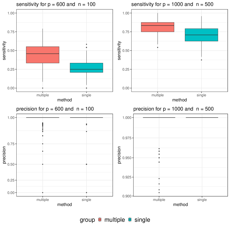
Figure C.1: Sensitivity and precision for the simulation study with $K=2$. Each box shows the distribution of sensitivity or precision among $500$ replicates.

$p$	$n$	$s_{1}^{*}$	$s_{2}^{*}$	sens_mu	sens_si	prec_mu	prec_si
600	100	10	2	0.5976	0.2551	0.9907	0.9328
600	100	10	5	0.495	0.2007	0.9795	0.9269
1000	500	10	2	0.8181	0.7062	0.9936	0.9999
1000	500	10	5	0.7921	0.7025	0.9887	0.9998
1000	500	25	2	0.8261	0.6927	0.9974	0.9999
1000	500	25	5	0.8101	0.6916	0.9938	0.9999

Table C.1: Simulation results for five data sets ($K=5$) with $\sigma=1$. For each setting, the result is averaged over $500$ replicates.

$p$	$n$	$s_{1}^{*}$	$s_{2}^{*}$	$\sigma^{2}$	sens_mu	sens_si	prec_mu	prec_si
600	100	10	2	1	0.4526	0.2632	0.9884	0.9365
600	100	10	5	1	0.3456	0.2045	0.9747	0.9258
600	100	25	2	1	0.1259	0.0656	0.9408	0.7608
600	100	25	5	1	0.089	0.0499	0.8976	0.7229
600	100	10	2	4	0.1233	0.0656	0.7694	0.5547
600	100	10	5	4	0.0931	0.0521	0.7576	0.5482
600	100	25	2	4	0.0499	0.024	0.7389	0.4605
600	100	25	5	4	0.0364	0.0187	0.6643	0.4184
1000	500	10	2	1	0.8121	0.7063	0.9962	1
1000	500	10	5	1	0.7905	0.7011	0.9928	0.9996
1000	500	25	2	1	0.8191	0.696	0.9985	1
1000	500	25	5	1	0.804	0.6949	0.9964	0.9999
1000	500	10	2	4	0.613	0.4655	0.9945	0.9987
1000	500	10	5	4	0.5735	0.4549	0.9901	0.9997
1000	500	25	2	4	0.6077	0.4389	0.9978	0.9999
1000	500	25	5	4	0.577	0.4332	0.9951	0.9997

Table C.2: Simulation results for two data sets ($K=2$). For each setting, the result is averaged over $500$ replicates.

$p$	$n$	$s_{1}^{*}$	$s_{2}^{*}$	$\sigma^{2}$	sens_mu	sens_si	prec_mu	prec_si
600	100	10	2	1	0.5976	0.2551	0.9907	0.9328
600	100	10	5	1	0.495	0.2007	0.9795	0.9269
600	100	25	2	1	0.3344	0.066	0.9877	0.7662
600	100	25	5	1	0.1635	0.0501	0.9655	0.7161
600	100	10	2	4	0.2263	0.0657	0.9408	0.5503
600	100	10	5	4	0.1495	0.0511	0.8889	0.539
600	100	25	2	4	0.0859	0.0241	0.8875	0.4687
600	100	25	5	4	0.0611	0.02037	0.8263	0.4428
1000	500	10	2	1	0.8181	0.7062	0.9936	0.9999
1000	500	10	5	1	0.7921	0.7025	0.9887	0.9998
1000	500	25	2	1	0.8261	0.6927	0.9974	0.9999
1000	500	25	5	1	0.8101	0.6916	0.9938	0.9999
1000	500	10	2	4	0.6641	0.4593	0.992	0.9993
1000	500	10	5	4	0.6167	0.454	0.9865	0.9996
1000	500	25	2	4	0.6776	0.4362	0.9967	0.9998
1000	500	25	5	4	0.6503	0.4301	0.9935	0.9998

Table C.3: Simulation results for five data sets ($K=5$). For each setting, the result is averaged over $500$ replicates.

C.2 Computation Time for muSuSiE and SuSiE

$p$	$n$	$s_{1}^{*}$	$s_{2}^{*}$	$\sigma^{2}$	$K$	time_mu	time_si	$K$	time_mu	time_si
600	100	10	2	1	2	1.75	1.83	5	19.78	4.42
600	100	10	5	1	2	3.09	2.56	5	33.2	6.22
600	100	25	2	1	2	5.18	4.9	5	17.81	12.18
600	100	25	5	1	2	6.46	5.41	5	126.6	13.37
600	100	10	2	4	2	1.43	1.33	5	22.3	3.13
600	100	10	5	4	2	2.33	1.77	5	35.97	4.2
600	100	25	2	4	2	4.33	3.65	5	38.31	8.98
600	100	25	5	4	2	5.34	4.08	5	526.8	10.13
1000	500	10	2	1	2	2.57	2.45	5	15.57	5.73
1000	500	10	5	1	2	3.97	3.28	5	33.23	7.96
1000	500	25	2	1	2	6.79	8.7	5	31.74	21.23
1000	500	25	5	1	2	9.69	10.62	5	284.6	25.94
1000	500	10	2	4	2	2.89	2.63	5	18.41	6.22
1000	500	10	5	4	2	4.79	3.64	5	34.18	9.04
1000	500	25	2	4	2	9.73	10.66	5	38.11	25.92
1000	500	25	5	4	2	13.56	13.25	5	259.2	32.24

Table C.4: Average computation time for muSuSiE and SuSiE measured in seconds. For each setting, the result is averaged over $500$ replicates.

Table C.4 shows the average computation time of the muSuSiE and SuSiE methods for each setting across $500$ replicates. It is evident that the two methods take a similar amount of time when $K=2$. However, as $K$ increases to $5$, the muSuSiE method takes more time than SuSiE. The SuSiE method’s time increases linearly with respect to $K$, while the muSuSiE method’s time increases exponentially.

C.3 Stability Analysis of muSuSiE

prior	$p^{-\omega_{1}}$	$p^{-\omega_{2}}$
prior 1	$p^{-1.1}/2$	$p^{-1.25}$
prior 2	$p^{-1.1}/2$	$p^{-1.5}$
prior 3	$p^{-1.25}$	$p^{-1.5}$
prior 4	$p^{-1.25}$	$p^{-1.75}$
prior 5	$p^{-1.25}$	$p^{-2}$
prior 6	$p^{-1.25}/2$	$p^{-1.5}$

Table C.5: Prior hyperparameters for muSuSiE method with $K=2$ used in Figure C.2.

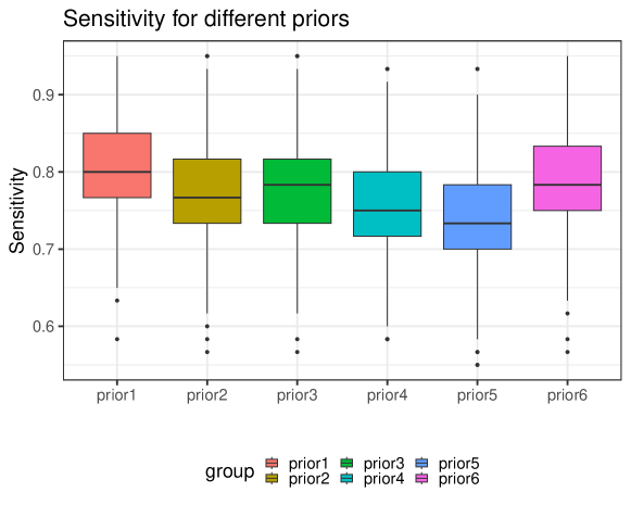
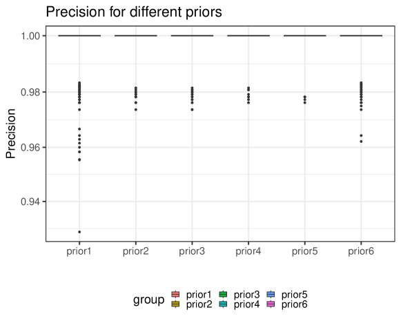
Figure C.2: Simulation results for muSuSiE method with $K=2$, $n=500$, $p=1000$, $\sigma^{2}=1$, $s_{1}^{*}=25$ and $s_{2}^{*}=5$. For each setting, the result is averaged over $500$ replicates.

Consider the setting with $K=2$, $n=500$, $p=1000$, $\sigma^{2}=1$, $s_{1}^{*}=25$, and $s_{2}^{*}=5$. We evaluate the performance of our method with six different priors. Table C.5 enumerates the six priors, and Figure C.2 shows the sensitivity and precision of the different priors across 500 replicates. We observe that the performance of muSuSiE is stable with respect to the choice of prior.

C.4 Simulation Results for Joint MCMC and Separate MCMC

Following Yang et al. (2016); Zhou and Smith (2022), we consider the following posterior distribution for a single-task variable selection problem,

$$\pi(S)\propto p^{-(\kappa_{0}+\kappa_{1})|S|}\frac{1}{(1+g(1-r_{S}^{2}))^{n/2}},$$ (C.1)

where $S\in[p]$ represents the set of activated covariates, $r_{S}^{2}$ refers to the standard R-squared statistic for the model $S$, and $\kappa_{0}$, $\kappa_{1}$ and $g$ are hyperparameters. In this simulation, we set $\kappa_{0}=\kappa_{1}=1$ and $g=p^{2\kappa_{1}}-1$. We run the Metropolis-Hasting (MH) algorithm for each dataset separately in the “separate MCMC” method, only adding and deleting one covariate in each iteration. In each simulation, we run $5\times 10^{4}$ iterations, with the first $10^{4}$ samples for burn-in.

For the “joint MCMC” method, we consider the following joint posterior distribution which is obtained by modifying the prior in (C.1):

$$\pi(\bm{\gamma})\propto\prod_{k=1}^{K}p^{-\omega_{k}a_{k}(\bm{\gamma})}\frac{1}{(1+g(1-r_{S_{k}(\bm{\gamma})}^{2}))^{n/2}}.$$

In each iteration, we propose the next state by uniformly sampling one covariate $j\in[p]$ and a set $I$ from $2^{[K]}\setminus\emptyset$ and then flipping the $j$-th covariate’s activation status in the data sets indexed by $I$. For $K=2$, we set $\omega_{1}=2$ and $\omega_{2}=2.25$. For $K=5$, we use $\omega_{1}=2$, $\omega_{2}=2.25$, $\omega_{3}=2.5$, $\omega_{4}=2.75$, and $\omega_{5}=3$. In each simulation, we run $5\times 10^{4}$ iterations, with the first $10^{4}$ samples for burn-in.

Tables C.6 and C.7 present the results of the two MCMC methods. “sens_sep” and “prec_sep” represent the sensitivity and precision of the separate Metropolis-Hastings (MH) method, respectively; “sens_joint” and “prec_joint” denote the sensitivity and precision of the joint MH method, respectively. We observe that the joint method exhibits greater sensitivity in comparison to the separate method. When the sample size is small, the joint method also has higher precision. This observation aligns with analogous findings from the comparison between muSuSiE and SuSiE. When $K=2$, the joint MCMC approach almost always has lower sensitivity and precision than muSuSiE, except in the setting with $n=500,\sigma^{2}=1$. When $K=5$, the performance of joint MCMC is comparable to that of muSuSiE: joint MCMC tends to have slightly higher sensitivity but lower precision. However, the two MCMC algorithms is considerably more time-consuming than the variational methods, as shown in Table C.8.

$p$	$n$	$s_{1}^{*}$	$s_{2}^{*}$	$\sigma^{2}$	sens_sep	sens_joint	prec_sep	prec_joint
600	100	10	2	1	0.1687	0.3933	0.81	0.9743
600	100	10	5	1	0.1111	0.2619	0.7447	0.9247
600	100	25	2	1	0.024	0.075	0.4258	0.7789
600	100	25	5	1	0.0169	0.0461	0.357	0.6419
600	100	10	2	4	0.0324	0.0718	0.327	0.567
600	100	10	5	4	0.0248	0.0505	0.305	0.5242
600	100	25	2	4	0.0097	0.0228	0.215	0.41
600	100	25	5	4	0.0066	0.0147	0.181	0.3413
1000	500	10	2	1	0.6872	0.8148	1	0.9869
1000	500	10	5	1	0.6765	0.7875	1	0.9738
1000	500	25	2	1	0.6659	0.8304	1	0.9945
1000	500	25	5	1	0.6637	0.8114	1	0.9855
1000	500	10	2	4	0.4148	0.5916	0.995	0.9888
1000	500	10	5	4	0.4001	0.5391	1	0.9752
1000	500	25	2	4	0.359	0.5808	1	0.9958
1000	500	25	5	4	0.3491	0.5567	1	0.9893

Table C.6: Simulation results for standard MCMC method for two data sets ($K=2$). For each setting, the result is averaged over $500$ replicates.

$p$	$n$	$s_{1}^{*}$	$s_{2}^{*}$	$\sigma^{2}$	sens_sep	sens_joint	prec_sep	prec_joint
600	100	10	2	1	0.167	0.6832	0.812	0.9475
600	100	10	5	1	0.1098	0.5613	0.7385	0.9049
600	100	25	2	1	0.0242	0.5713	0.4403	0.9797
600	100	25	5	1	0.018	0.3401	0.3776	0.9657
600	100	10	2	4	0.0324	0.2788	0.3224	0.9441
600	100	10	5	4	0.0246	0.1861	0.3092	0.8979
600	100	25	2	4	0.0091	0.1285	0.214	0.9316
600	100	25	5	4	0.0071	0.0902	0.1888	0.8865
1000	500	10	2	1	0.6847	0.8311	1	0.9237
1000	500	10	5	1	0.6802	0.8016	1	0.8537
1000	500	25	2	1	0.6636	0.8413	1	0.9645
1000	500	25	5	1	0.6599	0.8233	1	0.921
1000	500	10	2	4	0.4102	0.7161	0.9972	0.9403
1000	500	10	5	4	0.3993	0.6565	0.9996	0.8851
1000	500	25	2	4	0.3584	0.7424	0.9996	0.9741
1000	500	25	5	4	0.3476	0.709	1	0.9416

Table C.7: Simulation results for standard MCMC method for five data sets ($K=5$). For each setting, the result is averaged over $500$ replicates.

$p$	$n$	$s_{1}^{*}$	$s_{2}^{*}$	$\sigma^{2}$	$K$	time_joint	time_sep	$K$	time_joint	time_sep
600	100	10	2	1	2	9.4	6.3	5	23.2	8.6
600	100	10	5	1	2	9.3	6.3	5	22.8	8.6
600	100	25	2	1	2	8.9	6.3	5	21.9	8.6
600	100	25	5	1	2	8.8	6.2	5	21.7	8.6
600	100	10	2	4	2	8.7	6.2	5	21.6	8.6
600	100	10	5	4	2	8.7	6.2	5	21.5	8.6
600	100	25	2	4	2	8.7	6.2	5	21.4	8.6
600	100	25	5	4	2	8.6	6.2	5	21.3	8.5
1000	500	10	2	1	2	15.8	10.5	5	39.4	14.3
1000	500	10	5	1	2	17.1	10.5	5	43.2	14.4
1000	500	25	2	1	2	22.9	10.6	5	43.7	14.6
1000	500	25	5	1	2	24.4	10.7	5	20.0	14.7
1000	500	10	2	4	2	13.8	10.4	5	34.2	14.3
1000	500	10	5	4	2	14.5	10.5	5	35.9	14.3
1000	500	25	2	4	2	16.8	10.6	5	42.3	14.5
1000	500	25	5	4	2	17.5	10.6	5	43.5	14.5

Table C.8: Average computation time for separate MCMC and joint MCMC measured in minutes. For each setting, the result is averaged over $500$ replicates.

C.5 Simulation Results for LASSO

Tables C.9 and C.10 show the results obtained using the LASSO method. In comparison with the Bayesian variable selection method, the LASSO method displays higher sensitivity, particularly when the sample size is small ($n=100$). However, the precision of the LASSO method is significantly lower than that of the Bayesian variable selection method. This indicates that the LASSO method tends to select many non-activated covariates.

$p$	$n$	$s_{1}^{*}$	$s_{2}^{*}$	$\sigma^{2}$	sens	prec
600	100	10	2	1	0.6608	0.2227
600	100	10	5	1	0.6443	0.2256
600	100	25	2	1	0.556	0.2597
600	100	25	5	1	0.5274	0.2678
600	100	10	2	4	0.397	0.2661
600	100	10	5	4	0.3817	0.2584
600	100	25	2	4	0.3494	0.285
600	100	25	5	4	0.3262	0.2989
1000	500	10	2	1	0.8683	0.2077
1000	500	10	5	1	0.8733	0.2105
1000	500	25	2	1	0.8859	0.2264
1000	500	25	5	1	0.8825	0.2277
1000	500	10	2	4	0.7414	0.2142
1000	500	10	5	4	0.7433	0.2199
1000	500	25	2	4	0.7687	0.2353
1000	500	25	5	4	0.7678	0.2324

Table C.9: Lasso results for two data sets ($K=2$). For each setting, the result is averaged over $500$ replicates.

$p$	$n$	$s_{1}^{*}$	$s_{2}^{*}$	$\sigma^{2}$	sens	prec
600	100	10	2	1	0.6587	0.2185
600	100	10	5	1	0.6409	0.226
600	100	25	2	1	0.5567	0.2572
600	100	25	5	1	0.5269	0.2689
600	100	10	2	4	0.3931	0.2633
600	100	10	5	4	0.3842	0.2591
600	100	25	2	4	0.3502	0.2833
600	100	25	5	4	0.331	0.2969
1000	500	10	2	1	0.8709	0.2069
1000	500	10	5	1	0.8758	0.2101
1000	500	25	2	1	0.8837	0.2257
1000	500	25	5	1	0.881	0.2281
1000	500	10	2	4	0.741	0.2133
1000	500	10	5	4	0.7474	0.2174
1000	500	25	2	4	0.7654	0.233
1000	500	25	5	4	0.7651	0.2327

Table C.10: Lasso results for five data sets ($K=5$). For each setting, the result is averaged over $500$ replicates.

Appendix D More Simulation Results for Differential DAG Analysis

Recall that we use simulation studies to compare the performance of six methods for joint estimation of multiple DAG models: PC, GES, joint GES, MpenPC, JESC and muSuSiE-DAG. We use $N_{\text{com}}$ to denote the number of shared edges and $N_{\text{pri}}$ to denote the number of edges unique to each data set. In each simulation setting, we report the average number of wrong edges $N_{\text{wrong}}$, the average true positive (TP) rate and the average false positive (FP) rate by ignoring edge directions. In addition, we introduce the fourth measurement metric, the squared Frobenius Norm (F-norm) between the true adjacency matrix and estimated adjacency matrix, which can be calculated as follows. For PC, GES and joint GES method, we let $\hat{\bm{R}}^{(k)}\in\{0,1\}^{p\times p}$ be the estimated adjacency matrix such that $\hat{R}^{(k)}_{ij}=1$ if the edge $(i,j)$ is in the estimated DAG for the $k$-th data set and $\hat{R}^{(k)}_{ij}=0$ otherwise. For muSuSiE-DAG, we let $\hat{\bm{R}}^{(k)}$ be as defined in (19) where each entry is the estimated probability of the edge and thus takes value in $[0,1]$. Let $(\bm{R}^{(k)})_{k=1}^{K}$ be the true adjacency matrices where $R^{(k)}_{ij}=1$ if the edge $(i,j)$ is in the $k$-th true DAG model and $R^{(k)}_{ij}=0$ otherwise. For each method, the F-norm metric is defined as

$$\sum_{i=1}^{p-1}\sum_{j=i+1}^{p}\left(\hat{R}^{(k)}_{ij}+\hat{R}^{(k)}_{ji}-R^{(k)}_{ij}-R^{(k)}_{ji}\right)^{2}.$$

For PC, GES and joint GES, this is equivalent to counting the number of wrong edges. But for muSuSiE-DAG, this statistic in general is different from $N_{\rm{wrong}}$. Table D.4 shows the results for the PC method, Table D.5 for GES and Table D.6 for joint GES. Note that the values of the tuning parameters are also given in the corresponding tables, including the significance level $\alpha$ used in the conditional independent tests for the PC method, and $l_{0}$-penalization parameter $\lambda$ for GES and joint GES. For muSuSiE-DAG, the choice of the parameters $\omega_{1},\dots,\omega_{K}$ is detailed in Table D.1 (for $K=2$) and Table D.2 (for $K=5$). Table D.7 shows the results for our muSuSiEDAG method. Table D.3 compares results for all methods when $K=5$, where for each method we use the optimal tuning parameter.

prior	$p^{-\omega_{1}}$	$p^{-\omega_{2}}$
prior 1	$p^{-1.25}/2$	$p^{-1.5}$
prior 2	$p^{-1.5}/2$	$p^{-2}$
prior 3	$p^{-2}$	$p^{-2.25}$
prior 4	$p^{-2}/2$	$p^{-2.25}$

Table D.1: Prior hyperparameters for muSuSiE-DAG for $K=2$.

prior	$p^{-\omega_{1}}$	$p^{-\omega_{2}}$	$p^{-\omega_{3}}$	$p^{-\omega_{4}}$	$p^{-\omega_{5}}$
prior 1	$p^{-1.5}/5$	$p^{-1.75}/10$	$p^{-2}/10$	$p^{-2.25}/5$	$p^{-2.5}$
prior 2	$p^{-1.75}$	$p^{-2}$	$p^{-2.25}$	$p^{-2.5}$	$p^{-3}$
prior 3	$p^{-1.75}/5$	$p^{-2}/10$	$p^{-2.25}/10$	$p^{-2.5}/5$	$p^{-3}$
prior 4	$p^{-2}$	$p^{-2.25}$	$p^{-2.5}$	$p^{-2.75}$	$p^{-3}$

Table D.2: Prior hyperparameters for muSuSiE-DAG for $K=5$.

As expected, joint methods, joint GES and muSuSiEDAG, have much larger true positive rates and slightly larger false positive rates than the two separate-analysis methods, PC and GES. This is because the joint method can identify edges with low signal strength if it is expressed concurrently in all $K$ data sets, which leads to a higher true positive rate, while the joint method may also identify edges with extremely high signal strength in a single data set as expressed simultaneously in more than one data sets, resulting in a higher false positive rate. Additionally, when the ratio $N_{\text{com}}/N_{\text{pri}}$ is large, implying that the majority of edges are shared, the joint method outperforms the other two by a large margin. When the ratio $N_{\text{com}}/N_{\text{pri}}$ is small, GES may even outperform joint GES. In all cases, our muSuSiE-DAG method has the best performance in terms of the metric $N_{\rm{wrong}}$. We also observe that the results may depend on the choice of the prior parameters (though not significantly), which suggests that in reality one may want to tune the parameters to improve the performance of the algorithm.

method	K	$N_{\text{com}}$	$N_{\text{pri}}$	$N_{\text{wrong}}$	TP	FP
PC	5	100	20	31.844	0.7504	4e-04
GES	5	100	20	23.108	0.8178	3e-04
joint GES	5	100	20	26.828	0.8952	0.0029
MPenPC	5	100	20	194.24	0.8955	0.0372
JESC	5	100	20	33.24	0.9063	0.0045
muSuSiE-DAG	5	100	20	17.064	0.9058	0.0012
PC	5	100	50	43.904	0.7044	3e-04
GES	5	100	50	30.196	0.8157	5e-4
joint GES	5	100	50	36.464	0.8794	0.0038
MPenPC	5	100	50	153.788	0.8654	0.0275
JESC	5	100	50	34.996	0.9118	0.0045
muSuSiE-DAG	5	100	50	28.572	0.8755	0.002
PC	5	50	50	25.116	0.7309	1e-04
GES	5	50	50	19.288	0.8166	2e-04
joint GES	5	50	50	32.836	0.8492	0.0036
MPenPC	5	50	50	224.876	0.9098	0.0441
JESC	5	50	50	31.496	0.909	0.0046
muSuSiE-DAG	5	50	50	18.58	0.8529	8e-04

Table D.3: Simulation results for joint estimation of multiple DAG models with $K=5$.

$K$	$\alpha$	$N_{\text{com}}$	$N_{\text{pri}}$	$N_{\text{wrong}}$	TP	FP	F-norm
2	1e-04	100	20	38.52	0.68	0	38.52
2	5e-04	100	20	34.1	0.7183	1e-04	34.1
2	0.001	100	20	32.04	0.7373	1e-04	32.04
2	0.005	100	20	28.29	0.7822	4e-04	28.29
2	0.01	100	20	28.55	0.8009	0.001	28.55
2	0.05	100	20	45.83	0.8523	0.0058	45.83
2	1e-04	100	50	54.04	0.6404	0	54.04
2	5e-04	100	50	47.93	0.6823	1e-04	47.93
2	0.001	100	50	45.32	0.7007	1e-04	45.32
2	0.005	100	50	39.37	0.7475	3e-04	39.37
2	0.01	100	50	37.93	0.7674	6e-04	37.93
2	0.05	100	50	44.9	0.8225	0.0038	44.9
2	1e-04	50	50	28.13	0.7192	0	28.13
2	5e-04	50	50	24.59	0.7572	1e-04	24.59
2	0.001	50	50	23.44	0.7723	1e-04	23.44
2	0.005	50	50	21.9	0.8121	6e-04	21.9
2	0.01	50	50	23.34	0.8312	0.0013	23.34
2	0.05	50	50	47.78	0.8796	0.0073	47.78
5	1e-04	100	20	43.108	0.6413	0	43.108
5	5e-04	100	20	38.428	0.6816	0	38.428
5	0.001	100	20	36.264	0.701	1e-04	36.264
5	0.005	100	20	32.044	0.7504	4e-04	32.044
5	0.01	100	20	31.844	0.7725	9e-04	31.844
5	0.05	100	20	47.924	0.8286	0.0056	47.924
5	1e-04	100	50	62.304	0.5854	0	62.304
5	5e-04	100	50	55.508	0.6313	0	55.508
5	0.001	100	50	52.528	0.6521	1e-04	52.528
5	0.005	100	50	45.78	0.7044	3e-04	45.78
5	0.01	100	50	43.904	0.7276	6e-04	43.904
5	0.05	100	50	50.608	0.7897	0.0039	50.608
5	1e-04	50	50	33	0.6703	0	33
5	5e-04	50	50	29.064	0.7114	0	29.064
5	0.001	50	50	27.424	0.7309	1e-04	27.424
5	0.005	50	50	25.116	0.779	6e-04	25.116
5	0.01	50	50	26.036	0.8002	0.0012	26.036
5	0.05	50	50	49.848	0.8535	0.0072	49.848

Table D.4: Simulation results for the PC algorithm. $N_{\rm{wrong}}$ is the same as F-norm by definition.

$K$	$\lambda$	$N_{\text{com}}$	$N_{\text{pri}}$	$N_{\text{wrong}}$	TP	FP	F-norm
2	1	100	20	32.47	0.9152	0.0046	32.47
2	2	100	20	19.67	0.8482	3e-04	19.67
2	3	100	20	26.76	0.7837	2e-04	26.76
2	4	100	20	33.26	0.7269	1e-04	33.26
2	5	100	20	39.03	0.6777	1e-04	39.03
2	1	100	50	35.26	0.9191	0.0048	35.26
2	2	100	50	24.84	0.8505	5e-04	24.84
2	3	100	50	33.12	0.7895	3e-04	33.12
2	4	100	50	40.31	0.7383	2e-04	40.31
2	5	100	50	47.35	0.6893	2e-04	47.35
2	1	50	50	29	0.9223	0.0043	29
2	2	50	50	15.74	0.8514	2e-04	15.74
2	3	50	50	21.15	0.7925	1e-04	21.15
2	4	50	50	26.47	0.7374	0	26.47
2	5	50	50	31.16	0.6904	0	31.16
5	1	100	20	35.548	0.8955	0.0047	35.548
5	2	100	20	23.108	0.8178	3e-04	23.108
5	3	100	20	31.008	0.7466	1e-04	31.008
5	4	100	20	38.44	0.6824	1e-04	38.44
5	5	100	20	46.012	0.6184	0	46.012
5	1	100	50	40.36	0.8953	0.0051	40.36
5	2	100	50	30.196	0.8157	5e-04	30.196
5	3	100	50	39.664	0.744	3e-04	39.664
5	4	100	50	48.988	0.6791	2e-04	48.988
5	5	100	50	58.332	0.615	1e-04	58.332
5	1	50	50	32.58	0.8976	0.0046	32.58
5	2	50	50	19.288	0.8166	2e-04	19.288
5	3	50	50	25.852	0.7453	1e-04	25.852
5	4	50	50	32.2	0.68	0	32.2
5	5	50	50	38.18	0.6195	0	38.18

Table D.5: Simulation results for the GES method. $N_{\rm{wrong}}$ is the same as F-norm by definition.

$K$	$\lambda$	$N_{\text{com}}$	$N_{\text{pri}}$	$N_{\text{wrong}}$	TP	FP	F-norm
2	1	100	20	38.84	0.9172	0.0059	38.84
2	2	100	20	15.4	0.9126	0.001	15.4
2	3	100	20	16.48	0.8957	8e-04	16.48
2	4	100	20	18.62	0.875	7e-04	18.62
2	5	100	20	20.93	0.8531	7e-04	20.93
2	1	100	50	46.5	0.9179	0.007	46.5
2	2	100	50	24.7	0.9003	0.002	24.7
2	3	100	50	25.72	0.879	0.0016	25.72
2	4	100	50	28.65	0.8554	0.0014	28.65
2	5	100	50	31.98	0.8295	0.0013	31.98
2	1	50	50	38.28	0.9042	0.0059	38.28
2	2	50	50	22.91	0.883	0.0023	22.91
2	3	50	50	24.68	0.8536	0.002	24.68
2	4	50	50	27.78	0.8186	0.002	27.78
2	5	50	50	30.53	0.788	0.0019	30.53
5	1	100	20	74.608	0.8935	0.0127	74.608
5	2	100	20	26.828	0.8952	0.0029	26.828
5	3	100	20	23.332	0.8877	0.002	23.332
5	4	100	20	24.196	0.8773	0.0019	24.196
5	5	100	20	24.728	0.8698	0.0019	24.728
5	1	100	50	90.516	0.8964	0.0155	90.516
5	2	100	50	36.464	0.8794	0.0038	36.464
5	3	100	50	35.704	0.8591	0.003	35.704
5	4	100	50	38.364	0.8399	0.003	38.364
5	5	100	50	40.32	0.8222	0.0028	40.32
5	1	50	50	70.392	0.8726	0.0118	70.392
5	2	50	50	32.836	0.8492	0.0036	32.836
5	3	50	50	33.716	0.8198	0.0032	33.716
5	4	50	50	36.356	0.7922	0.0032	36.356
5	5	50	50	39.744	0.7621	0.0033	39.744

Table D.6: Simulation results for the joint GES method. $N_{\rm{wrong}}$ is the same as F-norm by definition.

$K$	prior	$N_{\text{com}}$	$N_{\text{pri}}$	$N_{\text{wrong}}$	TP	FP	F-norm
2	prior 1	100	20	18.63	0.9248	0.002	16.6747
2	prior 2	100	20	14.77	0.9052	7e-04	12.6597
2	prior 3	100	20	13.03	0.9081	4e-04	10.9038
2	prior 4	100	20	12.91	0.9138	5e-04	11.1051
2	prior 1	100	50	27.17	0.9103	0.0028	24.693
2	prior 2	100	50	19.84	0.8983	9e-04	17.2605
2	prior 3	100	50	19.56	0.8933	7e-04	17.0741
2	prior 4	100	50	18.45	0.9003	7e-04	16.45
2	prior 1	50	50	17.84	0.8995	0.0016	16.547
2	prior 2	50	50	15.03	0.8819	7e-04	13.2731
2	prior 3	50	50	15.4	0.8727	5e-04	13.6451
2	prior 4	50	50	15.03	0.8762	5e-04	13.4162
5	prior 1	100	20	19.684	0.9243	0.0022	16.9472
5	prior 2	100	20	26.64	0.8808	0.0025	23.518
5	prior 3	100	20	17.064	0.9058	0.0012	14.2844
5	prior 4	100	20	20.636	0.8955	0.0017	17.7576
5	prior 1	100	50	30.74	0.8913	0.003	27.2652
5	prior 2	100	50	43.292	0.8515	0.0043	39.0037
5	prior 3	100	50	28.572	0.8755	0.002	25.0959
5	prior 4	100	50	32.144	0.8679	0.0025	28.5295
5	prior 1	50	50	19.684	0.8681	0.0013	17.643
5	prior 2	50	50	25.832	0.8418	0.002	23.5776
5	prior 3	50	50	18.58	0.8529	8e-04	16.5723
5	prior 4	50	50	21.304	0.85	0.0013	19.215

Table D.7: Simulation results for the muSuSiE-DAG method.

$N_{\text{com}}$	$N_{\text{pri}}$	Joint GES	muSuSiE-DAG
50	50	0.3268	4.1788
100	50	0.4663	5.0471
100	20	0.3173	4.3901

Table D.8: Average computation time for the joint GES and muSuSiE-DAG method for $K=2$ measured in hours.

D.1 Convergence of MCMC

The structure learning is by nature computationally very expensive. In order to demonstrate the convergence of our MCMC algorithm, we simulate one instance of $(\mathcal{G}^{(k)})_{k=1}K$ and $(\bm{X}^{(k)})_{k=1}^{K}$ with $K=2$, $n_{\text{com}}=50$, and $n_{\text{pri}}=50$. We run the algorithm 50 times (for the same data set), each with a maximum of $10^{6}$ iterations. The log-likelihood with respect to the number of iterations is depicted in Figure D.1. It can be observed that the algorithm converges after approximately $6\times 10^{5}$ iterations, which is relatively large. The simulation study presented in Section 5 uses a total of $10^{5}$ MCMC iterations, which appears to be sufficient for yielding satisfactory results.

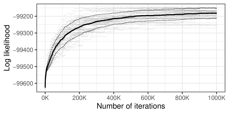
Figure D.1: Log-likelihood trace plot for muSuSiE-DAG under the setting with $K=2$, $n_{\text{com}}=50$ and $n_{\text{pri}}=50$. Trajectories of all 50 runs are shown individually in gray. The solid line denotes the average over 50 runs, and dashed lines indicate one standard derivation above and below the average.

Appendix E Additional Results for Real Data Analysis

Table E.1 shows additional results for the real data example presented in Section 6 with other choices of the tuning parameters. Results for PC, GES and joint GES methods combined with stability selection (Meinshausen and Bühlmann, 2010), which we implement using stabsel function in the stabs package, are shown in Table E.2. There is a hyperparameter cutoff in stabsel function, which we denote by “cutoff1” in the table. The stabsel function returns a selection probability for each edge, and as a result, we need to choose a threshold, denoted by “cutoff2”, to obtain a DAG from the stable selection result. In Table E.2, we list the results for $\text{cutoff1}=0.6,0.7,0.8,0.9$ and $\text{cutoff2}=0.55,0.75$.

Method	Parameters	$|\mathcal{G}_{1}|$	$|\mathcal{G}_{2}|$	$|\mathcal{G}_{1}\cap\mathcal{G}_{2}|$	$N_{\text{total}}$	ratio
PC	$\alpha=1e-04$	12	26	7	31	0.2258
PC	$\alpha=5e-04$	19	38	13	44	0.2955
PC	$\alpha=0.001$	23	39	14	48	0.2917
PC	$\alpha=0.005$	33	60	18	75	0.24
PC	$\alpha=0.01$	42	69	19	92	0.2065
PC	$\alpha=0.05$	73	109	24	158	0.1519
GES	$\lambda=1$	150	238	49	339	0.1445
GES	$\lambda=2$	99	148	43	204	0.2108
GES	$\lambda=3$	78	108	34	152	0.2237
GES	$\lambda=4$	75	92	32	135	0.237
GES	$\lambda=5$	75	87	31	131	0.2366
joint GES	$\lambda=1$	77	85	68	94	0.7234
joint GES	$\lambda=2$	78	78	72	84	0.8571
joint GES	$\lambda=3$	76	76	72	80	0.9
joint GES	$\lambda=4$	76	76	73	79	0.9241
joint GES	$\lambda=5$	76	75	73	78	0.9359
muSuSiE-DAG	$p^{-\omega_{1}}=p^{-1.25},\,p^{-\omega_{2}}=p^{-2}$	33	115	30	118	0.2542
muSuSiE-DAG	$p^{-\omega_{1}}=p^{-1.5},\,p^{-\omega_{2}}=p^{-2.5}$	27	95	25	97	0.2577
muSuSiE-DAG	$p^{-\omega_{1}}=p^{-1.5}/2,\,p^{-\omega_{2}}=p^{-2}$	43	93	42	94	0.4468
muSuSiE-DAG	$p^{-\omega_{1}}=p^{-2},\,p^{-\omega_{2}}=p^{-3.5}$	17	68	14	71	0.1972
muSuSiE-DAG	$p^{-\omega_{1}}=p^{-2}/2,\,p^{-\omega_{2}}=p^{-3.5}$	20	67	19	68	0.2794
muSuSiE-DAG	$p^{-\omega_{1}}=p^{-\omega_{2}}=p^{-2}$	57	83	57	83	0.6867

Table E.1: More results for the real data analysis. $|\mathcal{G}_{k}|$: number of edges in the estimated DAG for the $k$-th group; $|\mathcal{G}_{1}\cap\mathcal{G}_{2}|$: number of edges shared by both DAGs; $N_{\text{total}}$: total number of edges in two DAGs; ratio: the ratio of $|\mathcal{G}_{1}\cap\mathcal{G}_{2}|$ to $N_{\text{total}}$.

Method	cutoff1	cutoff2	$|\mathcal{G}_{1}|$	$|\mathcal{G}_{2}|$	$|\mathcal{G}_{1}\cap\mathcal{G}_{2}|$	$N_{\text{total}}$	ratio
PC	0.6	0.55	49	85	19	115	0.1652
PC	0.6	0.75	36	63	18	81	0.2222
PC	0.7	0.55	48	85	19	114	0.1667
PC	0.7	0.75	37	63	19	81	0.2346
PC	0.8	0.55	51	87	20	118	0.1695
PC	0.8	0.75	35	65	18	82	0.2195
PC	0.9	0.55	50	87	20	117	0.1709
PC	0.9	0.75	36	62	18	80	0.225
GES	0.6	0.55	99	150	41	208	0.1971
GES	0.6	0.75	65	97	32	130	0.2462
GES	0.7	0.55	96	152	41	207	0.1981
GES	0.7	0.75	68	100	34	134	0.2537
GES	0.8	0.55	99	149	39	209	0.1866
GES	0.8	0.75	69	94	32	131	0.2443
GES	0.9	0.55	98	155	45	208	0.2163
GES	0.9	0.75	68	97	33	132	0.25
joint GES	0.6	0.55	60	61	57	64	0.8906
joint GES	0.6	0.75	57	58	55	60	0.9167
joint GES	0.7	0.55	67	70	63	74	0.8514
joint GES	0.7	0.75	58	58	57	59	0.9661
joint GES	0.8	0.55	65	71	56	80	0.7
joint GES	0.8	0.75	53	56	51	58	0.8793
joint GES	0.9	0.55	65	72	60	77	0.7792
joint GES	0.9	0.75	53	56	53	56	0.9464

Table E.2: More results for PC, GES and joint GES methods in the real data analysis. $|\mathcal{G}_{k}|$: number of edges in the estimated DAG for the $k$-th group; $|\mathcal{G}_{1}\cap\mathcal{G}_{2}|$: number of edges shared by both DAGs; $N_{\text{total}}$: total number of edges in two DAGs; ratio: the ratio of $|\mathcal{G}_{1}\cap\mathcal{G}_{2}|$ to $N_{\text{total}}$.

References

- Agrawal et al. (2018) Raj Agrawal, Caroline Uhler, and Tamara Broderick. Minimal I-MAP MCMC for scalable structure discovery in causal DAG models. In International Conference on Machine Learning, pages 89–98, 2018.
- Blei et al. (2017) David M Blei, Alp Kucukelbir, and Jon D McAuliffe. Variational inference: A review for statisticians. Journal of the American Statistical Association, 112(518):859–877, 2017.
- Bonilla et al. (2007) Edwin V Bonilla, Kian Chai, and Christopher Williams. Multi-task Gaussian process prediction. Advances in Neural Information Processing Systems, 20, 2007.
- Carbonetto and Stephens (2012) Peter Carbonetto and Matthew Stephens. Scalable variational inference for Bayesian variable selection in regression, and its accuracy in genetic association studies. Bayesian Analysis, 7(1):73–108, 2012.
- Castelletti et al. (2020) Federico Castelletti, Luca La Rocca, Stefano Peluso, Francesco C Stingo, and Guido Consonni. Bayesian learning of multiple directed networks from observational data. Statistics in Medicine, 39(30):4745–4766, 2020.
- Chen et al. (2021) Xinshi Chen, Haoran Sun, Caleb Ellington, Eric Xing, and Le Song. Multi-task learning of order-consistent causal graphs. Advances in Neural Information Processing Systems, 34, 2021.
- Chickering (2002) David Maxwell Chickering. Optimal structure identification with greedy search. Journal of Machine Learning Research, 3(Nov):507–554, 2002.
- Danaher et al. (2014) Patrick Danaher, Pei Wang, and Daniela M Witten. The joint graphical lasso for inverse covariance estimation across multiple classes. Journal of the Royal Statistical Society: Series B (Statistical Methodology), 76(2):373–397, 2014.
- Ellis and Wong (2008) Byron Ellis and Wing Hung Wong. Learning causal Bayesian network structures from experimental data. Journal of the American Statistical Association, 103(482):778–789, 2008.
- Fiers et al. (2018) Mark WEJ Fiers, Liesbeth Minnoye, Sara Aibar, Carmen Bravo González-Blas, Zeynep Kalender Atak, and Stein Aerts. Mapping gene regulatory networks from single-cell omics data. Briefings in functional genomics, 17(4):246–254, 2018.
- Fronk and Giudici (2004) Eva-Maria Fronk and Paolo Giudici. Markov Chain Monte Carlo model selection for DAG models. Statistical Methods and Applications, 13(3):259–273, 2004.
- George and McCulloch (1993) Edward I George and Robert E McCulloch. Variable selection via Gibbs sampling. Journal of the American Statistical Association, 88(423):881–889, 1993.
- Ghoshal et al. (2019) Asish Ghoshal, Kevin Bello, and Jean Honorio. Direct learning with guarantees of the difference DAG between structural equation models. arXiv preprint arXiv:1906.12024, 2019.
- Gonçalves et al. (2016) André R Gonçalves, Fernando J Von Zuben, and Arindam Banerjee. Multi-task sparse structure learning with gaussian copula models. The Journal of Machine Learning Research, 17(1):1205–1234, 2016.
- Guo et al. (2011) Shengbo Guo, Onno Zoeter, and Cédric Archambeau. Sparse Bayesian multi-task learning. Advances in Neural Information Processing Systems, 24, 2011.
- Harris and Drton (2013) Naftali Harris and Mathias Drton. PC algorithm for nonparanormal graphical models. Journal of Machine Learning Research, 14(11), 2013.
- Hernández-Lobato et al. (2015) Daniel Hernández-Lobato, José Miguel Hernández-Lobato, and Zoubin Ghahramani. A probabilistic model for dirty multi-task feature selection. In International Conference on Machine Learning, pages 1073–1082. PMLR, 2015.
- Huang et al. (2016) Xichen Huang, Jin Wang, and Feng Liang. A variational algorithm for Bayesian variable selection. arXiv preprint arXiv:1602.07640, 2016.
- Ishwaran and Rao (2005) Hemant Ishwaran and J Sunil Rao. Spike and slab variable selection: Frequentist and Bayesian strategies. The Annals of Statistics, 33(2):730–773, 2005.
- Jalali et al. (2010) Ali Jalali, Sujay Sanghavi, Chao Ruan, and Pradeep Ravikumar. A dirty model for multi-task learning. Advances in Neural Information Processing Systems, 23, 2010.
- Jeong and Ghosal (2021) Seonghyun Jeong and Subhashis Ghosal. Unified bayesian theory of sparse linear regression with nuisance parameters. Electronic Journal of Statistics, 15(1):3040–3111, 2021.
- Jiang and Tanner (2008) Wenxin Jiang and Martin A Tanner. Gibbs posterior for variable selection in high-dimensional classification and data mining. The Annals of Statistics, 36(5):2207–2231, 2008.
- Johnson and Rossell (2012) Valen E Johnson and David Rossell. Bayesian model selection in high-dimensional settings. Journal of the American Statistical Association, 107(498):649–660, 2012.
- Kalisch et al. (2012) Markus Kalisch, Martin Mächler, Diego Colombo, Marloes H Maathuis, and Peter Bühlmann. Causal inference using graphical models with the R package pcalg. Journal of Statistical Software, 47:1–26, 2012.
- Kanehisa et al. (2012) Minoru Kanehisa, Susumu Goto, Yoko Sato, Miho Furumichi, and Mao Tanabe. KEGG for integration and interpretation of large-scale molecular data sets. Nucleic Acids Research, 40(D1):D109–D114, 2012.
- Koller and Friedman (2009) Daphne Koller and Nir Friedman. Probabilistic graphical models: Principles and techniques. MIT press, 2009.
- Kuipers and Moffa (2017) Jack Kuipers and Giusi Moffa. Partition MCMC for inference on acyclic digraphs. Journal of the American Statistical Association, 112(517):282–299, 2017.
- Kuipers et al. (2022) Jack Kuipers, Polina Suter, and Giusi Moffa. Efficient sampling and structure learning of Bayesian networks. Journal of Computational and Graphical Statistics, pages 1–12, 2022.
- Lee and Cao (2022) Kyoungjae Lee and Xuan Cao. Bayesian joint inference for multiple directed acyclic graphs. Journal of Multivariate Analysis, 191:105003, 2022.
- Li et al. (2020) Yan Li, Dayou Liu, Tengfei Li, and Yungang Zhu. Bayesian differential analysis of gene regulatory networks exploiting genetic perturbations. BMC Bioinformatics, 21(1):1–13, 2020.
- Liu et al. (2019) Jianyu Liu, Wei Sun, and Yufeng Liu. Joint skeleton estimation of multiple directed acyclic graphs for heterogeneous population. Biometrics, 75(1):36–47, 2019.
- Lounici et al. (2009) Karim Lounici, Massimiliano Pontil, Alexandre B Tsybakov, and Sara Van De Geer. Taking advantage of sparsity in multi-task learning. arXiv preprint arXiv:0903.1468, 2009.
- Lounici et al. (2011) Karim Lounici, Massimiliano Pontil, Sara Van De Geer, and Alexandre B Tsybakov. Oracle inequalities and optimal inference under group sparsity. The Annals of Statistics, 39(4):2164–2204, 2011.
- Meinshausen and Bühlmann (2010) Nicolai Meinshausen and Peter Bühlmann. Stability selection. Journal of the Royal Statistical Society: Series B (Statistical Methodology), 72(4):417–473, 2010.
- Nandy et al. (2018) Preetam Nandy, Alain Hauser, and Marloes H Maathuis. High-dimensional consistency in score-based and hybrid structure learning. The Annals of Statistics, 46(6A):3151–3183, 2018.
- Narisetty and He (2014) Naveen Naidu Narisetty and Xuming He. Bayesian variable selection with shrinking and diffusing priors. The Annals of Statistics, 42(2):789–817, 2014.
- Niu et al. (2018) Xiangyu Niu, Yifan Sun, and Jinyuan Sun. Latent group structured multi-task learning. In 2018 52nd Asilomar Conference on Signals, Systems, and Computers, pages 850–854. IEEE, 2018.
- Ormerod et al. (2017) John T Ormerod, Chong You, and Samuel Müller. A variational Bayes approach to variable selection. Electronic Journal of Statistics, 11:3549–3594, 2017.
- Oyen and Lane (2012) Diane Oyen and Terran Lane. Leveraging domain knowledge in multitask Bayesian network structure learning. In Twenty-Sixth AAAI Conference on Artificial Intelligence, 2012.
- Peterson et al. (2015) Christine Peterson, Francesco C Stingo, and Marina Vannucci. Bayesian inference of multiple Gaussian graphical models. Journal of the American Statistical Association, 110(509):159–174, 2015.
- Peterson and Stingo (2021) Christine B Peterson and Francesco C Stingo. Bayesian estimation of single and multiple graphs. In Handbook of Bayesian Variable Selection, pages 327–348. Chapman and Hall/CRC, 2021.
- Peterson et al. (2020) Christine B Peterson, Nathan Osborne, Francesco C Stingo, Pierrick Bourgeat, James D Doecke, and Marina Vannucci. Bayesian modeling of multiple structural connectivity networks during the progression of Alzheimer’s disease. Biometrics, 76(4):1120–1132, 2020.
- Ray and Szabó (2021) Kolyan Ray and Botond Szabó. Variational Bayes for high-dimensional linear regression with sparse priors. Journal of the American Statistical Association, pages 1–12, 2021.
- Ray and Szabó (2022) Kolyan Ray and Botond Szabó. Variational Bayes for high-dimensional linear regression with sparse priors. Journal of the American Statistical Association, 117(539):1270–1281, 2022.
- Shaddox et al. (2020) Elin Shaddox, Christine B Peterson, Francesco C Stingo, Nicola A Hanania, Charmion Cruickshank-Quinn, Katerina Kechris, Russell Bowler, and Marina Vannucci. Bayesian inference of networks across multiple sample groups and data types. Biostatistics, 21(3):561–576, 2020.
- Spirtes et al. (2000) Peter Spirtes, Clark N Glymour, Richard Scheines, and David Heckerman. Causation, prediction, and search. MIT press, 2000.
- Tothill et al. (2008) Richard W Tothill, Anna V Tinker, Joshy George, Robert Brown, Stephen B Fox, Stephen Lade, Daryl S Johnson, Melanie K Trivett, Dariush Etemadmoghadam, Bianca Locandro, et al. Novel molecular subtypes of serous and endometrioid ovarian cancer linked to clinical outcome. Clinical cancer research, 14(16):5198–5208, 2008.
- Van de Sande et al. (2020) Bram Van de Sande, Christopher Flerin, Kristofer Davie, Maxime De Waegeneer, Gert Hulselmans, Sara Aibar, Ruth Seurinck, Wouter Saelens, Robrecht Cannoodt, Quentin Rouchon, Toni Verbeiren, Dries De Maeyer, Joke Reumers, Yvan Saeys, and Stein Aerts. A scalable SCENIC workflow for single-cell gene regulatory network analysis. Nature Protocols, 15(7):2247–2276, 2020.
- Wang et al. (2020a) Gao Wang, Abhishek Sarkar, Peter Carbonetto, and Matthew Stephens. A simple new approach to variable selection in regression, with application to genetic fine mapping. Journal of the Royal Statistical Society: Series B (Statistical Methodology), 82(5):1273–1300, 2020a.
- Wang et al. (2020b) Yuhao Wang, Santiago Segarra, and Caroline Uhler. High-dimensional joint estimation of multiple directed Gaussian graphical models. Electronic Journal of Statistics, 14(1):2439–2483, 2020b.
- Yajima et al. (2015) Masanao Yajima, Donatello Telesca, Yuan Ji, and Peter Müller. Detecting differential patterns of interaction in molecular pathways. Biostatistics, 16(2):240–251, 2015.
- Yang et al. (2016) Yun Yang, Martin J Wainwright, and Michael I Jordan. On the computational complexity of high-dimensional Bayesian variable selection. The Annals of Statistics, 44(6):2497–2532, 2016.
- Zhang et al. (2020) Aiying Zhang, Gemeng Zhang, Vince D Calhoun, and Yu-Ping Wang. Causal brain network in schizophrenia by a two-step bayesian network analysis. In Medical Imaging 2020: Imaging Informatics for Healthcare, Research, and Applications, volume 11318, pages 316–321. SPIE, 2020.
- Zhang and Yang (2021) Yu Zhang and Qiang Yang. A survey on multi-task learning. IEEE Transactions on Knowledge and Data Engineering, 2021.
- Zhou and Smith (2022) Quan Zhou and Aaron Smith. Rapid convergence of informed importance tempering. In International Conference on Artificial Intelligence and Statistics, pages 10939–10965. PMLR, 2022.