Optimal Estimation of Generic Dynamics by Path-Dependent Neural Jump ODEs

Abstract

This paper studies the problem of forecasting general stochastic processes using a path-dependent extension of the Neural Jump ODE (NJ-ODE) framework (Herrera et al., 2021). While NJ-ODE was the first framework to establish convergence guarantees for the prediction of irregularly observed time series, these results were limited to data stemming from Itô-diffusions with complete observations, in particular Markov processes, where all coordinates are observed simultaneously. In this work, we generalise these results to generic, possibly non-Markovian or discontinuous, stochastic processes with incomplete observations, by utilising the reconstruction properties of the signature transform. These theoretical results are supported by empirical studies, where it is shown that the path-dependent NJ-ODE outperforms the original NJ-ODE framework in the case of non-Markovian data. Moreover, we show that PD-NJ-ODE can be applied successfully to classical stochastic filtering problems and to limit order book (LOB) data.

1 Introduction

The processing and prediction of time series data is of great importance in many data-driven fields such as economics, finance, and medicine. In recent years a lot of progress was made improving the machine learning techniques and, in particular, the neural network based ones, to be able to deal with more complicated problem settings. Recurrent Neural networks (RNNs) constituted the starting point to deal with discrete time series of variable and possibly unbounded length. Their main constraint is the underlying assumption that observations occur in regular time steps. A first step in the direction of irregular observation times was made by defining the RNN’s latent variable continuously in time with some time-decay (e.g. exponential) directed to $0$ (Che et al., 2018; Cao et al., 2018). However, since this is a rather stiff framework, neural ODEs (Chen et al., 2018) set a new milestone by making the continuously-in-time defined latent dynamics trainable through a neural network. Finally, combining this trainable continuous-in-time latent framework with an RNN cell, led to a framework for irregularly sampled time series data (Rubanova et al., 2019; Brouwer et al., 2019).

In machine learning applications to time series data, we distinguish between two different problem settings. Firstly, the labelling problem, where the entire time series is processed with the goal to determine a class or value describing some feature of this time series. An example would be a time series consisting of health parameters of a hospital patient with the aim of predicting whether the patient will develop a certain disease within the next days. And secondly, the forecasting problem where the goal is to process the known past values of the time series to predict how it will develop in the future. If this is done such that the entire time series of a predefined length is processed and certain time points in the future are predicted, then this can be viewed as a special case of the labelling problem (with a possibly infinite dimensional output). Here, we will refer to this as offline forecasting. On the other hand, if the goal is to forecast continuously in time, where for every time point a prediction can be made depending only on the past observations, this is a different problem, which we refer to as online forecasting. Here, the algorithm has to dynamically predict based on the known past observations as long as no new information is available and then processes new observations (and adjust itself accordingly), whenever they become available. Coming back to our previous example, this would mean to continuously in time forecast how the health parameters will evolve, given those observations which were made up to the current time. In this work, which is the second part and generalisation of the Neural Jump ODE (NJ-ODE) framework (Herrera et al., 2021), we consider precisely this problem. In particular, our goal is to make optimal forecasts, where optimality in this work is meant in terms of the $L^{2}$-norm.

While NJ-ODE was the first framework in which theoretical convergence guarantees of the model output to the optimal prediction were derived, relatively restrictive assumptions on the underlying dynamics of the time series data were needed. In particular, the data has to stem from an Itô diffusion with several constraints on its drift and diffusion. This implies that paths of the dataset are continuous and Markovian (no path-dependence). Moreover, it is necessary that observations are complete, i.e., that all coordinates are observed simultaneously at each observation time. In the present work, we extend the NJ-ODE such that it can be applied to a very general set of stochastic processes that satisfy only weak regularity conditions. Since some of these constraints might seem a bit abstract at first, we provide several examples for which we prove that the assumptions are satisfied. Some examples are processes with jumps, fractional Brownian motion (rough paths with path-dependence) and multidimensional correlated processes with incomplete observations. Moreover, we show how the NJ-ODE framework can be used to perform not only prediction but also uncertainty estimation and how it can be applied to the stochastic filtering problem. Our theoretical results are based on the universal approximation property of neural networks and the signature transform.

1.1 Related Work

Recurrent neural networks (Rumelhart et al., 1985; Jordan, 1997) and the neural ODE (Chen et al., 2018) are the two main ingredients for the (path-dependent) NJ-ODE model. The first works in which they were combined to a model similar to the one we use were Rubanova et al. (2019); Brouwer et al. (2019). In contrast to our framework, the latent ODE (Rubanova et al., 2019) is a model for the offline forecasting problem, where an encoder-decoder type model is used. First, the ODE-RNN encoder processes the entire time series of observations to generate an initial latent variable, which is then used as starting point for a neural ODE that produces the forecasts. In comparison to that, GRU-ODE-Bayes (Brouwer et al., 2019) uses the same model framework as we do for online forecasting. The main difference to NJ-ODE lies in the objective function and training framework. In particular, no convergence guarantees exist for GRU-ODE-Bayes, as was discussed in detail in Herrera et al. (2021).

Being the predecessor, NJ-ODE (Herrera et al., 2021) clearly is the most related work to the present one. While the main structure of the model and of the theoretical results is the same, we make many important changes to extend the theory from a class of Itô processes to a large class of generic stochastic processes. A major ingredient to do this is the signature transform (Chevyrev & Kormilitzin, 2016; Kiraly & Oberhauser, 2019; Fermanian, 2020), which allows us to approximate path dependent behaviours.

The most related work in the context of the labelling problem, besides Rubanova et al. (2019), is the neural controlled differential equation (NCDE) (Kidger et al., 2020). Similar to neural ODEs, it integrates a neural network, however, not against time but against the linear or spline interpolation of the observed time series. The NCDE can only be used for the labelling problem (including offline forecasting), but not for the online forecasting problem, since its interpolation of the observations depends on future data (cf. Morrill et al. (2022)). Hence, in general its output at an intermediate time $t$ is not measurable with respect to the information available at this time. In Morrill et al. (2022), the NCDE was extended by using the rectilinear (instead of linear or spline) interpolation of the data to circumvent this problem and make it applicable to online forecasting tasks. Nevertheless, the authors did not apply it to the type of online prediction tasks we are most interested in, where the value of a stochastic process should be predicted based on previous discrete observations of this process, but only to labelling problems (making the comment that these labelling problems can now be addressed in an online manner). In line with this, no convergence guarantees are provided for such problems.

Neural rough differential equations (NRDE) (Morrill et al., 2021) are yet another extension of NCDEs, where a neural network is piece-wisely integrated on intervals against time and multiplied with the depth-$N$ log-signature transform computed over the respective interval. The advantage of this method over NCDEs is that the intervals can be chosen larger than the intervals between consecutive observation times, since the log-signature can compress the path information on the entire interval. In particular, no information is lost, while this is the case when increasing the step size of the NCDE model, which corresponds to sub-sampling of the data. Therefore, NRDEs are well suited for labelling problems on long time series (by choosing larger integration intervals), where NCDEs experience worsening accuracy and prohibitively long training times. However, similar to the original NCDE model, the NRDE method is not suitable for online forecasting, since in general its output at an intermediate time $t$ is not measurable with respect to the information available at this time.

While all of the previously discussed frameworks are prediction models that are deterministic once they are trained, neural stochastic differential equations (NSDEs) (Tzen & Raginsky, 2019; Li et al., 2020) are rather generative models with a standardized stochastic input generating stochastic output. In particular, NSDEs produce sample paths of a stochastic process, which can be useful when either stochastic samples are needed or if the generation of samples is easier than the computation of the distribution of the process. However, usually the training of generative models is more complicated than the training of prediction models. In particular, NSDEs can be interpreted as (infinite-dimensional) GANs (Kidger et al., 2021), for which it is well known that they are difficult to train (vanishing gradients, mode collapse and failure to converge being the most common problems) (Saxena & Cao, 2021). Monte Carlo techniques can be used to apply NSDEs when the main interest is the distribution of the underlying process. The disadvantage of this approach is the comparably large computation time due to the need of a large amount of independent samples of the NSDE to get reasonably small Monte Carlo errors. In contrast to this, we explain in Section 5 how the NJ-ODE framework can be used for a more direct way (without sampling) to predict the conditional distribution.

1.2 Outline of the Work

First we establish the problem setting in Section 2, where we outline which information is available to learn from and what assumptions are needed. Moreover, we show that the theoretically optimal solution (cf. Section 2.4) to the online forecasting problem, which we aim to approximate, is given by the conditional expectation process (cf. Section 2.3). In Section 3, we introduce our model as a signature based extension of NJ-ODE (Herrera et al., 2021) for which we prove in Section 4 that it converges to the theoretically optimal solution. This proof is based on the respective proof for the NJ-ODE model. In Section 5 we explain how to bridge from learning only the conditional expectation to approximating the conditional distribution, using the same framework. We continue by explaining how our model can be applied to the stochastic filtering problem in Section 6.

Although the needed assumptions formulated in Section 2.3 are weak, they are a bit technical and might seem hard to be verified in concrete problems. Therefore, we provide several examples of processes for which we prove that they satisfy these assumptions in Section 7. In particular we show that the setting used in Herrera et al. (2021) is a special case that satisfies our assumptions here, justifying that we speak of a generalisation of Herrera et al. (2021). In Section 8, we provide empirical evidence that our model works well, with experiments performed on synthetic datasets based on some of the examples of Section 7 as well as experiments on real world datasets. Additional details are given in the Appendix.

2 Problem Setting

We assume to have a dataset of time series samples which are irregular, possibly incomplete, discrete-time observations of a continuous-time stochastic process, where the observation times and the observed coordinates are random. Importantly, we do not assume to have any knowledge about the underlying stochastic process or the observation times and masks, except for the data we observe and that they satisfy the assumptions formulated in Section 2.3. In particular, we do not assume to know the distribution of the stochastic process or the distribution of the observation times and masks. The goal is to use the given data to train a model such that it approximates the optimal solution of the online forecasting problem (cf. Section 1), which is shown to be given by the conditional expectation process (cf. Section 2.4). In the following we give precise definitions together with the needed assumptions to establish our theoretical guarantees, following the descriptions in Herrera et al. (2021).

2.1 Stochastic Process, Random Observation Times and Observation Mask

Let $d_{X}\in\mathbb{N}$ be the dimension and $T>0$ be the fixed time horizon. Consider a filtered probability space $(\Omega,\mathcal{F},\mathbb{F}:=\{\mathcal{F}_{t}\}_{0\leq t\leq T},\mathbb{P})$, on which an adapted càdlàg stochastic process $X:={(X_{t})}_{t\in[0,T]}$ taking values in $\mathbb{R}^{d_{X}}$ is defined. We define the running maximum process

$$X^{\star}_{t}:=\sup_{0\leq s\leq t}|X_{s}|_{1},\quad 0\leq t\leq T,$$

where $|\cdot|_{p},$ denotes the standard $p$-norm for vectors. Moreover, let $\mathcal{J}$ be the random set of discontinuity times of $X$, defined for every $\omega\in\Omega$ as $\mathcal{J}(\omega):=\{t\in[0,T]|\Delta X_{t}(\omega)\neq 0\}$. Here, $\Delta X_{t}:=X_{t}-X_{t-}$ is the jump of the process $X$ at time $t$, where $X_{t-}:=\lim_{\epsilon\downarrow 0}X_{t-\epsilon}$ denotes the left limit of $X$ at time $t$ (or equivalently, the value of the left-continuous version of $X$ at time $t$).

We consider another filtered probability space $(\tilde{\Omega},\tilde{\mathcal{F}},\tilde{\mathbb{F}}:=\{\tilde{\mathcal{F}}_{t}\}_{0\leq t\leq T},\tilde{\mathbb{P}})$, on which the random observation framework of the stochastic process is defined. In particular, we define the following objects.

• $n:\tilde{\Omega}\to\mathbb{N}_{\geq 0}$, an $\tilde{\mathcal{F}}$-measurable random variable, is the random number of observations.

• $K:=\sup\left\{k\in\mathbb{N}\,|\,\tilde{\mathbb{P}}(n\geq k)>0\right\}\in\mathbb{N}\cup\{\infty\}$ is the maximal value of $n$.

• $t_{i}:\tilde{\Omega}\to[0,T]\cup\{\infty\}$ for $0\leq i\leq K$ are the sorted stopping times, describing the random observation times, with $t_{i}(\tilde{\omega})=\infty$ if and only if $n(\tilde{\omega})<i$.

• $\tau:[0,T]\times\tilde{\Omega}\to[0,T],\quad(t,\tilde{\omega})\mapsto\tau(t,\tilde{\omega}):=\max\{t_{i}(\tilde{\omega})|0\leq i\leq n(\tilde{\omega}),t_{i}(\tilde{\omega})\leq t\}$ is the time of the last observation before a certain time $t$.

• $M=(M_{k})_{0\leq k\leq K}$ is the observation mask, which is a sequence of random variables on $(\tilde{\Omega},\tilde{\mathcal{F}},\tilde{\mathbb{P}})$ taking values in $\{0,1\}^{d_{X}}$ such that $M_{k}$ is $\tilde{\mathcal{F}}_{t_{k}}$-measurable. The $j$-th coordinate of the $k$-th element of the sequence $M$, i.e., $M_{k,j}$, signals whether $X_{t_{k},j}$, denoting the $j$-th coordinate of the stochastic process at observation time $t_{k}$ is observed. In particular, $M_{k,j}=1$ means that it is observed, while $M_{k,j}=0$ means that it is not. By abuse of notation, we also write $M_{t_{k}}:=M_{k}$.

2.2 Information $\sigma$-algebra

$(\Omega\times\tilde{\Omega},\mathcal{F}\otimes\tilde{\mathcal{F}},\mathbb{F}\otimes\tilde{\mathbb{F}},\mathbb{P}\times\tilde{\mathbb{P}})$ is the filtered product probability space which, intuitively speaking, combines the randomness of the stochastic process with the randomness of the observations. Here, $\mathbb{F}\otimes\tilde{\mathbb{F}}$ consists of the tensor-product $\sigma$-algebras $(\mathcal{F}\otimes\tilde{\mathcal{F}})_{t}:=\mathcal{F}_{t}\otimes\tilde{\mathcal{F}}_{t}$ for $t\in[0,T]$. On this probability space, we define the filtration of the currently available information $\mathbb{A}:=(\mathcal{A}_{t})_{t\in[0,T]}$ by

$$\mathcal{A}_{t}:=\bm{\sigma}\left(X_{t_{i},j},t_{i},M_{t_{i}}|t_{i}\leq t,\,j\in\{1\leq l\leq d_{X}|M_{t_{i},l}=1\}\right),$$

where $t_{i}$ are the random observation times and $\bm{\sigma}(\cdot)$ denotes the generated $\sigma$-algebra. By the definition of $\tau$ we have $\mathcal{A}_{t}=\mathcal{A}_{\tau(t)}$ for all $t\in[0,T]$. Moreover, we have for any fixed observation (stopping) time $t_{k}$ that the stopped and pre-stopped $\sigma$-algebras at $t_{k}$ are (Karandikar & Rao, 2018, Definitions 2.37 and 8.1)

$$\begin{split}\mathcal{A}_{t_{k}}&:=\bm{\sigma}\left(X_{t_{i},j},t_{i},M_{t_{i}}\,\middle|\,i\leq k,\,j\in\{1\leq l\leq d_{X}|M_{t_{i},l}=1\}\right),\\ \mathcal{A}_{t_{k}-}&:=\bm{\sigma}\left(X_{t_{i},j},t_{i},M_{t_{i}},t_{k}\,\middle|\,i<k,\,j\in\{1\leq l\leq d_{X}|M_{t_{i},l}=1\}\right).\end{split}$$

2.3 Notation and Assumptions on the Stochastic Process $X$

We denote the conditional expectation process of $X$ by $\hat{X}=(\hat{X}_{t})_{0\leq t\leq T}$, defined by $\hat{X}_{t}:=\mathbb{E}_{\mathbb{P}\times\tilde{\mathbb{P}}}[X_{t}|\mathcal{A}_{t}]$ and remark that in contrast to the setting in Herrera et al. (2021), $\hat{X}_{\tau(t)}\neq X_{\tau(t)}$ in general, since observations are incomplete. Moreover, we define for any $0\leq t\leq T$ the process $\tilde{X}^{\leq t}$ to be the interpolation of the observations of $X$ made until time $t$. Its $j$-th coordinate at time $0\leq s\leq T$ is given by

$$\tilde{X}^{\leq t}_{s,j}:=\begin{cases}X_{t_{a(s,t)},j}\frac{t_{b(s,t)}-s}{t_{b(s,t)}-t_{b(s,t)-1}}+X_{t_{b(s,t)},j}\frac{s-t_{b(s,t)-1}}{t_{b(s,t)}-t_{b(s,t)-1}},&\text{if }t_{b(s,t)-1}<s\leq t_{b(s,t)},\\ X_{t_{a(s,t)},j},&\text{if }s\leq t_{b(s,t)-1},\end{cases}$$

where

$$\begin{split}a(s,t)&:=a(s,t,j):=\max\{0\leq a\leq n|t_{a}\leq\min(s,t),M_{t_{a},j}=1\},\\ b(s,t)&:=b(s,t,j):=\inf\{1\leq b\leq n|s\leq t_{b}\leq t,M_{t_{b},j}=1\},\end{split}$$

with the standard definition that the infimum of the empty set is $\infty$ and the additional definition that $t_{\infty}:=T$. A schematic representation of this interpolated observation path is given in Figure 1. In particular, $\tilde{X}^{\leq t}$ is the rectilinear interpolation (sometimes denoted as forward-fill), except that its jumps at $t_{b(s,t)}$ are replaced by linear interpolations between the previous observation time $t_{b(s,t)-1}$ and $t_{b(s,t)}$. It is important to note that this is not solely a coordinate-wise interpolation, since the given coordinate might not have been observed at the previous observation time. In particular, $b(s,t)-1\neq a(s,t)$ in general. Moreover, by this definition, $\tilde{X}^{\leq\tau(t)}$ is $\mathcal{A}_{\tau(t)}$-measurable for all $t$, and for any $r\geq t$ and all $s\leq\tau(t)$ we have $\tilde{X}^{\leq\tau(t)}_{s}=\tilde{X}^{\leq\tau(r)}_{s}$. We denote the set of continuous $\mathbb{R}^{d_{X}}$-valued paths of bounded variation (cf. Definition 3.1) on $[0,T]$ by $BV^{c}([0,T])$. By the definition of $\tilde{X}^{\leq t}$ it is clear that its paths belong to $BV^{c}([0,T])$.

Figure 1: Schematic representation of the interpolated observation path $\tilde{X}^{\leq t}$ of a $2$-dimensional process $X$ with discrete and incomplete observations (blue dots) at the observation times $t_{i}$.

Using $\mathcal{A}_{t}=\mathcal{A}_{\tau(t)}$ and that $\tilde{X}^{\leq\tau(t)}\in\mathcal{A}_{\tau(t)}$ carries all information available in $\mathcal{A}_{\tau(t)}$, we know by the Doob-Dynkin Lemma (Taraldsen, 2018, Lemma 2) that there exist measurable functions $F_{j}:[0,T]\times[0,T]\times BV^{c}([0,T])\to\mathbb{R}$ such that $\hat{X}_{t,j}=F_{j}(t,\tau(t),\tilde{X}^{\leq\tau(t)})$. The following assumptions are central to establish our theoretical results. Examples where these assumptions are satisfied are given in Section 7.

Assumption 1.

For every $1\leq k,l\leq K$, $M_{k}$ is independent of $t_{l}$ and of $n$, $\tilde{\mathbb{P}}(M_{k,j}=1)>0$ and $M_{0,j}=1$ for all $1\leq j\leq d_{X}$ (every coordinate can be observed at any observation time and $X$ is completely observed at $0$) and $|M_{k}|_{1}>0$ for every $1\leq k\leq K$ $\tilde{\mathbb{P}}$-almost surely (at every observation time at least one coordinate is observed).

Assumption 2.

The probability that any two observation times are closer than $\epsilon>0$ converges to $0$ when $\epsilon$ does, i.e., if $\delta(\tilde{\omega}):=\min_{0\leq i\leq n(\tilde{\omega})}|t_{i+1}(\tilde{\omega})-t_{i}(\tilde{\omega})|$ then $\lim_{\epsilon\to 0}\tilde{\mathbb{P}}(\delta<\epsilon)=0$.

Assumption 3.

Almost surely $X$ is not observed at a jump, i.e., $(\mathbb{P}\times\tilde{\mathbb{P}})(t_{j}\in\mathcal{J}|j\leq n)=(\mathbb{P}\times\tilde{\mathbb{P}})(\Delta X_{t_{j}}\neq 0|j\leq n)=0$ for all $1\leq j\leq K$.

Assumption 4.

$F_{j}$ are continuous and differentiable in their first coordinate $t$ such that their partial derivatives with respect to $t$, denoted by $f_{j}$, are again continuous and there exists a $B>0$ and $p\in\mathbb{N}_{\geq 1}$ such that for every $t\in[0,T]$ the functions $f_{j},F_{j}$ are polynomially bounded in $X^{\star}$, i.e.,

$$|F_{j}(\tau(t),\tau(t),\tilde{X}^{\leq\tau(t)})|+|f_{j}(t,\tau(t),\tilde{X}^{\leq\tau(t)})|\leq B(X_{t}^{\star}+1)^{p}.$$

Assumption 5.

$X^{\star}$ is $L^{2p}$-integrable, i.e., $\mathbb{E}[(X^{\star}_{T})^{2p}]<\infty$.

Assumption 6.

The random number of observations $n$ is integrable, i.e., $\mathbb{E}_{\tilde{\mathbb{P}}}[n]<\infty$.

Remark 2.1.

Assumption 2 is a technical condition that is needed to get compact subsets of $BV([0,T])$. It is actually equivalent to $\tilde{\mathbb{P}}(\delta=0)=0$, which is always satisfied when the observation times are strictly increasing.

Remark 2.2.

The Assumption that $X_{0}$ is observed completely, i.e., that $M_{0}=1$, can be weakened (at least) in two possible ways.

1. We assume instead that $X_{0}$ is not observed at all, i.e., $M_{0}=0$.

2. We assume instead that a fixed subset of coordinates $I_{0}\subseteq\{1,\dotsc,d_{X}\}$ is always observed at $t=0$ and the others not, i.e., $M_{0,j}=\mathbf{1}_{I_{0}}(j)$.

In both cases, the definition of $\tilde{X}^{\leq t}$ can easily be adjusted accordingly.

With Assumption 4 we can rewrite $\hat{X}$ by the fundamental theorem of calculus as

$$\hat{X}_{t,j}=F_{j}(\tau(t),\tau(t),\tilde{X}^{\leq\tau(t)})+\int_{\tau(t)}^{t}f_{j}(s,\tau(t),\tilde{X}^{\leq\tau(t)})ds,$$

implying that it is càdlàg. We remark that jumps of $\hat{X}$ occur only at new observation times, i.e., at $t_{i}$, for $1\leq i\leq n$.

Remark 2.3.

In principle, the assumption that $F_{j}$ are continuous would be enough to use neural networks to approximate them. The reason why we make the stronger assumption that $f_{j}$ exist and are continuous is that by subsequently rewriting $\hat{X}$ with the fundamental theorem of calculus, we can make use of additional domain knowledge which simplifies the learning task. For more details see Appendix E.

Remark 2.4.

The assumption that $F_{j}$ and $f_{j}$ are bounded by $B(X_{t}^{\star}+1)^{p}$ together with the assumption that $X^{\star}$ is $L^{2p}$-integrable ensure that our loss function (defined later) is well defined and does not explode. In particular, they are crucial to show that the maximal distance between $X$ and our model’s approximation of it is integrable, which is needed to prove convergence of our method.

2.4 Optimal Approximation

As in Herrera et al. (2021), we are interested in the $L^{2}$-optimal approximation of $X_{t}$ at any time $t\in[0,T]$ given the currently available information $\mathcal{A}_{t}$. The following result was proven in Herrera et al. (2021, Proposition B.1) and shows that this approximation is given by the conditional expectation process $\hat{X}$.

Proposition 2.5.

The optimal ($L^{2}$-norm minimizing) process in $L^{2}(\Omega\times\tilde{\Omega},\mathbb{A},\mathbb{P}\times\tilde{\mathbb{P}})$ approximating $(X_{t})_{t\in[0,T]}$ is given by $\hat{X}$. Moreover, this process is unique up to $(\mathbb{P}\times\tilde{\mathbb{P}})$-null-sets.

2.5 Push-forward Measure of Known Information and Implied Metric

In our analysis the left-limit of càdlàg processes at observation times plays an important role. In the following we define (pseudo) metrics for our processes of interest. We start by constructing probability measures and define the (pseudo) metrics as their induces $L^{1}$-norm. We note that to understand the rest of the paper it is enough to consider Definition 2.7 and Remark 2.8, while the other parts of this section can be skipped.

Let us fix any $r\in\mathbb{N}$ and $1\leq k\leq K$, then we use the notation $t_{k}-$ to denote it. Any $\mathbb{A}$-adapted process $Z:[0,T]\times(\Omega\times\tilde{\Omega})\to\mathbb{R}^{r}$ can be written as a function of $\tilde{X}^{\leq t}$ and $t$ (cf. Section 2.3). By abuse of notation, we will use the same symbol to write

$$Z_{t}(\omega,\tilde{\omega})=Z(t,(\omega,\tilde{\omega}))=Z(\tilde{X}^{\leq t}(\omega,\tilde{\omega}),t)=Z(\tilde{X}^{\leq t},t)$$ (1)

and we will simply write $Z$ whenever the context is clear. Moreover, we define for any such process $Z_{\infty}:=0$, such that $Z_{t_{k}}$ is well defined. The available information at $t_{k}-$, i.e., just before new information becomes available, is given through $\tilde{X}^{\leq t_{k}-}:=\lim_{\epsilon\downarrow 0}\tilde{X}^{\leq t_{k}-\epsilon}=\tilde{X}^{\leq t_{k-1}}$. Therefore, the process $Z$ at time $t_{k}-$ can be written as $Z_{t_{k}-}=Z(\tilde{X}^{\leq t_{k-1}},t_{k}-)=\lim_{\epsilon\downarrow 0}Z(\tilde{X}^{\leq t_{k-1}},t_{k}-\epsilon)$, which is standard notation for stochastic processes. We define the joint push-forward measure

$$\lambda_{k}:=\lambda_{(\tilde{X}^{\leq t_{k-1}},t_{k}-)}:=(\mathbb{P}\times\tilde{\mathbb{P}})\circ(\tilde{X}^{\leq t_{k-1}},t_{k}-)^{-1}$$

through the following limit of the joint push-forward measures $\lambda_{k,\epsilon}:=\lambda_{(\tilde{X}^{\leq t_{k-1}},t_{k}-\epsilon)}$ for $\epsilon>0$, which are probability measures on their induced image probability space with the sample space $\hat{\Omega}=BV^{c}([0,T])\times([0,T]\cup\{\infty\})$. For any bounded function $Z:\hat{\Omega}\to\mathbb{R}^{r}$ for which left limits in terms of its second argument exist, we define

$$\mathbb{E}_{\lambda_{k}}[Z]:=\lim_{\epsilon\downarrow 0}\mathbb{E}_{\lambda_{k,\epsilon}}[Z]=\lim_{\epsilon\downarrow 0}\mathbb{E}_{\mathbb{P}\times\tilde{\mathbb{P}}}\left[Z(\tilde{X}^{\leq t_{k-1}},t_{k}-\epsilon)\right]=\mathbb{E}_{\mathbb{P}\times\tilde{\mathbb{P}}}\left[Z(\tilde{X}^{\leq t_{k-1}},t_{k}-)\right],$$ (2)

where we used Durrett (2010, Theorem 1.6.9) for the second and dominated convergence in the third equality. It is easy to show that $\lambda_{k}$ satisfies the properties of a probability measure (i.e., that it integrates to $1$ and satisfies the additivity property) by choosing $Z$ to be the appropriate indicator function. For any càdlàg $\mathbb{A}$-adapted process $Z$, for which $Z^{\star}$ is integrable, (2) holds similarly (by replacing boundedness with integrability of $Z^{\star}$ for dominated convergence). Moreover, by combining (1) and (2), we then have for such a $Z$ that

$$\mathbb{E}_{\lambda_{k}}[Z]=\mathbb{E}_{\mathbb{P}\times\tilde{\mathbb{P}}}\left[Z(\tilde{X}^{\leq t_{k-1}},t_{k}-)\right]=\mathbb{E}_{\mathbb{P}\times\tilde{\mathbb{P}}}\left[Z_{t_{k}-}((\omega,\tilde{\omega}))\right]=\mathbb{E}_{\mathbb{P}\times\tilde{\mathbb{P}}}\left[Z_{t_{k}-}\right].$$ (3)

In the following we are interested in the probability measure $\lambda_{k}$ conditioned on the event that $n\geq k$ (which is equivalent to $t_{k}\neq\infty$). In particular, we define $\mu_{k}(\cdot):=\lambda_{k}(\cdot|t_{k}-\neq\infty)$.

Proposition 2.6.

Let $c_{0}:=c_{0}(k):=(\tilde{\mathbb{P}}(n\geq k))^{-1}$. For any càdlàg $\mathbb{A}$-adapted process $Z$, for which $Z^{\star}$ is integrable, we have

$$\mathbb{E}_{\mu_{k}}[Z]=c_{0}(k)\,\mathbb{E}_{\mathbb{P}\times\tilde{\mathbb{P}}}\left[\mathbf{1}_{\{n\geq k\}}Z(\tilde{X}^{\leq t_{k-1}},t_{k}-)\right].$$

Proof.

Let $B\subseteq BV^{c}([0,T])\times[0,T]$ be measurable such that its pre-image under $(\tilde{X}^{\leq t_{k-1}},t_{k}-)$ is $\mathcal{A}$-measurable and define $Z=\mathbf{1}_{B}$. Then

$$\mathbb{E}_{\mu_{k}}[Z] =(\mathbb{P}\times\tilde{\mathbb{P}})\left[(\tilde{X}^{\leq t_{k-1}},t_{k}-)\in B\,\big{|}\,t_{k}-\neq\infty\right]$$

$$=(\mathbb{P}\times\tilde{\mathbb{P}})\left[(\tilde{X}^{\leq t_{k-1}},t_{k}-)\in B,n\geq k\right]\,c_{0}(k)$$

$$=c_{0}(k)\,\mathbb{E}_{\mathbb{P}\times\tilde{\mathbb{P}}}\left[\mathbf{1}_{B}(\tilde{X}^{\leq t_{k-1}},t_{k}-)\mathbf{1}_{\{n\geq k\}}\right],$$

where we used that $n\geq k$ is equivalent to $t_{k}\neq\infty$. For a general $Z$ the claim now follows with “measure theoretic induction” (Durrett, 2010, Case 1-4 of Proof of Theorem 1.6.9), of which the first step was presented above. ∎

We use $\mu_{k}$ to define a pseudo-metric $d_{k}$ on the set of càdlàg $\mathbb{A}$-adapted processes. In particular, for any two such processes $Z,\xi$, we define

$$d_{k}(Z,\xi):=\mathbb{E}_{\mu_{k}}\left[|Z-\xi|_{2}\right].$$ (4)

By looking at the equivalence relation induced by this pseudo metric, $d_{k}$ defines a metric on the corresponding quotient space. Moreover, this equivalence relation defines indistinguishability between processes in our setting in the following sense.

Definition 2.7.

We call two càdlàg $\mathbb{A}$-adapted process $Z,\xi:[0,T]\times(\Omega\times\tilde{\Omega})\to\mathbb{R}^{r}$ indistinguishable, if $d_{k}(Z,\xi)=0$ holds for every $1\leq k\leq K$.

Remark 2.8.

The (pseudo) metrics $d_{k}$ can also be defined directly as

$$d_{k}(Z,\xi)=c_{0}(k)\,\mathbb{E}_{\mathbb{P}\times\tilde{\mathbb{P}}}\left[\mathbf{1}_{\{n\geq k\}}|Z_{t_{k}-}-\xi_{t_{k}-}|\right],$$

however, (4) allows the interpretation of $d_{k}$ as distance induced by an $L^{1}$-norm.

3 Extension of the Neural Jump ODE Model

After shortly revisiting the original Neural Jump ODE model (Section 3.1) and the definition of the signature transform of paths (Section 3.2) we introduce a signature based extension of NJ-ODE which we call Path-Dependent Neural Jump ODE (PD-NJ-ODE) in Section 3.3.

3.1 Recall: Neural Jump ODE

We define $\mathcal{X}\subseteq\mathbb{R}^{d_{X}}$ and $\mathcal{H}\subseteq\mathbb{R}^{d_{H}}$ to be the observation and latent spaces for $d_{X},d_{H}\in\mathbb{N}$. Moreover, we define three feedforward neural networks (with at least $1$ hidden layer and e.g. sigmoid activation functions)

• $f_{\theta_{1}}:\mathbb{R}^{d_{H}}\times\mathbb{R}^{d_{X}}\times[0,T]\times[0,T]\to\mathbb{R}^{d_{H}}$ modelling the ODE dynamics,

• $\rho_{\theta_{2}}:\mathbb{R}^{d_{X}}\to\mathbb{R}^{d_{H}}$ modelling the jumps when new observations are made, and

• $g_{\theta_{3}}:\mathbb{R}^{d_{H}}\to\mathbb{R}^{d_{Y}}$ the readout map, mapping into the target space $\mathcal{Y}\subseteq\mathbb{R}^{d_{Y}}$ for $d_{Y}\in\mathbb{N}$,

where $\theta:=(\theta_{1},\theta_{2},\theta_{3})\in\Theta$ are the trainable weights. We define the pure jump stochastic process

$$u:\tilde{\Omega}\times[0,T]\to\mathbb{R},(\tilde{\omega},t)\mapsto u_{t}(\tilde{\omega}):=\sum_{i=1}^{n(\tilde{\omega})}\mathbf{1}_{[t_{i}(\tilde{\omega}),\infty)}(t).$$ (5)

Then the Neural Jump ODE (NJ-ODE) is defined by the latent process $H:=(H_{t})_{t\in[0,T]}$ and the output process $Y:=(Y_{t})_{t\in[0,T]}$ which are the solution of the SDE system

$$\begin{split}H_{0}&=\rho_{\theta_{2}}\left(X_{0}\right),\\ dH_{t}&=f_{\theta_{1}}\left(H_{t-},X_{\tau(t)},\tau(t),t-\tau(t)\right)dt+\left(\rho_{\theta_{2}}\left(X_{t}\right)-H_{t-}\right)du_{t},\\ Y_{t}&=g_{\theta_{3}}(H_{t}).\end{split}$$ (6)

The latent process $H$ of the NJ-ODE before and after each observation can equivalently be written as

$$\left\{\begin{array}[]{lll}h_{t_{i+1-}}&:=&\operatorname{ODESolve}(f_{\theta_{1}},(h_{t},x_{t_{i}},t_{i},t-t_{i}),(t_{i},t_{i+1}))\\ h_{t_{i+1}}&:=&\rho_{\theta_{2}}(x_{t_{i+1}})\,.\end{array}\right.$$ (7)

3.2 Signature Transform

The variation of a path is defined as follows.

Definition 3.1.

Let $J$ be a closed interval in $\mathbb{R}$ and $d\geq 1$. Let $\mathbf{X}:J\rightarrow\mathbb{R}^{d}$ be a path on $J$. The variation of $\mathbf{X}$ on the interval $J$ is defined by

$$\|\mathbf{X}\|_{var,J}=\sup_{D}\sum_{t_{j}\in D}|\mathbf{X}_{t_{j}}-\mathbf{X}_{t_{j-1}}|_{2},$$

where the supremum is taken over all finite partitions $D$ of $J$.

Definition 3.2.

We denote the set of $\mathbb{R}^{d}$-valued paths of bounded variation on $J$ by $BV(J,\mathbb{R}^{d})$ and endow it with the norm

$$\lVert\mathbf{X}\rVert_{BV}:=|\mathbf{X}_{0}|_{2}+\|\mathbf{X}\|_{var,J}.$$

For continuous paths of bounded variation we can define the signature transform.

Definition 3.3.

Let $J$ denote a closed interval in $\mathbb{R}$. Let $\mathbf{X}:J\rightarrow\mathbb{R}^{d}$ be a continuous path with finite variation. The signature of $\mathbf{X}$ is defined as

$$S(\mathbf{X})=\left(1,\mathbf{X}_{J}^{1},\mathbf{X}_{J}^{2},\dots\right),$$

where, for each $m\geq 1$,

$$\mathbf{X}_{J}^{m}=\int_{\begin{subarray}{c}u_{1}<\dots<u_{m}\\ u_{1},\dots,u_{m}\in J\end{subarray}}d\mathbf{X}_{u_{1}}\otimes\dots\otimes d\mathbf{X}_{u_{m}}\in(\mathbb{R}^{d})^{\otimes m}$$

is a collection of iterated integrals. The map from a path to its signature is called signature transform.

A good introduction to the signature transform with its properties and examples can be found in Chevyrev & Kormilitzin (2016); Kiraly & Oberhauser (2019); Fermanian (2020). In practice, we are not able to use the full (infinite) signature, but instead use a truncated version.

Definition 3.4.

Let $J$ denote a compact interval in $\mathbb{R}$. Let $\mathbf{X}:J\rightarrow\mathbb{R}^{d}$ be a continuous path with finite variation. The truncated signature of $\mathbf{X}$ of order $m$ is defined as

$$\pi_{m}(\mathbf{X})=\left(1,\mathbf{X}_{J}^{1},\mathbf{X}_{J}^{2},\dots,\mathbf{X}_{J}^{m}\right),$$

i.e., the first $m+1$ terms (levels) of the signature of $\mathbf{X}$.

Note that the size of the truncated signature depends on the dimension of $\mathbf{X}$, as well as the chosen truncation level. Specifically, for a path of dimension $d$, the dimension of the truncated signature of order $m$ is given by

$$\begin{cases}m+1,&\text{if }d=1,\\ \frac{d^{m+1}-1}{d-1},&\text{if }d>1.\end{cases}$$ (8)

When using the truncated signature as input to a model this results in a trade-off between accurately describing the path and model complexity.

For the following universality result of the signature we have to exclude tree like paths. Essentially, a path is tree-like, if it can be reduced to a constant path by successively removing pieces of the form $W\ast\overleftarrow{W}$, where $\overleftarrow{W}$ is the time-reversal of $W$ and $\ast$ the concatenation of paths.

Definition 3.5.

A path $\mathbf{X}:[0,T]\rightarrow\mathbb{R}^{d}$ is tree-like if there exists a function $h:[0,T]\rightarrow[0,\infty)$ such that $h(0)=h(T)=0$ and such that, for all $s,t\in[0,T]$ with $s\leq t$,

$$|\mathbf{X}_{t}-\mathbf{X}_{s}|_{2}\leq h(s)+h(T)-2\inf_{u\in[s,t]}h(u).$$

Two paths are called tree-like equivalent if following forward the first one and concatenating with the backwards running second one leads to a tree-like path.

Remark 3.6.

By adding time as one component to a given path, the set of tree-like equivalent paths reduces to a singleton.

For a Hilbert space $\mathcal{H}$ we denote the set of continuous, $\mathcal{H}$-valued paths of bounded variation starting at the origin ($X_{0}=0$) on $[a,b]$ by $BV_{0}^{c}([a,b],\mathcal{H})$. The main reason why the signature transform is used, is its universal approximation property. It states that any continuous function invariant under tree-like equivalences of a path can be approximated arbitrarily well by a linear function of the truncated signature transform for some truncation level and is proven, e.g., in Kiraly & Oberhauser (2019, Theorem 1).

Theorem 3.7.

Let $\mathcal{P}$ be a compact subset of $BV_{0}^{c}([0,1],\mathcal{H})$ of paths that are not tree-like equivalent. Let $f:\mathcal{P}\rightarrow\mathbb{R}$ be continuous in variation norm. Then, for any $\varepsilon>0$, there exists $M>0$ and a linear functional $\mathbf{w}$ acting on the truncated signature of degree $M$ such that

$$\sup_{\mathbf{x}\in\mathcal{P}}\left|f(\mathbf{x})-\left\langle\mathbf{w},\pi_{M}(\mathbf{x})\right\rangle\right|<\varepsilon.$$

In the following proposition we show that the result of Theorem 3.7 can be extended to functions with additional inputs.

Proposition 3.8.

Let $\mathcal{P}$ be a compact subset of $BV_{0}^{c}([0,1],\mathcal{H})$ of paths that are not tree-like equivalent and let $C\subseteq\mathbb{R}^{m}$ for $m\in\mathbb{N}$ be compact. We consider the Cartesian product $BV_{0}^{c}([0,1],\mathcal{H})\times\mathbb{R}^{m}$ with the product norm given by the sum of the single norms (variation norm and $1$-norm). Let $f:\mathcal{P}\times C\rightarrow\mathbb{R}$ be continuous. Then, for any $\varepsilon>0$, there exists $M>0$ and a continuous function $\tilde{f}$ such that

$$\sup_{(x,c)\in\mathcal{P}\times C}\left|f(x,c)-\tilde{f}(\pi_{M}(x),c)\right|<\varepsilon.$$

Remark 3.9.

We could with equal effort prove that there is a continuous selection of weights $c\mapsto\mathbf{w}(c)$ such that $\left\langle\mathbf{w}(c),\pi_{M}(\mathbf{x})\right\rangle$ is close to $f(x,c)$ uniformly on compacts $\mathcal{P}$. For later purposes we shall need the proposition’s assertion.

Proof.

Since $f$ is a continuous function on a compact metric space, it is uniformly continuous by Heine-Cantor theorem. Hence, there exist $\delta>0$ such that for all $c,\tilde{c}\in C$ with $|c-\tilde{c}|<\delta$ we have

$$|f(x,c)-f(x,\tilde{c})|<\epsilon/2$$

for all $x\in\mathcal{P}$. Since $C$ is compact, there exist finitely many open balls $(U_{i})_{1\leq i\leq N}$ with $U_{i}\subseteq\mathbb{R}^{m}$ of radius $\delta$ such that they cover $C$. Let the points $(c_{i})_{1\leq i\leq N}\in C^{N}$ be the centres of these balls. By the partition of unity, there exist continuous functions $(\rho_{i})_{1\leq i\leq N}$, with $\rho_{i}:C\to[0,1]$ and $\operatorname{supp}(\rho_{i})\subseteq U_{i}$ such that $\sum_{i=1}^{N}\rho_{i}(c)=1$ for all $c\in C$. For each $c_{i}$, Theorem 3.7 implies that there exist $M_{i}$ and $\mathbf{w}_{i}\in\mathbb{R}^{M_{i}}$ such that the function $x\mapsto f(x,c_{i})$ is approximated well by $\tilde{f}_{i}(\pi_{M_{i}}({x})):=\left\langle\mathbf{w}_{i},\pi_{M_{i}}({x})\right\rangle$, i.e.,

$$\sup_{{x}\in\mathcal{P}}\left|f({x,c_{i}})-\left\langle\mathbf{w}_{i},\pi_{M_{i}}({x})\right\rangle\right|<\varepsilon/2.$$

W.l.o.g. we can assume that all $M_{i}=M$ are the same, by concatenating $\mathbf{w}_{i}$ with $0$s. Then the function $\tilde{f}(\pi_{M}(x),c):=\sum_{i=1}^{N}\rho_{i}(c)f_{i}(\pi_{M}({x}))$ is continuous as sum of products of continuous functions and satisfies the claim. Indeed, for any $(x,c)\in\mathcal{P}\times C$ we have

$$\begin{split}\left|f({x,c})-\tilde{f}(\pi_{M}(x),c)\right|&=\left|\sum_{i=1}^{N}\rho_{i}(c)\left[f({x,c})-\tilde{f}_{i}(\pi_{M}(x))\right]\right|\\ &\leq\sum_{i=1}^{N}\rho_{i}(c)\left|f({x,c})-\tilde{f}_{i}(\pi_{M}(x))\right|\\ &\leq\sum_{i=1}^{N}\rho_{i}(c)\left(\left|f({x,c})-f({x,c_{i}})\right|+\left|f({x,c_{i}})-\tilde{f}_{i}(\pi_{M}(x))\right|\right)\\ &\leq\sum_{i=1}^{N}\rho_{i}(c)\left(\epsilon/2+\epsilon/2\right)\leq\epsilon,\end{split}$$

where we used that $\rho_{i}(c)=0$ if $c\notin U_{i}$ implying that $|c-c_{i}|<\delta$ if $\rho_{i}(c)>0$ and therefore $|f(x,c)-f(x,c_{i})|<\epsilon/2$. ∎

To apply this result, we need a tractable description of certain compact subsets of $BV_{0}^{c}([0,1],\mathcal{\mathbb{R}}^{d})$ that include suitable paths for our considerations. Since $BV_{0}^{c}([0,1],\mathcal{\mathbb{R}}^{d})$ is not finite dimensional, not every closed and bounded subset is compact. Bugajewski & Gulgowski (2020, Theorem 2) characterizes relatively compact subsets of $BV_{0}^{c}([0,1],\mathcal{\mathbb{R}})$, i.e., subsets such that their closure is compact. Moreover, they prove in Bugajewski & Gulgowski (2020, Example 4) that the following set of functions is relatively compact.

Proposition 3.10.

For every $N\in\mathbb{N}$ the family $A_{N}\subseteq BV_{0}^{c}([0,1],\mathbb{R})$ of all piecewise linear, bounded and continuous functions that can be written as

$$f(t)=(a_{1}t)\mathbf{1}_{[t_{0},t_{1}]}(t)+\sum_{i=2}^{N}(a_{i}t+b_{i})\mathbf{1}_{(t_{i-1},t_{i}]}(t),$$

is relatively compact, where $a_{i},b_{i}\in[-N,N]$, $b_{1}=0$, $a_{i}t_{i}=a_{i+1}t_{i}+b_{i+1}$, for all $1\leq i\leq N$, and $0=t_{0}<t_{1}<\dotsb<t_{N}=1$.

The following remark shows that this result can be extended to $\mathbb{R}^{d}$-valued paths, which we will need for our considerations.

Remark 3.11.

Since the product of compact sets is compact and $BV_{0}^{c}([0,1],\mathcal{\mathbb{R}}^{d})$ can be identified with $BV_{0}^{c}([0,1],\mathcal{\mathbb{R}})^{d}$, Proposition 3.10 can be extended to $\mathbb{R}^{d}$-valued paths. Moreover, the generalisation from $BV_{0}^{c}([0,1],\mathcal{\mathbb{R}}^{d})$ to $BV_{0}^{c}([0,T],\mathcal{\mathbb{R}}^{d})$ is immediate. These are the compact subsets $A_{N}$ of $BV_{0}^{c}([0,T],\mathcal{\mathbb{R}}^{d})$ that we will use.

3.3 Path-Dependent Neural Jump ODE

We adapt (6) by using the signature as additional input in the neural ODE $f_{\theta_{1}}$ as well as the jump network $\rho_{\theta_{2}}$. Moreover, since the process $X$ is not necessarily Markovian any more, we go back to a recurrent structure for the jump network $\rho_{\theta_{2}}$, as in Brouwer et al. (2019); Rubanova et al. (2019). Note that we cannot use the signature of the true path $(X_{s})_{0\leq s\leq t}$ of the data up to time $t$ as input, since we only have discrete observations of $X$ at the observation times $t_{i}$ (which is not sufficient to calculate the signature of $X$). Instead, we use the shifted interpolation $\tilde{X}^{\leq t}-X_{0}\in BV_{0}^{c}([0,T])$ up to time $t$ and compute the truncated signature $\pi_{m}(\tilde{X}^{\leq t}-X_{0})$. This signature together with the starting point $X_{0}$ include all available information (while the signature of $(X_{s})_{0\leq s\leq t}$ would include much more then the available information, i.e., it is not $\mathcal{A}_{t}$-measurable). Moreover, the interpolation $\tilde{X}^{\leq t}$ has bounded variation, no matter whether this is true for the original path $X$ or not. Hence, Theorem 3.7 applies if $\tilde{X}^{\leq t}$ lies in some compact subset. The advantage (besides Theorem 3.7) of using the truncated signature over using the discrete observations directly is that the truncated signature cumulates information of an arbitrary number of observations in a vector of fixed size.

Our proof depends on the neural networks to be bounded such that we can derive an upper bound for the worst case difference between the true conditional expectation and our model’s approximation of it. Therefore, we introduce the following special class of neural networks with bounded outputs based on any standard class of neural networks.

Definition 3.12 (Bounded output neural networks).

For any dimension $d\in\mathbb{N}$ we define the bounded output activation function with trainable parameter $\gamma>0$ as the Lipschitz continuous function

$$\Gamma_{\gamma}:\mathbb{R}^{d}\to\mathbb{R}^{d},x\mapsto x\cdot\min\left(1,\frac{\gamma}{|x|_{2}}\right).$$

Then we define the class of bounded output neural networks as

$$\mathcal{N}:=\{f_{(\vartheta,\gamma)}:=\Gamma_{\gamma}\circ\tilde{f}_{\tilde{\theta}}\,|\,\gamma>0,\tilde{f}_{\tilde{\theta}}\in\tilde{\mathcal{N}}\},$$

where $\tilde{\mathcal{N}}$ can be any set of neural networks. We use the notations $\tilde{f}_{\tilde{\theta}}\in\tilde{\mathcal{N}}$ and $f_{\theta}\in\mathcal{N}$ for $\theta=(\tilde{\theta},\gamma)$ to highlight the trainable weights $\theta$ and $\gamma$ of the respective (bounded output) neural networks. If needed, one could also consider appropriately smoothened versions of $\Gamma_{\gamma}$.

In the following we assume that $\tilde{\mathcal{N}}$ is a set of feedforward neural networks with Lipschitz continuous activation functions such that for any $d,D\in\mathbb{N}$ and any compact subset $\mathcal{X}\subset\mathbb{R}^{d}$ we have that $\tilde{\mathcal{N}}$ is dense in the space of continuous functions $C(\mathcal{X},\mathbb{R}^{D})$ (with respect to the supremum-norm). In particular, $\tilde{\mathcal{N}}$ has to satisfy the standard universal approximation theorem, which is the case e.g. for the set of 1-hidden-layer neural networks with continuous, bounded and non-constant activation function (Hornik, 1991, Theorem 2). Moreover, we assume that $\operatorname{id}\in\tilde{\mathcal{N}}$.

Definition 3.13.

The Path-Dependent Neural Jump ODE (PD-NJ-ODE) model is given by

$$\begin{split}H_{0}&=\rho_{\theta_{2}}\left(0,0,\pi_{m}(0),X_{0}\right),\\ dH_{t}&=f_{\theta_{1}}\left(H_{t-},t,\tau(t),\pi_{m}(\tilde{X}^{\leq\tau(t)}-X_{0}),X_{0}\right)dt\\ &\quad+\left(\rho_{\theta_{2}}\left(H_{t-},t,\pi_{m}(\tilde{X}^{\leq\tau(t)}-X_{0}),X_{0}\right)-H_{t-}\right)du_{t},\\ Y_{t}&=\tilde{g}_{\tilde{\theta}_{3}}(H_{t}).\end{split}$$ (9)

The functions $f_{\theta_{1}},\rho_{\theta_{2}}\in\mathcal{N}$ are bounded output feedforward neural networks and $\tilde{g}_{\tilde{\theta}_{3}}\in\tilde{\mathcal{N}}$ is a feedforward neural network. They have trainable parameters $\theta=(\theta_{1},\theta_{2},\tilde{\theta}_{3})\in\Theta$, where $\theta_{i}=(\tilde{\theta}_{i},\gamma_{i})$ for $i\in\{1,2\}$ and $\Theta$ is the set of all possible weights for the PD-NJ-ODE; $m\in\mathbb{N}$ is the signature truncation level and $u$ is the jump process counting the observations defined in (5).

Protter (2005, Thm. 7, Chap. V) implies that a unique solution of (9) exists. We write $Y^{\theta}(\tilde{X}^{\leq\tau(\cdot)})$ to emphasize the dependence of $Y$ on $\theta$ and $\tilde{X}^{\leq\tau(\cdot)}$. Moreover, we present an implementable version of this model in Algorithm 1.

Algorithm 1 The path-dependent NJ-ODE. A small step size $\Delta t$ is fixed and we denote $t_{n+1}:=T$. $\hbox{ODESolve}(f,x,(a,b))$ numerically solves the first-order ODE defined by $f$, taking the inputs $x$, on the interval $(a,b)$.

  Input: Data points with timestamps and masks $\{(X_{i},t_{i},M_{i})\}_{i=0\dots n}$,

  set $H_{0-}=0$

  for $i=0$ to $n$ do

     construct $\tilde{X}^{\leq t_{i}}$ from data

     $S_{i}=\pi_{m}(\tilde{X}^{\leq t_{i}}-X_{0})$ $\triangleright$ compute truncated signature

     ${H_{t_{i}}}={\rho_{\theta_{2}}(H_{t_{i}-},t_{i},S_{i},X_{0}})$ $\triangleright$ Update hidden state given next observation $x_{i}$

     $Y_{t_{i}}=\tilde{g}_{\tilde{\theta}_{3}}(H_{t_{i}})$ $\triangleright$ compute output

     $s\leftarrow t_{i}$

     while $s+\Delta t<t_{i+1}$ do

        ${H_{s+\Delta t}}=\hbox{ODESolve}(f_{\theta_{1}},(H_{s},s,t_{i},S_{i},X_{0}),(s,s+\Delta t))$ $\triangleright$ get next hidden state

        $Y_{s+\Delta t}=\tilde{g}_{\tilde{\theta}_{3}}(H_{s+\Delta t})$ $\triangleright$ compute output

        $s\leftarrow s+\Delta t$

     end while

     ${H_{t_{i+1}-}}=\hbox{ODESolve}(f_{\theta_{1}},(H_{s-},s,t_{i},S_{i},X_{0}),(s,t_{i+1}))$

     $Y_{t_{i+1}-}=\tilde{g}_{\tilde{\theta}_{3}}(H_{(s+\Delta t)-})$

  end for

Remark 3.14 (Continuation of Remark 2.2).

In the case that $X_{0}$ is not observed completely, we have to slightly extend the model architecture (9) by another bounded output neural network $\zeta_{\theta_{4}}\in\mathcal{N}$, where we distinguish between the two cases.

1. If $M_{0}=0$, then $\zeta_{\theta_{4}}:\{0\}\to\mathbb{R}^{d_{H}}$ and $H_{0}=\zeta_{\theta_{4}}(0)$.

2. If $M_{0,j}=\mathbf{1}_{I_{0}}(j)$, then $\zeta_{\theta_{4}}:\mathbb{R}^{|I_{0}|}\to\mathbb{R}^{d_{H}}$ and $H_{0}=\zeta_{\theta_{4}}(\operatorname{proj}_{I_{0}}(X_{0}))$, where $\operatorname{proj}_{I_{0}}:\mathbb{R}^{d_{X}}\to\mathbb{R}^{|I_{0}|}$ is the projection to the coordinates in $I_{0}$.

3.3.1 Objective Function

Let $\mathbb{D}$ be the set of all càdlàg $\mathbb{R}^{d_{X}}$-valued $\mathbb{A}$-adapted processes on the probability space $(\Omega\times\tilde{\Omega},\mathcal{F}\otimes\tilde{\mathcal{F}},\mathbb{F}\otimes\tilde{\mathbb{F}},\mathbb{P}\times\tilde{\mathbb{P}})$. Then we define our objective functions

$$\Psi:\, \mathbb{D}\to\mathbb{R},$$

$$Z\mapsto\Psi(Z):=\mathbb{E}_{\mathbb{P}\times\tilde{\mathbb{P}}}\left[\frac{1}{n}\sum_{i=1}^{n}\left(\left\lvert M_{i}\odot(X_{t_{i}}-Z_{t_{i}})\right\rvert_{2}+\left\lvert M_{i}\odot(Z_{t_{i}}-Z_{t_{i}-})\right\rvert_{2}\right)^{2}\right],$$ (10)

$$\Phi:\, \Theta\to\mathbb{R},\theta\mapsto\Phi(\theta):=\Psi(Y^{\theta}(\tilde{X}^{\leq\tau(\cdot)})),$$ (11)

where $\odot$ is the element-wise multiplication (Hadamard product) and $\Phi$ will be our (theoretical) loss function. Remark that from the definition of $Y^{\theta}$ it directly follows that it is an element of $\mathbb{D}$, hence $\Phi$ is well-defined.

Let us assume that we observe $N\in\mathbb{N}$ independent realisations of the path $X$ together with independent realizations of the observation mask $M$ at times $(t_{1}^{(j)},\dotsc,t_{n^{(j)}}^{(j)})$, $1\leq j\leq N$, which are themselves independent realisations of the random vector $(n,t_{1},\dotsc,t_{n})$. In particular, let us assume that $X^{(j)}\sim X$, $M^{(j)}\sim M$ and $(n^{(j)},t_{1}^{(j)},\dotsc,t_{n^{(j)}}^{(j)})\sim(n,t_{1},\dotsc,t_{n})$ are i.i.d. random processes (respectively variables) for $1\leq j\leq N$ and that our training data is one realisation of them. We write $Y^{\theta,j}:=Y^{\theta}(\tilde{X}^{\leq\tau(\cdot),(j)})$. Then the Monte Carlo approximation of our loss function

$$\hat{\Phi}_{N}(\theta):=\frac{1}{N}\sum_{j=1}^{N}\frac{1}{n^{(j)}}\sum_{i=1}^{n^{(j)}}\left(\left\lvert M_{i}^{(j)}\odot\left(X_{t_{i}^{(j)}}^{(j)}-Y_{t_{i}^{(j)}}^{\theta,j}\right)\right\rvert_{2}+\left\lvert M_{i}^{(j)}\odot\left(Y_{t_{i}^{(j)}}^{\theta,j}-Y_{t_{i}^{(j)}-}^{\theta,j}\right)\right\rvert_{2}\right)^{2},$$ (12)

converges $(\mathbb{P}\times\tilde{\mathbb{P}})$-a.s. to $\Phi(\theta)$ as $N\to\infty$, by the law of large numbers (cf. Theorem 4.4).

4 Convergence Guarantees

As in Herrera et al. (2021), we first give the convergence result for the objective function $\Phi$ and then show that its Monte Carlo approximation $\hat{\Phi}$ converges to it. The proofs mainly follow the proofs therein, with extensions for the more general setting. Let $\hat{\Theta}_{m}\subset\Theta$ be the set of possible weights $\theta=(\theta_{1},\theta_{2},\tilde{\theta}_{3})\in\Theta$ with $\theta_{i}=(\tilde{\theta}_{i},\gamma_{i})$ for $i\in\{1,2\}$, for the $3$ (bounded output) neural networks of the PD-NJ-ODE (6), such that their widths and depths are at most $m$ and such that the truncated signature of level $m$ or smaller is used as input. We define the compact subset $\Theta_{m}:=\{\theta=((\tilde{\theta}_{1},\gamma_{1}),(\tilde{\theta}_{2},\gamma_{2}),\tilde{\theta}_{3})\in\hat{\Theta}_{m}\,|\,|\tilde{\theta}_{i}|_{2}\leq m,\gamma_{i}\leq m\}\subset\hat{\Theta}_{m}$. Furthermore, we use the notation $\hat{\Theta}_{m}^{i}$, $\Theta_{m}^{i}$ and $\tilde{\Theta}_{m}^{i}$ if we speak of the projections of the sets on the weights $\theta_{i}$ and $\tilde{\theta}_{i}$ respectively.

4.1 Convergence of Theoretical loss function

Theorem 4.1.

Let $\theta^{\min}_{m}\in\Theta_{m}^{\min}:=\operatorname{argmin}_{\theta\in\Theta_{m}}\{\Phi(\theta)\}$ for every $m\in\mathbb{N}$. If Assumptions 1 to 6 are satisfied, then, for $m\to\infty$, the value of the loss function $\Phi$ (11) converges to the minimal value of $\Psi$ (10) which is uniquely achieved by $\hat{X}$ up to indistinguishability (cf. Definition 2.7), i.e.,

$$\Phi(\theta_{m}^{\min})\xrightarrow{m\to\infty}\min_{Z\in\mathbb{D}}\Psi(Z)=\Psi(\hat{X}).$$

Furthermore, for every $1\leq k\leq K$ we have that $Y^{\theta_{m}^{\min}}$ converges to $\hat{X}$ in the metric $d_{k}$ (4) as $m\to\infty$.

Before proving the theorem, we derive the following useful result, which is an extension of a result in Herrera et al. (2021).

Lemma 4.2.

For any $\mathbb{A}$-adapted process $Z$ it holds that

$$\mathbb{E}_{\mathbb{P}\times\tilde{\mathbb{P}}}\left[\tfrac{1}{n}\sum_{i=1}^{n}\left\lvert M_{t_{i}}\odot(X_{t_{i}}-Z_{t_{i}-})\right\rvert_{2}^{2}\right]\\ =\mathbb{E}_{\mathbb{P}\times\tilde{\mathbb{P}}}\left[\tfrac{1}{n}\sum_{i=1}^{n}\left\lvert M_{t_{i}}\odot(X_{t_{i}}-\hat{X}_{t_{i}-})\right\rvert_{2}^{2}\right]+\mathbb{E}_{\mathbb{P}\times\tilde{\mathbb{P}}}\left[\tfrac{1}{n}\sum_{i=1}^{n}\left\lvert M_{t_{i}}\odot(\hat{X}_{t_{i}-}-Z_{t_{i}-})\right\rvert_{2}^{2}\right].$$

Proof.

First note that by Assumption 3 we have that $X_{t_{i}}=X_{t_{i}-}$ almost surely. Then

$$\mathbb{E}_{\mathbb{P}\times\tilde{\mathbb{P}}}\left[\tfrac{1}{n}\sum_{i=1}^{n}\left\lvert M_{t_{i}}\odot(X_{t_{i}-}-Z_{t_{i}-})\right\rvert_{2}^{2}\right]=\mathbb{E}_{\tilde{\mathbb{P}}}\left[\tfrac{1}{n}\sum_{i=1}^{n}\sum_{j=1}^{d_{X}}M_{t_{i},j}\mathbb{E}_{\mathbb{P}}\left[\left\lvert X_{t_{i}-,j}-Z_{t_{i}-,j}\right\rvert^{2}\right]\right]\\ =\mathbb{E}_{\tilde{\mathbb{P}}}\left[\tfrac{1}{n}\sum_{i=1}^{n}\sum_{j=1}^{d_{X}}M_{t_{i},j}\left(\mathbb{E}_{\mathbb{P}}\left[\left\lvert X_{t_{i}-,j}-\hat{X}_{t_{i}-,j}\right\rvert^{2}\right]+\mathbb{E}_{\mathbb{P}}\left[\left\lvert\hat{X}_{t_{i}-,j}-Z_{t_{i}-,j}\right\rvert^{2}\right]\right)\right]\\ =\mathbb{E}_{\mathbb{P}\times\tilde{\mathbb{P}}}\left[\tfrac{1}{n}\sum_{i=1}^{n}\left\lvert M_{t_{i}}\odot(X_{t_{i}-}-\hat{X}_{t_{i}-})\right\rvert_{2}^{2}\right]+\mathbb{E}_{\mathbb{P}\times\tilde{\mathbb{P}}}\left[\tfrac{1}{n}\sum_{i=1}^{n}\left\lvert M_{t_{i}}\odot(\hat{X}_{t_{i}-}-Z_{t_{i}-})\right\rvert_{2}^{2}\right],$$

where we used Herrera et al. (2021, Proposition B.2, Lemma B.3) and Fubini’s theorem. ∎

Proof of Theorem 4.1.

We start by showing that $\hat{X}\in\mathbb{D}$ is the unique minimizer of $\Psi$ up to indistinguishability (as defined in Definition 2.7). First, note that for every $t_{i}$ we have $M_{t_{i}}\odot\hat{X}_{t_{i}}=M_{t_{i}}\odot X_{t_{i}}$ and that $X_{t_{i}}=X_{t_{i}-}$ if $t_{i}\notin\mathcal{J}$, hence with probability 1. Therefore,

$$\begin{split}\Psi(\hat{X})&=\mathbb{E}_{\mathbb{P}\times\tilde{\mathbb{P}}}\left[\frac{1}{n}\sum_{i=1}^{n}\left\lvert M_{t_{i}}\odot(X_{t_{i}}-\hat{X}_{t_{i}-})\right\rvert_{2}^{2}\right]\\ &=\min_{Z\in\mathbb{D}}\mathbb{E}_{\mathbb{P}\times\tilde{\mathbb{P}}}\left[\frac{1}{n}\sum_{i=1}^{n}\left\lvert M_{t_{i}}\odot(X_{t_{i}}-Z_{t_{i}-})\right\rvert_{2}^{2}\right]\\ &\leq\min_{Z\in\mathbb{D}}\mathbb{E}_{\mathbb{P}\times\tilde{\mathbb{P}}}\left[\frac{1}{n}\sum_{i=1}^{n}\left(\left\lvert M_{t_{i}}\odot(X_{t_{i}}-Z_{t_{i}})\right\rvert_{2}+\left\lvert M_{t_{i}}\odot(Z_{t_{i}}-Z_{t_{i}-})\right\rvert_{2}\right)^{2}\right]\\ &=\min_{Z\in\mathbb{D}}\Psi(Z),\end{split}$$

where we use Lemma 4.2 for the second line and the triangle inequality for the third line. Hence, $\hat{X}$ is a minimizer of $\Psi$.

Before we can show uniqueness of $\hat{X}$, we need some additional results. For those, let $Z\in\mathbb{D}$. Let $c_{1}:=\mathbb{E}_{\mathbb{P}\times\tilde{\mathbb{P}}}\left[n\right]^{1/2}\in(0,\infty)$, then the Hölder inequality, together with the fact that $n\geq 1$, yields

$$\mathbb{E}_{\mathbb{P}\times\tilde{\mathbb{P}}}\left[\left\lvert Z\right\rvert_{2}\right]=\mathbb{E}_{\mathbb{P}\times\tilde{\mathbb{P}}}\left[\frac{\sqrt{n}}{\sqrt{n}}\left\lvert Z\right\rvert_{2}\right]\leq c_{1}\,\mathbb{E}_{\mathbb{P}\times\tilde{\mathbb{P}}}\left[\frac{1}{n}\left\lvert Z\right\rvert_{2}^{2}\right]^{1/2}.$$ (13)

By Assumption 1 we know that $c_{2}:=\min_{1\leq j\leq d_{X}}\tilde{\mathbb{P}}(M_{k,j}=1)>0$. Hence, we have for any $1\leq k\leq K$ by the independence of $M_{k,j}$ from $t_{k}$, $n$ and $\mathcal{A}_{t_{k}-}$ that

$$\mathbb{E}_{\mathbb{P}\times\tilde{\mathbb{P}}}\left[\mathbf{1}_{\{n\geq k\}}\left\lvert M_{t_{k}}\odot(\hat{X}_{t_{k}-}-Z_{t_{k}-})\right\rvert_{1}\right]=\mathbb{E}_{\mathbb{P}\times\tilde{\mathbb{P}}}\left[\mathbf{1}_{\{n\geq k\}}\sum_{j=1}^{d_{X}}M_{k,j}\left\lvert\hat{X}_{t_{k}-,j}-Z_{t_{k}-,j}\right\rvert\right]\\ =\sum_{j=1}^{d_{X}}\mathbb{E}_{\mathbb{P}\times\tilde{\mathbb{P}}}\left[M_{k,j}\right]\,\mathbb{E}_{\mathbb{P}\times\tilde{\mathbb{P}}}\left[\mathbf{1}_{\{n\geq k\}}\left\lvert\hat{X}_{t_{k}-,j}-Z_{t_{k}-,j}\right\rvert\right]\geq c_{2}\,\mathbb{E}_{\mathbb{P}\times\tilde{\mathbb{P}}}\left[\mathbf{1}_{\{n\geq k\}}\left\lvert\hat{X}_{t_{k}-}-Z_{t_{k}-}\right\rvert_{1}\right],$$

and by the the equivalence of $1$- and $2$-norm, we therefore have for some constant $c_{3}>0$

$$\mathbb{E}_{\mathbb{P}\times\tilde{\mathbb{P}}}\left[\mathbf{1}_{\{n\geq k\}}\left\lvert\hat{X}_{t_{k}-}-Z_{t_{k}-}\right\rvert_{2}\right]\leq\frac{c_{3}}{c_{2}}\mathbb{E}_{\mathbb{P}\times\tilde{\mathbb{P}}}\left[\mathbf{1}_{\{n\geq k\}}\left\lvert M_{t_{k}}\odot(\hat{X}_{t_{k}-}-Z_{t_{k}-})\right\rvert_{2}\right].$$ (14)

To see that $\hat{X}$ is the unique minimiser up to indistinguishability, let $Z\in\mathbb{D}$ be a process which is not indistinguishable from $\hat{X}$. Hence, there exists some $1\leq k\leq K$ such that $d_{k}(\hat{X},Z)>0$. We have

$$\begin{split}\Psi(Z)&=\mathbb{E}_{\mathbb{P}\times\tilde{\mathbb{P}}}\left[\frac{1}{n}\sum_{i=1}^{n}\left(\left\lvert M_{t_{i}}\odot(X_{t_{i}}-Z_{t_{i}})\right\rvert_{2}+\left\lvert M_{t_{i}}\odot(Z_{t_{i}}-Z_{t_{i}-})\right\rvert_{2}\right)^{2}\right]\\ &\geq\mathbb{E}_{\tilde{\mathbb{P}}}\left[\frac{1}{n}\sum_{i=1}^{n}\mathbb{E}_{\mathbb{P}}\left[\left\lvert M_{t_{i}}\odot(X_{t_{i}}-Z_{t_{i}-})\right\rvert_{2}^{2}\right]\right]\\ &=\mathbb{E}_{\mathbb{P}\times\tilde{\mathbb{P}}}\left[\tfrac{1}{n}\sum_{i=1}^{n}\left\lvert M_{t_{i}}\odot(X_{t_{i}}-\hat{X}_{t_{i}-})\right\rvert_{2}^{2}\right]+\mathbb{E}_{\mathbb{P}\times\tilde{\mathbb{P}}}\left[\tfrac{1}{n}\sum_{i=1}^{n}\left\lvert M_{t_{i}}\odot(\hat{X}_{t_{i}-}-Z_{t_{i}-})\right\rvert_{2}^{2}\right]\\ &=\Psi(\hat{X})+\mathbb{E}_{\mathbb{P}\times\tilde{\mathbb{P}}}\left[\tfrac{1}{n}\sum_{i=1}^{n}\left\lvert M_{t_{i}}\odot(\hat{X}_{t_{i}-}-Z_{t_{i}-})\right\rvert_{2}^{2}\right],\end{split}$$

where we used triangle-inequality for the second and Lemma 4.2 in the third line. Hence, it is enough to note that the second term is greater than $0$. Indeed,

$$\begin{split}\mathbb{E}_{\mathbb{P}\times\tilde{\mathbb{P}}}\left[\tfrac{1}{n}\sum_{i=1}^{n}\left\lvert M_{t_{i}}\odot(\hat{X}_{t_{i}-}-Z_{t_{i}-})\right\rvert_{2}^{2}\right]&=\mathbb{E}_{\mathbb{P}\times\tilde{\mathbb{P}}}\left[\tfrac{1}{n}\sum_{i=1}^{K}\mathbf{1}_{\{n\geq i\}}\left\lvert M_{t_{i}}\odot(\hat{X}_{t_{i}-}-Z_{t_{i}-})\right\rvert_{2}^{2}\right]\\ &\geq\mathbb{E}_{\mathbb{P}\times\tilde{\mathbb{P}}}\left[\tfrac{1}{n}\mathbf{1}_{\{n\geq k\}}\left\lvert M_{t_{k}}\odot(\hat{X}_{t_{k}-}-Z_{t_{k}-})\right\rvert_{2}^{2}\right]\\ &\geq c_{1}^{-2}\mathbb{E}_{\mathbb{P}\times\tilde{\mathbb{P}}}\left[\mathbf{1}_{\{n\geq k\}}\left\lvert M_{t_{k}}\odot(\hat{X}_{t_{k}-}-Z_{t_{k}-})\right\rvert_{2}\right]^{2}\\ &\geq\left(\frac{c_{2}}{c_{1}c_{3}}\right)^{2}\mathbb{E}_{\mathbb{P}\times\tilde{\mathbb{P}}}\left[\mathbf{1}_{\{n\geq k\}}\left\lvert\hat{X}_{t_{k}-}-Z_{t_{k}-}\right\rvert_{2}\right]^{2}\\ &=\left(\frac{c_{2}}{c_{0}c_{1}c_{3}}\right)^{2}d_{k}(\hat{X},Z)^{2}>0,\end{split}$$ (15)

where we used (13) for the 3rd, (14) for the 4th and Proposition 2.6 together with (4) for the last line. Hence, $\Psi(Z)>\Psi(\hat{X})$.

Next we show that (9) can approximate $\hat{X}$ arbitrarily well. Since the dimension $d_{H}$ can be chosen freely, let us fix it to $d_{H}:=d_{X}$. Furthermore, let us fix $\tilde{\theta}_{3}^{\star}$ such that $\tilde{g}_{\theta_{3}^{\star}}=\operatorname{id}$, which is possible since we assumed that $\operatorname{id}\in\tilde{\mathcal{N}}$. Let $\varepsilon>0$, $N_{\varepsilon}:=\lceil 2(T+1)\varepsilon^{-2}\rceil$ (implying that $\lim_{\varepsilon\to 0}N_{\varepsilon}=\infty$) and $\mathcal{P}_{\varepsilon}$ be the closure of the set $A_{N_{\varepsilon}}$ of Remark 3.11, which is compact. For any $1\leq j\leq d_{X}$, the function $f_{j}$ is continuous by Assumption 4 and can (by abuse of notation) equivalently be written as (continuous) function $f_{j}(t,\tau(t),\tilde{X}^{\leq\tau(t)}-X_{0},X_{0})$. Therefore, Proposition 3.8 implies that there exists an $m_{0}=m_{0}(\varepsilon)\in\mathbb{N}$ and a continuous function $\hat{f}_{j}$ such that

$$\sup_{(t,\tau,X)\in[0,T]^{2}\times\mathcal{P}_{\varepsilon}}\left|f_{j}(t,\tau,X)-\hat{f}_{j}(t,\tau,\pi_{m_{0}}(X-X_{0}),X_{0})\right|\leq\varepsilon/2.$$

Since the variation of functions in $\mathcal{P}_{\varepsilon}$ is uniformly bounded by a finite constant, the set of their truncated signatures $\pi_{m_{0}}(\mathcal{P}_{\varepsilon})$ is a bounded subset in $\mathbb{R}^{d}$ for some $d\in\mathbb{N}$ (depending on $d_{X}$ and $m_{0}$), hence its closure, denoted by $\Pi_{\varepsilon}$, is compact. Therefore, the universal approximation theorem for neural networks (Hornik et al., 1989, Theorem 2.4) implies that there exists an $m_{1}=m_{1}(\varepsilon)\in\mathbb{N}$ and neural network weights $\tilde{\theta}_{1}^{\star,m_{1}}\in\tilde{\Theta}_{m_{1}}^{1}$ such that for every $1\leq j\leq d_{X}$ the function $\hat{f}_{j}$ is approximated up to $\varepsilon/2$ by the $j$-th coordinate of the neural network $\tilde{f}_{\tilde{\theta}_{1}^{\star,m_{1}}}\in\tilde{\mathcal{N}}$ (denoted by $\tilde{f}_{\tilde{\theta}_{1}^{\star,m_{1}},j}$) on the compact set $[0,T]^{2}\times\Pi_{\varepsilon}$. Hence, combining the two approximations we get (by triangle inequality)

$$\sup_{(t,\tau,X)\in[0,T]^{2}\times\mathcal{P}_{\varepsilon}}\left|f_{j}(t,\tau,X)-\tilde{f}_{\tilde{\theta}_{1}^{\star,m_{1}},j}(t,\tau,\pi_{m_{0}}(X-X_{0}),X_{0})\right|\leq\varepsilon.$$

Obviously, extending the input of the neural network does not make the approximation worse, by simply setting the corresponding weights to $0$, hence, also $H_{t-}$ can be used as additional input. Similarly we get that there exists an $m_{2}=m_{2}(\varepsilon)\in\mathbb{N}$ and neural network weights $\tilde{\theta}_{2}^{\star,m_{2}}\in\tilde{\Theta}_{m_{2}}^{2}$ such that for every $1\leq j\leq d_{X}$

$$\sup_{(t,X)\in[0,T]\times\mathcal{P}_{\varepsilon}}\left|F_{j}(t,t,X)-\tilde{\rho}_{\tilde{\theta}_{2}^{\star,m_{2}},j}(t,\pi_{m_{1}}(X-X_{0}),X_{0})\right|\leq\varepsilon.$$

As before, $H_{t-}$ can be used as additional input without worsening the approximation.

Next we define the bounded output neural networks based on these neural networks. For this let us define

$$\gamma_{1}:=\max_{(t,\tau,X)\in[0,T]^{2}\times\mathcal{P}_{\varepsilon}}\left|\tilde{f}_{\tilde{\theta}_{1}^{\star,m_{1}}}(t,\tau,\pi_{m_{0}}(X-X_{0}),X_{0})\right|$$

and $\gamma_{2}$ equivalently for $\tilde{\rho}_{\tilde{\theta}_{2}^{\star,m_{2}}}$. Since the neural networks are continuous functions they take a finite maximum on the compact sets, hence $\gamma_{1},\gamma_{2}$ are finite. Then we define the bounded output neural networks $f_{\theta_{1}^{\star,m_{1}}},\rho_{\theta_{2}^{\star,m_{2}}}\in\mathcal{N}$ with $\theta_{i}^{\star,m_{i}}:=(\tilde{\theta}_{i}^{\star,m_{i}},\gamma_{i})$. Clearly, these bounded output neural networks coincide with the neural networks on the compact sets. Therefore, they satisfy the same $\varepsilon$-approximation and since $F_{j},f_{j}$ are bounded by $B(X_{T}^{\star}+1)^{p}$ (Assumption 4), it follows that $f_{\theta_{1}^{\star,m_{1}}},\rho_{\theta_{2}^{\star,m_{2}}}$ are bounded by $B(X_{T}^{\star}+1)^{p}+\varepsilon$. In particular, we have for $\epsilon<B$ the global bounds $|f_{j}-f_{\theta_{1}^{\star,m_{1}},j}|_{\infty}\leq 3B(X_{T}^{\star}+1)^{p}$ and $|F_{j}-\rho_{\theta_{2}^{\star,m_{2}},j}|_{\infty}\leq 3B(X_{T}^{\star}+1)^{p}$. Setting $m:=\max(m_{0},m_{1},m_{2},\gamma_{1},\gamma_{2},|\tilde{\theta}_{i}^{\star,m_{2}}|_{2},|\tilde{\theta}_{2}^{\star,m_{2}}|_{2})$, it follows that $\theta^{\star}_{m}:=(\theta^{\star,m_{1}}_{1},\theta^{\star,m_{2}}_{2},\tilde{\theta}^{\star}_{3})\in\Theta_{m}$.

Now we can bound the distance between $Y_{t}^{\theta_{m}^{\star}}$ and $\hat{X}$. Whenever $X_{T}^{\star}<1/\varepsilon$, the number of observations satisfies $n<1/\varepsilon$ and the minimal difference between any two consecutive observation times $\delta>\varepsilon$, we know that the corresponding path $\tilde{X}^{\leq\tau(t)}-X_{0}$ is an element of $A_{N_{\varepsilon}}$ and therefore the neural network approximations up to $\varepsilon$ hold. Otherwise, one of those conditions is not satisfied and the global upper bound can be used. Hence, if $t\in\{t_{1},\dotsc,t_{n}\}$, we have for $F=(F_{j})_{1\leq j\leq d_{X}}$ and $f=(f_{j})_{1\leq j\leq d_{X}}$

$$\begin{split}\left\lvert Y_{t}^{\theta_{m}^{*}}-\hat{X}_{t}\right\rvert_{1}&=\left\lvert\rho_{\theta_{2}^{\star,m_{2}}}\left(H_{t-},t,\pi_{m}(\tilde{X}^{\leq t}-X_{0}),X_{0}\right)-F\left(t,t,\tilde{X}^{\leq t}\right)\right\rvert_{1}\\ &\leq\varepsilon d_{X}\mathbf{1}_{\{X_{T}^{\star}<1/\varepsilon\}}\mathbf{1}_{\{n<1/\varepsilon\}}\mathbf{1}_{\{\delta>\epsilon\}}\\ &\quad+3d_{X}B(X_{T}^{\star}+1)^{p}\left(\mathbf{1}_{\{X_{T}^{\star}\geq 1/\varepsilon\}}+\mathbf{1}_{\{n\geq 1/\varepsilon\}}+\mathbf{1}_{\{\delta\leq\epsilon\}}\right),\end{split}$$

and if $t\notin\{t_{1},\dotsc,t_{n}\}$ ,

$$\begin{split}\left\lvert Y_{t}^{\theta_{m}^{*}}-\hat{X}_{t}\right\rvert_{1}&\leq\left\lvert Y_{\tau(t)}^{\theta_{m}^{*}}-\hat{X}_{\tau(t)}\right\rvert_{1}\\ &\quad+\int_{\tau(t)}^{t}\left\lvert f_{\theta_{1}^{\star,m_{1}}}\left(H_{s-},s,\tau(t),\pi_{m}(\tilde{X}^{\leq\tau(t)}-X_{0}),X_{0}\right)-f(s,\tau(t),\tilde{X}^{\leq\tau(t)})\right\rvert_{1}ds\\ &\leq\varepsilon(T+1)d_{X}\mathbf{1}_{\{X_{T}^{\star}<1/\varepsilon\}}\mathbf{1}_{\{n<1/\varepsilon\}}\mathbf{1}_{\{\delta>\varepsilon\}}\\ &\quad+3(T+1)d_{X}B(X_{T}^{\star}+1)^{p}\left(\mathbf{1}_{\{X_{T}^{\star}\geq 1/\varepsilon\}}+\mathbf{1}_{\{n\geq 1/\varepsilon\}}+\mathbf{1}_{\{\delta\leq\varepsilon\}}\right).\end{split}$$

Moreover, by equivalence of the $1$- and $2$-norm, there exists a constant $c>0$ such that for all $t\in[0,T]$

$$\begin{split}\left\lvert Y_{t}^{\theta_{m}^{*}}-\hat{X}_{t}\right\rvert_{2}&\leq c\,\varepsilon(T+1)d_{X}+3c(T+1)d_{X}B(X_{T}^{\star}+1)^{p}\left(\mathbf{1}_{\{X_{T}^{\star}\geq 1/\varepsilon\}}+\mathbf{1}_{\{n\geq 1/\varepsilon\}}+\mathbf{1}_{\{\delta\leq\varepsilon\}}\right)\\ &=:c_{m}.\end{split}$$

So far, we have fixed an $\varepsilon>0$ and argued that there exists some $m\in\mathbb{N}$ such that the neural network approximation bounds hold with $\varepsilon$-error. However, what we actually need to show is that this error converges to $0$ when increasing the truncation level and network size $m$. Therefore, we define $\varepsilon_{m}\geq 0$ to be the smallest number such that the above bounds hold with error $\varepsilon_{m}$ when using an architecture with signature truncation level $m\in\mathbb{N}$ and weights in $\Theta_{m}$. Since increasing $m$ can only make the approximations better (by setting the new weights to $0$, the same approximation error as before is achieved, but potentially there exists a better choice), we have $\varepsilon_{m_{1}}\geq\varepsilon_{m_{2}}$ for any $m_{1}\leq m_{2}$. In particular $(\varepsilon_{m})_{m\geq 0}$ is a a decreasing sequence, hence, our derivations before prove that $\lim_{m\to\infty}\varepsilon_{m}=0$. In the following we denote by $\theta^{\star}_{m}\in\Theta_{m}$ the best choice for the weights within the set $\Theta_{m}$ to approximate the functions $F_{j},f_{j}$.

Note that Assumptions 4 and 5 imply that there exists $C>0$ such that $\mathbb{E}_{\mathbb{P}}[|X_{t_{i}}-\hat{X}_{t_{i}-}|_{2}^{2}]<C$ and that $M_{t_{i}}\odot\hat{X}_{t_{i}}=M_{t_{i}}\odot X_{t_{i}}$. Since $\theta_{m}^{\min}\in\operatorname{argmin}_{\theta\in\Theta_{m}}\{\Phi(\theta)\}$ (note that at least one minimum exists in the compact set $\Theta_{m}$ since $\Phi$ is continuous), we get

$$\begin{split}\min_{Z\in\mathbb{D}}\Psi(Z)&\leq\Phi(\theta_{m}^{\min})\leq\Phi(\theta_{m}^{*})\\ &=\mathbb{E}_{\mathbb{P}\times\tilde{\mathbb{P}}}\left[\frac{1}{n}\sum_{i=1}^{n}\left(\left\lvert M_{t_{i}}\odot(X_{t_{i}}-Y_{t_{i}}^{\theta_{m}^{*}})\right\rvert_{2}+\left\lvert M_{t_{i}}\odot(Y_{t_{i}}^{\theta_{m}^{*}}-Y_{t_{i}-}^{\theta_{m}^{*}})\right\rvert_{2}\right)^{2}\right]\\ &\leq\mathbb{E}_{\mathbb{P}\times\tilde{\mathbb{P}}}\left[\frac{1}{n}\sum_{i=1}^{n}\left(\left\lvert M_{t_{i}}\odot(\hat{X}_{t_{i}}-\ Y_{t_{i}}^{\theta_{m}^{*}})\right\rvert_{2}+\left\lvert M_{t_{i}}\odot(Y_{t_{i}}^{\theta_{m}^{*}}-\hat{X}_{t_{i}})\right\rvert_{2}\right.\right.\\ &\left.\left.\qquad\qquad\qquad\quad+\left\lvert M_{t_{i}}\odot(\hat{X}_{t_{i}}-\hat{X}_{t_{i}-})\right\rvert_{2}+\left\lvert M_{t_{i}}\odot(\hat{X}_{t_{i}-}-Y_{t_{i}-}^{\theta_{m}^{*}})\right\rvert_{2}\right)^{2}\right]\\ &\leq\mathbb{E}_{\mathbb{P}\times\tilde{\mathbb{P}}}\left[\frac{1}{n}\sum_{i=1}^{n}\left(\left\lvert M_{t_{i}}\odot(X_{t_{i}}-\hat{X}_{t_{i}-})\right\rvert_{2}+3c_{m}\right)^{2}\right]\\ &=\mathbb{E}_{\tilde{\mathbb{P}}}\left[\frac{1}{n}\sum_{i=1}^{n}\mathbb{E}_{\mathbb{P}}\left[\left(\left\lvert M_{t_{i}}\odot(X_{t_{i}}-\hat{X}_{t_{i}-})\right\rvert_{2}+3c_{m}\right)^{2}\right]\right]\\ &\leq\mathbb{E}_{\tilde{\mathbb{P}}}\left[\frac{1}{n}\sum_{i=1}^{n}\left(\mathbb{E}_{\mathbb{P}}\left[\left\lvert M_{t_{i}}\odot(X_{t_{i}}-\hat{X}_{t_{i}-})\right\rvert_{2}^{2}\right]^{1/2}+\mathbb{E}_{\mathbb{P}}\left[9c_{m}^{2}\right]^{1/2}\right)^{2}\right]\\ &\leq\mathbb{E}_{\tilde{\mathbb{P}}}\left[\frac{1}{n}\sum_{i=1}^{n}\left(\mathbb{E}_{\mathbb{P}}\left[\left\lvert M_{t_{i}}\odot(X_{t_{i}}-\hat{X}_{t_{i}-})\right\rvert_{2}^{2}\right]+\mathbb{E}_{\mathbb{P}}\left[9c_{m}^{2}\right]+6\mathbb{E}_{\mathbb{P}}[c_{m}^{2}]^{1/2}C^{1/2}\right)\right]\\ &\leq\Psi(\hat{X})+c\,\left(\mathbb{E}_{\mathbb{P}\times\tilde{\mathbb{P}}}\left[c_{m}^{2}\right]+\mathbb{E}_{\mathbb{P}\times\tilde{\mathbb{P}}}\left[c_{m}^{2}\right]^{1/2}\right),\\ \end{split}$$ (16)

where we used the triangle inequality for the $L^{2}$-norm in the $6$th line, Jensen’s inequality (for concave functions) in the last line and define $c>0$ as a suitable constant. Integrability of $|X_{T}^{\star}|_{2}$ and $|n|$ (Assumptions 5 and 6) together with Assumption 2 on $\delta$ imply that

$$\mathbf{1}_{\{X_{T}^{\star}\geq 1/\varepsilon_{m}\}}+\mathbf{1}_{\{n\geq 1/\varepsilon_{m}\}}+\mathbf{1}_{\{\delta\leq\varepsilon_{m}\}}\xrightarrow[m\to\infty]{\mathbb{P}\times\tilde{\mathbb{P}}-a.s.}0.$$

Therefore, we have for a suitable constant $c>0$ (not depending on $\varepsilon_{m}$ and $m$),

$$\begin{split}\mathbb{E}_{\mathbb{P}\times\tilde{\mathbb{P}}}\left[c_{m}^{2}\right]\leq c\varepsilon_{m}^{2}+c\mathbb{E}_{\mathbb{P}\times\tilde{\mathbb{P}}}\left[(X_{T}^{\star}+1)^{2p}\left(\mathbf{1}_{\{X_{T}^{\star}\geq 1/\varepsilon_{m}\}}+\mathbf{1}_{\{n\geq 1/\varepsilon_{m}\}}+\mathbf{1}_{\{\delta\leq\varepsilon_{m}\}}\right)\right]\xrightarrow{m\to\infty}0,\end{split}$$

by dominated convergence, since $X_{T}^{\star}$ is $L^{2p}$-integrable by Assumption 5 (and using the inequality $|a+b|^{q}\leq 2^{q-1}(|a|^{q}+|b|^{q})$ for $q\geq 1$). Using this and $\Psi(\hat{X})=\min_{Z\in\mathbb{D}}\Psi(Z)$, we get from (16)

$$\min_{Z\in\mathbb{D}}\Psi(Z)\leq\Phi(\theta_{m}^{\min})\leq\Phi(\theta_{m}^{*})\xrightarrow{m\to\infty}\min_{Z\in\mathbb{D}}\Psi(Z).$$

Finally, we show that $\lim_{m\to\infty}d_{k}\left(\hat{X},Y^{\theta_{m}^{\min}}\right)=0$ for all $1\leq k\leq K$. First note that the triangle inequality and Lemma 4.2 yield

$$\begin{split}\Phi(\theta_{m}^{\min})-\Psi(\hat{X})&\geq\mathbb{E}_{\mathbb{P}\times\tilde{\mathbb{P}}}\left[\frac{1}{n}\sum_{i=1}^{n}\left\lvert M_{t_{i}}\odot(X_{t_{i}}-Y^{\theta_{m}^{\min}}_{t_{i}-})\right\rvert_{2}^{2}\right]-\Psi(\hat{X})\\ &=\mathbb{E}_{\mathbb{P}\times\tilde{\mathbb{P}}}\left[\frac{1}{n}\sum_{i=1}^{n}\left\lvert M_{t_{i}}\odot(\hat{X}_{t_{i}-}-Y^{\theta_{m}^{\min}}_{t_{i}-})\right\rvert_{2}^{2}\right].\end{split}$$ (17)

Hence, applying (13), (14), Proposition 2.6 and (4) in reverse order than it was done in (15) and finally (17), yields

$$\begin{split}d_{k}\left(\hat{X},Y^{\theta_{m}^{\min}}\right)&\leq\frac{c_{0}\,c_{1}\,c_{3}}{c_{2}}\,\mathbb{E}_{\mathbb{P}\times\tilde{\mathbb{P}}}\left[\frac{1}{n}\sum_{i=1}^{n}\left\lvert M_{t_{i}}\odot(\hat{X}_{t_{i}-}-Y^{\theta_{m}^{\min}}_{t_{i}-})\right\rvert_{2}^{2}\right]^{1/2}\\ &\leq\frac{c_{0}\,c_{1}\,c_{3}}{c_{2}}\,\left(\Phi(\theta_{m}^{\min})-\Psi(\hat{X})\right)^{1/2}\xrightarrow{m\to\infty}0,\end{split}$$ (18)

which completes the proof. ∎

Remark 4.3 (Continuation of Remark 2.2 and Remark 3.14).

In the case that $X_{0}$ is not observed completely, we only need to check that $\left\lvert Y_{t}^{\theta_{m}^{\star}}-\hat{X}_{t}\right\rvert_{2}\leq c_{m}$ is still satisfied, which amounts to showing that $\left\lvert Y_{0}^{\theta_{m}^{\star}}-\hat{X}_{0}\right\rvert_{1}\leq\frac{c_{m}}{c(T+1)}$. We distinguish again between the two cases.

1. If $M_{0}=0$, we have

   $$\left\lvert Y_{0}^{\theta_{m}^{\star}}-\hat{X}_{0}\right\rvert_{1}=\left\lvert\zeta_{\theta_{4}^{\star,m}}(0)-\mathbb{E}[X_{0}]\right\rvert_{1}\leq\frac{c_{m}}{c(T+1)},$$

   using that the constant $\mathbb{E}[X_{0}]$ can be approximated arbitrarily well by the bounded output neural network on the compact subset $\{0\}$.

2. If $M_{0,j}=\mathbf{1}_{I_{0}}(j)$, then $\mathbb{E}[X_{0}|\operatorname{proj}_{I_{0}}(X_{0})]$ is a continuous function in the input $\operatorname{proj}_{I_{0}}(X_{0})$ (by Assumption 4) and can therefore by approximated arbitrarily well by $\zeta_{\theta_{4}}\in\mathcal{N}$ on any compact subset. It is enough to note that $X_{T}^{\star}<1/\varepsilon$ implies that $\operatorname{proj}_{I_{0}}(X_{0})$ lies in a compact set to conclude that

   $$\left\lvert Y_{0}^{\theta_{m}^{*}}-\hat{X}_{0}\right\rvert_{1}=\left\lvert\zeta_{\theta_{4}^{\star,m}}(\operatorname{proj}_{I_{0}}(X_{0}))-\mathbb{E}[X_{0}|\operatorname{proj}_{I_{0}}(X_{0})]\right\rvert_{1}\leq\frac{c_{m}}{c(T+1)}.$$

4.2 Convergence of the Monte Carlo Approximation

We now assume the size $m$ of the neural network and of the signature truncation level is fixed and we study the convergence of the Monte Carlo approximation when the number of samples $N$ increases. Moreover, we show that both types of convergence can be combined. The convergence analysis is based on Lapeyre & Lelong (2021, Chapter 4.3) and follows Herrera et al. (2021, Theorem E.13).

Theorem 4.4.

Let $\theta^{\min}_{m,N}\in\Theta^{\min}_{m,N}:=\operatorname{argmin}_{\theta\in\Theta_{m}}\{\hat{\Phi}_{N}(\theta)\}$ for every $m,N\in\mathbb{N}$. Then, for every $m\in\mathbb{N}$, $(\mathbb{P}\times\tilde{\mathbb{P}})$-a.s.

$$\hat{\Phi}_{N}\xrightarrow{N\to\infty}\Phi\quad\text{uniformly on }\Theta_{m}.$$

Moreover, for every $m\in\mathbb{N}$,

$$\Phi(\theta^{\min}_{m,N})\xrightarrow{N\to\infty}\Phi(\theta^{\min}_{m})\quad\text{and}\quad\hat{\Phi}_{N}(\theta^{\min}_{m,N})\xrightarrow{N\to\infty}\Phi(\theta^{\min}_{m})\,(\mathbb{P}\times\tilde{\mathbb{P}})-a.s.$$

In particular, one can define an increasing sequence $(N_{m})_{m\in\mathbb{N}}$ in $\mathbb{N}$ such that for every $1\leq k\leq K$ we have that $Y^{\theta_{m,N_{m}}^{\min}}$ converges to $\hat{X}$ in the metric $d_{k}$ as $m\to\infty$.

We define the separable Banach space $\mathcal{S}:=\{x=(x_{i})_{i\in\mathbb{N}}\in\ell^{1}(\mathbb{R}^{d})\;|\;\lVert x\rVert_{\ell^{1}}<\infty\}$ for a suitable $d$ (see below) with the norm $\lVert x\rVert_{\ell^{1}}:=\sum_{i\in\mathbb{N}}\lvert x_{i}\rvert_{2}$, the function

$$F(x,y,z,m):=\left\lvert m\odot(x-y)\right\rvert_{2}+\left\lvert m\odot(y-z)\right\rvert_{2}$$

and $\xi_{j}:=(\xi_{j,0},\dotsc,\xi_{j,n^{(j)}},0,\dotsc)$, where $\xi_{j,k}:=(t_{k}^{(j)},X_{t_{k}^{(j)}}^{(j)},M_{t_{k}^{(j)}}^{(j)},\pi_{m}(\tilde{X}^{\leq t_{k}^{(j)},{(j)}}))\in\mathbb{R}^{d}$ and $t_{k}^{(j)}$, $M_{t_{k}^{(j)}}^{(j)}$ and $X^{(j)}_{t^{(j)}_{i}}$ (with $0$ entries for coordinates which are not observed) are random variables describing the $j$-th realization of the training data, as defined in Section 3.3.1. Let $n^{j}(\xi_{j}):=\max_{k\in\mathbb{N}}\{\xi_{j,k}\neq 0\}$, $t_{k}(\xi_{j}):=t_{k}^{(j)}$, $X_{k}(\xi_{j}):=X_{t_{k}^{(j)}}^{(j)}$ and $M_{k}(\xi_{j}):=M_{t_{k}^{(j)}}^{(j)}$. By this definition we have $n^{(j)}=n^{j}(\xi_{j})$ $(\mathbb{P}\times\tilde{\mathbb{P}})$-almost-surely. Moreover, we have that $\xi_{j}$ are i.i.d. random variables taking values in $\mathcal{S}$. Let us write $Y_{t}^{\theta}(\xi)$ to make the dependence of $Y$ on the input and the weight $\theta$ explicit. Then we define

$$h(\theta,\xi_{j}):=\frac{1}{n^{j}(\xi_{j})}\sum_{i=1}^{n^{j}(\xi_{j})}F\left(X_{i}(\xi_{j}),Y^{\theta}_{t_{i}(\xi_{j})}(\xi_{j}),Y^{\theta}_{t_{i}(\xi_{j})-}(\xi_{j}),M_{i}(\xi_{j})\right)^{2}.$$

Lemma 4.5.

Almost-surely the random function $\theta\in\tilde{\Theta}_{M}\mapsto Y_{t}^{\theta}$ is uniformly continuous for every $t\in[0,T]$.

Proof.

Since the activation functions of the neural networks are continuous, also the neural networks are continuous with respect to their weights $\theta$, which implies that also $\theta\in\Theta_{M}\mapsto Y_{t}^{\theta}$ is continuous. Since ${\Theta}_{M}$ is compact, this automatically yields uniform continuity. ∎

The following lemma is a consequence of (Ledoux & Talagrand, 1991, Corollary 7.10) and (Rubinstein & Shapiro, 1993, Sec. 2.6, Lemma A1 & Theorem A1 and discussion thereafter).

Lemma 4.6.

Let $(\xi_{i})_{i\geq 1}$ be a sequence of $i.i.d$ random variables with values in $\mathcal{S}$ and $h:\mathbb{R}^{d}\times\mathcal{S}\to\mathbb{R}$ be a measurable function. Assume that a.s., the function $\theta\in\mathbb{R}^{d}\mapsto h(\theta,\xi_{1})$ is continuous and for all $C>0$, $\mathbb{E}(\sup_{|\theta|_{2}\leq C}|h(\theta,\xi_{1})|)<+\infty$. Then, a.s. $f_{N}:\mathbb{R}^{d}\to\mathbb{R},\theta\mapsto\frac{1}{N}\sum_{i=1}^{N}h(\theta,\xi_{i})$ converges locally uniformly to the continuous function $f:\mathbb{R}^{d}\to\mathbb{R},\theta\mapsto\mathbb{E}(h(\theta,\xi_{1}))$, i.e.,

$$\lim_{N\to\infty}\sup_{|\theta|_{2}\leq C}\left|\frac{1}{N}\sum_{i=1}^{N}h(\theta,\xi_{i})-\mathbb{E}(h(\theta,\xi_{1}))\right|=0\qquad a.s.$$

Moreover, let $K\subset\mathbb{R}^{d}$ be compact and define the random variables $v_{n}:=\inf_{x\in K}f_{n}(x)$. We consider a minimizing sequence of random variables $(x_{n})_{n=0}^{\infty}$, given by $f_{n}(x_{n})=\inf_{x\in K}f_{n}(x)$ and let $v^{*}=\inf_{x\in K}f(x)$ and $\mathcal{K}^{*}=\{x\in K:f(x)=v^{*}\}$. Then $v_{n}\to v^{*}$ and $d(x_{n},\mathcal{K}^{*})\to 0$ a.s.

Proof of Theorem 4.4..

First we note that, $Y^{\theta}_{t}$ is the (integration over the) output of (bounded output) neural networks and therefore bounded in terms of the input, the weights (which are bounded by $m$), $T$ and some constant depending on the architecture and the activation functions of the neural network. In particular we have that $|Y^{\theta}_{t}(\xi_{j})|\leq\tilde{B}(1+X^{\star,(j)})^{p}$ for all $t\in[0,T]$ and $\theta\in\Theta_{m}$ for some constant $\tilde{B}$ (possibly depending on $m$), where $X^{\star,(j)}$ corresponds to the input $\xi_{j}$. Hence,

$$F\left(X_{i}(\xi_{j}),Y^{\theta}_{t_{i}(\xi_{j})}(\xi_{j}),Y^{\theta}_{t_{i}(\xi_{j})-}(\xi_{j}),M_{i}(\xi_{j})\right)^{2}\\ =\left(\left\lvert M_{i}(\xi_{j})\odot(X_{i}(\xi_{j})-Y^{\theta}_{t_{i}(\xi_{j})}(\xi_{j}))\right\rvert_{2}+\left\lvert M_{i}(\xi_{j})\odot(Y^{\theta}_{t_{i}(\xi_{j})}(\xi_{j})-Y^{\theta}_{t_{i}(\xi_{j})-}(\xi_{j}))\right\rvert_{2}\right)^{2}\\ \leq(4(B+\tilde{B})(1+X^{\star,(j)})^{p})^{2}=16(B+\tilde{B})^{2}(1+X^{\star,(j)})^{2p}.$$

Hence,

$$\mathbb{E}_{\mathbb{P}\times\tilde{\mathbb{P}}}\left[\sup_{\theta\in\Theta_{m}}h(\theta,\xi_{j})\right]\leq\mathbb{E}_{\mathbb{P}\times\tilde{\mathbb{P}}}\left[\frac{1}{n}\sum_{i=1}^{n}16(B+\tilde{B})^{2}(1+X^{\star,(j)})^{2p}\right]<\infty,$$ (19)

by Assumption 5. By Lemma 4.5, the function $\theta\mapsto h(\theta,\xi_{1})$ is continuous, hence, we can apply Lemma 4.6, yielding that almost-surely for $N\to\infty$ the function

$$\theta\mapsto\frac{1}{N}\sum_{j=1}^{N}h(\theta,\xi_{j})=\hat{\Phi}_{N}(\theta)$$ (20)

converges uniformly on $\Theta_{m}$ to

$$\theta\mapsto\mathbb{E}_{\mathbb{P}\times\tilde{\mathbb{P}}}[h(\theta,\xi_{1})]=\Phi(\theta).$$ (21)

Moreover, Lemma 4.6 yields that $d(\theta^{\min}_{m,N},\Theta^{\min}_{m})\to 0$ a.s. when $N\to\infty$. Then there exists a sequence $(\hat{\theta}^{\min}_{m,N})_{N\in\mathbb{N}}$ in $\Theta_{m}^{\min}$ such that $\lvert\theta^{\min}_{m,N}-\hat{\theta}^{\min}_{m,N}\rvert_{2}\to 0$ a.s. for $N\to\infty$. The uniform continuity of the random functions $\theta\mapsto Y_{t}^{\theta}$ on ${\Theta}_{m}$ implies that

$$\lvert Y_{t}^{\theta^{\min}_{m,N}}(\xi_{1})-Y_{t}^{\hat{\theta}^{\min}_{m,N}}(\xi_{1})\rvert_{2}\to 0\text{ a.s. for all }t\in[0,T]\text{ as }N\to\infty.$$

By continuity of $F$ this yields $\lvert h(\theta^{\min}_{m,N},\xi_{1})-h(\hat{\theta}^{\min}_{m,N},\xi_{1})\rvert\to 0$ a.s. as $N\to\infty$. With (19) we can apply dominated convergence which yields

$$\lim_{N\to\infty}\mathbb{E}_{\mathbb{P}\times\tilde{\mathbb{P}}}\left[\lvert h(\theta^{\min}_{m,N},\xi_{1})-h(\hat{\theta}^{\min}_{m,N},\xi_{1})\rvert\right]=0.$$

Since for every integrable random variable $Z$ we have $0\leq\lvert\mathbb{E}[Z]\rvert\leq\mathbb{E}[\lvert Z\rvert]$ and since $\hat{\theta}^{\min}_{m,N}\in\Theta_{m}^{\min}$ we can deduce

$$\lim_{N\to\infty}\Phi(\theta^{\min}_{m,N})=\lim_{N\to\infty}\mathbb{E}_{\mathbb{P}\times\tilde{\mathbb{P}}}\left[h(\theta^{\min}_{m,N},\xi_{1})\right]=\lim_{N\to\infty}\mathbb{E}_{\mathbb{P}\times\tilde{\mathbb{P}}}\left[h(\hat{\theta}^{\min}_{m,N},\xi_{1})\right]=\Phi(\theta^{\min}_{m}).$$ (22)

Now by triangle inequality,

$$\lvert\hat{\Phi}_{N}(\theta^{\min}_{m,N})-\Phi(\theta^{\min}_{m})\rvert\leq\lvert\hat{\Phi}_{N}(\theta^{\min}_{m,N})-\Phi(\theta^{\min}_{m,N})\rvert+\lvert\Phi(\theta^{\min}_{m,N})-\Phi(\theta^{\min}_{m})\rvert.$$ (23)

(20), (21) and (22) imply that both terms on the right hand side converge to 0 a.s. when $N\to\infty$, which finishes the proof of the first part of the Theorem.

We define $N_{0}:=0$ and for every $m\in\mathbb{N}$

$$N_{m}:=\min\left\{N\in\mathbb{N}\;|\;N>N_{m-1},\lvert\Phi(\theta^{\min}_{m,N})-\Phi(\theta^{\min}_{m})\rvert\leq\tfrac{1}{m}\right\},$$

which is possible due to (22). Then Theorem 4.1 implies that

$$\lvert\Phi(\theta^{\min}_{m,N_{m}})-\Psi(\hat{X})\rvert\leq\tfrac{1}{m}+\lvert\Phi(\theta^{\min}_{m})-\Psi(\hat{X})\rvert\xrightarrow{m\to\infty}0.$$

Therefore, we can apply the same arguments as in the proof of Theorem 4.1 (starting from (17)) to show that

$$d_{k}\left(\hat{X},Y^{\theta^{\min}_{m,N_{m}}}\right)\leq\frac{c_{0}\,c_{1}\,c_{3}}{c_{2}}\,\left(\Phi(\theta^{\min}_{m,N_{m}})-\Psi(\hat{X})\right)^{1/2}\xrightarrow{m\to\infty}0,$$

for every $1\leq k\leq K$. ∎

Corollary 4.7.

In the setting of Theorem 4.4, we also have that $(\mathbb{P}\times\tilde{\mathbb{P}})$-a.s.

$$\Phi(\theta^{\min}_{m,N_{m}})\xrightarrow{m\to\infty}\Psi(\hat{X})\quad\text{and}\quad\hat{\Phi}_{\tilde{N}_{m}}(\theta^{\min}_{m,\tilde{N}_{m}})\xrightarrow{m\to\infty}\Psi(\hat{X}),$$

where $(\tilde{N}_{m})_{m\in\mathbb{N}}$ is an increasing random sequence in $\mathbb{N}$.

Proof.

The first convergence result was already shown in the proof of Theorem 4.4 and the second one can be shown similarly, when defining $\tilde{N}_{m}$ by $\tilde{N}_{0}:=0$ and for every $m\in\mathbb{N}$

$$\tilde{N}_{m}:=\min\left\{N\in\mathbb{N}\;|\;N>\tilde{N}_{m-1},\lvert\hat{\Phi}_{N}(\theta^{\min}_{m,N})-\Phi(\theta^{\min}_{m})\rvert\leq\tfrac{1}{m}\right\},$$

which is possible due to (23). ∎

Remark 4.8.

Theorem 4.1, Theorem 4.4 and Corollary 4.7 hold equivalently, when replacing the terms $(Z_{t_{i}}-Z_{t_{i}-})$ and $\left(Y_{t_{i}^{(j)}}^{\theta,j}-Y_{t_{i}^{(j)}-}^{\theta,j}\right)$ in (10), (11) and (12), by $(X_{t_{i}}-Z_{t_{i}-})$ and $\left(X_{t_{i}^{(j)}}^{(j)}-Y_{t_{i}^{(j)}-}^{\theta,j}\right)$ respectively. We will refer to this adjustment of the objective function as equivalent objective (or loss) function.

4.3 Dependence between the Process and the Observation Framework & Noisy Observations

So far we have focused on the case where the observation times $t_{i}$ and masks $M_{i}$ are independent of the underlying process $X$. This was modelled by using the product space of two independent probability spaces. While this still allows for a quite high generality, it keeps the derivations of the results relatively easy, since Fubini’s theorem can be used to split expressions into the components of the one and the other probability space. Additionally, we only considered noise-free observations in our framework. Even though the process itself is stochastic and therefore might have some noisy components, we always assumed that we observe the process without any measurement noise and that we want to predict the process itself, without filtering out any noise. One way to tackle the problem of noisy observations is via stochastic filtering, which is described in Section 6. However, this approach requires stronger assumptions, in particular, that the distribution of the underlying process and of the noise are known or equivalently that training samples split up into the noise-free observation and the noise term are available.

In the companion paper (Andersson et al., 2023), we prove the equivalent theoretical results when there is dependence between the process $X$ and the observation framework and when observations are noisy under mild additional assumptions. In particular, we show that both of these generalisations do not pose a problem for our PD-NJ-ODE framework.

5 Conditional Variance, Moments and Moment Generating Function

5.1 Uncertainty Estimation: Conditional Variance

Let $X$ be a $d_{X}$-dimensional process satisfying Assumptions 1 to 6. If $X^{2}$ satisfies Assumption 4 and 5, then also the joint process $Z:=(Z_{1},Z_{2}):=(X,X^{2})^{\top}$ satisfies all assumptions. Therefore, the conditional expectation of $Z$ can be used to get an uncertainty estimate for the prediction of the process $X$ (not to be confused with an uncertainty estimate of our model output) by computing its conditional variance

$$\operatorname{Var}[X_{t}\,|\,\mathcal{A}_{\tau(t)}]=\mathbb{E}[X_{t}^{2}\,|\,\mathcal{A}_{\tau(t)}]-\mathbb{E}[X_{t}\,|\,\mathcal{A}_{\tau(t)}]^{2}=\mathbb{E}[(Z_{2})_{t}\,|\,\mathcal{A}_{\tau(t)}]-\mathbb{E}[(Z_{1})_{t}\,|\,\mathcal{A}_{\tau(t)}]^{2}.$$ (24)

In particular, when using the $2d_{X}$-dimensional input $Z$ for PD-NJ-ODE (where the observation mask is the same for $Z_{1}$ and $Z_{2}$), (24) yields a way to compute the conditional variance of $X$.

An example of a process $X$ for which also its conditional variance can be estimated in our framework is given below.

Example 5.1 (Brownian Motion and its Conditional Variance).

If $X$ is a standard Brownian motion and $Z:=(X,X^{2})^{\top}$ then we have that $\mathbb{E}[(Z^{\star}_{T})^{p}]<\infty$ for every $1\leq p<\infty$ (compare with Section 7.5) and since $\operatorname{Var}[X_{t+s}\,|\,X_{t}]=\operatorname{Var}[X_{t+s}-X_{t}]=s$ we get

$$\mathbb{E}[Z_{t}|\mathcal{A}_{\tau(t)}]=(X_{\tau(t)},X_{\tau(t)}^{2}+(t-\tau(t)))^{\top}=((Z_{1})_{\tau(t)},(Z_{2})_{\tau(t)}+(t-\tau(t)))^{\top}.$$

Hence, $f_{1}(s,\tau(t),\tilde{X}^{\leq\tau(t)})=0$ and $f_{2}(s,\tau(t),\tilde{X}^{\leq\tau(t)})=1$ and therefore Assumptions 4 and 5 are satisfied for $Z$.

5.2 Towards the Conditional Distribution: Moments and the Moment Generating Function

In the following we assume for simplicity that the process $X$ is $1$-dimensional, although the considerations generalize to higher dimensions. If the process $X$ is such that all its moments $X^{n}$ for $n\in\mathbb{N}$ satisfy Assumptions 4 and 5, then, in principle, PD-NJ-ODE can be used to compute all conditional moments of $X$. Theorem 3.3.11 and the Remark afterwards of Durrett (2010) give two conditions on the moments under which they uniquely characterize the corresponding distribution. Hence, if one of these conditions is satisfied, PD-NJ-ODE can, in principle, characterize the conditional distribution of $X_{t}$ given $\mathcal{A}_{\tau(t)}$ for any $t\in[0,T]$.

Under the stronger assumption that there exists some $\delta>0$ such that for all $u\in(-\delta,\delta)$ the process $\exp(uX)$ satisfies Assumptions 4 and 5, PD-NJ-ODE can in principle be used to compute the conditional moment generating function of $X$, $\hat{m}_{X}(u)_{t}:=\mathbb{E}[\exp(uX_{t})|\mathcal{A}_{\tau(t)}]$ for $u\in(-\delta,\delta)$, for any $t\in[0,T]$. Since the moment generating function on any open interval including $0$ uniquely characterizes the corresponding distribution (Billingsley, 1995, Section 30), PD-NJ-ODE then, in principle, characterizes the conditional distribution.

In practice, only finitely many moments can be computed and the moment generating function can only be approximated by computing it for finitely many values of $u$. However, the two methods described above give rise to a way how PD-NJ-ODE can approximately characterize the conditional distribution of $X$.

6 Stochastic Filtering with PD-NJ-ODE

In this section we show that the PD-NJ-ODE can be use to approximate solutions to the stochastic filtering problem with discrete observations. In Section 6.1 we first shortly introduce the stochastic filtering problem following Bain & Crisan (2009) and then we explain how PD-NJ-ODE can be used to solve it in Section 6.2. Moreover, in Appendix A we discuss solving a generalized version of the stochastic filtering problem.

6.1 Stochastic Filtering Problem

In the filtering framework, one is interested in a signal process $X\in\mathbb{R}^{d_{X}}$, defined as in Section 2.1. However, this signal process is never observed. Instead one observes the observation (or sensor) process $Y\in\mathbb{R}^{d_{Y}}$ defined as

$$Y_{t}:=Y_{0}+\int_{0}^{t}h(X_{s})ds+W_{t},$$

where $h:\mathbb{R}^{d_{X}}\to\mathbb{R}^{d_{Y}}$ is a measurable function and $W$ is a standard $\mathbb{F}$-adapted $d_{Y}$-dimensional Brownian motion independent of $X$. Defining the available information at time $t\in[0,T]$ as $\tilde{\mathcal{Y}}_{t}:=\bm{\sigma}\left(Y_{s}|s\in[0,t]\right)$, the filtering problem consists in determining the conditional distribution of $X_{t}$ given the currently available information $\mathcal{Y}_{t}$. In particular, this means computing the conditional expectations

$$\mathbb{E}[\varphi(X_{t})\,|\,\tilde{\mathcal{Y}}],$$

for any measurable function $\varphi$ for which the integral is well defined (Bain & Crisan, 2009, Definition 3.2). A typical assumption in the filtering problem is that the distribution of $X$ is known (e.g. in the sense that $X$ is given as the solution of an Itô-diffusion with known coefficients (Bain & Crisan, 2009, Section 3.2.1)) and that the function $h$ is known. In particular, this implies that the joint law of $(X,Y)$ is known.

Remark 6.1.

There are more general formulations of the filtering problem, as for example in Cohen & Elliott (2015, Section 22). The following applications of PD-NJ-ODE work identically in these settings as long as we have access to the joint law of $(X,Y)$.

In real world filtering tasks, the observation process $Y$ can only be observed at finitely many observation times $t_{i}$, which we can model again as described in Section 2.1. In particular, we assume here that $Y_{0}$ is always observed, although the framework could easily be extended to the setting where this is not the case. The available information at any time $t\in[0,T]$ can be described similarly as in Section 2.2 by

$${\mathcal{Y}}_{t}:=\bm{\sigma}\left(Y_{t_{i}},t_{i}|t_{i}\leq t\right).$$

Hence, the resulting filtering problem is to compute for any integrable measurable function $\varphi:\mathbb{R}^{d_{X}}\to\mathbb{R}^{d_{\varphi}}$ the conditional expectation

$$\mathbb{E}[\varphi(X_{t})\,|\,{\mathcal{Y}}_{t}].$$

6.2 Applying PD-NJ-ODE to the Filtering Problem

At first sight, one might think that our model framework is not compatible with the filtering problem, since our results depend on the assumption that every coordinate is observed with positive probability at any observation time, while obviously, in the filtering task, the signal process $X$ is never observed. However, the important subtlety is that this is only true for the samples on which we want to evaluate the trained PD-NJ-ODE model, while for the training of the model we can make use of the knowledge of the law of $(X,Y)$ to generate a suitable training set.

In particular, we generate i.i.d. samples of $Z:=(\varphi(X),Y)\in\mathbb{R}^{d_{\varphi}+d_{Y}}$ together with i.i.d. samples of the amount of observations and observation times $(n,t_{1},\dotsc,t_{n})$. Moreover, we generate observation masks $M_{k}\in\{0,1\}^{d_{\varphi}+d_{Y}}$, where the coordinates corresponding to $Y$ are always $1$ and the coordinates corresponding to $X$ are either all $1$ or all $0$ simultaneously, with the probability to be $1$ given by $p_{0}=0$ and $p_{k}\in(0,1)$ for $k\geq 1$. It is crucial that $p_{k}\neq 0$, since otherwise this would contradict Assumption 1, and that $p_{k}\neq 1$ for the following reason. If $p_{k}$ was $1$, the signal process $X$ would always be observed at the $k$-th observation time, implying that the probability of having a sample with at least $k$ observations where only the $Y$-coordinates are observed is $0$ in the distribution of the training set. On the other hand, any choice of $p_{k}\in(0,1)$ leads for any fixed (and finite) amount of observations $n$ to the probability $\prod_{k=1}^{n}(1-p_{k})>0$ that the signal process $X$ is never observed at the $n$ observation times. Hence, those samples that we have to consider in the evaluation of the model for solving the filtering task, where only the $Y$-coordinates are observed, show up in the training set with positive probability, yielding that the theoretical results apply.

To make this precise, let $\operatorname{proj}_{X}:\mathbb{R}^{d_{\varphi}+d_{Y}}\to\mathbb{R}^{d_{\varphi}}$ be the projection on the $X$-coordinates and let us define the probability measure $\nu_{k}$ similar to $\mu_{k}$ as

$$\nu_{k}(\cdot):=\lambda_{k}(\cdot\,|\,t_{k}-\neq\infty,\forall i<k:\operatorname{proj}_{X}(M_{i})=0),$$ (25)

where we note that $\forall i<k:\operatorname{proj}_{X}(M_{i})=0$ can equivalently be expressed in terms of $\tilde{Z}^{\leq t_{k-1}}$ and we recall that $t_{k}-\neq\infty$ is equivalent to $n\geq k$. Independence of $n$ and $M_{j}$ together with the arguments above imply that

$$c_{4}:=\tilde{\mathbb{P}}(n\geq k,\forall i<k:\operatorname{proj}_{X}(M_{i})=0)>0.$$

Hence, (25) is a well defined probability measure for $1\leq k\leq K$. Similarly to the pseudo-metric $d_{k}$ we define the pseudo metric $\tilde{d}_{k}$ on the set of càdlàg $\mathbb{A}$-adapted processes by

$$\tilde{d}_{k}(Z,\xi):=\mathbb{E}_{\nu_{k}}\left[|Z-\xi|_{2}\right].$$ (26)

To prevent confusion, we will call the PD-NJ-ODE output $G$ instead of $Y$. Then the following result is a consequence of Theorem 4.4.

Corollary 6.2.

Assume that the training samples are generated as described above and that $Z$ satisfies Assumptions 4 and 5. Let $\theta^{\min}_{m,N}\in\Theta^{\min}_{m,N}:=\arg\inf_{\theta\in\Theta_{m}}\{\hat{\Phi}_{N}(\theta)\}$ for every $m,N\in\mathbb{N}$. Then, one can define an increasing sequence $(N_{m})_{m\in\mathbb{N}}$ in $\mathbb{N}$ such that for every $1\leq k\leq K$ the following statements hold.

1. $G^{\theta_{m,N_{m}}^{\min}}$ converges to $\hat{Z}$ in the metric $d_{k}$ as $m\to\infty$.

2. $G_{X}^{\theta_{m,N_{m}}^{\min}}:=\operatorname{proj}_{X}\left(G^{\theta_{m,N_{m}}^{\min}}\right)$ converges to $\widehat{\varphi(X)}=\operatorname{proj}_{X}(\hat{Z})$ in the metric $\tilde{d}_{k}$ as $m\to\infty$.

3. We write $G_{X}^{\theta_{m,N_{m}}^{\min}}(Z)$ and $G_{X}^{\theta_{m,N_{m}}^{\min}}(Y)$ to emphasise whether the $X$ and $Y$-coordinates or only the $Y$-coordinates are provided as input. Similarly we distinguish between the conditional expectation given the $X$ and $Y$-coordinates of the observations $\widehat{\varphi(X)}=\left(\mathbb{E}[\varphi(X)_{t}\,|\,\mathcal{A}_{t}]\right)_{t\in[0,T]}$ and the one given only the $Y$-coordinates $\left(\mathbb{E}[\varphi(X)_{t}\,|\,\mathcal{Y}_{t}]\right)_{t\in[0,T]}$. It holds that

   $$\tilde{d}_{k}\left(G_{X}^{\theta_{m,N_{m}}^{\min}}(Z),G_{X}^{\theta_{m,N_{m}}^{\min}}(Y)\right)=\tilde{d}_{k}\left(\widehat{\varphi(X)},\left(\mathbb{E}[\varphi(X)_{t}\,|\,\mathcal{Y}_{t}]\right)_{t\in[0,T]}\right)=0.$$

Proof.

With the given assumptions on $Z$ and on the training samples, Assumptions 1 to 6 are satisfied (with the Case 2 of Remark 2.2). Therefore, the first item follows directly from Theorem 4.4.

For the second item, we first note that similar to Proposition 2.6, for any càdlàg $\mathbb{A}$-adapted process $Z$, for which $Z^{\star}$ is integrable, we have

$$\mathbb{E}_{\nu_{k}}[Z]=c_{4}\,\mathbb{E}_{\mathbb{P}\times\tilde{\mathbb{P}}}\left[\mathbf{1}_{\{n\geq k\}}\mathbf{1}_{\{\forall i<k:\operatorname{proj}_{X}(M_{i})=0\}}Z(\tilde{X}^{\leq t_{k-1}},t_{k}-)\right].$$

Therefore (similar to (18)), we have

$$\begin{split}\tilde{d}_{k}\left(\widehat{\varphi(X)},G_{X}^{\theta_{m}^{*}}\right)&\leq\tilde{d}_{k}\left(\hat{Z},G^{\theta_{m}^{*}}\right)\\ &=c_{4}\,\mathbb{E}_{\mathbb{P}\times\tilde{\mathbb{P}}}\left[\mathbf{1}_{\{n\geq k\}}\mathbf{1}_{\{\forall i<k:\operatorname{proj}_{X}(M_{i})=0\}}\left\lvert\hat{Z}_{t_{k}-}-G^{\theta_{m}^{*}}_{t_{k}-}\right\rvert_{2}\right]\\ &\leq c_{4}\,\mathbb{E}_{\mathbb{P}\times\tilde{\mathbb{P}}}\left[\mathbf{1}_{\{n\geq k\}}\left\lvert\hat{Z}_{t_{k}-}-G^{\theta_{m}^{*}}_{t_{k}-}\right\rvert_{2}\right]\\ &\leq\frac{c_{4}\,c_{1}\,c_{3}}{c_{2}}\,\left(\Phi(\theta_{m}^{*})-\Psi(\hat{Z})\right)^{1/2}\xrightarrow{m\to\infty}0,\end{split}$$

from which item 2 follows.

For the last item we have

$$\tilde{d}_{k}\left(G_{X}^{\theta_{m,N_{m}}^{\min}}(Z),G_{X}^{\theta_{m,N_{m}}^{\min}}(Y)\right)\\ =c_{4}\,\mathbb{E}_{\mathbb{P}\times\tilde{\mathbb{P}}}\left[\mathbf{1}_{\{n\geq k\}}\mathbf{1}_{\{\forall i<k:\operatorname{proj}_{X}(M_{i})=0\}}\left|\left(G_{X}^{\theta_{m,N_{m}}^{\min}}(Z)\right)_{t_{k}-}-\left(G_{X}^{\theta_{m,N_{m}}^{\min}}(Y)\right)_{t_{k}-}\right|_{2}\right]=0,$$

since on the subset where $\operatorname{proj}_{X}(M_{i})=0$ for $i<k$, the PD-NJ-ODE model only gets the $Y$-coordinates as input up to time $t_{k}-$. The second equality holds for the same reason. ∎

Remark 6.3.

It follows from Corollary 6.2 that $G_{X}^{\theta_{m,N_{m}}^{\min}}(Y)$ converges to $\left(\mathbb{E}[\varphi(X)_{t}\,|\,\mathcal{Y}_{t}]\right)_{t\in[0,T]}$ in the metric $\tilde{d}_{k}$ as $m\to\infty$. In particular, the output of the trained model, when applied to input samples of the filtering task, where only the $Y$-coordinates are observed, converges to the conditional expectation $\left(\mathbb{E}[\varphi(X)_{t}\,|\,\mathcal{Y}_{t}]\right)_{t\in[0,T]}$.

7 Examples of Processes Satisfying the Assumptions

We summarise several processes that satisfy Assumptions 4 and 5 (the other assumptions need to be satisfied by the observation framework, i.e., they are not process specific). The examples in Sections 7.1 and 7.2 are from Herrera et al. (2021) and recalled here, to show that the new setting truly is a generalization of the old one. In Section 7.3 we present a process with jumps, in Sections 7.4 a path-dependent process, in Section 7.5 a multivariate process with correlated coordinates and incomplete observations, and in Section 7.6 a process in the setting of a stochastic filtering problem. Additional processes satisfying these assumptions are discussed in Appendix B.

7.1 Itô Diffusion with Regularity Assumptions

Let $\{W_{t}\}_{t\in[0,T]}$ be an $d_{W}$-dimensional Brownian motion on $(\Omega,\mathcal{F},\mathbb{F}:=\{\mathcal{F}_{t}\}_{0\leq t\leq T},\mathbb{P})$, for $d_{W}\in\mathbb{N}$. Let $X:={(X_{t})}_{t\in[0,T]}$ be defined as the solution of the stochastic differential equation (SDE)

$$dX_{t}=\mu(t,X_{t})dt+\sigma(t,X_{t})dW_{t}\,,$$ (27)

for all $0\leq t\leq T$, where $X_{0}=x\in\mathbb{R}^{d_{X}}$ is the starting point and the measurable functions $\mu:[0,T]\times\mathbb{R}^{d_{X}}\to\mathbb{R}^{d_{X}}$ and $\sigma:[0,T]\times\mathbb{R}^{d_{X}}\to\mathbb{R}^{d_{X}\times d_{W}}$ are the drift and the diffusion respectively. By definition this process is continuous. Moreover, we impose the following assumptions.

• $\mu$ and $\sigma$ are both globally Lipschitz continuous in their second component, i.e., for $\varphi\in\{\mu,\sigma\}$ there exists a constant $\tilde{M}>0$ such that for all $t\in[0,T]$

  $$\lvert\varphi(t,x)-\varphi(t,y)\rvert_{2}\leq\tilde{M}\lvert x-y\rvert_{2}\quad\text{and}\quad\lvert\varphi(t,x)\rvert_{2}\leq(1+\lvert x\rvert_{2})\tilde{M}.$$

  In particular, their growth is at most linear in the second component.

• $\mu$ is bounded, and continuous in its first component ($t$) uniformly in its second component ($x$), i.e., for every $t\in[0,T]$ and $\varepsilon>0$ there exists a $\delta>0$ such that for all $s\in[0,T]$ with $\lvert t-s\rvert<\delta$ and all $x\in\mathbb{R}^{d_{X}}$ we have $\lvert\mu(t,x)-\mu(s,x)\rvert<\epsilon$.

• $\sigma$ is càdlàg (right-continuous with existing left-limit) in the first component and $L^{2}$ integrable with respect to $W$, $\sigma\in L^{2}(W)$, i.e.,

  $$\mathbb{E}\left[\sum_{i=1}^{d_{X}}\sum_{j=1}^{d_{W}}\int_{0}^{T}\sup_{x}\sigma_{i,j}(x,t)^{2}d[W^{j},W^{j}]_{t}\right]=\int_{0}^{T}\lvert\sup_{x}\sigma(x,t)\rvert_{F}^{2}\,dt<\infty,$$ (28)

  where $\lvert\cdot\rvert_{F}$ denotes the Frobenius matrix norm. This is in particular implied if $\sigma$ is bounded.

• We always observe all coordinates of $X$ simultaneously (no incomplete observations).

Remark 7.1.

In Herrera et al. (2021) there was the additional assumption that $X$ is continuous and square integrable, which we left out here, since this is already implied by the other assumptions.

Under these assumptions a unique continuous solution of (27) exists, once an initial value is fixed (Protter, 2005, Thm. 7, Chap. V). Herrera et al. (2021, Lemma E.7) shows that $X^{\star}$ is $L^{2}$-integrable. Moreover, the results of Herrera et al. (2021, Propositions B.1 and B.4) imply that Assumption 4 is satisfied.

Remark 7.2.

The assumption that $\mu$ is bounded and the integrability assumption on $\sigma$ can be weakened, as will be shown in Section B.1. In particular, the boundedness of $\mu$ is only needed to apply the Markov property, which is not needed in our more general setting now, where we have access to the entire past information.

7.2 Other Itô Diffusions: Black-Scholes, Ornstein-Uhlenbeck, Heston

The Black-Scholes (geometric Brownian Motion), Ornstein-Uhlenbeck and Heston processes are Itô diffusions which do not satisfy the assumptions in Section 7.1. In particular, their drifts are not bounded and the Heston process does not satisfy the Lipschitz assumptions. If the Feller condition is satisfied, the Heston process is Lipschitz with high probability, otherwise not. Nevertheless, Assumptions 4 and 5 are still satisfied for these three processes as shown below. Experiments on these processes were performed in Herrera et al. (2021).

Example 7.3 (Black-Scholes).

The SDE describing this model is

$$dX_{t}=\mu X_{t}dt+\sigma X_{t}dW_{t},\quad X_{0}=x_{0},$$

where $W$ is a 1-dimensional Brownian motion and $\mu,\sigma\geq 0$. The conditional expectation of the solution process $X$ is given by $\hat{X}_{t}=E(X_{t}|X_{\tau(t)})=X_{\tau(t)}e^{\mu(t-\tau(t))}$. Hence, $f(s,\tau(t),\tilde{X}^{\leq\tau(t)})=X_{\tau(t)}\mu e^{\mu(s-\tau(t))}$.

Cohen & Elliott (2015, Lemma 16.1.4) implies that $\mathbb{E}[(X^{\star}_{T})^{p}]<\infty$ for every $2\leq p<\infty$ and therefore by Hölder’s inequality for all $1\leq p<\infty$.

Example 7.4 (Ornstein-Uhlenbeck).

This model is described by the SDE

$$dX_{t}=-k(X_{t}-m)dt+\sigma dW_{t},\quad X_{0}=x_{0},$$

where $W$ is a 1-dimensional Brownian motion and $k,m,\sigma>0$. The conditional expectation of the solution process $X$ is given by $\hat{X}_{t}=E(X_{t}|X_{\tau(t)})=X_{\tau(t)}e^{-k(t-\tau(t))}+m\left(1-e^{-k(t-\tau(t))}\right)$. Hence, $f(s,\tau(t),\tilde{X}^{\leq\tau(t)})=-X_{\tau(t)}ke^{-k(s-\tau(t))}+mke^{-k(s-\tau(t))}$.

Again, Cohen & Elliott (2015, Lemma 16.1.4) implies that $\mathbb{E}[(X^{\star}_{T})^{p}]<\infty$ for every $2\leq p<\infty$ and therefore by Hölder’s inequality for all $1\leq p<\infty$.

Example 7.5 (Heston).

The Heston model is described by the SDE

$$\begin{split}dX_{t}&=\mu X_{t}dt+\sqrt{v_{t}}X_{t}dW_{t}\\ dv_{t}&=-k(v_{t}-m)dt+\sigma\sqrt{v_{t}}dB_{t}\end{split}$$

where $W$ and $B$ are 1-dimensional Brownian motions with correlation $\rho\in(-1,1)$, $\mu\geq 0$ and $k,m,\sigma>0$. The conditional expectation of the solution process $X$ is given by $\hat{X}_{t}=E(X_{t}|X_{\tau(t)})=X_{\tau(t)}e^{\mu(t-\tau(t))}$. Hence, $f_{1}(s,\tau(t),\tilde{X}^{\leq\tau(t)})=X_{\tau(t)}\mu e^{\mu(s-\tau(t))}$. Moreover, if also the stochastic variance should be predicted coincidently, its conditional expectation is given by $\hat{v}_{t}=E(v_{t}|v_{\tau(t)})=v_{\tau(t)}e^{-k(t-\tau(t))}+m\left(1-e^{-k(t-\tau(t))}\right)$. Hence, $f_{2}(s,\tau(t),\tilde{v}^{\leq\tau(t)})=-v_{\tau(t)}ke^{-k(s-\tau(t))}+mke^{-k(s-\tau(t))}$.

$L^{p}$-integrability of the Heston model is more delicate. While Cohen & Elliott (2015, Lemma 16.1.4) implies that $\mathbb{E}[(v^{\star}_{T})^{p}]<\infty$ for every $2\leq p<\infty$ and therefore by Hölder’s inequality for all $1\leq p<\infty$, the moments of $X$ can explode (Andersen & Piterbarg, 2007, Proposition 3.1). In particular, the moment explosion time

$$T_{\star}(p):=\sup\{t\geq 0\,|\,\mathbb{E}[|X_{t}|^{p}]<\infty\}$$

of $X$ is infinite if and only if $\rho\sigma p<k$ and $(\rho\sigma p-k)^{2}-\sigma^{2}(p^{2}-p)\geq 0$. By Itô’s lemma we can write $X_{t}=\exp(\mu t+Z_{t})$, where $Z_{t}$ is the discounted log-price process satisfying

$$dZ_{t}=-\frac{v_{t}}{2}dt+\sqrt{v_{t}}dW_{t}.$$

According to Keller-Ressel (2011, Corollary 2.7 and Equation 6.1), $\exp(Z_{t})$ is a martingale, hence Doob’s Maximal inequality implies that for any $1<p<\infty$

$$\mathbb{E}[(X^{\star}_{T})^{p}]\leq\frac{p}{p-1}\exp(\mu T)\mathbb{E}[|X_{T}|^{p}].$$

Therefore, $X^{\star}_{T}$ is $L^{p}$-integrable if $T<T_{\star}(p)$, where a closed form for $T_{\star}(p)$ is given in Andersen & Piterbarg (2007, Proposition 3.1), in case it is finite. Again, Hölder’s inequality implies that $X^{\star}_{T}$ is $L^{1}$-integrable if it is $L^{p}$-integrable for some $p>1$.

Remark 7.6.

$T_{\star}(p)=\infty$ if

$$p<\min\left(\frac{k}{\rho\sigma},\frac{(\sigma^{2}-2k\sigma\rho)+\sqrt{(\sigma^{2}-2k\sigma\rho)^{2}+4\sigma^{2}(1-\rho^{2})k^{2}}}{2\sigma^{2}(1-\rho^{2})}\right).$$

Note that $(1-\rho^{2})>0$, therefore the second term is an element of $\mathbb{R}_{+}$.
In the standard Heston example of Herrera et al. (2021), the used parameters are $\mu=2$, $\sigma=0.3$, $k=2$, $m=4$, $\rho=0.5$ and therefore $T_{\star}(p)=\infty$ for all $p\leq 4.7972$. In the second example of Herrera et al. (2021) of a Heston model where the Feller condition is not satisfied, the used parameters are $\mu=2$, $\sigma=3$, $k=2$, $m=1$, $\rho=0.5$ and therefore $T_{\star}(p)=\infty$ for all $p\leq 1.0234...$. Moreover, for $p=2$ we have $T_{\star}(2)>0.6465$.

7.3 Stochastic Process with Jumps: Homogeneous Poisson Point Process

A homogeneous Poisson point process $(N^{\lambda}_{t})_{t\geq 0}$, for $\lambda>0$, is defined to be the increasing stochastic process in $\mathbb{R}_{\geq 0}$ such that $N^{\lambda}_{0}=0$ and its increments are independent Poisson distributed, i.e., $N^{\lambda}_{t}-N^{\lambda}_{s}\sim\operatorname{Poisson}(\lambda(t-s))$ for any $0\leq s\leq t$. It follows that its conditional expectation is $\hat{N}^{\lambda}_{t}=E(N^{\lambda}_{t}|N^{\lambda}_{\tau(t)})=E(N^{\lambda}_{\tau(t)}+(N^{\lambda}_{t}-N^{\lambda}_{\tau(t)})|N^{\lambda}_{\tau(t)})=N^{\lambda}_{\tau(t)}+\lambda(t-\tau(t))$. Therefore, $f(s,\tau(t),\tilde{N}^{\lambda,\leq\tau(t)})=\lambda$.

By its definition as an increasing process, $(N^{\lambda})_{T}^{\star}=N^{\lambda}_{T}$, and since $N^{\lambda}_{T}\sim\operatorname{Poisson}(\lambda(T))$ all moments exists, hence $\mathbb{E}[((N^{\lambda})^{\star}_{T})^{p}]<\infty$ for all $1\leq p<\infty$.

7.4 Fractional Brownian Motion

Definition 7.7.

A random vector $\left(X_{1},\dots,X_{n}\right)\in\mathbb{R}^{n}$ is a centered Gaussian vector if any linear combination of the $X_{i}$ is a centered Gaussian random variable.

Definition 7.8.

A stochastic process $(X_{t})_{t\in I}$ is a centered Gaussian process if any finite-dimensional vector $\left(X_{t_{1}},\dots,X_{t_{p}}\right)$ is a centered Gaussian vector.

Since the law of a centered Gaussian vector is completely determined by its covariance function, it suffices to specify the covariance to obtain a unique Gaussian process. In fact, one can prove that for each function $S:I\times I\rightarrow\mathbb{R}$ such that for all $t_{1},\dots,t_{p}$ in $I$ and for all $\lambda_{1},\dots,\lambda_{p}$ in $\mathbb{R}$,

$$\sum_{1\leq i,j\leq p}\lambda_{i}\lambda_{j}S(t_{i},t_{j})\geq 0,$$

we can construct a centered Gaussian process $(X_{t})_{t\in I}$ with the given covariance function $S$, using Kolmogorov’s extension theorem.

Definition 7.9.

The fractional Brownian motion $B^{H}=(B_{t}^{H})_{t\in\mathbb{R}_{+}}$ with Hurst index $H\in(0,1]$ is the centered Gaussian process with covariance function

$$r_{H}(t,s)=\frac{1}{2}\left[t^{2H}+s^{2H}-|t-s|^{2H}\right].$$

Note that the case $H=\frac{1}{2}$ results in a covariance of $\frac{1}{2}\left[t+s-|t-s|\right]=\text{min}(s,t)$, which is precisely the covariance of a standard Brownian motion. The case $H>\frac{1}{2}$ corresponds to positively correlated increments, which is a common phenomenon in financial mathematics. Meanwhile, the case $H<\frac{1}{2}$ corresponds to negatively correlated increments.

If $H\neq\frac{1}{2}$, the paths are non-Markovian, hence, the conditional expectation does not only include the information of the last measurement, as we have seen for the Black-Scholes, Heston and Ornstein-Uhlenbeck model. Instead, the conditional process (of which the mean is the conditional expectation) of the fractional Brownian motion depends on the entire past trajectory. In Sottinen & Viitasaari (2017, page 3), the law of this conditional process is described explicitly. It requires knowledge of the whole trajectory of the fractional Brownian motion up to the current time. Since, in our setting, we only have a finite number of discrete observations (at random times) available to train our model, it is unreasonable to expect the model to correctly approximate the conditional expectation implied by this conditional process. However, we can also compute the true conditional expectation given our discrete observations, making use of the fact that $B^{H}$ is a Gaussian process, implying that the vector of observations is a Gaussian vector (Norros et al., 1999). Assume we have observed the values $(B^{H}_{t_{1}},\dotsc,B^{H}_{t_{\nu}})$ of $B^{H}$ at times $0<t_{1}<\dotsc<t_{\nu}<T$ and we want to compute the conditional expectation $\mathbb{E}\left[B^{H}_{t}\,|\,(B^{H}_{t_{1}},\dotsc,B^{H}_{t_{\nu}})\right]$ for $t\geq t_{\nu}$. For any fixed $t$, the vector $(B^{H}_{t_{1}},\dotsc,B^{H}_{t_{\nu}},B^{H}_{t})$ is centred Gaussian with covariance

$$R=\begin{pmatrix}r_{H}(t_{1},t_{1})&\dots&r_{H}(t_{1},t)\\ \vdots&\ddots&\vdots\\ r_{H}(t_{1},t)&\dots&r_{H}(t,t)\end{pmatrix}=:\begin{pmatrix}R_{\nu}&R_{\nu,1}\\ R_{1,\nu}&r_{H}(t,t)\end{pmatrix}.$$

Then a simple calculation shows that

$$\operatorname{cov}\left(B^{H}_{t}-R_{1,\nu}R_{\nu}^{-1}(B^{H}_{t_{1}},\dotsc,B^{H}_{t_{\nu}})^{\top},(B^{H}_{t_{1}},\dotsc,B^{H}_{t_{\nu}})\right)=R_{1,\nu}-R_{1,\nu}R_{\nu}^{-1}R_{\nu}=0,$$

implying that $B^{H}_{t}-R_{1,\nu}R_{\nu}^{-1}(B^{H}_{t_{1}},\dotsc,B^{H}_{t_{\nu}})^{\top}$ is independent of $(B^{H}_{t_{1}},\dotsc,B^{H}_{t_{\nu}})$, since it is a Gaussian vector. Hence,

$$\begin{split}\mathbb{E}\left[B^{H}_{t}\,|\,(B^{H}_{t_{1}},\dotsc,B^{H}_{t_{\nu}})\right]&=\mathbb{E}\left[B^{H}_{t}-R_{1,\nu}R_{\nu}^{-1}(B^{H}_{t_{1}},\dotsc,B^{H}_{t_{\nu}})^{\top}\right]+R_{1,\nu}R_{\nu}^{-1}(B^{H}_{t_{1}},\dotsc,B^{H}_{t_{\nu}})^{\top}\\ &=R_{1,\nu}R_{\nu}^{-1}(B^{H}_{t_{1}},\dotsc,B^{H}_{t_{\nu}})^{\top}\\ &=(r_{H}(t_{1},t),\dotsc,r_{H}(t_{\nu},t))R_{\nu}^{-1}(B^{H}_{t_{1}},\dotsc,B^{H}_{t_{\nu}})^{\top}\\ &=\frac{1}{2}(t^{2H}+t_{1}^{2H}-(t-t_{1})^{2H},\dotsc,t^{2H}+t_{\nu}^{2H}-(t-t_{\nu})^{2H})R_{\nu}^{-1}\\ &\quad\cdot(B^{H}_{t_{1}},\dotsc,B^{H}_{t_{\nu}})^{\top}.\end{split}$$

This function is differentiable in $t$ and we get

$$f(s,\tau(t),\tilde{B}^{H,\leq\tau(t)})=H(s^{2H-1}-(s-t_{1})^{2H-1},\dotsc,s^{2H-1}-(s-t_{\nu})^{2H-1})R_{\nu}^{-1}(B^{H}_{t_{1}},\dotsc,B^{H}_{t_{\nu}})^{\top},$$

where $\tau(t)=t_{\nu}$ under the assumptions above.

The following result, which is a consequence of the upper bounds on Pickands constant (Shao, 1996; Debicki & Kisowski, 2008), shows that the running maximum process of fractional Brownian motion is $L^{p}$-integrable for all $1\leq p<\infty$.

Proposition 7.10.

Let $H\in(0,1]$ and $B^{H}$ a fractional Brownian motion with Hurst parameter $H$. Let $X_{T}^{\star}:=(B^{H}_{T})^{\star}=\sup_{0\leq t\leq T}|B^{H}_{t}|$ and $1\leq p<\infty$. Then $\mathbb{E}[(X^{\star}_{T})^{p}]<\infty$.

Proof.

Pickands constant is defined as

$$\mathcal{H}_{H}:=\lim_{t\to\infty}\tfrac{1}{t}\mathcal{H}_{H}(t),\quad\text{where}\quad\mathcal{H}_{H}(t):=\mathbb{E}\left[\exp\left(\sup_{0\leq s\leq t}\left(\sqrt{2}B^{H}_{s}-s^{2H}\right)\right)\right].$$

According to Debicki & Kisowski (2008), $\mathcal{H}_{H}$ is finitely bounded from above for every $H\in(0,1]$, therefore, there exists some $T_{0}$ such that for all $t\geq T_{0}$, $\mathcal{H}_{H}(t)$ is finite and bounded from above by some constant. If $T<T_{0}$, we can use that $\mathbb{E}[(X^{\star}_{T})^{p}]\leq\mathbb{E}[(X^{\star}_{T_{0}})^{p}]$, hence we can assume without loss of generality that $T\geq T_{0}$. We have

$$\mathcal{H}_{H}(T)\geq\mathbb{E}\left[\exp\left(\sup_{0\leq t\leq T}\left(\sqrt{2}B^{H}_{t}-T^{2H}\right)\right)\right]=\mathbb{E}\left[\exp\left(\sqrt{2}\sup_{0\leq t\leq T}B^{H}_{t}\right)\right]\exp(-t^{2H})$$

and since $B^{H}$ is symmetric around $0$, implying that $-B^{H}\overset{d}{=}B^{H}$,

$$\mathbb{E}\left[\exp\left(\sqrt{2}X^{\star}_{T}\right)\right]=\mathbb{E}\left[\exp\left(\sqrt{2}\sup_{0\leq t\leq T}|B^{H}_{t}|\right)\right]\leq 2\,\mathbb{E}\left[\exp\left(\sqrt{2}\sup_{0\leq t\leq T}B^{H}_{t}\right)\right]+2.$$

Together, this implies that $\mathbb{E}\left[\exp\left(\sqrt{2}X^{\star}_{T}\right)\right]<\infty$., which means that the moment generating function of $X^{\star}$ is finite. A well known property of the moment generating function implies that

$$\mathbb{E}[(X^{\star}_{T})^{p}]\leq\left(\frac{p}{\sqrt{2}e}\right)^{p}\mathbb{E}\left[\exp\left(\sqrt{2}X^{\star}_{T}\right)\right]<\infty,$$

since $X^{\star}_{T}$ is non-negative. ∎

7.5 Multivariate Process with Incomplete Observations: Correlated Brownian Motions

Let $A,B,C$ be three i.i.d. 1-dimensional Brownian motions and let $\alpha,\beta>0$ with $\alpha^{2}+\beta^{2}=1$. Then we define the process $X:=(U,V)^{\top}:=(\alpha A+\beta B,\alpha A+\beta C)^{\top}$. $U,V$ are again Brownian motions, but they are correlated. First we remark that $\mathbb{E}[(X^{\star}_{T})^{p}]<\infty$ for every $1\leq p<\infty$ (cf. Cohen & Elliott (2015, Lemma 16.1.4)).

In this example we assume to have incomplete observations. In particular, we allow for observation times at which only $U$ or only $V$ is observed. Therefore, let us define the (ordered) observations of $U$ as $r_{i}$ for $1\leq i\leq n_{U}$ and those of $V$ as $s_{i}$ for $1\leq i\leq n_{V}$, where $n_{U},n_{V}$ are random variables similar to $n$, representing the total number of observations of $U$ and $V$ respectively. As before, $t_{i}$ for $1\leq i\leq n$ are the times at which observations are made, i.e., the times at which at least one of $U,V$ is observed. Due to the correlation of the coordinates, observing (only) one coordinate, generally also impacts the conditional expectation of the other one. To compute the true conditional expectations given the discrete (possibly incomplete) previous observations, we use the fact that the increments of $A,B,C$ are independent Gaussian random variables. Remember that $t_{0}=0$ and let $\tilde{A_{i}}:=A_{t_{i}}-A_{t_{i-1}}$ for all $1\leq i\leq n$ and similar for $B,C$. Then we define

$$v:=(\tilde{A}_{1},\dotsc,\tilde{A}_{n},\tilde{B}_{1},\dots,\tilde{B}_{n},\tilde{C}_{1},\dots,\tilde{C}_{n})^{\top},$$

which is multivariate normally distributed with $v\sim N(0,\Sigma)$, where

$$\Sigma:=\operatorname{diag}\left(t_{1}-t_{0},\dots,t_{n}-t_{n-1},t_{1}-t_{0},\dots,t_{n}-t_{n-1},t_{1}-t_{0},\dots,t_{n}-t_{n-1}\right).$$

Let $I_{l}\in\mathbb{R}^{n\times n}$ be the lower triangular matrix with all ones and define the matrix

$$\tilde{\Gamma}:=\begin{pmatrix}\alpha I_{l}&\beta I_{l}&0\\ \alpha I_{l}&0&\beta I_{l}\\ \end{pmatrix}\in\mathbb{R}^{2n\times 3n}.$$

Then $(U_{t_{1}},\dotsc,U_{t_{n}},V_{t_{1}},\dots,V_{t_{n}})^{\top}=\tilde{\Gamma}v$. Let $t>0$ be the current time and let $k\in\mathbb{N}$ be such that $t_{k}\leq t<t_{k+1}$, where $t_{n+1}:=\infty$. Moreover, let $k_{U},k_{V}\in\mathbb{N}$ be such that $r_{k_{U}}\leq t_{k}<r_{k_{U}+1}$ and $s_{k_{V}}\leq t_{k}<s_{k_{V}+1}$. In the following we compute conditional expectations of $V$. Those of $U$ follow equivalently. First we notice that the independent increments of Brownian motion imply

$$\mathbb{E}[V_{t}|\mathcal{A}_{t}]=\mathbb{E}[V_{t}-V_{t_{k}}|\mathcal{A}_{t_{k}}]+\mathbb{E}[V_{t_{k}}|\mathcal{A}_{t_{k}}]=\mathbb{E}[V_{t_{k}}|\mathcal{A}_{t_{k}}]=\mathbb{E}[V_{t_{k}}|U_{r_{1}},\dotsc,U_{r_{k_{U}}},V_{s_{1}},\dots,V_{s_{k_{V}}}]$$

and therefore, $f(s,\tau(t),\tilde{X}^{\leq\tau(t)})=0$. If $s_{k_{V}}=t_{k}$, i.e., if $V_{t_{k}}$ was observed, then $\mathbb{E}[V_{t_{k}}|\mathcal{A}_{t_{k}}]=V_{t_{k}}$. Otherwise, $s_{k_{V}}<t_{k}$ and we define

$$\Upsilon:=\operatorname{diag}\left(\mathbf{1}_{\{t_{1}\in\mathcal{R}\}},\dots,\mathbf{1}_{\{t_{n}\in\mathcal{R}\}},\mathbf{1}_{\{t_{1}\in\mathcal{S}\}},\dots,\mathbf{1}_{\{t_{n}\in\mathcal{S}\}}\right),$$

where $\mathcal{R}:=\{r_{1},\dotsc,r_{k_{U}}\}$ and $\mathcal{S}:=\{s_{1},\dotsc,s_{k_{V}}\}\cup\{t_{k}\}$, as well as $\tilde{\Upsilon}$ as the submatrix of $\Upsilon$ with all rows with only $0$-entries removed. For $\Gamma:=\tilde{\Upsilon}\tilde{\Gamma}$ we therefore have

$$(U_{r_{1}},\dotsc,U_{r_{k_{U}}},V_{s_{1}},\dots,V_{s_{k_{V}}},V_{t_{k}})^{\top}=\Gamma v\sim N(0,\Gamma\Sigma\Gamma^{\top}),$$

where we used a well known fact about affine transformations of multivariate normal distributions (see e.g. Eaton (2007, Chapter 3.1)). Let

$$\tilde{\Sigma}:=\Gamma\Sigma\Gamma^{\top}=:\begin{pmatrix}\tilde{\Sigma}_{11}&\tilde{\Sigma}_{12}\\ \tilde{\Sigma}_{21}&\tilde{\Sigma}_{22}\end{pmatrix},$$

where $\tilde{\Sigma}_{11}\in\mathbb{R}^{(k_{U}+k_{V})\times(k_{U}+k_{V})}$, $\tilde{\Sigma}_{12}=\tilde{\Sigma}_{21}^{\top}\in\mathbb{R}^{(k_{U}+k_{V})\times 1}$ and $\tilde{\Sigma}_{22}=\operatorname{Var}(V_{t_{k}})\in\mathbb{R}$. Then, the conditional distribution of $(V_{t_{k}}\,|\,U_{r_{1}},\dotsc,U_{r_{k_{U}}},V_{s_{1}},\dots,V_{s_{k_{V}}})$ is again normal with mean $\hat{\mu}:=\tilde{\Sigma}_{21}\tilde{\Sigma}_{11}^{-1}(U_{r_{1}},\dotsc,U_{r_{k_{U}}},V_{s_{1}},\dots,V_{s_{k_{V}}})^{\top}$ and variance $\hat{\Sigma}:=\tilde{\Sigma}_{22}-\tilde{\Sigma}_{21}\tilde{\Sigma}_{11}^{-1}\tilde{\Sigma}_{12}$ (Eaton, 2007, Proposition 3.13). In particular, we have $\mathbb{E}[V_{t_{k}}|\mathcal{A}_{t_{k}}]=\hat{\mu}$.

7.6 Filtering Problem with Brownian Motions

Let $X,W$ be two i.i.d. 1-dimensional Brownian motions and let $\alpha\in\mathbb{R}$ with which we define $h:\mathbb{R}\to\mathbb{R},x\mapsto\alpha x$. We use $X$ as the (unobserved) signal process and define the observation process $Y:=h(X)+W$ (although this differs slightly from the description in Section 6.1, it is justified by Remark 6.1). As described in Section 6, we assume that $h$ and the distribution of $X$ and $W$ are known to generate training data from it. Moreover, evaluation samples only have observations of $Y$.

$Z=(X,Y)$ is a Gaussian process with $\mathbb{E}[(Z^{\star}_{T})^{p}]<\infty$ for every $1\leq p<\infty$ (cf. Cohen & Elliott (2015, Lemma 16.1.4)) and we can derive the analytic expressions of the conditional expectations similarly as in Section 7.5. Let $t_{i}$ be the observation times and define $\tilde{X}_{i}:=X_{t_{i}}-X_{t_{i-1}}$ for $1\leq i\leq n$ and similarly for $W$. Moreover, (for the samples of the training set) let us define the (ordered) observations of $X$ as $r_{i}$ for $1\leq i\leq n_{X}$. Then

$$v:=(\tilde{X}_{1},\dotsc,\tilde{X}_{n},\tilde{W}_{1},\dotsc,\tilde{W}_{n})^{\top}$$

is multivariate normally distributed with $v\sim N(0,\Sigma)$, where

$$\Sigma:=\operatorname{diag}\left(t_{1}-t_{0},\dots,t_{n}-t_{n-1},t_{1}-t_{0},\dots,t_{n}-t_{n-1}\right).$$

Let $I_{l}\in\mathbb{R}^{n\times n}$ be the lower triangular matrix with all ones and define the matrix

$$\tilde{\Gamma}:=\begin{pmatrix}\alpha I_{l}&I_{l}\\ I_{l}&0\\ \end{pmatrix}\in\mathbb{R}^{2n\times 2n}.$$

Then $(Y_{t_{1}},\dots,Y_{t_{n}},X_{t_{1}},\dotsc,X_{t_{n}})^{\top}=\tilde{\Gamma}v$. Let $t>0$ be the current time and let $k\in\mathbb{N}$ be such that $t_{k}\leq t<t_{k+1}$, where $t_{n+1}:=\infty$. Moreover, let $k_{X}\in\mathbb{N}$ be such that $r_{k_{X}}\leq t_{k}<r_{k_{X}+1}$. In the following we compute the conditional expectation of $X$, since the one of $Y$ is trivially given by the last observation of $Y$, as $Y$ is observed at every observation time (cf. Section 7.5). The independent increments of Brownian motion imply

$$\mathbb{E}[X_{t}|\mathcal{A}_{t}]=\mathbb{E}[X_{t}-X_{t_{k}}|\mathcal{A}_{t_{k}}]+\mathbb{E}[X_{t_{k}}|\mathcal{A}_{t_{k}}]=\mathbb{E}[X_{t_{k}}|\mathcal{A}_{t_{k}}]=\mathbb{E}[X_{t_{k}}|X_{r_{1}},\dotsc,X_{r_{k_{X}}},Y_{t_{1}},\dots,Y_{t_{k}}]$$

and therefore, $f(s,\tau(t),\tilde{X}^{\leq\tau(t)})=0$. If $r_{k_{X}}=t_{k}$, i.e., if $X_{t_{k}}$ was observed, then $\mathbb{E}[X_{t_{k}}|\mathcal{A}_{t_{k}}]=X_{t_{k}}$. Otherwise, $r_{k_{X}}<t_{k}$ and we define

$$\Upsilon:=\operatorname{diag}\left(\mathbf{1}_{\{t_{1}\in\mathcal{S}\}},\dots,\mathbf{1}_{\{t_{n}\in\mathcal{S}\}},\mathbf{1}_{\{t_{1}\in\mathcal{R}\}},\dots,\mathbf{1}_{\{t_{n}\in\mathcal{R}\}}\right),$$

where $\mathcal{R}:=\{r_{1},\dotsc,r_{k_{X}}\}\cup\{t_{k}\}$ and $\mathcal{S}:=\{t_{1},\dotsc,t_{k}\}$, as well as $\tilde{\Upsilon}$ as the submatrix of $\Upsilon$ with all rows with only $0$-entries removed. For $\Gamma:=\tilde{\Upsilon}\tilde{\Gamma}$ we therefore have

$$(Y_{t_{1}},\dotsc,Y_{t_{k}},X_{r_{1}},\dots,X_{r_{k_{X}}},X_{t_{k}})^{\top}=\Gamma v\sim N(0,\Gamma\Sigma\Gamma^{\top}),$$

where we used a well known fact about affine transformations of multivariate normal distributions (see e.g. Eaton (2007, Chapter 3.1)). Let

$$\tilde{\Sigma}:=\Gamma\Sigma\Gamma^{\top}=:\begin{pmatrix}\tilde{\Sigma}_{11}&\tilde{\Sigma}_{12}\\ \tilde{\Sigma}_{21}&\tilde{\Sigma}_{22}\end{pmatrix},$$

where $\tilde{\Sigma}_{11}\in\mathbb{R}^{(k+k_{X})\times(k+k_{X})}$, $\tilde{\Sigma}_{12}=\tilde{\Sigma}_{21}^{\top}\in\mathbb{R}^{(k+k_{X})\times 1}$ and $\tilde{\Sigma}_{22}=\operatorname{Var}(X_{t_{k}})\in\mathbb{R}$. Then, the conditional distribution of $(X_{t_{k}}\,|\,Y_{t_{1}},\dotsc,Y_{t_{k}},X_{r_{1}},\dots,X_{r_{k_{X}}})$ is again normal with mean $\hat{\mu}:=\tilde{\Sigma}_{21}\tilde{\Sigma}_{11}^{-1}(Y_{t_{1}},\dotsc,Y_{t_{k}},X_{r_{1}},\dots,X_{t_{k_{X}}})^{\top}$ and variance $\hat{\Sigma}:=\tilde{\Sigma}_{22}-\tilde{\Sigma}_{21}\tilde{\Sigma}_{11}^{-1}\tilde{\Sigma}_{12}$ (Eaton, 2007, Proposition 3.13)). In particular, we have $\mathbb{E}[X_{t_{k}}|\mathcal{A}_{t_{k}}]=\hat{\mu}$.

8 Experiments

The code with all new experiments and those from Herrera et al. (2021) is available at https://github.com/FlorianKrach/PD-NJODE. Additional experiments are provided in Appendix C. Moreover, further details about the experiments can be found in Appendix D. Since our practical implementation slightly deviates from the theoretical description, we list all differences in Appendix D.1.1.

First we use synthetic datasets to confirm our theoretical results for all generalizations of the problem settings over those in Herrera et al. (2021). In particular, we show that the path-dependent NJ-ODE can be applied successfully when the underlying process has jumps (Section 8.1) or is path dependent (Section 8.3), when observations are incomplete (Section 8.4). Moreover, we verify that the (path-dependent) NJ-ODE can be used for uncertainty estimation (Section 8.2) and and for solving stochastic filtering problems (Section 8.5) as was suggested in Sections 5 and 6, respectively. The model performance is measured by the evaluation metric that was introduced in Herrera et al. (2021, Sec. 6.1). This metric computes the MSE on a discretization time grid between the optimal prediction (given by the conditional expectation, which can be computed in these synthetic examples because the law of the underlying process is known) and the predictions of the model on the samples of the test set. It is given by

$$\operatorname{eval}(\hat{X},Y^{\theta}):=\frac{1}{N_{2}}\sum_{j=1}^{N_{2}}\frac{1}{\kappa+1}\sum_{i=0}^{\kappa}\left(\hat{X}_{\frac{iT}{\kappa}}^{(j)}-Y_{\frac{iT}{\kappa}}^{\theta,j}\right)^{2},$$

where the outer sum runs over the test set of size $N_{2}$ and the inner sum runs over the equidistant grid points on the time interval $[0,T]$.

In Section 8.1 and 8.2 we show results using the standard NJ-ODE model, since the respective datasets do not exhibit any of the complications that would (numerically) require the PD-NJ-ODE. However, we remark that PD-NJ-ODE leads (at least) to the same quality of results.

Our empirical results on more complicated datasets suggest that using the equivalent objective function as described in Remark 4.8 is preferable, since the training is more stable. With the original loss function, the training more easily ends up in local optima which are not global optima. However, these local optima do not exist for the equivalent loss function due to its slightly different structure, hence the training does not end up there. For more details see Appendix D.1.5.

Finally, in Section 8.6 and Section 8.7 we apply the PD-NJ-ODE model to real world datasets. First, to the PhysioNet dataset of patient health parameters, where the results of PD-NJ-ODE are compare to those of NJ-ODE. And then to 3 datasets of limit order book (LOB) data, where the architecture of the PD-NJ-ODE is adapted to additionally address a classification task.

8.1 Process with Jumps – Poisson Point Process

In this experiment we use a Poisson point process, which was described in Section 7.3, to show that NJ-ODE can successfully be applied to processes with jumps. Already the standard NJ-ODE model without extensions leads to an evaluation metric smaller than $2\cdot 10^{-5}$ after only 30 epochs of training (Figure 2). Hence, we conclude that this is another problem setting, where no extension of NJ-ODE model is needed although the setting is not covered by the theoretical framework in Herrera et al. (2021) (as is the case for Black–Scholes, Ornstein-Uhlenbeck and Heston processes as well).

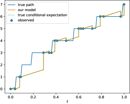
Figure 2: Predicted and true conditional expectation on a test sample of the Poisson point process. All upward movements of the true path are jumps, the slope is only due to the discretization time grid.

8.2 Uncertainty Estimation – Brownian Motion and its Square

We apply NJ-ODE to a Brownian motion $X$ and its square $X^{2}$, as described in Example 5.1, to show that our model can be used to compute the conditional variance, which gives rise to an uncertainty estimate of the prediction. In Figure 3, we show the predictions of the 2-dim process $(X,X^{2})$ as well as the prediction of $X$ together with a confidence region defined as $\hat{\mu}_{t}\pm\hat{\sigma}_{t}$, where $\hat{\mu}_{t}$ is NJ-ODE’s predicted conditional expectation and $\hat{\sigma}_{t}^{2}$ is its predicted conditional variance at time $t$. The evaluation metric on the 2-dimensional dataset becomes smaller than $5\cdot 10^{-5}$.

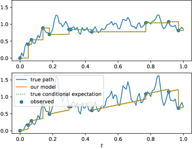
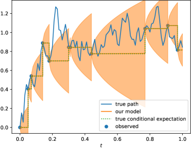
Figure 3: Left: a test sample of a Brownian motion $X$ (top) and its square $X^{2}$ (bottom) together with the predicted and true conditional expectation. Right: the same test sample of the Brownian motion $X$ with a confidence interval given as $\hat{\mu}_{t}\pm\hat{\sigma}_{t}$.

8.3 Path Dependent Process – Fractional Brownian Motion

Table 1: Minimal evaluation metrics on the test set of FBM (with $H=0.05$) within the $200$ epochs of training for different NJ-ODE models.

	NJ-ODE	NJ-ODE (with sig.)	NJ-ODE (with RNN)	PD-NJ-ODE
min. evaluation metric	$8.1\cdot 10^{-2}$	$1.0\cdot 10^{-2}$	$1.1\cdot 10^{-2}$	$0.5\cdot 10^{-2}$

Path dependent processes are one of the main application areas for the extension of NJ-ODE. Here we use a fractional Brownian motion (FBM) with Hurst parameter $H=0.05$, which yields a rough process with high negative auto-correlation (cf. Section 7.4). To show that PD-NJ-ODE performs better than the standard NJ-ODE, we compare them as well as 2 intermediate versions, where once the signature is added as input to NJ-ODE and once a recurrent jump network is used in NJ-ODE. For all 4 models the same architecture is used. The optimal evaluation metric for each of the models is given in Table 1. PD-NJ-ODE achieves the best evaluation metric, for the two intermediate models it is approximately doubled and for NJ-ODE it is about $16$ times larger.
Although our theoretical results imply that the NJ-ODE with signature should be enough, the performance can depend on the truncation level used for the signature input. All truncation levels between $m\in\{1,\dotsc,10\}$ were tested. For $m=1$ and $m=2$ the minimal evaluation metric was $1.1\cdot 10^{-2}$ and $0.6\cdot 10^{-2}$. For all $m\geq 3$, it was $0.5\cdot 10^{-2}$. The computation time grows with increasing truncation level $m$, since it depends on the input dimension of the neural networks which increases according to (8) for growing $m$. Therefore, we choose to use a truncation level of $2$ or $3$ for all of our experiments, since this seems to be a good trade-off between model performance and computation time. Here we report results with $m=3$.
Since truncation levels up to $m=10$ are still rather small, it is not surprising that using the recurrent structure can carry on additional path information that is not covered by the truncated signature and therefore leads to improved quality.
On the other hand these results also show that the recurrent structure alone does not carry all necessary path information. These differences in the quality of the predictions can also be seen in Figure 4.

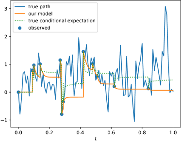
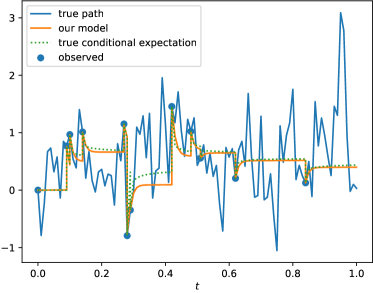
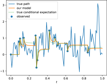
Figure 4: NJ-ODE (top-left), NJ-ODE with signature input (top-right), NJ-ODE with recurrent jump network (bottom-left) and PD-NJ-ODE (bottom-right) on a test sample of a fractional Brownian motion with Hurst parameter $H=0.05$.

8.4 Incomplete Observations – Correlated 2-Dimension Brownian Motion

To test the model on a synthetic dataset with incomplete observations, we consider the example of a 2-dimensional correlated Brownian motion, as described in Section 7.5, with $\alpha^{2}=0.9$. From the discretization grid, we first sample observation times as usual and for each observation time one of the two coordinates is picked at random to be observed (cf. Appendix D.1.3, where $\lambda=0$ is used). The derivations in Section 7.5 show that the incomplete observations also introduce some path dependence. The path-dependent NJ-ODE model achieves a minimal evaluation metric of $5.2\cdot 10^{-3}$ and we see that it reacts well with its prediction of the one coordinate when the other coordinate is observed, even for multiple consecutive observations of the same coordinate (Figure 5).

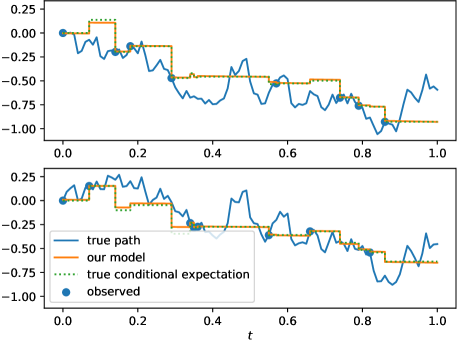
Figure 5: Predicted and true conditional expectation on a test sample of the 2-dimensional correlated Brownian motion (first coordinate plotted on top, second on bottom). The PD-NJ-ODE adjusts its prediction well for both coordinates when observing only one of them.

8.5 Stochastic Filtering of a Brownian Motion with Brownian Noise

PD-NJ-ODE is applied to the stochastic filtering problem that was described in Section 7.6, where $\alpha=1$ and observation probabilities $p_{k}=0.25$, for the $X$-coordinates of the training set, are used. The model achieves a minimal evaluation metric of $5.4\cdot 10^{-4}$ and we see that it learns to use new observations of $Y$ to update the predictions of $X$ (Figure 6).

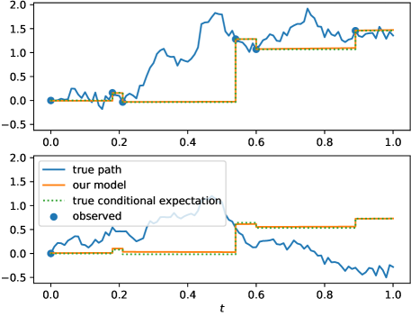
Figure 6: Predicted and true conditional expectation on a test sample of the stochastic filtering dataset. The first coordinate (plotted on top) is the observation process $Y=\alpha X+W$ and the second coordinate (bottom) is the signal process $X$ (which is never observed on test samples).

8.6 Physionet

We test the PD-NJ-ODE model on the extrapolation task of Rubanova et al. (2019) on the PhysioNet Challenge 2012 dataset (Goldberger et al., 2000) and compare it to the results of NJ-ODE. In Table 2 we see that the PD-NJ-ODE outperforms the NJ-ODE. While the results for the PD-NJ-ODE are computed with $1$-hidden layer neural networks with $50$ hidden nodes, compared to $2$-hidden layer networks with $50$ hidden nodes for NJ-ODE, the amount of parameters is much larger, since the signature truncated at level $2$ is used as additional input (for the $41$-dimensional underlying process, this amounts to $1^{\prime}723$ additional inputs). These results suggest that there is some (small) path-dependence in the PhysioNet dataset, which could be dealt with by the PD-NJ-ODE model.

Table 2: Mean and standard deviation of MSE on the test set of physionet. Results of baselines were reported by Rubanova et al. (2019) and Herrera et al. (2021). Where known, the number of trainable parameters is reported.

	Physionet – MSE $(\times 10^{-3})$	# params
RNN-VAE	$3.055\pm 0.145$	-
Latent ODE (RNN enc.)	$3.162\pm 0.052$	-
Latent ODE (ODE enc)	$2.231\pm 0.029$	$163^{\prime}972$
Latent ODE + Poisson	$2.208\pm 0.050$	$181^{\prime}723$
NJ-ODE	1.945 $\pm$ 0.007	$24^{\prime}423$
PD-NJ-ODE	1.930 $\pm$ 0.006	$201^{\prime}691$

8.7 Limit Order Book Datasets

Stock and crypto-currency exchanges use a limit order book (LOB) to track all limit orders of agents who want to buy or sell any of the assets that are traded at the exchange. For each asset, the LOB has a buy and a sell side and for each side lists all the price levels together with the respective order volumes at which the agents would like to buy or sell. The midprice is defined as the mean between the best bid (buy order) and ask (sell order) price. The LOB of level $n\in\mathbb{N}$ is a truncated version of the LOB which only includes the $n$ best (highest) bid and the $n$ best (lowest) ask prices. In the following we always work with LOBs of level $n=10$. Whenever a new order is made or an order is cancelled, the LOB is updated. New limit orders are added to the book, while new market orders are directly executed against the best available limit orders. Hence, LOBs are updated irregularly in time, making them a natural example to apply the PD-NJ-ODE.

We test our model on crypto-currency LOB data. The first dataset (denoted “BTC”) is based on one day of data of the LOB of Bitcoin, which was gratefully provided to us by Covario. The other datasets (denoted “BTC1sec” and “ETH1sec”) are based on roughly 12 days of snapshots of the LOB of Bitcoin (BTC) and Ethereum (ETH) at a frequency of 1 second (once every second the state of the LOB is saved instead of saving it at every update of the book). Using snapshots of the LOB at a predefined frequency usually leads to a loss of information compared to the full LOB. However, these datasets are publicly available (Nielsen, 2021), which is the reason why we include them here. For all datasets, any data point at which the first 10 levels of the LOB did not change compared to the previous one is deleted. The datasets are split into non-overlapping samples, which have $100$ consecutive data points as input and the data point $10$ steps ahead as label to be predicted.

Table 3: Minimal MSEs (smaller is better) during the training of each model (if applicable) are reported for different LOB datasets.

	BTC	BTC1sec	ETH1sec
last observation	$0.11808$	$1350.44$	$2.58909$
best linear regression	$0.12198$	$1355.04$	$2.58253$
PD-NJ-ODE	0.11743	1343.91	2.56636

Table 4: The true mean value and PD-NJ-ODE’s mean predicted value of the midprices $10$ steps ahead for the 3 different datasets and their subsets by labels.

	BTC		BTC1sec		ETH1sec
	true	prediction	true	prediction	true	prediction
overall	$0.01143$	$0.01123$	$-2.40790$	$-2.39125$	$-0.12932$	$-0.10787$
decrease	$-0.41470$	$-0.31175$	$-47.28358$	$-28.80446$	$-2.19563$	$-1.25667$
stationary	$0.08016$	$0.08585$	$-2.75307$	$-3.27602$	$-0.34508$	$-0.36719$
increase	$0.44849$	$0.31417$	$40.63428$	$23.33839$	$2.24031$	$1.30459$

The common task in the literature is to predict price movements, i.e., whether the midprice increases, decreases or stays roughly constant (Tran et al., 2017; Tsantekidis et al., 2017; Dixon et al., 2017; Ntakaris et al., 2018; Passalis et al., 2018; Tsantekidis et al., 2020; Zhang et al., 2019). As a baseline, we use the state-of-the-art DeepLOB model of Zhang et al. (2019), which was shown to outperform many other models.
To compare to these results, we extend the PD-NJ-ODE model by a classifier network, which maps the latent variable $H_{t_{n}}$ after the last data point was processed to the probabilities that the $10$-steps ahead label belongs to one of the classes (increase, decrease, stationary). This classifier network is trained using a cross-entropy loss, first together with the remaining PD-NJ-ODE architecture and afterwards again on its own. We retrain the classifier because the training of the PD-NJ-ODE model is relatively time-consuming, while training the classifier alone is very fast. Since the $50$ epochs for which the PD-NJ-ODE is trained are not sufficient for the classifier to reach its best performance, we retrain it for another $1000$ epochs on its own.

The natural task for our model is the regression problem to forecast the value of the midprice $10$-steps ahead. Due to a lack of baseline models in the literature for this task, we compare the midprice prediction of PD-NJ-ODE to 2 simple baselines. First, we use the midprice of the last observation as prediction for the midprice $10$ steps ahead, i.e., the stationary prediction. And secondly, we fit linear regression models on the entire training data or subsets of it (only midprices and bid/ask prices but no volumes, only midprices, only midprices of last 10 observation dates, only midprice of last observation date). For all datasets, the best liner regression model is the one using only the midprice of the last observation, therefore only results of this model are reported.

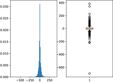
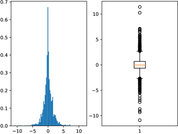
Figure 14: Distribution of the prediction errors of the PD-NJ-ODE model as (density) histogram and boxplot on the BTC1sec (left) and ETH1sec (right) dataset.

In Table 3 we see that in the regression task the PD-NJ-ODE model outperforms the best baseline method by about $0.5\%$ in each of the three datasets. Although this outperformance is relatively small, it is important to note that in both Bitcoin datasets all linear regression models do worse than the stationary prediction and in the Ethereum dataset only the easiest linear model, using only the midprice of the last observation time as predictor, is slightly better than the stationary prediction. In particular this implies that even very easy linear models overfit to the noise in the LOB data. On the contrary, the PD-NJ-ODE model manages to extract at least a little more information from the LOB paths without wrongly adapting to their noise. In Table 4 we show our model’s mean predicted value and the true mean value of the midprice $10$ steps ahead for the entire datasets and for the subset of the three different labels. Taking the means is a good way to average out the random noise of the samples. But, at the same time, also some true information is averaged out (see for example the difference between overall mean and the means of the three labels). For all three datasets we see that the overall mean prediction is relatively close to the true mean, while the absolute values of the mean predictions for decrease and increase labels are significantly smaller than the true ones. This can be explained with the boxplot of the prediction errors (i.e., the differences between predicted values and the respective true values) shown in Figure 7 for the BTC dataset and in Figure 14 in the Appendix for the other two datasets. Although the distributions are concentrated closely around $0$, there are many large outliers on both sides, which increase the true absolute means for decrease and increase labels. On the other hand, the PD-NJ-ODE model seems to learn the main behaviour without overfitting to these large valued outliers, which keeps the predicted absolute means smaller in those two groups. In particular, this suggests that the PD-NJ-ODE is a robust and flexible model at the same time.

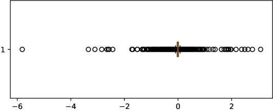
Figure 7: Boxplot of the prediction errors of the PD-NJ-ODE model on the BTC dataset.

The results of the classification task for the three datasets are shown in Table 5, where we compare the weighted F1-scores of the models, as it was done by Zhang et al. (2019). For the two Bitcoin datasets, the PD-NJ-ODE (with retrained classifier) and DeepLOB yield very similar results. On the Ethereum dataset, our model achieves slightly better results than on “BTC1sec”, while the DeepLOB model performs significantly worse, for which we do not have an explanation. Overall we conclude that even though classification is not the core task of our model, the results are very promising already with a simple classifier network that is added on top of the PD-NJ-ODE model.

Table 5: Maximal F1-scores (in $\%$, larger is better) during the training of each model are reported for different LOB datasets.

	BTC	BTC1sec	ETH1sec
DeepLOB	$61.59$	52.24	$44.97$
PD-NJ-ODE (no retraining)	$52.34$	$52.02$	$52.48$
PD-NJ-ODE (classifier retrained)	62.06	no improvement	54.08

9 Conclusion

We extended the NJ-ODE model to work for much more general datasets and settings. In Herrera et al. (2021) there were examples for which NJ-ODE worked well empirically, although they were not covered by the theoretical settings. Here, we brought the theoretical and empirical results to the same level, by giving the weakest possible constraints on the data process such that PD-NJ-ODE can be applied successfully. Indeed, if the continuous differentiability of the conditional expectation is not satisfied, it is clear that the proposed framework cannot approximate it arbitrarily well, since neural networks cannot approximate the corresponding functions arbitrarily well. On the other hand, if the integrability assumption is not satisfied, the loss function is not well defined. Moreover, we showed empirically, using multiple synthetic datasets, that the PD-NJ-ODE truly works in all of those more complicated settings that are permitted by the theoretical results now. Finally, the application of PD-NJ-ODE to limit order book data had very promising results, which will be elaborated further in future work.

Appendix

Appendix A A Generalized Version of the Filtering Problem

The filtering problem of Section 6.1 can be generalized in two simple ways that are supported by the PD-NJ-ODE model without the need of any additional assumptions. On the one hand, it is not necessary that the $Y$-coordinates are observed completely. It is not even necessary that every $Y$-coordinate might be observed with positive probability at every observation time. To satisfy our assumptions, we only assume that always the same coordinates of $Y_{0}$ are observed. This generalisation corresponds to the possibility that certain sensors might suffer of malfunction or could be shut off from time to time. On the other hand, some of the $X$-coordinates might be observed from time to time, which means that the ground truth is sometimes (partly) observable. Again, to satisfy our assumptions, we assume that always the same coordinates of $\varphi(X_{0})$ are observed. Without loss of generality we also assume that at each observation time, at least one coordinate is observed, since otherwise it would not be an observation time and could be deleted. However, it is for example possible that only some $X$-coordinates and no $Y$-coordinates are observed at certain observation times.

Let $\mathcal{Z}_{t}$ be the $\sigma$-algebra describing the currently available information (of evaluation samples). Moreover, let $\varphi:\mathbb{R}^{d_{X}}\to\mathbb{R}^{d_{\varphi}}$ be any integrable measurable function that can be evaluated with incomplete observations (e.g. a function that is applied element-wise).

Remark A.1.

In the case that the $X$-coordinates are never observed in the evaluation samples, $\varphi$ can be any integrable measurable function.

Then, the filtering problem amounts to computing

$$\mathbb{E}[\varphi(X_{t})\,|\,\mathcal{Z}_{t}].$$

To train the PD-NJ-ODE model to approximate this random function, we generate a training dataset similarly as in Section 6.2, with the difference that the generated observation mask has the probability $p_{k}\in(0,1)$ for $k\geq 1$ for each coordinate of $M_{k}$ to be $1$ individually. At $t=0$ exactly those coordinates of $M_{0}$ corresponding to the coordinates of $(\varphi(X_{0}),Y_{0})$ that are always observed, are $1$.

Remark A.2.

In the case that the $X$-coordinates are never observed in the evaluation samples, the coordinates of $M_{k}$, $k\geq 1$, corresponding to $X$ are generated either all $0$ or all $1$ simultaneously (as before), while the coordinates corresponding to $Y$ are sampled individually.

Then the following results follow similarly as Corollary 6.2.

Corollary A.3.

Assume that the training samples are generated as described above and that $Z=(\varphi(X),Y)$ satisfies Assumptions 4 and 5. Let $\theta^{\min}_{m,N}\in\Theta^{\min}_{m,N}:=\arg\inf_{\theta\in\Theta_{m}}\{\hat{\Phi}_{N}(\theta)\}$ for every $m,N\in\mathbb{N}$. Then, one can define an increasing sequence $(N_{m})_{m\in\mathbb{N}}$ in $\mathbb{N}$ such that for every $1\leq k\leq K$ the following statements hold.

1. $G^{\theta_{m,N_{m}}^{\min}}$ converges to $\hat{Z}=(\widehat{\varphi(X)},\hat{Y})$ in the metric $d_{k}$ as $m\to\infty$.

In the case that the $X$-coordinates are never observed in the evaluation samples, we write $\mathcal{Y}_{t}=\mathcal{Z}_{t}$ (even though here the $Y$-coordinates might not be observed completely). Then the following statements hold.

1. $G^{\theta_{m,N_{m}}^{\min}}$ converges to $\hat{Z}$ in the metric $\tilde{d}_{k}$ as $m\to\infty$.

2. It holds that

   $$\tilde{d}_{k}\left(G^{\theta_{m,N_{m}}^{\min}}(Z),G^{\theta_{m,N_{m}}^{\min}}(Y)\right)=\tilde{d}_{k}\left(\hat{Z},\left(\mathbb{E}[Z\,|\,\mathcal{Y}_{t}]\right)_{t\in[0,T]}\right)=0.$$

Appendix B Additional Examples of Processes Satisfying the Assumptions

B.1 Stochastic Functional Differential Equations

Following the definitions in Cohen & Elliott (2015, Section 16.2), let $\mathcal{D}$ be the space of càdlàg adapted processes on $\mathbb{R}^{d}_{X}$ and $S^{p}\subseteq\mathcal{D}$ for $2\leq p<\infty$, the set of all processes $X\in\mathcal{D}$ for which

$$\|X\|_{S^{p}}:=\|X^{\star}_{T}\|_{L^{p}}=\mathbb{E}[(X_{T}^{\star})^{p}]^{1/p}<\infty,$$

where $X^{\star}=\max_{i}\{X_{i}^{\star}\}$ for multidimensional processes and where we use the finite time horizon $T$ instead of $\infty$. We look at functions $f:\Omega\times[0,T]\times\mathcal{D}\to\mathbb{R}^{u\times v},(\omega,t,X)\mapsto f(\omega,t,X)=f(X)$ that are uniformly Lipschitz, i.e., there exists some $L\in\mathbb{R}$ such that for any $X,Y\in\mathcal{D}$ and $t\in[0,T]$,

$$(f(X)-f(Y))^{\star}_{t}\leq L(X-Y)^{\star}_{t-}.$$ (29)

For such functions we write $f\in\operatorname{Lip}(L)$. It is clear from this definition that $f(X)_{t}$ only depends on $(X_{s})_{0\leq s\leq t}$. Moreover, for such functions we have that $\|f(X)-f(Y)\|_{S^{p}}\leq L\|X-Y\|_{S^{p}}$.

Let $2\leq p<\infty$, $d_{W}\in\mathbb{N}$ and let $(W_{t})_{t\in[0,T]}$ be a $d_{W}$-dimensional Brownian motion on the probability space $(\Omega,\mathcal{F},\mathbb{F}:=(\mathcal{F}_{t}\}_{0\leq t\leq T},\mathbb{P})$. We assume that the stochastic process $X:=(X_{t})_{t\in[0,T]}$ is defined as the continuous solution of the stochastic functional differential equation

$$dX_{t}=\mu\left(\omega,t,X\right)dt+\sigma\left(\omega,t,X\right)d{W}_{t},=\mu(X)_{t}dt+\sigma(X)_{t}dW_{t}$$ (30)

for all $0\leq t\leq T$ with (random) starting point $X_{0}$ taking values in $\mathbb{R}^{d_{X}}$ such that $\|X_{0}\|_{L^{p}}<\infty$, drift function $\mu:\Omega\times[0,T]\times\mathcal{D}\to\mathbb{R}^{d_{X}}$ and diffusion function $\sigma:\Omega\times[0,T]\times\mathcal{D}\to\mathbb{R}^{d_{X}\times d_{W}}$. We assume that $\mu$ and $\sigma$ are uniformly Lipschitz in the sense of (29) and that there exists a constant $C>L$ such that $\|\mu(0)\|_{S^{p}}+\|\sigma(0)\|_{S^{p}}<C$. Moreover, we assume that we always observe all coordinates of $X$ simultaneously. These assumptions imply that $\mu$ and $\sigma$ have linear growth,

$$\|\mu(X)\|_{S^{p}} =\|\mu(0)\|_{S^{p}}+(\|\mu(X)\|_{S^{p}}-\|\mu(0)\|_{S^{p}})\leq\|\mu(0)\|_{S^{p}}+\|\mu(X)-\mu(0)\|_{S^{p}}$$

$$\leq\|\mu(0)\|_{S^{p}}+L\|X\|_{S^{p}}\leq C(1+\|X\|_{S^{p}}),$$

and similar for $\sigma$.

It is easy to see that $(W_{t})_{0\leq t\leq T}$ and $(t)_{0\leq t\leq T}$ are both $\alpha$-sliceable for any $\alpha>0$ (Cohen & Elliott, 2015, Definition 16.3.8), in fact even with deterministic stopping times. Therefore, Cohen & Elliott (2015, Lemma 16.3.10) implies that there exists a unique solution to (30) and that this solution satisfies

$$\|X\|_{S^{p}}\leq\tilde{C}(\|X_{0}\|_{L^{p}}+\|\mu(0)\|_{S^{p}}+\|\sigma(0)\|_{S^{p}}),$$

for some $\tilde{C}$ depending only on $L$ and $W$. In particular, we can choose $C$ such that $\|X\|_{S^{p}}<C$. This implies integrability of the drift and diffusion component

$$\mathbb{E}\left[\int_{0}^{T}|\mu(X)_{t}|+|\sigma(X)_{t}|^{2}\,dt\right] =\int_{0}^{T}\mathbb{E}\left[|\mu(X)_{t}|+|\sigma(X)_{t}|^{2}\right]\,dt$$

$$\leq\int_{0}^{T}\left(\|\mu(X)\|_{S^{p}}+\|\sigma(X)\|_{S^{p}}^{2}\right)\,dt$$

$$\leq 2TC^{2}(1+C)^{2},$$ (31)

where we used Fubini’s Theorem in the first and Hölder’s inequality in the second step.

(B.1) yields that the process

$$\tilde{M}_{t}:=\int_{0}^{t}\sigma(s,X_{s},X_{<s})d{W}_{s},\quad 0\leq t\leq T,$$

is a square integrable martingale by Protter (2005, Lemma before Thm. 28, Chap. IV) since the Brownian motion ${W}$ is square integrable with $d[W^{i},W^{j}]_{t}=\delta_{i,j}dt$. Using the martingale property of $\tilde{M}$ and the tower property for $\mathcal{A}_{\tau(t)}\subseteq\mathcal{F}_{\tau(t)}$, we have ($\tilde{\omega}$-wise) for every $t\in[0,T]$,

$$\hat{X}_{t} =\mathbb{E}_{\mathbb{P}}\left[\left(X_{t}-X_{\tau(t)}\right)+X_{\tau(t)}|\mathcal{A}_{\tau(t)}\right]$$

$$=X_{\tau(t)}+\mathbb{E}_{\mathbb{P}}\left[\int_{\tau(t)}^{t}\mu(X)_{r}\,dr|\mathcal{A}_{\tau(t)}\right]+\mathbb{E}_{\mathbb{P}}\left[\int_{\tau(t)}^{t}\sigma(X)_{r}\,dW_{r}|\mathcal{A}_{\tau(t)}\right]$$

$$=X_{\tau(t)}+\int_{\tau(t)}^{t}\mathbb{E}_{\mathbb{P}}\left[\mu(X)_{r}\,|\mathcal{A}_{\tau(t)}\right]dr+\mathbb{E}_{\mathbb{P}}\left[\mathbb{E}_{\mathbb{P}}\left[M_{t}-M_{\tau(t)}|\mathcal{F}_{\tau(t)}\right]|\mathcal{A}_{\tau(t)}\right]$$

$$=X_{\tau(t)}+\int_{\tau(t)}^{t}\mathbb{E}_{\mathbb{P}}\left[\mu(X)_{r}\,|\mathcal{A}_{\tau(t)}\right]dr,$$ (32)

where we used Fubini’s theorem (for conditional expectation) in the second last step, which is justified because of (B.1). Let us define $\Delta:=\left\{(t,r)\in[0,T]^{2}|t+r\leq T\right\}$ and the function

$$\tilde{\mu}:\Delta\times BV([0,T]) \rightarrow\mathbb{R}^{d_{X}}$$

$$((t,r),\xi) \mapsto\mathbb{E}_{\mathbb{P}}\left[\mu(\omega,t+r,X)|\tilde{X}^{\leq t}=\xi\right],$$

then the Doob-Dynkin Lemma (Taraldsen, 2018, Lemma 2) implies that we can rewrite (32) as

$$\hat{X}_{t}=X_{\tau(t)}+\int_{\tau(t)}^{t}\tilde{\mu}\left(\tau(t),r-\tau(t),\tilde{X}^{\leq\tau(t)}\right)dr.$$ (33)

To satisfy Assumption 4, we need that $\tilde{\mu}$ is continuous. While this might not be true in general, the following examples give cases where this can be shown.

Example B.1.

Under the additional assumption that $\mu$ and $\sigma$ only depend on the current value of $X$ and not its entire path, Gubinelli (2016, Theorem 8) together with Herrera et al. (2021, Proposition B.4) prove that $\tilde{\mu}$ is continuous. Importantly, here we do not need the boundedness assumption for $\mu$ nor the integrability assumption for $\sigma$, hence this generalizes the example from Section 7.1 as described in Remark 7.2. Notice that by adding further factors to the state space of $X$, which are unobserved and which follow a Markovian dynamics satisfying mild regularity conditions, we can include many path dependence structures of the drift and therefore also obtain continuous dependence of $\tilde{\mu}$ (with respect to those factors) in an analogous manner.

Example B.2.

If we additionally assume that $\mu(X)_{t}=\alpha X_{t}+\beta$ for some $\alpha,\beta\in\mathbb{R}$, i.e., linear in the current value of $X$, while $\sigma$ can be general and path dependent, we can show that $\tilde{\mu}$ is continuous. Indeed, then it follows from (32) that

$$\mathbb{E}_{\mathbb{P}}\left[X_{t}\,|\mathcal{A}_{\tau(t)}\right]=X_{\tau(t)}+\int_{\tau(t)}^{t}\left(\alpha\mathbb{E}_{\mathbb{P}}\left[X_{r}\,|\mathcal{A}_{\tau(t)}\right]+\beta\right)dr.$$ (34)

(34) is equivalent to the ordinary differential equation

$$\begin{split}y^{\prime}(t)&=\alpha y(t)+\beta,\quad t\geq\tau(t),\\ y(\tau(t))&=y_{\tau}:=X_{\tau(t)},\end{split}$$

by defining $y(r):=\mathbb{E}_{\mathbb{P}}\left[X_{r}\,|\mathcal{A}_{\tau(t)}\right]$ for $r\geq\tau(t)$. The unique solution to this initial value problem is given by $y(t)=-\frac{\beta}{\alpha}+\left(\frac{\beta}{\alpha}+y_{\tau}\right)e^{\alpha(t-\tau)}$ hence the conditional expectation between $\tau(t)$ and the next observation is given by

$$\mathbb{E}_{\mathbb{P}}\left[X_{r}\,|\mathcal{A}_{\tau(t)}\right]=F(r,\tau,\tilde{X}^{\leq\tau})=-\frac{\beta}{\alpha}+\left(\frac{\beta}{\alpha}+X_{\tau(t)}\right)e^{\alpha(t-\tau)},$$

which is continuous and differentiable in $t$ leading to

$$\tilde{\mu}\left(\tau,r-\tau,\tilde{X}^{\leq\tau}\right)=\alpha\mathbb{E}_{\mathbb{P}}\left[X_{r}\,|\mathcal{A}_{\tau}\right]+\beta=\left(\beta+\alpha X_{\tau}\right)e^{\alpha(r-\tau)}=f(r,\tau,\tilde{X}^{\leq\tau})=\frac{\partial}{\partial r}F(r,\tau,\tilde{X}^{\leq\tau}).$$

B.2 Predicting a Time-Lagged Version of an Observed Process

Let $(X_{t})_{t\geq 0}$ be a $1$-dimensional stochastic process, let $\alpha>0$ and define $Y_{t}:=X_{t-\alpha}$, with the convention that $X_{t}=0$ for all $t\leq 0$. If $X$ satisfies the integrability assumption, then also $Z:=(X,Y)$ does. We are interested in (optimally) predicting $Y$ given observations of $X$. This problem is somehow related to the filtering problem, in the sense that one only observes one process (here $X$) and wants to make predictions for the other process (here $Y$). In contrast to the filtering problem, the observations of $X$ also show up as observations of $Y$ after an elapse time of $\alpha$. However, it is clear that this observation structure does not satisfy our assumption that every coordinate is observed with positive probability at any observation time. This is a problem, because the (theoretical) loss function does not have a unique minimizer any more. The first coordinate of a minimiser still has to be given by the conditional expectation (since the assumptions hold for this coordinate), however, its second coordinate only has to equal the observations of the first coordinate after an elapse time of $\alpha$ (i.e., at times $t_{i}+\alpha$, where $t_{i}$ are the observation times of the first coordinate). Whatever the second coordinate does in between these points does not change the loss, since no observations are made there. We can deal with this problem similarly as in the filtering framework, if we assume that we can sample a more general training dataset, where observations of $Y$ are possible in between the observations of $X$. Importantly, such observations of $Y$ only happen at times $t$ for which $t<\tau_{X}(t)+\alpha$, where $\tau_{X}(t)$ is the last observation time of $X$ before $t$, since otherwise the observation of $Y$ would impact the prediction of $X$. If for any $t\in[0,T]$ with $\tau_{X}(t)\leq t<\tau_{X}(t)+\alpha$ the probability of observing $Y_{t}$ is in $(0,1)$, then the minimizer of the loss function is again uniquely given by the conditional expectation process. As in the filtering problem, the trained model can be evaluated on the original samples, where only the process $X$ is observed.

Example B.3 (Brownian Motion and its Time-Lagged Version).

Let $X$ be a $1$-dimensional Brownian motion. Then $X$ satisfies $\mathbb{E}[(X^{\star}_{T})^{p}]<\infty$ for every $1\leq p<\infty$ (cf. Cohen & Elliott (2015, Lemma 16.1.4)) and therefore also $Z$. The analytic expression of the conditional expectation can be derived as follows. For $X$ it is simply given by its last observation (cf. Section 7.5). For $Y$ we have to distinguish between 3 cases. If $t\leq\alpha$, then $\mathbb{E}[Y_{t}|\mathcal{A}_{t}]=0$, since $Y_{t}=X_{t-\alpha}=0$. If $t\geq\tau_{X}(t)+\alpha$, i.e., if the last observation of $X$ was longer ago than $\alpha$, then (cf. Cohen & Elliott (2015, Lemma 16.1.4))

$$\mathbb{E}[Y_{t}|\mathcal{A}_{t}]=\mathbb{E}[(X_{t-\alpha}-X_{\tau_{X}(t)})+X_{\tau_{X}(t)}|\mathcal{A}_{t}]=X_{\tau_{X}(t)}.$$

Finally, if $h<t<\tau_{X}(t)+\alpha$, then $s:=t-\alpha$ lies between two observation times of $X$ (which both happened before $t$). Let us assume that there are $k$ observations until $t$ and that $1\leq\ell\leq k$ is such that $t_{0}<\dotsb<t_{\ell-1}<s<t_{\ell}<\dotsb<t_{k}$. Then $v:=(X_{s},X_{t_{1}},\dotsc,X_{t_{k}})$ is a Gaussian vector with $v\sim N(0,\tilde{\Sigma})$, where

$$\tilde{\Sigma}:=\begin{pmatrix}\tilde{\Sigma}_{11}&\tilde{\Sigma}_{12}\\ \tilde{\Sigma}_{21}&\tilde{\Sigma}_{22}\end{pmatrix},$$

with $\tilde{\Sigma}_{11}=\operatorname{Var}(X_{s})=s\in\mathbb{R}$, $\tilde{\Sigma}_{12}=\tilde{\Sigma}_{21}^{\top}=(t_{1},\dotsc,t_{\ell-1},s,\dotsc,s)\in\mathbb{R}^{1\times k}$ and $\tilde{\Sigma}_{22}\in\mathbb{R}^{k\times k}$, given by $(\tilde{\Sigma}_{22})_{i,j}=t_{\min(i,j)}$. Note that this follows from the definition of a Brownian motion, which implies that $\operatorname{Cov}(X_{a},X_{b})=\min(a,b)$. Then, the conditional distribution of $(X_{s}\,|\,X_{t_{1}},\dotsc,X_{t_{k}})$ is again normal with mean $\hat{\mu}:=\tilde{\Sigma}_{12}\tilde{\Sigma}_{22}^{-1}(X_{t_{1}},\dotsc,X_{t_{k}})^{\top}$ and variance $\hat{\Sigma}:=\tilde{\Sigma}_{11}-\tilde{\Sigma}_{12}\tilde{\Sigma}_{22}^{-1}\tilde{\Sigma}_{21}$ (Eaton, 2007, Proposition 3.13). In particular, we have

$$\mathbb{E}[Y_{t}|\mathcal{A}_{t}]=\mathbb{E}[X_{s}|X_{t_{1}},\dotsc,X_{t_{k}}]=\hat{\mu}.$$

A direct computation shows that

$$(\tilde{\Sigma}_{22}^{-1})_{i,j}=\begin{cases}(t_{i}-t_{i-1})^{-1}+(t_{i+1}-t_{i})^{-1},&\text{if }i=j<k,\\ (t_{k}-t_{k-1})^{-1},&\text{if }i=j=k,\\ -(t_{i}-t_{j})^{-1},&\text{if }i=j+1,\\ -(t_{j}-t_{i})^{-1},&\text{if }j=i+1,\\ 0,&\text{otherwise},\end{cases}$$

with which we can compute that

$$\hat{\mu}=\tilde{\Sigma}_{12}\tilde{\Sigma}_{22}^{-1}(X_{t_{1}},\dotsc,X_{t_{k}})^{\top}=X_{t_{\ell-1}}+(X_{t_{\ell}}-X_{t_{\ell-1}})\frac{s-t_{\ell-1}}{t_{\ell}-t_{\ell-1}}.$$

In particular this means that the conditional expectation between any two observations is given by the linear interpolation of these observations.

B.3 Chaotic Systems

A chaotic system is a deterministic dynamical system which is sensitive to initial conditions, topologically transitive and has dense periodic orbits (Hasselblatt & Katok, 2003). In particular, although the system is in principle deterministic, small changes in the initial condition lead to vastly different trajectories of the system. A chaotic system, where the initial point is chosen from some distribution supported on a compact set, with discrete observation times (where the initial point is observed completely) falls into our framework and satisfies Assumptions 4 and 5, if it has $C^{1}$ trajectories. Indeed, since $X_{0}$ is observed, the conditional expectation is given by the deterministic trajectory starting at $X_{0}$. Hence, Assumption 4 is satisfied. Moreover, since the trajectories are continuous as functions of the initial point and time, they are bounded on $\operatorname{supp}(X_{0})\times[0,T]$ (since a continuous function on a compact subset is bounded) which implies that also Assumption 5 is satisfied.

Example B.4 (Double Pendulum).

One of the best known examples of a chaotic system is a double pendulum as depicted in Figure 8. Here, we shortly explain its dynamics following Svirin (2009).

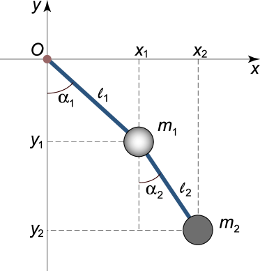
Figure 8: A schematic representation of a double pendulum. Picture copied from Svirin (2009).

The dynamical system is at any point determined completely by a $4$-dimensional state vector $(\alpha_{1},\alpha_{2},p_{1},p_{2})$, where $(\alpha_{1},\alpha_{2})$ determine the current position of both pendulums and $(p_{1},p_{2})$ are the so-called generalized momenta, which are related to the velocities of both pendulums. The differential equation describing the dynamics of this state vector is

$$\alpha_{1}^{\prime} =\frac{p_{1}l_{2}-p_{2}l_{1}\cos(\alpha_{1}-\alpha_{2})}{l_{1}^{2}l_{2}A_{0}},$$

$$\alpha_{2}^{\prime} =\frac{p_{2}(m_{1}+m_{2})l_{1}-p_{1}m_{2}l_{2}\cos(\alpha_{1}-\alpha_{2})}{m_{2}l_{1}l_{2}^{2}A_{0}},$$

$$p_{1}^{\prime} =-(m_{1}+m_{2})gl_{1}\sin(\alpha_{1})-A_{1}+A_{2},$$

$$p_{2}^{\prime} =-m_{2}gl_{2}\sin(\alpha_{2})+A_{1}-A_{2},$$

where

$$A_{0} =[m_{1}+m_{2}\sin^{2}(\alpha_{1}-\alpha_{2})],$$

$$A_{1} =\frac{p_{1}p_{2}\sin(\alpha_{1}-\alpha_{2})}{l_{1}l_{2}A_{0}},$$

$$A_{2} =\frac{[p_{1}^{2}m_{2}l_{2}^{2}-2p_{1}p_{2}m_{2}l_{1}l_{2}\cos(\alpha_{1}-\alpha_{2})+p_{2}^{2}(m_{1}+m_{2})l_{1}^{2}]\sin(2(\alpha_{1}-\alpha_{2}))}{2l_{1}^{2}l_{2}^{2}A_{0}^{2}},$$

and $g$ is the gravitational acceleration constant. As initial points $X_{0}$ we only consider positions where the double pendulum is straight, i.e., both pendulums have the same angle $\alpha_{1}=\alpha_{2}$ and the generalized momenta $p_{1},p_{2}$ are $0$. In particular, we can therefore sample the initial point by sampling $\alpha$ from some distribution on $[0,2\pi]$.

Appendix C Additional Experiments

C.1 Observation Intensity Depending on the Underlying Process

For a Black–Scholes model $X$, we use the following method to randomly sample observation times. As usual, the process is sampled on a grid with step size $0.01$ and for each of the grid points an independent Bernoulli random variable is drawn to determine whether it is used as observation time or not (cf. Appendix D.1.3). The only difference is that the success probability of the Bernoulli random variable is $p=0.05+0.4\tanh(|X_{t}|/10)$, where $X_{t}$ is the value of the process at the given grid point. We note that this example is not covered by the extended setting of Andersson et al. (2023). Nevertheless, the PD-NJ-ODE model applied to this dataset learns to correctly predict the process (Figure 9) achieving a minimal evaluation metric of $6.2\cdot 10^{-4}$.

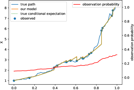
Figure 9: Predicted and true conditional expectation on a test sample of the Black–Scholes dataset, where the observation intensity depends on the values of the process.

C.2 Predicting a Time-Lagged Brownian Motion

To test how well the PD-NJ-ODE model performs in storing information about past events and reusing it at a later time, we apply it to a dataset where the second coordinate is a time-lagged version of the first coordinate, as described in Example B.3, where $\alpha=0.19$. This learning problem is complicated, since the model needs to learn to store past observations of $X$ (together with their observation times) and to decide which of them to use to predict $Y$ depending on their observation times and the current time. Moreover, the model needs to learn to distinguish when a new observation of $X$ changes the current prediction of $Y$ (i.e., when the previous observation of $X$ is longer ago than $\alpha$) and when it does not. Therefore, it is not surprising that the model has some difficulties learning the correct predictions, which is also reflected in the relatively high value $1.0\cdot 10^{-3}$ of the minimal evaluation metric. Nevertheless, we see in Figure 10 that the model learns to approximate the correct behaviour.

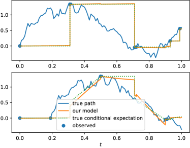
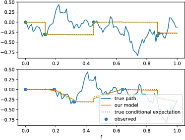
Figure 10: Predicted and true conditional expectation on two test samples of the dataset, where the first coordinate (plotted on top) is a Brownian motion $X$ and the second coordinate (bottom) is its time-lagged version with lag $\alpha=0.19$.

C.3 Chaotic System – Double Pendulum

We apply the PD-NJ-ODE to a Double Pendulum, as described in Example B.4, where we choose $m_{1}=m_{2}=l_{1}=l_{2}=1$ and sample the initial angle for the starting point $X_{0}$ from $\alpha\sim N(\pi,0.2^{2})$, i.e., normally distributed around to highest point the Pendulum could reach. In the generated dataset, we always observe $X_{0}$ and always have complete observations. The PD-NJ-ODE model achieves a minimal evaluation metric of $5.1\cdot 10^{-2}$. In particular we see that it learns to predict the deterministic dynamics of the chaotic system well, even though not free of error. At new observations, the prediction error gets reverted (Figure 11 left). If only the initial point is observed, the error grows over time (Figure 11 right). We note that for chaotic system dataset it is of high importance to chose the step size in the dataset small enough, such that the model can see and learn the entire dynamic (cf. Appendix D.8).

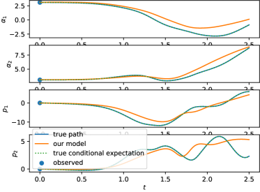
Figure 11: Predicted conditional expectation on two test samples of the Double Pendulum dataset. In the sample on the left, new observations are made over time, such that the model can revert its error. In the sample on the right, only the initial point is observed, which leads to a growing error over time. Since the system is deterministic, the true conditional expectation coincides with the true path.

Appendix D Experimental Details

D.1 Implementation Details

D.1.1 Differences between the Implementation and the Theoretical Description of the PD-NJ-ODE

Below we list all differences between the theoretical description of the PD-NJ-ODE and our implementation of it that can be found at https://github.com/FlorianKrach/PD-NJODE.

• The bounded output neural networks (cf. Definition 3.12) $f_{\theta_{1}}$ and $\rho_{\theta_{2}}$ in (9) needed to derive our theoretical results are replaced by standard neural networks (without the bound from Definition 3.12) in our implementation.

• For the neural network $\rho_{\theta_{2}}$ we use as additional inputs at an observation time $t_{i}$ the self-imputed observation $M_{t_{i}}\odot X_{t_{i}}+(1-M_{t_{i}})\odot Y_{t_{i}}$ and the mask $M_{t_{i}}$. Moreover, the user can choose whether to use time as input, which consists of the current time $t_{i}$ and the previous observation time $t_{i-1}$, and whether to use a recurrent structure by using $H_{t_{i}-}$ as input.

• For the neural network $f_{\theta_{1}}$ we use as additional input for times $t_{i}<t<t_{i+1}$ either the last self-imputed observation $M_{t_{i}}\odot X_{t_{i}}+(1-M_{t_{i}})\odot Y_{t_{i}}$ or the models prediction $Y_{t_{i}}$ at the last observation time (it is the user’s choice which one is used). Moreover, the user can choose whether a $\tanh$ should be applied (element-wise) to the inputs before passing them to the network, such that they lie within $[-1,1]$.

• For both networks $f_{\theta_{1}}$ and $\rho_{\theta_{2}}$ one can choose to use the coordinate-wise last observation times instead of the overall last observation time $\tau$ for the time input.

• The user can choose whether to use a residual connection from input to output for the networks $\rho_{\theta_{2}}$ and $\tilde{g}_{\tilde{\theta}_{3}}$. In the case that a recurrent network is used for $\rho_{\theta_{2}}$, no residual connection is added to it.

• The user can choose whether to use the signature as input for $f_{\theta_{1}}$ and $\rho_{\theta_{2}}$ and up to which truncation level. We directly compute the signature $\pi_{m}(\tilde{X}^{\leq\tau(t)})$ instead of $\pi_{m}(\tilde{X}^{\leq\tau(t)}-X_{0})$ and before computing the signature we add the current time as additional coordinate to $\tilde{X}^{\leq\tau(t)}$.

• The user can choose which architectures to use for the neural networks $f_{\theta_{1}}$, $\rho_{\theta_{2}}$ and $\tilde{g}_{\tilde{\theta}_{3}}$.

• Through the choices whether to use a recurrent structure for $\rho_{\theta_{2}}$ and whether to use the signature as input, the PD-NJ-ODE or the NJ-ODE or the 2 intermediate version can be used. Whenever we speak of the PD-NJ-ODE model we use the signature and the recurrent structure.

• The user can choose to use gradient clipping or output clamping, which is not done by default.

• The solution to the SDE (9) is approximated with the Euler method for some step size $\Delta t$.

• Since the $2$-norms appearing in the objective functions (10), (11), (12) involve computing a square-root, which leads to differentiability issues at $0$, we add a small regularizing constant ($\epsilon=10^{-10}$) to the quantities in the square-roots.

D.1.2 Remarks on the Signature

First we note that the “not-tree-like” condition is easily fulfilled in practice by having a monotonously increasing coordinate in the data. To this end, we concatenate the current time as additional dimension to the data, which is standard procedure when working with signatures (see for example Fermanian (2020)). If the function to be learnt in Theorem 3.7 depends significantly on higher degree terms, and the truncation level is chosen too low, some information will inevitably be lost. For a more elaborate setup, Bonnier et al. (2019) discuss methods to reduce this issue by applying an augmentation to the original data stream before computing the signature. In our applications, we deal with this issue in another way. We use a recurrent structure, which can learn to extract and store certain path-dependent feature of the data. In particular, this could learn to approximate some higher degree term of the signature, which carries significant information

To actually compute the signature (of the interpolated paths we consider), multiple python packages are available, as for example ESig, iisignature and signatory. For our implementation, we use the great iisignature package implemented by Reizenstein & Graham (2018).

D.1.3 Synthetic Datasets

We use the same method to generate datasets as in Herrera et al. (2021). In particular, if not mentioned otherwise, we consider the time interval $[0,1]$, i.e., $T=1$, and a discretization time grid with step size $0.01$ which leads to $101$ time points on this interval. For each path $i$ and each of these time points $t$, an independent Bernoulli random variable $O_{i,t}\sim Bernoulli(p)$ is drawn and the time point is used as observation time if $O_{i,t}=1$. Our standard choice for the success probability is $p=0.1$. The paths themselves are sampled by either using a closed form method if available or the euler scheme adapted to the discretization time grid. The standard choice is to sample a set of $20^{\prime}000$ paths which is split into $80\%$ training set and $20\%$ test set.

For each of the observation times (where $O_{i,t}=1$) of synthetic datasets with incomplete observations (masked data) first an independent random variable $N_{i,t}\sim 1+Poisson(\lambda)$ is drawn, which specifies the amount of coordinates observed at this time. Then $\min(d_{X},N_{i,t})$ coordinates are drawn at random (without replacement) from the set of all coordinates, to be the observed ones. If $\lambda=0$, then exactly one (randomly chosen) coordinate is observed at each observation time.

D.1.4 Training

We always use the Adam optimizer with the standard choices $\beta=(0.9,0.999)$ and weight decay of $0.0005$. If not mentioned otherwise, our standard choice for the learning rate is $0.001$, a dropout rate of $0.1$ is used for every layer and training is performed with a mini-batch size of $200$ for $200$ epochs.

D.1.5 Objective Function

The (original) loss function (10),

$$\Psi:\mathbb{D}\to\mathbb{R},Z\mapsto\Psi(Z):=\mathbb{E}_{\mathbb{P}\times\tilde{\mathbb{P}}}\left[\frac{1}{n}\sum_{i=1}^{n}\left(\left\lvert M_{t}\odot(X_{t_{i}}-Z_{t_{i}})\right\rvert_{2}+\left\lvert M_{t}\odot(Z_{t_{i}}-Z_{t_{i}-})\right\rvert_{2}\right)^{2}\right],$$

uses the distance between the prediction before and after the jump, to make the neural ODE learn the correct behaviour between the jumps. In contrast, the equivalent loss function (cf. Remark 4.8),

$$\tilde{\Psi}:\mathbb{D}\to\mathbb{R},Z\mapsto\Psi(Z):=\mathbb{E}_{\mathbb{P}\times\tilde{\mathbb{P}}}\left[\frac{1}{n}\sum_{i=1}^{n}\left(\left\lvert M_{t}\odot(X_{t_{i}}-Z_{t_{i}})\right\rvert_{2}+\left\lvert M_{t}\odot(X_{t_{i}}-Z_{t_{i}-})\right\rvert_{2}\right)^{2}\right],$$

uses the distance between the observation and the prediction before the jump. As can be seen in the left plot of Figure 12, with the original loss function, there can be local minima, at which the model doesn’t jump to $X_{t_{i}}$ at a new observation, but to a point between $X_{t_{i}}$ and $Z_{t_{i}-}$, at which the term $(Z_{t_{i}}-Z_{t_{i}-})$ is smaller than it would be for $Z_{t_{i}}=X_{t_{i}}$. The model achieves a minimal evaluation metric of $1.8\cdot 10^{-2}$ for the weights being stuck at this local minimum. For the equivalent loss function, the value $Z_{t_{i}-}$ before the jump is directly compared to $X_{t_{i}}$, such that jumping to a point $Z_{t_{i}}\neq X_{t_{i}}$ does not lead to any advantage locally (Figure 12 right). The model achieves a minimal evaluation metric of $1.0\cdot 10^{-2}$, which is nearly an improvement by a factor of $2$. The used models here are NJ-ODEs with the signature as additional input, both with the same architecture for each neural network with latent dimension $d_{H}=50$ and 2 hidden layers with $\tanh$ activations and $200$ nodes.

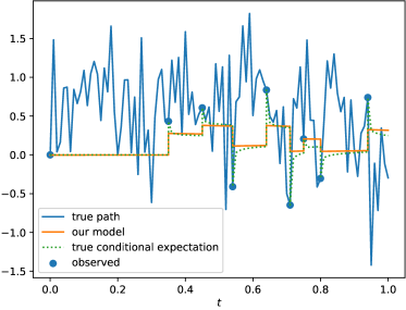
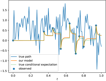
Figure 12: The same test sample of a fractional Brownian motion, when NJ-ODE (with signature) is trained with the original loss function (left) and the equivalent loss function (right). The equivalent loss function prevents NJ-ODE to end up in local minima.

D.2 Details for Poisson Point Process

Dataset. The easiest way to sample of a homogeneous Poisson point process is to use its property that interarrival times are i.i.d. exponential random variables with mean $1/\lambda$. Hence, for each path, we sample as many i.i.d. random variables $E_{k}\sim Exp(\lambda)$ as needed, such that $\sum_{k}E_{k}\geq T$. Then the cumulative sums $(\sum_{k\leq i}E_{k})_{i\geq 1}$ are the time points at which the process increases by $1$. In between it is constant and its starting point is $0$. Finally, the standard discretization time grid is applied to get one sample of the dataset.

Architecture. We use the standard NJ-ODE with the following architecture. The hidden size is $d_{H}=10$ and all 3 neural networks have the same structure of 2 hidden layers with $\tanh$ activation function and $50$ nodes.

D.3 Details for Uncertainty Estimation

Architecture. Since the dataset is relatively easy, we test a less complex network here to show that this can already be enough. In particular, we use the standard NJ-ODE with the following architecture. The hidden size is $d_{H}=50$, the readout network is a linear map and the other 2 neural networks have the same structure of 1 hidden layer with $\tanh$ activation function and $50$ nodes.

D.4 Details for Dependent Observation Intensity

Dataset. We use the Euler scheme to sample paths from a Black–Scholes model (geometric Brownian motion) with drift $\mu=2$, volatility $\sigma=0.3$, and starting value $X_{0}=1$.

Architecture. We use the PD-NJ-ODE with the following architecture. The latent dimension is $d_{H}=50$ and all 3 neural networks have the same structure of 2 hidden layers with $\tanh$ activation function and $50$ nodes. The signature is used up to truncation level $3$.

D.5 Details for Fractional Brownian Motion

Architecture. We compare the NJ-ODE, the NJ-ODE with signature, the NJ-ODE with recurrent jump network and the PD-NJ-ODE, all with the following architecture. The latent dimension is $d_{H}=50$ and all 3 neural networks have the same structure of 2 hidden layers with $\tanh$ activation function and $200$ nodes. All truncation levels $m\in\{1,\dotsc,10\}$ were tested and level $3$ gave the best trade-off between model performance and computation time. Therefore, results are only shown for only for truncation level $3$.

D.6 Details for Correlated 2-Dimensional Brownian Motion

Dataset. We use the same methods as described in Appendix D.1.3, but to account for the higher complexity of the dataset, we generate $100^{\prime}000$ samples instead of only $20^{\prime}000$.

Architecture. We use the PD-NJ-ODE with the following architecture. The latent dimension is $d_{H}=100$, the readout network is a linear map and the other 2 neural networks have the same structure of 1 hidden layer with $\tanh$ activation function and $100$ nodes. The signature is used up to truncation level $2$. This architecture achieves the minimal evaluation metric of $5.2\cdot 10^{-3}$. When changing to $\operatorname{ReLU}$ activation functions, this is nearly halved to $2.8\cdot 10^{-3}$.

D.7 Details for Stochastic Filtering

Dataset. We use the same methods as described in Appendix D.1.3, but to account for the higher complexity of the dataset, we generate $40^{\prime}000$ samples instead of only $20^{\prime}000$ and we generate training and testing datasets separately. In the training dataset, the $Y$-coordinates are observed at every observation time, while the $X$-coordinates are observed with probability $p_{k}=0.25$ (for each observation time a $Bernoulli(p_{k})$ random variable is drawn). In the test set, with $4^{\prime}000$ samples, the $Y$-coordinate is again observed at every observation time and the $X$-coordinate is never observed.

Architecture. We use the PD-NJ-ODE with the following architecture. The latent dimension is $d_{H}=200$ and all 3 neural networks have the same structure of $1$ hidden layer with $\tanh$ activation function and $100$ nodes. The signature is used up to truncation level $2$.

D.8 Details for Double Pendulum

Dataset. We use the same methods as described in Appendix D.1.3, but with $T=2.5$ and step size $0.025$, which leads again to $101$ time points. We chose a larger step size than usually, because the motion of the pendulums would otherwise be very slow, such that the resulting dataset would not seem very chaotic when sampling $100$ steps. However, it is important not to choose the step size too large, since otherwise the model is unable to see and learn the dynamics on a fine enough scale. To exemplify this, we generate a second dataset with $101$ time points, where $T=10$ and the step size is $0.1$. A comparison of the trained models on test samples of the two datasets is given in Figure 13, where we see that the model is not able to learn and reproduce more volatile parts of the longer trajectories that well.

Architecture. We use the PD-NJ-ODE, with the following architecture. The latent dimension is $d_{H}=400$ and all 3 neural networks have the same structure of $1$ hidden layers with $\tanh$ activation function and $200$ nodes. Empirically, the model performed best when using the recurrent jump network, but no signature terms as input.

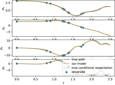
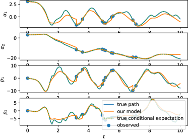
Figure 13: Predicted conditional expectation on test samples of the Double Pendulum dataset. Since the system is deterministic, the true conditional expectation coincides with the true path. Left: dataset with $T=2.5$. Right: dataset with $T=10$. Both using $100$ steps.

D.9 Details for Brownian Motion and its Time-Lagged Version

Dataset. We use the same methods as described in Appendix D.1.3, but we generate training and testing datasets separately. In both dataset, the $X$-coordinate is observed at every observation time $t_{i}$, and the $Y$-coordinate is observed at $t_{i}+\alpha$, where $\alpha=0.19$. In the test set, with $4^{\prime}000$ samples, the $Y$-coordinate is not observed at any additional time points. Only in the training dataset, the $Y$-coordinate is additionally observed with probability $0.5$ at any $t_{i}+\Delta t$, where $\Delta t$ is the used step size. We note that this is not general enough to satisfy the assumptions (cf. Section B.2). However, it suffices for the model to learn the correct behaviour and empirically leads to better results than using a dataset, where the $Y$-coordinate could be observed at all times between $t_{i}$ and $t_{i}+\alpha$. Indeed, the optimal evaluation metric on this dataset was $1.2\times 10^{-3}$.

Architecture. We use the PD-NJ-ODE with the following architecture. The latent dimension is $d_{H}=400$, the readout network is a linear map and the other 2 neural networks have the same structure of 1 hidden layer with $\operatorname{ReLU}$ activation function and $200$ nodes. The signature is used up to truncation level $2$.

D.10 Details for PhysioNet

Dataset. Details on the dataset are given in Herrera et al. (2021, Appendix F.5.3). The exact same setup is used.

Architecture. We use the PD-NJ-ODE with the following architecture. The hidden size is $d_{H}=50$, and all neural networks have the same structure of 1 hidden layer with $\tanh$ activation function and $50$ nodes. The signature is used up to truncation level $2$. Due to the exponential growth of the network size in the truncation level of the signature, no larger levels were tested.

Training. The training was done as specified in Section D.1.4, except that a batch size of $50$ was used for $175$ epochs. $5$ runs of the same network with random initializations were performed, over which the mean and standard deviation were computed.

Results. The minimal MSE on the test set during the $175$ epochs is reported. If instead reporting the MSE of the epoch where the training loss is minimal, the result is $1.957\pm 0.018(\times 10^{-3})$, also outperforming the results of NJ-ODE.

D.11 Details for Limit Order Book Dataset

Datasets. The widely used benchmark dataset for midprice forecasting (Ntakaris et al., 2018) is unfortunately not suitable in our context, since the time-stamps (or time differences between LOB updates) are not included in the dataset. Hence, the PD-NJ-ODE model could not be applied without adding some artificial time.
Therefore, we test our model on the crypto-currency LOB datasets “BTC”, “BTC1sec” and “ETH1sec” as described in Section 8.7. The datasets have $10^{\prime}297$ (“BTC”), $8^{\prime}669$ (“BTC1sec”) and $8^{\prime}753$ (“ETH1sec”) samples, which are split into the first $80\%$ as training and the last $20\%$ as testing data (such that no lookahead bias is introduced). While the “BTC” is based on the complete LOB of one day (July 2, 2020), the datasets “BTC1sec” and “ETH1sec” are based on snapshots at a frequency of 1 second of roughly 12 days (April 7-19, 2021). The median time step in the “BTC” dataset is approximately $0.025$, which means that on average $40$ updates of the order book happen every second. However, not every update affects the first $10$ levels of the order book in which we are interested. Overall, comparing the number of samples of the datasets, we can conclude that there are roughly $14$ updates to the first $10$ levels of the order book each second.
The labels (increase, decrease, stationary) for the classification task are computed as outlined in Zhang et al. (2019, Equation 4), where the threshold $\alpha$ is chosen to be the empirical $\frac{2}{3}$-quantile of the dataset, such that there is roughly the same number of samples for each label. Importantly, the labels are computed before any other preprocessing is applied to the data, which otherwise might lead to different labels.
For the DeepLOB model, the dataset is normalized by $z$-scores as it was done in Zhang et al. (2019). For the PD-NJ-ODE model, the dataset is not normalized, but each sample is shifted such that it starts at $X_{0}=0$ (for the DeepLOB this makes the performance worse, while not shifting for PD-NJ-ODE does not lead to a significant change of the performance). Moreover, the time is shifted such that each sample starts at $t_{0}=0$. Furthermore, we do not use the volume but only the midprice and the bid/ask prices up to level 10 as input for the PD-NJ-ODE.

Architecture. We use the PD-NJ-ODE with the following architecture. The hidden size is $d_{H}=100$, and all neural networks have the same structure of 1 hidden layer with $\tanh$ activation function and $50$ nodes. The signature is used up to truncation level $2$, but no recurrent jump network is used. On top of this architecture a classifier network, again with the same structure as the networks above, but with a final softmax activation (to produce outputs in $[0,1]$ that can be interpreted as probabilities), is used to map the last latent variable $H_{t_{n}}$ to the class probabilities $(p_{inc},p_{stat},p_{dec})\in[0,1]^{3}$. In the additional retraining of the classifier, we also test to use more complex classification networks, which lead to better results. In particular, in the results shown in Table 5, we retrained 3 different classifier networks with the architectures

• 1 hidden layer with $\tanh$ activation function and $50$ nodes (same as in combined training),

• 2 hidden layers with $\tanh$ activation functions and $200$ nodes,

• 4 hidden layers with $\tanh$ activation functions and $200$ nodes,

and reported the results of the best performing one, although all architectures achieved very similar results (less than $3\%$ deviation from reported F1-scores).

Training and Evaluation. The model is first trained for $50$ epochs, where the sum (without weighting) of the PD-NJ-ODE loss and the cross-entropy loss of the classifier is minimized with the standard Adam optimizer. The batch size is chosen to be $50$ and the learning rate is $0.01$. The model is trained to forecast all inputs, i.e., the midprice as well as all bid and ask prices up to level $10$, however, in the evaluation of the MSE only the midprice is considered.
The classifier is retrained for $1000$ epochs with the cross-entropy loss alone, also with the standard Adam optimizer. The batch size is again $50$ and the learning rate is $0.001$.

Training of baseline model DeepLOB. We use the training procedure that was suggested in Zhang et al. (2019). In particular, the model is trained with a batch size of $64$ for $50$ epochs and learning rate $0.0001$.

Additional Results

Appendix E Direct Neural Network Approximating of the Conditional Expectation

Revisiting the setting and our assumptions in Section 2, a question that might arise is, why we do not approximate the conditional expectation directly, by approximating the functions $F_{j}$ for $1\leq j\leq d_{X}$. The assumption that all functions $F_{j}$ are continuous is needed in any case, hence, using neural networks to approximate them should, in principle, be possible within this setting. Moreover, also in our used approach, we approximate the functions $F_{j}$ by the neural network $\rho$, however, only at observation times. From a theoretical point of view, the benefit of using this direct approximation clearly is that it works with weaker assumptions. In particular, continuity of $F_{j}$ instead of continuous differentiability of $F_{j}$ in its first coordinate $t$ would be enough.
In contrast to this, our approach makes use of additional domain knowledge, i.e., the fact that we can split up the learning problem into two intertwined sub-problems, where the one is to learn the continuous evolution between any two observation times and the other is to learn the updates (jumps) at observation times when new information becomes available. For the continuous learning part, we have the additional knowledge that this is the limit of a recursive problem, which amounts to learning the neural ODE network. In particular, instead of learning the function at every point in time, we only need to learn the dynamics that update the value of the function through time.

It turns out that making use of this domain knowledge, practically makes the learning task much easier. To quantify this, we compare the PD-NJ-ODE model to the approach of directly approximating $F_{j}$ by a neural network (which we refer to as NJ-model) on the simple Black–Scholes (geometric Brownian motion) dataset. While the PD-NJ-ODE achieves a minimal evaluation metric of $5\times 10^{-4}$ on the test set, the one of the NJ-model is $1\times 10^{-2}$, i.e., larger by a factor of $20$.

E.1 Implementation Details

Dataset. We use a Black–Scholes model with the parameters described in Section D.4 and sample the observation times as described in Section D.1.3.

Architecture. For the PD-NJ-ODE we use the following architecture. The latent dimension is $d_{H}=50$ and all 3 neural networks have the same structure of $1$ hidden layer with $\tanh$ activation function and $100$ nodes. The signature is used up to truncation level $2$. This architecture has approximately $27$K trainable parameters.
For the NJ-model we only use the neural network $\rho$ which directly maps to the output space, i.e., without a latent space and therefore also without a readout map. We first test using the same network as above, i.e., $1$ hidden layer with $\tanh$ activation function and $100$ nodes. When using the network structure as suggested by the functions $F_{j}$, i.e., without any recurrent structure and only with the signature as input, the minimal evaluation metric is $8\times 10^{-2}$. A recurrent structure, similar as in PD-NJ-ODE, which uses the output of the previous time as an input, improves this to $2\times 10^{-2}$. We remark that this network structure also uses some of the domain knowledge, however, in a way that the reduced assumptions are still sufficient. Since this model only has about $1$K trainable parameters, it might be considered unfair to compare it with the PD-NJ-ODE model above. Therefore, we test two larger architectures, first a network with $1$ hidden layer with $\tanh$ activation function and $2000$ nodes (resulting in $24$K trainable parameters) and secondly a network with $2$ hidden layers each with $\tanh$ activation function and $200$ nodes (resulting in $42$K trainable parameters). While the first architecture did not improve the results, the second one led to the reported evaluation metric of $1\times 10^{-2}$.

References

- Andersen & Piterbarg (2007) Leif BG Andersen and Vladimir V Piterbarg. Moment explosions in stochastic volatility models. Finance and Stochastics, 11(1):29–50, 2007.
- Andersson et al. (2023) William Andersson, Jakob Heiss, Florian Krach, and Josef Teichmann. Extending path-dependent NJ-ODEs to noisy observations and a dependent observation framework. arXiv, 2023.
- Bain & Crisan (2009) Alan Bain and Dan Crisan. Fundamentals of stochastic filtering, volume 3. Springer, 2009.
- Billingsley (1995) Patrick Billingsley. Probability and Measure. J. Wiley, third ed. edition, 1995.
- Bonnier et al. (2019) Patric Bonnier, Patrick Kidger, Imanol Perez Arribas, Cristopher Salvi, and Terry Lyons. Deep signature transforms. arXiv, 2019.
- Brouwer et al. (2019) Edward De Brouwer, Jaak Simm, Adam Arany, and Yves Moreau. GRU-ODE-Bayes: Continuous modeling of sporadically-observed time series. NeurIPS, 2019.
- Bugajewski & Gulgowski (2020) Dariusz Bugajewski and Jacek Gulgowski. On the characterization of compactness in the space of functions of bounded variation in the sense of Jordan. Journal of Mathematical Analysis and Applications, 484(2), 2020.
- Cao et al. (2018) Wei Cao, Dong Wang, Jian Li, Hao Zhou, Lei Li, and Yitan Li. Brits: Bidirectional recurrent imputation for time series. Advances in Neural Information Processing Systems, 31, 2018.
- Che et al. (2018) Zhengping Che, Sanjay Purushotham, Kyunghyun Cho, David Sontag, and Yan Liu. Recurrent neural networks for multivariate time series with missing values. Scientific Reports, 8, 2018.
- Chen et al. (2018) Ricky T. Q. Chen, Yulia Rubanova, Jesse Bettencourt, and David Duvenaud. Neural ordinary differential equations. NeurIPS, 2018.
- Chevyrev & Kormilitzin (2016) Ilya Chevyrev and Andrey Kormilitzin. A primer on the signature method in machine learning. arXiv, 2016.
- Cohen & Elliott (2015) Samuel N Cohen and Robert James Elliott. Stochastic calculus and applications. Springer, 2015.
- Debicki & Kisowski (2008) Krzysztof Debicki and Pawel Kisowski. A note on upper estimates for Pickands constants. Statistics & Probability Letters, 78(14):2046–2051, 2008.
- Dixon et al. (2017) Matthew Dixon, Diego Klabjan, and Jin Hoon Bang. Classification-based financial markets prediction using deep neural networks. Algorithmic Finance, 6(3-4):67–77, 2017.
- Durrett (2010) Rick Durrett. Probability: Theory and examples. New York, NY, USA, 4th edition, 2010.
- Eaton (2007) Morris L Eaton. Multivariate statistics: A vector space approach. Institute of Mathematical Statistics, 2007.
- Fermanian (2020) Adeline Fermanian. Embedding and learning with signatures, 2020.
- Goldberger et al. (2000) Ary L. Goldberger, Luis A. N. Amaral, Leon Glass, Jeffrey M. Hausdorff, Plamen Ch. Ivanov, Roger G. Mark, Joseph E. Mietus, George B. Moody, Chung-Kang Peng, and H. Eugene Stanley. Physiobank, physiotoolkit, and physionet. Circulation, 2000.
- Gubinelli (2016) Massimiliano Gubinelli. Stochastic analysis, course note 4, lecture notes, 2016. URL https://www.iam.uni-bonn.de/fileadmin/user_upload/gubinelli/stochastic-analysis-ss16/sa-note-4.pdf. Accessed: 2020-11-17.
- Hasselblatt & Katok (2003) Boris Hasselblatt and Anatole Katok. A first course in dynamics: With a panorama of recent developments. Cambridge University Press, 2003. doi: 10.1017/CBO9780511998188.
- Herrera et al. (2021) Calypso Herrera, Florian Krach, and Josef Teichmann. Neural jump ordinary differential equations: Consistent continuous-time prediction and filtering. In International Conference on Learning Representations, 2021.
- Hornik (1991) Kurt Hornik. Approximation capabilities of multilayer feedforward networks. Neural networks, 4(2):251–257, 1991.
- Hornik et al. (1989) Kurt Hornik, Maxwell Stinchcombe, and Halbert White. Multilayer feedforward networks are universal approximators. Neural Networks, 2, 1989.
- Jordan (1997) Michael I Jordan. Serial order: A parallel distributed processing approach. In Advances in Psychology, volume 121. Elsevier, 1997.
- Karandikar & Rao (2018) Rajeeva L. Karandikar and B. V. Rao. Introduction to Stochastic Calculus. Indian Statistical Institute Series. Springer Singapore, Singapore, 2018. ISBN 978-981-10-8317-4. doi: 10.1007/978-981-10-8318-1. URL http://link.springer.com/10.1007/978-981-10-8318-1.
- Keller-Ressel (2011) Martin Keller-Ressel. Moment explosions and long-term behavior of affine stochastic volatility models. Mathematical Finance: An International Journal of Mathematics, Statistics and Financial Economics, 21(1):73–98, 2011.
- Kidger et al. (2020) Patrick Kidger, James Morrill, James Foster, and Terry Lyons. Neural controlled differential equations for irregular time series. Advances in Neural Information Processing Systems, 33, 2020.
- Kidger et al. (2021) Patrick Kidger, James Foster, Xuechen Li, and Terry J Lyons. Neural SDEs as infinite-dimensional GANs. In International conference on machine learning, pp. 5453–5463. PMLR, 2021.
- Kiraly & Oberhauser (2019) Franz J. Kiraly and Harald Oberhauser. Kernels for sequentially ordered data. Journal of Machine Learning Research, 20(31):1–45, 2019.
- Lapeyre & Lelong (2021) Bernard Lapeyre and Jérôme Lelong. Neural network regression for Bermudan option pricing. Monte Carlo Methods and Applications, 27(3):227–247, 2021.
- Ledoux & Talagrand (1991) Michel Ledoux and Michel Talagrand. Probability in banach spaces. Springer-Verlag, 62, 1991.
- Li et al. (2020) Xuechen Li, Ting-Kam Leonard Wong, Ricky TQ Chen, and David K Duvenaud. Scalable gradients and variational inference for stochastic differential equations. In Symposium on Advances in Approximate Bayesian Inference, pp. 1–28. PMLR, 2020.
- Morrill et al. (2021) James Morrill, Cristopher Salvi, Patrick Kidger, and James Foster. Neural rough differential equations for long time series. In International Conference on Machine Learning, pp. 7829–7838. PMLR, 2021.
- Morrill et al. (2022) James Morrill, Patrick Kidger, Lingyi Yang, and Terry Lyons. On the choice of interpolation scheme for neural CDEs. Transactions on Machine Learning Research, 2022. ISSN 2835-8856.
- Nielsen (2021) Martin Sogaard Nielsen. High frequency crypto limit order book data, 2021. URL https://www.kaggle.com/datasets/martinsn/high-frequency-crypto-limit-order-book-data. Accessed: 2023-09-21.
- Norros et al. (1999) Ilkka Norros, Esko Valkeila, and Jorma Virtamo. An elementary approach to a Girsanov formula and other analytical results on fractional Brownian motions. Bernoulli, 5(4):571 – 587, 1999.
- Ntakaris et al. (2018) Adamantios Ntakaris, Martin Magris, Juho Kanniainen, Moncef Gabbouj, and Alexandros Iosifidis. Benchmark dataset for mid-price forecasting of limit order book data with machine learning methods. Journal of Forecasting, 37(8):852–866, 2018.
- Passalis et al. (2018) Nikolaos Passalis, Anastasios Tefas, Juho Kanniainen, Moncef Gabbouj, and Alexandros Iosifidis. Temporal bag-of-features learning for predicting mid price movements using high frequency limit order book data. IEEE Transactions on Emerging Topics in Computational Intelligence, 4(6):774–785, 2018.
- Protter (2005) Philip Protter. Stochastic integration and differential equations. Springer-Verlag, 2005.
- Reizenstein & Graham (2018) Jeremy Reizenstein and Benjamin Graham. The iisignature library: Efficient calculation of iterated-integral signatures and log signatures. arXiv, 2018.
- Rubanova et al. (2019) Yulia Rubanova, Ricky T. Q. Chen, and David K Duvenaud. Latent ordinary differential equations for irregularly-sampled time series. NeurIPS, 2019.
- Rubinstein & Shapiro (1993) Reuven Y Rubinstein and Alexander Shapiro. Discrete event systems: Sensitivity analysis and stochastic optimization by the score function method. Wiley, 1993.
- Rumelhart et al. (1985) David E Rumelhart, Geoffrey E Hinton, and Ronald J Williams. Learning internal representations by error propagation. Technical report, California Univ San Diego La Jolla Inst for Cognitive Science, 1985.
- Saxena & Cao (2021) Divya Saxena and Jiannong Cao. Generative adversarial networks (GANs) challenges, solutions, and future directions. ACM Computing Surveys (CSUR), 54(3):1–42, 2021.
- Shao (1996) Qi-Man Shao. Bounds and estimators of a basic constant in extreme value theory of Gaussian processes. Statistica Sinica, 6(1):245–257, 1996.
- Sottinen & Viitasaari (2017) Tommi Sottinen and Lauri Viitasaari. Prediction law of fractional Brownian motion. arXiv, 2017.
- Svirin (2009) Alex Svirin. Double pendulum, 2009. URL https://math24.net/double-pendulum.html. Accessed: 2022-09-23.
- Taraldsen (2018) Gunnar Taraldsen. Optimal learning from the Doob-Dynkin lemma. arXiv, 2018.
- Tran et al. (2017) Dat Thanh Tran, Martin Magris, Juho Kanniainen, Moncef Gabbouj, and Alexandros Iosifidis. Tensor representation in high-frequency financial data for price change prediction. In 2017 IEEE Symposium Series on Computational Intelligence (SSCI), pp. 1–7. IEEE, 2017.
- Tsantekidis et al. (2017) Avraam Tsantekidis, Nikolaos Passalis, Anastasios Tefas, Juho Kanniainen, Moncef Gabbouj, and Alexandros Iosifidis. Forecasting stock prices from the limit order book using convolutional neural networks. In 2017 IEEE 19th conference on business informatics (CBI), volume 1, pp. 7–12. IEEE, 2017.
- Tsantekidis et al. (2020) Avraam Tsantekidis, Nikolaos Passalis, Anastasios Tefas, Juho Kanniainen, Moncef Gabbouj, and Alexandros Iosifidis. Using deep learning for price prediction by exploiting stationary limit order book features. Applied Soft Computing, 93:106401, 2020.
- Tzen & Raginsky (2019) Belinda Tzen and Maxim Raginsky. Neural stochastic differential equations: Deep latent Gaussian models in the diffusion limit. arXiv, 2019.
- Zhang et al. (2019) Zihao Zhang, Stefan Zohren, and Stephen Roberts. Deeplob: Deep convolutional neural networks for limit order books. IEEE Transactions on Signal Processing, 67(11):3001–3012, 2019.