On validity of different PDFs sets using the proton $k_{t}$-factorization structure functions and the Gaussian $k_{t}$-dependence of KMR UPDFs

Abstract

In this work, we discuss: (i) The ratios of different parton distribution functions (PDFs), i.e., MMHT2014, CJ15, CTEQ6l1, HERAPDF15, MSTW2008, HERAPDF20 and MSHT20, and the corresponding Kimber-Martin-Ryskin (KMR) unintegrated parton distribution functions (UPDFs) sets versus the hard scale $Q^{2}$, to find out the sensibility of the KMR UPDFs with respect to the input PDFs sets. It is shown that there is not much difference between the different input-PDFs or corresponding UPDFs sets ratios. (ii) Then, the dependence of proton $k_{t}$-factorization structure functions on the different UPDFs sets which can use the above PDFs sets as input, are presented. The results are compared with the experimental data of ZEUS, NMC and H1+ZEUS at the hard scale $Q^{2}=27$ and $90$ $GeV^{2}$, and a reasonable agreement is found, considering different input PDFs sets. (iii) Furthermore, by fitting a Gaussian function, which depends on the transverse momentum $k_{t}$, to the KMR UPDFs and averaging over $x$ (the fractional parton momentum), we obtain the average transverse momentum, $<k_{t}^{2}>$, in the scale range $Q^{2}=2.4-1.44\times 10^{4}$ $GeV^{2}$, which is in agreement with the other groups predictions, $0.25-0.44$ $GeV^{2}$ at $Q^{2}=2.4$ $GeV^{2}$. (iv) Finally we explore the average transverse momentum for which, the results of proton structure function with the KMR UPDFs and that of the Gaussian $k_{t}$-dependent, are consistent to each other. Through the above report, at each step the parton branching (PB) UPDFs, i.e., the transverse momentum dependent PDFs (PB TMDPDFs) are considered for comparisons with the corresponding KMR UPDFs output.

I Introduction

Understanding of the proton structure function (SF) is crucial for obtaining an accurate description of the proton-proton collisions experimental data for example at the LHC ATLAS ; LHC ; CMS2021 . The parton distribution functions (PDFs) ATLAS ; LHC ; CMS2021 , are the main elements in understanding of the structure of hadrons and also are essential ingredients in the phenomenological calculations of high energy physics experiments. The PDFs are mostly obtained by the global analysis of hard scattering data in the collinear factorization framework. Within this framework, the PDFs ($a(x,\mu^{2})$, $a=g,q$ and $\bar{q}$) depend on $x$, the longitudinal momentum fraction of the partons with respect to proton, and $\mu^{2}=Q^{2}$, the hard scale. In the collinear factorization it is assumed that partons have negligible transverse momentum, i.e., $k_{t}^{2}\ll\mu^{2}$, and the PDFs follow the Dokshitzer–Gribov–Lipatov–Altarelli–Parisi (DGLAP) DGLAP1 ; DGLAP2 ; DGLAP3 ; DGLAP4 evolution equation. However, the parton transverse momentum becomes important at the high energy limit, where $x$ is small, and therefore it is needed to have the transverse momentum dependent (TMD) PDFs (TMDPDFs), or unintegrated parton distribution functions (UPDFs) CMS2021 , which are based on the DGLAP DGLAP1 ; DGLAP2 ; DGLAP3 ; DGLAP4 and Balitskii-Fadin-Kuraev-Lipatov (BFKL) BFKL1 ; BFKL2 ; BFKL3 equations.

The UPDFs ($f_{a}(x,k_{t}^{2},\mu^{2})$) depend on the transverse momentum $k_{t}$ of parton, besides having dependency on $x$ and $\mu^{2}$, and are historically defined for gluon which satisfies the Catani–Ciafaloni-Fiorani–Marchesini (CCFM) ccfm1 ; ccfm2 ; ccfm3 ; ccfm4 evolution equation. However, in order to obtain the quark UPDFs one needs to use other methods such as Kimber-Martin-Ryskin (KMR) KMR ; KMR1 or Martin-Ryskin-Watt (MRW) MRW or parton branching (PB) PB1 ; PB2 ; PBTMD approaches.

The general behavior and stability of the KMR and MRW models are investigated in details in the references Modarres1 ; Modarres2 ; Modarres3 ; Modarres4 , where these two models show promising results in describing the experimental data Modarres5 ; Modarres6 ; Modarres7 ; Modarres8 ; Modarres9 . As we mentioned above, the KMR and MRW formalisms are based on the DGLAP and BFKL evolution equations, as well as the Sudakov form factor, and the collinear PDFs as their input. They become scale ($\mu^{2}$) dependent only at the last evolution step. The ambiguity about the differential forms of KMR and MRW is discussed in the reference kordp

The KMR and MRW frameworks are generally different from each other by the various imposition of angular ordering constraints and this leads to relatively small different behavior of these models in the phenomenological studies. Also because the collinear input PDFs play an important role in these UPDFs models, therefore the investigation of various PDFs sets are vital in any phenomenological analysis. Here, in this work for investigation of their dependency to the PDFs sets, in the $k_{t}$-factorization framework, we only consider the KMR model where in the references Modarres2014 ; Modarres2019 it is shown that KMR model UPDFs performs better than the MRW one, in describing the deep inelastic proton structure functions, $F_{2}(x,Q^{2})$. In contrast to the KMR and MRW models, within the PB model it is claimed that, the transverse momentum dependency comes into play from the start of the evolution ladder to obtain the UPDFs global analysis. This model also shows promising results in describing the experimental data PB_Drell ; Modarres8 ; PBTMD . As a result of having different methods for obtaining the UPDFs, therefore it is important to test these different approaches against the experimental data to gain a better insight of their behaviors and performances in various energy limits, i.e., $\mu^{2}$, especially in the $k_{t}$ factorization framework.

In addition to the aforementioned UPDFs models described above, it is also conventional to consider Gaussian distribution for the $k_{t}$ dependency of UPDFs. For example in calculating the cross section of the semi-inclusive deep-inelastic-scattering (SIDIS) processes, the unintegrated fragmentation functions (UFFs) Metz ; Signori ; Miguel ; Anselmino1 ; Anselmino2 ; Schweitzer ; T1 , and also the UPDFs with the Gaussian distribution are considered, where for the UPDFs, it is usually written as below:

$$f_{a}(x,k_{t}^{2},\mu^{2})=f_{a}(x,\mu^{2}){e^{-{k_{t}^{2}\over<k_{t}^{2}>}}\over\pi<k_{t}^{2}>}.$$ (1)

It should be mentioned that, these distributions can also describe the data at small scales limit, and the cross section calculations with these Gaussian distributions can cover the data well T2 . Therefore, it is interesting to investigate this distribution at larger scales and also examine the dependency of the average transverse momentum $<k_{t}^{2}>$ by changing the hard scale $\mu^{2}$ and the $x$ value for the UPDFs.

The purpose of the present work is to investigate the sensitivity of KMR UPDFs to the various input sets of PDFs. For this reason, after obtaining the ratio of different sets of PDFs and UPDFs, we calculate the proton $k_{t}$ factorization structure function for these UPDFs sets to find out which PDFs (UPDFs) sets give the closer results regarding the available experimental data, i.e., NMC (NMC, ), ZEUS (ZEUS, ) and H1+ZEUS (H1+ZEUS, ). The SF with the PB TMDPDFs PB1 ; PB2 ; PB_Drell ; PBTMD are also calculated and the PB TMDPDFs ratios to the KMR UPDFs are discussed, as well.

Therefore, the structure of the paper is arranged as follows: In the subsections II.1 and II.2, we present the KMR UPDFs method and the calculation of PB TMDPDFs, as well as the proton $k_{t}$-factorization structure function, respectively. The ratio of UPDFs using various PDFs sets for different values of $x$ and transverse momentum $k_{t}$, and the results of fitting the Gaussian function to the KMR UPDFs are given in the subsections III.1 and III.2, respectively. We also plot the variation of average transverse momentum versus the $x$ values for the two different energy scales. The results of proton structure functions for different UPDFs models, i.e., the KMR, PB and Gaussian transverse momentum dependent UPDFs models are given in the subsection III.3. Finally, in the section IV our conclusions will be presented.

II The general formalisms for the KMR UPDFs and the PB TMDPDFs calculation and the proton $k_{t}$-factorization structure functions

II.1 The UPDFs of KMR method and the PB TMDPDFs

The KMR UPDFs, $f_{a}(x,k_{t}^{2},\mu^{2})$, can be calculated through the KMR (KMR, ; KMR1, ) procedure, based on the DGLAP and BFKL approaches. The inputs are the single-scale PDFs, i.e., $a(x,\mu^{2})=xq(x,\mu^{2}),x\bar{q}(x,\mu^{2}),xg(x,\mu^{2})$, and the leading order (LO) splitting functions $P_{aa^{\prime}}(x)$. The modified DGLAP equations is usually written as (KMR, ; KMR1, ),

$$\frac{\partial a(x,\mu^{2})}{\partial\ln\mu^{2}}=\frac{\alpha_{s}}{2\pi}\left[\int_{x}^{1-\Delta}dzP_{aa^{\prime}}(z)a^{\prime}(\frac{x}{z},\mu^{2})-a(x,\mu^{2})\sum_{a^{\prime}}\int_{0}^{1-\Delta}P_{a^{\prime}a}(z^{\prime})dz^{\prime}\right],$$ (2)

where the cut-off $\Delta$, prevents the $z=1$ singularities in $P_{aa^{\prime}}(x)$ arises from the soft gluon emission (note that for $g\rightarrow gg$ splitting, an extra factor $z^{\prime}$ should be inserted in the front of $P_{aa^{\prime}}$ in the last integral of equation (2)). The cutoff $\Delta$ can be obtained from the well known angular ordering condition (ccfm1, ; ccfm2, ; ccfm3, ; QCD, ; Kimber, ), in the last evolution step, so,

$$\Theta(\theta-\theta^{\prime})\Rightarrow\mu>\frac{zk_{t}}{1-z},$$ (3)

which leads to an upper limit on the integration variable $z$, i.e.,

$$z_{max}=\frac{\mu}{\mu+k_{t}}\Rightarrow\Delta=1-z_{max}=\frac{k_{t}}{\mu+k_{t}}$$ (4)

The re-summation of all virtual contributions, i.e., the second term of the equation (2), leads to the survival probability Sudakov form factor as,

$$T_{a}(k_{t},\mu)=exp\left(-\int_{k_{t}^{2}}^{\mu^{2}}{\alpha_{S}(k^{\prime 2}_{t})\over 2\pi}\frac{dk^{\prime 2}_{t}}{k^{\prime 2}_{t}}\sum_{a^{\prime}}\int^{1-\Delta}_{0}dz^{\prime}P_{a^{\prime}a}(z^{\prime})\right).$$ (5)

Finally the explicit form of the KMR UPDFs can be written as follows:
(i) for the quarks and the anti-quarks ($q^{\prime}=q,\bar{q}$),

$$f_{q^{\prime}}(x,k_{t}^{2},\mu^{2})=T_{q^{\prime}}(k_{t},\mu){\alpha_{S}(k_{t}^{2})\over 2\pi}\int^{1-\Delta}_{x}dz\left[P_{q^{\prime}q^{\prime}}(z){x\over z}q^{\prime}\left({x\over z},k_{t}^{2}\right)+P_{q^{\prime}g}(z){x\over z}g\left({x\over z},k_{t}^{2}\right)\right],$$ (6)

(ii) for the gluon:

$$f_{g}(x,k_{t}^{2},\mu^{2})=T_{g}(k_{t},\mu){\alpha_{S}(k_{t}^{2})\over 2\pi}\int^{1-\Delta}_{x}dz\left[\sum_{q^{\prime}=q,\bar{q}}P_{gq^{\prime}}(z){x\over z}q^{\prime}\left({x\over z},k_{t}^{2}\right)+P_{gg}(z){x\over z}g\left({x\over z},k_{t}^{2}\right)\right].$$ (7)

The dependence of KMR UPDFs, $f_{a}(x,k_{t}^{2},\mu^{2})$, on the two scales $k_{t}^{2}$ and $\mu^{2}$, are imposed on the last step evolution and the angular ordering is considered. The KMR formalism allows us to extend smoothly, the $k_{t}$ dependency of UPDFs into the region where $k_{t}>\mu$.

For the PB TMDPDFs PB_Drell ; PBTMD we use the TMDLIB given in the reference PBLINK , which can generate the PB TMDPDFs at various $x$ values, the hard scales, $\mu^{2}$, and the transverse momentum, $k_{t}$. One should note that the generated PB TMDPDFs through the TMDLIB are divided by $k_{t}^{2}$ with respect to the KMR UPDFs explained above.

II.2 The proton $k_{t}$-factorization Structure Function

In the deep-inelastic scattering of electron-proton, the gluon can only interact with the virtual photon through the intermediate quark or anti-quark by considering the electromagnetic interaction. Therefore three LO diagrams contribute to the calculation of structure function $F_{2}(x,Q^{2})$. The two of these diagrams are related to $g\rightarrow q\bar{q}$ which are shown as the box and the cross-box in the references (KMR, ; KMR1, ; Modarres2014, ; Modarres2019, ).

For calculation of the gluon contribution to the proton SF generated from the box and cross-box diagrams (using an angular average value $<\phi>=\frac{\pi}{4}$ KMR ; KMR1 ), we have:

$$F_{T}^{gluon\rightarrow quark}(x,Q^{2}) =\Sigma_{q=u,d,s,c}e_{q}^{2}\frac{Q^{2}}{4\pi}\int_{k_{0}^{2}}^{k_{max}^{2}}\frac{dk_{t}^{2}}{k_{t}^{4}}\int_{0}^{1}d\beta\int_{k_{0}^{2}}^{k_{max}^{2}}d\kappa_{t}^{2}\alpha_{s}(\mu^{2})$$ (8)

$$f_{g}(\frac{x}{\bar{z}},k_{t}^{2},\mu^{2})\Theta(1-\frac{x}{\bar{z}})\left(\left[\beta^{2}+(1-\beta)^{2}\right](J_{1}+J_{2}-J_{3})+m_{q}^{2}(J_{4}+J_{5}-J_{6})\right),$$

and

$$F_{L}^{gluon\rightarrow quark}(x,Q^{2}) =\Sigma_{q=u,d,s,c}e_{q}^{2}\frac{Q^{2}}{4\pi}\int_{k_{0}^{2}}^{k_{max}^{2}}\frac{dk_{t}^{2}}{k_{t}^{4}}\int_{0}^{1}d\beta\int_{k_{0}^{2}}^{k_{max}^{2}}d\kappa_{t}^{2}\alpha_{s}(\mu^{2})$$ (9)

$$f_{g}(\frac{x}{\bar{z}},k_{t}^{2},\mu^{2})\Theta(1-\frac{x}{\bar{z}})\left(4Q^{2}\beta^{2}(1-\beta)^{2})(J_{4}+J_{5}-J_{6})\right),$$

where $k_{max}=4Q$, $J$s are defined in the appendix A and,

$${1\over\bar{z}}=1+\frac{\kappa_{t}^{2}+m_{q}^{2}}{(1-\beta)Q^{2}}+\frac{\kappa_{t}^{2}+k_{t}^{2}-2k_{t}\kappa_{t}\cos<\phi>+m_{q}^{2}}{\beta Q^{2}}.$$ (10)

For the SF calculation of the non-perturbative part ($k_{t}<k_{0}$, $k_{0}=1$ $GeV$), we use:

$$\int_{0}^{k_{0}^{2}}\frac{dk_{t}^{2}}{k_{t}^{2}}f_{g}(x,k_{t}^{2},\mu^{2})[\frac{Remainder}{k_{t}^{2}}]=xg(x,k_{0}^{2})T_{g}(k_{0},\mu)\left[\right]_{k_{t}=a},$$ (11)

where $a$ is a number between $0$ and $k_{0}$ . $\beta$, similar to $x$, is a fraction of the photon momentum which is carried by the intermediate quark and $z$ is the fraction of gluon momentum that is transferred to the quark. If $x$ is the fraction of the proton momentum carried by the quark, then, the fraction of the proton momentum carried by gluon is equal to $\frac{x}{z}$. $k_{t}$ is the parent gluon transverse momentum and $\kappa_{t}$ is transverse momentum of daughter quark. We ignore the mass of light quarks and take the mass of charm quark to be equal to $m_{c}=1.4$ GeV and set,

$$\mu^{2}=k_{t}^{2}+\kappa_{t}^{2}+m_{q}^{2}.$$ (12)

The gluon contribution to the proton SF is equal to sum of the equations (8), (9) and (11).

For the SF of the process that the quark radiates gluon before interaction with the photon, the perturbative part of the quark contribution is:

$$F_{2}^{quarrk\rightarrow quark}(x,Q^{2})=\Sigma_{q=u,d,s,c}e_{q}^{2} \int_{k_{0}^{2}}^{Q^{2}}\frac{d\kappa_{t}^{2}}{\kappa_{t}^{2}}\frac{\alpha_{s}(\kappa_{t}^{2})}{2\pi}\int_{k_{0}^{2}}^{\kappa_{t}^{2}}\frac{dk_{t}^{2}}{k_{t}^{2}}\int_{x}^{Q/(Q+k_{t})}dz$$ (13)

$$\left[f_{q}(\frac{x}{z},k_{t}^{2},Q^{2})+f_{\bar{q}}(\frac{x}{z},k_{t}^{2},Q^{2})\right]p_{qq}(z).$$

While, for the non-perturbative region, the quark part of SF is related to the state in which a quark with a distribution function $xq(x,k_{0}^{2})$ enters the evolution chain from the non-perturbative region and interacts with the virtual photon without real radiation, i.e.,

$$F_{2}^{quark\rightarrow quark}(x,Q^{2})=\Sigma_{q=u,d,s,c}e_{q}^{2}\left[xq(x,k_{0}^{2})+x\bar{q}(x,k_{0}^{2})\right]T_{q}(k_{0},Q).$$ (14)

Then the quark contribution to the SF is sum of the equations (13) and (14).

Finally, the total proton SF ($F_{2}(x,Q^{2})$) becomes equal to sum of the quarks and gluon contributions, i.e., the equations (8), (9), (11), (13) and (14).

III Results and discussions

III.1 The PDFs of different groups data fitting sets ratios and their corresponding KMR UPDFs ratios

In this section the different groups data fittings PDFs sets such as: MMHT2014 (MMHT, ), CJ15 (CJ, ), CTEQ6l1 (cteq, ), HERAPDF15 (hera, ), MSTW2008 (mstw, ), MSHT20 (msht, ) and HERAPDF20 heranlo , at different $x$ values, which are generated through the LHAPDF6 library (LHAPDF, ) are investigated by calculating their up-quark PDFs ratios with respect to the MMHT2014 PDFs sets, see the figure 1. We chose MMHT2014 PDFs set because in our previous works it fits reasonably the SIDIS data Modarres2019 . There is a good agreement between the different groups PDFs sets especially above $10$ $GeV^{2}$. Only the HERAPDF20 PDFs set shows some deviations in the whole $Q^{2}$ region.

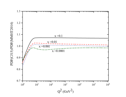
(a)

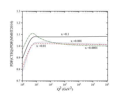
(b)

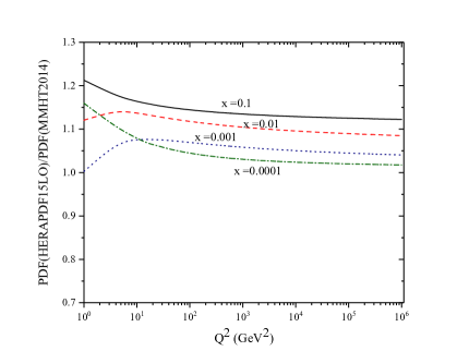
(c)

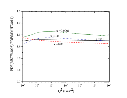
(d)

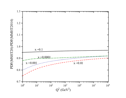
(e)

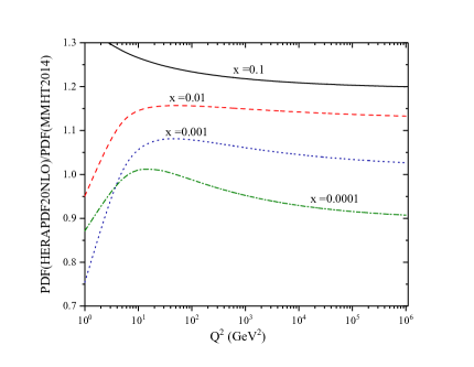
(f)

Figure 1: The different up-quark PDFs ratios for various $x$ values given in the panels (a), (b), (c), (d), (e) and (f).

In order to see the effect of KMR UPDFs (by using the KMR method presented in the subsection II.1) with various inputs PDFs sets, in the figures 2 and 3 the obtained up-quark UPDFs ratios with respect to the KMR UPDF(MMHT2014) for the longitudinal momentum fraction ${x=10^{-1},10^{-2},10^{-3},10^{-4}}$ and the transverse momentum $k_{t}^{2}=25$ and $10^{4}$ $GeV^{2}$ are plotted in terms of the hard scale $Q^{2}$.

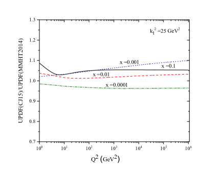
(a)

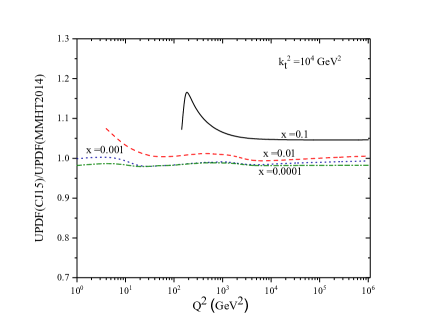
(b)

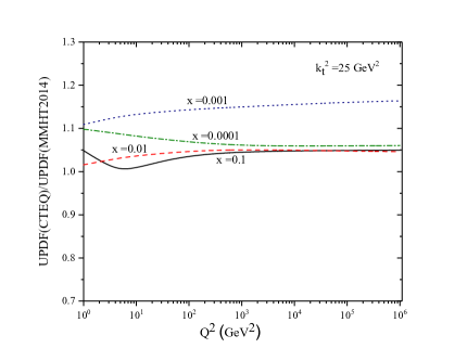
(c)

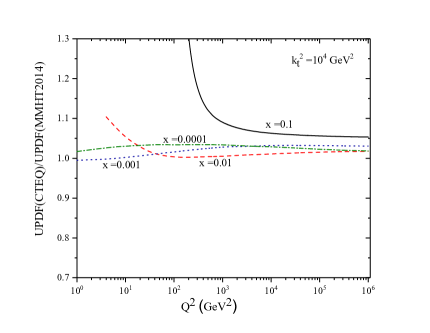
(d)

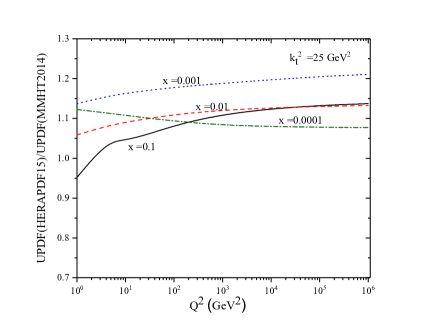
(e)

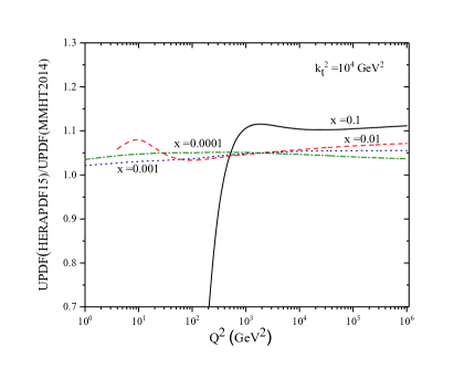
(f)

Figure 2: The different up quark UPDFs ratios of various groups PDFs sets with respect to MMHT2014 one, at the two $k_{t}^{2}$ and four $x$ values: The panels (a), (b), (c), (d), (e) and (f) .

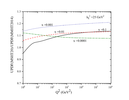
(a)

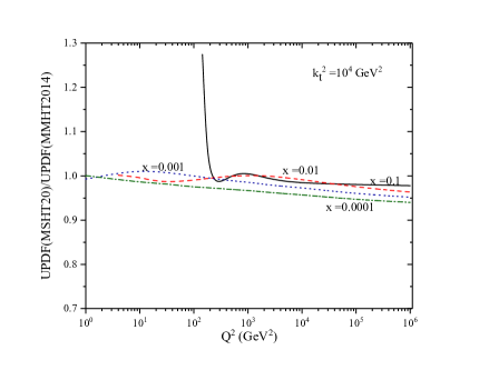
(b)

(c)

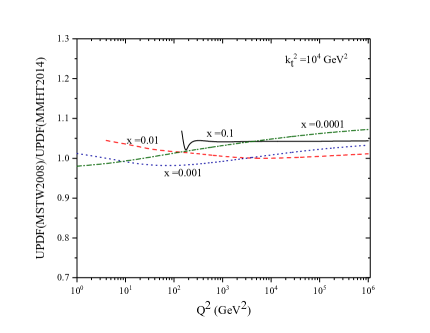
(d)

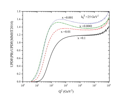
(e)

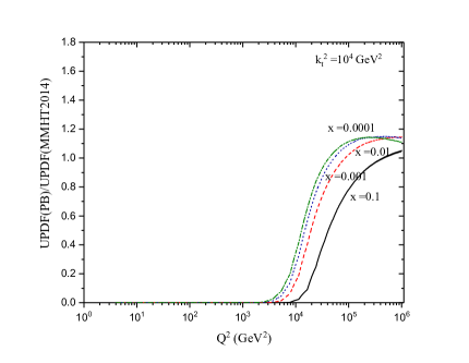
(f)

Figure 3: The different up quark UPDFs ratios of various groups PDFs sets with respect to MMHT2014 one, at the two $k_{t}^{2}$ and the four $x$ values: The panels (a), (b), (c), (d), (e) and (f).

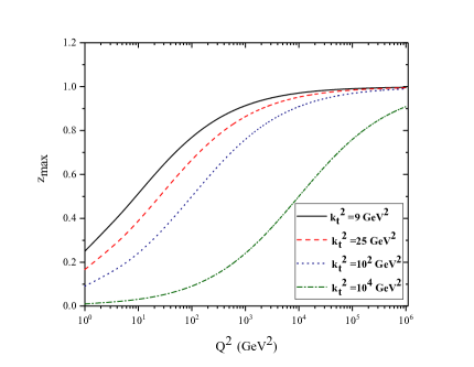
Figure 4: The $z_{max}$ versus the hard scale $Q^{2}$ Modarres1 . See the text for more explanations.

For all $x$ values a good agreement is observed between the different groups input PDFs sets, i.e., UPDFs, especially at large scale, which is rooted in the behavior of PDFs sets in the large hard scales. We should mention here that the Sudakov form factors are independent of the input PDFs sets, therefore, in the UPDFs ratios they are canceled out. On the other hand, the parton distributions of quarks and gluon in the equations (6) and (7) (in the form $xq(\frac{x}{z},k_{t}^{2})$, $x\bar{q}(\frac{x}{z},k_{t}^{2})$ and $xg(\frac{x}{z},k_{t}^{2})$) enter the calculations at the scale $\mu^{2}=k_{t}^{2}$. This causes the divergent behavior of different PDFs sets in the small scale (Modarres1, ) which affect the functional forms of UPDFs in the small $k_{t}^{2}$. Therefore, the result is an increase in the disagreement of the UPDFs with a decrease in $k_{t}^{2}$. In addition, the steeper and divergent in the UPDFs ratios appear in the larger $x$ values, which show themselves with increasing $k_{t}^{2}$ and move to larger $Q^{2}$. This divergence is rooted in the definition of $z_{max}$ (see the figure 4 Modarres1 ). In fact, this divergence occurs in the regions where the upper and lower limits of the integral are close to each other ($x\simeq z_{max}$) and depending on each UDPFs, tends to zero rapidly. So the ratio of UPDFs becomes zero or infinite. According to definition of $z_{max}=1-\Delta={Q\over(Q+k_{t})}$, the value of $Q$ around which this divergence occurs can be obtained for fixed $x$ and $k_{t}$, which is similar to the results of reference (Modarres1, ).

One can observe from the panels (e) and (f) of the figure 3 that the ratio of PB TMDPDFs to the corresponding UPDFs using MMHT2014 PDFs set, has different behaviors with respect to the other ratios in the panels of figures 2 and 3. This shows that the PB TMDPDFs are calculated with different and stronger constraint and cut-off with respect to that of KMR formalism. For example, since PB TMDPDFs become approximately zero for $Q^{2}<k_{t}^{2}$, the ratios go to zero in this range, but for $Q^{2}>k_{t}^{2}$ they become larger with respect to other panels ratios. This behavior roots to the normalization condition of the equation (16) (see the comments above this equation about the $k_{t}^{2}$ factor) and different constraint which imposed on the PB TMDPDFs. On the other hand, it uses HERAPDF20 PDFs which behave differently regarding the other PDFs sets.

III.2 The Gaussian transverse momentum dependent fit to the KMR UPDFS

As we pointed out in the introduction, the $k_{t}^{2}$ dependence of UPDFs, both in the perturbative and non-perturbative regions are usually assumed to have Gaussian shape PBTMD ; Metz ; Bacchetta ; T1 ; T2 with Gaussian width around $<k_{t}^{2}>=0.25-0.44$ $GeV^{2}$, at the hard scale equal to $2.4$ $GeV^{2}$. So it would be interesting to find out if the KMR UPDFs to have similar behavior. To calculate the average transverse momentum $<k_{t}^{2}>$, we plot the UPDFs using the KMR method for a constant scale $Q^{2}$ and $0.0045<x<0.1$, by using MSHT20 PDFs set in the LO approximation. The functional form that we fit to the UPDFs is as following (note that we multiply the Gaussian function by $k_{t}^{2}$ and omit the $\pi$ in the denominator of the equation (1), because of our definitions of UPDFs and the integration, i.e., $dk_{t}^{2}$ rather than $d^{2}k_{t}$) :

$$f_{a}(x,k_{t}^{2},\mu^{2})=f_{a}(x,\mu^{2}){k_{t}^{2}\over<k_{t}^{2}>}exp\left(-{k_{t}^{2}\over<k_{t}^{2}>}\right).$$ (15)

Then the normalization condition in the KMR method, i.e.,:

$$\int_{0}^{\mu^{2}}{dk_{t}^{2}\over k_{t}^{2}}f_{a}(x,k_{t}^{2},\mu^{2})=f_{a}(x,\mu^{2}),$$ (16)

is easily satisfied (where $f_{a}(x,\mu^{2})$ are the different PDFs sets). So, the Gaussian widths $<k_{t}^{2}>$ can be obtained for different $x$ values by fitting and averaging between them, are presented as the average transverse momentum $<k_{t}^{2}>$ at each scale $Q^{2}$.

Table 1: The values of average transverse momentum for the light quarks and gluon in the hard scales $Q^{2}=2.4$ to $1.44\times 10^{4}$ $GeV^{2}$.

$Q^{2}\;(GeV^{2})$	$<k_{t}^{2}>_{u}\;(GeV^{2})$	$<k_{t}^{2}>_{d}\;(GeV^{2})$	$<k_{t}^{2}>_{s}\;(GeV^{2})$	$<k_{t}^{2}>_{g}\;(GeV^{2})$
2.4	0.33	0.32	0.32	0.41
9	0.40	0.38	0.39	0.5
25	0.46	0.44	0.45	0.57
49	0.5	0.48	0.48	0.62
81	0.53	0.50	0.51	0.66
100	0.54	0.51	0.53	0.68
400	0.63	0.60	0.61	0.79
900	0.69	0.65	0.67	0.86
1600	0.73	0.7	0.72	0.92
2500	0.76	0.73	0.75	0.97
3600	0.79	0.76	0.78	1.01
4900	0.82	0.79	0.81	1.05
6400	0.84	0.81	0.83	1.10
8100	0.87	0.83	0.85	1.12
10000	0.89	0.85	0.87	1.15
12100	0.90	0.87	0.89	1.18
14400	0.92	0.88	0.91	1.21

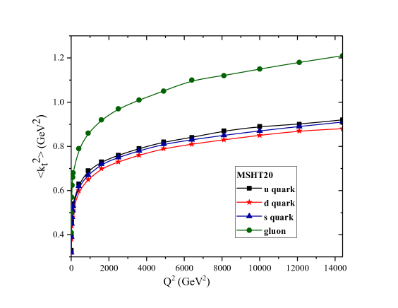
Figure 5: The average transverse momentum $<k_{t}^{2}>$ in the range $Q^{2}=2.4$ to $1.44\times 10^{4}$ $GeV^{2}$.

We perform the above calculations for light quarks and gluon in the range $Q^{2}=2.4$ to $1.44\times 10^{4}$ $GeV^{2}$ and the results are given in the table 1 and plotted in the figure 5. It is seen that for the light quarks the variation of $<k_{t}^{2}>$ with respect to $Q^{2}$ is approximately the same, while for gluon it becomes larger. This can be resulted from the general behavior of the gluon PDFs with respect to quarks ones.

Then, we repeat the above calculation (fitting the UPDFs to the equation (15)) for MMHT2014, CTEQ6l1, CJ15, HERAPDF15 and MSTW2008 PDFs sets selected from LHAPDF6 library LHAPDF . The results of these average transverse momenta for the light quarks are also shown in the figure 6 to see if the resulted average transverse momentum depends on the choice of different input PDFs sets. The similar behaviors with respect to various PDFs sets are found for u, d and s quarks.

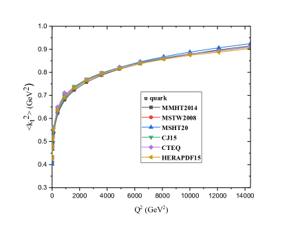
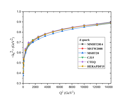
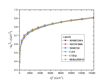
Figure 6: The plots of $<k_{t}^{2}>$ for the light quarks, using different PDFs sets: (a) u quark, (b) d quark, (c) s quark.

In addition we also explore the $x$ dependence of the average transverse momentum (Bacchetta, ) which are presented in the figure 7. There is a reasonable agreement between our result and those of reference (Bacchetta, ), especially in the higher $x$ values, considering the size of $<k_{t}^{2}>$ and this fact that we are not using any free parameter in our UPDFs beside the input PDFs sets.

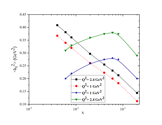
Figure 7: The plot of $<k_{t}^{2}>$ versus $x$ for the average transverse momentum of u quark (dotted curves) and those of reference (Bacchetta, ) (full curves).

III.3 The proton structure function in the $k_{t}$-factorization framework

For more detailed and precise studies, it is necessary to examine how the different UPDFs related to each PDFs sets, behave in the $k_{t}$-factorization phenomenological calculations in comparison to a corresponding measured observable, i.e., the $ep$ SIDIS experimental data. In recent years, the proton structure function can be measured with good accuracy up to the small $x$ values and the very high hard scale. So, we calculate and plot the proton structure functions, using the KMR UPDFs in the $k_{t}$-factorization framework with the different PDFs sets such as MSHT20, MMHT2014, MSTW2008, CJ15 and CTEQ6l1, for the two scales $Q^{2}=27$ and $90$ $GeV^{2}$ and compare the results with the experimental data of the NMC, ZEUS and H1+ZEUS collaborations in the figure 8. As one should expect there is good agreement between our predictions and the data at higher hard scale value, i.e., $90$ $GeV^{2}$. On the other hand there are not much difference between the various input PDFs sets (we do not consider other PDFs sets because of computer time consuming). The SF with PB TMDPDF (PB-NLO-HERAI+II-set2) PBTMD is also evaluated and plotted.

The gluon and quarks contribution to the SF of proton are plotted in the figures 9 and 10 to show their behaviors in terms of various PDFs sets. As one should expect , it is observed that the main contribution is comping from the gluon in the small $x$ region and again there are not much differences between the various PDFs sets. While the calculation with PB TMDPDFs give the smaller quarks distribution and larger gluon ones. This different behaviors are due to PB TMDPDFs which was discussed before in connection to the figure 3 and as it is claimed a global fitting is performed.

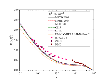
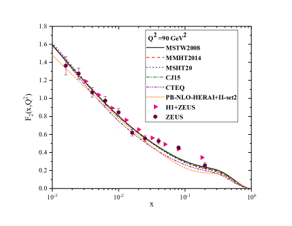
Figure 8: Compare the structure function for numerous sets of PDFs with experimental data in the scale (a) $Q^{2}=27$ $GeV^{2}$ and (b) $Q^{2}=90$ $GeV^{2}$.

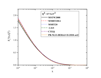
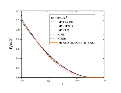
Figure 9: The gluon contribution to structure function of proton for numerous sets of PDFs in the scale (a) $Q^{2}=27$ $GeV^{2}$ and (b) $Q^{2}=90$ $GeV^{2}$.

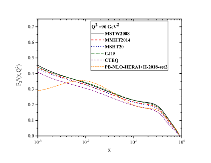
Figure 10: The quark contribution to structure function of proton for numerous sets of PDF in the scale (a) $Q^{2}=27$ $GeV^{2}$ and (b) $Q^{2}=90$ $GeV^{2}$.

Finally, we obtain and plot, the gluon contribution to the proton structure function using the Gaussian transverse momentum dependent, discussed in the section III.2 multiplied by corresponding PDFs sets in comparison with the KMR UPDFs input, see the figure 11. The average traverse momentum $<k_{t}^{2}>$ is used for the corresponding $x$ values and hard scale $Q^{2}$. We multiply $<k_{t}^{2}>$ by a constant, i.e., $a=39.5$ to get the best fit to KMR UPDFs SF at $Q^{2}=27$ $GeV^{2}$. It is seen that a reasonably result is achieved with the Gaussian assumption for the transverse dependent behavior of the UPDFs. Note that we use the same $a=39.5$ for the panel (b).

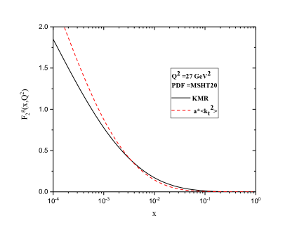
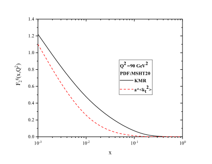
Figure 11: The comparison of gluon contribution to the structure function of proton, using KMR-UPDFs and Gaussian dependent transverse momentum (discussed in the section III.2) multiply by the corresponding PDFs set in the hard scale a) $Q^{2}=27$ $GeV^{2}$ and b) $Q^{2}=90$ $GeV^{2}$ with $a=39.5$.

IV Conclusions

In this work, we obtained the ratio of KMR UPDFs for the several sets of PDFs in the leading order with respect to the KMR UPDFs considering MMHT2014 PDFs set. It was shown that the KMR UPDFs with different input PDFs sets are almost very similar and stable (Modarres1, ). However the PB TMDPDFs have different behavior with respect to the KMR UPDFs, both by changing the hard scale and the transverse momentum.

In addition for the first time, we obtained the average transverse momentum in the high energy scales by fitting the $k_{t}$-dependent of the KMR UPDFs at each $x$ and $Q^{2}$ . It was shown that the average transverse momentum is not very sensitive to the longitudinal momentum fraction $x$, so one can average them with respect to $x$ at each scale $Q^{2}$. On the other hand, it does not have much variation regarding to the various quark flavours, i.e., they are almost the same for the light quarks, which is consistent to the results of references (Metz, ; Signori, ) (the section III.2). Its sensitivity considering the different input PDFs sets was also tested. The value of the average transverse momentum in the scale $Q^{2}=2.4$ $GeV^{2}$ is exactly within the range reported in the reference (Metz, ). However, it is greater than the one was fitted and used in the parton branching method, i.e., $0.125$ $GeV^{2}$ PBTMD .

In the section III.3, for a detailed examination, we calculated the proton structure function for a number of PDFs sets by using the KMR UPDFs and the $k_{t}$-factorization formalism and compared them with the experimental data. The results showed that the structure function calculated by KMR method is consistent with the experimental results and it is reasonably independent of the different PDFs sets used as the input. While the quarks and gluon contribution to proton SF using PB TMDPDFs, behave differently. Also we obtained the gluon contribution of the structure function using the KMR method and Gaussian transverse momentum dependent multiplied with corresponding PDFs sets, which showed a proper agreement using a constant variation for the best fitting.

We should make this remark that only the LO level analysis was performed in this report since it was intended to show the relative behaviors of different PDFs and UPDFs set. However the whole calculations can be extended to the NLO level. Therefore, in our future works, by calculating the NLO level contributions to the SF, we could have a better conclusion about the disagreement in the middle $x$ region of proton SF.

Appendix A J values

$$J_{1}=\frac{\kappa_{t}^{2}}{D_{1}^{2}}$$ (a-1)

$$J_{2}=\frac{1}{\sqrt{(D_{1}+k_{t}^{2})^{2}-4\kappa_{t}^{2}k_{t}^{2}}}-\frac{(D1+k_{t}^{2})(\beta(1-\beta)Q^{2}+m_{q}^{2})}{[(D_{1}+k_{t}^{2})^{2}-4\kappa_{t}^{2}k_{t}^{2}]^{3/2}}$$ (a-2)

$$J_{3}=\frac{1}{D_{1}}\left(1+\frac{\kappa_{t}^{2}-\beta(1-\beta)Q^{2}-m_{q}^{2}-k_{t}^{2}}{\sqrt{(D_{1}+k_{t}^{2})^{2}-4\kappa_{t}^{2}k_{t}^{2}}}\right)$$ (a-3)

$$J_{4}=\frac{1}{D_{1}^{2}}$$ (a-4)

$$J_{5}=\frac{D_{1}+k_{t}^{2}}{[(D_{1}+k_{t}^{2})^{2}-4\kappa_{t}^{2}k_{t}^{2}]^{3/2}}$$ (a-5)

$$J_{6}=\frac{2}{D_{1}}\frac{1}{\sqrt{(D_{1}+k_{t}^{2})^{2}-4\kappa_{t}^{2}k_{t}^{2}}}$$ (a-6)

That

$$D_{1}=\kappa_{t}^{2}+\beta(1-\beta)Q^{2}+m_{q}^{2}$$ (a-7)

Appendix B Refrences

ATLAS collaboration, arXive: 2112.11266v1 (2021).

Juan Rojo et al., J. Phys. G: Nucl. Part. Phys. 42, 103103 (2015).

CMS collaboration, arXive: 2109.13822v1 (2021).

V. N. Gribov and L. N. Lipatov, Yad. Fiz. 15, 781 (1972).

L. N. Lipatov, Sov. J. Nucl. Phys. 20, 94 (1975).

G. Altarelli and G. Parisi, Nucl. Phys. B 126, 298 (1977).

Y. L. Dokshitzer, Sov. Phys. JETP 46, 641 (1977).

E. A. Kuraev, L. N. Lipatov and V. S. Fadin, Sov. Phys. JETP 44, 433 (1976).

E. A. Kuraev, L. N. Lipatov and V. S. Fadin, ibid. 45, 199 (1977).

I. I. Balitskii and L. N. Lipatov, Sov. J. Nucl. Phys. 28, 822 (1978).

M. Ciafaloni, Nucl. Phys. B 296, 49 (1988).

S. Catani, F. Fiorani, and G. Marchesini, Phys. Lett. B 234, 339 (1990).

S. Catani, F. Fiorani, G. Marchesini, Nucl. Phys. B 336, 18 (1990).

G. Marchesini, Nucl. Phys. B 445, 49 (1995).

M. A. Kimber, A. D. Martin, M. G. Ryskin, Phys. Rev. D 63, 114027 (2001).

M.A. Kimber,”unintegrated parton distributions”, Ph.D. thesis, University of Durham (2001).

A. D. Martin, M. G. Ryskin, G. Watt, Eur. Phys. J. C 66, 163 (2010).

F. Hautmann, H. Jung, A. Lelek, V. Radescu and R. Zlebcik, JHEP 01, 070 (2018).

F. Hautmann, H. Jung, A. Lelek, V. Radescu and R. Zlebcik, Phys. Lett. B 772, 446 (2017).

A. Bermudez Martinez, P. Connor, H. Jung, A. Lelek, and R. Zlebcik, Phys. Rev. D 99, 074008 (2019).

M. Modarres and H. Hosseinkhani, Few-Body Syst. 47, 237 (2010).

H. Hosseinkhani and M. Modarres, Phys. Lett. B 694, 355 (2011).

H. Hosseinkhani and M. Modarres, Phys. Lett. B 708, 75 (2012).

H. Hosseinkhani, M. Modarres and N. Olanj, Int. J. Mod. Phys. A 32, 1750121 (2017).

M. Modarres, R. A. Nik, R. K. Valeshbadi, H. Hosseinkhani and N. Olanj, J. Phys. G 46, 105005 (2019)

M. Modarres, M. R. Masouminia, R. Aminzadeh Nik, H. Hosseinkhani and N. Olanj, Nucl. Phys. B 926, 406 (2018).

M. Modarres, M. R. Masouminia, R. Aminzadeh Nik, H. Hosseinkhani and N. Olanj, Nucl. Phys. B 922, 94 (2017).

R. K. Valeshabadi, M. Modarres and S. Rezaie, Eur. Phys. J. C 81, 961 (2021).

M. Modarres, R. Taghavi, R. A. Nik and R. K. Valeshabadi, Phys. Rev. D 104, 056005 (2021).

R. Kord Valeshabadi and M. Modarres, Eur. Phys. J. C 82, 66 (2022).

M. Modarres, H. Hosseinkhani and N. Olanj, Phys. Rev. D 89, 034015 (2014).

N. Olanj and M.Modarres, Eur. Phys. J. C 79 615(2019).

A. Bermudez Martinez et al., Eur. Phys. J. C 80, 598 (2020).

A. Metz and A. Vossen, Prog. Part. Nucl. Phys. 91, 136 (2016).

A. Signori, A. Bacchetta, M. Radicic and G. Schnelle, JHEP 11, 194 (2013).

M. G. Echevarria, A. Idilbi, Z. Kang and I. Vitev, Phys. Rev. D 89, 074013 (2014).

M. Anselmino, M. Boglione, J.O. Gonzalez, H. S. Melis and A. Prokudin, JHEP 04, 005 (2014).

M. Anselmino, M. Boglione, U. D’Alesio, A. Kotzinian, F. Murgia and A. Prokudin, Phys. Rev. D 71, 074006 (2005).

P. Schweitzer, T. Teckentrup and A. Metz, Phys. Rev. D 81, 094019 (2010).

M. Modarres and R. Taghavi, Phys.Rev.C 104, 114004 (2021).

M. Boglione, J.O. Gonzalez-Hermondez and R. Taghavi, Phys. Lett. B 772, 78 (2017).

NMC: Arneodo et al., Nucl. Phys. B 483, 3 (1997).

ZEUS: Derrick et al., Z. Phys. C 72, 399 (1996).

H1 and ZEUS Collaborations, JHEP 01, 109 (2010).

G. Marchesini, L. Cifarelli, Yu. L Dokshitzer, (eds.) Proceedings of the Workshop “QCD at 200 TeV”, Erice, Italy, p. 183. Plenum, New York (1992).

M. A. Kimber, J. Kwiecinski, A. D. Martin and A. M. Stasto, Phys. Rev. D 62, 094006 (2000).

Abdulov, N.A., Bacchetta, A., Baranov, S. et al., Eur. Phys. J. C 81, 752 (2021).

L. A. Harland-Langa, A. D. Martinb, P. Motylinskia and R.S. Thorne, Eur. Phys. J. C 75, 204 (2015).

A. Accardi, L. Brady, W. Melnitchouk, J. Owens and N. Sato, Phys. Rev. D 93, 114017 (2016).

J. Pumplin, D. R. Stump, J. Huston, H. L. Lai, P. Nadolsky and W. K. Tung, JHEP 07, 33 (2002).

J. M. Campbell, J. W. Huston, W. J. Stirling, Rept. Prog. Phys 70, 89 (2007).

A.D. Martin, W.J. Stirling, R.S. Thorne, G. Watt, Eur. Phys. J. C 63 189(2009).

S. Bailey, T. Cridge, L. A. Harland-Lang, A. D. Martin and R. S. Thorne, Eur. Phys. J. C 81, 341 (2021).

H1 and ZEUS Collaborations, Eur. Phys. J. C 75, 580 (2015).

A. Buckley, J. Ferrando and et al., Eur. Phys. J. C 75, 132 (2015).

A. Bacchetta, F. Delcarro, C. Pisano, M. Radici and A. Signori, JHEP 06, 071 (2017).