Dynamic CoVaR Modeling

Abstract

The popular systemic risk measure CoVaR (conditional Value-at-Risk) is widely used in economics and finance. Formally, it is defined as an (extreme) quantile of one variable (e.g., losses in the financial system) conditional on some other variable (e.g., losses in a bank’s shares) being in distress and, hence, measures the spillover of risks. In this article, we propose joint dynamic and semiparametric models for VaR and CoVaR together with a two-step M-estimator for the model parameters drawing on recently proposed bivariate scoring functions for the pair (VaR, CoVaR). Among others, this allows for the estimation of joint dynamic forecasting models for (VaR, CoVaR). We prove consistency and asymptotic normality of the proposed estimator and analyze its finite-sample properties in simulations. We apply our dynamic models to generate CoVaR forecasts for real financial data, which are shown to be superior to existing methods.

Keywords: CoVaR, Estimation, Forecasting, Modeling, Systemic Risk
JEL classification: C14 (Semiparametric and Nonparametric Methods); C22 (Time-Series Models); C58 (Financial Econometrics); G17 (Financial Forecasting and Simulation); G32 (Financial Risk and Risk Management)

1 Motivation

Since the introduction of the Value-at-Risk (VaR), risk forecasts have become a key input in financial decision making (Jorion, 2006). For instance, VaR and Expected Shortfall (ES) forecasts are now routinely used for setting capital requirements of financial institutions under the Basel framework (Liu and Stentoft, 2021). Consequently, a huge literature on forecasting VaR and ES has emerged (see, e.g., McNeil and Frey, 2000; Engle and Manganelli, 2004; Massacci, 2017; Patton et al., 2019). By definition, these measures are primarily designed to assess the riskiness of banks in isolation. Thus, these measures are well-suited to address microprudential objectives in banking regulation, that is, to limit risk taking of individual institutions.

However, in the aftermath of the financial crisis of 2007–09, macroprudential objectives have gained importance on the regulatory agenda (Acharya et al., 2012, 2017). While also attempting to limit risk taking of individual financial institutions, the macroprudential approach also takes into account the commonality of risk exposures among banks. For instance, a measure of interconnectedness of banks is now used under the Basel framework of the Basel Committee on Banking Supervision (2019, SCO40) to determine the global systemically important banks (G-SIBs), which are subjected to higher capital requirements. This new focus calls for systemic risk measures to accurately measure the interlinkages for which VaR and ES are unsuitable. Hence, a plethora of systemic risk measures is available by now (Giesecke and Kim, 2011; Chen et al., 2013; Adrian and Brunnermeier, 2016; Acharya et al., 2017).

One of the most popular systemic risk measures is the conditional VaR (CoVaR) of Adrian and Brunnermeier (2016). It is defined as a quantile of a financial loss (e.g., of an entire market), given a reference asset (e.g., a systemically important bank) is in distress, where the latter is measured as an exceedance of its VaR. Yet, while forecasting models and the asymptotic properties of forecasts are well explored for VaR and ES (Chan et al., 2007; Gao and Song, 2008; Wang and Zhao, 2016; Hoga, 2019), the models for CoVaR forecasting are hitherto rather ad-hoc and little is known about the consistency of the forecasts. In particular, DCC–GARCH models of Engle (2002) are popular due to their ability to accurately forecast conditional variance-covariance matrices (Laurent et al., 2012; Caporin and McAleer, 2014). However, as Francq and Zakoïan (2016, p. 620) point out, “[n]o formally established asymptotic results exist for the full estimation of the DCC […] models”; see also Darolles et al. (2018). This renders their use in forecasting systemic risk measures questionable. Moreover, there are additional problems associated with their use in systemic risk forecasting that stem from the non-uniqueness of the decomposition of the variance-covariance matrix (see Section 2.5). In sum, there is a need for multivariate models that can deliver accurate systemic risk forecasts with strong theoretical underpinnings.

The first main contribution of this paper is to introduce such dynamic, semiparametric models for the CoVaR, which we call CoCAViaR models, as they nest the classical CAViaR models of Engle and Manganelli (2004). In the spirit of Engle and Manganelli (2004) and Patton et al. (2019), we model the pair (VaR, CoVaR) depending on external covariates, past financial losses, and lagged (VaR, CoVaR). Our models are semiparametric in the sense that the quantities of interest (VaR and CoVaR) are modeled parametrically, yet no assumptions are placed on the remaining conditional distribution.

There are new challenges in modeling systemic risk vis-à-vis modeling univariate quantities such as VaR (Engle and Manganelli, 2004) and ES (Patton et al., 2019). Modeling VaR or (VaR, ES) requires to specify the univariate dynamics only. Yet, since CoVaR measures the interlinkage of bivariate random variables, it becomes necessary to model the co-movements as well. We explore different models for doing so, and identify several competitive performers in our empirical application.

Our second main contribution is to propose an estimator for the model parameters and derive its large sample properties. The main technical hurdle to overcome in developing asymptotic theory is that—unlike VaR and (VaR, ES)—the pair (VaR, CoVaR) fails to be elicitable, such that no real-valued scoring function exists that is uniquely minimized by the true report (Fissler and Hoga, 2022). This renders standard M-estimation—adopted by Engle and Manganelli (2004), Dimitriadis and Bayer (2019) and Patton et al. (2019)—infeasible (Dimitriadis et al., 2022, Theorem 1). Instead, we exploit the multi-objective elicitability of (VaR, CoVaR) (Fissler and Hoga, 2022). This property suggests a two-step M-estimator. In the first step, the score in the VaR component is minimized, and then the CoVaR score is minimized in the second step. We show consistency and asymptotic normality of our two-step M-estimator and propose valid inference based on consistent estimation of the asymptotic variance-covariance matrix. Our proofs show how to deal with non-smooth and discontinuous objective functions in the context of two-step M-estimation for dynamic models (based on past model values). We speculate that our proof strategy may also be used elsewhere and, therefore, may be of independent interest. We provide an open source R package (Dimitriadis and Hoga, 2022) that contains the implementation of our two-step M-estimator together with inference tools for the flexible class of dynamic CoVaR models.

Simulations confirm the good finite-sample properties of our estimator. While the parameters of the CoCAViaR models can be estimated accurately in realistic settings, reliable inference for the model parameters requires large sample sizes or moderate probability levels. However, as the main use of our CoCAViaR models is in forecasting, inference for the model parameters is of lesser importance than consistent estimates.

In the empirical application, we compare CoVaR forecasts issued from our CoCAViaR models with those from benchmark DCC–GARCH models. We do so for the four most systemically risky US banks according to the Financial Stability Board (2021), whose impact on a broader market index is assessed by CoVaR. Our various CoCAViaR model specifications tend to outperform the DCC–GARCH benchmarks, particularly in the CoVaR forecasts but also in the VaR component. Often, these differences in predictive ability are also statistically significant, as judged by the Diebold and Mariano (1995)-type comparative backtest of Fissler and Hoga (2022). The superiority of our proposals may be explained by two reasons. First, our CoCAViaR specifications are specifically tailored to model the quantities of interest (VaR and CoVaR), whereas multivariate GARCH processes focus on modeling the complete predictive distribution. Second, our estimation technique is tailored to provide an accurate description of the (VaR, CoVaR) evolution. In particular, the estimator is not too strongly influenced by center-of-the-distribution observations as, e.g., standard estimators of multivariate GARCH models.

The rest of the paper is structured as follows. Section 2 formally introduces CoVaR, our modeling framework and the appertaining parameter estimator. It also gives large sample results for our estimator, and points out the difficulties of DCC–GARCH models to predict CoVaR. We illustrate the finite-sample properties of our estimator in Section 3. Section 4 presents the empirical application. The final Section 5 concludes. The main proofs are relegated to the Appendix, and additional details are given in the Supplementary Material, which also verifies our model assumptions for CCC–GARCH models and generalizes our consistency result to arbitrary starting values.

2 Modeling and Estimation

2.1 The CoVaR

Throughout the paper, we consider a sample of size $n\in\mathbb{N}$ of the bivariate series $\big{\{}(X_{t},Y_{t})^{\prime}\big{\}}_{t\in\mathbb{N}}$. Specifically, $Y_{t}$ stands for the log-losses of interest (e.g., system-wide losses in the financial system) and $X_{t}$ are the log-losses of some reference position (e.g., the losses of a bank’s shares). Here, log-losses are simply the negated log-returns. Let $\mathcal{F}_{t}$ denote some time-$t$ information set to be specified below. Define $\operatorname{VaR}_{t,\beta}=\operatorname{VaR}_{\beta}(F_{X_{t}\mid\mathcal{F}_{t-1}})$, where $\operatorname{VaR}_{\beta}(F)=F^{-1}(\beta)$ with $\beta\in[0,1)$ denotes the $\beta$-quantile of the (absolutely continuous) distribution $F$, and $F_{X_{t}\mid\mathcal{F}_{t-1}}$ denotes the conditional distribution of $X_{t}$ given $\mathcal{F}_{t-1}$. The stress event that is considered in the definition of the CoVaR is that the loss of the reference position exceeds its VaR, i.e., $\{X_{t}\geq\operatorname{VaR}_{t,\beta}\}$. With our orientation of $X_{t}$ denoting financial losses, we commonly consider values for $\beta$ close to one, such as $\beta=0.95$. For $\alpha\in(0,1)$ we define $\operatorname{CoVaR}_{t,\alpha|\beta}=\operatorname{CoVaR}_{\alpha|\beta}(F_{(X_{t},Y_{t})^{\prime}\mid\mathcal{F}_{t-1}})$, where

$$\operatorname{CoVaR}_{\alpha|\beta}(F_{X,Y})=\operatorname{VaR}_{\alpha}(F_{Y\mid X\geq\operatorname{VaR}_{\beta}(F_{X})})$$

for a joint distribution function $F_{X,Y}$ with marginals $F_{X}$ and $F_{Y}$. Again, we usually consider values of $\alpha$ close to one. If $\alpha=\beta$ we simply write $\operatorname{CoVaR}_{t,\alpha}=\operatorname{CoVaR}_{t,\alpha|\alpha}$, and for $\beta=0$ we simply have $\operatorname{CoVaR}_{t,\alpha|\beta}=\operatorname{VaR}_{\alpha}(F_{Y_{t}\mid\mathcal{F}_{t-1}})$. Note that our definition of CoVaR deviates from the original one of Adrian and Brunnermeier (2016), who used $\{X_{t}=\operatorname{VaR}_{t,\beta}\}$ as the stress event. This latter choice is problematic because it often has probability zero and it does not fully incorporate all tail events of $X_{t}$. Thus, we follow Girardi and Tolga Ergün (2013) and Nolde and Zhang (2020) in using the above alternative definition.

2.2 Dynamic Models for VaR and CoVaR

In the spirit of Engle and Manganelli (2004) and Patton et al. (2019), we consider semiparametric models for the pair (VaR, CoVaR) of the general form

$$\begin{pmatrix}v_{t}(\bm{\theta}^{v})\\ c_{t}(\bm{\theta}^{c})\end{pmatrix}=\begin{pmatrix}v_{t}\big{(}(X_{t-1},Y_{t-1})^{\prime},\bm{Z}_{t-1},\ldots,(X_{1},Y_{1})^{\prime},\bm{Z}_{1},v_{0}(\bm{\theta}^{v});\bm{\theta}^{v}\big{)}\\ c_{t}\big{(}(X_{t-1},Y_{t-1})^{\prime},\bm{Z}_{t-1},\ldots,(X_{1},Y_{1})^{\prime},\bm{Z}_{1},c_{0}(\bm{\theta}^{c});\bm{\theta}^{c}\big{)}\end{pmatrix},\qquad t\in\mathbb{N},$$ (1)

where $\bm{Z}_{t-1}$ is some (possibly multivariate) exogenous covariate vector. Throughout the paper, we assume that the model in (1) is correctly specified in the sense that there exist true parameter values $\bm{\theta}^{v}_{0}\in\bm{\varTheta}^{v}\subset\mathbb{R}^{p}$ and $\bm{\theta}^{c}_{0}\in\bm{\varTheta}^{c}\subset\mathbb{R}^{q}$ such that

$$\begin{pmatrix}\operatorname{VaR}_{t,\beta}\\ \operatorname{CoVaR}_{t,\alpha\mid\beta}\end{pmatrix}=\begin{pmatrix}v_{t}(\bm{\theta}_{0}^{v})\\ c_{t}(\bm{\theta}_{0}^{c})\end{pmatrix}$$ (2)

almost surely (a.s.), where $\mathcal{F}_{t-1}=\sigma\big{(}(X_{t-1},Y_{t-1})^{\prime},\bm{Z}_{t-1},(X_{t-2},Y_{t-2})^{\prime},\bm{Z}_{t-2},\ldots\big{)}$.

A few comments on our modeling approach are in order. First, the fact that the VaR model $v_{t}(\cdot)$ does not depend on the CoVaR parameters $\bm{\theta}^{c}$ renders our two-step estimator (introduced in the next subsection) feasible; see Section 2.3 for more detail. In contrast, our two-step estimator is in principle compatible with letting $c_{t}(\cdot)$ depend on $\bm{\theta}^{v}$. This would, however, come at the cost of a further explosion of technicality in the proofs, without any offsetting improvements (in terms of predictive accuracy) of the resulting models; see the empirical application in Section 4.

Second, our model is semiparametric in the sense that—while the model dynamics are governed by the parameters $\bm{\theta}^{v}$ and $\bm{\theta}^{c}$—we impose no additional distributional assumption on the innovations driving the evolution of $(X_{t},Y_{t})^{\prime}$.

Third, besides the full history of lagged values of $X_{t}$, $Y_{t}$ and $\bm{Z}_{t}$, the model in (1) depends on the (correctly specified) initial values $v_{0}(\bm{\theta}^{v})$ and $c_{0}(\bm{\theta}^{c})$. Thus, our setup allows for the inclusion of lagged (VaR, CoVaR); see Example 1 below for details. Equivalently, the model could be defined to depend on the infinite past of $X_{t}$, $Y_{t}$ and $\bm{Z}_{t}$, which would be in line with the rest of the related literature developing dynamic models for quantile-related quantities (Engle and Manganelli, 2004; White et al., 2015; Patton et al., 2019; Catania and Luati, 2022). However, in contrast to the extant literature, our definition in (1) allows for a clearer discussion of the implications of starting values for estimation; see also Remark 1.

Fourth, the model in (1) generalizes classical (time-series) quantile regressions based on lagged values of $X_{t}$, $Y_{t}$ and the covariate vector $\bm{Z}_{t}$. Also, the “VAR for VaR” models (of dimension two) of White et al. (2015) are nested by choosing $\beta=0$ such that the CoVaR simply becomes the VaR of $Y_{t}$.

Example 1.

The general formulation of our model class in (1) allows for dynamic models, where (VaR, CoVaR) may depend on their lags. E.g., it nests models of the form

$$\begin{pmatrix}v_{t}(\bm{\theta}^{v})\\ c_{t}(\bm{\theta}^{c})\end{pmatrix}=\bm{\omega}+\bm{A}\begin{pmatrix}|X_{t-1}|\\ |Y_{t-1}|\end{pmatrix}+\bm{B}\begin{pmatrix}v_{t-1}(\bm{\theta}^{v})\\ c_{t-1}(\bm{\theta}^{c})\end{pmatrix}$$ (3)

with parameters $\bm{\omega}\in\mathbb{R}^{2}$, $\bm{A},\bm{B}\in\mathbb{R}^{2\times 2}$ that can be collected in $\bm{\theta}^{v}$ and $\bm{\theta}^{c}$. Borrowing terminology from Engle and Manganelli (2004), we call models of the form (3) Symmetric Absolute Value (SAV) CoCAViaR models. Of course, our restriction that $v_{t}(\cdot)$ ($c_{t}(\cdot)$) only depends on $\bm{\theta}^{v}$ ($\bm{\theta}^{c}$) implies that the matrix $\bm{B}=(B_{ij})_{i,j=1,2}$ is diagonal (i.e., $B_{12}=B_{21}=0$) to facilitate two-step M-estimation.

The models of Example 1 are correctly specified under a type of Jeantheau’s (1998) extended constant conditional correlation (ECCC) process, that has been studied extensively in the literature (He and Teräsvirta, 2004; Conrad and Karanasos, 2010):

$$\begin{pmatrix}X_{t}\\ Y_{t}\end{pmatrix}=\begin{pmatrix}\sigma_{X,t}\,\varepsilon_{X,t}\\ \sigma_{Y,t}\,\varepsilon_{Y,t}\end{pmatrix},\qquad\begin{pmatrix}\sigma_{X,t}\\ \sigma_{Y,t}\end{pmatrix}=\widetilde{\bm{\omega}}+\widetilde{\bm{A}}\begin{pmatrix}|X_{t-1}|\\ |Y_{t-1}|\end{pmatrix}+\widetilde{\bm{B}}\begin{pmatrix}\sigma_{X,t-1}\\ \sigma_{Y,t-1}\end{pmatrix},$$ (4)

where $\widetilde{\bm{\omega}}\in\mathbb{R}^{2}$, $\widetilde{\bm{A}},\widetilde{\bm{B}}\in\mathbb{R}^{2\times 2}$. In (4), the $\mathcal{F}_{t-1}$-measurable conditional volatilities $\sigma_{X,t}$ and $\sigma_{Y,t}$ are independent of the independent and identically distributed (i.i.d.) innovations $\big{(}\varepsilon_{X,t},\varepsilon_{Y,t}\big{)}^{\prime}\overset{\text{i.i.d.}}{\sim}F\big{(}\bm{0},\bm{\varSigma}\big{)}$, where $F$ denotes a generic absolutely continuous, bivariate distribution with zero mean and covariance matrix $\bm{\varSigma}=\begin{pmatrix}1&\rho\\ \rho&1\end{pmatrix}$, $\rho\in(-1,1)$. We deviate from Jeantheau (1998) by using absolute (instead of squared) returns as drivers of volatility, since these have more predictive content for volatility (Forsberg and Ghysels, 2007). Model (4) implies the (VaR, CoVaR) dynamics in (3), where the true model parameters $\bm{\omega}_{0},\bm{A}_{0},\bm{B}_{0}$ of the model in (3) arise as transformations of $\widetilde{\bm{\omega}},\widetilde{\bm{A}},\widetilde{\bm{B}}$.

In our simulations in Section 3, we use (a restricted version of) model (4) to generate data to assess how well our two-step M-estimator performs. In our empirical application, we consider various SAV CoCAViaR specifications based on zero restrictions in $\bm{A}$ and $\bm{B}$ as well as generalizations to so-called “asymmetric slope” models based on the positive and negative components of $X_{t}$ and $Y_{t}$ instead of on their absolute values.

2.3 Parameter Estimation

We now introduce estimators of the unknown parameters $\bm{\theta}_{0}^{v}$ and $\bm{\theta}_{0}^{c}$. As we consider M-estimation in this paper, we require a to-be-minimized objective (or also: scoring) function. However, as pointed out in the Motivation, there is no real-valued scoring function associated with the pair (VaR, CoVaR). Dimitriadis et al. (2022, Theorem 1) show that the existence of such a (consistent) scoring function is a necessary condition for consistent M-estimation of semiparametric models. To overcome this drawback, Fissler and Hoga (2022) propose to consider a $\mathbb{R}^{2}$-valued scoring function in the closely related context of forecast evaluation. To be able to compare forecasts, $\mathbb{R}^{2}$ has to be equipped with an order, and Fissler and Hoga (2022) show that the lexicographic order is suitable for that purpose. Specifically, they show that (under some regularity conditions) the expectation of the $\mathbb{R}^{2}$-valued scoring function

$$\bm{S}\Bigg{(}\begin{pmatrix}v\\ c\end{pmatrix},\begin{pmatrix}x\\ y\end{pmatrix}\Bigg{)}=\begin{pmatrix}S^{\operatorname{VaR}}(v,x)\\ S^{\operatorname{CoVaR}}\big{(}(v,c)^{\prime},(x,y)^{\prime}\big{)}\end{pmatrix}=\begin{pmatrix}[\mathds{1}_{\{x\leq v\}}-\beta][v-x]\\ \mathds{1}_{\{x>v\}}[\mathds{1}_{\{y\leq c\}}-\alpha][c-y]\end{pmatrix}$$ (5)

is minimized by the true VaR and CoVaR with respect to the lexicographic order. That is, for all $v,c\in\mathbb{R}$,

$$\mathbb{E}\Bigg{[}\bm{S}\Bigg{(}\begin{pmatrix}\operatorname{VaR}_{\beta}(F_{X})\\ \operatorname{CoVaR}_{\alpha\mid\beta}(F_{X,Y})\end{pmatrix},\begin{pmatrix}X\\ Y\end{pmatrix}\Bigg{)}\Bigg{]}\preceq_{\operatorname{lex}}\mathbb{E}\Bigg{[}\bm{S}\Bigg{(}\begin{pmatrix}v\\ c\end{pmatrix},\begin{pmatrix}X\\ Y\end{pmatrix}\Bigg{)}\Bigg{]},$$

where $(x_{1},x_{2})^{\prime}\preceq_{\operatorname{lex}}(y_{1},y_{2})^{\prime}$ if $x_{1}<y_{1}$ or ($x_{1}=y_{1}$ and $x_{2}\leq y_{2}$). Note that $S^{\operatorname{VaR}}(\cdot,\cdot)$ in (5) is the standard tick-loss function known from quantile regression. Clearly, $S^{\operatorname{CoVaR}}(\cdot,\cdot)$ is similar in structure to $S^{\operatorname{VaR}}(\cdot,\cdot)$, with the only difference being the indicator $\mathds{1}_{\{x>v\}}$ that restricts the evaluation to observations with VaR exceedances in the first component. In the related literature, these scoring functions are often also called loss functions (Gneiting, 2011). To avoid confusion with financial “losses”, we adhere to the term “scoring function”.

The definition of the lexicographic order suggests the following two-step M-estimator of $\bm{\theta}_{0}^{v}$ and $\bm{\theta}_{0}^{c}$. In the first step, we use

$$\widehat{\bm{\theta}}_{n}^{v}=\operatorname*{arg\,min}_{\bm{\theta}^{v}\in\bm{\varTheta}^{v}}\frac{1}{n}\sum_{t=1}^{n}S^{\operatorname{VaR}}\big{(}v_{t}(\bm{\theta}^{v}),X_{t}\big{)},$$

such that the parameters are chosen to minimize the average empirical score in the VaR component for some parameter space $\bm{\varTheta}^{v}\subset\mathbb{R}^{p}$. For the VaR model $v_{t}(\cdot)$, this is the quantile regression estimator of Engle and Manganelli (2004).

With the estimate $\widehat{\bm{\theta}}_{n}^{v}$ at hand, the lexicographic order then suggests to minimize the average empirical score in the second component via

$$\widehat{\bm{\theta}}_{n}^{c}=\operatorname*{arg\,min}_{\bm{\theta}^{c}\in\bm{\varTheta}^{c}}\frac{1}{n}\sum_{t=1}^{n}S^{\operatorname{CoVaR}}\Big{(}\big{(}v_{t}(\widehat{\bm{\theta}}_{n}^{v}),c_{t}(\bm{\theta}^{c})\big{)}^{\prime},\big{(}X_{t},Y_{t}\big{)}^{\prime}\Big{)}$$

for some CoVaR parameter space $\bm{\varTheta}^{c}\subset\mathbb{R}^{q}$. For this two-step estimator to be feasible, the requirement that the VaR evolution does not depend on $\bm{\theta}^{c}$ is essential. Section 2.4.2 shows that the presence of $\widehat{\bm{\theta}}_{n}^{v}$ in the minimization problem impacts the asymptotic variance of $\widehat{\bm{\theta}}_{n}^{c}$. Of course, this is usually the case for two-step estimators (Newey and McFadden, 1994, Section 6).

2.4 Asymptotic Properties of the Estimators

2.4.1 Consistency

We first show consistency of our two-step M-estimators $\widehat{\bm{\theta}}_{n}^{v}$ and $\widehat{\bm{\theta}}_{n}^{c}$. To do so, we introduce several regularity conditions in Assumption 1, where $K<\infty$ is some large positive constant, and $\mathinner{\!\left\lVert\bm{x}\right\rVert}$ denotes the Euclidean norm when $\bm{x}$ is a vector, and the Frobenius norm when $\bm{x}$ is matrix-valued. The joint cumulative distribution function (c.d.f.) of $(X_{t},Y_{t})^{\prime}\mid\mathcal{F}_{t-1}$ is denoted by $F_{t}(\cdot,\cdot)$, and its Lebesgue density (which we assume exists) by $f_{t}(\cdot,\cdot)$. Similarly, $F_{t}^{W}(\cdot)$ ($f_{t}^{W}(\cdot)$) denotes the distribution (density) function of $W_{t}\mid\mathcal{F}_{t-1}$ for $W\in\{X,Y\}$. For sufficiently smooth functions $\mathbb{R}^{p}\ni\bm{\theta}\mapsto f(\bm{\theta})\in\mathbb{R}$, we denote the $(p\times 1)$-gradient by $\nabla f(\bm{\theta})$, its transpose by $\nabla^{\prime}f(\bm{\theta})$ and the $(p\times p)$-Hessian by $\nabla^{2}f(\bm{\theta})$.

Assumption 1.

1. The models $v_{t}(\cdot)$ and $c_{t}(\cdot)$ are correctly specified in the sense of (2). Furthermore, $\mathbb{P}\big{\{}v_{t}(\bm{\theta}^{v})=v_{t}(\bm{\theta}_{0}^{v})\big{\}}=1$ for all $t\in\mathbb{N}$ implies that $\bm{\theta}^{v}=\bm{\theta}_{0}^{v}$, and $\mathbb{P}\big{\{}c_{t}(\bm{\theta}^{c})=c_{t}(\bm{\theta}_{0}^{c})\big{\}}=1$ for all $t\in\mathbb{N}$ implies that $\bm{\theta}^{c}=\bm{\theta}_{0}^{c}$.

2. $\big{\{}(X_{t},Y_{t},\bm{Z}_{t}^{\prime})^{\prime}\big{\}}_{t\in\mathbb{N}}$ is strictly stationary.

3. For all $t\in\mathbb{N}$, $F_{t}(\cdot,\cdot)$ belongs to a class of distributions on $\mathbb{R}^{2}$ that possesses a positive Lebesgue density for all $(x,y)^{\prime}\in\mathbb{R}^{2}$ such that $F_{t}(x,y)\in(0,1)$. Moreover, $f_{t}^{X}(\cdot)\leq K$ for all $t\in\mathbb{N}$.

4. $\bm{\varTheta}=\bm{\varTheta}^{v}\times\bm{\varTheta}^{c}$ is compact, where $\bm{\varTheta}^{v}\subset\mathbb{R}^{p}$ and $\bm{\varTheta}^{c}\subset\mathbb{R}^{q}$.

5. $\Big{\{}\bm{S}\Big{(}\big{(}v_{t}(\bm{\theta}^{v}),c_{t}(\bm{\theta}^{c})\big{)}^{\prime},(X_{t},Y_{t})^{\prime}\Big{)}\Big{\}}_{t\in\mathbb{N}}$ obeys the uniform law of large numbers (ULLN) in $(\bm{\theta}^{v\prime},\bm{\theta}^{c\prime})^{\prime}\in\bm{\varTheta}$.

6. For all $t\in\mathbb{N}$, $v_{t}(\bm{\theta}^{v})$ and $c_{t}(\bm{\theta}^{c})$ are $\mathcal{F}_{t-1}$-measurable and a.s. continuous in $\bm{\theta}^{v}$ and $\bm{\theta}^{c}$.

7. For all $t\in\mathbb{N}$, $v_{t}(\bm{\theta}^{v})$ is continuously differentiable on $\operatorname{int}(\bm{\varTheta}^{v})$.

8. There exists a neighborhood of $\bm{\theta}_{0}^{v}$, such that $\mathinner{\!\left\lVert\nabla v_{t}(\bm{\theta}^{v})\right\rVert}\leq V_{1}(\mathcal{F}_{t-1})$ for all elements $\bm{\theta}^{v}$ of that neighborhood. Furthermore, $|v_{t}(\bm{\theta}^{v})|\leq V(\mathcal{F}_{t-1})$ for all $\bm{\theta}^{v}\in\bm{\varTheta}^{v}$, and $|c_{t}(\bm{\theta}^{c})|\leq C(\mathcal{F}_{t-1})$ for all $\bm{\theta}^{c}\in\bm{\varTheta}^{c}$.

9. $\mathbb{E}\big{[}V(\mathcal{F}_{t-1})\big{]}\leq K$, $\mathbb{E}\big{[}V_{1}(\mathcal{F}_{t-1})\big{]}\leq K$, $\mathbb{E}\big{[}V_{1}(\mathcal{F}_{t-1})C(\mathcal{F}_{t-1})\big{]}\leq K$, $\mathbb{E}|X_{t}|\leq K$, $\mathbb{E}|Y_{t}|^{1+\iota}\leq K$ for some $\iota>0$.

In Assumption 1, item (i) ensures identification of the true parameters and item (ii) is a standard stationarity condition. Item (iii) ensures—among other things—strict (multi-objective) consistency of the scoring function given in (5); see Fissler and Hoga (2022, Theorem 4.2) for details. Compactness in (iv) is a standard requirement in extremum estimation; see Newey and McFadden (1994). Assumption 1 (v) is also a standard condition, imposed for instance by Engle and Manganelli (2004, Assumption C6) and Patton et al. (2019, Assumption 1 (A)). It can be verified using, e.g., Lemma 2.8 in Newey and McFadden (1994) or Theorem 21.9 in Davidson (1994). The final items (vi)–(ix) are smoothness conditions on the model. See Remark 3 and Supplement G for a verification of these conditions for CCC–GARCH models of Bollerslev (1990).

Our first main theoretical result establishes the consistency of $\widehat{\bm{\theta}}_{n}^{v}$ and $\widehat{\bm{\theta}}_{n}^{c}$:

Theorem 1.

Suppose Assumption 1 holds. Then, as $n\to\infty$, $\widehat{\bm{\theta}}_{n}^{v}\overset{\mathbb{P}}{\longrightarrow}\bm{\theta}_{0}^{v}$ and $\widehat{\bm{\theta}}_{n}^{c}\overset{\mathbb{P}}{\longrightarrow}\bm{\theta}_{0}^{c}$.

The proof of Theorem 1 proceeds by verifying the conditions of Theorem 2.1 in Newey and McFadden (1994), and can be found in Appendix A. The result that $\widehat{\bm{\theta}}_{n}^{v}\overset{\mathbb{P}}{\longrightarrow}\bm{\theta}_{0}^{v}$ is essentially a version of Theorem 1 in Engle and Manganelli (2004); the only difference being that our regularity conditions are slightly more involved, since we also show that $\widehat{\bm{\theta}}_{n}^{c}\overset{\mathbb{P}}{\longrightarrow}\bm{\theta}_{0}^{c}$.

Remark 1.

By imposing (2), we follow the related literature on dynamic quantile models (Engle and Manganelli, 2004; White et al., 2015; Patton et al., 2019; Catania and Luati, 2022) and assume that the true starting values $v_{0}(\bm{\theta}^{v})$ and $c_{0}(\bm{\theta}^{c})$ are known. We generalize the consistency result of Theorem 1 in Supplement F to arbitrary starting values for an empirically relevant model class that is linear in the lagged model values, nests the models in (3) and contains all models used in our simulations and empirical application. For this result, it essentially suffices to extend Assumption 1 by the well-known condition that the spectral radius of the parameter matrix $\bm{B}$ in (3) is strictly smaller one. We mention that starting values are of concern only in autoregressive-type models. For moving average-type models (e.g., model (3) with $\bm{B}=\bm{0}$) they are irrelevant.

2.4.2 Asymptotic Normality

To show asymptotic normality of our estimators, we have to impose additional regularity conditions on the model. We denote the partial derivative of $F_{t}(\cdot,\cdot)$ with respect to the $i$-th argument by $\partial_{i}F_{t}(\cdot,\cdot)$ for $i=1,2$.

Assumption 2.

1. $\bm{\theta}_{0}^{v}\in\operatorname{int}(\bm{\varTheta}^{v})$ and $\bm{\theta}_{0}^{c}\in\operatorname{int}(\bm{\varTheta}^{c})$, where $\operatorname{int}(\cdot)$ denotes the interior of a set.

2. $v_{t}(\cdot)$ and $c_{t}(\cdot)$ are a.s. twice continuously differentiable on $\operatorname{int}(\bm{\varTheta}^{v})$ and $\operatorname{int}(\bm{\varTheta}^{c})$, respectively.

3. There exists a neighborhood of $\bm{\theta}_{0}^{v}$, such that $\mathinner{\!\left\lVert\nabla^{2}v_{t}(\bm{\theta}^{v})\right\rVert}\leq V_{2}(\mathcal{F}_{t-1})$, $\mathinner{\!\left\lVert\nabla^{2}v_{t}(\bm{\theta}^{v})-\nabla^{2}v_{t}(\bm{\tau}^{v})\right\rVert}\leq V_{3}(\mathcal{F}_{t-1})\mathinner{\!\left\lVert\bm{\theta}^{v}-\bm{\tau}^{v}\right\rVert}$ for all elements $\bm{\theta}^{v}$, $\bm{\tau}^{v}$ of that neighborhood.

4. There exists a neighborhood of $\bm{\theta}_{0}^{c}$, such that $\mathinner{\!\left\lVert\nabla c_{t}(\bm{\theta}^{c})\right\rVert}\leq C_{1}(\mathcal{F}_{t-1})$, $\mathinner{\!\left\lVert\nabla^{2}c_{t}(\bm{\theta}^{c})\right\rVert}\leq C_{2}(\mathcal{F}_{t-1})$, $\mathinner{\!\left\lVert\nabla^{2}c_{t}(\bm{\theta}^{c})-\nabla^{2}c_{t}(\bm{\tau}^{c})\right\rVert}\leq C_{3}(\mathcal{F}_{t-1})\mathinner{\!\left\lVert\bm{\theta}^{c}-\bm{\tau}^{c}\right\rVert}$ for all elements $\bm{\theta}^{c}$, $\bm{\tau}^{c}$ of that neighborhood.

5. There exists some $\iota>0$, such that $\mathbb{E}\big{[}V_{1}^{3+\iota}(\mathcal{F}_{t-1})\big{]}\leq K$, $\mathbb{E}\big{[}V_{2}^{(3+\iota)/2}(\mathcal{F}_{t-1})\big{]}\leq K$, $\mathbb{E}\big{[}V_{3}(\mathcal{F}_{t-1})\big{]}\leq K$, $\mathbb{E}\big{[}C_{1}^{3+\iota}(\mathcal{F}_{t-1})\big{]}\leq K$, $\mathbb{E}\big{[}C_{2}^{(3+\iota)/2}(\mathcal{F}_{t-1})\big{]}\leq K$, $\mathbb{E}\big{[}C_{3}(\mathcal{F}_{t-1})\big{]}\leq K$.

6. $\big{|}f_{t}^{X}(x)-f_{t}^{X}(x^{\prime})\big{|}\leq K|x-x^{\prime}|$, $\big{|}f_{t}^{Y}(y)-f_{t}^{Y}(y^{\prime})\big{|}\leq K|y-y^{\prime}|$, $\big{|}\partial_{1}F_{t}(x,y)-\partial_{1}F_{t}(x^{\prime},y)\big{|}\leq K|x-x^{\prime}|$, and $\big{|}\partial_{2}F_{t}(x,y)-\partial_{2}F_{t}(x,y^{\prime})\big{|}\leq K|y-y^{\prime}|$ for all $x,x^{\prime},y,y^{\prime}$ in the support of $F_{t}(\cdot,\cdot)$.

7. $f_{t}^{Y}(\cdot)\leq K$, $f_{t}(\cdot,\cdot)\leq K$, $\big{|}\partial_{i}F_{t}(\cdot,\cdot)\big{|}\leq K$ for $i=1,2$.

8. The matrices

   $$\bm{\varLambda} =\mathbb{E}\Big{[}f_{t}^{X}\big{(}v_{t}(\bm{\theta}_{0}^{v})\big{)}\nabla v_{t}(\bm{\theta}_{0}^{v})\nabla^{\prime}v_{t}(\bm{\theta}_{0}^{v})\Big{]}\in\mathbb{R}^{p\times p},$$

   $$\bm{\varLambda}_{(1)} =\mathbb{E}\bigg{\{}\nabla c_{t}(\bm{\theta}_{0}^{c})\nabla^{\prime}c_{t}(\bm{\theta}_{0}^{c})\Big{[}f_{t}^{Y}\big{(}c_{t}(\bm{\theta}_{0}^{c})\big{)}-\partial_{2}F_{t}\big{(}v_{t}(\bm{\theta}_{0}^{v}),c_{t}(\bm{\theta}_{0}^{c})\big{)}\Big{]}\bigg{\}}\in\mathbb{R}^{q\times q},$$

   $$\bm{V} =\beta(1-\beta)\mathbb{E}\big{[}\nabla v_{t}(\bm{\theta}_{0}^{v})\nabla^{\prime}v_{t}(\bm{\theta}_{0}^{v})\big{]}\in\mathbb{R}^{p\times p},$$

   $$\bm{C}^{\ast} =\alpha(1-\alpha)(1-\beta)\mathbb{E}\big{[}\nabla c_{t}(\bm{\theta}_{0}^{c})\nabla^{\prime}c_{t}(\bm{\theta}_{0}^{c})\big{]}\in\mathbb{R}^{q\times q}$$

   are positive definite, and

   $$\bm{\varLambda}_{(2)} =\mathbb{E}\bigg{\{}\nabla c_{t}(\bm{\theta}_{0}^{c})\nabla^{\prime}v_{t}(\bm{\theta}_{0}^{v})\Big{[}\alpha f_{t}^{X}\big{(}v_{t}(\bm{\theta}_{0}^{v})\big{)}-\partial_{1}F_{t}\big{(}v_{t}(\bm{\theta}_{0}^{v}),c_{t}(\bm{\theta}_{0}^{c})\big{)}\Big{]}\bigg{\}}\in\mathbb{R}^{q\times p}$$

   has full rank.

9. $\sup_{\bm{\theta}^{v}\in\bm{\varTheta}^{v}}\sum_{t=1}^{n}\mathds{1}_{\big{\{}X_{t}=v_{t}(\bm{\theta}^{v})\big{\}}}=O(1)$ and $\sup_{\bm{\theta}^{c}\in\bm{\varTheta}^{c}}\sum_{t=1}^{n}\mathds{1}_{\big{\{}Y_{t}=c_{t}(\bm{\theta}^{c})\big{\}}}=O(1)$ a.s., as $n\to\infty$.

10. $\Big{\{}\big{(}X_{t},\ Y_{t},\ \bm{Z}_{t}^{\prime},\ v_{t}(\bm{\theta}_{0}^{v}),\ \nabla^{\prime}v_{t}(\bm{\theta}_{0}^{v}),\ c_{t}(\bm{\theta}_{0}^{c}),\ \nabla^{\prime}c_{t}(\bm{\theta}_{0}^{c})\big{)}^{\prime}\Big{\}}_{t\in\mathbb{N}}$ is $\alpha$-mixing with mixing coefficients $\alpha(\cdot)$ satisfying $\sum_{m=1}^{\infty}\alpha^{(\tilde{q}-2)/\tilde{q}}(m)$ for some $\tilde{q}>2$.

Item (i) of Assumption 2 is essential for asymptotic normality of extremum estimators. In fact, examples of non-normal estimators can easily be constructed when the true parameter is on the boundary (Newey and McFadden, 1994, p. 2144). Items (ii)–(v) are again smoothness conditions on the model that are similar in spirit to those of Engle and Manganelli (2004) and Patton et al. (2019). Item (vi) is a (uniform) Lipschitz condition on derivatives of the joint conditional c.d.f. and item (vii) provides convenient bounds on the densities and partial derivatives. The positive definiteness of $\bm{\varLambda}$ and $\bm{\varLambda}_{(1)}$ in item (viii) is a sufficient condition for the existence of a unique minimum of the expected population loss with respect to the lexicographic order. Item (ix) bounds the number of exact equalities of financial losses and (VaR, CoVaR) model values; see also Patton et al. (2019). Finally, item (x) is a standard mixing condition that ensures validity of a suitable central limit theorem; see Lemmas V.2 and C.2.

Theorem 2.

Suppose Assumptions 1 and 2 hold. Then, as $n\to\infty$,

$$\sqrt{n}\big{(}\widehat{\bm{\theta}}_{n}^{v}-\bm{\theta}_{0}^{v}\big{)} \overset{d}{\longrightarrow}N\big{(}\bm{0},\bm{\varLambda}^{-1}\bm{V}\bm{\varLambda}^{-1}\big{)},$$

$$\sqrt{n}\big{(}\widehat{\bm{\theta}}_{n}^{c}-\bm{\theta}_{0}^{c}\big{)} \overset{d}{\longrightarrow}N(\bm{0},\bm{\varGamma}\bm{C}\bm{\varGamma}^{\prime}),$$

where $\bm{\varGamma}=\Big{(}\begin{array}[]{c|c}\bm{\varLambda}_{(1)}^{-1}\bm{\varLambda}_{(2)}\bm{\varLambda}^{-1}&-\bm{\varLambda}_{(1)}^{-1}\end{array}\Big{)}\in\mathbb{R}^{q\times(p+q)}$ and $\bm{C}=\begin{pmatrix}\bm{V}&\bm{0}\\ \bm{0}&\bm{C}^{\ast}\end{pmatrix}\in\mathbb{R}^{(p+q)\times(p+q)}$.

The proof of Theorem 2 is in Appendix B. Similarly as in Engle and Manganelli (2004) and Patton et al. (2019), the key step in the proof is to apply Lemma A.1 of Weiss (1991). However, since we consider a two-step estimator, our arguments necessarily extend those of the aforementioned authors, who only consider one-step estimators. Specifically, in showing asymptotic normality of $\widehat{\bm{\theta}}_{n}^{c}$ one has to take into account the fact that it depends on the first-step estimate $\widehat{\bm{\theta}}_{n}^{v}$. This complicates the technical treatment and, in fact, increases the asymptotic variance relative to the case where $\bm{\theta}_{0}^{v}$ is known. In more detail, our proof shows that when the true value of $\bm{\theta}_{0}^{v}$ were known in the second step, the asymptotic variance of $\widehat{\bm{\theta}}_{n}^{c}$ would be given by $\bm{\varLambda}_{(1)}^{-1}\bm{C}^{\ast}\bm{\varLambda}_{(1)}^{-1}$. Comparing this with the asymptotic variance $\bm{\varGamma}\bm{C}\bm{\varGamma}^{\prime}$ from Theorem 2 demonstrates that, as expected, the first-stage estimation has an asymptotic effect on $\widehat{\bm{\theta}}_{n}^{c}$. More precisely, the first-stage estimation increases the asymptotic variance (in terms of the Loewner order), because

$$\bm{\varGamma}\bm{C}\bm{\varGamma}^{\prime}-\bm{\varLambda}_{(1)}^{-1}\bm{C}^{\ast}\bm{\varLambda}_{(1)}^{-1}=\bm{\varLambda}_{(1)}^{-1}\bm{\varLambda}_{(2)}\bm{\varLambda}^{-1}\bm{V}\big{(}\bm{\varLambda}_{(1)}^{-1}\bm{\varLambda}_{(2)}\bm{\varLambda}^{-1}\big{)}^{\prime}$$

is positive semi-definite. This is akin to two-step GMM-estimation, where uncorrelated first- and second-step moment conditions imply an increased variance of the second-step estimator; see Newey and McFadden (1994, Eq. (6.9)). In our context of two-step M-estimation, the derivatives (with respect to the parameters) of the two components of the scoring functions in (5) play the role of these moment conditions. This uncorrelatedness is the reason for the off-diagonal zero blocks in the matrix $\bm{C}$. See in particular the proof of Theorem 2 in Appendix B.2.

Remark 2.

It is easy to see from the proof of Theorem 2 that joint normality of the parameter estimators also holds. Specifically, as $n\to\infty$,

$$\sqrt{n}\begin{pmatrix}\widehat{\bm{\theta}}_{n}^{v}-\bm{\theta}_{0}^{v}\\ \widehat{\bm{\theta}}_{n}^{c}-\bm{\theta}_{0}^{c}\end{pmatrix}\overset{d}{\longrightarrow}N\big{(}\bm{0},\overline{\bm{\varGamma}}\bm{C}\overline{\bm{\varGamma}}^{\prime}\big{)},\qquad\overline{\bm{\varGamma}}=\begin{pmatrix}-\bm{\varLambda}^{-1}&\bm{0}\\ \bm{\varLambda}_{(1)}^{-1}\bm{\varLambda}_{(2)}\bm{\varLambda}^{-1}&-\bm{\varLambda}_{(1)}^{-1}\end{pmatrix}.$$

This result may be useful when testing joint restrictions on the parameters, such as the significance of some (macroeconomic or finance) variables in explaining VaR and CoVaR dynamics.

Remark 3.

The Assumptions 1 and 2 contain primitive assumptions (such as the differentiability of the functions $v_{t}(\cdot)$ and $c_{t}(\cdot)$) and high-level assumptions (such as the ULLN for the scores). We exemplarily verify all these assumptions for the CCC–GARCH model of Bollerslev (1990) in Supplement G. The results imply that while asymptotic normality of standard estimators in CCC–GARCH models often requires finite fourth moments of the observations, we only require finiteness of $(3+\iota)$-th moments for some $\iota>0$. This may be seen as a further advantage of our estimators, because stringent moment conditions are often empirically binding in financial applications.

2.4.3 Consistent Estimation of the Asymptotic Variance

To draw inference on the model parameters, we require consistent estimates of the asymptotic variances appearing in the limiting distributions of Theorem 2. For the VaR parameters, these are well-explored. For instance, Engle and Manganelli (2004) and Patton et al. (2019) estimate $\bm{V}$ and $\bm{\varLambda}$ via

$$\widehat{\bm{V}}_{n} =\frac{1}{n}\sum_{t=1}^{n}\beta(1-\beta)\nabla v_{t}(\widehat{\bm{\theta}}_{n}^{v})\nabla v_{t}^{\prime}(\widehat{\bm{\theta}}_{n}^{v}),$$

$$\widehat{\bm{\varLambda}}_{n} =\frac{1}{n}\sum_{t=1}^{n}(2\widehat{b}_{n,x})^{-1}\mathds{1}_{\big{\{}|X_{t}-v_{t}(\widehat{\bm{\theta}}_{n}^{v})|<\widehat{b}_{n,x}\big{\}}}\nabla v_{t}(\widehat{\bm{\theta}}_{n}^{v})\nabla^{\prime}v_{t}(\widehat{\bm{\theta}}_{n}^{v}),$$

respectively, where $\widehat{b}_{n,x}=o_{\mathbb{P}}(1)$ is a (possibly stochastic) bandwidth. As we are mainly interested in the CoVaR parameters, we have to estimate $\bm{\varGamma}$ and $\bm{C}$. For the latter matrix, we only need to estimate $\bm{C}^{\ast}$ via

$$\widehat{\bm{C}}_{n}^{\ast}=\frac{1}{n}\sum_{t=1}^{n}\alpha(1-\alpha)(1-\beta)\nabla c_{t}(\widehat{\bm{\theta}}_{n}^{c})\nabla^{\prime}c_{t}(\widehat{\bm{\theta}}_{n}^{c}).$$

The estimators for $\bm{\varLambda}_{(1)}$ and $\bm{\varLambda}_{(2)}$ are more involved and are given by

$$\widehat{\bm{\varLambda}}_{n,(1)} =\frac{1}{n}\sum_{t=1}^{n}\nabla c_{t}(\widehat{\bm{\theta}}_{n}^{c})\nabla^{\prime}c_{t}(\widehat{\bm{\theta}}_{n}^{c})(2\widehat{b}_{n,y})^{-1}\Big{[}\mathds{1}_{\big{\{}|Y_{t}-c_{t}(\widehat{\bm{\theta}}_{n}^{c})|<\widehat{b}_{n,y}\big{\}}}-\mathds{1}_{\big{\{}X_{t}\leq v_{t}(\widehat{\bm{\theta}}_{n}^{v}),\ |Y_{t}-c_{t}(\widehat{\bm{\theta}}_{n}^{c})|<\widehat{b}_{n,y}\big{\}}}\Big{]},$$

$$\widehat{\bm{\varLambda}}_{n,(2)} =\frac{1}{n}\sum_{t=1}^{n}\nabla c_{t}(\widehat{\bm{\theta}}_{n}^{c})\nabla^{\prime}v_{t}(\widehat{\bm{\theta}}_{n}^{v})(2\widehat{b}_{n,x})^{-1}\Big{[}\alpha\mathds{1}_{\big{\{}|X_{t}-v_{t}(\widehat{\bm{\theta}}_{n}^{v})|<\widehat{b}_{n,x}\big{\}}}-\mathds{1}_{\big{\{}|X_{t}-v_{t}(\widehat{\bm{\theta}}_{n}^{v})|<\widehat{b}_{n,x},\ Y_{t}\leq c_{t}(\widehat{\bm{\theta}}_{n}^{c})\big{\}}}\Big{]},$$

where $\widehat{b}_{n,y}=o_{\mathbb{P}}(1)$ is another (possibly stochastic) bandwidth. Footnote 2 reports the data-dependent bandwidth choices we use in the empirical parts of the paper. These estimators rely on kernel density estimates of the derivatives of the conditional c.d.f., and use a rectangular kernel. However, at the expense of some additional technicality other kernels may also be considered.

Assumption 3.

1. It holds for $\widehat{b}_{n,w}$ ($w\in\{x,y\}$) that $\widehat{b}_{n,w}/b_{n,w}\overset{\mathbb{P}}{\longrightarrow}1$, where the non-stochastic $b_{n,w}>0$ satisfies $b_{n,w}=o(1)$ and $b_{n,w}^{-1}=o\big{(}n^{1/2}\big{)}$, as $n\to\infty$.

2. $\frac{1}{n}\sum_{t=1}^{n}f_{t}^{X}\big{(}v_{t}(\bm{\theta}_{0}^{v})\big{)}\nabla v_{t}(\bm{\theta}_{0}^{v})\nabla^{\prime}v_{t}(\bm{\theta}_{0}^{v})\overset{\mathbb{P}}{\longrightarrow}\bm{\varLambda}$.

3. $\frac{1}{n}\sum_{t=1}^{n}\nabla c_{t}(\bm{\theta}_{0}^{c})\nabla^{\prime}c_{t}(\bm{\theta}_{0}^{c})\Big{[}f_{t}^{Y}\big{(}c_{t}(\bm{\theta}_{0}^{c})\big{)}-\partial_{2}F_{t}\big{(}v_{t}(\bm{\theta}_{0}^{v}),c_{t}(\bm{\theta}_{0}^{c})\big{)}\Big{]}\overset{\mathbb{P}}{\longrightarrow}\bm{\varLambda}_{(1)}$.

4. $\frac{1}{n}\sum_{t=1}^{n}\nabla c_{t}(\bm{\theta}_{0}^{c})\nabla^{\prime}v_{t}(\bm{\theta}_{0}^{v})\Big{[}\alpha f_{t}^{X}\big{(}v_{t}(\bm{\theta}_{0}^{v})\big{)}-\partial_{1}F_{t}\big{(}v_{t}(\bm{\theta}_{0}^{v}),c_{t}(\bm{\theta}_{0}^{c})\big{)}\Big{]}\overset{\mathbb{P}}{\longrightarrow}\bm{\varLambda}_{(2)}$.

5. $\mathbb{E}\big{[}C_{1}^{4}(\mathcal{F}_{t-1})\big{]}\leq K$, $\mathbb{E}\big{[}V_{1}^{4}(\mathcal{F}_{t-1})\big{]}\leq K$.

Theorem 3, which is proven in Supplement E, shows consistency of our asymptotic variance estimators.

Theorem 3.

Suppose Assumptions 1–3 hold. Then, as $n\to\infty$, $\widehat{\bm{V}}_{n}\overset{\mathbb{P}}{\longrightarrow}\bm{V}$, $\widehat{\bm{C}}_{n}^{\ast}\overset{\mathbb{P}}{\longrightarrow}\bm{C}^{\ast}$, $\widehat{\bm{\varLambda}}_{n}\overset{\mathbb{P}}{\longrightarrow}\bm{\varLambda}$, $\widehat{\bm{\varLambda}}_{n,(1)}\overset{\mathbb{P}}{\longrightarrow}\bm{\varLambda}_{(1)}$ and $\widehat{\bm{\varLambda}}_{n,(2)}\overset{\mathbb{P}}{\longrightarrow}\bm{\varLambda}_{(2)}$.

2.5 CoVaR Forecasting with Multivariate GARCH Models

This section points out the difficulties of multivariate volatility models in computing CoVaR. By doing so, it sheds some light on the advantages of our modeling approach.

Example 2.

Suppose that financial losses are generated by $(X_{t},Y_{t})^{\prime}=\bm{\varSigma}_{t}\bm{\varepsilon}_{t}$ for some positive-definite, $\mathcal{F}_{t-1}$-measurable $\bm{\varSigma}_{t}$ and $\bm{\varepsilon}_{t}\overset{i.i.d.}{\sim}F(\bm{0},\bm{I})$, independent of $\mathcal{F}_{t-1}$, where $F$ is some generic distribution. Then, the conditional variance-covariance matrix is $\operatorname{Var}\big{(}(X_{t},Y_{t})^{\prime}\mid\mathcal{F}_{t-1}\big{)}=\bm{\varSigma}_{t}\bm{\varSigma}_{t}^{\prime}=\mathrel{\mathop{\mathchar 58\relax}}\bm{H}_{t}$. Much like univariate GARCH processes model the conditional variance, multivariate GARCH models—such as the DCC–GARCH of Engle (2002) and the corrected DCC–GARCH of Aielli (2013)—directly model the conditional variance-covariance matrix $\bm{H}_{t}$. While for many applications—e.g., portfolio construction as in Hautsch et al. (2015)—$\bm{H}_{t}$ is the object of interest, CoVaR forecasting explicitly requires $\bm{\varSigma}_{t}$ to be specified. See Supplement H for details on how CoVaR forecasts can be extracted from a DCC–GARCH model.

However, for a given $\bm{H}_{t}$, there exist infinitely many choices of $\bm{\varSigma}_{t}$ satisfying the decomposition $\bm{\varSigma}_{t}\bm{\varSigma}_{t}^{\prime}=\bm{H}_{t}$, such as the symmetric square root implied by the eigenvalue decomposition ($\bm{\varSigma}_{t}^{s}$) or the lower triangular matrix of the Cholesky decomposition ($\bm{\varSigma}_{t}^{l}$). The problem is that each possibility, while implying the same variance-covariance dynamics $\bm{H}_{t}$, implies different values for the CoVaR. E.g., consider

$$\bm{H}_{t}=\begin{pmatrix}10&6\\ 6&10\end{pmatrix},\qquad\bm{\varSigma}_{t}^{s}=\begin{pmatrix}3&1\\ 1&3\end{pmatrix},\qquad\bm{\varSigma}_{t}^{l}=\begin{pmatrix}3.16...&0\\ 1.89...&2.52...\end{pmatrix},$$

and $\bm{\varepsilon}_{t}=(\varepsilon_{t,X},\varepsilon_{t,Y})^{\prime}$ with standardized $t_{5}$-distributed $\varepsilon_{t,X}$ and $\varepsilon_{t,Y}$ that are independent of each other. Then, for the model $\bm{\varSigma}_{t}^{s}\bm{\varepsilon}_{t}$ ($\bm{\varSigma}_{t}^{l}\bm{\varepsilon}_{t}$) based on the symmetric (lower triangular) decomposition, we obtain $\operatorname{CoVaR}_{t,0.95}=9.76...$ ($\operatorname{CoVaR}_{t,0.95}=9.10...$). Thus, CoVaR forecasts depend intimately on the decomposition of $\bm{H}_{t}$, on which typical multivariate GARCH models stay silent. Thus, in principle, any GARCH-type model for $\bm{H}_{t}$ may be consistent with an infinite number of CoVaR forecasts (depending on $\bm{\varSigma}_{t}$), thus imposing an unsatisfactory ambiguity when applied to CoVaR forecasting.

We mention that the issue raised in Example 2 has not kept researchers from using standard multivariate volatility models for systemic risk forecasting. For instance, Girardi and Tolga Ergün (2013) and Nolde and Zhang (2020) use Engle’s (2002) DCC–GARCH model for CoVaR forecasting. Girardi and Tolga Ergün (2013) leave open which $\bm{\varSigma}_{t}$ they use (symmetric, lower triangular etc.). Nolde and Zhang (2020) explicitly use a lower triangular $\bm{\varSigma}_{t}$. Specifically, Nolde and Zhang (2020) model the loss of the broader market $X_{t}$ and that of some individual unit $Y_{t}$, i.e., the opposite scenario as we consider in our empirical applications. They do so using the structural model

$$\begin{pmatrix}X_{t}\\ Y_{t}\end{pmatrix}=\begin{pmatrix}\sigma_{X,t}&0\\ \sigma_{Y,t}\rho_{XY,t}&\sigma_{Y,t}\sqrt{1-\rho_{XY,t}^{2}}\end{pmatrix}\begin{pmatrix}\varepsilon_{X,t}\\ \varepsilon_{Y,t}\end{pmatrix}=\begin{pmatrix}\sigma_{X,t}\varepsilon_{X,t}\\ \sigma_{Y,t}\rho_{XY,t}\varepsilon_{X,t}+\sigma_{Y,t}\sqrt{1-\rho_{XY,t}^{2}}\varepsilon_{Y,t}\end{pmatrix}$$

based on the lower-triangular matrix from the Cholesky decomposition of the variance-covariance matrix $\bm{H}_{t}=\big{(}(\sigma_{X,t}^{2},\ \sigma_{X,t}\sigma_{Y,t}\rho_{XY,t})^{\prime}\mid(\sigma_{X,t}\sigma_{Y,t}\rho_{XY,t},\ \sigma_{Y,t}^{2})^{\prime}\big{)}$. In such a setting it may be acceptable to assume that the individual shock $\varepsilon_{Y,t}$ does not impact the market losses, as the individual institution is very small relative to the market. However, when comparing systemic risk contributions across a handful of business units of comparable size (e.g., different trading desks), such an assumption may be untenable, and a different modeling approach may be needed. Yet, which one exactly may be difficult to say. Our approach sidesteps these difficulties by directly modeling CoVaR (and VaR).

3 Simulations

Replication material for the simulations and the applications in Section 4 is available on Github under https://github.com/TimoDimi/replication_CoQR. It draws on the corresponding open source package CoQR (Dimitriadis and Hoga, 2022) implemented in R (R Core Team, 2022).

VaR			$\omega_{1}$						$A_{11}$						$B_{11}$
$\alpha,\beta$	$n$		Bias	M Bias	$\hat{\sigma}_{\text{emp}}$	$\hat{\sigma}_{\text{asy}}$	CI		Bias	M Bias	$\hat{\sigma}_{\text{emp}}$	$\hat{\sigma}_{\text{asy}}$	CI		Bias	M Bias	$\hat{\sigma}_{\text{emp}}$	$\hat{\sigma}_{\text{asy}}$	CI
0.90	500		0.0258	0.0029	0.080	0.128	0.96		0.0132	$-$0.0004	0.109	0.143	0.95		$-$0.0828	$-$0.0143	0.256	0.378	0.95
	1000		0.0126	0.0008	0.050	0.094	0.98		0.0079	$-$0.0004	0.080	0.100	0.94		$-$0.0412	$-$0.0089	0.167	0.278	0.97
	2000		0.0063	0.0004	0.031	0.067	0.99		0.0049	0.0017	0.055	0.072	0.96		$-$0.0208	$-$0.0049	0.107	0.200	0.98
	4000		0.0029	0.0004	0.019	0.047	1.00		0.0030	0.0009	0.039	0.051	0.96		$-$0.0101	$-$0.0042	0.067	0.140	0.99
0.95	500		0.0355	0.0044	0.106	0.179	0.96		0.0217	0.0026	0.148	0.195	0.94		$-$0.0861	$-$0.0217	0.253	0.396	0.94
	1000		0.0200	0.0022	0.074	0.130	0.98		0.0118	$-$0.0004	0.108	0.137	0.93		$-$0.0479	$-$0.0099	0.181	0.286	0.96
	2000		0.0086	0.0004	0.041	0.092	0.99		0.0050	0.0002	0.075	0.098	0.95		$-$0.0207	$-$0.0044	0.106	0.205	0.98
	4000		0.0040	0.0001	0.026	0.065	1.00		0.0030	$-$0.0004	0.055	0.069	0.95		$-$0.0099	$-$0.0019	0.070	0.145	0.99
CoVaR			$\omega_{2}$						$A_{22}$						$B_{22}$
$\alpha,\beta$	$n$		Bias	M Bias	$\hat{\sigma}_{\text{emp}}$	$\hat{\sigma}_{\text{asy}}$	CI		Bias	M Bias	$\hat{\sigma}_{\text{emp}}$	$\hat{\sigma}_{\text{asy}}$	CI		Bias	M Bias	$\hat{\sigma}_{\text{emp}}$	$\hat{\sigma}_{\text{asy}}$	CI
0.90	500		0.1766	0.0644	0.241	0.254	0.82		0.0573	0.0388	0.459	0.520	0.89		$-$0.5344	$-$0.2664	0.660	0.727	0.79
	1000		0.1326	0.0255	0.218	0.206	0.85		0.0567	0.0289	0.301	0.351	0.90		$-$0.4001	$-$0.1266	0.606	0.598	0.82
	2000		0.0896	0.0096	0.183	0.159	0.89		0.0425	0.0225	0.206	0.246	0.91		$-$0.2708	$-$0.0563	0.512	0.463	0.86
	4000		0.0417	0.0006	0.124	0.122	0.93		0.0285	0.0114	0.137	0.176	0.93		$-$0.1292	$-$0.0140	0.360	0.359	0.92
0.95	500		0.2651	0.1578	0.337	0.383	0.82		0.0809	0.0384	0.958	0.982	0.87		$-$0.6146	$-$0.4355	0.666	0.833	0.78
	1000		0.2403	0.0956	0.330	0.330	0.82		0.0925	0.0371	0.661	0.689	0.86		$-$0.5325	$-$0.2868	0.650	0.709	0.79
	2000		0.1942	0.0400	0.307	0.274	0.83		0.0769	0.0400	0.454	0.505	0.87		$-$0.4271	$-$0.1475	0.615	0.586	0.81
	4000		0.1380	0.0165	0.265	0.228	0.86		0.0635	0.0235	0.306	0.361	0.89		$-$0.3042	$-$0.0666	0.545	0.480	0.84

Table 1: Simulation results for the six parameter CoCAViaR model based on the CCC–GARCH model in (4) and $M=5000$ simulation replications. The columns “Bias” show the average bias and the columns “M Bias” the median bias of the parameter estimates. The columns “$\hat{\sigma}_{\text{emp}}$” report the empirical standard deviation of the parameter estimates, “$\hat{\sigma}_{\text{asy}}$” the median of the estimated standard deviations, and the columns “CI” show the coverage rates of $95\%$-confidence intervals.

Here, we consider estimation of a dynamic SAV CoCAViaR model given in (3). For this, we simulate $\big{\{}(X_{t},Y_{t})^{\prime}\big{\}}_{t=1,\ldots,n}$ from the absolute value ECCC model in (4). We choose the parameter values $\widetilde{\bm{\omega}}=(0.04,\ 0.02)^{\prime}$, $\widetilde{\bm{A}}=\begin{pmatrix}0.1&0\\ 0&0.15\end{pmatrix}$, $\widetilde{\bm{B}}=\begin{pmatrix}0.8&0\\ 0&0.75\end{pmatrix}$ and let $F$ be the multivariate (marginally standardized) $t$-distribution with $\nu=8$ degrees of freedom and a residual correlation of $\rho=0.5$. The off-diagonal zero-restrictions in $\widetilde{\bm{A}}$ and $\widetilde{\bm{B}}$ result in (more or less) the classic CCC–GARCH model of Bollerslev (1990). Recall that $\widetilde{B}_{12}=0$ is essential for our two-step M-estimator, whereas $\widetilde{B}_{21}=0$ just facilitates the derivation of the asymptotic theory. We estimate the SAV-diag CoCAViaR model, which arises for diagonal $\bm{A}$ and $\bm{B}$ in (3). (Table 2 below provides a complete nomenclature of CoCAViaR models considered in this paper.) Therefore, the to-be-estimated parameters are $\bm{\theta}^{v}=(\omega_{1},A_{11},B_{11})^{\prime}$ and $\bm{\theta}^{c}=(\omega_{2},A_{22},B_{22})^{\prime}$, whose true values can be obtained from $\widetilde{\bm{\omega}}$, $\widetilde{\bm{A}}$ and $\widetilde{\bm{B}}$ as in footnote 1.

Table 1 shows simulation results for the dynamic CoCAViaR model based on $M=5000$ replications for the choices $\alpha=\beta\in\{0.9,\ 0.95\}$ and sample sizes of $n\in\{500,\ 1000,\ 2000,\ 4000\}$. The asymptotic variance-covariance matrices are estimated as detailed in Section 2.4.3. Our (stochastic) bandwidth choices follow Koenker (2005) and Machado and Santos Silva (2013). A formal description of the table columns is given in the table caption.

The columns reporting the (average and median) bias and the standard deviations confirm the consistency of the estimator. In general, the VaR parameters have a smaller empirical bias than the CoVaR parameters, which is not surprising given that CoVaR is further out in the tail and, hence, subject to larger estimation uncertainty. Furthermore, the average bias is often larger than the median bias indicating that the empirical distributions of the parameter estimates are still subject to some skewness or outliers. Notice that even for the largest sample size of $n=4000$ for our choice of $\alpha=\beta=0.95$, the CoVaR model is essentially estimated as a $95\%$-quantile based on an effective sample size of only $\tilde{n}=(1-\beta)n=200$ observations, which is an inherently difficult task. We further see that sample sizes of around 2000 days are required to reliably estimate the models for these extreme levels. This is especially true for the CoVaR parameters.

The results on the estimated standard deviations and the confidence interval coverage rates show that asymptotic variance-covariance estimation is a very difficult task for (Co)CAViaR models. The empirical standard errors are somewhat overestimated for the VaR parameters in Table 1, whereas they are interestingly more accurate for the CoVaR parameters. While the confidence intervals for the VaR parameters are rather conservative, the ones for CoVaR display some undercoverage for the extreme probability levels of $\alpha=\beta=0.95$, and exhibit almost correct coverage for $\alpha=\beta=0.9$. While this shows the need for future research on improving the estimation accuracy of the asymptotic variance-covariance matrix for dynamic (Co)CAViaR models, their main purpose lies in prediction and, hence, inference is of lesser importance.

4 Application: CoVaR Forecasting with CoCAViaR Models

For the empirical forecasting application, we use daily close-to-close log-losses from January 4, 2000 until December 31, 2021 with a total of $n=5535$ trading days, obtained from the financial data provider Refinitiv. We use data for the S&P 500 index as our $Y_{t}$, and for $X_{t}$ the S&P 500 Financials (SPF) that represents the financial sector of the S&P 500, Bank of America (BAC), Citigroup (C), Goldman Sachs (GS) and JPMorgan Chase (JPM). The latter institutions are the four systemically most important US banks according to the Financial Stability Board (2021). With these variables, $\operatorname{CoVaR}_{t,\alpha\mid\beta}$ measures the spillover risk of the financial system/institution to the overall economy. We focus on the probability levels $\alpha=\beta=0.95$ and estimate all models using a rolling window with estimation samples of length 3000 days. To reduce the computational burden, we only re-estimate the models every 100 days.

We consider 12 forecasting models in total. The first three candidate models are from the general class of SAV CoCAViaR models given in (3). The acronym SAV indicates that the driving forces of the models are the absolute values of the log-losses, $|X_{t-1}|$ and $|Y_{t-1}|$. The top panel of Table 2 summarizes which covariates are included in each of the employed SAV CoCAViaR model specifications. The suffix “diag” in the first model indicates that the off-diagonal elements of the parameter matrices $\bm{A}$ and $\bm{B}$ are set to zero. Similarly, “full” indicates that the full specification of (3) is used (only restricting $B_{12}=0$ to facilitate two-step M-estimation) and the suffix “fullA” indicates that the full matrix $\bm{A}$ is considered, while $\bm{B}$ is restricted to be a diagonal matrix.

Notice that the SAV-full model is not covered by our modeling framework (1), because the CoVaR model depends on lags of $v_{t}(\bm{\theta}^{v})$, such that $c_{t}(\bm{\theta}^{c},\bm{\theta}^{v})$ is a function of the VaR parameters $\bm{\theta}^{v}$ as well. Nonetheless, we include this specification here to show that the gains of this extension may be non-existent in practice.

			Covariates
CoCAViaR Model			$|X_{t-1}|$	$X_{t-1}^{+}$	$X_{t-1}^{-}$		$|Y_{t-1}|$	$Y_{t-1}^{+}$	$Y_{t-1}^{-}$		$v_{t-1}(\cdot)$	$c_{t-1}(\cdot)$
SAV-diag	$v_{t}(\cdot)$		$\bullet$								$\bullet$
	$c_{t}(\cdot)$						$\bullet$					$\bullet$
SAV-fullA	$v_{t}(\cdot)$		$\bullet$				$\bullet$				$\bullet$
	$c_{t}(\cdot)$		$\bullet$				$\bullet$					$\bullet$
SAV-full	$v_{t}(\cdot)$		$\bullet$				$\bullet$				$\bullet$
	$c_{t}(\cdot)$		$\bullet$				$\bullet$				$\bullet$	$\bullet$
AS-pos	$v_{t}(\cdot)$			$\bullet$				$\bullet$			$\bullet$
	$c_{t}(\cdot)$			$\bullet$				$\bullet$				$\bullet$
AS-signs	$v_{t}(\cdot)$			$\bullet$	$\bullet$						$\bullet$
	$c_{t}(\cdot)$			$\bullet$	$\bullet$			$\bullet$	$\bullet$			$\bullet$
AS-mixed	$v_{t}(\cdot)$			$\bullet$	$\bullet$		$\bullet$				$\bullet$
	$c_{t}(\cdot)$		$\bullet$					$\bullet$	$\bullet$			$\bullet$

Table 2: In this table the symbol $\bullet$ indicates which covariates are used in the six CoCAViaR specifications employed in the empirical application. All models additionally contain intercept terms.

Along the lines of Engle and Manganelli (2004), we extend the CoCAViaR model class by using signed values of $X_{t}$ and $Y_{t}$ to the Asymmetric Slope (AS) CoCAViaR models,

$$\begin{pmatrix}v_{t}(\bm{\theta}^{v})\\ c_{t}(\bm{\theta}^{c})\end{pmatrix}=\bm{\omega}+\bm{A}^{+}\begin{pmatrix}X_{t-1}^{+}\\ Y_{t-1}^{+}\end{pmatrix}+\bm{A}^{-}\begin{pmatrix}X_{t-1}^{-}\\ Y_{t-1}^{-}\end{pmatrix}+\bm{B}\begin{pmatrix}v_{t-1}(\bm{\theta}^{v})\\ c_{t-1}(\bm{\theta}^{c})\end{pmatrix},$$ (6)

where $\bm{\omega}\in\mathbb{R}^{2},\bm{A}^{+},\bm{A}^{-},\bm{B}\in\mathbb{R}^{2\times 2}$ are collected in the parameter vectors $\bm{\theta}^{c}$ and $\bm{\theta}^{v}$. Here, we define $x^{+}=\max(x,0)$ and $x^{-}=-\min(x,0)$ for $x\in\mathbb{R}$. Parameter equalities in $\bm{A}^{+}$ and $\bm{A}^{-}$ can be used to generate absolute values $|X_{t-1}|$ and $|Y_{t-1}|$ in (6). Intuitively, the positive values of $X_{t-1}$ and $Y_{t-1}$ (i.e., financial losses in our orientation) are expected to contribute more to the future VaR and CoVaR than their negative values. This is much like large losses often have more predictive content for volatility than equally large gains in GJR–GARCH models of Glosten et al. (1993). The three model suffixes “pos”, “signs” and “mixed” in the bottom panel of Table 2 imply that for the first only the positive components are included, for the second both positive and negative components are used, and the latter one includes a mix of positive, negative and absolute value losses (see Table 2 for details).

			Estimated Model Parameters
CoCAViaR Model			1	$|X_{t-1}|$	$X_{t-1}^{+}$	$X_{t-1}^{-}$		$|Y_{t-1}|$	$Y_{t-1}^{+}$	$Y_{t-1}^{-}$		$v_{t-1}(\cdot)$	$c_{t-1}(\cdot)$
SAV-diag	$v_{t}(\cdot)$		0.019	0.096								0.947
			(0.169)	(0.073)								(0.056)
	$c_{t}(\cdot)$		0.060					0.751					0.834
			(0.775)					(0.592)					(0.163)
SAV-fullA	$v_{t}(\cdot)$		0.022	0.096				0.031				0.939
			(0.213)	(0.079)				(0.220)				(0.079)
	$c_{t}(\cdot)$		0.171	0.106				0.468					0.798
			(0.974)	(0.197)				(0.625)					(0.304)
SAV-full	$v_{t}(\cdot)$		0.022	0.096				0.031				0.939
			(0.213)	(0.079)				(0.220)				(0.079)
	$c_{t}(\cdot)$		0.148	0.073				0.685				$-0.049$	0.827
			(0.856)	(0.136)				(0.718)				(0.163)	(0.280)
AS-pos	$v_{t}(\cdot)$		0.011		0.091				0.080			0.965
			(0.176)		(0.078)				(0.175)			(0.059)
	$c_{t}(\cdot)$		0.149		0.028				0.627				0.880
			(0.569)		(0.420)				(0.524)				(0.160)
AS-signs	$v_{t}(\cdot)$		0.023		0.132	0.051						0.950
			(0.218)		(0.069)	(0.159)						(0.074)
	$c_{t}(\cdot)$		0.138		0.112	0.075			0.349	$-0.258$			0.909
			(0.430)		(0.494)	(0.149)			(0.492)	(0.613)			(0.150)
AS-mixed	$v_{t}(\cdot)$		0.027		0.152	0.071		0.018				0.935
			(0.328)		(0.079)	(0.215)		(0.224)				(0.121)
	$c_{t}(\cdot)$		0.228	0.110					0.705	0.027			0.811
			(0.687)	(0.116)					(0.545)	(0.554)			(0.149)

Table 3: CoCAViaR model parameter estimates based on the first estimation window consisting of 3000 trading days starting on January 4, 2000 until December 5, 2011. Estimated standard errors are given in parentheses below the estimates.

Table 3 reports the estimated parameters together with their standard errors for the six CoCAViaR model specifications. The results are based on the initial estimation window of 3000 observations. The autoregressive coefficients are between 0.8 and 0.97, and highly significant. The other coefficients are all barely significant, but their direction is very reasonable. The “cross-terms” seem to be less important in general. From the SAV-full and AS-mixed models, we infer that $|X_{t-1}|$ is more important in $c_{t}(\cdot)$ than $|Y_{t-1}|$ is for $v_{t}(\cdot)$. Furthermore, in the SAV-full model, the lagged $v_{t-1}(\cdot)$ has no significant influence on $c_{t}(\cdot)$, which is also reflected by the model’s poor forecasting behavior; see Table 4 below. Hence, the additional generality of the SAV-full model (where $c_{t}(\bm{\theta}^{c},\bm{\theta}^{v})$ depends on $\bm{\theta}^{v}$) does not seem be relevant empirically. Consistent with the idea of Glosten et al. (1993) that losses have a larger impact on volatility than do equally large gains, we find that losses are more important than gains in predicting systemic risk in the AS models; especially $Y_{t-1}^{+}$ and $Y_{t-1}^{-}$ in the CoVaR equation of the AS-mixed model.

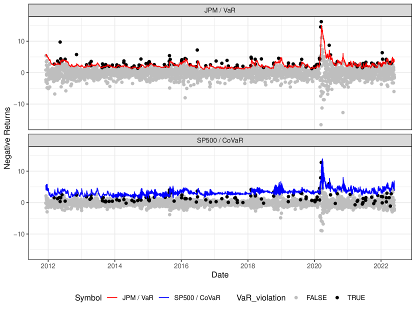
Figure 1: Out-of-sample VaR and CoVaR forecasts from the CoCAViaR-SAV-fullA model where JPMorgan Chase’s log-losses are used for $X_{t}$ and the S&P 500 for $Y_{t}$. Log-losses on days with a VaR exceedance of JPMorgan Chase are displayed in black in both panels.

Figure 1 illustrates the rolling window forecasts from the SAV-fullA CoCAViaR model for the evaluation window ranging from December 6, 2011 until December 31, 2021. The upper panel shows the log-losses of JPMorgan Chase—the systemically most important bank according to the Financial Stability Board (2021)—together with its VaR forecasts. Losses exceeding the VaR forecasts are highlighted in black, which correspond to days with an (out-of-sample) stress event $\big{\{}X_{t}\geq\widehat{\operatorname{VaR}}_{t,\beta}\big{\}}$ in the definition of the CoVaR in Section 2.1. The lower panel shows the log-losses of the S&P 500 together with the model’s CoVaR forecasts. There, the log-losses of days with a VaR exceedance (of JPMorgan Chase) are displayed in black, such that the CoVaR forecasts can be interpreted as $\alpha=95\%$ quantile forecasts among these days with VaR exceedances.

As competitors for our six CoCAViaR models, we use six different DCC–GARCH specifications. DCC–GARCH models have attained benchmark status, because of their accurate variance-covariance matrix predictions (Laurent et al., 2012; Caporin and McAleer, 2014). Particularly, we use three DCC–GARCH model specifications, containing two standard DCC–GARCH(1,1) models with multivariate Gaussian and $t$-distributed innovations respectively and a DCC specification based on a univariate GJR–GARCH(1,1) model. All models are estimated by maximum likelihood. Following Section 2.5, the VaR and CoVaR forecasts are obtained by combining all three model specifications with a symmetric and a Cholesky decomposition of the forecasted variance-covariance matrices, yielding six sets of forecasts. We refer to Supplement H for details on the CoVaR computations.

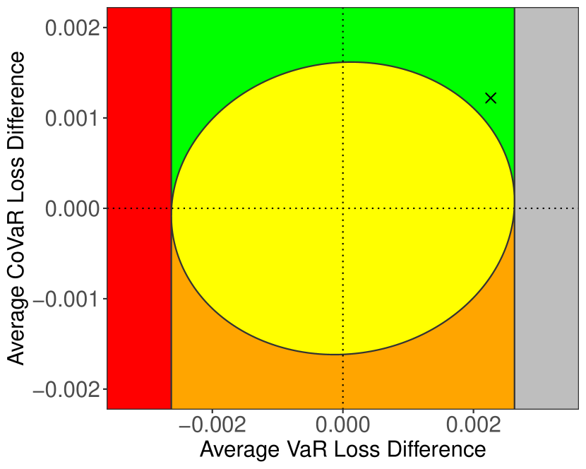
(a) CoCAViaR-SAV-fullA model

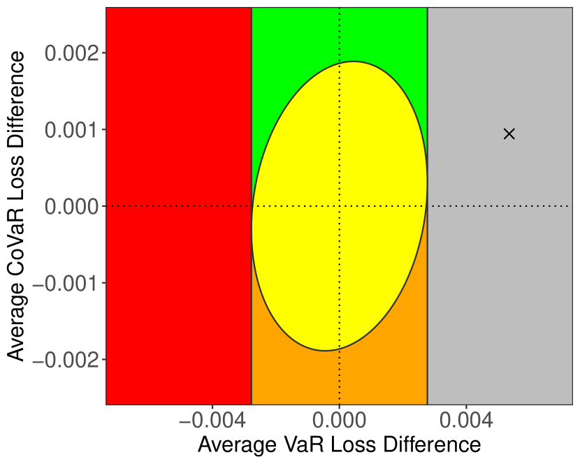
(b) CoCAViaR-AS-mixed model

Figure 2: This figure graphically illustrates the one and a half-sided forecast comparison tests for the VaR and CoVaR of Fissler and Hoga (2022) based on their multi-objective scoring function in (5) for a significance level of $10\%$. We use log-losses of JPMorgan Chase for $X_{t}$ and of the S&P 500 for $Y_{t}$. The respective CoCAViaR models are given in the captions of the two plots and are compared against the baseline “DCC-t-Chol” model.

The multi-objective elicitability of (VaR, CoVaR) complicates inference on the predictive ability of forecasts, since the scoring function in (5) is bivariate such that standard Diebold and Mariano (1995) tests—based on scalar scores—cannot be applied. We follow Fissler and Hoga (2022) and their “one and a half-sided” tests together with their extended traffic light system that we illustrate exemplarily in Figure 2 for two models. These tests require to fix a baseline model, and we arbitrarily choose the “DCC-t-Chol” model for all evaluations. Such a baseline model is necessary as classical extensions to multi-model forecast comparison methods as, e.g., the model confidence set of Hansen et al. (2011) are not available in the case of bivariate (multi-objective) scoring functions.

Multi-objective elicitability implies that the scores of two competing sequences of CoVaR forecasts can only be compared if their underlying VaR forecasts perform equally well. To obtain a reasonable finite-sample counterpart, Fissler and Hoga (2022) interpret this as an insignificant score difference in the standard Diebold and Mariano (1995) test for the VaR forecasts. Hence, the null that the expected VaR score differences (calculated based on the first component in (5)) are equal to zero cannot be rejected. The red zone in Figure 2 indicates that the baseline VaR is significantly superior, and the comparison model is rejected without consideration of its CoVaR forecasts. The grey zone indicates the reverse, while the three remaining zones in the intermediary corridor imply insignificant score differences of the VaR forecasts. Here, the orange zone implies that the baseline CoVaR is significantly superior (i.e., the CoVaR score differences based on the second component of (5) are smaller than zero in expectation), the green zone that the alternative model is superior and the yellow zone represents insignificant score differences. As the baseline is the “DCC-t-Chol” model, a comparison with our CoCAViaR models should ideally yield results in the green zone (which indicates superior CoVaR forecasts and comparable VaR forecasts) or in the grey zone (which implies superior VaR forecasts).

			VaR				CoVaR				Inference
$X_{t}$	model		score	rank	hits		score	rank	hits		zone	$p$-value
BAC	CoCAViaR-SAV-fullA		2.060	6	4.5		5.913	1	7.9		green	0.01
	CoCAViaR-AS-pos		2.062	7	4.9		6.793	2	6.5		yellow	0.11
	CoCAViaR-SAV-diag		2.096	12	4.7		6.977	3	7.6		yellow	0.18
	CoCAViaR-AS-mixed		2.041	1	4.9		7.019	4	6.4		grey	0.01
	CoCAViaR-AS-signs		2.043	4	5.0		7.228	5	7.1		grey	0.01
	CoCAViaR-SAV-full		2.060	6	4.5		7.609	6	8.8		yellow	0.30
	DCC-n-Chol		2.083	8	4.4		7.652	7	15.3		green	0.01
	DCC-t-Chol		2.086	10	4.6		8.109	8	14.5
	DCC-n-sym		2.084	9	4.4		8.139	9	15.3		yellow	0.95
	DCC-t-sym		2.086	11	4.6		8.460	10	16.4		yellow	0.71
	DCC-gjr-t-Chol		2.043	3	4.6		8.635	11	13.7		grey	0.00
	DCC-gjr-t-sym		2.042	2	4.6		8.869	12	11.2		grey	0.00
C	CoCAViaR-SAV-full		2.138	6	4.9		6.528	1	6.4		yellow	0.77
	CoCAViaR-SAV-diag		2.134	5	5.0		6.568	2	7.9		yellow	0.13
	CoCAViaR-AS-mixed		2.127	4	5.1		6.608	3	5.4		yellow	0.15
	CoCAViaR-SAV-fullA		2.138	6	4.9		6.689	4	6.4		yellow	0.12
	CoCAViaR-AS-pos		2.158	12	5.2		6.705	5	5.3		yellow	0.19
	CoCAViaR-AS-signs		2.126	3	5.1		6.714	6	6.2		yellow	0.11
	DCC-n-Chol		2.141	8	4.9		7.516	7	10.4		green	0.01
	DCC-t-Chol		2.146	11	4.9		7.750	8	11.2
	DCC-gjr-t-Chol		2.104	1	4.9		7.878	9	10.6		grey	0.01
	DCC-n-sym		2.141	9	5.0		8.035	10	11.8		yellow	0.42
	DCC-gjr-t-sym		2.107	2	5.2		8.331	11	10.7		grey	0.00
	DCC-t-sym		2.144	10	5.1		8.347	12	11.5		yellow	0.88
GS	CoCAViaR-SAV-fullA		1.840	4	5.0		6.069	1	9.5		green	0.01
	CoCAViaR-AS-mixed		1.818	1	5.0		6.460	2	4.0		grey	0.00
	CoCAViaR-AS-pos		1.820	2	4.9		6.572	3	7.2		grey	0.00
	CoCAViaR-AS-signs		1.838	3	5.1		6.855	4	3.9		grey	0.00
	CoCAViaR-SAV-full		1.840	4	5.0		7.313	5	12.7		green	0.05
	CoCAViaR-SAV-diag		1.879	8	4.9		7.338	6	8.1		green	0.02
	DCC-n-sym		1.888	9	4.7		8.485	7	14.3		yellow	0.14
	DCC-t-sym		1.890	10	4.9		9.081	8	13.8		yellow	0.31
	DCC-n-Chol		1.891	11	4.7		9.165	9	17.6		yellow	0.27
	DCC-gjr-t-sym		1.857	6	4.7		9.249	10	13.3		grey	0.00
	DCC-t-Chol		1.895	12	4.7		9.288	11	18.3
	DCC-gjr-t-Chol		1.857	7	4.9		9.536	12	16.0		grey	0.00
JPM	CoCAViaR-SAV-fullA		1.718	6	4.5		6.008	1	12.4		green	0.06
	CoCAViaR-AS-mixed		1.686	2	4.5		6.402	2	7.0		grey	0.00
	CoCAViaR-AS-signs		1.685	1	4.6		6.628	3	6.8		grey	0.00
	DCC-n-sym		1.735	9	3.8		6.751	4	14.4		green	0.07
	DCC-t-sym		1.741	12	3.9		6.987	5	17.2		yellow	0.50
	DCC-n-Chol		1.733	8	3.9		7.034	6	18.2		grey	0.01
	CoCAViaR-AS-pos		1.708	5	5.2		7.209	7	6.9		yellow	0.15
	DCC-t-Chol		1.741	11	4.0		7.396	8	19.8
	CoCAViaR-SAV-diag		1.737	10	4.7		7.443	9	8.5		yellow	0.98
	DCC-gjr-t-Chol		1.705	4	4.0		7.466	10	14.7		grey	0.02
	DCC-gjr-t-sym		1.704	3	4.0		7.666	11	11.9		grey	0.01
	CoCAViaR-SAV-full		1.718	6	4.5		9.250	12	14.2		yellow	0.15
SPF	CoCAViaR-SAV-fullA		1.416	12	4.5		5.488	1	9.6		green	0.09
	CoCAViaR-AS-mixed		1.389	4	4.9		5.865	2	7.2		yellow	0.26
	CoCAViaR-AS-signs		1.379	3	4.9		5.927	3	8.9		grey	0.03
	CoCAViaR-SAV-diag		1.409	10	4.7		6.078	4	7.6		yellow	0.22
	CoCAViaR-AS-pos		1.401	9	4.9		6.314	5	7.2		yellow	0.60
	DCC-n-Chol		1.395	6	4.4		6.514	6	15.3		grey	0.01
	DCC-t-Chol		1.400	8	4.4		6.830	7	17.9
	DCC-n-sym		1.394	5	4.6		6.900	8	15.4		yellow	0.15
	DCC-t-sym		1.400	7	4.7		7.207	9	17.6		yellow	0.93
	DCC-gjr-t-sym		1.354	1	4.7		7.593	10	9.2		grey	0.00
	DCC-gjr-t-Chol		1.357	2	4.8		7.613	11	11.5		grey	0.00
	CoCAViaR-SAV-full		1.416	12	4.5		10.261	12	12.2		yellow	0.14

Table 4: VaR and CoVAR forecasting results for $Y_{t}$ equaling S&P 500 losses and various choices of $X_{t}$. Details on the table columns is given in the main text.

Table 4 presents results on the forecast performance of all 12 models. For the VaR, we report the average VaR score (multiplied by 10 for better readability) using the first component of (5), its rank among the different models, and the “hits” as the percentage of days where the loss is larger than the VaR forecast, $X_{t}\geq\widehat{\operatorname{VaR}}_{t,\beta}$. For the CoVaR, we report the average CoVaR score using the second component (5) (multiplied by 1000 for better readability), the corresponding rank, and the CoVaR hits defined as the percentage of days where $Y_{t}\geq\widehat{\operatorname{CoVaR}}_{t,\alpha\mid\beta}$ among all days with a VaR hit, i.e., the $t$ where $X_{t}\geq\widehat{\operatorname{VaR}}_{t,\beta}$. The VaR forecast should ideally be exceeded with probability $1-\beta=5\%$, and on those days the CoVaR forecast should be exceeded with probability $1-\alpha=5\%$. The last two columns of Table 4 report results for the previously described one and a half-sided test of Fissler and Hoga (2022). There we use “DCC-t-Chol” as the baseline model, and report the test’s $p$-value together with the resulting zone of their extended traffic light system. For each considered asset $X_{t}$, we sort the table rows (i.e., the models) according to their CoVaR loss, as the CoVaR forecasts are of main interest in this section.

Overall, we find a superior forecasting performance of the CoCAViaR models for all five employed assets for $X_{t}$ compared to the DCC models. While the rankings of the VaR scores vary over the different assets, their superior forecasting performance is more substantial for the CoVaR. This is supported by CoVaR hits (corresponding to unconditional forecast calibration) much closer to the nominal level of $5\%$ than the DCC models, whose hit frequencies are almost all above $10\%$. While none of the CoCAViaR models are significantly outperformed by being in the red or orange zones, some significantly outperform the baseline DCC model and are located in the green and grey zones. Also notice that among the CoCAViaR models, the SAV-full specification (not covered by our framework) often performs the poorest. Therefore, our modeling framework (1) seems to be sufficiently general to capture the salient features of (systemic) risk evolution through time.

The favorable performance of our CoCAViaR models may be explained as follows. First, DCC–GARCH forecasts of CoVaR intimately rely on the somewhat arbitrary decomposition of the conditional variance-covariance matrix, which is a problem that is sidestepped by our modeling approach; see Section 2.5. Second, our CoCAViaR specifications directly model the quantities of interest (VaR and CoVaR), whereas multivariate GARCH processes model the whole predictive density. Third, our estimators are tailored to accurately capture the (VaR, CoVaR) evolution and, hence, do not place undue emphasis on center-of-the-distribution observations. In contrast, estimators of DCC–GARCH models may trade off a better fit in the body of the distribution for a worse fit in the tails.

Among the CoCAViaR models, we find a better performance of the AS than the SAV models for the VaR, but a relatively comparable performance for CoVaR forecasting. A reason for this may be that the additional VaR parameters in the AS models are estimated with more precision and, hence, the predictive content of the positive/negative parts emerges more clearly than for CoVaR, where the effective sample size is much reduced. It is further noteworthy that the SAV-full CoCAViaR model, that includes the lagged VaR in the CoVaR model equation performs relatively poorly. This might be caused by a high co-linearity of the VaR and CoVaR models, and also shows that the restriction $B_{12}=0$ which we have to impose for our two-step M-estimator is likely to be unproblematic in practice.

5 Conclusion

Our first main contribution is to propose a flexible, semiparametric approach for modeling (VaR, CoVaR). To the extent that we only model (VaR, CoVaR) and not the full predictive distribution, we ‘let the tails speak for themselves’ (DuMouchel, 1983). As we find in an empirical application on the systemic riskiness of US financial institutions, this yields models that improve upon benchmark DCC–GARCH models in terms of predictive accuracy. As a second main contribution, we propose a two-step M-estimator for the model parameters and derive its large sample properties. From an econometric perspective, our proofs are non-standard since the loss function that has to be used for the CoVaR is not only non-smooth, but also discontinuous in the VaR model (parameter).

We expect our modeling framework to have applications beyond the one considered here, for instance in predictive CoVaR regressions as in Adrian and Brunnermeier (2016). Furthermore, in macroeconomics, Adrian et al. (2019, 2022) have recently drawn attention to tail risks and their interconnections by popularizing the Growth-at-Risk, which is simply the VaR of GDP growth. Hence, the modeling approach developed in this paper could be relevant for studying interconnections of macroeconomic risks. Much like Brownlees and Souza (2021) compared the predictive accuracy of Growth-at-Risk model, our model may be used as a competitor in Co-Growth-at-Risk comparisons.

Appendix A Proof of Theorem 1

• Throughout the proof, $C>0$ denotes some large constant that may change from place to place. We prove both convergences by verifying conditions (i)–(iv) of Theorem 2.1 in Newey and McFadden (1994).

  First, we prove $\widehat{\bm{\theta}}_{n}^{v}\overset{\mathbb{P}}{\longrightarrow}\bm{\theta}_{0}^{v}$. For condition (i), we have to show that

  $$Q_{0}^{v}(\bm{\theta}^{v})=\mathbb{E}\bigg{[}\frac{1}{n}\sum_{t=1}^{n}S^{\operatorname{VaR}}\big{(}v_{t}(\bm{\theta}^{v}),X_{t}\big{)}\bigg{]}$$

  is uniquely minimized at $\bm{\theta}^{v}=\bm{\theta}_{0}^{v}$. By Assumption 1 (iii) and from Fissler and Hoga (2022, Theorem 4.4) it follows that $\mathbb{E}_{t-1}\big{[}S^{\operatorname{VaR}}\big{(}\cdot,X_{t}\big{)}\big{]}$ is uniquely minimized at $\operatorname{VaR}_{\beta}(X_{t}\mid\mathcal{F}_{t-1})$, which equals $v_{t}(\bm{\theta}_{0}^{v})$ under correct specification. By Assumptions 1 (i) and (vi), $\bm{\theta}_{0}^{v}$ is then the unique minimizer of $\mathbb{E}_{t-1}\big{[}S^{\operatorname{VaR}}\big{(}v_{t}(\cdot),X_{t}\big{)}\big{]}$. By the law of the iterated expectations (LIE) we have that

  $$\mathbb{E}\Big{[}S^{\operatorname{VaR}}\big{(}v_{t}(\bm{\theta}^{v}),X_{t}\big{)}\Big{]}=\mathbb{E}\bigg{\{}\mathbb{E}_{t-1}\Big{[}S^{\operatorname{VaR}}\big{(}v_{t}(\bm{\theta}^{v}),X_{t}\big{)}\Big{]}\bigg{\}},$$

  which implies that $\bm{\theta}_{0}^{v}$ is also the unique minimizer of $Q_{0}^{v}(\cdot)$, as desired.

  The compactness requirement of condition (ii) of Theorem 2.1 in Newey and McFadden (1994) is immediate from Assumption 1 (iv). Condition (iii), i.e., the continuity of $\bm{\theta}^{v}\mapsto Q_{0}^{v}(\bm{\theta}^{v})$, holds because for any $\bm{\theta}^{v}\in\bm{\varTheta}^{v}$,

  $$\lim_{\bm{\theta}\to\bm{\theta}^{v}}Q_{0}^{v}(\bm{\theta}) =\frac{1}{n}\sum_{t=1}^{n}\lim_{\bm{\theta}\to\bm{\theta}^{v}}\mathbb{E}\Big{[}S^{\operatorname{VaR}}\big{(}v_{t}(\bm{\theta}),X_{t}\big{)}\Big{]}$$

  $$=\frac{1}{n}\sum_{t=1}^{n}\mathbb{E}\Big{[}\lim_{\bm{\theta}\to\bm{\theta}^{v}}S^{\operatorname{VaR}}\big{(}v_{t}(\bm{\theta}),X_{t}\big{)}\Big{]}$$

  $$=\frac{1}{n}\sum_{t=1}^{n}\mathbb{E}\Big{[}S^{\operatorname{VaR}}\big{(}v_{t}(\bm{\theta}^{v}),X_{t}\big{)}\Big{]}=Q_{0}^{v}(\bm{\theta}^{v}),$$

  where the second step follows from the dominated convergence theorem (DCT), and the third step from the continuity of the map $v\mapsto S^{\operatorname{VaR}}(v,x)$ together with continuity of $v_{t}(\cdot)$ (by Assumption 1 (vi)). Thus, $\bm{\theta}^{v}\mapsto Q_{0}^{v}(\bm{\theta}^{v})$ is continuous. Note that we may apply the DCT, because $S^{\operatorname{VaR}}\big{(}v_{t}(\bm{\theta}),X_{t}\big{)}$ is dominated by

  $$\big{|}S^{\operatorname{VaR}}\big{(}v_{t}(\bm{\theta}),X_{t}\big{)}\big{|}\leq\big{|}X_{t}-v_{t}(\bm{\theta})\big{|}\leq\big{|}X_{t}\big{|}+\big{|}v_{t}(\bm{\theta})\big{|}\leq|X_{t}|+V(\mathcal{F}_{t-1}),$$

  where the final term is integrable due to Assumption 1 (ix). The ULLN required by condition (iv) follows directly from our Assumption 1 (v).

  Now, we prove $\widehat{\bm{\theta}}_{n}^{c}\overset{\mathbb{P}}{\longrightarrow}\bm{\theta}_{0}^{c}$. To this end, we again verify conditions (i)–(iv) of Theorem 2.1 in Newey and McFadden (1994). Condition (i) for

  $$Q_{0}^{c}(\bm{\theta}^{c})=\mathbb{E}\bigg{[}\frac{1}{n}\sum_{t=1}^{n}S^{\operatorname{CoVaR}}\big{(}(v_{t}(\bm{\theta}_{0}^{v}),c_{t}(\bm{\theta}^{c}))^{\prime},(X_{t},Y_{t})^{\prime}\big{)}\bigg{]}$$

  follows from similar arguments used in the proof of $\widehat{\bm{\theta}}_{n}^{v}\overset{\mathbb{P}}{\longrightarrow}\bm{\theta}_{0}^{v}$. Condition (ii) is in force, due to Assumption 1 (iv). Condition (iii), i.e., the continuity of $\bm{\theta}^{c}\mapsto Q_{0}^{c}(\bm{\theta}^{c})$, follows because for any $\bm{\theta}^{c}\in\bm{\varTheta}^{c}$,

  $$\lim_{\bm{\theta}\to\bm{\theta}^{c}}Q_{0}^{c}(\bm{\theta}) =\frac{1}{n}\sum_{t=1}^{n}\lim_{\bm{\theta}\to\bm{\theta}^{c}}\mathbb{E}\Big{[}S^{\operatorname{CoVaR}}\big{(}(v_{t}(\bm{\theta}_{0}^{v}),c_{t}(\bm{\theta}))^{\prime},(X_{t},Y_{t})^{\prime}\big{)}\Big{]}$$

  $$=\frac{1}{n}\sum_{t=1}^{n}\mathbb{E}\Big{[}\lim_{\bm{\theta}\to\bm{\theta}^{c}}S^{\operatorname{CoVaR}}\big{(}(v_{t}(\bm{\theta}_{0}^{v}),c_{t}(\bm{\theta}))^{\prime},(X_{t},Y_{t})^{\prime}\big{)}\Big{]}$$

  $$=\frac{1}{n}\sum_{t=1}^{n}\mathbb{E}\Big{[}S^{\operatorname{CoVaR}}\big{(}(v_{t}(\bm{\theta}_{0}^{v}),c_{t}(\bm{\theta}^{c}))^{\prime},(X_{t},Y_{t})^{\prime}\big{)}\Big{]}=Q_{0}^{c}(\bm{\theta}^{c}),$$

  where the second step follows from the DCT, and the third step from the continuity of the map $c\mapsto S^{\operatorname{CoVaR}}\big{(}(v,c)^{\prime},(x,y)^{\prime}\big{)}$ together with the continuity of $c_{t}(\cdot)$ (by Assumption 1 (vi)). Thus, $\bm{\theta}^{c}\mapsto Q_{0}^{c}(\bm{\theta}^{c})$ is continuous. Note that we may apply the DCT, because $S^{\operatorname{CoVaR}}\big{(}(v_{t}(\bm{\theta}_{0}^{v}),c_{t}(\bm{\theta}))^{\prime},(X_{t},Y_{t})^{\prime}\big{)}$ is dominated by

  $$\big{|}S^{\operatorname{CoVaR}}\big{(}(v_{t}(\bm{\theta}_{0}^{v}),c_{t}(\bm{\theta}))^{\prime},(X_{t},Y_{t})^{\prime}\big{)}\big{|}\leq\big{|}Y_{t}-c_{t}(\bm{\theta})\big{|}\leq\big{|}Y_{t}\big{|}+\big{|}c_{t}(\bm{\theta})\big{|}\leq|Y_{t}|+C(\mathcal{F}_{t-1}),$$

  where the final term is integrable due to Assumption 1 (ix). For condition (iv), let

  $$\widehat{Q}_{n}^{c}(\bm{\theta}^{c})=\frac{1}{n}\sum_{t=1}^{n}S^{\operatorname{CoVaR}}\big{(}(v_{t}(\widehat{\bm{\theta}}_{n}^{v}),c_{t}(\bm{\theta}^{c}))^{\prime},(X_{t},Y_{t})^{\prime}\big{)},$$

  where we absorb the fact that $\widehat{\bm{\theta}}_{n}^{v}$ is estimated into $\widehat{Q}_{n}^{c}(\cdot)$. We then have to show that

  $$\sup_{\bm{\theta}^{c}\in\bm{\varTheta}^{c}}\Big{|}\widehat{Q}_{n}^{c}(\bm{\theta}^{c})-Q_{0}^{c}(\bm{\theta}^{c})\Big{|}$$

  $$=\sup_{\bm{\theta}^{c}\in\bm{\varTheta}^{c}}\bigg{|}\frac{1}{n}\sum_{t=1}^{n}S^{\operatorname{CoVaR}}\big{(}(v_{t}(\widehat{\bm{\theta}}_{n}^{v}),c_{t}(\bm{\theta}^{c}))^{\prime},(X_{t},Y_{t})^{\prime}\big{)}-\mathbb{E}\Big{[}S^{\operatorname{CoVaR}}\big{(}(v_{t}(\bm{\theta}_{0}^{v}),c_{t}(\bm{\theta}^{c}))^{\prime},(X_{t},Y_{t})^{\prime}\big{)}\Big{]}\bigg{|}$$

  is $o_{\mathbb{P}}(1)$. The term in the second line can be bounded by

  $$A_{1n}+B_{1n}\mathrel{\mathop{\mathchar 58\relax}}=$$

  $$\sup_{\bm{\theta}^{c}\in\bm{\varTheta}^{c}}\bigg{|}\frac{1}{n}\sum_{t=1}^{n}S^{\operatorname{CoVaR}}\big{(}(v_{t}(\widehat{\bm{\theta}}_{n}^{v}),c_{t}(\bm{\theta}^{c}))^{\prime},(X_{t},Y_{t})^{\prime}\big{)}-\mathbb{E}\Big{[}S^{\operatorname{CoVaR}}\big{(}(v_{t}(\widehat{\bm{\theta}}_{n}^{v}),c_{t}(\bm{\theta}^{c}))^{\prime},(X_{t},Y_{t})^{\prime}\big{)}\Big{]}\bigg{|}$$

  $$+\sup_{\bm{\theta}^{c}\in\bm{\varTheta}^{c}}\bigg{|}\frac{1}{n}\sum_{t=1}^{n}\mathbb{E}\Big{[}S^{\operatorname{CoVaR}}\big{(}(v_{t}(\widehat{\bm{\theta}}_{n}^{v}),c_{t}(\bm{\theta}^{c}))^{\prime},(X_{t},Y_{t})^{\prime}\big{)}\Big{]}-\mathbb{E}\Big{[}S^{\operatorname{CoVaR}}\big{(}(v_{t}(\bm{\theta}_{0}^{v}),c_{t}(\bm{\theta}^{c}))^{\prime},(X_{t},Y_{t})^{\prime}\big{)}\Big{]}\bigg{|}.$$

  We show in turn that $A_{1n}=o_{\mathbb{P}}(1)$ and $B_{1n}=o_{\mathbb{P}}(1)$. By the ULLN from Assumption 1 (v) it holds that

  $$A_{1n} \leq\sup_{(\bm{\theta}^{v},\bm{\theta}^{c})^{\prime}\in\bm{\varTheta}}\bigg{|}\frac{1}{n}\sum_{t=1}^{n}S^{\operatorname{CoVaR}}\big{(}(v_{t}(\bm{\theta}^{v}),c_{t}(\bm{\theta}^{c}))^{\prime},(X_{t},Y_{t})^{\prime}\big{)}$$

  $$\hskip 113.81102pt-\mathbb{E}\Big{[}S^{\operatorname{CoVaR}}\big{(}(v_{t}(\bm{\theta}^{v}),c_{t}(\bm{\theta}^{c}))^{\prime},(X_{t},Y_{t})^{\prime}\big{)}\Big{]}\bigg{|}$$

  $$=o_{\mathbb{P}}(1).$$

It remains to show $B_{1n}=o_{\mathbb{P}}(1)$. For any $\varepsilon>0$ and $\delta>0$ (with $\delta$ chosen sufficiently small, such that Assumption 1 (viii) is satisfied) it holds that

$$\mathbb{P}\big{\{}B_{1n}>\varepsilon\big{\}} \leq\mathbb{P}\Big{\{}B_{1n}>\varepsilon,\ \big{\lVert}\widehat{\bm{\theta}}_{n}^{v}-\bm{\theta}_{0}^{v}\big{\rVert}\leq\delta\Big{\}}+\mathbb{P}\Big{\{}\big{\lVert}\widehat{\bm{\theta}}_{n}^{v}-\bm{\theta}_{0}^{v}\big{\rVert}>\delta\Big{\}}$$

$$\leq\mathbb{P}\Bigg{\{}\frac{1}{n}\sum_{t=1}^{n}\mathbb{E}\bigg{[}\sup_{\begin{subarray}{c}\bm{\theta}^{c}\in\bm{\varTheta}^{c}\\ \mathinner{\!\left\lVert\bm{\theta}^{v}-\bm{\theta}_{0}^{v}\right\rVert}\leq\delta\end{subarray}}\Big{|}S^{\operatorname{CoVaR}}\big{(}(v_{t}(\bm{\theta}^{v}),c_{t}(\bm{\theta}^{c}))^{\prime},(X_{t},Y_{t})^{\prime}\big{)}$$

$$\hskip 113.81102pt-S^{\operatorname{CoVaR}}\big{(}(v_{t}(\bm{\theta}_{0}^{v}),c_{t}(\bm{\theta}^{c}))^{\prime},(X_{t},Y_{t})^{\prime}\big{)}\Big{|}\bigg{]}>\varepsilon\Bigg{\}}+o(1).$$ (A.1)

Define the $\mathcal{F}_{t-1}$-measurable quantities

$$\underline{\bm{\tau}} \mathrel{\mathop{\mathchar 58\relax}}=\operatorname*{arg\,min}_{\|\bm{\tau}-\bm{\theta}_{0}^{v}\|\leq\delta}v_{t}(\bm{\tau}),$$

$$\overline{\bm{\tau}} \mathrel{\mathop{\mathchar 58\relax}}=\operatorname*{arg\,max}_{\|\bm{\tau}-\bm{\theta}_{0}^{v}\|\leq\delta}v_{t}(\bm{\tau}),$$

which exist by continuity of $v_{t}(\cdot)$ (see Assumption 1 (vi)). Write

$$\sup_{\begin{subarray}{c}\bm{\theta}^{c}\in\bm{\varTheta}^{c}\\ \mathinner{\!\left\lVert\bm{\theta}^{v}-\bm{\theta}_{0}^{v}\right\rVert}\leq\delta\end{subarray}} \Big{|}S^{\operatorname{CoVaR}}\big{(}(v_{t}(\bm{\theta}^{v}),c_{t}(\bm{\theta}^{c}))^{\prime},(X_{t},Y_{t})^{\prime}\big{)}-S^{\operatorname{CoVaR}}\big{(}(v_{t}(\bm{\theta}_{0}^{v}),c_{t}(\bm{\theta}^{c}))^{\prime},(X_{t},Y_{t})^{\prime}\big{)}\Big{|}$$

$$=\sup_{\begin{subarray}{c}\bm{\theta}^{c}\in\bm{\varTheta}^{c}\\ \mathinner{\!\left\lVert\bm{\theta}^{v}-\bm{\theta}_{0}^{v}\right\rVert}\leq\delta\end{subarray}}\Big{|}\big{[}\mathds{1}_{\{X_{t}>v_{t}(\bm{\theta}^{v})\}}-\mathds{1}_{\{X_{t}>v_{t}(\bm{\theta}_{0}^{v})\}}\big{]}\big{[}\mathds{1}_{\{Y_{t}\leq c_{t}(\bm{\theta}^{c})\}}-\alpha\big{]}\big{[}c_{t}(\bm{\theta}^{c})-Y_{t}\big{]}\Big{|}$$

$$\leq\big{|}\mathds{1}_{\{X_{t}>v_{t}(\overline{\bm{\tau}})\}}-\mathds{1}_{\{X_{t}>v_{t}(\underline{\bm{\tau}})\}}\big{|}\sup_{\bm{\theta}^{c}\in\bm{\varTheta}^{c}}\Big{|}\big{[}\mathds{1}_{\{Y_{t}\leq c_{t}(\bm{\theta}^{c})\}}-\alpha\big{]}\big{[}c_{t}(\bm{\theta}^{c})-Y_{t}\big{]}\Big{|}$$

$$\leq\big{|}\mathds{1}_{\{X_{t}>v_{t}(\overline{\bm{\tau}})\}}-\mathds{1}_{\{X_{t}>v_{t}(\underline{\bm{\tau}})\}}\big{|}\Big{[}\sup_{\bm{\theta}^{c}\in\bm{\varTheta}^{c}}\big{|}c_{t}(\bm{\theta}^{c})\big{|}+|Y_{t}|\Big{]}.$$

Therefore,

$$\mathbb{E}\bigg{[}\sup_{\begin{subarray}{c}\bm{\theta}^{c}\in\bm{\varTheta}^{c}\\ \mathinner{\!\left\lVert\bm{\theta}^{v}-\bm{\theta}_{0}^{v}\right\rVert}\leq\delta\end{subarray}}\Big{|}S^{\operatorname{CoVaR}}\big{(}(v_{t}(\bm{\theta}^{v}),c_{t}(\bm{\theta}^{c}))^{\prime},(X_{t},Y_{t})^{\prime}\big{)}-S^{\operatorname{CoVaR}}\big{(}(v_{t}(\bm{\theta}_{0}^{v}),c_{t}(\bm{\theta}^{c}))^{\prime},(X_{t},Y_{t})^{\prime}\big{)}\Big{|}\bigg{]}$$

$$\leq\mathbb{E}\Big{[}\big{|}\mathds{1}_{\{X_{t}>v_{t}(\overline{\bm{\tau}})\}}-\mathds{1}_{\{X_{t}>v_{t}(\underline{\bm{\tau}})\}}\big{|}\cdot\sup_{\bm{\theta}^{c}\in\bm{\varTheta}^{c}}\big{|}c_{t}(\bm{\theta}^{c})\big{|}\Big{]}+\mathbb{E}\Big{[}\big{|}\mathds{1}_{\{X_{t}>v_{t}(\overline{\bm{\tau}})\}}-\mathds{1}_{\{X_{t}>v_{t}(\underline{\bm{\tau}})\}}\big{|}\cdot\big{|}Y_{t}\big{|}\Big{]}$$

$$=\mathrel{\mathop{\mathchar 58\relax}}B_{11t}+B_{12t}.$$

For $B_{11t}$, we obtain using the LIE (in the first step), Assumption 1 (iii) (in the third step), the mean value theorem (in the fourth step) and Assumptions 1 (viii)–(ix) (in the fifth and sixth step) that

$$B_{11t} =\mathbb{E}\bigg{\{}\sup_{\bm{\theta}^{c}\in\bm{\varTheta}^{c}}\big{|}c_{t}(\bm{\theta}^{c})\big{|}\mathbb{E}_{t-1}\Big{[}\big{|}\mathds{1}_{\{X_{t}>v_{t}(\overline{\bm{\tau}})\}}-\mathds{1}_{\{X_{t}>v_{t}(\underline{\bm{\tau}})\}}\big{|}\Big{]}\bigg{\}}$$

$$\leq\mathbb{E}\bigg{\{}C(\mathcal{F}_{t-1})\Big{|}\int_{v_{t}(\underline{\bm{\tau}})}^{v_{t}(\overline{\bm{\tau}})}f_{t}^{X}(x)\,\mathrm{d}x\Big{|}\bigg{\}}$$

$$\leq\mathbb{E}\Big{\{}C(\mathcal{F}_{t-1})K\big{|}v_{t}(\overline{\bm{\tau}})-v_{t}(\underline{\bm{\tau}})\big{|}\Big{\}}$$

$$\leq K\mathbb{E}\Big{\{}C(\mathcal{F}_{t-1})\mathinner{\!\left\lVert\nabla v_{t}(\bm{\tau}^{*})\right\rVert}\cdot\mathinner{\!\left\lVert\overline{\bm{\tau}}-\underline{\bm{\tau}}\right\rVert}\Big{\}}$$

$$\leq K\mathbb{E}\Big{\{}C(\mathcal{F}_{t-1})V_{1}(\mathcal{F}_{t-1})\Big{\}}2\delta$$

$$\leq C\delta,$$

where $\bm{\tau}^{\ast}$ is some mean value between $\underline{\bm{\tau}}$ and $\overline{\bm{\tau}}$. Hence, choosing $\delta>0$ sufficiently small, we can ensure that $\sup_{\begin{subarray}{c}\bm{\theta}^{c}\in\bm{\varTheta}^{c}\\ \mathinner{\!\left\lVert\bm{\theta}^{v}-\bm{\theta}_{0}^{v}\right\rVert}\leq\delta\end{subarray}}B_{11t}<\varepsilon/2$.

For $B_{12t}$, we obtain from Hölder’s inequality that for $p=(1+\iota)/\iota$ and $q=1+\iota$,

$$B_{12t}\leq\Big{\{}\mathbb{E}\big{|}\mathds{1}_{\{X_{t}>v_{t}(\overline{\bm{\tau}})\}}-\mathds{1}_{\{X_{t}>v_{t}(\underline{\bm{\tau}})\}}\big{|}^{p}\Big{\}}^{1/p}\Big{\{}\mathbb{E}|Y_{t}|^{q}\Big{\}}^{1/q}.$$ (A.2)

By the LIE,

$$\mathbb{E}\big{|}\mathds{1}_{\{X_{t}>v_{t}(\overline{\bm{\tau}})\}}-\mathds{1}_{\{X_{t}>v_{t}(\underline{\bm{\tau}})\}}\big{|}^{p} =\mathbb{E}\Big{[}\mathbb{E}_{t-1}\big{|}\mathds{1}_{\{X_{t}>v_{t}(\overline{\bm{\tau}})\}}-\mathds{1}_{\{X_{t}>v_{t}(\underline{\bm{\tau}})\}}\big{|}^{p}\Big{]}$$

$$=\mathbb{E}\Big{[}\mathbb{E}_{t-1}\big{|}\mathds{1}_{\{X_{t}>v_{t}(\overline{\bm{\tau}})\}}-\mathds{1}_{\{X_{t}>v_{t}(\underline{\bm{\tau}})\}}\big{|}\Big{]}$$

$$=\mathbb{E}\Big{|}F_{t}^{X}\big{(}v_{t}(\overline{\bm{\tau}})\big{)}-F_{t}^{X}\big{(}v_{t}(\underline{\bm{\tau}})\big{)}\Big{|}$$

$$=\mathbb{E}\Big{[}f_{t}^{X}\big{(}v_{t}(\bm{\tau}^{\ast})\big{)}\big{|}v_{t}(\overline{\bm{\tau}})-v_{t}(\underline{\bm{\tau}})\big{|}\Big{]}$$

$$\leq\mathbb{E}\Big{[}K\big{|}v_{t}(\bm{\tau}^{\ast})[\overline{\bm{\tau}}-\underline{\bm{\tau}}\big{|}\Big{]}$$

$$\leq\mathbb{E}\Big{[}KV_{1}(\mathcal{F}_{t-1})\big{\|}\overline{\bm{\tau}}-\underline{\bm{\tau}}\big{\|}\Big{]}$$

$$\leq K\mathbb{E}\big{[}V_{1}(\mathcal{F}_{t-1})\big{]}2\delta,$$

where $\bm{\tau}^{\ast}$ (which may change from line to line) lies between $\underline{\bm{\tau}}$ and $\overline{\bm{\tau}}$, and the penultimate step follows from Assumption 1 (viii). Plugging this into (A.2) gives

$$B_{12t}\leq C\Big{\{}\mathbb{E}\big{[}V_{1}(\mathcal{F}_{t-1})\big{]}\Big{\}}^{1/p}\Big{\{}\mathbb{E}|Y_{t}|^{q}\Big{\}}^{1/q}\delta^{1/p}.$$

Now, Assumption 1 (ix) allows us to conclude that $\sup_{\begin{subarray}{c}\bm{\theta}^{c}\in\bm{\varTheta}^{c}\\ \mathinner{\!\left\lVert\bm{\theta}^{v}-\bm{\theta}_{0}^{v}\right\rVert}\leq\delta\end{subarray}}B_{12t}<\varepsilon/2$ by choosing $\delta>0$ sufficiently small. Therefore, for a suitable choice of $\delta$, the first right-hand side term in (A.1) can be shown to equal zero, such that $B_{1n}=o_{\mathbb{P}}(1)$ follows. This establishes condition (iv). The desired result that $\widehat{\bm{\theta}}_{n}^{c}\overset{\mathbb{P}}{\longrightarrow}\bm{\theta}_{0}^{c}$ now follows from Theorem 2.1 in Newey and McFadden (1994). ∎

Appendix B Proof of Theorem 2

We split the proof of Theorem 2 into two parts. In Section B.1, we prove the asymptotic normality of $\widehat{\bm{\theta}}_{n}^{v}$, and in Section B.2 that of $\widehat{\bm{\theta}}_{n}^{c}$.

B.1 Asymptotic Normality of the VaR Parameter Estimator

The proof follows closely that of Theorem 2 in Engle and Manganelli (2004), although some of our assumptions differ from theirs. Our main motivation for detailing the proof is that some of the subsequent results are needed to prove the asymptotic normality of $\widehat{\bm{\theta}}_{n}^{c}$ in Section B.2.

Before giving the formal proof, we collect some results that will be used in the sequel. For $v\neq x$, it holds that

$$\frac{\partial}{\partial v}S^{\operatorname{VaR}}(v,x)=\big{[}\mathds{1}_{\{x\leq v\}}-\beta\big{]}.$$

Thus, by the chain rule, it holds a.s. that

$$\mathsf{\mathbf{v}}_{t}(\bm{\theta}^{v})\mathrel{\mathop{\mathchar 58\relax}}=\frac{\partial}{\partial\bm{\theta}^{v}}S^{\operatorname{VaR}}(v_{t}(\bm{\theta}^{v}),X_{t})=\nabla v_{t}(\bm{\theta}^{v})\big{[}\mathds{1}_{\{X_{t}\leq v_{t}(\bm{\theta}^{v})\}}-\beta\big{]}.$$ (B.1)

Similarly as in Engle and Manganelli (2004) and Patton et al. (2019), the key step in the proof is to apply a mean value expansion and Lemma A.1 of Weiss (1991) to prove the following result.

Lemma V.1.

Suppose Assumptions 1 and 2 hold. Then, as $n\to\infty$,

$$\sqrt{n}\big{(}\widehat{\bm{\theta}}_{n}^{v}-\bm{\theta}_{0}^{v}\big{)}=\Big{[}\bm{\varLambda}^{-1}+o_{\mathbb{P}}(1)\Big{]}\bigg{[}-\frac{1}{\sqrt{n}}\sum_{t=1}^{n}\mathsf{\mathbf{v}}_{t}(\bm{\theta}_{0}^{v})+o_{\mathbb{P}}(1)\bigg{]}.$$

Lemma V.2.

Suppose Assumptions 1 and 2 hold. Then, as $n\to\infty$,

$$n^{-1/2}\sum_{t=1}^{n}\mathsf{\mathbf{v}}_{t}(\bm{\theta}_{0}^{v})\overset{d}{\longrightarrow}N(\bm{0},\bm{V}),$$

where $\bm{V}=\mathbb{E}\big{[}\mathsf{\mathbf{v}}_{t}(\bm{\theta}_{0}^{v})\mathsf{\mathbf{v}}_{t}^{\prime}(\bm{\theta}_{0}^{v})\big{]}=\beta(1-\beta)\mathbb{E}\big{[}\nabla v_{t}(\bm{\theta}_{0}^{v})\nabla^{\prime}v_{t}(\bm{\theta}_{0}^{v})\big{]}$.

The proofs of Lemmas V.1 and V.2 are in Supplement C.

• In this first part of the proof, we show asymptotic normality of $\widehat{\bm{\theta}}_{n}^{v}$. From Lemma V.1, we have the expansion

  $$\sqrt{n}\big{(}\widehat{\bm{\theta}}_{n}^{v}-\bm{\theta}_{0}^{v}\big{)}=\Big{[}\bm{\varLambda}^{-1}+o_{\mathbb{P}}(1)\Big{]}\bigg{[}-\frac{1}{\sqrt{n}}\sum_{t=1}^{n}\mathsf{\mathbf{v}}_{t}(\bm{\theta}_{0}^{v})+o_{\mathbb{P}}(1)\bigg{]}.$$

  From this, Slutzky’s theorem and Lemma V.2, we then obtain that, as $n\to\infty$,

  $$\sqrt{n}\big{(}\widehat{\bm{\theta}}_{n}^{v}-\bm{\theta}_{0}^{v}\big{)}\overset{d}{\longrightarrow}N\big{(}\bm{0},\bm{\varLambda}^{-1}\bm{V}\bm{\varLambda}^{-1}\big{)},$$

  which is the claimed result for the VaR parameter estimator. ∎

B.2 Asymptotic Normality of the CoVaR Parameter Estimator

The proof of the asymptotic normality of $\widehat{\bm{\theta}}_{n}^{c}$ requires some further preliminary notation and lemmas. To see the analogy to the proof of the asymptotic normality of $\widehat{\bm{\theta}}_{n}^{v}$ clearer, we label the lemmas as Lemma C.1, C.2, etc.

For $c\neq y$, it holds that

$$\frac{\partial}{\partial c}S^{\operatorname{CoVaR}}\big{(}(v,c)^{\prime},(x,y)^{\prime}\big{)}=\mathds{1}_{\{x>v\}}\big{[}\mathds{1}_{\{y\leq c\}}-\alpha\big{]}.$$

Thus, by the chain rule, it holds a.s. that

$$\mathsf{\mathbf{c}}_{t}(\bm{\theta}^{c},\bm{\theta}^{v}) \mathrel{\mathop{\mathchar 58\relax}}=\frac{\partial}{\partial\bm{\theta}^{c}}S^{\operatorname{CoVaR}}\big{(}(v_{t}(\bm{\theta}^{v}),c_{t}(\bm{\theta}^{c}))^{\prime},(X_{t},Y_{t})^{\prime}\big{)}$$

$$=\mathds{1}_{\{X_{t}>v_{t}(\bm{\theta}^{v})\}}\nabla c_{t}(\bm{\theta}^{c})\big{[}\mathds{1}_{\{Y_{t}\leq c_{t}(\bm{\theta}^{c})\}}-\alpha\big{]}.$$ (B.2)

The crucial step in the proof is once again to apply a mean value expansion and Lemma A.1 of Weiss (1991) to prove

Lemma C.1.

Suppose Assumptions 1 and 2 hold. Then, as $n\to\infty$,

$$\sqrt{n}\big{(}\widehat{\bm{\theta}}_{n}^{c}-\bm{\theta}_{0}^{c}\big{)}=\big{[}\bm{\varLambda}_{(1)}^{-1}\bm{\varLambda}_{(2)}\bm{\varLambda}^{-1}+o_{\mathbb{P}}(1)\big{]}\bigg{[}\frac{1}{\sqrt{n}}\sum_{t=1}^{n}\mathsf{\mathbf{v}}_{t}(\bm{\theta}_{0}^{v})+o_{\mathbb{P}}(1)\bigg{]}\\ -\big{[}\bm{\varLambda}_{(1)}^{-1}+o_{\mathbb{P}}(1)\big{]}\bigg{[}\frac{1}{\sqrt{n}}\sum_{t=1}^{n}\mathsf{\mathbf{c}}_{t}(\bm{\theta}_{0,n}^{c},\widehat{\bm{\theta}}_{n}^{v})+o_{\mathbb{P}}(1)\bigg{]},$$

where $\bm{\theta}_{0,n}^{c}$ is defined in the proof of Lemma C.1.

Lemma C.2.

Suppose Assumptions 1 and 2 hold. Then, as $n\to\infty$,

$$n^{-1/2}\sum_{t=1}^{n}\mathsf{\mathbf{c}}_{t}(\bm{\theta}_{0,n}^{c},\widehat{\bm{\theta}}_{n}^{v})\overset{d}{\longrightarrow}N(\bm{0},\bm{C}^{\ast}),$$

where $\bm{C}^{\ast}=\mathbb{E}\big{[}\mathsf{\mathbf{c}}_{t}(\bm{\theta}_{0}^{c},\bm{\theta}_{0}^{v})\mathsf{\mathbf{c}}_{t}^{\prime}(\bm{\theta}_{0}^{c},\bm{\theta}_{0}^{v})\big{]}=\alpha(1-\alpha)(1-\beta)\mathbb{E}\big{[}\nabla c_{t}(\bm{\theta}_{0}^{c})\nabla^{\prime}c_{t}(\bm{\theta}_{0}^{c})\big{]}$.

The proofs of Lemmas C.1 and C.2 are in Supplement D.

• We can now show asymptotic normality of $\widehat{\bm{\theta}}_{n}^{c}$. From Lemma C.1, we have the decomposition

  $$\sqrt{n}\big{(}\widehat{\bm{\theta}}_{n}^{c}-\bm{\theta}_{0}^{c}\big{)} =\big{[}\bm{\varLambda}_{(1)}^{-1}\bm{\varLambda}_{(2)}\bm{\varLambda}^{-1}+o_{\mathbb{P}}(1)\big{]}\bigg{[}\frac{1}{\sqrt{n}}\sum_{t=1}^{n}\mathsf{\mathbf{v}}_{t}(\bm{\theta}_{0}^{v})+o_{\mathbb{P}}(1)\bigg{]}$$

  $$\hskip 170.71652pt-\big{[}\bm{\varLambda}_{(1)}^{-1}+o_{\mathbb{P}}(1)\big{]}\bigg{[}\frac{1}{\sqrt{n}}\sum_{t=1}^{n}\mathsf{\mathbf{c}}_{t}(\bm{\theta}_{0,n}^{c},\widehat{\bm{\theta}}_{n}^{v})+o_{\mathbb{P}}(1)\bigg{]}$$

  $$=\Big{(}\begin{array}[]{c|c}\bm{\varLambda}_{(1)}^{-1}\bm{\varLambda}_{(2)}\bm{\varLambda}^{-1}+o_{\mathbb{P}}(1)&-\bm{\varLambda}_{(1)}^{-1}+o_{\mathbb{P}}(1)\end{array}\Big{)}\begin{pmatrix}\frac{1}{\sqrt{n}}\sum_{t=1}^{n}\mathsf{\mathbf{v}}_{t}(\bm{\theta}_{0}^{v})+o_{\mathbb{P}}(1)\\ \frac{1}{\sqrt{n}}\sum_{t=1}^{n}\mathsf{\mathbf{c}}_{t}(\bm{\theta}_{0,n}^{c},\widehat{\bm{\theta}}_{n}^{v})+o_{\mathbb{P}}(1)\end{pmatrix}.$$

  From simple adaptations of the proofs of Lemmas V.2 and C.2, we have that, as $n\to\infty$,

  $$n^{-1/2}\sum_{t=1}^{n}\begin{pmatrix}\mathsf{\mathbf{v}}_{t}(\bm{\theta}_{0}^{v})\\ \mathsf{\mathbf{c}}_{t}(\bm{\theta}_{0,n}^{c},\widehat{\bm{\theta}}_{n}^{v})\end{pmatrix}\overset{d}{\longrightarrow}N(\bm{0},\bm{C}),$$

  where

  $$\bm{C}=\begin{pmatrix}\mathbb{E}\big{[}\mathsf{\mathbf{v}}_{t}(\bm{\theta}_{0}^{v})\mathsf{\mathbf{v}}_{t}^{\prime}(\bm{\theta}_{0}^{v})\big{]}&\mathbb{E}\big{[}\mathsf{\mathbf{v}}_{t}(\bm{\theta}_{0}^{v})\mathsf{\mathbf{c}}_{t}^{\prime}(\bm{\theta}_{0}^{c},\bm{\theta}_{0}^{v})\big{]}\\ \mathbb{E}\big{[}\mathsf{\mathbf{c}}_{t}(\bm{\theta}_{0}^{c},\bm{\theta}_{0}^{v})\mathsf{\mathbf{v}}_{t}^{\prime}(\bm{\theta}_{0}^{v})\big{]}&\mathbb{E}\big{[}\mathsf{\mathbf{c}}_{t}(\bm{\theta}_{0}^{c},\bm{\theta}_{0}^{v})\mathsf{\mathbf{c}}_{t}^{\prime}(\bm{\theta}_{0}^{c},\bm{\theta}_{0}^{v})\big{]}\end{pmatrix}=\begin{pmatrix}\bm{V}&\bm{0}\\ \bm{0}&\bm{C}^{\ast}\end{pmatrix}$$

  is positive definite by Assumption 2 (viii). For the above display recall (B.22) and (B.40) (from Supplement C and D, respectively), and note that

  $$\mathbb{E}\big{[}\mathsf{\mathbf{c}}_{t}(\bm{\theta}_{0}^{c},\bm{\theta}_{0}^{v})\mathsf{\mathbf{v}}_{t}^{\prime}(\bm{\theta}_{0}^{v})\big{]} =\mathbb{E}\Big{[}\nabla c_{t}(\bm{\theta}_{0}^{c})\nabla^{\prime}v_{t}(\bm{\theta}_{0}^{v})\mathds{1}_{\{X_{t}>v_{t}(\bm{\theta}_{0}^{v})\}}\big{(}\mathds{1}_{\{X_{t}\leq v_{t}(\bm{\theta}_{0}^{v})\}}-\beta\big{)}\big{(}\mathds{1}_{\{Y_{t}\leq c_{t}(\bm{\theta}_{0}^{v})\}}-\alpha\big{)}\Big{]}$$

  $$=-\beta\mathbb{E}\bigg{\{}\nabla c_{t}(\bm{\theta}_{0}^{c})\nabla^{\prime}v_{t}(\bm{\theta}_{0}^{v})\mathbb{E}_{t-1}\Big{[}\mathds{1}_{\{X_{t}>v_{t}(\bm{\theta}_{0}^{v})\}}\big{(}\mathds{1}_{\{Y_{t}\leq c_{t}(\bm{\theta}_{0}^{v})\}}-\alpha\big{)}\Big{]}\bigg{\}}$$

  $$=-\beta\mathbb{E}\bigg{\{}\nabla c_{t}(\bm{\theta}_{0}^{c})\nabla^{\prime}v_{t}(\bm{\theta}_{0}^{v})\Big{[}\mathbb{P}_{t-1}\big{\{}X_{t}>v_{t}(\bm{\theta}_{0}^{v}),\ Y_{t}\leq c_{t}(\bm{\theta}_{0}^{v})\big{\}}-\alpha(1-\beta)\Big{]}\bigg{\}}$$

  $$=-\beta\mathbb{E}\bigg{\{}\nabla c_{t}(\bm{\theta}_{0}^{c})\nabla^{\prime}v_{t}(\bm{\theta}_{0}^{v})\Big{[}\mathbb{P}_{t-1}\big{\{}Y_{t}\leq c_{t}(\bm{\theta}_{0}^{v})\mid X_{t}>v_{t}(\bm{\theta}_{0}^{v})\big{\}}(1-\beta)-\alpha(1-\beta)\Big{]}\bigg{\}}$$

  $$=-\beta\mathbb{E}\bigg{\{}\nabla c_{t}(\bm{\theta}_{0}^{c})\nabla^{\prime}v_{t}(\bm{\theta}_{0}^{v})\Big{[}\alpha(1-\beta)-\alpha(1-\beta)\Big{]}\bigg{\}}=\bm{0}$$

  and, similarly, $\mathbb{E}\big{[}\mathsf{\mathbf{v}}_{t}(\bm{\theta}_{0}^{v})\mathsf{\mathbf{c}}_{t}^{\prime}(\bm{\theta}_{0}^{c},\bm{\theta}_{0}^{v})\big{]}=\bm{0}$. We then obtain from the continuous mapping theorem that, as $n\to\infty$,

  $$\sqrt{n}\big{(}\widehat{\bm{\theta}}_{n}^{c}-\bm{\theta}_{0}^{c}\big{)}\overset{d}{\longrightarrow}N(\bm{0},\bm{\varGamma}\bm{C}\bm{\varGamma}^{\prime}),$$

  where

  $$\bm{\varGamma}=\Big{(}\begin{array}[]{c|c}\bm{\varLambda}_{(1)}^{-1}\bm{\varLambda}_{(2)}\bm{\varLambda}^{-1}&-\bm{\varLambda}_{(1)}^{-1}\end{array}\Big{)}.$$

  This, however, is just the conclusion. ∎

Supplementary Material for
Dynamic CoVaR Modeling
Timo Dimitriadis and Yannick Hoga

Continuing the labeling of Sections A and B in the Appendix of the main paper, this supplement contains Sections C–H. Specifically, Section C proves Lemmas V.1 and V.2, while Section D contains the proofs of Lemmas C.1 and C.2. Section E establishes Theorem 3. Section F shows consistency of our estimator under arbitrary starting values. In Section G, we verify Assumptions 1 and 2 for a CCC–GARCH model. We also give some details on the computation of VaR and CoVaR from DCC–GARCH models in Section H. A joint reference list is given at the end of the main paper.

Notation

We use the following notational conventions throughout this appendix. The probability space that we work on is $\big{(}\Omega,\mathcal{F},\mathbb{P}\big{)}$. We denote by $C>0$ a large positive constant that may change from line to line. If not specified otherwise, all convergences are to be understood with respect to $n\to\infty$. We also write $\mathbb{E}_{t-1}[\cdot]=\mathbb{E}[\cdot\mid\mathcal{F}_{t-1}]$ and $\mathbb{P}_{t-1}\{\cdot\}=\mathbb{P}\{\cdot\mid\mathcal{F}_{t-1}\}$ for short. We exploit without further mention that the Frobenius norm is submultiplicative, i.e., that $\mathinner{\!\left\lVert\bm{A}\bm{B}\right\rVert}\leq\mathinner{\!\left\lVert\bm{A}\right\rVert}\cdot\mathinner{\!\left\lVert\bm{B}\right\rVert}$ for conformable matrices $\bm{A}$ and $\bm{B}$. For a real-valued, differentiable function $f(\cdot)$, we denote the $j$-th element of the gradient $\nabla f(\cdot)$ by $\nabla_{j}f(\cdot)$.

Appendix C Proof of Lemmas V.1 and V.2

Before proving Lemmas V.1 and V.2, we introduce some convenient notation. Recall from (B.3) that

$$\mathsf{\mathbf{v}}_{t}(\bm{\theta}^{v})=\nabla v_{t}(\bm{\theta}^{v})\big{[}\mathds{1}_{\{X_{t}\leq v_{t}(\bm{\theta}^{v})\}}-\beta\big{]}.$$ (B.3)

This implies by the LIE and Assumption 1 (vi) that

$$\mathbb{E}\big{[}\mathsf{\mathbf{v}}_{t}(\bm{\theta}^{v})\big{]}=\mathbb{E}\bigg{\{}\nabla v_{t}(\bm{\theta}^{v})\Big{[}F_{t}^{X}\big{(}v_{t}(\bm{\theta}^{v})\big{)}-\beta\Big{]}\bigg{\}}.$$

Assumption 2 and the dominated convergence theorem allow us to interchange differentiation and expectation to yield that

$$\frac{\partial}{\partial\bm{\theta}^{v}}\mathbb{E}\big{[}\mathsf{\mathbf{v}}_{t}(\bm{\theta}^{v})\big{]}=\mathbb{E}\bigg{\{}\nabla^{2}v_{t}(\bm{\theta}^{v})\Big{[}F_{t}^{X}\big{(}v_{t}(\bm{\theta}^{v})\big{)}-\beta\Big{]}+\nabla v_{t}(\bm{\theta}^{v})\nabla^{\prime}v_{t}(\bm{\theta}^{v})f_{t}^{X}\big{(}v_{t}(\bm{\theta}^{v})\big{)}\bigg{\}}.$$ (B.4)

Evaluating this quantity at the true parameters gives

$$\bm{\varLambda} =\frac{\partial}{\partial\bm{\theta}^{v}}\mathbb{E}\big{[}\mathsf{\mathbf{v}}_{t}(\bm{\theta}^{v})\big{]}\Big{|}_{\bm{\theta}^{v}=\bm{\theta}_{0}^{v}}=\mathbb{E}\bigg{\{}\nabla v_{t}(\bm{\theta}_{0}^{v})\nabla^{\prime}v_{t}(\bm{\theta}_{0}^{v})f_{t}^{X}\big{(}v_{t}(\bm{\theta}_{0}^{v})\big{)}\bigg{\}}.$$ (B.5)

By virtue of Assumption 1 (ii), $\bm{\varLambda}$ does not depend on $t$. Finally, define

$$\bm{\lambda}_{n}(\bm{\theta}^{v}) =\frac{1}{n}\sum_{t=1}^{n}\mathbb{E}\big{[}\mathsf{\mathbf{v}}_{t}(\bm{\theta}^{v})\big{]},$$

$$\bm{\varLambda}_{n}(\bm{\theta}^{\ast}) =\frac{1}{n}\sum_{t=1}^{n}\frac{\partial}{\partial\bm{\theta}^{v}}\mathbb{E}\big{[}\mathsf{\mathbf{v}}_{t}(\bm{\theta}^{v})\big{]}\Big{|}_{\bm{\theta}^{v}=\bm{\theta}^{\ast}},$$

and note that $\bm{\varLambda}=\bm{\varLambda}_{n}(\bm{\theta}_{0}^{v})$.

• The mean value theorem (MVT) implies that for all $i=1,\ldots,p$,

  $$\lambda_{n}^{(i)}(\widehat{\bm{\theta}}_{n}^{v})=\lambda_{n}^{(i)}(\bm{\theta}_{0}^{v})+\bm{\varLambda}_{n}^{(i,\cdot)}(\bm{\theta}^{\ast}_{i})(\widehat{\bm{\theta}}_{n}^{v}-\bm{\theta}_{0}^{v}),$$

  where $\bm{\lambda}_{n}(\cdot)=\big{(}\lambda_{n}^{(1)}(\cdot),\ldots,\lambda_{n}^{(p)}(\cdot)\big{)}^{\prime}$, $\bm{\varLambda}_{n}^{(i,\cdot)}(\cdot)$ denotes the $i$-th row of $\bm{\varLambda}_{n}(\cdot)$ and $\bm{\theta}^{\ast}_{i}$ lies on the line connecting $\bm{\theta}_{0}^{v}$ and $\widehat{\bm{\theta}}_{n}^{v}$. To economize on notation, we shall slightly abuse notation (here and elsewhere) by writing this as

  $$\bm{\lambda}_{n}(\widehat{\bm{\theta}}_{n}^{v})=\bm{\lambda}_{n}(\bm{\theta}_{0}^{v})+\bm{\varLambda}_{n}(\bm{\theta}^{\ast})(\widehat{\bm{\theta}}_{n}^{v}-\bm{\theta}_{0}^{v})$$ (B.6)

  for some $\bm{\theta}^{\ast}$ between $\widehat{\bm{\theta}}_{n}^{v}$ and $\bm{\theta}_{0}^{v}$; keeping in mind that the value of $\bm{\theta}^{\ast}$ is in fact different from row to row in $\bm{\varLambda}_{n}(\bm{\theta}^{\ast})$. However, this does not change any of the subsequent arguments. Interpreted verbatim, (B.6) would be an instance of what Feng et al. (2013) call the non-existent mean value theorem, which is widely applied in statistics; e.g., by Engle and Manganelli (2004) and Patton et al. (2019).

  We have that

  $$\bm{\lambda}_{n}(\bm{\theta}_{0}^{v})=\frac{1}{n}\sum_{t=1}^{n}\mathbb{E}\bigg{\{}\nabla v_{t}(\bm{\theta}_{0}^{v})\Big{[}F_{t}^{X}\big{(}v_{t}(\bm{\theta}_{0}^{v})\big{)}-\beta\Big{]}\bigg{\}}=\bm{0},$$ (B.7)

  since $F_{t}^{X}\big{(}v_{t}(\bm{\theta}_{0}^{v})\big{)}=\beta$ by correct specification. Plugging this into (B.6) gives

  $$\bm{\lambda}_{n}(\widehat{\bm{\theta}}_{n}^{v})=\bm{\varLambda}_{n}(\bm{\theta}^{\ast})(\widehat{\bm{\theta}}_{n}^{v}-\bm{\theta}_{0}^{v}).$$

  To establish the claim, we therefore only have to show that

  1. $\bm{\varLambda}_{n}^{-1}(\bm{\theta}^{\ast})=\bm{\varLambda}^{-1}+o_{\mathbb{P}}(1)$;

  2. $\sqrt{n}\bm{\lambda}_{n}(\widehat{\bm{\theta}}_{n}^{v})=-\frac{1}{\sqrt{n}}\sum_{t=1}^{n}\mathsf{\mathbf{v}}_{t}(\bm{\theta}_{0}^{v})+o_{\mathbb{P}}(1)$.

Claim (i) is verified in Lemma V.3. For this, note that since $\bm{\theta}^{\ast}$ is a mean value between $\widehat{\bm{\theta}}_{n}^{v}$ and $\bm{\theta}_{0}^{v}$, and $\widehat{\bm{\theta}}_{n}^{v}\overset{\mathbb{P}}{\longrightarrow}\bm{\theta}_{0}^{v}$ (from Theorem 1), it also follows that $\bm{\theta}^{\ast}\overset{\mathbb{P}}{\longrightarrow}\bm{\theta}_{0}^{v}$.

To prove (ii), by Lemma A.1 in Weiss (1991), we only have to show that

1. conditions (N1)–(N5) in the notation of Weiss (1991) hold;

2. $\frac{1}{\sqrt{n}}\sum_{t=1}^{n}\mathsf{\mathbf{v}}_{t}(\widehat{\bm{\theta}}_{n}^{v})=o_{\mathbb{P}}(1)$;

3. $\widehat{\bm{\theta}}_{n}^{v}\overset{\mathbb{P}}{\longrightarrow}\bm{\theta}_{0}^{v}$.

For (ii.a), note that (N1) is immediate and (N2) follows from (B.7). The mixing condition (N5) is implied by our Assumption 2 (x). Condition (N3) is verified in Lemmas V.5–V.7 below and the remaining condition (N4) in Lemma V.8. The result in (ii.b) follows from Lemma V.4 and (ii.c) follows from Theorem 1. In sum, the desired result follows. ∎

Lemma V.3.

Suppose Assumptions 1 and 2 hold. Then, as $n\to\infty$, $\bm{\varLambda}_{n}^{-1}(\bm{\theta}^{\ast})\overset{\mathbb{P}}{\longrightarrow}\bm{\varLambda}^{-1}$ for any $\bm{\theta}^{\ast}$ with $\bm{\theta}^{\ast}\overset{\mathbb{P}}{\longrightarrow}\bm{\theta}_{0}^{v}$.

• We first show that $\mathinner{\!\left\lVert\bm{\varLambda}_{n}(\bm{\tau})-\bm{\varLambda}_{n}(\bm{\theta})\right\rVert}\leq C\mathinner{\!\left\lVert\bm{\tau}-\bm{\theta}\right\rVert}$ for all $\bm{\tau},\bm{\theta}\in\mathcal{N}(\bm{\theta}_{0}^{v})$, where $\mathcal{N}(\bm{\theta}_{0}^{v})$ is some neighborhood of $\bm{\theta}_{0}^{v}$ such that Assumptions 1 (viii) and 2 (iii) holds.

Use (B.4) to write

$$\mathinner{\!\left\lVert\bm{\varLambda}_{n}(\bm{\tau})-\bm{\varLambda}_{n}(\bm{\theta})\right\rVert} =\Bigg{\|}\frac{1}{n}\sum_{t=1}^{n}\mathbb{E}\bigg{\{}\nabla^{2}v_{t}(\bm{\tau})\Big{[}F_{t}^{X}\big{(}v_{t}(\bm{\tau})\big{)}-\beta\Big{]}-\nabla^{2}v_{t}(\bm{\theta})\Big{[}F_{t}^{X}\big{(}v_{t}(\bm{\theta})\big{)}-\beta\Big{]}$$

$$\hskip 56.9055pt+\nabla v_{t}(\bm{\tau})\nabla^{\prime}v_{t}(\bm{\tau})f_{t}^{X}\big{(}v_{t}(\bm{\tau})\big{)}-\nabla v_{t}(\bm{\theta})\nabla^{\prime}v_{t}(\bm{\theta})f_{t}^{X}\big{(}v_{t}(\bm{\theta})\big{)}\bigg{\}}\Bigg{\|}$$

$$\leq\frac{1}{n}\sum_{t=1}^{n}\mathbb{E}\Big{\|}\nabla^{2}v_{t}(\bm{\tau})\Big{[}F_{t}^{X}\big{(}v_{t}(\bm{\tau})\big{)}-F_{t}^{X}\big{(}v_{t}(\bm{\theta})\big{)}\Big{]}\Big{\|}+\beta\mathbb{E}\Big{\|}\nabla^{2}v_{t}(\bm{\tau})-\nabla^{2}v_{t}(\bm{\theta})\Big{\|}$$

$$\hskip 56.9055pt+\mathbb{E}\Big{\|}\nabla v_{t}(\bm{\tau})\nabla^{\prime}v_{t}(\bm{\tau})f_{t}^{X}\big{(}v_{t}(\bm{\tau})\big{)}-\nabla v_{t}(\bm{\theta})\nabla^{\prime}v_{t}(\bm{\theta})f_{t}^{X}\big{(}v_{t}(\bm{\theta})\big{)}\Big{\|}.$$ (B.8)

By Assumption 2 (iii), we have that

$$\beta\mathbb{E}\Big{\|}\nabla^{2}v_{t}(\bm{\tau})-\nabla^{2}v_{t}(\bm{\theta})\Big{\|}\leq\beta\mathbb{E}\big{[}V_{3}(\mathcal{F}_{t-1})\big{]}\mathinner{\!\left\lVert\bm{\tau}-\bm{\theta}\right\rVert}\leq C\mathinner{\!\left\lVert\bm{\tau}-\bm{\theta}\right\rVert}.$$ (B.9)

The other two terms in (B.8) can be dealt with as follows. First, using a mean value expansion around $\bm{\theta}_{0}^{v}$ and Assumption 2, we obtain that

$$\mathbb{E}\mathinner{\!\left\lVert\nabla^{2}v_{t}(\bm{\tau})\big{[}F_{t}^{X}\big{(}v_{t}(\bm{\tau})\big{)}-F_{t}^{X}\big{(}v_{t}(\bm{\theta})\big{)}\big{]}\right\rVert} \leq\mathbb{E}\mathinner{\!\left\lVert V_{2}(\mathcal{F}_{t-1})f_{t}^{X}\big{(}v_{t}(\bm{\theta}^{\ast})\big{)}\nabla v_{t}(\bm{\theta}^{\ast})(\bm{\tau}-\bm{\theta})\right\rVert}$$

$$\leq K\mathbb{E}\big{[}V_{1}(\mathcal{F}_{t-1})V_{2}(\mathcal{F}_{t-1})\big{]}\mathinner{\!\left\lVert\bm{\tau}-\bm{\theta}\right\rVert}$$

$$\leq K\Big{\{}\mathbb{E}\big{[}V_{1}^{3}(\mathcal{F}_{t-1})\big{]}\Big{\}}^{1/3}\Big{\{}\mathbb{E}\big{[}V_{2}^{3/2}(\mathcal{F}_{t-1})\big{]}\Big{\}}^{2/3}\mathinner{\!\left\lVert\bm{\tau}-\bm{\theta}\right\rVert}$$

$$\leq C\mathinner{\!\left\lVert\bm{\tau}-\bm{\theta}\right\rVert},$$ (B.10)

where $\bm{\theta}^{\ast}$ is some value on the line connecting $\bm{\tau}$ and $\bm{\theta}$, and the penultimate step uses Hölder’s inequality.

Second, using a mean value expansion around $\bm{\theta}$ to obtain for some $\bm{\theta}^{\ast}$ between $\bm{\tau}$ and $\bm{\theta}$ (where $\bm{\theta}^{\ast}$ may vary from line to line) that

$$\mathbb{E}\mathinner{\!\left\lVert\nabla v_{t}(\bm{\tau})\nabla^{\prime}v_{t}(\bm{\tau})f_{t}^{X}\big{(}v_{t}(\bm{\tau})\big{)}-\nabla v_{t}(\bm{\theta})\nabla^{\prime}v_{t}(\bm{\theta})f_{t}^{X}\big{(}v_{t}(\bm{\theta})\big{)}\right\rVert}$$

$$=\bigg{\|}\mathbb{E}\Big{[}\nabla v_{t}(\bm{\tau})\nabla^{\prime}v_{t}(\bm{\tau})f_{t}^{X}\big{(}v_{t}(\bm{\tau})\big{)}-\nabla v_{t}(\bm{\theta})\nabla^{\prime}v_{t}(\bm{\tau})f_{t}^{X}\big{(}v_{t}(\bm{\tau})\big{)}$$

$$\hskip 51.21504pt+\nabla v_{t}(\bm{\theta})\nabla^{\prime}v_{t}(\bm{\tau})f_{t}^{X}\big{(}v_{t}(\bm{\tau})\big{)}-\nabla v_{t}(\bm{\theta})\nabla^{\prime}v_{t}(\bm{\theta})f_{t}^{X}\big{(}v_{t}(\bm{\tau})\big{)}$$

$$\hskip 51.21504pt+\nabla v_{t}(\bm{\theta})\nabla^{\prime}v_{t}(\bm{\theta})f_{t}^{X}\big{(}v_{t}(\bm{\tau})\big{)}-\nabla v_{t}(\bm{\theta})\nabla^{\prime}v_{t}(\bm{\theta})f_{t}^{X}\big{(}v_{t}(\bm{\theta})\big{)}\Big{]}\bigg{\|}$$

$$=\bigg{\|}\mathbb{E}\Big{[}\nabla^{2}v_{t}(\bm{\theta}^{\ast})(\bm{\tau}-\bm{\theta})\nabla^{\prime}v_{t}(\bm{\tau})f_{t}^{X}\big{(}v_{t}(\bm{\tau})\big{)}$$

$$\hskip 51.21504pt+\nabla v_{t}(\bm{\theta})(\bm{\tau}-\bm{\theta})^{\prime}[\nabla^{2}v_{t}(\bm{\theta}^{\ast})]^{\prime}f_{t}^{X}\big{(}v_{t}(\bm{\tau})\big{)}$$

$$\hskip 51.21504pt+\nabla v_{t}(\bm{\theta})\nabla^{\prime}v_{t}(\bm{\theta})\big{\{}f_{t}^{X}\big{(}v_{t}(\bm{\tau})\big{)}-f_{t}^{X}\big{(}v_{t}(\bm{\theta})\big{)}\big{\}}\Big{]}\bigg{\|}$$

$$\leq\mathbb{E}\big{[}KV_{2}(\mathcal{F}_{t-1})V_{1}(\mathcal{F}_{t-1})+KV_{1}(\mathcal{F}_{t-1})V_{2}(\mathcal{F}_{t-1})+KV_{1}^{3}(\mathcal{F}_{t-1})\big{]}\mathinner{\!\left\lVert\bm{\tau}-\bm{\theta}\right\rVert}$$

$$\leq K\bigg{(}2\Big{\{}\mathbb{E}\big{[}V_{1}^{3}(\mathcal{F}_{t-1})\big{]}\Big{\}}^{1/3}\Big{\{}\mathbb{E}\big{[}V_{2}^{3/2}(\mathcal{F}_{t-1})\big{]}\Big{\}}^{2/3}+\Big{\{}\mathbb{E}\big{[}V_{1}^{3}(\mathcal{F}_{t-1})\big{]}\Big{\}}\bigg{)}\mathinner{\!\left\lVert\bm{\tau}-\bm{\theta}\right\rVert}$$

$$\leq C\mathinner{\!\left\lVert\bm{\tau}-\bm{\theta}\right\rVert},$$ (B.11)

where we used Assumption 2.

Plugging (B.9)–(B.11) into (B.8), we obtain that

$$\mathinner{\!\left\lVert\bm{\varLambda}_{n}(\bm{\tau})-\bm{\varLambda}_{n}(\bm{\theta})\right\rVert}\leq C\mathinner{\!\left\lVert\bm{\tau}-\bm{\theta}\right\rVert}.$$ (B.12)

Using this, we obtain for $\delta>0$ with $\big{\{}\mathinner{\!\left\lVert\bm{\theta}-\bm{\theta}_{0}^{v}\right\rVert}\leq\delta\big{\}}\subset\mathcal{N}(\bm{\theta}_{0}^{v})$ that

$$\mathbb{P}\Big{\{}\mathinner{\!\left\lVert\bm{\varLambda}_{n}(\bm{\theta}^{\ast})-\bm{\varLambda}\right\rVert}>\varepsilon\Big{\}} =\mathbb{P}\Big{\{}\mathinner{\!\left\lVert\bm{\varLambda}_{n}(\bm{\theta}^{\ast})-\bm{\varLambda}_{n}(\bm{\theta}_{0}^{v})\right\rVert}>\varepsilon\Big{\}}$$

$$\leq\mathbb{P}\Big{\{}\mathinner{\!\left\lVert\bm{\varLambda}_{n}(\bm{\theta}^{\ast})-\bm{\varLambda}_{n}(\bm{\theta}_{0}^{v})\right\rVert}>\varepsilon,\ \mathinner{\!\left\lVert\bm{\theta}^{\ast}-\bm{\theta}_{0}^{v}\right\rVert}\leq\delta\Big{\}}+\mathbb{P}\Big{\{}\mathinner{\!\left\lVert\bm{\theta}^{\ast}-\bm{\theta}_{0}^{v}\right\rVert}>\delta\Big{\}}$$

$$\leq\mathbb{P}\bigg{\{}\sup_{\mathinner{\!\left\lVert\bm{\theta}-\bm{\theta}_{0}^{v}\right\rVert}\leq\delta}\mathinner{\!\left\lVert\bm{\varLambda}_{n}(\bm{\theta})-\bm{\varLambda}_{n}(\bm{\theta}_{0}^{v})\right\rVert}>\varepsilon\bigg{\}}+o(1)$$

$$\leq\mathbb{P}\bigg{\{}\sup_{\mathinner{\!\left\lVert\bm{\theta}-\bm{\theta}_{0}^{v}\right\rVert}\leq\delta}C\mathinner{\!\left\lVert\bm{\theta}-\bm{\theta}_{0}^{v}\right\rVert}>\varepsilon\bigg{\}}+o(1)$$

$$=0+o(1),$$

where the final line additionally requires $\delta<\varepsilon/C$. This shows that $\bm{\varLambda}_{n}(\bm{\theta}^{\ast})\overset{\mathbb{P}}{\longrightarrow}\bm{\varLambda}$. By Assumption 2 (viii) and continuity of $\bm{\varLambda}_{n}(\cdot)$ (recall (B.12)), $\bm{\varLambda}_{n}(\bm{\theta}^{v})$ is non-singular in a neighborhood of $\bm{\theta}_{0}^{v}$. Therefore, the continuous mapping theorem (CMT) applied to $\bm{\varLambda}_{n}(\bm{\theta}^{\ast})\overset{\mathbb{P}}{\longrightarrow}\bm{\varLambda}$ implies that $\bm{\varLambda}_{n}^{-1}(\bm{\theta}^{\ast})\overset{\mathbb{P}}{\longrightarrow}\bm{\varLambda}^{-1}$, as desired.∎

Lemma V.4.

Suppose Assumptions 1 and 2 hold. Then, as $n\to\infty$,

$$\frac{1}{\sqrt{n}}\sum_{t=1}^{n}\mathsf{\mathbf{v}}_{t}(\widehat{\bm{\theta}}_{n}^{v})=o_{\mathbb{P}}(1).$$

• Recall from Assumption 1 (iv) that $\bm{\varTheta}^{v}\subset\mathbb{R}^{p}$, such that $\bm{\theta}^{v}$ is a $p$-dimensional parameter vector. Let $\bm{e}_{1},\ldots,\bm{e}_{p}$ denote the standard basis of $\mathbb{R}^{p}$. Define

  $$S_{j,n}^{\operatorname{VaR}}(a)\mathrel{\mathop{\mathchar 58\relax}}=\frac{1}{\sqrt{n}}\sum_{t=1}^{n}S^{\operatorname{VaR}}\big{(}v_{t}(\widehat{\bm{\theta}}_{n}^{v}+a\bm{e}_{j}),X_{t}\big{)},\qquad j=1,\ldots,p,$$

  where $a\in\mathbb{R}$. Let $G_{j,n}(a)$ be the right partial derivative of $S_{j,n}^{\operatorname{VaR}}(a)$, such that (see (B.3))

  $$G_{j,n}(a)=\frac{1}{\sqrt{n}}\sum_{t=1}^{n}\nabla_{j}v_{t}(\widehat{\bm{\theta}}_{n}^{v}+a\bm{e}_{j})\big{[}\mathds{1}_{\{X_{t}\leq v_{t}(\widehat{\bm{\theta}}_{n}^{v}+a\bm{e}_{j})\}}-\beta\big{]},$$

  where $\nabla_{j}v_{t}(\cdot)$ is the $j$-th component of $\nabla v_{t}(\cdot)$. Then, $G_{j,n}(0)=\lim_{\xi\downarrow 0}G_{j,n}(\xi)$ is the right partial derivative of

  $$S_{n}^{\operatorname{VaR}}(\bm{\theta}^{v})\mathrel{\mathop{\mathchar 58\relax}}=\frac{1}{\sqrt{n}}\sum_{t=1}^{n}S^{\operatorname{VaR}}\big{(}v_{t}(\bm{\theta}^{v}),X_{t}\big{)}$$

  at $\widehat{\bm{\theta}}_{n}^{v}$ in the direction $\bm{\theta}_{j}^{v}$, where $\bm{\theta}^{v}=(\bm{\theta}_{1}^{v},\ldots,\bm{\theta}_{p}^{v})^{\prime}$. Correspondingly, $\lim_{\xi\downarrow 0}G_{j,n}(-\xi)$ is the left partial derivative. Because $S_{n}^{\operatorname{VaR}}(\cdot)$ achieves its minimum at $\widehat{\bm{\theta}}_{n}^{v}$, the left derivative must be non-positive and the right derivative must be non-negative. Thus,

  $$\big{|}G_{j,n}(0)\big{|} \leq G_{j,n}(\xi)-G_{j,n}(-\xi)$$

  $$=\frac{1}{\sqrt{n}}\sum_{t=1}^{n}\nabla_{j}v_{t}(\widehat{\bm{\theta}}_{n}^{v}+\xi\bm{e}_{j})\big{[}\mathds{1}_{\{X_{t}\leq v_{t}(\widehat{\bm{\theta}}_{n}^{v}+\xi\bm{e}_{j})\}}-\beta\big{]}$$

  $$\hskip 56.9055pt-\frac{1}{\sqrt{n}}\sum_{t=1}^{n}\nabla_{j}v_{t}(\widehat{\bm{\theta}}_{n}^{v}-\xi\bm{e}_{j})\big{[}\mathds{1}_{\{X_{t}\leq v_{t}(\widehat{\bm{\theta}}_{n}^{v}-\xi\bm{e}_{j})\}}-\beta\big{]}.$$

  By continuity of $\nabla v_{t}(\cdot)$ (see Assumption 2 (ii)) it follows upon letting $\xi\to 0$ that

  $$\big{|}G_{j,n}(0)\big{|} \leq\frac{1}{\sqrt{n}}\sum_{t=1}^{n}\big{|}\nabla_{j}v_{t}(\widehat{\bm{\theta}}_{n}^{v})\big{|}\mathds{1}_{\{X_{t}=v_{t}(\widehat{\bm{\theta}}_{n}^{v})\}}$$

  $$\leq\frac{1}{\sqrt{n}}\Big{[}\max_{t=1,\ldots,n}V_{1}(\mathcal{F}_{t-1})\Big{]}\sum_{t=1}^{n}\mathds{1}_{\{X_{t}=v_{t}(\widehat{\bm{\theta}}_{n}^{v})\}}.$$ (B.13)

  We have that, by subadditivity, Markov’s inequality and Assumption 2 (v),

  $$\mathbb{P}\Big{\{}n^{-1/2}\max_{t=1,\ldots,n}V_{1}(\mathcal{F}_{t-1})>\varepsilon\Big{\}} \leq\sum_{t=1}^{n}\mathbb{P}\Big{\{}V_{1}(\mathcal{F}_{t-1})>\varepsilon n^{1/2}\Big{\}}$$

  $$\leq\sum_{t=1}^{n}\varepsilon^{-3}n^{-3/2}\mathbb{E}\big{[}V_{1}^{3}(\mathcal{F}_{t-1})\big{]}$$

  $$=O(n^{-1/2})=o(1).$$

  Combining this with Assumption 2 (ix), we obtain from (B.13) that

  $$\big{|}G_{j,n}(0)\big{|}\overset{\text{a.s.}}{=}o_{\mathbb{P}}(1)O(1)=o_{\mathbb{P}}(1).$$

  As this holds for every $j=1,\ldots,p$, we get that

  $$\frac{1}{\sqrt{n}}\sum_{t=1}^{n}\mathsf{\mathbf{v}}_{t}(\widehat{\bm{\theta}}_{n}^{v})=\frac{1}{\sqrt{n}}\sum_{t=1}^{n}\nabla v_{t}(\widehat{\bm{\theta}}_{n}^{v})\big{[}\mathds{1}_{\{X_{t}\leq v_{t}(\widehat{\bm{\theta}}_{n}^{v})\}}-\beta\big{]}=o_{\mathbb{P}}(1),$$

  which is just the conclusion. ∎

Lemma V.5.

Suppose Assumptions 1 and 2 hold. Then, condition (N3) (i) of Weiss (1991) holds, i.e.,

$$\mathinner{\!\left\lVert\bm{\lambda}_{n}(\bm{\theta})\right\rVert}\geq a\mathinner{\!\left\lVert\bm{\theta}-\bm{\theta}_{0}^{v}\right\rVert}\qquad\text{for}\ \mathinner{\!\left\lVert\bm{\theta}-\bm{\theta}_{0}^{v}\right\rVert}\leq d_{0}$$

for sufficiently large $n$ and some $a>0$ and $d_{0}>0$.

• Choose $d_{0}>0$ sufficiently small, such that $\big{\{}\bm{\theta}\in\bm{\varTheta}^{v}\mathrel{\mathop{\mathchar 58\relax}}\ \mathinner{\!\left\lVert\bm{\theta}-\bm{\theta}_{0}^{v}\right\rVert}<d_{0}\big{\}}$ is a subset of the neighborhoods of Assumptions 1 (viii) and 2 (iii). The MVT and (B.7) imply that

  $$\bm{\lambda}_{n}(\bm{\theta}) =\bm{\lambda}_{n}(\bm{\theta}_{0}^{v})+\bm{\varLambda}_{n}(\bm{\theta}^{\ast})(\bm{\theta}-\bm{\theta}_{0}^{v})$$

  $$=\bm{\varLambda}_{n}(\bm{\theta}^{\ast})(\bm{\theta}-\bm{\theta}_{0}^{v})$$

  for some $\bm{\theta}^{\ast}$ between $\bm{\theta}$ and $\bm{\theta}_{0}^{v}$. (Again, to be precise we should allow for the mean value $\bm{\theta}^{\ast}$ to vary across rows of $\bm{\varLambda}_{n}(\bm{\theta}^{\ast})$; however, for the subsequent argument this does not matter.) Use (B.4) to write

  $$\bm{\varLambda}_{n}(\bm{\theta}^{\ast})=\frac{1}{n}\sum_{t=1}^{n}\mathbb{E}\bigg{\{}\nabla^{2}v_{t}(\bm{\theta}^{\ast})\Big{[}F_{t}^{X}\big{(}v_{t}(\bm{\theta}^{\ast})\big{)}-\beta\Big{]}+\nabla v_{t}(\bm{\theta}^{\ast})\nabla^{\prime}v_{t}(\bm{\theta}^{\ast})f_{t}^{X}\big{(}v_{t}(\bm{\theta}^{\ast})\big{)}\bigg{\}}.$$

  Recall that

  $$\bm{\varLambda}=\bm{\varLambda}_{n}(\bm{\theta}_{0}^{v})=\frac{1}{n}\sum_{t=1}^{n}\mathbb{E}\Big{[}\nabla v_{t}(\bm{\theta}_{0}^{v})\nabla^{\prime}v_{t}(\bm{\theta}_{0}^{v})f_{t}^{X}\big{(}v_{t}(\bm{\theta}_{0}^{v})\big{)}\Big{]}.$$

  We first show that

  $$\bm{\varLambda}_{n}(\bm{\theta}^{\ast})=\bm{\varLambda}+O\big{(}\mathinner{\!\left\lVert\bm{\theta}^{\ast}-\bm{\theta}_{0}^{v}\right\rVert}\big{)}$$

  by decomposing $\mathinner{\!\left\lVert\bm{\varLambda}_{n}(\bm{\theta}^{\ast})-\bm{\varLambda}\right\rVert}$ into two terms, each bounded by a $O\big{(}\mathinner{\!\left\lVert\bm{\theta}^{\ast}-\bm{\theta}_{0}^{v}\right\rVert}\big{)}$-term. We have the following decomposition:

  $$\mathinner{\!\left\lVert\bm{\varLambda}_{n}(\bm{\theta}^{\ast})-\bm{\varLambda}\right\rVert} =\bigg{\|}\frac{1}{n}\sum_{t=1}^{n}\mathbb{E}\Big{\{}\nabla^{2}v_{t}(\bm{\theta}^{\ast})\big{[}F_{t}^{X}\big{(}v_{t}(\bm{\theta}^{\ast})\big{)}-\beta\big{]}\Big{\}}$$

  $$\hskip 56.9055pt+\mathbb{E}\Big{[}\nabla v_{t}(\bm{\theta}^{\ast})\nabla^{\prime}v_{t}(\bm{\theta}^{\ast})f_{t}^{X}\big{(}v_{t}(\bm{\theta}^{\ast})\big{)}-\nabla v_{t}(\bm{\theta}_{0}^{v})\nabla^{\prime}v_{t}(\bm{\theta}_{0}^{v})f_{t}^{X}\big{(}v_{t}(\bm{\theta}_{0}^{v})\big{)}\Big{]}\bigg{\|}.$$

  First term: Following similar steps as for (B.10), we obtain that

  $$\mathinner{\!\left\lVert\mathbb{E}\Big{\{}\nabla^{2}v_{t}(\bm{\theta}^{\ast})\big{[}F_{t}^{X}\big{(}v_{t}(\bm{\theta}^{\ast})\big{)}-\beta\big{]}\Big{\}}\right\rVert}\leq C\mathinner{\!\left\lVert\bm{\theta}^{\ast}-\bm{\theta}_{0}^{v}\right\rVert}.$$

Second term: Again following similar steps as for (B.11), we get that

$$\mathinner{\!\left\lVert\frac{1}{n}\sum_{t=1}^{n}\mathbb{E}\Big{[}\nabla v_{t}(\bm{\theta}^{\ast})\nabla^{\prime}v_{t}(\bm{\theta}^{\ast})f_{t}^{X}\big{(}v_{t}(\bm{\theta}^{\ast})\big{)}-\nabla v_{t}(\bm{\theta}_{0}^{v})\nabla^{\prime}v_{t}(\bm{\theta}_{0}^{v})f_{t}^{X}\big{(}v_{t}(\bm{\theta}_{0}^{v})\big{)}\Big{]}\right\rVert}$$

$$\leq\frac{1}{n}\sum_{t=1}^{n}\mathbb{E}\mathinner{\!\left\lVert\nabla v_{t}(\bm{\theta}^{\ast})\nabla^{\prime}v_{t}(\bm{\theta}^{\ast})f_{t}^{X}\big{(}v_{t}(\bm{\theta}^{\ast})\big{)}-\nabla v_{t}(\bm{\theta}_{0}^{v})\nabla^{\prime}v_{t}(\bm{\theta}_{0}^{v})f_{t}^{X}\big{(}v_{t}(\bm{\theta}_{0}^{v})\big{)}\right\rVert}$$

$$\leq C\mathinner{\!\left\lVert\bm{\theta}^{\ast}-\bm{\theta}_{0}^{v}\right\rVert}.$$

Thus, we have shown that $\mathinner{\!\left\lVert\bm{\varLambda}_{n}(\bm{\theta}^{\ast})-\bm{\varLambda}\right\rVert}\leq C\mathinner{\!\left\lVert\bm{\theta}^{\ast}-\bm{\theta}_{0}^{v}\right\rVert}$ for some $C>0$ large enough. By Assumption 2 (viii), $\bm{\varLambda}$ has eigenvalues bounded below by some constant $a>0$. Therefore,

$$\mathinner{\!\left\lVert\bm{\lambda}_{n}(\bm{\theta})\right\rVert} =\mathinner{\!\left\lVert\bm{\varLambda}_{n}(\bm{\theta}^{\ast})(\bm{\theta}-\bm{\theta}_{0}^{v})\right\rVert}$$

$$=\mathinner{\!\left\lVert\bm{\varLambda}(\bm{\theta}-\bm{\theta}_{0}^{v})-\big{[}\bm{\varLambda}-\bm{\varLambda}_{n}(\bm{\theta}^{\ast})\big{]}(\bm{\theta}-\bm{\theta}_{0}^{v})\right\rVert}$$

$$\geq\mathinner{\!\left\lVert\bm{\varLambda}(\bm{\theta}-\bm{\theta}_{0}^{v})\right\rVert}-\mathinner{\!\left\lVert\big{[}\bm{\varLambda}-\bm{\varLambda}_{n}(\bm{\theta}^{\ast})\big{]}(\bm{\theta}-\bm{\theta}_{0}^{v})\right\rVert}$$

$$\geq\Big{(}a-C\mathinner{\!\left\lVert\bm{\theta}-\bm{\theta}_{0}^{v}\right\rVert}\Big{)}\mathinner{\!\left\lVert\bm{\theta}-\bm{\theta}_{0}^{v}\right\rVert},$$

where the second-to-last inequality holds by the triangle inequality. The conclusion follows upon choosing $d_{0}$ small enough, such that $a-C\mathinner{\!\left\lVert\bm{\theta}-\bm{\theta}_{0}^{v}\right\rVert}>0$. ∎

Lemma V.6.

Suppose Assumptions 1 and 2 hold, and define

$$\mu_{t}(\bm{\theta},d)=\sup_{\mathinner{\!\left\lVert\bm{\tau}-\bm{\theta}\right\rVert}\leq d}\mathinner{\!\left\lVert\mathsf{\mathbf{v}}_{t}(\bm{\tau})-\mathsf{\mathbf{v}}_{t}(\bm{\theta})\right\rVert}.$$

Then, condition (N3) (ii) of Weiss (1991) holds, i.e.,

$$\mathbb{E}\big{[}\mu_{t}(\bm{\theta},d)\big{]}\leq bd\qquad\text{for}\ \mathinner{\!\left\lVert\bm{\theta}-\bm{\theta}_{0}^{v}\right\rVert}+d\leq d_{0},$$

for sufficiently large $n$ and some strictly positive $b$, $d$, $d_{0}$.

• Choose $d_{0}>0$ sufficiently small, such that $\big{\{}\bm{\theta}\in\bm{\varTheta}^{v}\mathrel{\mathop{\mathchar 58\relax}}\ \mathinner{\!\left\lVert\bm{\theta}-\bm{\theta}_{0}^{v}\right\rVert}<d_{0}\big{\}}$ is a subset of the neighborhoods of Assumptions 1 (viii) and 2 (iii). Recalling the definition of $\mathsf{\mathbf{v}}_{t}(\bm{\theta}^{v})$ from (B.3), we decompose

  $$\mu_{t}(\bm{\theta},d) =\sup_{\mathinner{\!\left\lVert\bm{\tau}-\bm{\theta}\right\rVert}\leq d}\mathinner{\!\left\lVert\nabla v_{t}(\bm{\tau})\mathds{1}_{\{X_{t}\leq v_{t}(\bm{\tau})\}}-\nabla v_{t}(\bm{\theta})\mathds{1}_{\{X_{t}\leq v_{t}(\bm{\theta})\}}+\beta\big{[}\nabla v_{t}(\bm{\theta})-\nabla v_{t}(\bm{\tau})\big{]}\right\rVert}$$

  $$\leq\sup_{\mathinner{\!\left\lVert\bm{\tau}-\bm{\theta}\right\rVert}\leq d}\mathinner{\!\left\lVert\nabla v_{t}(\bm{\tau})\mathds{1}_{\{X_{t}\leq v_{t}(\bm{\tau})\}}-\nabla v_{t}(\bm{\theta})\mathds{1}_{\{X_{t}\leq v_{t}(\bm{\theta})\}}\right\rVert}+\beta\sup_{\mathinner{\!\left\lVert\bm{\tau}-\bm{\theta}\right\rVert}\leq d}\mathinner{\!\left\lVert\nabla v_{t}(\bm{\tau})-\nabla v_{t}(\bm{\theta})\right\rVert}$$

  $$=\mathrel{\mathop{\mathchar 58\relax}}\mu_{t}^{(1)}(\bm{\theta},d)+\mu_{t}^{(2)}(\bm{\theta},d).$$

  Similarly as in the proof of Theorem 1, we define the $\mathcal{F}_{t-1}$-measurable quantities

  $$\underline{\bm{\tau}} \mathrel{\mathop{\mathchar 58\relax}}=\operatorname*{arg\,min}_{\mathinner{\!\left\lVert\bm{\tau}-\bm{\theta}\right\rVert}\leq d}v_{t}(\bm{\tau}),$$

  $$\overline{\bm{\tau}} \mathrel{\mathop{\mathchar 58\relax}}=\operatorname*{arg\,max}_{\mathinner{\!\left\lVert\bm{\tau}-\bm{\theta}\right\rVert}\leq d}v_{t}(\bm{\tau}),$$

  which exist by continuity of $v_{t}(\cdot)$.

  We first consider $\mu_{t}^{(1)}(\bm{\theta},d)$. To take the indicators out of the supremum, we distinguish two cases:

  Case 1: $X_{t}\leq v_{t}(\bm{\theta})$

  We further distinguish two cases (a)–(b):

  (a) If $X_{t}<v_{t}(\underline{\bm{\tau}})$, then both indicators are one, such that

  $$\mu_{t}^{(1)}(\bm{\theta},d)=\sup_{\mathinner{\!\left\lVert\bm{\tau}-\bm{\theta}\right\rVert}\leq d}\mathinner{\!\left\lVert\nabla v_{t}(\bm{\tau})-\nabla v_{t}(\bm{\theta})\right\rVert}.$$

  (b) If $v_{t}(\underline{\bm{\tau}})\leq X_{t}\leq v_{t}(\overline{\bm{\tau}})$, then

  $$\mu_{t}^{(1)}(\bm{\theta},d) =\max\bigg{\{}\sup_{\begin{subarray}{c}\mathinner{\!\left\lVert\bm{\tau}-\bm{\theta}\right\rVert}\leq d\\ X_{t}\leq v_{t}(\bm{\tau})\end{subarray}}\mathinner{\!\left\lVert\nabla v_{t}(\bm{\tau})-\nabla v_{t}(\bm{\theta})\right\rVert},\ \mathinner{\!\left\lVert\nabla v_{t}(\bm{\theta})\right\rVert}\bigg{\}}$$

  $$\leq\sup_{\mathinner{\!\left\lVert\bm{\tau}-\bm{\theta}\right\rVert}\leq d}\mathinner{\!\left\lVert\nabla v_{t}(\bm{\tau})-\nabla v_{t}(\bm{\theta})\right\rVert}+\mathinner{\!\left\lVert\nabla v_{t}(\bm{\theta})\right\rVert}.$$ (B.14)

  (Note that the third case that $X_{t}>v_{t}(\overline{\bm{\tau}})$ cannot occur, because already $X_{t}\leq v_{t}(\bm{\theta})$.)

  Case 2: $X_{t}>v_{t}(\bm{\theta})$

  $$\mu_{t}^{(1)}(\bm{\theta},d) =\mathds{1}_{\{X_{t}\leq v_{t}(\overline{\bm{\tau}})\}}\sup_{\begin{subarray}{c}\mathinner{\!\left\lVert\bm{\tau}-\bm{\theta}\right\rVert}\leq d\\ X_{t}\leq v_{t}(\bm{\tau})\end{subarray}}\mathinner{\!\left\lVert\nabla v_{t}(\bm{\tau})\right\rVert}$$

  $$\leq\mathds{1}_{\{X_{t}\leq v_{t}(\overline{\bm{\tau}})\}}\sup_{\mathinner{\!\left\lVert\bm{\tau}-\bm{\theta}\right\rVert}\leq d}\mathinner{\!\left\lVert\nabla v_{t}(\bm{\tau})\right\rVert}.$$ (B.15)

  Before combining the two cases, note that our assumptions $\mathinner{\!\left\lVert\bm{\tau}-\bm{\theta}\right\rVert}\leq d$ and $\mathinner{\!\left\lVert\bm{\theta}-\bm{\theta}_{0}^{v}\right\rVert}+d\leq d_{0}$ together imply that $\bm{\theta}$ and $\bm{\tau}$ are in a $d_{0}$-neighborhood of $\bm{\theta}_{0}^{v}$. (For $\bm{\theta}$ this is immediate, and for $\bm{\tau}$ this follows from $\mathinner{\!\left\lVert\bm{\tau}-\bm{\theta}_{0}^{v}\right\rVert}=\mathinner{\!\left\lVert\bm{\tau}-\bm{\theta}+\bm{\theta}-\bm{\theta}_{0}^{v}\right\rVert}\leq\mathinner{\!\left\lVert\bm{\tau}-\bm{\theta}\right\rVert}+\mathinner{\!\left\lVert\bm{\theta}-\bm{\theta}_{0}^{v}\right\rVert}\leq d+(d_{0}-d)=d_{0}$.) Hence, for the final terms in (B.14) and (B.15), we have

  $$\mathinner{\!\left\lVert\nabla v_{t}(\bm{\theta})\right\rVert}\leq\sup_{\mathinner{\!\left\lVert\bm{\tau}-\bm{\theta}\right\rVert}\leq d}\mathinner{\!\left\lVert\nabla v_{t}(\bm{\tau})\right\rVert}\leq\sup_{\mathinner{\!\left\lVert\bm{\theta}-\bm{\theta}_{0}^{v}\right\rVert}\leq d_{0}}\mathinner{\!\left\lVert\nabla v_{t}(\bm{\theta})\right\rVert}.$$

  Therefore, combining the results from Cases 1 and 2,

  $$\mu_{t}^{(1)}(\bm{\theta},d)\leq\Big{[}\mathds{1}_{\big{\{}v_{t}(\underline{\bm{\tau}})\leq X_{t}\leq v_{t}(\bm{\theta})\big{\}}}+\mathds{1}_{\big{\{}v_{t}(\bm{\theta})<X_{t}\leq v_{t}(\overline{\bm{\tau}})\big{\}}}\Big{]}\sup_{\mathinner{\!\left\lVert\bm{\theta}-\bm{\theta}_{0}^{v}\right\rVert}\leq d_{0}}\mathinner{\!\left\lVert\nabla v_{t}(\bm{\theta})\right\rVert}\\ +\sup_{\mathinner{\!\left\lVert\bm{\tau}-\bm{\theta}\right\rVert}\leq d}\mathinner{\!\left\lVert\nabla v_{t}(\bm{\tau})-\nabla v_{t}(\bm{\theta})\right\rVert}.$$ (B.16)

  By Assumptions 1 (iii) and (viii) we have

  $$\mathbb{E}_{t-1}\Big{[}\mathds{1}_{\big{\{}v_{t}(\underline{\bm{\tau}})\leq X_{t}\leq v_{t}(\bm{\theta})\big{\}}}\Big{]} =\int_{v_{t}(\underline{\bm{\tau}})}^{v_{t}(\bm{\theta})}f_{t}^{X}(x)\,\mathrm{d}x$$

  $$\leq K\big{|}v_{t}(\bm{\theta})-v_{t}(\underline{\bm{\tau}})\big{|}$$

  $$=K\big{|}\nabla v_{t}(\bm{\theta}^{\ast})(\bm{\theta}-\underline{\bm{\tau}})\big{|}$$

  $$\leq KV_{1}(\mathcal{F}_{t-1})\mathinner{\!\left\lVert\bm{\theta}-\underline{\bm{\tau}}\right\rVert}\leq KV_{1}(\mathcal{F}_{t-1})d,$$ (B.17)

  and, similarly,

  $$\mathbb{E}_{t-1}\Big{[}\mathds{1}_{\big{\{}v_{t}(\bm{\theta})<X_{t}\leq v_{t}(\overline{\bm{\tau}})\big{\}}}\Big{]}\leq KV_{1}(\mathcal{F}_{t-1})d.$$ (B.18)

  Moreover, we have by the MVT that for some $\bm{\theta}^{\ast}$ on the line connecting $\bm{\tau}$ and $\bm{\theta}$,

  $$\sup_{\mathinner{\!\left\lVert\bm{\tau}-\bm{\theta}\right\rVert}\leq d}\mathinner{\!\left\lVert\nabla v_{t}(\bm{\tau})-\nabla v_{t}(\bm{\theta})\right\rVert} =\sup_{\mathinner{\!\left\lVert\bm{\tau}-\bm{\theta}\right\rVert}\leq d}\mathinner{\!\left\lVert\nabla^{2}v_{t}(\bm{\theta}^{\ast})(\bm{\tau}-\bm{\theta})\right\rVert}$$

  $$\leq V_{2}(\mathcal{F}_{t-1})\mathinner{\!\left\lVert\bm{\tau}-\bm{\theta}\right\rVert}\leq V_{2}(\mathcal{F}_{t-1})d.$$ (B.19)

  Therefore,

  $$\mathbb{E}\big{[}\mu_{t}^{(1)}(\bm{\theta},d)\big{]}\leq\mathbb{E}\big{[}KV_{1}^{2}(\mathcal{F}_{t-1})\big{]}d+\mathbb{E}\big{[}V_{2}(\mathcal{F}_{t-1})\big{]}d\leq Cd.$$

  By arguments leading to (B.19), we also have that

  $$\mathbb{E}\big{[}\mu_{t}^{(2)}(\bm{\theta},d)\big{]}\leq\beta\mathbb{E}\big{[}V_{2}(\mathcal{F}_{t-1})\big{]}d\leq Cd.$$

  Overall,

  $$\mathbb{E}\big{[}\mu_{t}(\bm{\theta},d)\big{]}\leq\mathbb{E}\big{[}\mu_{t}^{(1)}(\bm{\theta},d)\big{]}+\mathbb{E}\big{[}\mu_{t}^{(2)}(\bm{\theta},d)\big{]}\leq bd$$

  for some suitable $b>0$, as desired. ∎

Lemma V.7.

Suppose Assumptions 1 and 2 hold. Then, condition (N3) (iii) of Weiss (1991) holds, i.e.,

$$\mathbb{E}\big{[}\mu_{t}^{q}(\bm{\theta},d)\big{]}\leq cd\qquad\text{for}\ \mathinner{\!\left\lVert\bm{\theta}-\bm{\theta}_{0}^{v}\right\rVert}+d\leq d_{0},$$

for sufficiently large $n$ and some $c>0$, $d\geq 0$, $d_{0}>0$ and $q>2$.

• The arguments in this proof are similar to that of Lemma V.6. We again pick $d_{0}>0$ sufficiently small, such that $\big{\{}\bm{\theta}\in\bm{\varTheta}^{v}\mathrel{\mathop{\mathchar 58\relax}}\ \mathinner{\!\left\lVert\bm{\theta}-\bm{\theta}_{0}^{v}\right\rVert}<d_{0}\big{\}}$ is a subset of the neighborhoods of Assumptions 1 (viii) and 2 (iii). We also work with $\mu_{t}^{(i)}(\bm{\theta},d)$ ($i=1,2$), $\underline{\bm{\tau}}$ and $\overline{\bm{\tau}}$ as defined in the proof of Lemma V.6.

  By the $c_{r}$-inequality (e.g., Davidson, 1994, Theorem 9.28) and the fact that $\mu_{t}(\bm{\theta},d)\leq\mu_{t}^{(1)}(\bm{\theta},d)+\mu_{t}^{(2)}(\bm{\theta},d)$, we get that

  $$\mathbb{E}\big{[}\mu_{t}(\bm{\theta},d)\big{]}^{q}\leq 2^{q-1}\sum_{i=1}^{2}\mathbb{E}\big{[}\mu_{t}^{(i)}(\bm{\theta},d)\big{]}^{q}.$$

  Hence, to prove the claim, it suffices to show that $\mathbb{E}\big{[}\mu_{t}^{(i)}(\bm{\theta},d)\big{]}^{2+\iota}\leq cd$ for $\iota>0$ (from Assumption 2 (v)) and some $c>0$.

  First term: Following the same arguments that led to (B.16), we obtain that

  $$\big{[}\mu_{t}^{(1)}(\bm{\theta},d)\big{]}^{2+\iota}\leq\Big{[}\mathds{1}_{\big{\{}v_{t}(\underline{\bm{\tau}})\leq X_{t}\leq v_{t}(\bm{\theta})\big{\}}}+\mathds{1}_{\big{\{}v_{t}(\bm{\theta})<X_{t}\leq v_{t}(\overline{\bm{\tau}})\big{\}}}\Big{]}\\ \times\bigg{(}\sup_{\mathinner{\!\left\lVert\bm{\theta}-\bm{\theta}_{0}^{v}\right\rVert}\leq d_{0}}\mathinner{\!\left\lVert\nabla v_{t}(\bm{\tau})\right\rVert}\bigg{)}^{2+\iota}+\bigg{(}\sup_{\mathinner{\!\left\lVert\bm{\tau}-\bm{\theta}\right\rVert}\leq d}\mathinner{\!\left\lVert\nabla v_{t}(\bm{\tau})-\nabla v_{t}(\bm{\theta})\right\rVert}\bigg{)}^{2+\iota}.$$

  By the LIE,

  $$\mathbb{E}\big{[}\mu_{t}^{(1)}(\bm{\theta},d)\big{]}^{2+\delta}\leq\mathbb{E}\bigg{\{}\mathbb{E}_{t-1}\Big{[}\mathds{1}_{\big{\{}v_{t}(\underline{\bm{\tau}})\leq X_{t}\leq v_{t}(\bm{\theta})\big{\}}}+\mathds{1}_{\big{\{}v_{t}(\bm{\theta})<X_{t}\leq v_{t}(\overline{\bm{\tau}})\big{\}}}\Big{]}\\ \times\bigg{(}\sup_{\mathinner{\!\left\lVert\bm{\theta}-\bm{\theta}_{0}^{v}\right\rVert}\leq d_{0}}\mathinner{\!\left\lVert\nabla v_{t}(\bm{\theta})\right\rVert}\bigg{)}^{2+\iota}\bigg{\}}+\mathbb{E}\bigg{[}\sup_{\mathinner{\!\left\lVert\bm{\tau}-\bm{\theta}\right\rVert}\leq d}\mathinner{\!\left\lVert\nabla v_{t}(\bm{\tau})-\nabla v_{t}(\bm{\theta})\right\rVert}\bigg{]}^{2+\iota}.$$ (B.20)

  From (B.17)–(B.18),

  $$\mathbb{E}_{t-1}\Big{[}\mathds{1}_{\big{\{}v_{t}(\underline{\bm{\tau}})\leq X_{t}\leq v_{t}(\bm{\theta})\big{\}}}+\mathds{1}_{\big{\{}v_{t}(\bm{\theta})<X_{t}\leq v_{t}(\overline{\bm{\tau}})\big{\}}}\Big{]}\leq 3KV_{1}(\mathcal{F}_{t-1})d.$$

  From Assumption 1 (viii),

  $$\bigg{(}\sup_{\mathinner{\!\left\lVert\bm{\theta}-\bm{\theta}_{0}^{v}\right\rVert}\leq d_{0}}\mathinner{\!\left\lVert\nabla v_{t}(\bm{\theta})\right\rVert}\bigg{)}^{2+\iota}\leq V_{1}^{2+\iota}(\mathcal{F}_{t-1}),$$

  and from (B.19)

  $$\bigg{(}\sup_{\mathinner{\!\left\lVert\bm{\tau}-\bm{\theta}\right\rVert}\leq d}\mathinner{\!\left\lVert\nabla v_{t}(\bm{\tau})-\nabla v_{t}(\bm{\theta})\right\rVert}\bigg{)}^{2+\iota} =\sup_{\mathinner{\!\left\lVert\bm{\tau}-\bm{\theta}\right\rVert}\leq d}\mathinner{\!\left\lVert\nabla v_{t}(\bm{\tau})-\nabla v_{t}(\bm{\theta})\right\rVert}$$

  $$\hskip 113.81102pt\times\bigg{(}\sup_{\mathinner{\!\left\lVert\bm{\tau}-\bm{\theta}\right\rVert}\leq d}\mathinner{\!\left\lVert\nabla v_{t}(\bm{\theta})-\nabla v_{t}(\bm{\tau})\right\rVert}\bigg{)}^{1+\iota}$$

  $$\leq V_{2}(\mathcal{F}_{t-1})d\times 2V_{1}^{1+\iota}(\mathcal{F}_{t-1}).$$ (B.21)

  Inserting the above three relations into (B.20), we obtain (using Assumption 2 (v)) that

  $$\mathbb{E}\big{[}\mu_{t}^{(1)}(\bm{\theta},d)\big{]}^{2+\iota} \leq\mathbb{E}\big{[}3KV_{1}(\mathcal{F}_{t-1})d\times V_{1}^{2+\iota}(\mathcal{F}_{t-1})\big{]}+\mathbb{E}\big{[}V_{2}(\mathcal{F}_{t-1})d\times 2V_{1}^{1+\iota}(\mathcal{F}_{t-1})\big{]}$$

  $$\leq 3K\mathbb{E}\big{[}V_{1}^{3+\iota}(\mathcal{F}_{t-1})\big{]}d+2\Big{\{}\mathbb{E}\big{[}V_{1}^{3+\iota}(\mathcal{F}_{t-1})\big{]}\Big{\}}^{(1+\iota)/(3+\iota)}\Big{\{}\mathbb{E}\big{[}V_{2}^{(3+\iota)/2}(\mathcal{F}_{t-1})\big{]}\Big{\}}^{2/(3+\iota)}d$$

  $$\leq Cd,$$

  where the penultimate step follows from Hölder’s inequality.

  Second term: By definition of $\mu_{t}^{(2)}(\bm{\theta},d)$ and exploiting (B.21), we have that

  $$\mathbb{E}\big{[}\mu_{t}^{(2)}(\bm{\theta},d)\big{]}^{2+\iota} =\beta^{2+\iota}\mathbb{E}\bigg{[}\sup_{\mathinner{\!\left\lVert\bm{\tau}-\bm{\theta}\right\rVert}\leq d}\mathinner{\!\left\lVert\nabla v_{t}(\bm{\tau})-\nabla v_{t}(\bm{\theta})\right\rVert}\bigg{]}^{2+\iota}$$

  $$\leq\beta^{2+\iota}\mathbb{E}\big{[}V_{2}(\mathcal{F}_{t-1})d\times 2V_{1}^{1+\iota}(\mathcal{F}_{t-1})\big{]}$$

  $$\leq 2\beta^{2+\iota}\Big{\{}\mathbb{E}\big{[}V_{1}^{3+\iota}(\mathcal{F}_{t-1})\big{]}\Big{\}}^{(1+\iota)/(3+\iota)}\Big{\{}\mathbb{E}\big{[}V_{2}^{(3+\iota)/2}(\mathcal{F}_{t-1})\big{]}\Big{\}}^{2/(3+\iota)}d$$

  $$\leq Cd.$$

  Combining the results for the first and second term, the conclusion follows. ∎

Lemma V.8.

Suppose Assumptions 1 and 2 hold. Then,

$$\mathbb{E}\mathinner{\!\left\lVert\mathsf{\mathbf{v}}_{t}(\bm{\theta}_{0}^{v})\right\rVert}^{2+\iota}\leq C\qquad\text{for all }t.$$

In particular, condition (N4) of Weiss (1991) holds.

• The claim follows easily from the definition of $\mathsf{\mathbf{v}}_{t}(\cdot)$ in (B.3), which implies that

  $$\mathbb{E}\mathinner{\!\left\lVert\mathsf{\mathbf{v}}_{t}(\bm{\theta}_{0}^{v})\right\rVert}^{2+\iota} \leq\mathbb{E}\mathinner{\!\left\lVert\nabla v_{t}(\bm{\theta}^{v})\right\rVert}^{2+\iota}$$

  $$\leq\mathbb{E}\big{[}V_{1}^{2+\iota}(\mathcal{F}_{t-1})\big{]}\leq K$$

  by Assumption 1 (viii) and Assumption 2 (v). ∎

• By a Cramér–Wold device, it suffices to show the univariate convergence

  $$n^{-1/2}\sum_{t=1}^{n}\bm{\lambda}^{\prime}\mathsf{\mathbf{v}}_{t}(\bm{\theta}_{0}^{v})\overset{d}{\longrightarrow}N(0,\bm{\lambda}^{\prime}\bm{V}\bm{\lambda}),\qquad n\to\infty,$$

  for any conformable $\bm{\lambda}$ with $\bm{\lambda}^{\prime}\bm{\lambda}=1$. This, however, follows easily from a standard central limit theorem for mixing random variables (e.g., White, 2001, Theorem 5.20), since $\mathbb{E}\big{[}\bm{\lambda}^{\prime}\mathsf{\mathbf{v}}_{t}(\bm{\theta}_{0}^{v})\big{]}=0$, Lemma V.8 holds and the $\big{\{}\bm{\lambda}^{\prime}\mathsf{\mathbf{v}}_{t}(\bm{\theta}_{0}^{v})\big{\}}_{t\in\mathbb{N}}$ are stationary and $\alpha$-mixing of size $-\tilde{q}/(\tilde{q}-2)$ with

  $$\operatorname{Var}\big{(}\bm{\lambda}^{\prime}\mathsf{\mathbf{v}}_{t}(\bm{\theta}_{0}^{v})\big{)}=\bm{\lambda}^{\prime}\operatorname{Var}\big{(}\mathsf{\mathbf{v}}_{t}(\bm{\theta}_{0}^{v})\big{)}\bm{\lambda}=\bm{\lambda}^{\prime}\mathbb{E}\big{[}\mathsf{\mathbf{v}}_{t}(\bm{\theta}_{0}^{v})\mathsf{\mathbf{v}}_{t}^{\prime}(\bm{\theta}_{0}^{v})\big{]}\bm{\lambda}=\bm{\lambda}^{\prime}\bm{V}\bm{\lambda}>0.$$

  Note that

  $$\bm{V} =\mathbb{E}\big{[}\mathsf{\mathbf{v}}_{t}(\bm{\theta}_{0}^{v})\mathsf{\mathbf{v}}_{t}^{\prime}(\bm{\theta}_{0}^{v})\big{]}$$

  $$=\mathbb{E}\Big{[}\nabla v_{t}(\bm{\theta}_{0}^{v})\nabla^{\prime}v_{t}(\bm{\theta}_{0}^{v})\big{(}\mathds{1}_{\{X_{t}\leq v_{t}(\bm{\theta}_{0}^{v})\}}-\beta\big{)}^{2}\Big{]}$$

  $$=\mathbb{E}\bigg{\{}\nabla v_{t}(\bm{\theta}_{0}^{v})\nabla^{\prime}v_{t}(\bm{\theta}_{0}^{v})\mathbb{E}_{t-1}\Big{[}\big{(}\mathds{1}_{\{X_{t}\leq v_{t}(\bm{\theta}_{0}^{v})\}}-\beta\big{)}^{2}\Big{]}\bigg{\}}$$

  $$=\mathbb{E}\bigg{\{}\nabla v_{t}(\bm{\theta}_{0}^{v})\nabla^{\prime}v_{t}(\bm{\theta}_{0}^{v})\mathbb{E}_{t-1}\Big{[}\big{(}\mathds{1}_{\{X_{t}\leq v_{t}(\bm{\theta}_{0}^{v})\}}-2\beta\mathds{1}_{\{X_{t}\leq v_{t}(\bm{\theta}_{0}^{v})\}}+\beta^{2}\big{)}\Big{]}\bigg{\}}$$

  $$=\mathbb{E}\bigg{\{}\nabla v_{t}(\bm{\theta}_{0}^{v})\nabla^{\prime}v_{t}(\bm{\theta}_{0}^{v})\Big{[}(\beta-2\beta^{2}+\beta^{2})\Big{]}\bigg{\}}$$

  $$=\beta(1-\beta)\mathbb{E}\big{[}\nabla v_{t}(\bm{\theta}_{0}^{v})\nabla^{\prime}v_{t}(\bm{\theta}_{0}^{v})\big{]}$$ (B.22)

  is positive definite by Assumption 2 (viii). This concludes the proof. ∎

Appendix D Proof of Lemmas C.1 and C.2

Before proving Lemmas C.1 and C.2, we introduce some convenient notation. Recall from (B.23) that

$$\mathsf{\mathbf{c}}_{t}(\bm{\theta}^{c},\bm{\theta}^{v})=\mathds{1}_{\{X_{t}>v_{t}(\bm{\theta}^{v})\}}\nabla c_{t}(\bm{\theta}^{c})\big{[}\mathds{1}_{\{Y_{t}\leq c_{t}(\bm{\theta}^{c})\}}-\alpha\big{]}.$$ (B.23)

This implies by the LIE and Assumption 1 (vi) that, with $\mathbb{P}_{t-1}\{\cdot\}=\mathbb{P}\{\cdot\mid\mathcal{F}_{t-1}\}$,

$$\mathbb{E}\big{[}\mathsf{\mathbf{c}}_{t}(\bm{\theta}^{c},\bm{\theta}^{v})\big{]} =\mathbb{E}\bigg{\{}\nabla c_{t}(\bm{\theta}^{c})\Big{[}\mathbb{P}_{t-1}\big{\{}X_{t}>v_{t}(\bm{\theta}^{v}),Y_{t}\leq c_{t}(\bm{\theta}^{c})\big{\}}-\alpha\mathbb{P}_{t-1}\big{\{}X_{t}>v_{t}(\bm{\theta}^{v})\big{\}}\Big{]}\bigg{\}}$$

$$=\mathbb{E}\bigg{\{}\nabla c_{t}(\bm{\theta}^{c})\Big{[}F_{t}^{Y}\big{(}c_{t}(\bm{\theta}^{c})\big{)}-F_{t}\big{(}v_{t}(\bm{\theta}^{v}),c_{t}(\bm{\theta}^{c})\big{)}-\alpha\big{\{}1-F_{t}^{X}\big{(}v_{t}(\bm{\theta}^{v})\big{)}\big{\}}\Big{]}\bigg{\}}.$$

Assumptions 1–2 and the dominated convergence theorem allow us to interchange differentiation and expectation to yield that

$$\frac{\partial}{\partial\bm{\theta}^{c}}\mathbb{E}\big{[}\mathsf{\mathbf{c}}_{t}(\bm{\theta}^{c},\bm{\theta}^{v})\big{]} =\mathbb{E}\bigg{\{}\nabla^{2}c_{t}(\bm{\theta}^{c})\Big{[}F_{t}^{Y}\big{(}c_{t}(\bm{\theta}^{c})\big{)}-F_{t}\big{(}v_{t}(\bm{\theta}^{v}),c_{t}(\bm{\theta}^{c})\big{)}-\alpha\big{\{}1-F_{t}^{X}\big{(}v_{t}(\bm{\theta}^{v})\big{)}\big{\}}\Big{]}\bigg{\}}$$

$$\hskip 56.9055pt+\mathbb{E}\bigg{\{}\nabla c_{t}(\bm{\theta}^{c})\nabla^{\prime}c_{t}(\bm{\theta}^{c})\Big{[}f_{t}^{Y}\big{(}c_{t}(\bm{\theta}^{c})\big{)}-\partial_{2}F_{t}\big{(}v_{t}(\bm{\theta}^{v}),c_{t}(\bm{\theta}^{c})\big{)}\Big{]}\bigg{\}},$$ (B.24)

$$\frac{\partial}{\partial\bm{\theta}^{v}}\mathbb{E}\big{[}\mathsf{\mathbf{c}}_{t}(\bm{\theta}^{c},\bm{\theta}^{v})\big{]} =\mathbb{E}\bigg{\{}\nabla c_{t}(\bm{\theta}^{c})\nabla^{\prime}v_{t}(\bm{\theta}^{v})\Big{[}\alpha f_{t}^{X}\big{(}v_{t}(\bm{\theta}^{v})\big{)}-\partial_{1}F_{t}\big{(}v_{t}(\bm{\theta}^{v}),c_{t}(\bm{\theta}^{c})\big{)}\Big{]}\bigg{\}},$$ (B.25)

where $\partial_{i}F_{t}(\cdot,\cdot)$ denotes the partial derivative with respect to the $i$-th component ($i=1,2$). Evaluating these quantities at the true parameters gives

$$\bm{\varLambda}_{(1)} =\frac{\partial}{\partial\bm{\theta}^{c}}\mathbb{E}\big{[}\mathsf{\mathbf{c}}_{t}(\bm{\theta}^{c},\bm{\theta}^{v})\big{]}\Big{|}_{\begin{subarray}{c}\bm{\theta}^{c}=\bm{\theta}_{0}^{c}\\ \bm{\theta}^{v}=\bm{\theta}_{0}^{v}\end{subarray}}=\mathbb{E}\bigg{\{}\nabla c_{t}(\bm{\theta}_{0}^{c})\nabla^{\prime}c_{t}(\bm{\theta}_{0}^{c})\Big{[}f_{t}^{Y}\big{(}c_{t}(\bm{\theta}_{0}^{c})\big{)}-\partial_{2}F_{t}\big{(}v_{t}(\bm{\theta}_{0}^{v}),c_{t}(\bm{\theta}_{0}^{c})\big{)}\Big{]}\bigg{\}},$$

$$\bm{\varLambda}_{(2)} =\frac{\partial}{\partial\bm{\theta}^{v}}\mathbb{E}\big{[}\mathsf{\mathbf{c}}_{t}(\bm{\theta}^{c},\bm{\theta}^{v})\big{]}\Big{|}_{\begin{subarray}{c}\bm{\theta}^{c}=\bm{\theta}_{0}^{c}\\ \bm{\theta}^{v}=\bm{\theta}_{0}^{v}\end{subarray}}=\mathbb{E}\bigg{\{}\nabla c_{t}(\bm{\theta}_{0}^{c})\nabla^{\prime}v_{t}(\bm{\theta}_{0}^{v})\Big{[}\alpha f_{t}^{X}\big{(}v_{t}(\bm{\theta}_{0}^{v})\big{)}-\partial_{1}F_{t}\big{(}v_{t}(\bm{\theta}_{0}^{v}),c_{t}(\bm{\theta}_{0}^{c})\big{)}\Big{]}\bigg{\}}.$$

By virtue of Assumption 1 (ii), $\bm{\varLambda}_{(1)}$ and $\bm{\varLambda}_{(2)}$ do not depend on $t$. Finally, define

$$\bm{\lambda}_{n}(\bm{\theta}^{c},\bm{\theta}^{v}) =\frac{1}{n}\sum_{t=1}^{n}\mathbb{E}\big{[}\mathsf{\mathbf{c}}_{t}(\bm{\theta}^{c},\bm{\theta}^{v})\big{]},$$

$$\bm{\varLambda}_{n,(1)}(\bm{\theta}^{c\ast},\bm{\theta}^{v\ast}) =\frac{1}{n}\sum_{t=1}^{n}\frac{\partial}{\partial\bm{\theta}^{c}}\mathbb{E}\big{[}\mathsf{\mathbf{c}}_{t}(\bm{\theta}^{c},\bm{\theta}^{v})\big{]}\Big{|}_{\begin{subarray}{c}\bm{\theta}^{c}=\bm{\theta}^{c\ast}\\ \bm{\theta}^{v}=\bm{\theta}^{v\ast}\end{subarray}},$$

$$\bm{\varLambda}_{n,(2)}(\bm{\theta}^{c\ast},\bm{\theta}^{v\ast}) =\frac{1}{n}\sum_{t=1}^{n}\frac{\partial}{\partial\bm{\theta}^{v}}\mathbb{E}\big{[}\mathsf{\mathbf{c}}_{t}(\bm{\theta}^{c},\bm{\theta}^{v})\big{]}\Big{|}_{\begin{subarray}{c}\bm{\theta}^{c}=\bm{\theta}^{c\ast}\\ \bm{\theta}^{v}=\bm{\theta}^{v\ast}\end{subarray}},$$

and note that $\bm{\varLambda}_{(1)}=\bm{\varLambda}_{n,(1)}(\bm{\theta}_{0}^{c},\bm{\theta}_{0}^{v})$ and $\bm{\varLambda}_{(2)}=\bm{\varLambda}_{n,(2)}(\bm{\theta}_{0}^{c},\bm{\theta}_{0}^{v})$ by stationarity.

• The MVT and $\bm{\lambda}_{n}(\bm{\theta}_{0}^{c},\bm{\theta}_{0}^{v})=0$ imply that

  $$\bm{\lambda}_{n}(\widehat{\bm{\theta}}_{n}^{c},\widehat{\bm{\theta}}_{n}^{v}) =\bm{\lambda}_{n}(\bm{\theta}_{0}^{c},\widehat{\bm{\theta}}_{n}^{v})+\bm{\varLambda}_{n,(1)}(\bm{\theta}^{\ast},\widehat{\bm{\theta}}_{n}^{v})(\widehat{\bm{\theta}}_{n}^{c}-\bm{\theta}_{0}^{c})$$

  $$=\bm{\lambda}_{n}(\bm{\theta}_{0}^{c},\bm{\theta}_{0}^{v})+\bm{\varLambda}_{n,(2)}(\bm{\theta}_{0}^{c},\bm{\theta}^{\ast\ast})(\widehat{\bm{\theta}}_{n}^{v}-\bm{\theta}_{0}^{v})+\bm{\varLambda}_{n,(1)}(\bm{\theta}^{\ast},\widehat{\bm{\theta}}_{n}^{v})(\widehat{\bm{\theta}}_{n}^{c}-\bm{\theta}_{0}^{c})$$

  $$=\bm{\varLambda}_{n,(2)}(\bm{\theta}_{0}^{c},\bm{\theta}^{\ast\ast})(\widehat{\bm{\theta}}_{n}^{v}-\bm{\theta}_{0}^{v})+\bm{\varLambda}_{n,(1)}(\bm{\theta}^{\ast},\widehat{\bm{\theta}}_{n}^{v})(\widehat{\bm{\theta}}_{n}^{c}-\bm{\theta}_{0}^{c})$$

  for some $\bm{\theta}^{\ast}$ ($\bm{\theta}^{\ast\ast}$) on the line connecting $\widehat{\bm{\theta}}_{n}^{c}$ and $\bm{\theta}_{0}^{c}$ ($\widehat{\bm{\theta}}_{n}^{v}$ and $\bm{\theta}_{0}^{v}$). (Recall our convention to abuse notation slightly when applying the mean value theorem to multivariate functions. Again, the argument goes through componentwise, yet the notation would be more involved.) Thus, if the inverse exists,

  $$\sqrt{n}(\widehat{\bm{\theta}}_{n}^{c}-\bm{\theta}_{0}^{c}) =\bm{\varLambda}_{n,(1)}^{-1}(\bm{\theta}^{\ast},\widehat{\bm{\theta}}_{n}^{v})\sqrt{n}\bm{\lambda}_{n}(\widehat{\bm{\theta}}_{n}^{c},\widehat{\bm{\theta}}_{n}^{v})-\bm{\varLambda}_{n,(1)}^{-1}(\bm{\theta}^{\ast},\widehat{\bm{\theta}}_{n}^{v})\bm{\varLambda}_{n,(2)}(\bm{\theta}_{0}^{c},\bm{\theta}^{\ast\ast})\sqrt{n}(\widehat{\bm{\theta}}_{n}^{v}-\bm{\theta}_{0}^{v})$$

  $$=\bm{\varLambda}_{n,(1)}^{-1}(\bm{\theta}^{\ast},\widehat{\bm{\theta}}_{n}^{v})\sqrt{n}\bm{\lambda}_{n}(\widehat{\bm{\theta}}_{n}^{c},\widehat{\bm{\theta}}_{n}^{v})+\bm{\varLambda}_{n,(1)}^{-1}(\bm{\theta}^{\ast},\widehat{\bm{\theta}}_{n}^{v})\bm{\varLambda}_{n,(2)}(\bm{\theta}_{0}^{c},\bm{\theta}^{\ast\ast})$$

  $$\hskip 170.71652pt\times\big{[}\bm{\varLambda}^{-1}+o_{\mathbb{P}}(1)\big{]}\bigg{[}\frac{1}{\sqrt{n}}\sum_{t=1}^{n}\mathsf{\mathbf{v}}_{t}(\bm{\theta}_{0}^{v})+o_{\mathbb{P}}(1)\bigg{]},$$

  where we used Lemma V.1 in the second step.

  To establish the claim, we show that

  1. $\bm{\varLambda}_{n,(1)}^{-1}(\bm{\theta}^{\ast},\widehat{\bm{\theta}}_{n}^{v})=\bm{\varLambda}_{(1)}^{-1}+o_{\mathbb{P}}(1)$;

  2. $\bm{\varLambda}_{n,(2)}(\bm{\theta}_{0}^{c},\bm{\theta}^{\ast\ast})=\bm{\varLambda}_{(2)}+o_{\mathbb{P}}(1)$;

  3. $\sqrt{n}\bm{\lambda}_{n}(\widehat{\bm{\theta}}_{n}^{c},\widehat{\bm{\theta}}_{n}^{v})=-\frac{1}{\sqrt{n}}\sum_{t=1}^{n}\mathsf{\mathbf{c}}_{t}(\bm{\theta}_{0,n}^{c},\widehat{\bm{\theta}}_{n}^{v})+o_{\mathbb{P}}(1)$;

  where $\bm{\theta}_{0,n}^{c}$ is defined below in this proof.

  Items (i) and (ii) are established in Lemma C.3. For this, note that $\bm{\theta}^{\ast}\overset{\mathbb{P}}{\longrightarrow}\bm{\theta}_{0}^{c}$ ($\bm{\theta}^{\ast\ast}\overset{\mathbb{P}}{\longrightarrow}\bm{\theta}_{0}^{v}$), because $\bm{\theta}^{\ast}$ ($\bm{\theta}^{\ast\ast}$) lies on the line connecting $\widehat{\bm{\theta}}_{n}^{c}$ and $\bm{\theta}_{0}^{c}$ ($\widehat{\bm{\theta}}_{n}^{v}$ and $\bm{\theta}_{0}^{v}$), and $\widehat{\bm{\theta}}_{n}^{c}\overset{\mathbb{P}}{\longrightarrow}\bm{\theta}_{0}^{c}$ ($\widehat{\bm{\theta}}_{n}^{v}\overset{\mathbb{P}}{\longrightarrow}\bm{\theta}_{0}^{v}$) from Theorem 1.

  To prove (iii), by Lemma A.1 in Weiss (1991), it suffices to show that

  1. conditions (N1)–(N5) in the notation of Weiss (1991) hold;

  2. $\frac{1}{\sqrt{n}}\sum_{t=1}^{n}\mathsf{\mathbf{c}}_{t}(\widehat{\bm{\theta}}_{n}^{c},\widehat{\bm{\theta}}_{n}^{v})=o_{\mathbb{P}}(1)$;

  3. $\widehat{\bm{\theta}}_{n}^{c}-\bm{\theta}_{0,n}^{c}\overset{\mathbb{P}}{\longrightarrow}0$.

  For (iii.a), note again that (N1) is immediate, as is the mixing condition (N5) (see Assumption 2 (x)). Establishing (N2) requires some more work than in Lemma V.1. To do so, we have to show that for each $n$ there exists some $\bm{\theta}_{0,n}^{c}\in\bm{\varTheta}^{c}$ such that $\bm{\lambda}_{n}(\bm{\theta}_{0,n}^{c},\widehat{\bm{\theta}}_{n}^{v})=0$. Fix $n\in\mathbb{N}$ and recall from the LIE that $\bm{\lambda}_{n}(\bm{\theta}_{0}^{c},\bm{\theta}_{0}^{v})=0$. Next, we want to apply the implicit function theorem. This is possible because of the continuity of $\bm{\varLambda}_{n,(2)}(\cdot,\cdot)$ (see also the proof of Lemma C.3), the invertibility of

  $$\bm{\varLambda}_{(2)}=\bm{\varLambda}_{n,(2)}(\bm{\theta}_{0}^{c},\bm{\theta}_{0}^{v})=\frac{1}{n}\sum_{t=1}^{n}\frac{\partial}{\partial\bm{\theta}^{v}}\mathbb{E}\big{[}\mathsf{\mathbf{c}}_{t}(\bm{\theta}^{c},\bm{\theta}^{v})\big{]}\Big{|}_{\begin{subarray}{c}\bm{\theta}^{c}=\bm{\theta}_{0}^{c}\\ \bm{\theta}^{v}=\bm{\theta}_{0}^{v}\end{subarray}}$$

  (by Assumption 2 (viii)) and the continuous differentiability of

  $$\bm{\lambda}_{n}(\cdot,\cdot)=\frac{1}{n}\sum_{t=1}^{n}\mathbb{E}\big{[}\mathsf{\mathbf{c}}_{t}(\cdot,\cdot)\big{]}$$

  from (B.24), (B.25) and Assumption 2 (ii) and (vi). An application of the implicit function theorem now implies that there exists a neighborhood $\mathcal{N}(\bm{\theta}_{0}^{v})\subset\bm{\varTheta}^{v}$ of the interior point $\bm{\theta}_{0}^{v}$, such that

  $$\bm{\lambda}_{n}\big{(}\bm{\theta}_{n}^{c}(\bm{\theta}^{v}),\bm{\theta}^{v}\big{)}=0$$

  holds for all $\bm{\theta}^{v}\in\mathcal{N}(\bm{\theta}_{0}^{v})$ and some (unique) continuously differentiable function $\bm{\theta}_{n}^{c}(\cdot)$ satisfying $\bm{\theta}_{n}^{c}(\bm{\theta}_{0}^{v})=\bm{\theta}_{0}^{c}$. By continuity of $\bm{\theta}^{c}_{n}(\cdot)$ this ensures that we can choose $\mathcal{N}(\bm{\theta}_{0}^{v})$ such that the image of the map $\mathcal{N}(\bm{\theta}_{0}^{v})\ni\bm{\theta}\mapsto\bm{\theta}_{n}^{c}(\bm{\theta})$ is in $\bm{\varTheta}^{c}$ (using also the fact that $\bm{\theta}_{0}^{c}$ is in the interior of $\bm{\varTheta}^{c}$). We conclude that on the set $\big{\{}\|\widehat{\bm{\theta}}_{n}^{v}-\bm{\theta}_{0}^{v}\|<\varepsilon_{0}\big{\}}$ with $\varepsilon_{0}>0$ chosen such that $\widehat{\bm{\theta}}_{n}^{v}\in\mathcal{N}(\bm{\theta}_{0}^{v})$, there exists $\bm{\theta}_{0,n}^{c}\in\bm{\varTheta}^{c}$ (viz. $\bm{\theta}_{0,n}^{c}=\bm{\theta}_{n}^{c}(\widehat{\bm{\theta}}_{n}^{v})$) with

  $$\bm{\lambda}_{n}(\bm{\theta}_{0,n}^{c},\widehat{\bm{\theta}}_{n}^{v})=0.$$ (B.26)

  From the above it also follows that $\bm{\theta}_{0,n}^{c}\overset{\mathbb{P}}{\longrightarrow}\bm{\theta}_{0}^{c}$.

  Without further mention, in the following we work on the set $\big{\{}\|\widehat{\bm{\theta}}_{n}^{v}-\bm{\theta}_{0}^{v}\|<\varepsilon_{0}\big{\}}$ such that the existence of $\bm{\theta}_{0,n}^{c}$ satisfying (B.26) is guaranteed. This is possible, because

  $$\mathbb{P}\big{\{}\sqrt{n}(\widehat{\bm{\theta}}_{n}^{c}-\bm{\theta}_{0}^{c})\leq\cdot\big{\}} =\mathbb{P}\big{\{}\sqrt{n}(\widehat{\bm{\theta}}_{n}^{c}-\bm{\theta}_{0}^{c})\leq\cdot,\ \|\widehat{\bm{\theta}}_{n}^{v}-\bm{\theta}_{0}^{v}\|<\varepsilon_{0}\big{\}}$$

  $$\hskip 113.81102pt+\mathbb{P}\big{\{}\sqrt{n}(\widehat{\bm{\theta}}_{n}^{v}-\bm{\theta}_{0}^{v})\leq\cdot,\ \|\widehat{\bm{\theta}}_{n}^{v}-\bm{\theta}_{0}^{v}\|\geq\varepsilon_{0}\big{\}}$$

  $$=\mathbb{P}\big{\{}\sqrt{n}(\widehat{\bm{\theta}}_{n}^{c}-\bm{\theta}_{0}^{c})\leq\cdot,\ \|\widehat{\bm{\theta}}_{n}^{v}-\bm{\theta}_{0}^{v}\|<\varepsilon_{0}\big{\}}+o(1),$$

  where we used Theorem 1 in the final step. Thus, it is on the set $\big{\{}\|\widehat{\bm{\theta}}_{n}^{v}-\bm{\theta}_{0}^{v}\|<\varepsilon_{0}\big{\}}$ that we verify (N3)–(N4) for proving asymptotic normality of $\sqrt{n}(\widehat{\bm{\theta}}_{n}^{c}-\bm{\theta}_{0}^{c})$. Specifically, condition (N3) is verified in Lemmas C.5–C.7 below and the remaining condition (N4) in Lemma C.8. This verifies (iii.a). The result in (iii.b) follows from Lemma C.4 and (iii.c) follows from Theorem 1 in combination with $\bm{\theta}_{0,n}^{c}\overset{\mathbb{P}}{\longrightarrow}\bm{\theta}_{0}^{c}$. In sum, the desired result follows. ∎

Lemma C.3.

Suppose Assumptions 1 and 2 hold. Then, as $n\to\infty$,

$$\bm{\varLambda}_{n,(1)}^{-1}(\bm{\theta}^{\ast},\widehat{\bm{\theta}}_{n}^{v}) \overset{\mathbb{P}}{\longrightarrow}\bm{\varLambda}_{(1)}^{-1}\qquad\text{for any}\ \bm{\theta}^{\ast}\overset{\mathbb{P}}{\longrightarrow}\bm{\theta}_{0}^{c}\quad\text{and}\quad\widehat{\bm{\theta}}_{n}^{v}\overset{\mathbb{P}}{\longrightarrow}\bm{\theta}_{0}^{v},$$

$$\bm{\varLambda}_{n,(2)}(\bm{\theta}_{0}^{c},\bm{\theta}^{\ast}) \overset{\mathbb{P}}{\longrightarrow}\bm{\varLambda}_{(2)}\qquad\text{for any}\ \bm{\theta}^{\ast}\overset{\mathbb{P}}{\longrightarrow}\bm{\theta}_{0}^{v}.$$

• We begin with the second statement. Our first goal is to show that

  $$\mathinner{\!\left\lVert\bm{\varLambda}_{n,(2)}(\bm{\theta}_{0}^{c},\bm{\theta}^{\ast})-\bm{\varLambda}_{(2)}\right\rVert}\leq C\mathinner{\!\left\lVert\bm{\theta}^{\ast}-\bm{\theta}_{0}^{v}\right\rVert}.$$

  Exploit (B.25) to write

  $$\mathinner{\!\left\lVert\bm{\varLambda}_{n,(2)}(\bm{\theta}_{0}^{c},\bm{\theta}^{\ast})-\bm{\varLambda}_{(2)}\right\rVert}=\mathinner{\!\left\lVert\bm{\varLambda}_{n,(2)}(\bm{\theta}_{0}^{c},\bm{\theta}^{\ast})-\bm{\varLambda}_{n,(2)}(\bm{\theta}_{0}^{c},\bm{\theta}_{0}^{v})\right\rVert}$$

  $$=\bigg{\|}\frac{1}{n}\sum_{t=1}^{n}\mathbb{E}\bigg{\{}\nabla c_{t}(\bm{\theta}_{0}^{c})\nabla^{\prime}v_{t}(\bm{\theta}^{\ast})\Big{[}\alpha f_{t}^{X}\big{(}v_{t}(\bm{\theta}^{\ast})\big{)}-\partial_{1}F_{t}\big{(}v_{t}(\bm{\theta}^{\ast}),c_{t}(\bm{\theta}_{0}^{c})\big{)}\Big{]}\bigg{\}}$$

  $$\hskip 36.13512pt-\mathbb{E}\bigg{\{}\nabla c_{t}(\bm{\theta}_{0}^{c})\nabla^{\prime}v_{t}(\bm{\theta}_{0}^{v})\Big{[}\alpha f_{t}^{X}\big{(}v_{t}(\bm{\theta}_{0}^{v})\big{)}-\partial_{1}F_{t}\big{(}v_{t}(\bm{\theta}_{0}^{v}),c_{t}(\bm{\theta}_{0}^{c})\big{)}\Big{]}\bigg{\}}\bigg{\|}$$

  $$\leq\frac{\alpha}{n}\sum_{t=1}^{n}\mathbb{E}\bigg{\|}\nabla c_{t}(\bm{\theta}_{0}^{c})\nabla^{\prime}v_{t}(\bm{\theta}^{\ast})f_{t}^{X}\big{(}v_{t}(\bm{\theta}^{\ast})\big{)}-\nabla c_{t}(\bm{\theta}_{0}^{c})\nabla^{\prime}v_{t}(\bm{\theta}_{0}^{v})f_{t}^{X}\big{(}v_{t}(\bm{\theta}_{0}^{v})\big{)}\bigg{\|}$$

  $$\hskip 36.13512pt+\frac{1}{n}\sum_{t=1}^{n}\mathbb{E}\bigg{\|}\nabla c_{t}(\bm{\theta}_{0}^{c})\nabla^{\prime}v_{t}(\bm{\theta}^{\ast})\partial_{1}F_{t}\big{(}v_{t}(\bm{\theta}^{\ast}),c_{t}(\bm{\theta}_{0}^{c})\big{)}-\nabla c_{t}(\bm{\theta}_{0}^{c})\nabla^{\prime}v_{t}(\bm{\theta}_{0}^{v})\partial_{1}F_{t}\big{(}v_{t}(\bm{\theta}_{0}^{v}),c_{t}(\bm{\theta}_{0}^{c})\big{)}\bigg{\|}$$

  $$=\mathrel{\mathop{\mathchar 58\relax}}A_{2n}+B_{2n}.$$

  We only consider $A_{2n}$, because $B_{2n}$ can be dealt with similarly. A mean value expansion around $\bm{\theta}_{0}^{v}$ implies

  $$A_{2n} =\frac{\alpha}{n}\sum_{t=1}^{n}\mathbb{E}\bigg{\|}\nabla c_{t}(\bm{\theta}_{0}^{c})\big{[}\nabla^{\prime}v_{t}(\bm{\theta}^{\ast})-\nabla^{\prime}v_{t}(\bm{\theta}_{0}^{v})\big{]}f_{t}^{X}\big{(}v_{t}(\bm{\theta}^{\ast})\big{)}$$

  $$\hskip 85.35826pt+\nabla c_{t}(\bm{\theta}_{0}^{c})\nabla^{\prime}v_{t}(\bm{\theta}_{0}^{v})\Big{[}f_{t}^{X}\big{(}v_{t}(\bm{\theta}^{\ast})-f_{t}^{X}\big{(}v_{t}(\bm{\theta}_{0}^{v})\big{)}\Big{]}\bigg{\|}$$

  $$\leq\frac{\alpha}{n}\sum_{t=1}^{n}\mathbb{E}\Big{\|}\nabla c_{t}(\bm{\theta}_{0}^{c})\big{[}\bm{\theta}^{\ast}-\bm{\theta}_{0}^{v}\big{]}^{\prime}\big{[}\nabla^{2}v_{t}(\bm{\theta}^{\ast\ast})\big{]}^{\prime}f_{t}^{X}\big{(}v_{t}(\bm{\theta}^{\ast})\big{)}\Big{\|}$$

  $$\hskip 85.35826pt+K\mathbb{E}\Big{\|}\nabla c_{t}(\bm{\theta}_{0}^{c})\nabla^{\prime}v_{t}(\bm{\theta}_{0}^{v})\big{|}v_{t}(\bm{\theta}^{\ast})-v_{t}(\bm{\theta}_{0}^{v})\big{|}\Big{\|}$$

  $$\leq\frac{\alpha}{n}\sum_{t=1}^{n}K\mathbb{E}\big{[}C_{1}(\mathcal{F}_{t-1})V_{2}(\mathcal{F}_{t-1})\big{]}\big{\|}\bm{\theta}^{\ast}-\bm{\theta}_{0}^{v}\big{\|}$$

  $$\hskip 85.35826pt+K\mathbb{E}\big{[}C_{1}(\mathcal{F}_{t-1})V_{1}^{2}(\mathcal{F}_{t-1})\big{]}\big{\|}\bm{\theta}^{\ast}-\bm{\theta}_{0}^{v}\big{\|}$$

  $$\leq\frac{C}{n}\sum_{t=1}^{n}\Big{\{}\mathbb{E}\big{[}C_{1}^{3}(\mathcal{F}_{t-1})\big{]}\Big{\}}^{1/3}\Big{\{}\mathbb{E}\big{[}V_{2}^{3/2}(\mathcal{F}_{t-1})\big{]}\Big{\}}^{2/3}\big{\|}\bm{\theta}^{\ast}-\bm{\theta}_{0}^{v}\big{\|}$$

  $$\hskip 85.35826pt+\Big{\{}\mathbb{E}\big{[}C_{1}^{3}(\mathcal{F}_{t-1})\big{]}\Big{\}}^{1/3}\Big{\{}\mathbb{E}\big{[}V_{1}^{3}(\mathcal{F}_{t-1})\big{]}\Big{\}}^{2/3}\big{\|}\bm{\theta}^{\ast}-\bm{\theta}_{0}^{v}\big{\|}$$

  $$\leq C\mathinner{\!\left\lVert\bm{\theta}^{\ast}-\bm{\theta}_{0}^{v}\right\rVert},$$

  where $\bm{\theta}^{\ast\ast}$ is some mean value between $\bm{\theta}^{\ast}$ and $\bm{\theta}_{0}^{v}$. Using identical arguments, we may show that

  $$B_{2n}\leq C\mathinner{\!\left\lVert\bm{\theta}^{\ast}-\bm{\theta}_{0}^{v}\right\rVert}.$$

  Hence,

  $$\mathinner{\!\left\lVert\bm{\varLambda}_{n,(2)}(\bm{\theta}_{0}^{c},\bm{\theta}^{\ast})-\bm{\varLambda}_{(2)}\right\rVert}\leq C\mathinner{\!\left\lVert\bm{\theta}^{\ast}-\bm{\theta}_{0}^{v}\right\rVert}=o_{\mathbb{P}}(1)$$ (B.27)

  by the assumption that $\bm{\theta}^{\ast}\overset{\mathbb{P}}{\longrightarrow}\bm{\theta}_{0}^{v}$. The second statement of the lemma follows.

  To prove the first claim, decompose

  $$\mathinner{\!\left\lVert\bm{\varLambda}_{(1)}-\bm{\varLambda}_{n,(1)}(\bm{\theta}^{\ast},\widehat{\bm{\theta}}_{n}^{v})\right\rVert} \leq\mathinner{\!\left\lVert\bm{\varLambda}_{(1)}-\bm{\varLambda}_{n,(1)}(\bm{\theta}_{0}^{c},\widehat{\bm{\theta}}_{n}^{v})\right\rVert}+\mathinner{\!\left\lVert\bm{\varLambda}_{n,(1)}(\bm{\theta}_{0}^{c},\widehat{\bm{\theta}}_{n}^{v})-\bm{\varLambda}_{n,(1)}(\bm{\theta}^{\ast},\widehat{\bm{\theta}}_{n}^{v})\right\rVert}$$

  $$=\mathrel{\mathop{\mathchar 58\relax}}A_{3n}+B_{3n}.$$ (B.28)

  First, consider $A_{3n}$. Use (B.24) to write

  $$A_{3n} =\mathinner{\!\left\lVert\bm{\varLambda}_{(1)}-\bm{\varLambda}_{n,(1)}(\bm{\theta}_{0}^{c},\widehat{\bm{\theta}}_{n}^{v})\right\rVert}=\mathinner{\!\left\lVert\bm{\varLambda}_{n,(1)}(\bm{\theta}_{0}^{c},\bm{\theta}_{0}^{v})-\bm{\varLambda}_{n,(1)}(\bm{\theta}_{0}^{c},\widehat{\bm{\theta}}_{n}^{v})\right\rVert}$$

  $$=\bigg{\|}\frac{1}{n}\sum_{t=1}^{n}\mathbb{E}\bigg{\{}\nabla c_{t}(\bm{\theta}_{0}^{c})\nabla^{\prime}c_{t}(\bm{\theta}_{0}^{c})\Big{[}f_{t}^{Y}\big{(}c_{t}(\bm{\theta}_{0}^{c})\big{)}-\partial_{2}F_{t}\big{(}v_{t}(\bm{\theta}_{0}^{v}),c_{t}(\bm{\theta}_{0}^{c})\big{)}\Big{]}\bigg{\}}$$

  $$\hskip 36.98866pt-\mathbb{E}\bigg{\{}\nabla c_{t}(\bm{\theta}_{0}^{c})\nabla^{\prime}c_{t}(\bm{\theta}_{0}^{c})\Big{[}f_{t}^{Y}\big{(}c_{t}(\bm{\theta}_{0}^{c})\big{)}-\partial_{2}F_{t}\big{(}v_{t}(\widehat{\bm{\theta}}_{n}^{v}),c_{t}(\bm{\theta}_{0}^{c})\big{)}\Big{]}\bigg{\}}$$

  $$\hskip 36.98866pt+\mathbb{E}\bigg{\{}\nabla^{2}c_{t}(\bm{\theta}_{0}^{c})\Big{[}F_{t}^{Y}\big{(}c_{t}(\bm{\theta}_{0}^{c})\big{)}-F_{t}\big{(}v_{t}(\bm{\theta}_{0}^{v}),c_{t}(\bm{\theta}_{0}^{c})\big{)}-\alpha\big{\{}1-F_{t}^{X}\big{(}v_{t}(\bm{\theta}_{0}^{v})\big{)}\big{\}}\Big{]}\bigg{\}}$$

  $$\hskip 36.98866pt-\mathbb{E}\bigg{\{}\nabla^{2}c_{t}(\bm{\theta}_{0}^{c})\Big{[}F_{t}^{Y}\big{(}c_{t}(\bm{\theta}_{0}^{c})\big{)}-F_{t}\big{(}v_{t}(\widehat{\bm{\theta}}_{n}^{v}),c_{t}(\bm{\theta}_{0}^{c})\big{)}-\alpha\big{\{}1-F_{t}^{X}\big{(}v_{t}(\widehat{\bm{\theta}}_{n}^{v})\big{)}\big{\}}\Big{]}\bigg{\}}\bigg{\|}$$

  $$=\bigg{\|}\frac{1}{n}\sum_{t=1}^{n}\mathbb{E}\bigg{\{}\nabla c_{t}(\bm{\theta}_{0}^{c})\nabla^{\prime}c_{t}(\bm{\theta}_{0}^{c})\Big{[}\partial_{2}F_{t}\big{(}v_{t}(\widehat{\bm{\theta}}_{n}^{v}),c_{t}(\bm{\theta}_{0}^{c})\big{)}-\partial_{2}F_{t}\big{(}v_{t}(\bm{\theta}_{0}^{v}),c_{t}(\bm{\theta}_{0}^{c})\big{)}\Big{]}\bigg{\}}$$

  $$\hskip 36.98866pt+\mathbb{E}\bigg{\{}\nabla^{2}c_{t}(\bm{\theta}_{0}^{c})\Big{[}F_{t}\big{(}v_{t}(\widehat{\bm{\theta}}_{n}^{v}),c_{t}(\bm{\theta}_{0}^{c})\big{)}-F_{t}\big{(}v_{t}(\bm{\theta}_{0}^{v}),c_{t}(\bm{\theta}_{0}^{c})\big{)}\Big{]}\bigg{\}}$$

  $$\hskip 36.98866pt-\alpha\mathbb{E}\bigg{\{}\nabla^{2}c_{t}(\bm{\theta}_{0}^{c})\Big{[}F_{t}^{X}\big{(}v_{t}(\widehat{\bm{\theta}}_{n}^{v})\big{)}-F_{t}^{X}\big{(}v_{t}(\bm{\theta}_{0}^{v})\big{)}\Big{]}\bigg{\}}\bigg{\|}.$$

  First term ($A_{3n}$): A mean value expansion around $\bm{\theta}_{0}^{v}$ gives

  $$\mathinner{\!\left\lVert\mathbb{E}\bigg{\{}\nabla c_{t}(\bm{\theta}_{0}^{c})\nabla^{\prime}c_{t}(\bm{\theta}_{0}^{c})\Big{[}\partial_{2}F_{t}\big{(}v_{t}(\widehat{\bm{\theta}}_{n}^{v}),c_{t}(\bm{\theta}_{0}^{c})\big{)}-\partial_{2}F_{t}\big{(}v_{t}(\bm{\theta}_{0}^{v}),c_{t}(\bm{\theta}_{0}^{c})\big{)}\Big{]}\bigg{\}}\right\rVert}$$

  $$\leq\mathbb{E}\mathinner{\!\left\lVert\nabla c_{t}(\bm{\theta}_{0}^{c})\nabla^{\prime}c_{t}(\bm{\theta}_{0}^{c})\partial_{1}\partial_{2}F_{t}\big{(}v_{t}(\bm{\theta}^{\ast}),c_{t}(\bm{\theta}_{0}^{c})\big{)}\nabla v_{t}(\bm{\theta}^{\ast})\big{[}\widehat{\bm{\theta}}_{n}^{v}-\bm{\theta}_{0}^{v}\big{]}\right\rVert}$$

  $$\leq\mathbb{E}\Big{[}C_{1}^{2}(\mathcal{F}_{t-1})f_{t}\big{(}v_{t}(\bm{\theta}^{\ast}),c_{t}(\bm{\theta}_{0}^{c})\big{)}V_{1}(\mathcal{F}_{t-1})\Big{]}\mathinner{\!\left\lVert\widehat{\bm{\theta}}_{n}^{v}-\bm{\theta}_{0}^{v}\right\rVert}$$

  $$\leq K\mathbb{E}\Big{[}C_{1}^{2}(\mathcal{F}_{t-1})V_{1}(\mathcal{F}_{t-1})\Big{]}\mathinner{\!\left\lVert\widehat{\bm{\theta}}_{n}^{v}-\bm{\theta}_{0}^{v}\right\rVert}$$

  $$\leq K\Big{\{}\mathbb{E}\big{[}C_{1}^{3}(\mathcal{F}_{t-1})\big{]}\Big{\}}^{2/3}\Big{\{}\mathbb{E}\big{[}V_{1}^{3}(\mathcal{F}_{t-1})\big{]}\Big{\}}^{1/3}\mathinner{\!\left\lVert\widehat{\bm{\theta}}_{n}^{v}-\bm{\theta}_{0}^{v}\right\rVert}$$

  $$\leq C\mathinner{\!\left\lVert\widehat{\bm{\theta}}_{n}^{v}-\bm{\theta}_{0}^{v}\right\rVert},$$

  where $\bm{\theta}^{\ast}$ is some value on the line connecting $\bm{\theta}_{0}^{v}$ and $\widehat{\bm{\theta}}_{n}^{v}$, and the penultimate step follows from Hölder’s inequality.

Second term ($A_{3n}$): A mean value expansion around $\bm{\theta}_{0}^{v}$ gives

$$\mathinner{\!\left\lVert\mathbb{E}\bigg{\{}\nabla^{2}c_{t}(\bm{\theta}_{0}^{c})\Big{[}F_{t}\big{(}v_{t}(\widehat{\bm{\theta}}_{n}^{v}),c_{t}(\bm{\theta}_{0}^{c})\big{)}-F_{t}\big{(}v_{t}(\bm{\theta}_{0}^{v}),c_{t}(\bm{\theta}_{0}^{c})\big{)}\Big{]}\bigg{\}}\right\rVert}$$

$$\leq\mathbb{E}\mathinner{\!\left\lVert\nabla^{2}c_{t}(\bm{\theta}_{0}^{c})\partial_{1}F_{t}\big{(}v_{t}(\bm{\theta}^{\ast}),c_{t}(\bm{\theta}_{0}^{c})\big{)}\nabla v_{t}(\bm{\theta}^{\ast})\big{(}\widehat{\bm{\theta}}_{n}^{v}-\bm{\theta}_{0}^{v}\big{)}\right\rVert}$$

$$\leq K\mathbb{E}\Big{[}C_{2}(\mathcal{F}_{t-1})V_{1}(\mathcal{F}_{t-1})\Big{]}\mathinner{\!\left\lVert\widehat{\bm{\theta}}_{n}^{v}-\bm{\theta}_{0}^{v}\right\rVert}$$

$$\leq K\Big{\{}\mathbb{E}\big{[}C_{2}^{3/2}(\mathcal{F}_{t-1})\big{]}\Big{\}}^{2/3}\Big{\{}\mathbb{E}\big{[}V_{1}^{3}(\mathcal{F}_{t-1})\big{]}\Big{\}}^{1/3}\mathinner{\!\left\lVert\widehat{\bm{\theta}}_{n}^{v}-\bm{\theta}_{0}^{v}\right\rVert}$$

$$\leq C\mathinner{\!\left\lVert\widehat{\bm{\theta}}_{n}^{v}-\bm{\theta}_{0}^{v}\right\rVert},$$

where $\bm{\theta}^{\ast}$ is some value on the line connecting $\bm{\theta}_{0}^{v}$ and $\widehat{\bm{\theta}}_{n}^{v}$, and the penultimate step follows from Hölder’s inequality.

Third term ($A_{3n}$): A mean value expansion around $\bm{\theta}_{0}^{v}$ gives

$$\mathinner{\!\left\lVert\mathbb{E}\bigg{\{}\nabla^{2}c_{t}(\bm{\theta}_{0}^{c})\Big{[}F_{t}^{X}\big{(}v_{t}(\widehat{\bm{\theta}}_{n}^{v})\big{)}-F_{t}^{X}\big{(}v_{t}(\bm{\theta}_{0}^{v})\big{)}\Big{]}\bigg{\}}\right\rVert}$$

$$\leq\mathbb{E}\mathinner{\!\left\lVert\nabla^{2}c_{t}(\bm{\theta}_{0}^{c})f_{t}^{X}\big{(}v_{t}(\bm{\theta}^{\ast})\big{)}\nabla v_{t}(\bm{\theta}^{\ast})\big{(}\widehat{\bm{\theta}}_{n}^{v}-\bm{\theta}_{0}^{v}\big{)}\right\rVert}$$

$$\leq K\mathbb{E}\Big{[}C_{2}(\mathcal{F}_{t-1})V_{1}(\mathcal{F}_{t-1})\Big{]}\mathinner{\!\left\lVert\widehat{\bm{\theta}}_{n}^{v}-\bm{\theta}_{0}^{v}\right\rVert}$$

$$\leq K\Big{\{}\mathbb{E}\big{[}C_{2}^{3/2}(\mathcal{F}_{t-1})\big{]}\Big{\}}^{2/3}\Big{\{}\mathbb{E}\big{[}V_{1}^{3}(\mathcal{F}_{t-1})\big{]}\Big{\}}^{1/3}\mathinner{\!\left\lVert\widehat{\bm{\theta}}_{n}^{v}-\bm{\theta}_{0}^{v}\right\rVert}$$

$$\leq C\mathinner{\!\left\lVert\widehat{\bm{\theta}}_{n}^{v}-\bm{\theta}_{0}^{v}\right\rVert},$$

where $\bm{\theta}^{\ast}$ is some value on the line connecting $\bm{\theta}_{0}^{v}$ and $\widehat{\bm{\theta}}_{n}^{v}$, and the penultimate step follows from Hölder’s inequality.

Combining the results for the different terms, we conclude that

$$A_{3n}=\mathinner{\!\left\lVert\bm{\varLambda}_{(1)}-\bm{\varLambda}_{n,(1)}(\bm{\theta}_{0}^{c},\widehat{\bm{\theta}}_{n}^{v})\right\rVert}\leq C\mathinner{\!\left\lVert\widehat{\bm{\theta}}_{n}^{v}-\bm{\theta}_{0}^{v}\right\rVert}.$$ (B.29)

Now, consider $B_{3n}$. For this, write

$$\bm{\varLambda}_{n,(1)}(\bm{\theta}^{\ast},\widehat{\bm{\theta}}_{n}^{v})-\bm{\varLambda}_{n,(1)}(\bm{\theta}_{0}^{c},\widehat{\bm{\theta}}_{n}^{v})$$

$$=\frac{1}{n}\sum_{t=1}^{n}\mathbb{E}\bigg{\{}\nabla^{2}c_{t}(\bm{\theta}^{\ast})\Big{[}F_{t}^{Y}\big{(}c_{t}(\bm{\theta}^{\ast})\big{)}-F_{t}\big{(}v_{t}(\widehat{\bm{\theta}}_{n}^{v}),c_{t}(\bm{\theta}^{\ast})\big{)}-\alpha\big{\{}1-F_{t}^{X}\big{(}v_{t}(\widehat{\bm{\theta}}_{n}^{v})\big{)}\big{\}}\Big{]}\bigg{\}}$$

$$-\frac{1}{n}\sum_{t=1}^{n}\mathbb{E}\bigg{\{}\nabla^{2}c_{t}(\bm{\theta}_{0}^{c})\Big{[}F_{t}^{Y}\big{(}c_{t}(\bm{\theta}_{0}^{c})\big{)}-F_{t}\big{(}v_{t}(\widehat{\bm{\theta}}_{n}^{v}),c_{t}(\bm{\theta}_{0}^{c})\big{)}-\alpha\big{\{}1-F_{t}^{X}\big{(}v_{t}(\widehat{\bm{\theta}}_{n}^{v})\big{)}\big{\}}\Big{]}\bigg{\}}$$

$$\hskip 56.9055pt+\frac{1}{n}\sum_{t=1}^{n}\mathbb{E}\bigg{\{}\nabla c_{t}(\bm{\theta}^{\ast})\nabla^{\prime}c_{t}(\bm{\theta}^{\ast})f_{t}^{Y}\big{(}c_{t}(\bm{\theta}^{\ast})\big{)}\bigg{\}}$$

$$\hskip 56.9055pt-\frac{1}{n}\sum_{t=1}^{n}\mathbb{E}\bigg{\{}\nabla c_{t}(\bm{\theta}_{0}^{c})\nabla^{\prime}c_{t}(\bm{\theta}_{0}^{c})f_{t}^{Y}\big{(}c_{t}(\bm{\theta}_{0}^{c})\big{)}\bigg{\}}$$

$$\hskip 113.81102pt-\frac{1}{n}\sum_{t=1}^{n}\mathbb{E}\bigg{\{}\nabla c_{t}(\bm{\theta}^{\ast})\nabla^{\prime}c_{t}(\bm{\theta}^{\ast})\partial_{2}F_{t}\big{(}v_{t}(\widehat{\bm{\theta}}_{n}^{v}),c_{t}(\bm{\theta}^{\ast})\big{)}\bigg{\}}$$

$$\hskip 113.81102pt+\frac{1}{n}\sum_{t=1}^{n}\mathbb{E}\bigg{\{}\nabla c_{t}(\bm{\theta}_{0}^{c})\nabla^{\prime}c_{t}(\bm{\theta}_{0}^{c})\partial_{2}F_{t}\big{(}v_{t}(\widehat{\bm{\theta}}_{n}^{v}),c_{t}(\bm{\theta}_{0}^{c})\big{)}\bigg{\}}.$$

First term ($B_{3n}$): Using a mean value expansion around $\bm{\theta}_{0}^{c}$, (B.26) and Assumption 2, we obtain that

$$\Bigg{\|}\frac{1}{n}\sum_{t=1}^{n}\mathbb{E}\bigg{\{}\nabla^{2}c_{t}(\bm{\theta}^{\ast})\Big{[}F_{t}^{Y}\big{(}c_{t}(\bm{\theta}^{\ast})\big{)}-F_{t}\big{(}v_{t}(\widehat{\bm{\theta}}_{n}^{v}),c_{t}(\bm{\theta}^{\ast})\big{)}-\alpha\big{\{}1-F_{t}^{X}\big{(}v_{t}(\widehat{\bm{\theta}}_{n}^{v})\big{)}\big{\}}\Big{]}\bigg{\}}$$

$$-\frac{1}{n}\sum_{t=1}^{n}\mathbb{E}\bigg{\{}\nabla^{2}c_{t}(\bm{\theta}_{0}^{c})\Big{[}F_{t}^{Y}\big{(}c_{t}(\bm{\theta}_{0}^{c})\big{)}-F_{t}\big{(}v_{t}(\widehat{\bm{\theta}}_{n}^{v}),c_{t}(\bm{\theta}_{0}^{c})\big{)}-\alpha\big{\{}1-F_{t}^{X}\big{(}v_{t}(\widehat{\bm{\theta}}_{n}^{v})\big{)}\big{\}}\Big{]}\bigg{\}}\Bigg{\|}$$

$$\leq\frac{1}{n}\sum_{t=1}^{n}\mathbb{E}\mathinner{\!\left\lVert\nabla^{2}c_{t}(\bm{\theta}^{\ast})F_{t}^{Y}\big{(}c_{t}(\bm{\theta}^{\ast})\big{)}-\nabla^{2}c_{t}(\bm{\theta}_{0}^{c})F_{t}^{Y}\big{(}c_{t}(\bm{\theta}_{0}^{c})\big{)}\right\rVert}$$

$$\hskip 56.9055pt+\frac{1}{n}\sum_{t=1}^{n}\mathbb{E}\mathinner{\!\left\lVert\nabla^{2}c_{t}(\bm{\theta}^{\ast})F_{t}\big{(}v_{t}(\widehat{\bm{\theta}}_{n}^{v}),c_{t}(\bm{\theta}^{\ast})\big{)}-\nabla^{2}c_{t}(\bm{\theta}_{0}^{c})F_{t}\big{(}v_{t}(\widehat{\bm{\theta}}_{n}^{v}),c_{t}(\bm{\theta}_{0}^{c})\big{)}\right\rVert}$$

$$\hskip 56.9055pt+\frac{\alpha}{n}\sum_{t=1}^{n}\mathbb{E}\mathinner{\!\left\lVert\big{\{}\nabla^{2}c_{t}(\bm{\theta}^{\ast})-\nabla^{2}c_{t}(\bm{\theta}_{0}^{c})\big{\}}\big{\{}1-F_{t}^{X}\big{(}v_{t}(\widehat{\bm{\theta}}_{n}^{v})\big{)}\big{\}}\right\rVert}$$

$$\leq\frac{1}{n}\sum_{t=1}^{n}\mathbb{E}\mathinner{\!\left\lVert\big{[}\nabla^{2}c_{t}(\bm{\theta}^{\ast})-\nabla^{2}c_{t}(\bm{\theta}_{0}^{c})\big{]}F_{t}^{Y}\big{(}c_{t}(\bm{\theta}^{\ast})\big{)}\right\rVert}$$

$$\hskip 8.5359pt+\frac{1}{n}\sum_{t=1}^{n}\mathbb{E}\mathinner{\!\left\lVert\nabla^{2}c_{t}(\bm{\theta}_{0}^{c})\big{[}F_{t}^{Y}\big{(}c_{t}(\bm{\theta}^{\ast})\big{)}-F_{t}^{Y}\big{(}c_{t}(\bm{\theta}_{0}^{c})\big{)}\big{]}\right\rVert}$$

$$\hskip 56.9055pt+\frac{1}{n}\sum_{t=1}^{n}\mathbb{E}\mathinner{\!\left\lVert\big{[}\nabla^{2}c_{t}(\bm{\theta}^{\ast})-\nabla^{2}c_{t}(\bm{\theta}_{0}^{c})\big{]}F_{t}\big{(}v_{t}(\widehat{\bm{\theta}}_{n}^{v}),c_{t}(\bm{\theta}^{\ast})\big{)}\right\rVert}$$

$$\hskip 56.9055pt+\frac{1}{n}\sum_{t=1}^{n}\mathbb{E}\mathinner{\!\left\lVert\nabla^{2}c_{t}(\bm{\theta}_{0}^{c})\big{[}F_{t}\big{(}v_{t}(\widehat{\bm{\theta}}_{n}^{v}),c_{t}(\bm{\theta}^{\ast})\big{)}-F_{t}\big{(}v_{t}(\widehat{\bm{\theta}}_{n}^{v}),c_{t}(\bm{\theta}_{0}^{c})\big{)}\big{]}\right\rVert}$$

$$\hskip 56.9055pt+\frac{\alpha}{n}\sum_{t=1}^{n}\mathbb{E}\big{[}C_{3}(\mathcal{F}_{t-1})\big{]}\mathinner{\!\left\lVert\bm{\theta}^{\ast}-\bm{\theta}_{0}^{c}\right\rVert}$$

$$\leq\frac{1}{n}\sum_{t=1}^{n}\mathbb{E}\big{[}C_{3}(\mathcal{F}_{t-1})\big{]}\mathinner{\!\left\lVert\bm{\theta}^{\ast}-\bm{\theta}_{0}^{c}\right\rVert}$$

$$\hskip 8.5359pt+\frac{1}{n}\sum_{t=1}^{n}\mathbb{E}\mathinner{\!\left\lVert\nabla^{2}c_{t}(\bm{\theta}_{0}^{c})\nabla^{\prime}c_{t}(\bm{\theta}^{\ast\ast})f_{t}^{Y}\big{(}c_{t}(\bm{\theta}^{\ast\ast})\big{)}\big{[}\bm{\theta}^{\ast}-\bm{\theta}_{0}^{c}\big{]}\right\rVert}$$

$$\hskip 56.9055pt+\frac{1}{n}\sum_{t=1}^{n}\mathbb{E}\big{[}C_{3}(\mathcal{F}_{t-1})\big{]}\mathinner{\!\left\lVert\bm{\theta}^{\ast}-\bm{\theta}_{0}^{c}\right\rVert}$$

$$\hskip 56.9055pt+\frac{1}{n}\sum_{t=1}^{n}\mathbb{E}\mathinner{\!\left\lVert\nabla^{2}c_{t}(\bm{\theta}_{0}^{c})\nabla^{\prime}c_{t}(\bm{\theta}^{\ast\ast})\partial_{2}F_{t}\big{(}v_{t}(\widehat{\bm{\theta}}_{n}^{v}),c_{t}(\bm{\theta}^{\ast\ast})\big{)}\big{[}\bm{\theta}^{\ast}-\bm{\theta}_{0}^{c}\big{]}\right\rVert}$$

$$\hskip 56.9055pt+\frac{\alpha}{n}\sum_{t=1}^{n}\mathbb{E}\big{[}C_{3}(\mathcal{F}_{t-1})\big{]}\mathinner{\!\left\lVert\bm{\theta}^{\ast}-\bm{\theta}_{0}^{c}\right\rVert}$$

$$\leq\frac{1}{n}\sum_{t=1}^{n}\mathbb{E}\big{[}C_{3}(\mathcal{F}_{t-1})\big{]}\mathinner{\!\left\lVert\bm{\theta}^{\ast}-\bm{\theta}_{0}^{c}\right\rVert}$$

$$\hskip 8.5359pt+\frac{K}{n}\sum_{t=1}^{n}\mathbb{E}\big{[}C_{2}(\mathcal{F}_{t-1})C_{1}(\mathcal{F}_{t-1})\big{]}\mathinner{\!\left\lVert\bm{\theta}^{\ast}-\bm{\theta}_{0}^{c}\right\rVert}$$

$$\hskip 56.9055pt+\frac{1}{n}\sum_{t=1}^{n}\mathbb{E}\big{[}C_{3}(\mathcal{F}_{t-1})\big{]}\mathinner{\!\left\lVert\bm{\theta}^{\ast}-\bm{\theta}_{0}^{c}\right\rVert}$$

$$\hskip 56.9055pt+\frac{K}{n}\sum_{t=1}^{n}\mathbb{E}\big{[}C_{2}(\mathcal{F}_{t-1})C_{1}(\mathcal{F}_{t-1})\big{]}\mathinner{\!\left\lVert\bm{\theta}^{\ast}-\bm{\theta}_{0}^{c}\right\rVert}$$

$$\hskip 56.9055pt+\frac{\alpha}{n}\sum_{t=1}^{n}\mathbb{E}\big{[}C_{3}(\mathcal{F}_{t-1})\big{]}\mathinner{\!\left\lVert\bm{\theta}^{\ast}-\bm{\theta}_{0}^{c}\right\rVert}$$

$$\leq\frac{2+\alpha}{n}\sum_{t=1}^{n}\mathbb{E}\big{[}C_{3}(\mathcal{F}_{t-1})\big{]}\mathinner{\!\left\lVert\bm{\theta}^{\ast}-\bm{\theta}_{0}^{c}\right\rVert}+\frac{2K}{n}\sum_{t=1}^{n}\Big{\{}\mathbb{E}\big{[}C_{2}^{3/2}(\mathcal{F}_{t-1})\big{]}\Big{\}}^{2/3}\Big{\{}\mathbb{E}\big{[}C_{1}^{3}(\mathcal{F}_{t-1})\big{]}\Big{\}}^{1/3}\mathinner{\!\left\lVert\bm{\theta}^{\ast}-\bm{\theta}_{0}^{c}\right\rVert}$$

$$\leq C\big{\|}\bm{\theta}^{\ast}-\bm{\theta}_{0}^{c}\big{\|},$$

where $\bm{\theta}^{\ast\ast}$ is some value between $\bm{\theta}^{\ast}$ and $\bm{\theta}_{0}^{c}$ that may change from line to line.

Second term ($B_{3n}$): This term is dealt with similarly as the second term in the proof of Lemma V.5. Expand

$$\bigg{\|}\frac{1}{n}\sum_{t=1}^{n}\mathbb{E}\Big{[}\nabla c_{t}(\bm{\theta}^{\ast})\nabla^{\prime}c_{t}(\bm{\theta}^{\ast})f_{t}^{Y}\big{(}c_{t}(\bm{\theta}^{\ast})\big{)}-\nabla c_{t}(\bm{\theta}_{0}^{c})\nabla^{\prime}c_{t}(\bm{\theta}_{0}^{c})f_{t}^{Y}\big{(}c_{t}(\bm{\theta}_{0}^{c})\big{)}\Big{]}\bigg{\|}$$

$$=\bigg{\|}\frac{1}{n}\sum_{t=1}^{n}\mathbb{E}\Big{[}\nabla c_{t}(\bm{\theta}^{\ast})\nabla^{\prime}c_{t}(\bm{\theta}^{\ast})f_{t}^{Y}\big{(}c_{t}(\bm{\theta}^{\ast})\big{)}-\nabla c_{t}(\bm{\theta}_{0}^{c})\nabla^{\prime}c_{t}(\bm{\theta}^{\ast})f_{t}^{Y}\big{(}c_{t}(\bm{\theta}^{\ast})\big{)}$$

$$\hskip 51.21504pt+\nabla c_{t}(\bm{\theta}_{0}^{c})\nabla^{\prime}c_{t}(\bm{\theta}^{\ast})f_{t}^{Y}\big{(}c_{t}(\bm{\theta}^{\ast})\big{)}-\nabla c_{t}(\bm{\theta}_{0}^{c})\nabla^{\prime}c_{t}(\bm{\theta}_{0}^{c})f_{t}^{Y}\big{(}c_{t}(\bm{\theta}^{\ast})\big{)}$$

$$\hskip 51.21504pt+\nabla c_{t}(\bm{\theta}_{0}^{c})\nabla^{\prime}c_{t}(\bm{\theta}_{0}^{c})f_{t}^{Y}\big{(}c_{t}(\bm{\theta}^{\ast})\big{)}-\nabla c_{t}(\bm{\theta}_{0}^{c})\nabla^{\prime}c_{t}(\bm{\theta}_{0}^{c})f_{t}^{Y}\big{(}c_{t}(\bm{\theta}_{0}^{c})\big{)}\Big{]}\bigg{\|}$$

$$=\bigg{\|}\frac{1}{n}\sum_{t=1}^{n}\mathbb{E}\Big{[}\nabla^{2}c_{t}(\bm{\theta}^{\ast\ast})(\bm{\theta}^{\ast}-\bm{\theta}_{0}^{c})\nabla^{\prime}c_{t}(\bm{\theta}^{\ast})f_{t}^{Y}\big{(}c_{t}(\bm{\theta}^{\ast})\big{)}$$

$$\hskip 51.21504pt+\nabla c_{t}(\bm{\theta}_{0}^{c})(\bm{\theta}^{\ast}-\bm{\theta}_{0}^{c})^{\prime}[\nabla^{2}c_{t}(\bm{\theta}^{\ast\ast})]^{\prime}f_{t}^{Y}\big{(}c_{t}(\bm{\theta}^{\ast})\big{)}$$

$$\hskip 51.21504pt+\nabla c_{t}(\bm{\theta}_{0}^{c})\nabla^{\prime}c_{t}(\bm{\theta}_{0}^{c})\big{\{}f_{t}^{Y}\big{(}c_{t}(\bm{\theta}^{\ast})\big{)}-f_{t}^{Y}\big{(}c_{t}(\bm{\theta}_{0}^{c})\big{)}\big{\}}\Big{]}\bigg{\|}$$

$$\leq\frac{1}{n}\sum_{t=1}^{n}\mathbb{E}\big{[}KC_{2}(\mathcal{F}_{t-1})C_{1}(\mathcal{F}_{t-1})+KC_{1}(\mathcal{F}_{t-1})C_{2}(\mathcal{F}_{t-1})+KC_{1}^{3}(\mathcal{F}_{t-1})\big{]}\mathinner{\!\left\lVert\bm{\theta}^{\ast}-\bm{\theta}_{0}^{c}\right\rVert}$$

$$\leq\frac{1}{n}\sum_{t=1}^{n}\bigg{(}2K\Big{\{}\mathbb{E}\big{[}C_{1}^{3}(\mathcal{F}_{t-1})\big{]}\Big{\}}^{1/3}\Big{\{}\mathbb{E}\big{[}C_{2}^{3/2}(\mathcal{F}_{t-1})\big{]}\Big{\}}^{2/3}+K\mathbb{E}\big{[}C_{1}^{3}(\mathcal{F}_{t-1})\big{]}\bigg{)}\mathinner{\!\left\lVert\bm{\theta}^{\ast}-\bm{\theta}_{0}^{c}\right\rVert}$$

$$\leq C\big{\|}\bm{\theta}^{\ast}-\bm{\theta}_{0}^{c}\big{\|},$$

where $\bm{\theta}^{\ast\ast}$ is some mean value between $\bm{\theta}^{\ast}$ and $\bm{\theta}_{0}^{c}$ that may be different in different places.

Third term ($B_{3n}$): The third term can be dealt with similarly as the second term to show that

$$\bigg{\|}\frac{1}{n}\sum_{t=1}^{n}\mathbb{E}\Big{[}\nabla c_{t}(\bm{\theta}^{\ast})\nabla^{\prime}c_{t}(\bm{\theta}^{\ast})\partial_{2}F_{t}\big{(}v_{t}(\widehat{\bm{\theta}}_{n}^{v}),c_{t}(\bm{\theta}^{\ast})\big{)}-\nabla c_{t}(\bm{\theta}_{0}^{c})\nabla^{\prime}c_{t}(\bm{\theta}_{0}^{c})\partial_{2}F_{t}\big{(}v_{t}(\widehat{\bm{\theta}}_{n}^{v}),c_{t}(\bm{\theta}_{0}^{c})\big{)}\Big{]}\bigg{\|}\\ \leq C\big{\|}\bm{\theta}^{\ast}-\bm{\theta}_{0}^{c}\big{\|}.$$

Thus, we have shown that

$$B_{3n}=\mathinner{\!\left\lVert\bm{\varLambda}_{n,(1)}(\bm{\theta}^{\ast},\widehat{\bm{\theta}}_{n}^{v})-\bm{\varLambda}_{n,(1)}(\bm{\theta}_{0}^{c},\widehat{\bm{\theta}}_{n}^{v})\right\rVert}\leq C\mathinner{\!\left\lVert\bm{\theta}^{\ast}-\bm{\theta}_{0}^{c}\right\rVert}.$$ (B.30)

Plugging (B.29) and (B.30) into (B.28) gives

$$\mathinner{\!\left\lVert\bm{\varLambda}_{(1)}-\bm{\varLambda}_{n,(1)}(\bm{\theta}^{\ast},\widehat{\bm{\theta}}_{n}^{v})\right\rVert}\leq C\mathinner{\!\left\lVert\widehat{\bm{\theta}}_{n}^{v}-\bm{\theta}_{0}^{v}\right\rVert}+C\mathinner{\!\left\lVert\bm{\theta}^{\ast}-\bm{\theta}_{0}^{c}\right\rVert}.$$

Using consistency of the parameter estimators, proves that $\bm{\varLambda}_{n,(1)}(\bm{\theta}^{\ast},\widehat{\bm{\theta}}_{n}^{v})\overset{\mathbb{P}}{\longrightarrow}\bm{\varLambda}_{(1)}$. By positive definiteness of $\bm{\varLambda}_{(1)}=\bm{\varLambda}_{n,(1)}(\bm{\theta}_{0}^{c},\bm{\theta}_{0}^{v})$ and continuity of $\bm{\varLambda}_{n,(1)}(\cdot,\cdot)$, $\bm{\varLambda}_{n,(1)}^{-1}(\bm{\theta}^{\ast},\widehat{\bm{\theta}}_{n}^{v})\overset{\mathbb{P}}{\longrightarrow}\bm{\varLambda}_{(1)}^{-1}$ follows from this by the CMT. ∎

Lemma C.4.

Suppose Assumptions 1 and 2 hold. Then, as $n\to\infty$,

$$\frac{1}{\sqrt{n}}\sum_{t=1}^{n}\mathsf{\mathbf{c}}_{t}(\widehat{\bm{\theta}}_{n}^{c},\widehat{\bm{\theta}}_{n}^{v})=o_{\mathbb{P}}(1).$$

• Recall from Assumption 1 (iv) that $\bm{\varTheta}^{c}\subset\mathbb{R}^{q}$, such that $\bm{\theta}^{c}$ is a $q$-dimensional parameter vector. Let $\bm{e}_{1},\ldots,\bm{e}_{q}$ denote the standard basis of $\mathbb{R}^{q}$. Define

  $$S_{j,n}^{\operatorname{CoVaR}}(a)\mathrel{\mathop{\mathchar 58\relax}}=\frac{1}{\sqrt{n}}\sum_{t=1}^{n}S^{\operatorname{CoVaR}}\Big{(}\big{(}v_{t}(\widehat{\bm{\theta}}_{n}^{v}),c_{t}(\widehat{\bm{\theta}}_{n}^{c}+a\bm{e}_{j})\big{)}^{\prime},(X_{t},Y_{t})^{\prime}\Big{)},\qquad j=1,\ldots,q,$$

  where $a\in\mathbb{R}$. Let $G_{j,n}(a)$ be the right partial derivative of $S_{j,n}^{\operatorname{CoVaR}}(a)$, such that (see (B.23))

  $$G_{j,n}(a)=\frac{1}{\sqrt{n}}\sum_{t=1}^{n}\mathds{1}_{\{X_{t}>v_{t}(\widehat{\bm{\theta}}_{n}^{v})\}}\nabla_{j}c_{t}(\widehat{\bm{\theta}}_{n}^{c}+a\bm{e}_{j})\big{[}\mathds{1}_{\{Y_{t}\leq c_{t}(\widehat{\bm{\theta}}_{n}^{c}+a\bm{e}_{j})\}}-\alpha\big{]},$$

  where $\nabla_{j}c_{t}(\cdot)$ is the $j$-th component of $\nabla c_{t}(\cdot)$. Then, $G_{j,n}(0)=\lim_{\xi\downarrow 0}G_{j,n}(\xi)$ is the right partial derivative of

  $$S_{n}^{\operatorname{CoVaR}}(\bm{\theta}^{c})=\frac{1}{\sqrt{n}}\sum_{t=1}^{n}S^{\operatorname{CoVaR}}\Big{(}\big{(}v_{t}(\widehat{\bm{\theta}}_{n}^{v}),c_{t}(\bm{\theta}^{c})\big{)}^{\prime},(X_{t},Y_{t})^{\prime}\Big{)}$$

  at $\widehat{\bm{\theta}}_{n}^{c}$ in the direction $\bm{\theta}_{j}^{c}$, where $\bm{\theta}^{c}=(\bm{\theta}_{1}^{c},\ldots,\bm{\theta}_{q}^{c})^{\prime}$. Correspondingly, $\lim_{\xi\downarrow 0}G_{j,n}(-\xi)$ is the left partial derivative. Because $S_{n}^{\operatorname{CoVaR}}(\cdot)$ achieves its minimum at $\widehat{\bm{\theta}}_{n}^{c}$, the left derivative must be non-positive and the right derivative must be non-negative. Thus,

  $$\big{|}G_{j,n}(0)\big{|} \leq G_{j,n}(\xi)-G_{j,n}(-\xi)$$

  $$=\frac{1}{\sqrt{n}}\sum_{t=1}^{n}\mathds{1}_{\{X_{t}>v_{t}(\widehat{\bm{\theta}}_{n}^{v})\}}\nabla_{j}c_{t}(\widehat{\bm{\theta}}_{n}^{c}+\xi\bm{e}_{j})\big{[}\mathds{1}_{\{Y_{t}\leq c_{t}(\widehat{\bm{\theta}}_{n}^{c}+\xi\bm{e}_{j})\}}-\alpha\big{]}$$

  $$\hskip 56.9055pt-\frac{1}{\sqrt{n}}\sum_{t=1}^{n}\mathds{1}_{\{X_{t}>v_{t}(\widehat{\bm{\theta}}_{n}^{v})\}}\nabla_{j}c_{t}(\widehat{\bm{\theta}}_{n}^{c}-\xi\bm{e}_{j})\big{[}\mathds{1}_{\{Y_{t}\leq c_{t}(\widehat{\bm{\theta}}_{n}^{c}-\xi\bm{e}_{j})\}}-\alpha\big{]}.$$

  By continuity of $\nabla c_{t}(\cdot)$ (see Assumption 2 (ii)) it follows upon letting $\xi\to 0$ that

  $$\big{|}G_{j,n}(0)\big{|} \leq\frac{1}{\sqrt{n}}\sum_{t=1}^{n}\mathds{1}_{\{X_{t}>v_{t}(\widehat{\bm{\theta}}_{n}^{v})\}}\big{|}\nabla_{j}c_{t}(\widehat{\bm{\theta}}_{n}^{c})\big{|}\mathds{1}_{\{Y_{t}=c_{t}(\widehat{\bm{\theta}}_{n}^{c})\}}$$

  $$\leq\frac{1}{\sqrt{n}}\sum_{t=1}^{n}\big{|}\nabla_{j}c_{t}(\widehat{\bm{\theta}}_{n}^{c})\big{|}\mathds{1}_{\{Y_{t}=c_{t}(\widehat{\bm{\theta}}_{n}^{c})\}}$$

  $$\leq\frac{1}{\sqrt{n}}\Big{[}\max_{t=1,\ldots,n}C_{1}(\mathcal{F}_{t-1})\Big{]}\sum_{t=1}^{n}\mathds{1}_{\{Y_{t}=c_{t}(\widehat{\bm{\theta}}_{n}^{c})\}}.$$ (B.31)

  From subadditivity, Markov’s inequality and Assumption 2 (v),

  $$\mathbb{P}\Big{\{}n^{-1/2}\max_{t=1,\ldots,n}C_{1}(\mathcal{F}_{t-1})>\varepsilon\Big{\}} \leq\sum_{t=1}^{n}\mathbb{P}\Big{\{}C_{1}(\mathcal{F}_{t-1})>\varepsilon n^{1/2}\Big{\}}$$

  $$\leq\sum_{t=1}^{n}\varepsilon^{-3}n^{-3/2}\mathbb{E}\big{[}C_{1}^{3}(\mathcal{F}_{t-1})\big{]}$$

  $$=O(n^{-1/2})=o(1).$$

  Combining this with Assumption 2 (ix), we obtain from (B.31) that

  $$\big{|}G_{j,n}(0)\big{|}\overset{\text{a.s.}}{=}o_{\mathbb{P}}(1)O(1)=o_{\mathbb{P}}(1).$$

  As this holds for every $j=1,\ldots,q$, we get that

  $$\frac{1}{\sqrt{n}}\sum_{t=1}^{n}\mathsf{\mathbf{c}}_{t}(\widehat{\bm{\theta}}_{n}^{c},\widehat{\bm{\theta}}_{n}^{v})\overset{\eqref{eq:(12+)}}{=}\frac{1}{\sqrt{n}}\sum_{t=1}^{n}\mathds{1}_{\{X_{t}>v_{t}(\widehat{\bm{\theta}}_{n}^{v})\}}\nabla c_{t}(\widehat{\bm{\theta}}_{n}^{c})\big{[}\mathds{1}_{\{Y_{t}\leq c_{t}(\widehat{\bm{\theta}}_{n}^{c})\}}-\alpha\big{]}=o_{\mathbb{P}}(1),$$

  which is just the conclusion. ∎

Lemma C.5.

Suppose Assumptions 1 and 2 hold. Then, condition (N3) (i) of Weiss (1991) holds, i.e.,

$$\big{\|}\bm{\lambda}_{n}(\bm{\theta},\widehat{\bm{\theta}}_{n}^{v})\big{\|}\geq a\big{\|}\bm{\theta}-\bm{\theta}_{0,n}^{c}\big{\|}\qquad\text{for}\ \big{\|}\bm{\theta}-\bm{\theta}_{0,n}^{c}\big{\|}\leq d_{0}$$

for sufficiently large $n$ and some $a>0$ and $d_{0}>0$.

• Since we implicitly work on the set $\big{\{}\|\widehat{\bm{\theta}}_{n}^{v}-\bm{\theta}_{0}^{v}\|<\varepsilon_{0}\big{\}}$, $\bm{\theta}_{0,n}^{c}$ satisfying (B.26) exists. A mean value expansion around $\bm{\theta}_{0,n}^{c}$ together with (B.26) imply that

  $$\bm{\lambda}_{n}(\bm{\theta},\widehat{\bm{\theta}}_{n}^{v}) =\bm{\lambda}_{n}(\bm{\theta}_{0,n}^{c},\widehat{\bm{\theta}}_{n}^{v})+\bm{\varLambda}_{n,(1)}(\bm{\theta}^{\ast},\widehat{\bm{\theta}}_{n}^{v})(\bm{\theta}-\bm{\theta}_{0,n}^{c})$$

  $$=\bm{\varLambda}_{n,(1)}(\bm{\theta}^{\ast},\widehat{\bm{\theta}}_{n}^{v})(\bm{\theta}-\bm{\theta}_{0,n}^{c})$$

  for some $\bm{\theta}^{\ast}$ on the line connecting $\bm{\theta}_{0,n}^{c}$ and $\bm{\theta}$. Recall from stationarity that

  $$\bm{\varLambda}_{(1)}=\bm{\varLambda}_{n,(1)}(\bm{\theta}_{0}^{c},\bm{\theta}_{0}^{v})=\mathbb{E}\bigg{\{}\nabla c_{t}(\bm{\theta}_{0}^{c})\nabla^{\prime}c_{t}(\bm{\theta}_{0}^{c})\Big{[}f_{t}^{Y}\big{(}c_{t}(\bm{\theta}_{0}^{c})\big{)}-\partial_{2}F_{t}\big{(}v_{t}(\bm{\theta}_{0}^{v}),c_{t}(\bm{\theta}_{0}^{c})\big{)}\Big{]}\bigg{\}}.$$

  By Assumption 2 (viii), $\bm{\varLambda}_{(1)}$ has eigenvalues bounded below by some $a>0$, such that

  $$\big{\|}\bm{\lambda}_{n}(\bm{\theta},\widehat{\bm{\theta}}_{n}^{v})\big{\|} =\big{\|}\bm{\varLambda}_{n,(1)}(\bm{\theta}^{\ast},\widehat{\bm{\theta}}_{n}^{v})(\bm{\theta}-\bm{\theta}_{0,n}^{c})\big{\|}$$

  $$=\big{\|}\bm{\varLambda}_{(1)}(\bm{\theta}-\bm{\theta}_{0,n}^{c})-\big{[}\bm{\varLambda}_{(1)}-\bm{\varLambda}_{n,(1)}(\bm{\theta}^{\ast},\widehat{\bm{\theta}}_{n}^{v})\big{]}(\bm{\theta}-\bm{\theta}_{0,n}^{c})\big{\|}$$

  $$\geq\big{\|}\bm{\varLambda}_{(1)}(\bm{\theta}-\bm{\theta}_{0,n}^{c})\big{\|}-\big{\|}\big{[}\bm{\varLambda}_{(1)}-\bm{\varLambda}_{n,(1)}(\bm{\theta}^{\ast},\widehat{\bm{\theta}}_{n}^{v})\big{]}(\bm{\theta}-\bm{\theta}_{0,n}^{c})\big{\|}$$

  $$\geq a\big{\|}\bm{\theta}-\bm{\theta}_{0,n}^{c}\big{\|}-\big{\|}\bm{\varLambda}_{(1)}-\bm{\varLambda}_{n,(1)}(\bm{\theta}^{\ast},\widehat{\bm{\theta}}_{n}^{v})\big{\|}\cdot\big{\|}\bm{\theta}-\bm{\theta}_{0,n}^{c}\big{\|}.$$ (B.32)

  Our goal in the following is to show that for sufficiently large $n$,

  $$\mathinner{\!\left\lVert\bm{\varLambda}_{(1)}-\bm{\varLambda}_{n,(1)}(\bm{\theta}^{\ast},\widehat{\bm{\theta}}_{n}^{v})\right\rVert}\leq c$$ (B.33)

  for some $c\in(0,a)$, because then the lemma is established. We show (B.33) by decomposing the left-hand side into the three terms

  $$\mathinner{\!\left\lVert\bm{\varLambda}_{(1)}-\bm{\varLambda}_{n,(1)}(\bm{\theta}^{\ast},\widehat{\bm{\theta}}_{n}^{v})\right\rVert}$$

  $$=\Big{\|}\big{[}\bm{\varLambda}_{(1)}-\bm{\varLambda}_{n,(1)}(\bm{\theta}_{0}^{c},\widehat{\bm{\theta}}_{n}^{v})\big{]}+\big{[}\bm{\varLambda}_{n,(1)}(\bm{\theta}_{0}^{c},\widehat{\bm{\theta}}_{n}^{v})-\bm{\varLambda}_{n,(1)}(\bm{\theta}_{0,n}^{c},\widehat{\bm{\theta}}_{n}^{v})\big{]}$$

  $$\hskip 278.83708pt+\big{[}\bm{\varLambda}_{n,(1)}(\bm{\theta}_{0,n}^{c},\widehat{\bm{\theta}}_{n}^{v})-\bm{\varLambda}_{n,(1)}(\bm{\theta}^{\ast},\widehat{\bm{\theta}}_{n}^{v})\big{]}\Big{\|}$$

  $$\leq\mathinner{\!\left\lVert\bm{\varLambda}_{(1)}-\bm{\varLambda}_{n,(1)}(\bm{\theta}_{0}^{c},\widehat{\bm{\theta}}_{n}^{v})\right\rVert}+\mathinner{\!\left\lVert\bm{\varLambda}_{n,(1)}(\bm{\theta}_{0}^{c},\widehat{\bm{\theta}}_{n}^{v})-\bm{\varLambda}_{n,(1)}(\bm{\theta}_{0,n}^{c},\widehat{\bm{\theta}}_{n}^{v})\right\rVert}+\mathinner{\!\left\lVert\bm{\varLambda}_{n,(1)}(\bm{\theta}_{0,n}^{c},\widehat{\bm{\theta}}_{n}^{v})-\bm{\varLambda}_{n}^{(1)}(\bm{\theta}^{\ast},\widehat{\bm{\theta}}_{n}^{v})\right\rVert}$$

  $$=\mathrel{\mathop{\mathchar 58\relax}}A_{4n}+B_{4n}+C_{4n}.$$ (B.34)

  The term $A_{4n}$ is equal to $A_{3n}$ from the proof of Lemma C.3, where it is shown in (B.29) that

  $$A_{4n}=A_{3n}\leq C\mathinner{\!\left\lVert\widehat{\bm{\theta}}_{n}^{v}-\bm{\theta}_{0}^{v}\right\rVert}$$

  Since we work on the set $\Big{\{}\big{\|}\widehat{\bm{\theta}}_{n}^{v}-\bm{\theta}_{0}^{v}\big{\|}<\varepsilon_{0}\Big{\}}$ with arbitrarily small $\varepsilon_{0}>0$, we can choose $\varepsilon_{0}>0$ such that $A_{4n}$ is arbitrarily small.

Now, consider $C_{4n}$. Reasoning similarly as for (B.30) in the proof of Lemma C.3, we obtain that

$$C_{4n}=\mathinner{\!\left\lVert\bm{\varLambda}_{n,(1)}(\bm{\theta}^{\ast},\widehat{\bm{\theta}}_{n}^{v})-\bm{\varLambda}_{n,(1)}(\bm{\theta}_{0,n}^{c},\widehat{\bm{\theta}}_{n}^{v})\right\rVert}\leq C\mathinner{\!\left\lVert\bm{\theta}^{\ast}-\bm{\theta}_{0,n}^{c}\right\rVert},$$

which may be made arbitrarily small by a suitable choice of $d_{0}>0$.

Similarly, we may show that

$$B_{4n}=\mathinner{\!\left\lVert\bm{\varLambda}_{n}^{(1)}(\bm{\theta}_{0}^{c},\widehat{\bm{\theta}}_{n}^{v})-\bm{\varLambda}_{n}^{(1)}(\bm{\theta}_{0,n}^{c},\widehat{\bm{\theta}}_{n}^{v})\right\rVert}\leq C\mathinner{\!\left\lVert\bm{\theta}_{0}^{c}-\bm{\theta}_{0,n}^{c}\right\rVert}$$

which again may be made arbitrarily small because—by definition of $\bm{\theta}_{0,n}^{c}$—we have that for some mean value $\bm{\theta}^{\ast}$,

$$\Big{\|}\bm{\theta}_{0}^{c}-\bm{\theta}_{0,n}^{c}\Big{\|} =\Big{\|}\bm{\theta}_{0,n}^{c}(\bm{\theta}_{0}^{v})-\bm{\theta}_{0,n}^{c}(\widehat{\bm{\theta}}_{n}^{v})\Big{\|}$$

$$=\Big{\|}\nabla\bm{\theta}_{0,n}^{c}(\bm{\theta}^{\ast})(\bm{\theta}_{0}^{v}-\widehat{\bm{\theta}}_{n}^{v})\Big{\|}$$

$$\leq C\mathinner{\!\left\lVert\bm{\theta}_{0}^{v}-\widehat{\bm{\theta}}_{n}^{v}\right\rVert}.$$ (B.35)

Hence, by working on the set $\big{\{}\|\widehat{\bm{\theta}}_{n}^{v}-\bm{\theta}_{0}^{v}\|<\varepsilon_{0}\big{\}}$, $B_{4n}$ can be made arbitrarily small by a suitable choice of $\varepsilon_{0}>0$.

In total, we have shown that $A_{4n}+B_{4n}+C_{4n}$ can be made arbitrarily small, which—by (B.34)—establishes (B.33). Combining this with (B.32), the conclusion follows. ∎

Lemma C.6.

Suppose Assumptions 1 and 2 hold, and define

$$\mu_{t}(\bm{\theta},d)=\sup_{\mathinner{\!\left\lVert\bm{\tau}-\bm{\theta}\right\rVert}\leq d}\mathinner{\!\left\lVert\mathsf{\mathbf{c}}_{t}(\bm{\tau},\widehat{\bm{\theta}}_{n}^{v})-\mathsf{\mathbf{c}}_{t}(\bm{\theta},\widehat{\bm{\theta}}_{n}^{v})\right\rVert}.$$

Then, condition (N3) (ii) of Weiss (1991) holds, i.e.,

$$\mathbb{E}\big{[}\mu_{t}(\bm{\theta},d)\big{]}\leq bd\qquad\text{for}\ \big{\|}\bm{\theta}-\bm{\theta}_{0,n}^{c}\big{\|}+d\leq d_{0},$$

for sufficiently large $n$ and some strictly positive $b$, $d$, $d_{0}$.

• Choose $d_{0}>0$ such that $\mathcal{N}(\bm{\theta}_{0,n}^{c})=\big{\{}\bm{\theta}\in\bm{\varTheta}^{c}\mathrel{\mathop{\mathchar 58\relax}}\ \big{\|}\bm{\theta}-\bm{\theta}_{0,n}^{c}\big{\|}+d\leq d_{0}\big{\}}$ is a subset of the neighborhood of Assumption 2 (iv). This is possible because for all $\bm{\theta}\in\mathcal{N}(\bm{\theta}_{0,n}^{c})$, we have that

  $$\big{\|}\bm{\theta}-\bm{\theta}_{0}^{c}\big{\|} =\big{\|}\bm{\theta}-\bm{\theta}_{0,n}^{c}+\bm{\theta}_{0,n}^{c}-\bm{\theta}_{0}^{c}\big{\|}$$

  $$\leq\big{\|}\bm{\theta}-\bm{\theta}_{0,n}^{c}\big{\|}+\big{\|}\bm{\theta}_{0,n}^{c}-\bm{\theta}_{0}^{c}\big{\|}$$

  $$\leq d_{0}+C\mathinner{\!\left\lVert\bm{\theta}_{0}^{v}-\widehat{\bm{\theta}}_{n}^{v}\right\rVert}$$

  $$\leq d_{0}+C\varepsilon_{0},$$

  where we used (B.35) and the fact that we work on the set $\Big{\{}\big{\|}\widehat{\bm{\theta}}_{n}^{v}-\bm{\theta}_{0}^{v}\big{\|}<\varepsilon_{0}\Big{\}}$. Therefore, by a suitable choice of $d_{0}$ and $\varepsilon_{0}>0$, we may ensure that any $\bm{\theta}\in\mathcal{N}(\bm{\theta}_{0,n}^{c})$ is in the neighborhood of $\bm{\theta}_{0}^{c}$ of Assumption 2 (iv). Recalling the definition of $\mathsf{\mathbf{c}}_{t}(\bm{\theta}^{c},\bm{\theta}^{v})$ from (B.23), we decompose

  $$\mu_{t}(\bm{\theta},d) =\sup_{\mathinner{\!\left\lVert\bm{\tau}-\bm{\theta}\right\rVert}\leq d}\mathinner{\!\left\lVert\mathds{1}_{\{X_{t}>v_{t}(\widehat{\bm{\theta}}_{n}^{v})\}}\nabla c_{t}(\bm{\tau})\big{[}\mathds{1}_{\{Y_{t}\leq c_{t}(\bm{\tau})\}}-\alpha\big{]}-\mathds{1}_{\{X_{t}>v_{t}(\widehat{\bm{\theta}}_{n}^{v})\}}\nabla c_{t}(\bm{\theta})\big{[}\mathds{1}_{\{Y_{t}\leq c_{t}(\bm{\theta})\}}-\alpha\big{]}\right\rVert}$$

  $$=\sup_{\mathinner{\!\left\lVert\bm{\tau}-\bm{\theta}\right\rVert}\leq d}\Big{\|}\mathds{1}_{\{X_{t}>v_{t}(\widehat{\bm{\theta}}_{n}^{v})\}}\big{[}\nabla c_{t}(\bm{\tau})\mathds{1}_{\{Y_{t}\leq c_{t}(\bm{\tau})\}}-\nabla c_{t}(\bm{\theta})\mathds{1}_{\{Y_{t}\leq c_{t}(\bm{\theta})\}}\big{]}$$

  $$\hskip 227.62204pt+\alpha\mathds{1}_{\{X_{t}>v_{t}(\widehat{\bm{\theta}}_{n}^{v})\}}\big{[}\nabla c_{t}(\bm{\theta})-\nabla c_{t}(\bm{\tau})\big{]}\Big{\|}$$

  $$\leq\sup_{\mathinner{\!\left\lVert\bm{\tau}-\bm{\theta}\right\rVert}\leq d}\Big{\|}\nabla c_{t}(\bm{\tau})\mathds{1}_{\{Y_{t}\leq c_{t}(\bm{\tau})\}}-\nabla c_{t}(\bm{\theta})\mathds{1}_{\{Y_{t}\leq c_{t}(\bm{\theta})\}}\Big{\|}$$

  $$\hskip 227.62204pt+\alpha\sup_{\mathinner{\!\left\lVert\bm{\tau}-\bm{\theta}\right\rVert}\leq d}\Big{\|}\nabla c_{t}(\bm{\tau})-\nabla c_{t}(\bm{\theta})\Big{\|}$$

  $$=\mathrel{\mathop{\mathchar 58\relax}}\mu_{t}^{(1)}(\bm{\theta},d)+\mu_{t}^{(2)}(\bm{\theta},d).$$

  The remainder of the proof is almost identical to that of Lemma V.6. One merely has to replace $\bm{\theta}_{0}^{v}$ by $\bm{\theta}_{0,n}^{c}$, $v_{t}(\cdot)$ by $c_{t}(\cdot)$, and $X_{t}$ by $Y_{t}$. We nonetheless carry out the steps here to demonstrate where in the proof the various conditions of Assumption 2 come into play.

  Define the $\mathcal{F}_{t-1}$-measurable quantities

  $$\underline{\bm{\tau}} \mathrel{\mathop{\mathchar 58\relax}}=\operatorname*{arg\,min}_{\mathinner{\!\left\lVert\bm{\tau}-\bm{\theta}\right\rVert}\leq d}c_{t}(\bm{\tau}),$$

  $$\overline{\bm{\tau}} \mathrel{\mathop{\mathchar 58\relax}}=\operatorname*{arg\,max}_{\mathinner{\!\left\lVert\bm{\tau}-\bm{\theta}\right\rVert}\leq d}c_{t}(\bm{\tau}),$$

  which exist by continuity of $c_{t}(\cdot)$.

  We first consider $\mu_{t}^{(1)}(\bm{\theta},d)$. To take the indicators out of the supremum, we distinguish two cases:

  Case 1: $Y_{t}\leq c_{t}(\bm{\theta})$

  We further distinguish two cases (a)–(b).

  (a) If $Y_{t}<c_{t}(\underline{\bm{\tau}})$, then both indicators are one, such that

  $$\mu_{t}^{(1)}(\bm{\theta},d)=\sup_{\mathinner{\!\left\lVert\bm{\tau}-\bm{\theta}\right\rVert}\leq d}\mathinner{\!\left\lVert\nabla c_{t}(\bm{\tau})-\nabla c_{t}(\bm{\theta})\right\rVert}.$$

  (b) If $c_{t}(\underline{\bm{\tau}})\leq Y_{t}\leq c_{t}(\overline{\bm{\tau}})$, then

  $$\mu_{t}^{(1)}(\bm{\theta},d) =\max\bigg{\{}\sup_{\begin{subarray}{c}\mathinner{\!\left\lVert\bm{\tau}-\bm{\theta}\right\rVert}\leq d\\ Y_{t}\leq c_{t}(\bm{\tau})\end{subarray}}\mathinner{\!\left\lVert\nabla c_{t}(\bm{\tau})-\nabla c_{t}(\bm{\theta})\right\rVert},\ \mathinner{\!\left\lVert\nabla c_{t}(\bm{\theta})\right\rVert}\bigg{\}}$$

  $$\leq\sup_{\mathinner{\!\left\lVert\bm{\tau}-\bm{\theta}\right\rVert}\leq d}\mathinner{\!\left\lVert\nabla c_{t}(\bm{\tau})-\nabla c_{t}(\bm{\theta})\right\rVert}+\mathinner{\!\left\lVert\nabla c_{t}(\bm{\theta})\right\rVert}.$$ (B.36)

  (Note that the third case that $Y_{t}>c_{t}(\overline{\bm{\tau}})$ cannot occur, because already $Y_{t}\leq c_{t}(\bm{\theta})$.)

  Case 2: $Y_{t}>c_{t}(\bm{\theta})$

  $$\mu_{t}^{(1)}(\bm{\theta},d) =\mathds{1}_{\{Y_{t}\leq c_{t}(\overline{\bm{\tau}})\}}\sup_{\begin{subarray}{c}\mathinner{\!\left\lVert\bm{\tau}-\bm{\theta}\right\rVert}\leq d\\ Y_{t}\leq c_{t}(\bm{\tau})\end{subarray}}\mathinner{\!\left\lVert\nabla c_{t}(\bm{\tau})\right\rVert}$$

  $$\leq\mathds{1}_{\{Y_{t}\leq c_{t}(\overline{\bm{\tau}})\}}\sup_{\mathinner{\!\left\lVert\bm{\tau}-\bm{\theta}\right\rVert}\leq d}\mathinner{\!\left\lVert\nabla c_{t}(\bm{\tau})\right\rVert}.$$ (B.37)

  Before combining the two cases, note that our assumptions $\mathinner{\!\left\lVert\bm{\tau}-\bm{\theta}\right\rVert}\leq d$ and $\big{\|}\bm{\theta}-\bm{\theta}_{0,n}^{c}\big{\|}+d\leq d_{0}$ together imply that $\bm{\theta}$ and $\bm{\tau}$ are in a $d_{0}$-neighborhood of $\bm{\theta}_{0,n}^{c}$. (For $\bm{\theta}$ this is immediate, and for $\bm{\tau}$ this follows from $\mathinner{\!\left\lVert\bm{\tau}-\bm{\theta}_{0,n}^{c}\right\rVert}=\big{\|}\bm{\tau}-\bm{\theta}+\bm{\theta}-\bm{\theta}_{0,n}^{c}\big{\|}\leq\mathinner{\!\left\lVert\bm{\tau}-\bm{\theta}\right\rVert}+\big{\|}\bm{\theta}-\bm{\theta}_{0,n}^{c}\big{\|}\leq d+(d_{0}-d)=d_{0}$.) Hence, for the final terms in (B.36) and (B.37), we have

  $$\mathinner{\!\left\lVert\nabla c_{t}(\bm{\theta})\right\rVert}\leq\sup_{\mathinner{\!\left\lVert\bm{\tau}-\bm{\theta}\right\rVert}\leq d}\mathinner{\!\left\lVert\nabla c_{t}(\bm{\tau})\right\rVert}\leq\sup_{\|\bm{\theta}-\bm{\theta}_{0,n}^{c}\|\leq d_{0}}\mathinner{\!\left\lVert\nabla c_{t}(\bm{\theta})\right\rVert}.$$

  Therefore, combining the results from Cases 1 and 2,

  $$\mu_{t}^{(1)}(\bm{\theta},d)\leq\Big{[}\mathds{1}_{\big{\{}c_{t}(\underline{\bm{\tau}})\leq Y_{t}\leq c_{t}(\bm{\theta})\big{\}}}+\mathds{1}_{\big{\{}c_{t}(\bm{\theta})<Y_{t}\leq c_{t}(\overline{\bm{\tau}})\big{\}}}\Big{]}\sup_{\mathinner{\!\left\lVert\bm{\theta}-\bm{\theta}_{0,n}^{c}\right\rVert}\leq d}\mathinner{\!\left\lVert\nabla c_{t}(\bm{\theta})\right\rVert}\\ +\sup_{\mathinner{\!\left\lVert\bm{\tau}-\bm{\theta}\right\rVert}\leq d}\mathinner{\!\left\lVert\nabla c_{t}(\bm{\tau})-\nabla c_{t}(\bm{\theta})\right\rVert}.$$

  By Assumption 2 (vii) we have

  $$\mathbb{E}_{t-1}\Big{[}\mathds{1}_{\big{\{}c_{t}(\underline{\bm{\tau}})\leq Y_{t}\leq c_{t}(\bm{\theta})\big{\}}}\Big{]} =\int_{c_{t}(\underline{\bm{\tau}})}^{c_{t}(\bm{\theta})}f_{t}^{Y}(x)\,\mathrm{d}x$$

  $$\leq K\big{|}c_{t}(\bm{\theta})-c_{t}(\underline{\bm{\tau}})\big{|}=K\big{|}\nabla c_{t}(\bm{\theta}^{\ast})(\bm{\theta}-\underline{\bm{\tau}})\big{|}$$

  $$\leq KC_{1}(\mathcal{F}_{t-1})\mathinner{\!\left\lVert\bm{\theta}-\underline{\bm{\tau}}\right\rVert}\leq KC_{1}(\mathcal{F}_{t-1})d,$$

  and, similarly,

  $$\mathbb{E}_{t-1}\Big{[}\mathds{1}_{\big{\{}c_{t}(\bm{\theta})<Y_{t}\leq c_{t}(\overline{\bm{\tau}})\big{\}}}\Big{]}\leq KC_{1}(\mathcal{F}_{t-1})d.$$

  Moreover, we have by the MVT that for some $\bm{\theta}^{\ast}$ on the line connecting $\bm{\tau}$ and $\bm{\theta}$,

  $$\sup_{\mathinner{\!\left\lVert\bm{\tau}-\bm{\theta}\right\rVert}\leq d}\mathinner{\!\left\lVert\nabla c_{t}(\bm{\tau})-\nabla c_{t}(\bm{\theta})\right\rVert} =\sup_{\mathinner{\!\left\lVert\bm{\tau}-\bm{\theta}\right\rVert}\leq d}\mathinner{\!\left\lVert\nabla^{2}c_{t}(\bm{\theta}^{\ast})(\bm{\tau}-\bm{\theta})\right\rVert}$$

  $$\leq C_{2}(\mathcal{F}_{t-1})\mathinner{\!\left\lVert\bm{\tau}-\bm{\theta}\right\rVert}\leq C_{2}(\mathcal{F}_{t-1})d.$$ (B.38)

  Therefore,

  $$\mathbb{E}\big{[}\mu_{t}^{(1)}(\bm{\theta},d)\big{]}\leq\mathbb{E}\big{[}KC_{1}^{2}(\mathcal{F}_{t-1})\big{]}d+\mathbb{E}\big{[}C_{2}(\mathcal{F}_{t-1})\big{]}d\leq Cd.$$

By arguments leading to (B.38), we also have that

$$\mathbb{E}\big{[}\mu_{t}^{(2)}(\bm{\theta},d)\big{]}\leq\beta\mathbb{E}\big{[}C_{2}(\mathcal{F}_{t-1})\big{]}d\leq Cd.$$

Overall,

$$\mathbb{E}\big{[}\mu_{t}(\bm{\theta},d)\big{]}\leq\mathbb{E}\big{[}\mu_{t}^{(1)}(\bm{\theta},d)\big{]}+\mathbb{E}\big{[}\mu_{t}^{(2)}(\bm{\theta},d)\big{]}\leq bd$$

for some suitable $b>0$, as desired. ∎

Lemma C.7.

Suppose Assumptions 1 and 2 hold. Then, condition (N3) (iii) of Weiss (1991) holds, i.e.,

$$\mathbb{E}\big{[}\mu_{t}^{q}(\bm{\theta},d)\big{]}\leq cd\qquad\text{for}\ \big{\|}\bm{\theta}-\bm{\theta}_{0,n}^{c}\big{\|}+d\leq d_{0},$$

for sufficiently large $n$ and some $c>0$, $d\geq 0$, $d_{0}>0$ and $q>2$.

• Mutatis mutandis the proof follows the same lines as that of Lemma V.7 and, hence, is omitted. ∎

Lemma C.8.

Suppose Assumptions 1 and 2 hold. Then,

$$\mathbb{E}\mathinner{\!\left\lVert\mathsf{\mathbf{c}}_{t}(\bm{\theta}_{0,n}^{c},\widehat{\bm{\theta}}_{n}^{v})\right\rVert}^{2+\iota}\leq C\qquad\text{for all }t.$$

In particular, condition (N4) of Weiss (1991) holds.

• Note that from (B.35),

  $$\big{\|}\bm{\theta}_{0}^{c}-\bm{\theta}_{0,n}^{c}\big{\|}\leq C\big{\|}\bm{\theta}_{0}^{v}-\widehat{\bm{\theta}}_{n}^{v}\big{\|},$$

  such that—on the set $\Big{\{}\big{\|}\widehat{\bm{\theta}}_{n}^{v}-\bm{\theta}_{0}^{v}\big{\|}<\varepsilon_{0}\Big{\}}$—$\bm{\theta}_{0,n}^{c}$ is in the neighborhood of $\bm{\theta}_{0}^{c}$ of Assumption 2 (iv) for a suitable small $\varepsilon_{0}$. Therefore, from Assumption 2 (iv)–(v) and (B.23), we deduce that

  $$\mathbb{E}\mathinner{\!\left\lVert\mathsf{\mathbf{c}}_{t}(\bm{\theta}_{0,n}^{c},\widehat{\bm{\theta}}_{n}^{v})\right\rVert}^{2+\iota}\leq\mathbb{E}\mathinner{\!\left\lVert\nabla c_{t}(\bm{\theta}_{0,n}^{c})\right\rVert}^{2+\iota}\leq\mathbb{E}\big{[}C_{1}^{2+\iota}(\mathcal{F}_{t-1})\big{]}\leq K.$$

  This ends the proof. ∎

• Similarly as in Lemma C.8 it may be shown that

  $$\mathbb{E}\mathinner{\!\left\lVert\mathsf{\mathbf{c}}_{t}(\bm{\theta}_{0}^{c},\bm{\theta}_{0}^{v})\right\rVert}^{2+\iota}\leq C\qquad\text{for all }t.$$ (B.39)

  Hence, following similar steps used in the proof of Lemma V.2, we can show that, as $n\to\infty$,

  $$n^{-1/2}\sum_{t=1}^{n}\mathsf{\mathbf{c}}_{t}(\bm{\theta}_{0}^{c},\bm{\theta}_{0}^{v})\overset{d}{\longrightarrow}N(\bm{0},\bm{C}^{\ast}),$$

  where, by the LIE and the definition of CoVaR,

  $$\bm{C}^{\ast} =\mathbb{E}\big{[}\mathsf{\mathbf{c}}_{t}(\bm{\theta}_{0}^{c},\bm{\theta}_{0}^{v})\mathsf{\mathbf{c}}_{t}^{\prime}(\bm{\theta}_{0}^{c},\bm{\theta}_{0}^{v})\big{]}$$

  $$=\mathbb{E}\Big{[}\nabla c_{t}(\bm{\theta}_{0}^{c})\nabla^{\prime}c_{t}(\bm{\theta}_{0}^{c})\mathds{1}_{\{X_{t}>v_{t}(\bm{\theta}_{0}^{v})\}}\big{(}\mathds{1}_{\{Y_{t}\leq c_{t}(\bm{\theta}_{0}^{v})\}}-\alpha\big{)}^{2}\Big{]}$$

  $$=\mathbb{E}\Big{\{}\nabla c_{t}(\bm{\theta}_{0}^{c})\nabla^{\prime}c_{t}(\bm{\theta}_{0}^{c})\mathbb{E}_{t-1}\big{[}\mathds{1}_{\{X_{t}>v_{t}(\bm{\theta}_{0}^{v}),\ Y_{t}\leq c_{t}(\bm{\theta}_{0}^{v})\}}-2\alpha\mathds{1}_{\{X_{t}>v_{t}(\bm{\theta}_{0}^{v}),\ Y_{t}\leq c_{t}(\bm{\theta}_{0}^{v})\}}+\alpha^{2}\mathds{1}_{\{X_{t}>v_{t}(\bm{\theta}_{0}^{v})\}}\big{]}\Big{\}}$$

  $$=\mathbb{E}\bigg{\{}\nabla c_{t}(\bm{\theta}_{0}^{c})\nabla^{\prime}c_{t}(\bm{\theta}_{0}^{c})\Big{[}\mathbb{P}_{t-1}\big{\{}X_{t}>v_{t}(\bm{\theta}_{0}^{v}),\ Y_{t}\leq c_{t}(\bm{\theta}_{0}^{v})\big{\}}$$

  $$\hskip 142.26378pt-2\alpha\mathbb{P}_{t-1}\big{\{}X_{t}>v_{t}(\bm{\theta}_{0}^{v}),\ Y_{t}\leq c_{t}(\bm{\theta}_{0}^{v})\big{\}}+\alpha^{2}\mathbb{P}_{t-1}\big{\{}X_{t}>v_{t}(\bm{\theta}_{0}^{v})\big{\}}\Big{]}\bigg{\}}$$

  $$=\mathbb{E}\bigg{\{}\nabla c_{t}(\bm{\theta}_{0}^{c})\nabla^{\prime}c_{t}(\bm{\theta}_{0}^{c})\Big{[}\mathbb{P}_{t-1}\big{\{}Y_{t}\leq c_{t}(\bm{\theta}_{0}^{v})\mid X_{t}>v_{t}(\bm{\theta}_{0}^{v})\big{\}}(1-\beta)$$

  $$\hskip 142.26378pt-2\alpha\mathbb{P}_{t-1}\big{\{}Y_{t}\leq c_{t}(\bm{\theta}_{0}^{v})\mid X_{t}>v_{t}(\bm{\theta}_{0}^{v})\big{\}}(1-\beta)+\alpha^{2}(1-\beta)\Big{]}\bigg{\}}$$

  $$=\mathbb{E}\bigg{\{}\nabla c_{t}(\bm{\theta}_{0}^{c})\nabla^{\prime}c_{t}(\bm{\theta}_{0}^{c})\Big{[}\alpha(1-\beta)-2\alpha^{2}(1-\beta)+\alpha^{2}(1-\beta)\Big{]}\bigg{\}}$$

  $$=\alpha(1-\alpha)(1-\beta)\mathbb{E}\big{[}\nabla c_{t}(\bm{\theta}_{0}^{c})\nabla^{\prime}c_{t}(\bm{\theta}_{0}^{c})\big{]}$$ (B.40)

  is positive definite by Assumption 2 (viii). Thus, to establish the lemma, we only have to show that

  $$o_{\mathbb{P}}(1) =\frac{1}{\sqrt{n}}\sum_{t=1}^{n}\big{[}\mathsf{\mathbf{c}}_{t}(\bm{\theta}_{0}^{c},\bm{\theta}_{0}^{v})-\mathsf{\mathbf{c}}_{t}(\bm{\theta}_{0,n}^{c},\widehat{\bm{\theta}}_{n}^{v})\big{]}$$

  $$=\frac{1}{\sqrt{n}}\sum_{t=1}^{n}\Big{\{}\mathsf{\mathbf{c}}_{t}(\bm{\theta}_{0}^{c},\bm{\theta}_{0}^{v})-\mathbb{E}\big{[}\mathsf{\mathbf{c}}_{t}(\bm{\theta}_{0}^{c},\bm{\theta}_{0}^{v})\big{]}\Big{\}}-\Big{\{}\mathsf{\mathbf{c}}_{t}(\bm{\theta}_{0}^{c},\widehat{\bm{\theta}}_{n}^{v})-\mathbb{E}\big{[}\mathsf{\mathbf{c}}_{t}(\bm{\theta}_{0}^{c},\widehat{\bm{\theta}}_{n}^{v})\big{]}\Big{\}}$$

  $$\hskip 28.45274pt+\frac{1}{\sqrt{n}}\sum_{t=1}^{n}\Big{\{}\mathsf{\mathbf{c}}_{t}(\bm{\theta}_{0}^{c},\widehat{\bm{\theta}}_{n}^{v})-\mathbb{E}\big{[}\mathsf{\mathbf{c}}_{t}(\bm{\theta}_{0}^{c},\widehat{\bm{\theta}}_{n}^{v})\big{]}\Big{\}}-\Big{\{}\mathsf{\mathbf{c}}_{t}(\bm{\theta}_{0,n}^{c},\widehat{\bm{\theta}}_{n}^{v})-\mathbb{E}\big{[}\mathsf{\mathbf{c}}_{t}(\bm{\theta}_{0,n}^{c},\widehat{\bm{\theta}}_{n}^{v})\big{]}\Big{\}}$$

  $$=\mathrel{\mathop{\mathchar 58\relax}}A_{5n}+B_{5n},$$

  where we used that $\mathbb{E}\big{[}\mathsf{\mathbf{c}}_{t}(\bm{\theta}_{0}^{c},\bm{\theta}_{0}^{v})\big{]}=0$ and $0=\bm{\lambda}_{n}(\bm{\theta}_{0,n}^{c},\widehat{\bm{\theta}}_{n}^{v})=(1/n)\sum_{t=1}^{n}\mathbb{E}\big{[}\mathsf{\mathbf{c}}_{t}(\bm{\theta}_{0,n}^{c},\widehat{\bm{\theta}}_{n}^{v})\big{]}$.

  Our first goal is to show that $B_{5n}=o_{\mathbb{P}}(1)$. To task this, we first prove that

  $$\sqrt{n}\mathinner{\!\left\lVert\bm{\theta}_{0,n}^{c}-\bm{\theta}_{0}^{c}\right\rVert}=O_{\mathbb{P}}(1).$$ (B.41)

  Recall from the definition of the continuously differentiable function $\bm{\theta}_{n}^{c}(\cdot)$ above (B.26) that $\bm{\theta}_{0,n}^{c}-\bm{\theta}_{0}^{c}=\bm{\theta}_{n}^{c}(\widehat{\bm{\theta}}_{n}^{v})-\bm{\theta}_{n}^{c}(\bm{\theta}_{0}^{v})$. Then, with $\bm{\theta}^{\ast}$ some mean value between $\bm{\theta}_{0}^{v}$ and $\widehat{\bm{\theta}}_{n}^{v}$,

  $$\bm{\theta}_{0,n}^{c}-\bm{\theta}_{0}^{c} =\bm{\theta}_{n}^{c}(\widehat{\bm{\theta}}_{n}^{v})-\bm{\theta}_{n}^{c}(\bm{\theta}_{0}^{v})$$

  $$=\nabla\bm{\theta}_{n}^{c}(\bm{\theta}^{\ast})(\widehat{\bm{\theta}}_{n}^{v}-\bm{\theta}_{0}^{v})$$

  $$=O_{\mathbb{P}}\big{(}1/\sqrt{n}\big{)}$$

  by $\sqrt{n}$-consistency of $\widehat{\bm{\theta}}_{n}^{v}$ from Theorem 2 and the boundedness (uniformly in $n$) of the continuous function $\nabla\bm{\theta}_{n}^{c}(\cdot)$ on compact intervals. Thus, (B.41) follows.

  Now, we can exploit (B.41) to prove $B_{5n}=o_{\mathbb{P}}(1)$. Recall from the proof of Lemma C.1 that conditions (N1)–(N5) of Weiss (1991) are satisfied. Therefore, Lemma A.1 of Weiss (1991) implies

  $$\sup_{\|\bm{\theta}-\bm{\theta}_{0,n}^{c}\|\leq d_{0}}\frac{\mathinner{\!\left\lVert\frac{1}{\sqrt{n}}\sum_{t=1}^{n}\Big{\{}\mathsf{\mathbf{c}}_{t}(\bm{\theta},\widehat{\bm{\theta}}_{n}^{v})-\mathbb{E}\big{[}\mathsf{\mathbf{c}}_{t}(\bm{\theta},\widehat{\bm{\theta}}_{n}^{v})\big{]}\Big{\}}-\Big{\{}\mathsf{\mathbf{c}}_{t}(\bm{\theta}_{0,n}^{c},\widehat{\bm{\theta}}_{n}^{v})-\mathbb{E}\big{[}\mathsf{\mathbf{c}}_{t}(\bm{\theta}_{0,n}^{c},\widehat{\bm{\theta}}_{n}^{v})\big{]}\Big{\}}\right\rVert}}{1+\sqrt{n}\mathinner{\!\left\lVert\frac{1}{n}\sum_{t=1}^{n}\mathbb{E}\big{[}\mathsf{\mathbf{c}}_{t}(\bm{\theta},\widehat{\bm{\theta}}_{n}^{v})\big{]}\right\rVert}}=o_{\mathbb{P}}(1).$$ (B.42)

  We can bound the term in the denominator (using a mean value expansion around $\bm{\theta}_{0,n}^{c}$ and (B.24)) as follows:

  $$\bigg{\|}\frac{1}{n} \sum_{t=1}^{n}\mathbb{E}\big{[}\mathsf{\mathbf{c}}_{t}(\bm{\theta},\widehat{\bm{\theta}}_{n}^{v})\big{]}\bigg{\|}=\bigg{\|}\frac{1}{n}\sum_{t=1}^{n}\mathbb{E}\big{[}\mathsf{\mathbf{c}}_{t}(\bm{\theta}_{0,n}^{c},\widehat{\bm{\theta}}_{n}^{v})\big{]}+\frac{1}{n}\sum_{t=1}^{n}\frac{\partial}{\partial\bm{\theta}^{c}}\mathbb{E}\big{[}\mathsf{\mathbf{c}}_{t}(\bm{\theta}^{c},\bm{\theta}^{v})\big{]}\bigg{|}_{\begin{subarray}{c}\bm{\theta}^{c}=\bm{\theta}^{\ast}\\ \bm{\theta}^{v}=\widehat{\bm{\theta}}_{n}^{v}\end{subarray}}(\bm{\theta}-\bm{\theta}_{0,n}^{c})\bigg{\|}$$

  $$=\bigg{\|}\frac{1}{n}\sum_{t=1}^{n}\mathbb{E}\bigg{\{}\nabla^{2}c_{t}(\bm{\theta}^{\ast})\Big{[}F_{t}^{Y}\big{(}c_{t}(\bm{\theta}^{\ast})\big{)}-F_{t}\big{(}v_{t}(\widehat{\bm{\theta}}_{n}^{v}),c_{t}(\bm{\theta}^{\ast})\big{)}-\alpha\big{\{}1-F_{t}^{X}\big{(}v_{t}(\widehat{\bm{\theta}}_{n}^{v})\big{)}\big{\}}\Big{]}\bigg{\}}(\bm{\theta}-\bm{\theta}_{0,n}^{c})$$

  $$\hskip 28.45274pt+\frac{1}{n}\sum_{t=1}^{n}\mathbb{E}\bigg{\{}\nabla c_{t}(\bm{\theta}^{\ast})\nabla^{\prime}c_{t}(\bm{\theta}^{\ast})\Big{[}f_{t}^{Y}\big{(}c_{t}(\bm{\theta}^{\ast})\big{)}-\partial_{2}F_{t}\big{(}v_{t}(\widehat{\bm{\theta}}_{n}^{v}),c_{t}(\bm{\theta}^{\ast})\big{)}\Big{]}\bigg{\}}(\bm{\theta}-\bm{\theta}_{0,n}^{c})\bigg{\|}$$

  $$\leq\frac{1}{n}\sum_{t=1}^{n}3\mathbb{E}\big{[}C_{2}(\mathcal{F}_{t-1})\big{]}\mathinner{\!\left\lVert\bm{\theta}-\bm{\theta}_{0,n}^{c}\right\rVert}+\frac{1}{n}\sum_{t=1}^{n}2K\mathbb{E}\big{[}C_{1}^{2}(\mathcal{F}_{t-1})\big{]}\mathinner{\!\left\lVert\bm{\theta}-\bm{\theta}_{0,n}^{c}\right\rVert}$$

  $$\leq C_{0}d_{0},$$ (B.43)

  where we also used Assumption 2 in the final two steps. For any $\varepsilon>0$, write

  $$\mathbb{P}\Big{\{}\mathinner{\!\left\lVert B_{5n}\right\rVert}>\varepsilon\Big{\}} \leq\mathbb{P}\Big{\{}\mathinner{\!\left\lVert B_{5n}\right\rVert}>\varepsilon,\ \big{\|}\bm{\theta}_{0}^{c}-\bm{\theta}_{0,n}^{c}\big{\|}\leq C/\sqrt{n}\Big{\}}+\mathbb{P}\Big{\{}\big{\|}\bm{\theta}_{0}^{c}-\bm{\theta}_{0,n}^{c}\big{\|}>C/\sqrt{n}\Big{\}}$$

  By (B.41), for any $\delta>0$ we may choose $C>0$ sufficiently large, such that $\mathbb{P}\Big{\{}\big{\|}\bm{\theta}_{0}^{c}-\bm{\theta}_{0,n}^{c}\big{\|}>C/\sqrt{n}\Big{\}}<\delta/2$. Therefore, $B_{5n}=o_{\mathbb{P}}(1)$ follows, if we can show that the first term on the right-hand side of the above display is also bounded by $\delta/2$. To task this, write

  $$\mathbb{P}\Big{\{}\mathinner{\!\left\lVert B_{5n}\right\rVert}>\varepsilon,\ \big{\|}\bm{\theta}_{0}^{c}-\bm{\theta}_{0,n}^{c}\big{\|}\leq C/\sqrt{n}\Big{\}}$$

  $$\leq\mathbb{P}\Bigg{\{}\sup_{\|\bm{\theta}-\bm{\theta}_{0,n}^{c}\|\leq C/\sqrt{n}}\bigg{\|}\frac{1}{\sqrt{n}}\sum_{t=1}^{n}\Big{\{}\mathsf{\mathbf{c}}_{t}(\bm{\theta},\widehat{\bm{\theta}}_{n}^{v})-\mathbb{E}\big{[}\mathsf{\mathbf{c}}_{t}(\bm{\theta},\widehat{\bm{\theta}}_{n}^{v})\big{]}\Big{\}}-\Big{\{}\mathsf{\mathbf{c}}_{t}(\bm{\theta}_{0,n}^{c},\widehat{\bm{\theta}}_{n}^{v})-\mathbb{E}\big{[}\mathsf{\mathbf{c}}_{t}(\bm{\theta}_{0,n}^{c},\widehat{\bm{\theta}}_{n}^{v})\big{]}\Big{\}}\bigg{\|}>\varepsilon\Bigg{\}}$$

  $$\leq\mathbb{P}\Bigg{\{}\sup_{\|\bm{\theta}-\bm{\theta}_{0,n}^{c}\|\leq C/\sqrt{n}}\frac{\mathinner{\!\left\lVert\frac{1}{\sqrt{n}}\sum_{t=1}^{n}\Big{\{}\mathsf{\mathbf{c}}_{t}(\bm{\theta},\widehat{\bm{\theta}}_{n}^{v})-\mathbb{E}\big{[}\mathsf{\mathbf{c}}_{t}(\bm{\theta},\widehat{\bm{\theta}}_{n}^{v})\big{]}\Big{\}}-\Big{\{}\mathsf{\mathbf{c}}_{t}(\bm{\theta}_{0,n}^{c},\widehat{\bm{\theta}}_{n}^{v})-\mathbb{E}\big{[}\mathsf{\mathbf{c}}_{t}(\bm{\theta}_{0,n}^{c},\widehat{\bm{\theta}}_{n}^{v})\big{]}\Big{\}}\right\rVert}}{1+\sqrt{n}\mathinner{\!\left\lVert\frac{1}{n}\sum_{t=1}^{n}\mathbb{E}\big{[}\mathsf{\mathbf{c}}_{t}(\bm{\theta},\widehat{\bm{\theta}}_{n}^{v})\big{]}\right\rVert}}$$

  $$\hskip 207.7052pt\times\sup_{\|\bm{\theta}-\bm{\theta}_{0,n}^{c}\|\leq C/\sqrt{n}}\bigg{[}1+\sqrt{n}\Big{\|}\frac{1}{n}\sum_{t=1}^{n}\mathbb{E}\big{[}\mathsf{\mathbf{c}}_{t}(\bm{\theta},\widehat{\bm{\theta}}_{n}^{v})\big{]}\Big{\|}\bigg{]}>\varepsilon\Bigg{\}}$$

  $$\leq\mathbb{P}\Big{\{}o_{\mathbb{P}}(1)\times\big{[}1+\sqrt{n}C_{0}(C/\sqrt{n})\big{]}>\varepsilon\Big{\}}$$

  $$<\delta/2$$

  for sufficiently large $n$, where the penultimate step follows from (B.42) and (B.43). This proves $B_{5n}=o_{\mathbb{P}}(1)$.

  It remains to show that $A_{5n}=o_{\mathbb{P}}(1)$. To do so, we again verify conditions (N1)–(N5) of Weiss (1991) for

  $$\bm{\lambda}_{n}(\bm{\theta}^{v}) \mathrel{\mathop{\mathchar 58\relax}}=\frac{1}{n}\sum_{t=1}^{n}\mathbb{E}\big{[}\mathsf{\mathbf{c}}_{t}(\bm{\theta}_{0}^{c},\bm{\theta}^{v})\big{]},$$

  $$\mu_{t}(\bm{\theta},d) \mathrel{\mathop{\mathchar 58\relax}}=\sup_{\mathinner{\!\left\lVert\bm{\tau}-\bm{\theta}\right\rVert}\leq d}\mathinner{\!\left\lVert\mathsf{\mathbf{c}}_{t}(\bm{\theta}_{0}^{c},\bm{\tau})-\mathsf{\mathbf{c}}_{t}(\bm{\theta}_{0}^{c},\bm{\theta})\right\rVert}.$$

  To promote flow, we do this in Section D.1. Lemma A.1 of Weiss (1991) then implies that

  $$\sup_{\mathinner{\!\left\lVert\bm{\theta}-\bm{\theta}_{0}^{v}\right\rVert}\leq d_{0}}\frac{\mathinner{\!\left\lVert\frac{1}{\sqrt{n}}\sum_{t=1}^{n}\Big{\{}\mathsf{\mathbf{c}}_{t}(\bm{\theta}_{0}^{c},\bm{\theta})-\mathbb{E}\big{[}\mathsf{\mathbf{c}}_{t}(\bm{\theta}_{0}^{c},\bm{\theta})\big{]}\Big{\}}-\Big{\{}\mathsf{\mathbf{c}}_{t}(\bm{\theta}_{0}^{c},\bm{\theta}_{0}^{v})-\mathbb{E}\big{[}\mathsf{\mathbf{c}}_{t}(\bm{\theta}_{0}^{c},\bm{\theta}_{0}^{v})\big{]}\Big{\}}\right\rVert}}{1+\sqrt{n}\mathinner{\!\left\lVert\frac{1}{n}\sum_{t=1}^{n}\mathbb{E}\big{[}\mathsf{\mathbf{c}}_{t}(\bm{\theta}_{0}^{c},\bm{\theta})\big{]}\right\rVert}}=o_{\mathbb{P}}(1).$$

  We can bound the term in the denominator (using a mean value expansion around $\bm{\theta}_{0}^{v}$ and (B.25)) as follows:

  $$\bigg{\|}\frac{1}{n} \sum_{t=1}^{n}\mathbb{E}\big{[}\mathsf{\mathbf{c}}_{t}(\bm{\theta}_{0}^{c},\bm{\theta})\big{]}\bigg{\|}=\bigg{\|}\frac{1}{n}\sum_{t=1}^{n}\mathbb{E}\big{[}\mathsf{\mathbf{c}}_{t}(\bm{\theta}_{0}^{c},\bm{\theta}_{0}^{v})\big{]}+\frac{1}{n}\sum_{t=1}^{n}\frac{\partial}{\partial\bm{\theta}^{v}}\mathbb{E}\big{[}\mathsf{\mathbf{c}}_{t}(\bm{\theta}^{c},\bm{\theta}^{v})\big{]}\bigg{|}_{\begin{subarray}{c}\bm{\theta}^{c}=\bm{\theta}_{0}^{c}\\ \bm{\theta}^{v}=\bm{\theta}^{\ast}\end{subarray}}(\bm{\theta}-\bm{\theta}_{0}^{v})\bigg{\|}$$

  $$=\bigg{\|}\frac{1}{n}\sum_{t=1}^{n}\mathbb{E}\bigg{\{}\nabla c_{t}(\bm{\theta}_{0}^{c})\nabla^{\prime}v_{t}(\bm{\theta}^{\ast})\Big{[}\alpha f_{t}^{X}\big{(}v_{t}(\bm{\theta}^{\ast})\big{)}-\partial_{1}F_{t}\big{(}v_{t}(\bm{\theta}^{\ast}),c_{t}(\bm{\theta}_{0}^{c})\big{)}\Big{]}\bigg{\}}(\bm{\theta}-\bm{\theta}_{0}^{v})$$

  $$\leq\frac{1}{n}\sum_{t=1}^{n}(\alpha K+K)\mathbb{E}\big{[}V_{1}(\mathcal{F}_{t-1})C_{1}(\mathcal{F}_{t-1})\big{]}\big{\|}\bm{\theta}-\bm{\theta}_{0}^{v}\big{\|}$$

  $$\leq\frac{1}{n}\sum_{t=1}^{n}(\alpha K+K)\Big{\{}\mathbb{E}\big{[}V_{1}^{2}(\mathcal{F}_{t-1})\big{]}\Big{\}}^{1/2}\Big{\{}\mathbb{E}\big{[}C_{1}^{2}(\mathcal{F}_{t-1})\big{]}\Big{\}}^{1/2}\big{\|}\bm{\theta}-\bm{\theta}_{0}^{v}\big{\|}$$

  $$\leq C_{0}d_{0},$$

  where we also used Assumption 2 in the final two steps. Now, $A_{5n}=o_{\mathbb{P}}(1)$ follows by similar steps used below (B.43) (combined with the fact that $\sqrt{n}\big{\|}\widehat{\bm{\theta}}_{n}^{v}-\bm{\theta}_{0}^{v}\big{\|}=O_{\mathbb{P}}(1)$ holds instead of (B.41)). ∎

D.1 Supplementary Proofs

In this section, we verify conditions (N1)–(N5) of Weiss (1991) for

$$\bm{\lambda}_{n}(\bm{\theta}^{v}) \mathrel{\mathop{\mathchar 58\relax}}=\frac{1}{n}\sum_{t=1}^{n}\mathbb{E}\big{[}\mathsf{\mathbf{c}}_{t}(\bm{\theta}_{0}^{c},\bm{\theta}^{v})\big{]},$$

$$\mu_{t}(\bm{\theta},d) \mathrel{\mathop{\mathchar 58\relax}}=\sup_{\mathinner{\!\left\lVert\bm{\tau}-\bm{\theta}\right\rVert}\leq d}\mathinner{\!\left\lVert\mathsf{\mathbf{c}}_{t}(\bm{\theta}_{0}^{c},\bm{\tau})-\mathsf{\mathbf{c}}_{t}(\bm{\theta}_{0}^{c},\bm{\theta})\right\rVert}.$$

The measurability condition of (N1) is immediate, as is the mixing condition of (N5) (due to Assumption 2 (x)). Condition (N2) follows from correct specification of the VaR and CoVaR model such that

$$\bm{\lambda}_{n}(\bm{\theta}_{0}^{v})=\frac{1}{n}\sum_{t=1}^{n}\mathbb{E}\big{[}\mathsf{\mathbf{c}}_{t}(\bm{\theta}_{0}^{c},\bm{\theta}_{0}^{v})\big{]}=0.$$ (B.44)

Next, condition (N3) is verified by Lemmas 1–3, and condition (N4) by Lemma 4.

Lemma 1.

Suppose Assumptions 1 and 2 hold. Then, condition (N3) (i) of Weiss (1991) holds, i.e.,

$$\big{\|}\bm{\lambda}_{n}(\bm{\theta})\big{\|}\geq a\big{\|}\bm{\theta}-\bm{\theta}_{0}^{v}\big{\|}\qquad\text{for}\ \big{\|}\bm{\theta}-\bm{\theta}_{0}^{v}\big{\|}\leq d_{0}$$

for sufficiently large $n$ and some $a>0$ and $d_{0}>0$.

• A mean value expansion around $\bm{\theta}_{0}^{v}$ together with (B.44) imply

  $$\bm{\lambda}_{n}(\bm{\theta}) =\bm{\lambda}_{n}(\bm{\theta}_{0}^{v})+\bm{\varLambda}_{n,(2)}(\bm{\theta}_{0}^{c},\bm{\theta}^{\ast})(\bm{\theta}-\bm{\theta}_{0}^{v})$$

  $$=\bm{\varLambda}_{n,(2)}(\bm{\theta}_{0}^{c},\bm{\theta}^{\ast})(\bm{\theta}-\bm{\theta}_{0}^{v})$$

  for some $\bm{\theta}^{\ast}$ on the line connecting $\bm{\theta}_{0}^{v}$ and $\bm{\theta}$. (Again, this is an instance of the non-existent mean value theorem.) By Assumption 2 (viii), $\|\bm{\varLambda}_{(2)}\|=\sqrt{\sum_{i=1}^{q}\sum_{j=1}^{p}|\Lambda_{(2),ij}|^{2}}$ is bounded below by some $a>0$, such that

  $$\big{\|}\bm{\lambda}_{n}(\bm{\theta})\big{\|} =\big{\|}\bm{\varLambda}_{n,(2)}(\bm{\theta}_{0}^{c},\bm{\theta}^{\ast})(\bm{\theta}-\bm{\theta}_{0}^{v})\big{\|}$$

  $$=\Big{\|}\bm{\varLambda}_{(2)}(\bm{\theta}-\bm{\theta}_{0}^{v})-\big{[}\bm{\varLambda}_{(2)}-\bm{\varLambda}_{n,(2)}(\bm{\theta}_{0}^{c},\bm{\theta}^{\ast})\big{]}(\bm{\theta}-\bm{\theta}_{0}^{v})\Big{\|}$$

  $$\geq\Big{\|}\bm{\varLambda}_{(2)}(\bm{\theta}-\bm{\theta}_{0}^{v})\Big{\|}-\Big{\|}\big{[}\bm{\varLambda}_{(2)}-\bm{\varLambda}_{n,(2)}(\bm{\theta}_{0}^{c},\bm{\theta}^{\ast})\big{]}(\bm{\theta}-\bm{\theta}_{0}^{v})\Big{\|}$$

  $$\geq a\Big{\|}\bm{\theta}-\bm{\theta}_{0}^{v}\Big{\|}-\Big{\|}\bm{\varLambda}_{(2)}-\bm{\varLambda}_{n,(2)}(\bm{\theta}_{0}^{c},\bm{\theta}^{\ast})\Big{\|}\cdot\Big{\|}\bm{\theta}-\bm{\theta}_{0}^{v}\Big{\|}.$$

  By Lemma C.3, in particular equation (B.27), we have that

  $$\Big{\|}\bm{\varLambda}_{(2)}-\bm{\varLambda}_{n,(2)}(\bm{\theta}_{0}^{c},\bm{\theta}^{\ast})\Big{\|}\leq C\mathinner{\!\left\lVert\bm{\theta}^{\ast}-\bm{\theta}_{0}^{v}\right\rVert}\leq Cd_{0}$$

  for arbitrarily small $d_{0}$. In particular, choosing $d_{0}>0$ such that $Cd_{0}<a$, the desired conclusion follows. ∎

Lemma 2.

Suppose Assumptions 1 and 2 hold, and define

$$\mu_{t}(\bm{\theta},d)=\sup_{\mathinner{\!\left\lVert\bm{\tau}-\bm{\theta}\right\rVert}\leq d}\mathinner{\!\left\lVert\mathsf{\mathbf{c}}_{t}(\bm{\theta}_{0}^{c},\bm{\tau})-\mathsf{\mathbf{c}}_{t}(\bm{\theta}_{0}^{c},\bm{\theta})\right\rVert}.$$

Then, condition (N3) (ii) of Weiss (1991) holds, i.e.,

$$\mathbb{E}\big{[}\mu_{t}(\bm{\theta},d)\big{]}\leq bd\qquad\text{for}\ \big{\|}\bm{\theta}-\bm{\theta}_{0}^{v}\big{\|}+d\leq d_{0},$$

for sufficiently large $n$ and some strictly positive $b$, $d$, $d_{0}$.

• Choose $d_{0}>0$ sufficiently small, such that $\big{\{}\bm{\theta}\in\bm{\varTheta}^{v}\mathrel{\mathop{\mathchar 58\relax}}\ \mathinner{\!\left\lVert\bm{\theta}-\bm{\theta}_{0}^{v}\right\rVert}<d_{0}\big{\}}$ is a subset of the neighborhoods of Assumptions 1 (viii) and 2 (iii). Recalling the definition of $\mathsf{\mathbf{c}}_{t}(\bm{\theta}^{c},\bm{\theta}^{v})$ from (B.23), we decompose

  $$\mu_{t}(\bm{\theta},d)=\sup_{\mathinner{\!\left\lVert\bm{\tau}-\bm{\theta}\right\rVert}\leq d}\mathinner{\!\left\lVert\big{[}\mathds{1}_{\{X_{t}>v_{t}(\bm{\tau})\}}-\mathds{1}_{\{X_{t}>v_{t}(\bm{\theta})\}}\big{]}\nabla c_{t}(\bm{\theta}_{0}^{c})\big{[}\mathds{1}_{\{Y_{t}\leq c_{t}(\bm{\theta}_{0}^{c})\}}-\alpha\big{]}\right\rVert}.$$

  The remainder of the proof is similar to that of Lemma V.6 and Lemma C.6.

  Define the $\mathcal{F}_{t-1}$-measurable quantities

  $$\underline{\bm{\tau}} \mathrel{\mathop{\mathchar 58\relax}}=\operatorname*{arg\,min}_{\mathinner{\!\left\lVert\bm{\tau}-\bm{\theta}\right\rVert}\leq d}v_{t}(\bm{\tau}),$$

  $$\overline{\bm{\tau}} \mathrel{\mathop{\mathchar 58\relax}}=\operatorname*{arg\,max}_{\mathinner{\!\left\lVert\bm{\tau}-\bm{\theta}\right\rVert}\leq d}v_{t}(\bm{\tau}),$$

  which exist by continuity of $v_{t}(\cdot)$.

  To take the indicators out of the supremum, we again consider two cases:

  Case 1: $X_{t}\leq v_{t}(\bm{\theta})$

  $$\mu_{t}(\bm{\theta},d) =\mathds{1}_{\{X_{t}>v_{t}(\underline{\bm{\tau}})\}}\sup_{\begin{subarray}{c}\mathinner{\!\left\lVert\bm{\tau}-\bm{\theta}\right\rVert}\leq d\\ X_{t}>v_{t}(\bm{\tau})\end{subarray}}\mathinner{\!\left\lVert\nabla c_{t}(\bm{\theta}_{0}^{c})\big{[}\mathds{1}_{\{Y_{t}\leq c_{t}(\bm{\theta}_{0}^{c})\}}-\alpha\big{]}\right\rVert}$$

  $$=\mathds{1}_{\{X_{t}>v_{t}(\underline{\bm{\tau}})\}}\mathinner{\!\left\lVert\nabla c_{t}(\bm{\theta}_{0}^{c})\big{[}\mathds{1}_{\{Y_{t}\leq c_{t}(\bm{\theta}_{0}^{c})\}}-\alpha\big{]}\right\rVert}.$$

Case 2: $X_{t}>v_{t}(\bm{\theta})$

We further distinguish two cases (a)–(b).

(a) If $X_{t}>v_{t}(\overline{\bm{\tau}})$, then $\mu_{t}(\bm{\theta},d)=0$.

(b) If $v_{t}(\underline{\bm{\tau}})\leq X_{t}\leq v_{t}(\overline{\bm{\tau}})$, then

$$\mu_{t}(\bm{\theta},d)=\mathinner{\!\left\lVert\nabla c_{t}(\bm{\theta}_{0}^{c})\big{[}\mathds{1}_{\{Y_{t}\leq c_{t}(\bm{\theta}_{0}^{c})\}}-\alpha\big{]}\right\rVert}.$$

(Note that the third case that $X_{t}<v_{t}(\underline{\bm{\tau}})$ cannot occur, because already $X_{t}>v_{t}(\bm{\theta})$.)

Before combining the two cases, note that—similarly as below (B.15)—$\bm{\theta}$ and $\bm{\tau}$ are in a $d_{0}$-neighborhood of $\bm{\theta}_{0}^{v}$. Therefore, combining the results from Cases 1 and 2,

$$\mu_{t}(\bm{\theta},d)\leq\Big{[}\mathds{1}_{\big{\{}v_{t}(\underline{\bm{\tau}})<X_{t}\leq v_{t}(\bm{\theta})\big{\}}}+\mathds{1}_{\big{\{}v_{t}(\bm{\theta})<X_{t}\leq v_{t}(\overline{\bm{\tau}})\big{\}}}\Big{]}\mathinner{\!\left\lVert\nabla c_{t}(\bm{\theta}_{0}^{c})\big{[}\mathds{1}_{\{Y_{t}\leq c_{t}(\bm{\theta}_{0}^{c})\}}-\alpha\big{]}\right\rVert}.$$ (B.45)

Then, using the LIE and (B.17)–(B.18),

$$\mathbb{E}\big{[}\mu_{t}(\bm{\theta},d)\big{]} \leq\mathbb{E}\bigg{\{}\mathbb{E}_{t-1}\Big{[}\mathds{1}_{\big{\{}v_{t}(\underline{\bm{\tau}})<X_{t}\leq v_{t}(\bm{\theta})\big{\}}}+\mathds{1}_{\big{\{}v_{t}(\bm{\theta})<X_{t}\leq v_{t}(\overline{\bm{\tau}})\big{\}}}\Big{]}\mathinner{\!\left\lVert\nabla c_{t}(\bm{\theta}_{0}^{c})\right\rVert}\bigg{\}}$$

$$\leq\mathbb{E}\big{[}2KV_{1}(\mathcal{F}_{t-1})C_{1}(\mathcal{F}_{t-1})d\big{]}$$

$$\leq 2K\Big{\{}\mathbb{E}\big{[}V_{1}^{2}(\mathcal{F}_{t-1})\big{]}\Big{\}}^{1/2}\Big{\{}\mathbb{E}\big{[}C_{1}^{2}(\mathcal{F}_{t-1})\big{]}\Big{\}}^{1/2}d$$

$$\leq bd$$

for some sufficiently large $b>0$. ∎

Lemma 3.

Suppose Assumptions 1 and 2 hold. Then, condition (N3) (iii) of Weiss (1991) holds, i.e.,

$$\mathbb{E}\big{[}\mu_{t}^{q}(\bm{\theta},d)\big{]}\leq cd\qquad\text{for}\ \mathinner{\!\left\lVert\bm{\theta}-\bm{\theta}_{0}^{v}\right\rVert}+d\leq d_{0},$$

for sufficiently large $n$ and some $c>0$, $d\geq 0$, $d_{0}>0$ and $q>2$.

• As in the proof of Lemma 2, we again pick $d_{0}>0$ sufficiently small, such that $\big{\{}\bm{\theta}\in\bm{\varTheta}^{v}\mathrel{\mathop{\mathchar 58\relax}}\ \mathinner{\!\left\lVert\bm{\theta}-\bm{\theta}_{0}^{v}\right\rVert}<d_{0}\big{\}}$ is a subset of the neighborhoods of Assumptions 1 (viii) and 2 (iii).. We also work with $\underline{\bm{\tau}}$ and $\overline{\bm{\tau}}$ as defined in the proof of Lemma 2. For $\iota>0$ from Assumption 2 (v), we get from (B.45), (B.17)–(B.18) and the LIE that

  $$\mathbb{E}\big{[}\mu_{t}^{2+\iota}(\bm{\theta},d)\big{]} \leq\mathbb{E}\bigg{\{}\mathbb{E}_{t-1}\Big{[}\mathds{1}_{\big{\{}v_{t}(\underline{\bm{\tau}})<X_{t}\leq v_{t}(\bm{\theta})\big{\}}}+\mathds{1}_{\big{\{}v_{t}(\bm{\theta})<X_{t}\leq v_{t}(\overline{\bm{\tau}})\big{\}}}\Big{]}\mathinner{\!\left\lVert\nabla c_{t}(\bm{\theta}_{0}^{c})\right\rVert}^{2+\iota}\bigg{\}}$$

  $$\leq\mathbb{E}\big{[}2KV_{1}(\mathcal{F}_{t-1})C_{1}^{2+\iota}(\mathcal{F}_{t-1})d\big{]}$$

  $$\leq 2K\Big{\{}\mathbb{E}\big{[}V_{1}^{3+\iota}(\mathcal{F}_{t-1})\big{]}\Big{\}}^{1/(3+\iota)}\Big{\{}\mathbb{E}\big{[}C_{1}^{3+\iota}(\mathcal{F}_{t-1})\big{]}\Big{\}}^{(2+\iota)/(3+\iota)}d$$

  $$\leq cd$$

  for some sufficiently large $c>0$. ∎

Lemma 4.

Suppose Assumptions 1 and 2 hold. Then, condition (N4) of Weiss (1991) holds, i.e.,

$$\mathbb{E}\mathinner{\!\left\lVert\mathsf{\mathbf{c}}_{t}(\bm{\theta}_{0}^{c},\bm{\theta}_{0}^{v})\right\rVert}^{2}\leq C\qquad\text{for all }t.$$

• The bound follows immediately from (B.39). ∎

Appendix E Proof of Theorem 3

• The two convergences $\widehat{\bm{V}}_{n}\overset{\mathbb{P}}{\longrightarrow}\bm{V}$ and $\widehat{\bm{\varLambda}}_{n}\overset{\mathbb{P}}{\longrightarrow}\bm{\varLambda}$ are shown similarly as in Engle and Manganelli (2004, Theorem 3). Similarly as the proof of $\widehat{\bm{V}}_{n}\overset{\mathbb{P}}{\longrightarrow}\bm{V}$, the proof of $\widehat{\bm{C}}_{n}^{\ast}\overset{\mathbb{P}}{\longrightarrow}\bm{C}^{\ast}$ is standard and, hence, omitted. It remains to show that $\widehat{\bm{\varLambda}}_{n,(1)}\overset{\mathbb{P}}{\longrightarrow}\bm{\varLambda}_{(1)}$ and $\widehat{\bm{\varLambda}}_{n,(2)}\overset{\mathbb{P}}{\longrightarrow}\bm{\varLambda}_{(2)}$. Since the proofs are very similar, we only show the latter convergence, that is,

  $$\frac{1}{n}\sum_{t=1}^{n}\nabla c_{t}(\widehat{\bm{\theta}}_{n}^{c})\nabla^{\prime}v_{t}(\widehat{\bm{\theta}}_{n}^{v})(2\widehat{b}_{n,x})^{-1}\Big{[}\alpha\mathds{1}_{\big{\{}|X_{t}-v_{t}(\widehat{\bm{\theta}}_{n}^{v})|<\widehat{b}_{n,x}\big{\}}}-\mathds{1}_{\big{\{}|X_{t}-v_{t}(\widehat{\bm{\theta}}_{n}^{v})|<\widehat{b}_{n,x},\ Y_{t}\leq c_{t}(\widehat{\bm{\theta}}_{n}^{c})\big{\}}}\Big{]}\\ -\mathbb{E}\bigg{\{}\nabla c_{t}(\bm{\theta}_{0}^{c})\nabla^{\prime}v_{t}(\bm{\theta}_{0}^{v})\Big{[}\alpha f_{t}^{X}\big{(}v_{t}(\bm{\theta}_{0}^{v})\big{)}-\partial_{1}F_{t}\big{(}v_{t}(\bm{\theta}_{0}^{v}),c_{t}(\bm{\theta}_{0}^{c})\big{)}\Big{]}\bigg{\}}=o_{\mathbb{P}}(1).$$

  Here, we only prove that

  $$\widehat{\bm{D}}_{n}-\bm{D}_{0}\mathrel{\mathop{\mathchar 58\relax}}=\frac{1}{n}\sum_{t=1}^{n}\nabla c_{t}(\widehat{\bm{\theta}}_{n}^{c})\nabla^{\prime}v_{t}(\widehat{\bm{\theta}}_{n}^{v})(2\widehat{b}_{n,x})^{-1}\mathds{1}_{\big{\{}|X_{t}-v_{t}(\widehat{\bm{\theta}}_{n}^{v})|<\widehat{b}_{n,x},\ Y_{t}\leq c_{t}(\widehat{\bm{\theta}}_{n}^{c})\big{\}}}\\ -\mathbb{E}\Big{[}\nabla c_{t}(\bm{\theta}_{0}^{c})\nabla^{\prime}v_{t}(\bm{\theta}_{0}^{v})\partial_{1}F_{t}\big{(}v_{t}(\bm{\theta}_{0}^{v}),c_{t}(\bm{\theta}_{0}^{c})\big{)}\Big{]}=o_{\mathbb{P}}(1),$$ (B.46)

  because

  $$\frac{1}{n}\sum_{t=1}^{n}\nabla c_{t}(\widehat{\bm{\theta}}_{n}^{c})\nabla^{\prime}v_{t}(\widehat{\bm{\theta}}_{n}^{v})(2\widehat{b}_{n,x})^{-1}\alpha\mathds{1}_{\big{\{}|X_{t}-v_{t}(\widehat{\bm{\theta}}_{n}^{v})|<\widehat{b}_{n,x}\big{\}}}-\mathbb{E}\Big{[}\nabla c_{t}(\bm{\theta}_{0}^{c})\nabla^{\prime}v_{t}(\bm{\theta}_{0}^{v})\alpha f_{t}^{X}\big{(}v_{t}(\bm{\theta}_{0}^{v})\big{)}\Big{]}=o_{\mathbb{P}}(1)$$

  can be shown similarly. Define

  $$\widetilde{\bm{D}}_{n}\mathrel{\mathop{\mathchar 58\relax}}=\frac{1}{n}\sum_{t=1}^{n}\nabla c_{t}(\bm{\theta}_{0}^{c})\nabla^{\prime}v_{t}(\bm{\theta}_{0}^{v})(2b_{n,x})^{-1}\mathds{1}_{\big{\{}|X_{t}-v_{t}(\bm{\theta}_{0}^{v})|<b_{n,x},\ Y_{t}\leq c_{t}(\bm{\theta}_{0}^{c})\big{\}}}.$$

  Then, to establish (B.46) it suffices to show that

  $$\widehat{\bm{D}}_{n}-\widetilde{\bm{D}}_{n} =o_{\mathbb{P}}(1),$$ (B.47)

  $$\widetilde{\bm{D}}_{n}-\bm{D}_{0} =o_{\mathbb{P}}(1).$$ (B.48)

  We first prove (B.47). Observe that

  $$\mathinner{\!\left\lVert\widehat{\bm{D}}_{n}-\widetilde{\bm{D}}_{n}\right\rVert}$$

  $$\hskip 14.22636pt=\frac{b_{n,x}}{\widehat{b}_{n,x}}\Big{\|}(2b_{n,x}n)^{-1}\sum_{t=1}^{n}\big{[}\mathds{1}_{\big{\{}|X_{t}-v_{t}(\widehat{\bm{\theta}}_{n}^{v})|<\widehat{b}_{n,x},\ Y_{t}\leq c_{t}(\widehat{\bm{\theta}}_{n}^{c})\big{\}}}-\mathds{1}_{\big{\{}|X_{t}-v_{t}(\bm{\theta}_{0}^{v})|<b_{n,x},\ Y_{t}\leq c_{t}(\bm{\theta}_{0}^{c})\big{\}}}\big{]}\nabla c_{t}(\widehat{\bm{\theta}}_{n}^{c})\nabla^{\prime}v_{t}(\widehat{\bm{\theta}}_{n}^{v})$$

  $$\hskip 85.35826pt+\mathds{1}_{\big{\{}|X_{t}-v_{t}(\bm{\theta}_{0}^{v})|<b_{n,x},\ Y_{t}\leq c_{t}(\bm{\theta}_{0}^{c})\big{\}}}\big{[}\nabla c_{t}(\widehat{\bm{\theta}}_{n}^{c})-\nabla c_{t}(\bm{\theta}_{0}^{c})\big{]}\nabla^{\prime}v_{t}(\widehat{\bm{\theta}}_{n}^{v})$$

  $$\hskip 85.35826pt+\mathds{1}_{\big{\{}|X_{t}-v_{t}(\bm{\theta}_{0}^{v})|<b_{n,x},\ Y_{t}\leq c_{t}(\bm{\theta}_{0}^{c})\big{\}}}\nabla c_{t}(\bm{\theta}_{0}^{c})\big{[}\nabla^{\prime}v_{t}(\widehat{\bm{\theta}}_{n}^{v})-\nabla^{\prime}v_{t}(\bm{\theta}_{0}^{v})\big{]}$$

  $$\hskip 85.35826pt+\frac{b_{n,x}-\widehat{b}_{n,x}}{b_{n,x}}\mathds{1}_{\big{\{}|X_{t}-v_{t}(\bm{\theta}_{0}^{v})|<b_{n,x},\ Y_{t}\leq c_{t}(\bm{\theta}_{0}^{c})\big{\}}}\nabla c_{t}(\bm{\theta}_{0}^{c})\nabla^{\prime}v_{t}(\bm{\theta}_{0}^{v})\Big{\|}.$$ (B.49)

  Write the indicators in the second line of the above display as

  $$\mathds{1}_{\big{\{}|X_{t}-v_{t}(\widehat{\bm{\theta}}_{n}^{v})|<\widehat{b}_{n,x},\ Y_{t}\leq c_{t}(\widehat{\bm{\theta}}_{n}^{c})\big{\}}}-\mathds{1}_{\big{\{}|X_{t}-v_{t}(\bm{\theta}_{0}^{v})|<b_{n,x},\ Y_{t}\leq c_{t}(\bm{\theta}_{0}^{c})\big{\}}}$$

  $$\hskip 28.45274pt=\Big{[}\mathds{1}_{\big{\{}|X_{t}-v_{t}(\widehat{\bm{\theta}}_{n}^{v})|<\widehat{b}_{n,x},\ Y_{t}\leq c_{t}(\widehat{\bm{\theta}}_{n}^{c})\big{\}}}-\mathds{1}_{\big{\{}|X_{t}-v_{t}(\bm{\theta}_{0}^{v})|<b_{n,x},\ Y_{t}\leq c_{t}(\widehat{\bm{\theta}}_{n}^{c})\big{\}}}\Big{]}$$

  $$\hskip 56.9055pt+\Big{[}\mathds{1}_{\big{\{}|X_{t}-v_{t}(\bm{\theta}_{0}^{v})|<b_{n,x},\ Y_{t}\leq c_{t}(\widehat{\bm{\theta}}_{n}^{c})\big{\}}}-\mathds{1}_{\big{\{}|X_{t}-v_{t}(\bm{\theta}_{0}^{v})|<b_{n,x},\ Y_{t}\leq c_{t}(\bm{\theta}_{0}^{c})\big{\}}}\Big{]}$$

  $$\hskip 28.45274pt=\mathrel{\mathop{\mathchar 58\relax}}A_{2t}+B_{2t}.$$ (B.50)

  For $A_{2t}$, note that for any set $\mathsf{A}\in\mathcal{F}$,

  $$\big{|}\mathds{1}_{\big{\{}|X_{t}-v_{t}(\widehat{\bm{\theta}}_{n}^{v})|<\widehat{b}_{n,x},\ \mathsf{A}\big{\}}}-\mathds{1}_{\big{\{}|X_{t}-v_{t}(\bm{\theta}_{0}^{v})|<b_{n,x},\ \mathsf{A}\big{\}}}\big{|}\\ \leq\mathds{1}_{\big{\{}|X_{t}-v_{t}(\bm{\theta}_{0}^{v})-b_{n,x}|<|v_{t}(\widehat{\bm{\theta}}_{n}^{v})-v_{t}(\bm{\theta}_{0}^{v})|+|\widehat{b}_{n,x}-b_{n,x}|,\ \mathsf{A}\big{\}}}+\mathds{1}_{\big{\{}|X_{t}-v_{t}(\bm{\theta}_{0}^{v})+b_{n,x}|<|v_{t}(\widehat{\bm{\theta}}_{n}^{v})-v_{t}(\bm{\theta}_{0}^{v})|+|\widehat{b}_{n,x}-b_{n,x}|,\ \mathsf{A}\big{\}}}.$$ (B.51)

  To see this, note that the difference of the indicators in the first line of (B.51) can only be non-zero if either $|X_{t}-v_{t}(\widehat{\bm{\theta}}_{n}^{v})|<\widehat{b}_{n,x}$ and $|X_{t}-v_{t}(\bm{\theta}_{0}^{v})|\geq b_{n,x}$ or $|X_{t}-v_{t}(\widehat{\bm{\theta}}_{n}^{v})|\geq\widehat{b}_{n,x}$ and $|X_{t}-v_{t}(\bm{\theta}_{0}^{v})|<b_{n,x}$. Consider the former case; the latter case can be dealt with similarly. It holds that

  $$\big{|}X_{t}-v_{t}(\widehat{\bm{\theta}}_{n}^{v})\big{|}<\widehat{b}_{n,x}$$

  $$\Longleftrightarrow\ -\widehat{b}_{n,x}<X_{t}-v_{t}(\widehat{\bm{\theta}}_{n}^{v})<\widehat{b}_{n,x}$$

  $$\Longleftrightarrow\ v_{t}(\widehat{\bm{\theta}}_{n}^{v})-v_{t}(\bm{\theta}_{0}^{v})-\widehat{b}_{n,x}-b_{n,x}<X_{t}-v_{t}(\bm{\theta}_{0}^{v})-b_{n,x}<v_{t}(\widehat{\bm{\theta}}_{n}^{v})-v_{t}(\bm{\theta}_{0}^{v})+\widehat{b}_{n,x}-b_{n,x}$$ (B.52)

  $$\Longleftrightarrow\ v_{t}(\widehat{\bm{\theta}}_{n}^{v})-v_{t}(\bm{\theta}_{0}^{v})-\widehat{b}_{n,x}+b_{n,x}<X_{t}-v_{t}(\bm{\theta}_{0}^{v})+b_{n,x}<v_{t}(\widehat{\bm{\theta}}_{n}^{v})-v_{t}(\bm{\theta}_{0}^{v})+\widehat{b}_{n,x}+b_{n,x}$$ (B.53)

  and

  $$\big{|}X_{t}-v_{t}(\bm{\theta}_{0}^{v})\big{|}\geq b_{n,x}\qquad\Longleftrightarrow\qquad X_{t}-v_{t}(\bm{\theta}_{0}^{v})\geq b_{n,x}\quad\text{or}\quad X_{t}-v_{t}(\bm{\theta}_{0}^{v})\leq-b_{n,x}.$$ (B.54)

  The inequality $X_{t}-v_{t}(\bm{\theta}_{0}^{v})\geq b_{n,x}$ from (B.54) together with the second inequality of (B.52) yields

  $$0\leq X_{t}-v_{t}(\bm{\theta}_{0}^{v})-b_{n,x}<v_{t}(\widehat{\bm{\theta}}_{n}^{v})-v_{t}(\bm{\theta}_{0}^{v})+\widehat{b}_{n,x}-b_{n,x},$$

  which in turn implies that

  $$\big{|}X_{t}-v_{t}(\bm{\theta}_{0}^{v})-b_{n,x}\big{|}<\big{|}v_{t}(\widehat{\bm{\theta}}_{n}^{v})-v_{t}(\bm{\theta}_{0}^{v})\big{|}+\big{|}\widehat{b}_{n,x}-b_{n,x}\big{|}.$$

  Therefore, when $X_{t}-v_{t}(\bm{\theta}_{0}^{v})\geq b_{n,x}$,

  $$\big{|}\mathds{1}_{\big{\{}|X_{t}-v_{t}(\widehat{\bm{\theta}}_{n}^{v})|<\widehat{b}_{n,x},\ \mathsf{A}\big{\}}}-\mathds{1}_{\big{\{}|X_{t}-v_{t}(\bm{\theta}_{0}^{v})|<b_{n,x},\ \mathsf{A}\big{\}}}\big{|}\\ \leq\mathds{1}_{\big{\{}|X_{t}-v_{t}(\bm{\theta}_{0}^{v})-b_{n,x}|<|v_{t}(\widehat{\bm{\theta}}_{n}^{v})-v_{t}(\bm{\theta}_{0}^{v})|+|\widehat{b}_{n,x}-b_{n,x}|,\ \mathsf{A}\big{\}}}.$$ (B.55)

  But also, the inequality $X_{t}-v_{t}(\bm{\theta}_{0}^{v})\leq-b_{n,x}$ from (B.54) together with the first inequality of (B.53) yields

  $$v_{t}(\widehat{\bm{\theta}}_{n}^{v})-v_{t}(\bm{\theta}_{0}^{v})+b_{n,x}-\widehat{b}_{n,x}<X_{t}-v_{t}(\bm{\theta}_{0}^{v})+b_{n,x}\leq 0,$$

  which in turn implies that

  $$\big{|}X_{t}-v_{t}(\bm{\theta}_{0}^{v})+b_{n,x}\big{|}<\big{|}v_{t}(\bm{\theta}_{n}^{v})-v_{t}(\bm{\theta}_{0}^{v})\big{|}+\big{|}\widehat{b}_{n,x}-b_{n,x}\big{|}.$$

  Therefore, when $X_{t}-v_{t}(\bm{\theta}_{0}^{v})\leq-b_{n,x}$,

  $$\big{|}\mathds{1}_{\big{\{}|X_{t}-v_{t}(\widehat{\bm{\theta}}_{n}^{v})|<\widehat{b}_{n,x},\ \mathsf{A}\big{\}}}-\mathds{1}_{\big{\{}|X_{t}-v_{t}(\bm{\theta}_{0}^{v})|<b_{n,x},\ \mathsf{A}\big{\}}}\big{|}\\ \leq\mathds{1}_{\big{\{}|X_{t}-v_{t}(\bm{\theta}_{0}^{v})+b_{n,x}|<|v_{t}(\widehat{\bm{\theta}}_{n}^{v})-v_{t}(\bm{\theta}_{0}^{v})|+|\widehat{b}_{n,x}-b_{n,x}|,\ \mathsf{A}\big{\}}}.$$ (B.56)

  Combining (B.55) and (B.56) gives (B.51).

  For $B_{2t}$, note that for any set $\mathsf{A}\in\mathcal{F}$,

  $$\big{|}\mathds{1}_{\big{\{}\mathsf{A},\ Y_{t}\leq c_{t}(\widehat{\bm{\theta}}_{n}^{c})\big{\}}}-\mathds{1}_{\big{\{}\mathsf{A},\ Y_{t}\leq c_{t}(\bm{\theta}_{0}^{c})\big{\}}}\big{|}\leq\mathds{1}_{\big{\{}\mathsf{A},\ |Y_{t}-c_{t}(\bm{\theta}_{0}^{c})|\leq|c_{t}(\widehat{\bm{\theta}}_{n}^{c})-c_{t}(\bm{\theta}_{0}^{c})|\big{\}}}.$$ (B.57)

  To see this, note that the difference of the indicators on the left-hand side can only be non-zero when either $Y_{t}\leq c_{t}(\widehat{\bm{\theta}}_{n}^{c})$ and $Y_{t}>c_{t}(\bm{\theta}_{0}^{c})$ or $Y_{t}>c_{t}(\widehat{\bm{\theta}}_{n}^{c})$ and $Y_{t}\leq c_{t}(\bm{\theta}_{0}^{c})$. Again, we only consider the former case, where

  $$Y_{t}\leq c_{t}(\widehat{\bm{\theta}}_{n}^{c})\quad\text{and}\quad Y_{t}>c_{t}(\bm{\theta}_{0}^{c}) \hskip 14.22636pt\Longleftrightarrow\ c_{t}(\bm{\theta}_{0}^{c})<Y_{t}\leq c_{t}(\widehat{\bm{\theta}}_{n}^{c})$$

  $$\hskip 14.22636pt\Longleftrightarrow\ 0<Y_{t}-c_{t}(\bm{\theta}_{0}^{c})\leq c_{t}(\widehat{\bm{\theta}}_{n}^{c})-c_{t}(\bm{\theta}_{0}^{c})$$

  $$\hskip 14.22636pt\Longrightarrow\ |Y_{t}-c_{t}(\bm{\theta}_{0}^{c})|\leq|c_{t}(\widehat{\bm{\theta}}_{n}^{c})-c_{t}(\bm{\theta}_{0}^{c})|.$$

  Exploiting (B.51) and (B.57) for $A_{2t}$ and $B_{2t}$, we get from (B.50) that

  $$\big{|}\mathds{1}_{\big{\{}|X_{t}-v_{t}(\widehat{\bm{\theta}}_{n}^{v})|<\widehat{b}_{n,x},\ Y_{t}\leq c_{t}(\widehat{\bm{\theta}}_{n}^{c})\big{\}}}-\mathds{1}_{\big{\{}|X_{t}-v_{t}(\bm{\theta}_{0}^{v})|<b_{n,x},\ Y_{t}\leq c_{t}(\bm{\theta}_{0}^{c})\big{\}}}\big{|}$$

  $$\hskip 28.45274pt\leq\mathds{1}_{\big{\{}|X_{t}-v_{t}(\bm{\theta}_{0}^{v})-b_{n,x}|<|v_{t}(\widehat{\bm{\theta}}_{n}^{v})-v_{t}(\bm{\theta}_{0}^{v})|+|\widehat{b}_{n,x}-b_{n,x}|,\ Y_{t}\leq c_{t}(\widehat{\bm{\theta}}_{n}^{c})\big{\}}}$$

  $$\hskip 56.9055pt+\mathds{1}_{\big{\{}|X_{t}-v_{t}(\bm{\theta}_{0}^{v})+b_{n,x}|<|v_{t}(\widehat{\bm{\theta}}_{n}^{v})-v_{t}(\bm{\theta}_{0}^{v})|+|\widehat{b}_{n,x}-b_{n,x}|,\ Y_{t}\leq c_{t}(\widehat{\bm{\theta}}_{n}^{c})\big{\}}}$$

  $$\hskip 56.9055pt+\mathds{1}_{\big{\{}|X_{t}-v_{t}(\bm{\theta}_{0}^{v})|<b_{n,x},\ |Y_{t}-c_{t}(\bm{\theta}_{0}^{c})|\leq|c_{t}(\widehat{\bm{\theta}}_{n}^{c})-c_{t}(\bm{\theta}_{0}^{c})|\big{\}}}.$$

  Using this, the MVT and Assumptions 1–2, we obtain from (B.49) that

  $$\mathinner{\!\left\lVert\widehat{\bm{D}}_{n}-\widetilde{\bm{D}}_{n}\right\rVert}$$

  $$\hskip 14.22636pt\leq\frac{b_{n,x}}{\widehat{b}_{n,x}}\Big{\|}(2b_{n,x}n)^{-1}\sum_{t=1}^{n}\Big{[}\mathds{1}_{\big{\{}|X_{t}-v_{t}(\bm{\theta}_{0}^{v})-b_{n,x}|<|v_{t}(\widehat{\bm{\theta}}_{n}^{v})-v_{t}(\bm{\theta}_{0}^{v})|+|\widehat{b}_{n,x}-b_{n,x}|,\ Y_{t}\leq c_{t}(\widehat{\bm{\theta}}_{n}^{c})\big{\}}}$$

  $$\hskip 113.81102pt+\mathds{1}_{\big{\{}|X_{t}-v_{t}(\bm{\theta}_{0}^{v})+b_{n,x}|<|v_{t}(\widehat{\bm{\theta}}_{n}^{v})-v_{t}(\bm{\theta}_{0}^{v})|+|\widehat{b}_{n,x}-b_{n,x}|,\ Y_{t}\leq c_{t}(\widehat{\bm{\theta}}_{n}^{c})\big{\}}}$$

  $$\hskip 113.81102pt+\mathds{1}_{\big{\{}|X_{t}-v_{t}(\bm{\theta}_{0}^{v})|<b_{n,x},\ |Y_{t}-c_{t}(\bm{\theta}_{0}^{c})|\leq|c_{t}(\widehat{\bm{\theta}}_{n}^{c})-c_{t}(\bm{\theta}_{0}^{c})|\big{\}}}\Big{]}\nabla c_{t}(\widehat{\bm{\theta}}_{n}^{c})\nabla^{\prime}v_{t}(\widehat{\bm{\theta}}_{n}^{v})$$

  $$\hskip 113.81102pt+\mathds{1}_{\big{\{}|X_{t}-v_{t}(\bm{\theta}_{0}^{v})|<b_{n,x},\ Y_{t}\leq c_{t}(\bm{\theta}_{0}^{c})\big{\}}}\nabla^{2}c_{t}(\bm{\theta}^{\ast})\big{[}\widehat{\bm{\theta}}_{n}^{c}-\bm{\theta}_{0}^{c}\big{]}\nabla^{\prime}v_{t}(\widehat{\bm{\theta}}_{n}^{v})$$

  $$\hskip 113.81102pt+\mathds{1}_{\big{\{}|X_{t}-v_{t}(\bm{\theta}_{0}^{v})|<b_{n,x},\ Y_{t}\leq c_{t}(\bm{\theta}_{0}^{c})\big{\}}}\nabla c_{t}(\bm{\theta}_{0}^{c})\big{[}\widehat{\bm{\theta}}_{n}^{v}-\bm{\theta}_{0}^{v}\big{]}^{\prime}\big{[}\nabla^{2}v_{t}(\bm{\theta}^{\ast})\big{]}^{\prime}$$

  $$\hskip 113.81102pt+\frac{b_{n,x}-\widehat{b}_{n,x}}{b_{n,x}}\mathds{1}_{\big{\{}|X_{t}-v_{t}(\bm{\theta}_{0}^{v})|<b_{n,x},\ Y_{t}\leq c_{t}(\bm{\theta}_{0}^{c})\big{\}}}\nabla c_{t}(\bm{\theta}_{0}^{c})\nabla^{\prime}v_{t}(\bm{\theta}_{0}^{v})\Big{\|}$$

  $$\hskip 14.22636pt\leq\frac{b_{n,x}}{\widehat{b}_{n,x}}(2b_{n,x}n)^{-1}\sum_{t=1}^{n}\Big{[}\mathds{1}_{\big{\{}|X_{t}-v_{t}(\bm{\theta}_{0}^{v})-b_{n,x}|<|v_{t}(\widehat{\bm{\theta}}_{n}^{v})-v_{t}(\bm{\theta}_{0}^{v})|+|\widehat{b}_{n,x}-b_{n,x}|,\ Y_{t}\leq c_{t}(\widehat{\bm{\theta}}_{n}^{c})\big{\}}}$$

  $$\hskip 113.81102pt+\mathds{1}_{\big{\{}|X_{t}-v_{t}(\bm{\theta}_{0}^{v})+b_{n,x}|<|v_{t}(\widehat{\bm{\theta}}_{n}^{v})-v_{t}(\bm{\theta}_{0}^{v})|+|\widehat{b}_{n,x}-b_{n,x}|,\ Y_{t}\leq c_{t}(\widehat{\bm{\theta}}_{n}^{c})\big{\}}}$$

  $$\hskip 113.81102pt+\mathds{1}_{\big{\{}|X_{t}-v_{t}(\bm{\theta}_{0}^{v})|<b_{n,x},\ |Y_{t}-c_{t}(\bm{\theta}_{0}^{c})|\leq|c_{t}(\widehat{\bm{\theta}}_{n}^{c})-c_{t}(\bm{\theta}_{0}^{c})|\big{\}}}\Big{]}C_{1}(\mathcal{F}_{t-1})V_{1}(\mathcal{F}_{t-1})$$

  $$\hskip 113.81102pt+\mathds{1}_{\big{\{}|X_{t}-v_{t}(\bm{\theta}_{0}^{v})|<b_{n,x},\ Y_{t}\leq c_{t}(\bm{\theta}_{0}^{c})\big{\}}}C_{2}(\mathcal{F}_{t-1})V_{1}(\mathcal{F}_{t-1})\mathinner{\!\left\lVert\widehat{\bm{\theta}}_{n}^{c}-\bm{\theta}_{0}^{c}\right\rVert}$$

  $$\hskip 113.81102pt+\mathds{1}_{\big{\{}|X_{t}-v_{t}(\bm{\theta}_{0}^{v})|<b_{n,x},\ Y_{t}\leq c_{t}(\bm{\theta}_{0}^{c})\big{\}}}C_{1}(\mathcal{F}_{t-1})V_{2}(\mathcal{F}_{t-1})\mathinner{\!\left\lVert\widehat{\bm{\theta}}_{n}^{v}-\bm{\theta}_{0}^{v}\right\rVert}$$

  $$\hskip 113.81102pt+\frac{|\widehat{b}_{n,x}-b_{n,x}|}{b_{n,x}}\mathds{1}_{\big{\{}|X_{t}-v_{t}(\bm{\theta}_{0}^{v})|<b_{n,x},\ Y_{t}\leq c_{t}(\bm{\theta}_{0}^{c})\big{\}}}C_{1}(\mathcal{F}_{t-1})V_{1}(\mathcal{F}_{t-1})$$

  $$=\mathrel{\mathop{\mathchar 58\relax}}\frac{b_{n,x}}{\widehat{b}_{n,x}}\big{[}A_{6n}+B_{6n}+C_{6n}+D_{6n}\big{]},$$ (B.58)

  where $\bm{\theta}^{\ast}$ is some mean value that may differ from line to line. We show in turn that $A_{6n}=o_{\mathbb{P}}(1)$, $B_{6n}=o_{\mathbb{P}}(1)$, $C_{6n}=o_{\mathbb{P}}(1)$ and $D_{6n}=o_{\mathbb{P}}(1)$.

  Fix $\varepsilon>0$. Theorem 2 and Assumption 3 (i) then imply that for any $d>0$

  $$b_{n,x}^{-1}\mathinner{\!\left\lVert\widehat{\bm{\theta}}_{n}^{v}-\bm{\theta}_{0}^{v}\right\rVert}\leq d\qquad\text{and}\qquad b_{n,x}^{-1}\mathinner{\!\left\lVert\widehat{\bm{\theta}}_{n}^{c}-\bm{\theta}_{0}^{c}\right\rVert}\leq d\qquad\text{and}\qquad\Big{|}\frac{\widehat{b}_{n,x}-b_{n,x}}{b_{n,x}}\Big{|}\leq d$$

  occur with probability approaching 1, as $n\to\infty$. This means that $\mathbb{P}\{\mathsf{E}_{n}^{C}\}\leq\varepsilon/2$ for sufficiently large $n$, where

  $$\mathsf{E}_{n}\mathrel{\mathop{\mathchar 58\relax}}=\Big{\{}b_{n,x}^{-1}\big{\|}\widehat{\bm{\theta}}_{n}^{v}-\bm{\theta}_{0}^{v}\big{\|}<d,\ b_{n,x}^{-1}\big{\|}\widehat{\bm{\theta}}_{n}^{c}-\bm{\theta}_{0}^{c}\big{\|}<d,\ b_{n,x}^{-1}\big{|}\widehat{b}_{n,x}-b_{n,x}\big{|}\leq d\Big{\}}$$

  Therefore, it suffices to consider $A_{6n}$, $B_{6n}$, $C_{6n}$ and $D_{6n}$ on this set, because (e.g.) $\mathbb{P}\{A_{6n}>\varepsilon\}=\mathbb{P}\{A_{6n}>\varepsilon,\ \mathsf{E}_{n}\}+\mathbb{P}\{A_{6n}>\varepsilon,\ \mathsf{E}_{n}^{C}\}=\mathbb{P}\{A_{6n}>\varepsilon,\ \mathsf{E}_{n}\}+o(1)$.

  We first consider $A_{6n}$. On the set $\mathsf{E}_{n}$, we may bound $A_{6n}$ as follows:

  $$A_{6n} \leq(2b_{n,x}n)^{-1}\sum_{t=1}^{n}\Big{[}\mathds{1}_{\big{\{}|X_{t}-v_{t}(\bm{\theta}_{0}^{v})-b_{n,x}|<\mathinner{\!\left\lVert\nabla v_{t}(\bm{\theta}^{\ast})\right\rVert}\cdot\,\mathinner{\!\left\lVert\widehat{\bm{\theta}}_{n}^{v}-\bm{\theta}_{0}^{v}\right\rVert}+|\widehat{b}_{n,x}-b_{n,x}|,\ Y_{t}\leq c_{t}(\widehat{\bm{\theta}}_{n}^{c})\big{\}}}$$

  $$\hskip 85.35826pt+\mathds{1}_{\big{\{}|X_{t}-v_{t}(\bm{\theta}_{0}^{v})+b_{n,x}|<\mathinner{\!\left\lVert\nabla v_{t}(\bm{\theta}^{\ast})\right\rVert}\cdot\,\mathinner{\!\left\lVert\widehat{\bm{\theta}}_{n}^{v}-\bm{\theta}_{0}^{v}\right\rVert}+|\widehat{b}_{n,x}-b_{n,x}|,\ Y_{t}\leq c_{t}(\widehat{\bm{\theta}}_{n}^{c})\big{\}}}$$

  $$\hskip 85.35826pt+\mathds{1}_{\big{\{}|X_{t}-v_{t}(\bm{\theta}_{0}^{v})|<b_{n,x},\ |Y_{t}-c_{t}(\bm{\theta}_{0}^{c})|\leq\mathinner{\!\left\lVert\nabla c_{t}(\bm{\theta}^{\ast})\right\rVert}\cdot\,\mathinner{\!\left\lVert\widehat{\bm{\theta}}_{n}^{c}-\bm{\theta}_{0}^{c}\right\rVert}\big{\}}}\Big{]}C_{1}(\mathcal{F}_{t-1})V_{1}(\mathcal{F}_{t-1})$$

  $$\leq(2b_{n,x}n)^{-1}\sum_{t=1}^{n}\Big{[}\mathds{1}_{\big{\{}|X_{t}-v_{t}(\bm{\theta}_{0}^{v})-b_{n,x}|<[V_{1}(\mathcal{F}_{t-1})+1]db_{n,x},\ Y_{t}\leq C(\mathcal{F}_{t-1})\big{\}}}$$

  $$\hskip 85.35826pt+\mathds{1}_{\big{\{}|X_{t}-v_{t}(\bm{\theta}_{0}^{v})+b_{n,x}|<[V_{1}(\mathcal{F}_{t-1})+1]db_{n,x},\ Y_{t}\leq C(\mathcal{F}_{t-1})\big{\}}}$$

  $$\hskip 85.35826pt+\mathds{1}_{\big{\{}|X_{t}-v_{t}(\bm{\theta}_{0}^{v})|<b_{n,x},\ |Y_{t}-c_{t}(\bm{\theta}_{0}^{c})|\leq C_{1}(\mathcal{F}_{t-1})db_{n,x}\big{\}}}\Big{]}C_{1}(\mathcal{F}_{t-1})V_{1}(\mathcal{F}_{t-1})$$

  $$=\mathrel{\mathop{\mathchar 58\relax}}A_{61n}+A_{62n}+A_{63n}.$$

  We show that each of these terms is $o_{\mathbb{P}}(1)$. Use the LIE to obtain that

  $$\mathbb{E}[A_{61n}]\leq(2b_{n,x}n)^{-1}\sum_{t=1}^{n}\mathbb{E}\bigg{\{}C_{1}(\mathcal{F}_{t-1})V_{1}(\mathcal{F}_{t-1})\mathbb{E}_{t-1}\Big{[}\mathds{1}_{\big{\{}|X_{t}-v_{t}(\bm{\theta}_{0}^{v})-b_{n,x}|<[V_{1}(\mathcal{F}_{t-1})+1]db_{n,x},\ Y_{t}\leq C(\mathcal{F}_{t-1})\big{\}}}\Big{]}\bigg{\}}.$$

  Write

  $$\mathbb{E}_{t-1} \Big{[}\mathds{1}_{\big{\{}|X_{t}-v_{t}(\bm{\theta}_{0}^{v})-b_{n,x}|<[V_{1}(\mathcal{F}_{t-1})+1]db_{n,x},\ Y_{t}\leq C(\mathcal{F}_{t-1})\big{\}}}\Big{]}$$

  $$=\mathbb{P}_{t-1}\Big{\{}-[V_{1}(\mathcal{F}_{t-1})+1]db_{n,x}<X_{t}-v_{t}(\bm{\theta}_{0}^{v})-b_{n,x}<[V_{1}(\mathcal{F}_{t-1})+1]db_{n,x},\ Y_{t}\leq C(\mathcal{F}_{t-1})\Big{\}}$$

  $$=F_{t}\big{(}b_{n,x}+v_{t}(\bm{\theta}_{0}^{v})+[V_{1}(\mathcal{F}_{t-1})+1]db_{n,x},C(\mathcal{F}_{t-1})\big{)}$$

  $$\hskip 199.16928pt-F_{t}\big{(}b_{n,x}+v_{t}(\bm{\theta}_{0}^{v})-[V_{1}(\mathcal{F}_{t-1})+1]db_{n,x},C(\mathcal{F}_{t-1})\big{)}$$

  $$\leq\sup_{x\in\mathbb{R}}\Big{[}\partial_{1}F_{t}\big{(}x,C(\mathcal{F}_{t-1})\big{)}\Big{]}2\big{[}V_{1}(\mathcal{F}_{t-1})+1\big{]}db_{n,x}$$

  $$\leq 2K\big{[}V_{1}(\mathcal{F}_{t-1})+1\big{]}db_{n,x}.$$

  Hence, also using Assumption 3 (v),

  $$0\leq\mathbb{E}[A_{61n}] \leq(2b_{n,x}n)^{-1}\sum_{t=1}^{n}\mathbb{E}\Big{[}C_{1}(\mathcal{F}_{t-1})V_{1}(\mathcal{F}_{t-1})2K\big{[}V_{1}(\mathcal{F}_{t-1})+1\big{]}db_{n,x}\Big{]}$$

  $$=Kd\frac{1}{n}\sum_{t=1}^{n}\mathbb{E}\Big{[}C_{1}(\mathcal{F}_{t-1})V_{1}^{2}(\mathcal{F}_{t-1})\Big{]}$$

  $$\leq Cd.$$

  Since $d>0$ can be chosen arbitrarily small, Markov’s inequality implies that $A_{61n}=o_{\mathbb{P}}(1)$.

  The proof that $A_{62n}=o_{\mathbb{P}}(1)$ is almost identical and, hence, omitted.

  It remains to show $A_{63n}=o_{\mathbb{P}}(1)$. Again, we use the LIE to get that

  $$\mathbb{E}[A_{63n}]\leq(2b_{n,x}n)^{-1}\sum_{t=1}^{n}\mathbb{E}\bigg{\{}C_{1}(\mathcal{F}_{t-1})V_{1}(\mathcal{F}_{t-1})\mathbb{E}_{t-1}\Big{[}\mathds{1}_{\big{\{}|X_{t}-v_{t}(\bm{\theta}_{0}^{v})|<b_{n,x},\ |Y_{t}-c_{t}(\bm{\theta}_{0}^{c})|\leq C_{1}(\mathcal{F}_{t-1})db_{n,x}\big{\}}}\Big{]}\bigg{\}}.$$

  Use Assumption 1 (vii) to write

  $$\mathbb{E}_{t-1} \Big{[}\mathds{1}_{\big{\{}|X_{t}-v_{t}(\bm{\theta}_{0}^{v})|<b_{n,x},\ |Y_{t}-c_{t}(\bm{\theta}_{0}^{c})|\leq C_{1}(\mathcal{F}_{t-1})db_{n,x}\big{\}}}\Big{]}$$

  $$=\int_{c_{t}(\bm{\theta}_{0}^{c})-C_{1}(\mathcal{F}_{t-1})db_{n,x}}^{c_{t}(\bm{\theta}_{0}^{c})+C_{1}(\mathcal{F}_{t-1})db_{n,x}}\int_{v_{t}(\bm{\theta}_{0}^{v})-b_{n,x}}^{v_{t}(\bm{\theta}_{0}^{v})+b_{n,x}}f_{t}(x,y)\,\mathrm{d}x\,\mathrm{d}y$$

  $$\leq K2b_{n,x}2C_{1}(\mathcal{F}_{t-1})db_{n,x}.$$

  Hence,

  $$0\leq\mathbb{E}[A_{63n}] \leq(2b_{n,x}n)^{-1}\sum_{t=1}^{n}\mathbb{E}\Big{[}C_{1}(\mathcal{F}_{t-1})V_{1}(\mathcal{F}_{t-1})K2b_{n,x}2C_{1}(\mathcal{F}_{t-1})db_{n,x}\Big{]}$$

  $$=2Kb_{n,x}d\frac{1}{n}\sum_{t=1}^{n}\mathbb{E}\Big{[}C_{1}^{2}(\mathcal{F}_{t-1})V_{1}(\mathcal{F}_{t-1})\Big{]}$$

  $$\leq Cb_{n,x}d=o(1)d=o(1).$$

  Markov’s inequality then implies that $A_{63n}=o_{\mathbb{P}}(1)$. Overall, we obtain that $A_{6n}=o_{\mathbb{P}}(1)$.

  On the set $\mathsf{E}_{n}$, we may bound $B_{6n}$ and $C_{6n}$ as follows:

  $$0\leq B_{6n} \leq(2b_{n,x}n)^{-1}\sum_{t=1}^{n}\mathds{1}_{\big{\{}|X_{t}-v_{t}(\bm{\theta}_{0}^{v})|<b_{n,x},\ Y_{t}\leq c_{t}(\bm{\theta}_{0}^{c})\big{\}}}C_{2}(\mathcal{F}_{t-1})V_{1}(\mathcal{F}_{t-1})db_{n,x},$$

  $$0\leq C_{6n} \leq(2b_{n,x}n)^{-1}\sum_{t=1}^{n}\mathds{1}_{\big{\{}|X_{t}-v_{t}(\bm{\theta}_{0}^{v})|<b_{n,x},\ Y_{t}\leq c_{t}(\bm{\theta}_{0}^{c})\big{\}}}C_{1}(\mathcal{F}_{t-1})V_{2}(\mathcal{F}_{t-1})db_{n,x},$$

  such that

  $$0\leq\mathbb{E}\big{[}B_{6n}\big{]} \leq(2b_{n,x}n)^{-1}\sum_{t=1}^{n}\mathbb{E}\big{[}C_{2}(\mathcal{F}_{t-1})V_{1}(\mathcal{F}_{t-1})db_{n,x}\big{]}\leq Cd,$$

  $$0\leq\mathbb{E}\big{[}C_{6n}\big{]} \leq(2b_{n,x}n)^{-1}\sum_{t=1}^{n}\mathbb{E}\big{[}C_{1}(\mathcal{F}_{t-1})V_{2}(\mathcal{F}_{t-1})db_{n,x}\big{]}\leq Cd.$$

  Again, since $d>0$ can be chosen arbitrarily small, Markov’s inequality gives $B_{6n}=o_{\mathbb{P}}(1)$ and $C_{6n}=o_{\mathbb{P}}(1)$.

  It remains to show that $D_{6n}=o_{\mathbb{P}}(1)$. Write

  $$D_{6n} =(2b_{n,x}n)^{-1}\sum_{t=1}^{n}\frac{|\widehat{b}_{n,x}-b_{n,x}|}{b_{n,x}}\mathds{1}_{\big{\{}|X_{t}-v_{t}(\bm{\theta}_{0}^{v})|<b_{n,x},\ Y_{t}\leq c_{t}(\bm{\theta}_{0}^{c})\big{\}}}C_{1}(\mathcal{F}_{t-1})V_{1}(\mathcal{F}_{t-1})$$

  $$\leq o_{\mathbb{P}}(1)(2b_{n,x}n)^{-1}\sum_{t=1}^{n}\mathds{1}_{\big{\{}|X_{t}-v_{t}(\bm{\theta}_{0}^{v})|<b_{n,x},\ Y_{t}\leq C(\mathcal{F}_{t-1})\big{\}}}C_{1}(\mathcal{F}_{t-1})V_{1}(\mathcal{F}_{t-1}).$$

  Since

  $$\mathbb{E}_{t-1} \Big{[}\mathds{1}_{\big{\{}|X_{t}-v_{t}(\bm{\theta}_{0}^{v})|<b_{n,x},\ Y_{t}\leq C(\mathcal{F}_{t-1})\big{\}}}\Big{]}$$

  $$=\mathbb{P}_{t-1}\big{\{}v_{t}(\bm{\theta}_{0}^{v})-b_{n,x}<X_{t}<v_{t}(\bm{\theta}_{0}^{v})+b_{n,x},\ Y_{t}\leq C(\mathcal{F}_{t-1})\big{\}}$$

  $$=F_{t}\big{(}v_{t}(\bm{\theta}_{0}^{v})+b_{n,x},C(\mathcal{F}_{t-1})\big{)}-F_{t}\big{(}v_{t}(\bm{\theta}_{0}^{v})-b_{n,x},C(\mathcal{F}_{t-1})\big{)}$$

  $$\leq\sup_{x\in\mathbb{R}}\big{|}\partial_{1}F_{t}\big{(}x,C(\mathcal{F}_{t-1})\big{)}\big{|}2b_{n,x}$$

  $$\leq Cb_{n,x},$$

  we obtain from the LIE that

  $$0 \leq\mathbb{E}\Big{[}(2b_{n,x}n)^{-1}\sum_{t=1}^{n}\mathds{1}_{\big{\{}|X_{t}-v_{t}(\bm{\theta}_{0}^{v})|<b_{n,x},\ Y_{t}\leq C(\mathcal{F}_{t-1})\big{\}}}C_{1}(\mathcal{F}_{t-1})V_{1}(\mathcal{F}_{t-1})\Big{]}$$

  $$=(2b_{n,x}n)^{-1}\sum_{t=1}^{n}\mathbb{E}\bigg{\{}C_{1}(\mathcal{F}_{t-1})V_{1}(\mathcal{F}_{t-1})\mathbb{E}_{t-1}\Big{[}\mathds{1}_{\big{\{}|X_{t}-v_{t}(\bm{\theta}_{0}^{v})|<b_{n,x},\ Y_{t}\leq C(\mathcal{F}_{t-1})\big{\}}}\Big{]}\bigg{\}}$$

  $$\leq(2b_{n,x}n)^{-1}\sum_{t=1}^{n}Cb_{n,x}\sqrt{\mathbb{E}\big{[}C_{1}^{2}(\mathcal{F}_{t-1})\big{]}\mathbb{E}\big{[}V_{1}^{2}(\mathcal{F}_{t-1})\big{]}}\leq C.$$

  Thus, $D_{6n}=o_{\mathbb{P}}(1)O_{\mathbb{P}}(1)=o_{\mathbb{P}}(1)$. We therefore obtain (B.47) from (B.58).

  It remains to show (B.48), i.e., $\widetilde{\bm{D}}_{n}-\bm{D}_{0}=o_{\mathbb{P}}(1)$. Write this as

  $$\widetilde{\bm{D}}_{n}-\bm{D}_{0} =(2b_{n,x}n)^{-1}\sum_{t=1}^{n}\bigg{\{}\nabla c_{t}(\bm{\theta}_{0}^{c})\nabla^{\prime}v_{t}(\bm{\theta}_{0}^{v})\Big{[}\mathds{1}_{\big{\{}|X_{t}-v_{t}(\bm{\theta}_{0}^{v})|<b_{n,x},\ Y_{t}\leq c_{t}(\bm{\theta}_{0}^{c})\big{\}}}$$

  $$\hskip 199.16928pt-\mathbb{E}_{t-1}\big{[}\mathds{1}_{\big{\{}|X_{t}-v_{t}(\bm{\theta}_{0}^{v})|<b_{n,x},\ Y_{t}\leq c_{t}(\bm{\theta}_{0}^{c})\big{\}}}\big{]}\Big{]}\bigg{\}}$$

  $$\hskip 36.98866pt+\frac{1}{n}\sum_{t=1}^{n}\bigg{\{}\nabla c_{t}(\bm{\theta}_{0}^{c})\nabla^{\prime}v_{t}(\bm{\theta}_{0}^{v})\Big{[}(2b_{n,x})^{-1}\mathbb{E}_{t-1}\big{[}\mathds{1}_{\big{\{}|X_{t}-v_{t}(\bm{\theta}_{0}^{v})|<b_{n,x},\ Y_{t}\leq c_{t}(\bm{\theta}_{0}^{c})\big{\}}}\big{]}$$

  $$\hskip 199.16928pt-\partial_{1}F_{t}\big{(}v_{t}(\bm{\theta}_{0}^{v}),c_{t}(\bm{\theta}_{0}^{c})\big{)}\Big{]}\bigg{\}}$$

  $$\hskip 36.98866pt+\frac{1}{n}\sum_{t=1}^{n}\bigg{\{}\nabla c_{t}(\bm{\theta}_{0}^{c})\nabla^{\prime}v_{t}(\bm{\theta}_{0}^{v})\partial_{1}F_{t}\big{(}v_{t}(\bm{\theta}_{0}^{v}),c_{t}(\bm{\theta}_{0}^{c})\big{)}$$

  $$\hskip 199.16928pt-\mathbb{E}\Big{[}\nabla c_{t}(\bm{\theta}_{0}^{c})\nabla^{\prime}v_{t}(\bm{\theta}_{0}^{v})\partial_{1}F_{t}\big{(}v_{t}(\bm{\theta}_{0}^{v}),c_{t}(\bm{\theta}_{0}^{c})\big{)}\Big{]}\bigg{\}}$$

  $$=\mathrel{\mathop{\mathchar 58\relax}}A_{7n}+B_{7n}+C_{7n}.$$

  Next, we show that each of these terms vanishes in probability. Observe that $\mathbb{E}[A_{7n}]=\bm{0}$ and for any $(i,j)$-th element of $A_{7n}$, denoted by $A_{7n,ij}$ we obtain

  $$\operatorname{Var}(A_{7n,ij}) =\mathbb{E}\big{[}A_{7n,ij}^{2}\big{]}$$

  $$=(2b_{n,x}n)^{-2}\mathbb{E}\bigg{\{}\sum_{t=1}^{n}\nabla_{i}c_{t}(\bm{\theta}_{0}^{c})\nabla_{j}v_{t}(\bm{\theta}_{0}^{v})\Big{[}\mathds{1}_{\big{\{}|X_{t}-v_{t}(\bm{\theta}_{0}^{v})|<b_{n,x},\ Y_{t}\leq c_{t}(\bm{\theta}_{0}^{c})\big{\}}}$$

  $$\hskip 199.16928pt-\mathbb{E}_{t-1}\big{[}\mathds{1}_{\big{\{}|X_{t}-v_{t}(\bm{\theta}_{0}^{v})|<b_{n,x},\ Y_{t}\leq c_{t}(\bm{\theta}_{0}^{c})\big{\}}}\big{]}\Big{]}\bigg{\}}^{2}$$

  $$=(2b_{n,x}n)^{-2}\sum_{t=1}^{n}\mathbb{E}\bigg{[}\Big{\{}\nabla_{i}c_{t}(\bm{\theta}_{0}^{c})\nabla_{j}v_{t}(\bm{\theta}_{0}^{v})\Big{\}}^{2}\Big{\{}\mathds{1}_{\big{\{}|X_{t}-v_{t}(\bm{\theta}_{0}^{v})|<b_{n,x},\ Y_{t}\leq c_{t}(\bm{\theta}_{0}^{c})\big{\}}}$$

  $$\hskip 199.16928pt-\mathbb{E}_{t-1}\big{[}\mathds{1}_{\big{\{}|X_{t}-v_{t}(\bm{\theta}_{0}^{v})|<b_{n,x},\ Y_{t}\leq c_{t}(\bm{\theta}_{0}^{c})\big{\}}}\big{]}\Big{\}}^{2}\bigg{]}$$

  $$\leq(2b_{n,x}n)^{-2}\sum_{t=1}^{n}\mathbb{E}\big{[}C_{1}^{2}(\mathcal{F}_{t-1})V_{1}^{2}(\mathcal{F}_{t-1})\big{]}$$

  $$\leq(2b_{n,x}n)^{-2}\sum_{t=1}^{n}\Big{\{}\mathbb{E}\big{[}C_{1}^{4}(\mathcal{F}_{t-1})\big{]}\Big{\}}^{1/2}\Big{\{}\mathbb{E}\big{[}V_{1}^{4}(\mathcal{F}_{t-1})\big{]}\Big{\}}^{1/2}$$

  $$\leq Cb_{n,x}^{-2}n^{-1}=o(1),$$

  where we used for the third equality that all cross-products are zero by the LIE. That $A_{7n}=o_{\mathbb{P}}(1)$ now follows from Chebyshev’s inequality.

  For $B_{7n}$, we obtain that

  $$\mathbb{E}\mathinner{\!\left\lVert B_{7n}\right\rVert} \leq\frac{1}{n}\sum_{t=1}^{n}\mathbb{E}\bigg{\|}\nabla c_{t}(\bm{\theta}_{0}^{c})\nabla^{\prime}v_{t}(\bm{\theta}_{0}^{v})\Big{[}(2b_{n,x})^{-1}\mathbb{E}_{t-1}\big{[}\mathds{1}_{\big{\{}|X_{t}-v_{t}(\bm{\theta}_{0}^{v})|<b_{n,x},\ Y_{t}\leq c_{t}(\bm{\theta}_{0}^{c})\big{\}}}\big{]}$$

  $$\hskip 298.75394pt-\partial_{1}F_{t}\big{(}v_{t}(\bm{\theta}_{0}^{v}),c_{t}(\bm{\theta}_{0}^{c})\big{)}\Big{]}\bigg{\|}$$

  $$\leq\frac{1}{n}\sum_{t=1}^{n}\mathbb{E}\bigg{[}C_{1}(\mathcal{F}_{t-1})V_{1}(\mathcal{F}_{t-1})\Big{|}(2b_{n,x})^{-1}\mathbb{E}_{t-1}\big{[}\mathds{1}_{\big{\{}|X_{t}-v_{t}(\bm{\theta}_{0}^{v})|<b_{n,x},\ Y_{t}\leq c_{t}(\bm{\theta}_{0}^{c})\big{\}}}\big{]}$$

  $$\hskip 298.75394pt-\partial_{1}F_{t}\big{(}v_{t}(\bm{\theta}_{0}^{v}),c_{t}(\bm{\theta}_{0}^{c})\big{)}\Big{|}\bigg{]}$$

  $$\leq\frac{1}{n}\sum_{t=1}^{n}\mathbb{E}\bigg{[}C_{1}(\mathcal{F}_{t-1})V_{1}(\mathcal{F}_{t-1})\Big{|}(2b_{n,x})^{-1}\Big{\{}F_{t}\big{(}v_{t}(\bm{\theta}_{0}^{v})+b_{n,x},c_{t}(\bm{\theta}_{0}^{c})\big{)}-F_{t}\big{(}v_{t}(\bm{\theta}_{0}^{v})-b_{n,x},c_{t}(\bm{\theta}_{0}^{c})\big{)}\Big{\}}$$

  $$\hskip 298.75394pt-\partial_{1}F_{t}\big{(}v_{t}(\bm{\theta}_{0}^{v}),c_{t}(\bm{\theta}_{0}^{c})\big{)}\Big{|}\bigg{]}$$

  $$\leq\frac{1}{n}\sum_{t=1}^{n}\mathbb{E}\bigg{[}C_{1}(\mathcal{F}_{t-1})V_{1}(\mathcal{F}_{t-1})\sup_{x\in[v_{t}(\bm{\theta}_{0}^{v})-b_{n,x},\;v_{t}(\bm{\theta}_{0}^{v})+b_{n,x}]}\Big{|}(2b_{n,x})^{-1}\partial_{1}F_{t}\big{(}x,c_{t}(\bm{\theta}_{0}^{c})\big{)}2b_{n,x}$$

  $$\hskip 298.75394pt-\partial_{1}F_{t}\big{(}v_{t}(\bm{\theta}_{0}^{v}),c_{t}(\bm{\theta}_{0}^{c})\big{)}\Big{|}\bigg{]}$$

  $$\leq\frac{1}{n}\sum_{t=1}^{n}\mathbb{E}\Big{[}C_{1}(\mathcal{F}_{t-1})V_{1}(\mathcal{F}_{t-1})\sup_{x\in[v_{t}(\bm{\theta}_{0}^{v})-b_{n,x},\;v_{t}(\bm{\theta}_{0}^{v})+b_{n,x}]}K\big{|}x-v_{t}(\bm{\theta}_{0}^{v})\big{|}\Big{]}$$

  $$\leq\frac{1}{n}\sum_{t=1}^{n}Kb_{n,x}\mathbb{E}\big{[}C_{1}(\mathcal{F}_{t-1})V_{1}(\mathcal{F}_{t-1})\big{]}$$

  $$\leq Cb_{n,x}=o(1),$$

  such that Markov’s inequality implies $B_{7n}=o_{\mathbb{P}}(1)$.

  Finally, Assumption 3 (iv) implies that $C_{7n}=o_{\mathbb{P}}(1)$.

  Thus, (B.48) follows, ending the proof. ∎

Appendix F Consistency under Arbitrary Starting Values

Following, e.g., Engle and Manganelli (2004), White et al. (2015), Patton et al. (2019) and Catania and Luati (2022), our model formulation in (1) and (2) assumes that the true initial values $v_{0}(\bm{\theta}^{v})$ and $c_{0}(\bm{\theta}^{c})$ are known. For correctly specified models, this is equivalent to assuming an infinite observable past in (1). In this section, we generalize our consistency result of Theorem 1 to arbitrary (random or non-random) starting values for linear CoCAViaR type models, nesting the model classes in (3) and (6). Formally, let the models be of a “linear auto-regressive form”

$$\begin{pmatrix}v_{t}(\bm{\theta}^{v})\\ c_{t}(\bm{\theta}^{c})\end{pmatrix}=\bm{\omega}+\widetilde{\bm{A}}\mathbf{W}_{t-1}+\bm{B}\begin{pmatrix}v_{t-1}(\bm{\theta}^{v})\\ c_{t-1}(\bm{\theta}^{c})\end{pmatrix},\qquad t\in\mathbb{Z},$$ (B.59)

for some $2\times\tilde{k}$ parameter matrix $\widetilde{\bm{A}}$, and a $\tilde{k}\times 2$ matrix $\mathbf{W}_{t-1}$ of observables. The parameters $\bm{\omega}\in\mathbb{R}^{2}$, $\bm{B}\in\mathbb{R}^{2\times 2}$ and $\widetilde{\bm{A}}$ are collected in $\bm{\theta}=(\bm{\theta}^{v\prime},\bm{\theta}^{c\prime})^{\prime}$. We denote by $\tilde{v}_{t}(\bm{\theta}^{v})$ and $\tilde{c}_{t}(\bm{\theta}^{c})$ models of the form (B.59) for $t\in\mathbb{N}$ that are based on arbitrary initial values $\tilde{v}_{0}(\bm{\theta}^{v})$ and $\tilde{c}_{0}(\bm{\theta}^{c})$. The respective M-estimators are denoted by $\widetilde{\bm{\theta}}_{n}^{v}$ and $\widetilde{\bm{\theta}}_{n}^{c}$.

Then, we have the following analog to Theorem 1:

Proposition 1.

Let the model be of the form (B.59), where the compact parameter space $\bm{\varTheta}$ is such that the spectral radius of $\bm{B}$ is strictly smaller than one. Further suppose that Assumption 1 holds and $\mathbb{E}\big{[}\sup_{\bm{\theta}^{v}\in\bm{\varTheta}^{v}}|v_{0}(\bm{\theta}^{v})-\tilde{v}_{0}(\bm{\theta}^{v})|\big{]}<\infty$. Then, as $n\to\infty$, $\widetilde{\bm{\theta}}_{n}^{v}\overset{\mathbb{P}}{\longrightarrow}\bm{\theta}_{0}^{v}$ and $\widetilde{\bm{\theta}}_{n}^{c}\overset{\mathbb{P}}{\longrightarrow}\bm{\theta}_{0}^{c}$.

This proposition shows that the standard assumption of a spectral radius smaller one of the auto-regressive coefficient matrix, well known, e.g., from vector autoregressive conditional mean models, is sufficient for consistency of the M-estimators. However, the discontinuity of the CoVaR loss function in the VaR model together with the two-step estimation approach makes the proof of Proposition 1 non-standard. Notice that in the applications of this paper, we only use models of the class (B.59), that are of a linear, autoregressive form. Non-linear models often require a more detailed treatment as in, e.g., Straumann and Mikosch (2006) and Blasques et al. (2018). In our case, such an analysis would be further complicated by the discontinuity of the loss function. Therefore, the derivation of asymptotic distributional results for $\widetilde{\bm{\theta}}_{n}^{v}$ and $\widetilde{\bm{\theta}}_{n}^{c}$ is beyond the scope of this paper.

• Under (1),

  $$\bm{B}=\begin{pmatrix}B_{11}&B_{12}\\ B_{21}&B_{22}\end{pmatrix}=\begin{pmatrix}B_{11}&0\\ 0&B_{22}\end{pmatrix}.$$

  Since $\bm{B}$ is diagonal, the eigenvalues are simply the entries on the main diagonal. Therefore, the spectral radius $\rho(\bm{B})$ (i.e., the largest eigenvalue in absolute terms) is given by $\rho(\bm{B})=\max\big{\{}|B_{11}|,|B_{22}|\big{\}}$, which is assumed to be smaller than one.

  Notice that for models of the form (B.59) it holds that

  $$\begin{pmatrix}v_{t}(\bm{\theta}^{v})\\ c_{t}(\bm{\theta}^{c})\end{pmatrix}-\begin{pmatrix}\tilde{v}_{t}(\bm{\theta}^{v})\\ \tilde{c}_{t}(\bm{\theta}^{c})\end{pmatrix}=\bm{B}\left[\begin{pmatrix}v_{t-1}(\bm{\theta}^{v})\\ c_{t-1}(\bm{\theta}^{c})\end{pmatrix}-\begin{pmatrix}\tilde{v}_{t-1}(\bm{\theta}^{v})\\ \tilde{c}_{t-1}(\bm{\theta}^{c})\end{pmatrix}\right]=\bm{B}^{t}\left[\begin{pmatrix}v_{0}(\bm{\theta}^{v})\\ c_{0}(\bm{\theta}^{c})\end{pmatrix}-\begin{pmatrix}\tilde{v}_{0}(\bm{\theta}^{v})\\ \tilde{c}_{0}(\bm{\theta}^{c})\end{pmatrix}\right],$$

  such that for the VaR and CoVaR model (since $B_{12}=B_{21}=0$),

  $$v_{t}(\bm{\theta}^{v})-\tilde{v}_{t}(\bm{\theta}^{v}) =B_{11}^{t}\big{[}v_{0}(\bm{\theta}^{v})-\tilde{v}_{0}(\bm{\theta}^{v})\big{]},$$ (B.60)

  $$c_{t}(\bm{\theta}^{c})-\tilde{c}_{t}(\bm{\theta}^{c}) =B_{22}^{t}\big{[}c_{0}(\bm{\theta}^{c})-\tilde{c}_{0}(\bm{\theta}^{c})\big{]}.$$ (B.61)

  As in the proof of Theorem 1, we show consistency of $\widetilde{\bm{\theta}}_{n}^{v}$ by checking the conditions of Theorem 2.1 of Newey and McFadden (1994). We define $Q_{0}^{v}(\bm{\theta}^{v})$ as in Theorem 1, but now use $\frac{1}{n}\sum_{t=1}^{n}S^{\operatorname{VaR}}(\tilde{v}_{t}(\bm{\theta}^{v}),X_{t})$ (based on $\tilde{v}_{t}$ instead of $v_{t}$) as its empirical counterpart. Hence, we only have to show the ULLN condition (iv) of Theorem 2.1 of Newey and McFadden (1994). For this,

  $$\sup_{\bm{\theta}^{v}\in\bm{\varTheta}^{v}} \bigg{|}\frac{1}{n}\sum_{t=1}^{n}\left(S^{\operatorname{VaR}}(\tilde{v}_{t}(\bm{\theta}^{v}),X_{t})-\mathbb{E}\big{[}S^{\operatorname{VaR}}(v_{t}(\bm{\theta}^{v}),X_{t})\big{]}\right)\bigg{|}$$

  $$\leq\frac{1}{n}\sum_{t=1}^{n}\sup_{\bm{\theta}^{v}\in\bm{\varTheta}^{v}}\Big{|}S^{\operatorname{VaR}}(\tilde{v}_{t}(\bm{\theta}^{v}),X_{t})-S^{\operatorname{VaR}}(v_{t}(\bm{\theta}^{v}),X_{t})\Big{|}$$

  $$\qquad+\frac{1}{n}\sum_{t=1}^{n}\sup_{\bm{\theta}^{v}\in\bm{\varTheta}^{v}}\left|S^{\operatorname{VaR}}(v_{t}(\bm{\theta}^{v}),X_{t})-\mathbb{E}\big{[}S^{\operatorname{VaR}}(v_{t}(\bm{\theta}^{v}),X_{t})\big{]}\right|.$$

  For the second term, a ULLN applies by Assumption 1 (v). Due to the Lipschitz-continuity of the tick loss function $S^{\operatorname{VaR}}(\cdot,\cdot)$ in its first argument, we get that

  $$\begin{aligned} \frac{1}{n}\sum_{t=1}^{n}&\sup_{\bm{\theta}^{v}\in\bm{\varTheta}^{v}}\left|S^{\operatorname{VaR}}(\tilde{v}_{t}(\bm{\theta}^{v}),X_{t})-S^{\operatorname{VaR}}(v_{t}(\bm{\theta}^{v}),X_{t})\right|\\ &\leq\frac{1}{n}\sum_{t=1}^{n}\sup_{\bm{\theta}^{v}\in\bm{\varTheta}^{v}}\max(\beta,1-\beta)\cdot\left|v_{t}(\bm{\theta}^{v})-\tilde{v}_{t}(\bm{\theta}^{v})\right|\\ &\leq\max(\beta,1-\beta)\frac{1}{n}\sum_{t=1}^{n}\sup_{\bm{\theta}^{v}\in\bm{\varTheta}^{v}}|B_{11}^{t}|\cdot\left|v_{0}(\bm{\theta}^{v})-\tilde{v}_{0}(\bm{\theta}^{v})\right|\overset{\mathbb{P}}{\longrightarrow}0,\end{aligned}$$ (B.62)

  where the second inequality follows from (B.60). The convergence of the above term follows as $|B_{11}|<1$ (since $\rho(\bm{B})=\max\big{\{}|B_{11}|,|B_{22}|\big{\}}<1$ by assumption), and due to the convergence of the geometric sum. As the remaining conditions of Theorem 2.1 of Newey and McFadden (1994) are not affected by the starting values and can be shown as in Theorem 1, we obtain consistency of $\widetilde{\bm{\theta}}^{v}_{n}$.

We now turn to the M-estimator of the CoVaR parameters, where we apply the same proof strategy as above and only derive the ULLN condition (iv) of Theorem 2.1 of Newey and McFadden (1994). For this, $Q_{0}^{c}(\bm{\theta}^{c})$ is defined as in Theorem 1 and we use $\frac{1}{n}\sum_{t=1}^{n}S^{\operatorname{CoVaR}}\big{(}(\tilde{v}_{t}(\widetilde{\bm{\theta}}^{v}_{n}),\tilde{c}_{t}(\bm{\theta}^{c}))^{\prime},(X_{t},Y_{t})^{\prime}\big{)}$ as its empirical counterpart, which is based on $\tilde{v}_{t}(\cdot)$ and $\tilde{c}_{t}(\cdot)$, and is augmented with the consistent estimator $\widetilde{\bm{\theta}}^{v}_{n}$.

To derive condition (iv), we use the bound

$$\sup_{\bm{\theta}^{c}\in\bm{\varTheta}^{c}}\bigg{|}\frac{1}{n}\sum_{t=1}^{n}\left(S^{\operatorname{CoVaR}}\big{(}(\tilde{v}_{t}(\widetilde{\bm{\theta}}^{v}_{n}),\tilde{c}_{t}(\bm{\theta}^{c}))^{\prime},(X_{t},Y_{t})^{\prime}\big{)}-\mathbb{E}\big{[}S^{\operatorname{CoVaR}}\big{(}(v_{t}(\bm{\theta}^{v}_{0}),c_{t}(\bm{\theta}^{c}))^{\prime},(X_{t},Y_{t})^{\prime}\big{)}\big{]}\right)\bigg{|}$$

$$\leq\, \sup_{\bm{\theta}^{c}\in\bm{\varTheta}^{c}}\bigg{|}\frac{1}{n}\sum_{t=1}^{n}\left(S^{\operatorname{CoVaR}}\big{(}(\tilde{v}_{t}(\widetilde{\bm{\theta}}^{v}_{n}),\tilde{c}_{t}(\bm{\theta}^{c}))^{\prime},(X_{t},Y_{t})^{\prime}\big{)}-S^{\operatorname{CoVaR}}\big{(}(v_{t}(\widetilde{\bm{\theta}}^{v}_{n}),c_{t}(\bm{\theta}^{c}))^{\prime},(X_{t},Y_{t})^{\prime}\big{)}\right)\bigg{|}$$

$$+\, \sup_{\bm{\theta}^{c}\in\bm{\varTheta}^{c}}\bigg{|}\frac{1}{n}\sum_{t=1}^{n}\left(S^{\operatorname{CoVaR}}\big{(}(v_{t}(\widetilde{\bm{\theta}}^{v}_{n}),c_{t}(\bm{\theta}^{c}))^{\prime},(X_{t},Y_{t})^{\prime}\big{)}-\mathbb{E}\big{[}S^{\operatorname{CoVaR}}\big{(}(v_{t}(\bm{\theta}^{v}_{0}),c_{t}(\bm{\theta}^{c}))^{\prime},(X_{t},Y_{t})^{\prime}\big{)}\big{]}\right)\bigg{|}.$$

To show that the second term on the right-hand side above is $o_{\mathbb{P}}(1)$, we can apply the same steps as in the proof of Theorem 1 (where we show that $\sup_{\bm{\theta}^{c}\in\bm{\varTheta}^{c}}\big{|}\widehat{Q}_{n}^{c}(\bm{\theta}^{c})-Q_{0}^{c}(\bm{\theta}^{c})\big{|}=o_{\mathbb{P}}(1)$) and replace $\widehat{\bm{\theta}}^{v}_{n}$ by $\widetilde{\bm{\theta}}^{v}_{n}$. Notice that this proof only uses consistency of these estimators, which we have established for $\widetilde{\bm{\theta}}^{v}_{n}$ above.

For the first term on the right-hand side, we write

$$\sup_{\bm{\theta}^{c}\in\bm{\varTheta}^{c}}\bigg{|}\frac{1}{n}\sum_{t=1}^{n}\left(S^{\operatorname{CoVaR}}\big{(}(\tilde{v}_{t}(\widetilde{\bm{\theta}}^{v}_{n}),\tilde{c}_{t}(\bm{\theta}^{c}))^{\prime},(X_{t},Y_{t})^{\prime}\big{)}-S^{\operatorname{CoVaR}}\big{(}(v_{t}(\widetilde{\bm{\theta}}^{v}_{n}),c_{t}(\bm{\theta}^{c}))^{\prime},(X_{t},Y_{t})^{\prime}\big{)}\right)\bigg{|}$$

$$\leq\, \sup_{\bm{\theta}^{c}\in\bm{\varTheta}^{c}}\bigg{|}\frac{1}{n}\sum_{t=1}^{n}\left(S^{\operatorname{CoVaR}}\big{(}(\tilde{v}_{t}(\widetilde{\bm{\theta}}^{v}_{n}),\tilde{c}_{t}(\bm{\theta}^{c}))^{\prime},(X_{t},Y_{t})^{\prime}\big{)}-S^{\operatorname{CoVaR}}\big{(}(\tilde{v}_{t}(\widetilde{\bm{\theta}}^{v}_{n}),c_{t}(\bm{\theta}^{c}))^{\prime},(X_{t},Y_{t})^{\prime}\big{)}\right)\bigg{|}$$ (B.63)

$$+\, \sup_{\bm{\theta}^{c}\in\bm{\varTheta}^{c}}\bigg{|}\frac{1}{n}\sum_{t=1}^{n}\left(S^{\operatorname{CoVaR}}\big{(}(\tilde{v}_{t}(\widetilde{\bm{\theta}}^{v}_{n}),c_{t}(\bm{\theta}^{c}))^{\prime},(X_{t},Y_{t})^{\prime}\big{)}-S^{\operatorname{CoVaR}}\big{(}(v_{t}(\widetilde{\bm{\theta}}^{v}_{n}),c_{t}(\bm{\theta}^{c}))^{\prime},(X_{t},Y_{t})^{\prime}\big{)}\right)\bigg{|}.$$ (B.64)

For the term in (B.63), we obtain that

$$\sup_{\bm{\theta}^{c}\in\bm{\varTheta}^{c}}\bigg{|}\frac{1}{n}\sum_{t=1}^{n}\left(S^{\operatorname{CoVaR}}\big{(}(\tilde{v}_{t}(\widetilde{\bm{\theta}}^{v}_{n}),\tilde{c}_{t}(\bm{\theta}^{c}))^{\prime},(X_{t},Y_{t})^{\prime}\big{)}-S^{\operatorname{CoVaR}}\big{(}(\tilde{v}_{t}(\widetilde{\bm{\theta}}^{v}_{n}),c_{t}(\bm{\theta}^{c}))^{\prime},(X_{t},Y_{t})^{\prime}\big{)}\right)\bigg{|}$$

$$\leq\, \frac{1}{n}\sum_{t=1}^{n}\mathds{1}_{\{X_{t}>\tilde{v}_{t}(\widetilde{\bm{\theta}}^{v}_{n})\}}\sup_{\bm{\theta}^{c}\in\bm{\varTheta}^{c}}\left|\big{(}\mathds{1}_{\{Y_{t}\leq\tilde{c}_{t}(\bm{\theta}^{c})\}}-\alpha\big{)}\big{(}\tilde{c}_{t}(\bm{\theta}^{c})-Y_{t}\big{)}-\big{(}\mathds{1}_{\{Y_{t}\leq c_{t}(\bm{\theta}^{c})\}}-\alpha\big{)}\big{(}c_{t}(\bm{\theta}^{c})-Y_{t}\big{)}\right|$$

$$\leq\, \frac{1}{n}\sum_{t=1}^{n}\sup_{\bm{\theta}^{c}\in\bm{\varTheta}^{c}}\left|\big{(}\mathds{1}_{\{Y_{t}\leq\tilde{c}_{t}(\bm{\theta}^{c})\}}-\alpha\big{)}\big{(}\tilde{c}_{t}(\bm{\theta}^{c})-Y_{t}\big{)}-\big{(}\mathds{1}_{\{Y_{t}\leq c_{t}(\bm{\theta}^{c})\}}-\alpha\big{)}\big{(}c_{t}(\bm{\theta}^{c})-Y_{t}\big{)}\right|$$

$$\leq\, \frac{1}{n}\sum_{t=1}^{n}\sup_{\bm{\theta}^{c}\in\bm{\varTheta}^{c}}\max(\alpha,1-\alpha)\left|\tilde{c}_{t}(\bm{\theta}^{c})-c_{t}(\bm{\theta}^{c})\right|$$

$$\leq\, \max(\alpha,1-\alpha)\frac{1}{n}\sum_{t=1}^{n}\sup_{\bm{\theta}^{c}\in\bm{\varTheta}^{c}}|B_{22}^{t}|\cdot\left|c_{0}(\bm{\theta}^{c})-\tilde{c}_{0}(\bm{\theta}^{c})\right|\overset{\mathbb{P}}{\longrightarrow}0,$$

where, for the penultimate line, we have used the Lipschitz-continuity of the tick loss function in its first argument as in (B.62), and the final inequality uses (B.61).

For the term in (B.64), for any $\varepsilon>0$ and $\delta>0$ small enough, we get that

$$\mathbb{P}\Bigg{\{}\sup_{\bm{\theta}^{c}\in\bm{\varTheta}^{c}}\bigg{|}\frac{1}{n}\sum_{t=1}^{n}\left(S^{\operatorname{CoVaR}}\big{(}(\tilde{v}_{t}(\widetilde{\bm{\theta}}^{v}_{n}),c_{t}(\bm{\theta}^{c}))^{\prime},(X_{t},Y_{t})^{\prime}\big{)}-S^{\operatorname{CoVaR}}\big{(}(v_{t}(\widetilde{\bm{\theta}}^{v}_{n}),c_{t}(\bm{\theta}^{c}))^{\prime},(X_{t},Y_{t})^{\prime}\big{)}\right)\bigg{|}>\varepsilon\Bigg{\}}$$

$$\leq\mathbb{P}\Bigg{\{}\frac{1}{n}\sum_{t=1}^{n}\left|\mathds{1}_{\{X_{t}>\tilde{v}_{t}(\widetilde{\bm{\theta}}^{v}_{n})\}}-\mathds{1}_{\{X_{t}>v_{t}(\widetilde{\bm{\theta}}^{v}_{n})\}}\right|\cdot\sup_{\bm{\theta}^{c}\in\bm{\varTheta}^{c}}\left|\big{(}\mathds{1}_{\{Y_{t}\leq c_{t}(\bm{\theta}^{c})\}}-\alpha\big{)}\big{(}c_{t}(\bm{\theta}^{c})-Y_{t}\big{)}\right|>\varepsilon\Bigg{\}}$$

$$\leq\mathbb{P}\Bigg{\{}\frac{1}{n}\sum_{t=1}^{n}\left|\mathds{1}_{\{X_{t}>\tilde{v}_{t}(\widetilde{\bm{\theta}}^{v}_{n})\}}-\mathds{1}_{\{X_{t}>v_{t}(\widetilde{\bm{\theta}}^{v}_{n})\}}\right|\cdot\sup_{\bm{\theta}^{c}\in\bm{\varTheta}^{c}}\left|\big{(}\mathds{1}_{\{Y_{t}\leq c_{t}(\bm{\theta}^{c})\}}-\alpha\big{)}\big{(}c_{t}(\bm{\theta}^{c})-Y_{t}\big{)}\right|>\varepsilon,$$

$$\hskip 56.9055pt\quad\big{\|}\widetilde{\bm{\theta}}^{v}_{n}-\bm{\theta}_{0}^{v}\big{\|}\leq\delta\Bigg{\}}+\mathbb{P}\left\{\big{\|}\widetilde{\bm{\theta}}^{v}_{n}-\bm{\theta}_{0}^{v}\big{\|}>\delta\right\}.$$

The second term after the last inequality is $o(1)$ by the consistency of $\widetilde{\bm{\theta}}^{v}_{n}$ and the first term is smaller or equal to

$$\mathbb{P}\left\{\frac{1}{n}\sum_{t=1}^{n}\sup_{\|\bm{\theta}^{v}-\bm{\theta}_{0}^{v}\|\leq\delta}\left|\mathds{1}_{\{X_{t}>\tilde{v}_{t}(\bm{\theta}^{v})\}}-\mathds{1}_{\{X_{t}>v_{t}(\bm{\theta}^{v})\}}\right|\cdot\sup_{\bm{\theta}^{c}\in\bm{\varTheta}^{c}}\left|\big{(}\mathds{1}_{\{Y_{t}\leq c_{t}(\bm{\theta}^{c})\}}-\alpha\big{)}\big{(}c_{t}(\bm{\theta}^{c})-Y_{t}\big{)}\right|>\varepsilon\right\}\\ \leq\sum_{k=1}^{4}\mathbb{P}\left\{\frac{1}{n}\sum_{t=1}^{n}\sup_{\|\bm{\theta}^{v}-\bm{\theta}_{0}^{v}\|\leq\delta}\left|\mathds{1}_{\{X_{t}>\tilde{v}_{t}(\bm{\theta}^{v})\}}-\mathds{1}_{\{X_{t}>v_{t}(\bm{\theta}^{v})\}}\right|\cdot\left(\sup_{\bm{\theta}^{c}\in\bm{\varTheta}^{c}}\big{|}c_{t}(\bm{\theta}^{c})\big{|}+\big{|}Y_{t}\big{|}\right)>\varepsilon,\ \mathfrak{A}_{k}\right\},$$ (B.65)

where we define the four cases

$$\mathfrak{A}_{1}\mathrel{\mathop{\mathchar 58\relax}}=\left\{\inf_{\|\bm{\theta}^{v}-\bm{\theta}_{0}^{v}\|\leq\delta}v_{t}(\bm{\theta}^{v})\leq\inf_{\|\bm{\theta}^{v}-\bm{\theta}_{0}^{v}\|\leq\delta}\tilde{v}_{t}(\bm{\theta}^{v}),\quad\sup_{\|\bm{\theta}^{v}-\bm{\theta}_{0}^{v}\|\leq\delta}v_{t}(\bm{\theta}^{v})\leq\sup_{\|\bm{\theta}^{v}-\bm{\theta}_{0}^{v}\|\leq\delta}\tilde{v}_{t}(\bm{\theta}^{v})\right\},$$

$$\mathfrak{A}_{2}\mathrel{\mathop{\mathchar 58\relax}}=\left\{\inf_{\|\bm{\theta}^{v}-\bm{\theta}_{0}^{v}\|\leq\delta}v_{t}(\bm{\theta}^{v})\geq\inf_{\|\bm{\theta}^{v}-\bm{\theta}_{0}^{v}\|\leq\delta}\tilde{v}_{t}(\bm{\theta}^{v}),\quad\sup_{\|\bm{\theta}^{v}-\bm{\theta}_{0}^{v}\|\leq\delta}v_{t}(\bm{\theta}^{v})\geq\sup_{\|\bm{\theta}^{v}-\bm{\theta}_{0}^{v}\|\leq\delta}\tilde{v}_{t}(\bm{\theta}^{v})\right\},$$

$$\mathfrak{A}_{3}\mathrel{\mathop{\mathchar 58\relax}}=\left\{\inf_{\|\bm{\theta}^{v}-\bm{\theta}_{0}^{v}\|\leq\delta}v_{t}(\bm{\theta}^{v})\geq\inf_{\|\bm{\theta}^{v}-\bm{\theta}_{0}^{v}\|\leq\delta}\tilde{v}_{t}(\bm{\theta}^{v}),\quad\sup_{\|\bm{\theta}^{v}-\bm{\theta}_{0}^{v}\|\leq\delta}v_{t}(\bm{\theta}^{v})\leq\sup_{\|\bm{\theta}^{v}-\bm{\theta}_{0}^{v}\|\leq\delta}\tilde{v}_{t}(\bm{\theta}^{v})\right\},$$

$$\mathfrak{A}_{4}\mathrel{\mathop{\mathchar 58\relax}}=\left\{\inf_{\|\bm{\theta}^{v}-\bm{\theta}_{0}^{v}\|\leq\delta}v_{t}(\bm{\theta}^{v})\leq\inf_{\|\bm{\theta}^{v}-\bm{\theta}_{0}^{v}\|\leq\delta}\tilde{v}_{t}(\bm{\theta}^{v}),\quad\sup_{\|\bm{\theta}^{v}-\bm{\theta}_{0}^{v}\|\leq\delta}v_{t}(\bm{\theta}^{v})\geq\sup_{\|\bm{\theta}^{v}-\bm{\theta}_{0}^{v}\|\leq\delta}\tilde{v}_{t}(\bm{\theta}^{v})\right\},$$

such that $\Omega=\bigcup_{k=1}^{4}\mathfrak{A}_{k}$. We now separately show that the four probabilities in (B.65) are $o_{\mathbb{P}}(1)$.

For the probability involving $\mathfrak{A}_{1}$, we define the $\mathcal{F}_{t-1}$-measurable quantities

$$\bm{\theta}^{v}_{\text{min}}\mathrel{\mathop{\mathchar 58\relax}}=\underset{\|\bm{\theta}^{v}-\bm{\theta}_{0}^{v}\|\leq\delta}{\arg\min}\,v_{t}(\bm{\theta}^{v})\qquad\text{ and }\qquad\bm{\theta}^{v}_{\text{max}}\mathrel{\mathop{\mathchar 58\relax}}=\underset{\|\bm{\theta}^{v}-\bm{\theta}_{0}^{v}\|\leq\delta}{\arg\max}\,\tilde{v}_{t}(\bm{\theta}^{v}).$$ (B.66)

Hence, on the set $\mathfrak{A}_{1}$,

$$\sup_{\|\bm{\theta}^{v}-\bm{\theta}_{0}^{v}\|\leq\delta}\left|\mathds{1}_{\{X_{t}>\tilde{v}_{t}(\bm{\theta}^{v})\}}-\mathds{1}_{\{X_{t}>v_{t}(\bm{\theta}^{v})\}}\right| \leq\mathds{1}_{\{v_{t}(\bm{\theta}^{v}_{\text{min}})\leq X_{t}\leq\tilde{v}_{t}(\bm{\theta}^{v}_{\text{max}})\}}$$

$$\leq\mathds{1}_{\{v_{t}(\bm{\theta}^{v}_{\text{min}})\leq X_{t}\leq v_{t}(\bm{\theta}^{v}_{\text{max}})\}}+\mathds{1}_{\{v_{t}(\bm{\theta}^{v}_{\text{max}})\leq X_{t}\leq\tilde{v}_{t}(\bm{\theta}^{v}_{\text{max}})\}}.$$

Thus, for the summand in (B.65) containing $\mathfrak{A}_{1}$, we get that

$$\mathbb{P}\left\{\frac{1}{n}\sum_{t=1}^{n}\sup_{\|\bm{\theta}^{v}-\bm{\theta}_{0}^{v}\|\leq\delta}\left|\mathds{1}_{\{X_{t}>\tilde{v}_{t}(\bm{\theta}^{v})\}}-\mathds{1}_{\{X_{t}>v_{t}(\bm{\theta}^{v})\}}\right|\cdot\left(\sup_{\bm{\theta}^{c}\in\bm{\varTheta}^{c}}\big{|}c_{t}(\bm{\theta}^{c})\big{|}+\big{|}Y_{t}\big{|}\right)>\varepsilon,\ \mathfrak{A}_{1}\right\}$$

$$\quad\leq\mathbb{P}\left\{\frac{1}{n}\sum_{t=1}^{n}\mathds{1}_{\{v_{t}(\bm{\theta}^{v}_{\text{min}})\leq X_{t}\leq v_{t}(\bm{\theta}^{v}_{\text{max}})\}}\cdot\left(\sup_{\bm{\theta}^{c}\in\bm{\varTheta}^{c}}\big{|}c_{t}(\bm{\theta}^{c})\big{|}+\big{|}Y_{t}\big{|}\right)>\varepsilon/2\right\}$$ (B.67)

$$\qquad+\mathbb{P}\left\{\frac{1}{n}\sum_{t=1}^{n}\mathds{1}_{\{v_{t}(\bm{\theta}^{v}_{\text{max}})\leq X_{t}\leq\tilde{v}_{t}(\bm{\theta}^{v}_{\text{max}})\}}\cdot\left(\sup_{\bm{\theta}^{c}\in\bm{\varTheta}^{c}}\big{|}c_{t}(\bm{\theta}^{c})\big{|}+\big{|}Y_{t}\big{|}\right)>\varepsilon/2\right\}.$$ (B.68)

The term in (B.67) is $o_{\mathbb{P}}(1)$ by exactly the same arguments as applied for $B_{1n}$ below equation (A.1) in the proof of Theorem 1. For the term in (B.68), we get that

$$\mathbb{P} \left\{\frac{1}{n}\sum_{t=1}^{n}\mathds{1}_{\{v_{t}(\bm{\theta}^{v}_{\text{max}})\leq X_{t}\leq\tilde{v}_{t}(\bm{\theta}^{v}_{\text{max}})\}}\cdot\left(\sup_{\bm{\theta}^{c}\in\bm{\varTheta}^{c}}\big{|}c_{t}(\bm{\theta}^{c})\big{|}+\big{|}Y_{t}\big{|}\right)>\varepsilon/2\right\}$$

$$\leq\mathbb{P}\left\{\frac{1}{n}\sum_{t=1}^{n}\mathds{1}_{\{v_{t}(\bm{\theta}^{v}_{\text{max}})\leq X_{t}\leq\tilde{v}_{t}(\bm{\theta}^{v}_{\text{max}})\}}\cdot C(\mathcal{F}_{t-1})>\varepsilon/4\right\}$$ (B.69)

$$\qquad+\mathbb{P}\left\{\frac{1}{n}\sum_{t=1}^{n}\mathds{1}_{\{v_{t}(\bm{\theta}^{v}_{\text{max}})\leq X_{t}\leq\tilde{v}_{t}(\bm{\theta}^{v}_{\text{max}})\}}\cdot\big{|}Y_{t}\big{|}>\varepsilon/4\right\}.$$ (B.70)

For the following, let $B_{11,\sup}\mathrel{\mathop{\mathchar 58\relax}}=\sup_{\bm{\theta}^{v}\in\bm{\varTheta}^{v}}|B_{11}|$ be the supremum of the respective upper left matrix entry of the matrix $\bm{B}$, which is strictly smaller than one due to the compactness of $\bm{\varTheta}$ and as the spectral radius of the triangular matrix $\bm{B}$ is assumed to be smaller than one. For the term in (B.70), Markov’s inequality and Hölder’s inequality (with $p=(1+\iota)/\iota$ and $q=1+\iota$ for $\iota>0$) yield that

$$\mathbb{P} \left\{\frac{1}{n}\sum_{t=1}^{n}\mathds{1}_{\{v_{t}(\bm{\theta}^{v}_{\text{max}})\leq X_{t}\leq\tilde{v}_{t}(\bm{\theta}^{v}_{\text{max}})\}}\cdot\big{|}Y_{t}\big{|}>\varepsilon/4\right\}$$

$$\leq\frac{4}{\varepsilon}\mathbb{E}\left[\frac{1}{n}\sum_{t=1}^{n}\mathds{1}_{\{v_{t}(\bm{\theta}^{v}_{\text{max}})\leq X_{t}\leq\tilde{v}_{t}(\bm{\theta}^{v}_{\text{max}})\}}\cdot\big{|}Y_{t}\big{|}\right]$$

$$\leq\frac{4}{\varepsilon}\frac{1}{n}\sum_{t=1}^{n}\big{(}\mathbb{E}|Y_{t}|^{q}\big{)}^{1/q}\left(\mathbb{E}\left[\mathds{1}^{p}_{\{v_{t}(\bm{\theta}^{v}_{\text{max}})\leq X_{t}\leq\tilde{v}_{t}(\bm{\theta}^{v}_{\text{max}})\}}\right]\right)^{1/p}$$

$$\leq\frac{4}{\varepsilon}K^{1/q}\frac{1}{n}\sum_{t=1}^{n}\left(\mathbb{E}\left[K\cdot\big{|}v_{t}(\bm{\theta}^{v}_{\text{max}})-\tilde{v}_{t}(\bm{\theta}^{v}_{\text{max}})\big{|}\right]\right)^{1/p}$$

$$\leq\frac{4K^{1/p+1/q}}{\varepsilon}\frac{1}{n}\sum_{t=1}^{n}\left(|B_{11,\sup}^{t}|\cdot\mathbb{E}\left[\big{|}v_{0}(\bm{\theta}^{v}_{\text{max}})-\tilde{v}_{0}(\bm{\theta}^{v}_{\text{max}})\big{|}\right]\right)^{1/p}\longrightarrow 0,$$

where we apply the same arguments as in the proof of Theorem 1 when simplifying the indicator functions at the third inequality above. The term above converges as the geometric sum $\lim_{n\to\infty}\sum_{t=1}^{n}|B_{11,\sup}^{t}|^{1/p}=\lim_{n\to\infty}\sum_{t=1}^{n}|B_{11,\sup}^{1/p}|^{t}<\infty$ is bounded, since $|B_{11,\sup}^{1/p}|<1$ as $1/p>0$.

Eventually, convergence of the term in (B.69) is established in the same fashion but without the need to apply Hölder’s inequality; see the treatment of the term $B_{11t}$ in the proof of Theorem 1 for details. This concludes the proof for the probability involving $\mathfrak{A}_{1}$ in (B.65).

For the second summand in (B.65) involving $\mathfrak{A}_{2}$, we essentially interchange $\tilde{v}_{t}$ and $v_{t}$. In detail, let

$$\bm{\theta}^{v}_{\text{min}}\mathrel{\mathop{\mathchar 58\relax}}=\underset{\|\bm{\theta}^{v}-\bm{\theta}_{0}^{v}\|\leq\delta}{\arg\min}\,\tilde{v}_{t}(\bm{\theta}^{v})\qquad\text{ and }\qquad\bm{\theta}^{v}_{\text{max}}\mathrel{\mathop{\mathchar 58\relax}}=\underset{\|\bm{\theta}^{v}-\bm{\theta}_{0}^{v}\|\leq\delta}{\arg\max}\,v_{t}(\bm{\theta}^{v}),$$

such that on the set $\mathfrak{A}_{2}$,

$$\sup_{\|\bm{\theta}^{v}-\bm{\theta}_{0}^{v}\|\leq\delta}\left|\mathds{1}_{\{X_{t}>\tilde{v}_{t}(\bm{\theta}^{v})\}}-\mathds{1}_{\{X_{t}>v_{t}(\bm{\theta}^{v})\}}\right| \leq\mathds{1}_{\{\tilde{v}_{t}(\bm{\theta}^{v}_{\text{min}})\leq X_{t}\leq v_{t}(\bm{\theta}^{v}_{\text{max}})\}}$$

$$\leq\mathds{1}_{\{\tilde{v}_{t}(\bm{\theta}^{v}_{\text{min}})\leq X_{t}\leq v_{t}(\bm{\theta}^{v}_{\text{min}})\}}+\mathds{1}_{\{v_{t}(\bm{\theta}^{v}_{\text{min}})\leq X_{t}\leq v_{t}(\bm{\theta}^{v}_{\text{max}})\}}.$$

The remaining steps of the proof apply just as in the first case treated in detail above.

For the third summand in (B.65) that involves $\mathfrak{A}_{3}$, we define the $\mathcal{F}_{t-1}$-measurable quantities

$$\bm{\theta}^{v}_{\text{min}}\mathrel{\mathop{\mathchar 58\relax}}=\underset{\|\bm{\theta}^{v}-\bm{\theta}_{0}^{v}\|\leq\delta}{\arg\min}\,\tilde{v}_{t}(\bm{\theta}^{v})\qquad\text{ and }\qquad\bm{\theta}^{v}_{\text{max}}\mathrel{\mathop{\mathchar 58\relax}}=\underset{\|\bm{\theta}^{v}-\bm{\theta}_{0}^{v}\|\leq\delta}{\arg\max}\,\tilde{v}_{t}(\bm{\theta}^{v}).$$

Then, on the set $\mathfrak{A}_{3}$,

$$\sup_{\|\bm{\theta}^{v}-\bm{\theta}_{0}^{v}\|\leq\delta}\left|\mathds{1}_{\{X_{t}>\tilde{v}_{t}(\bm{\theta}^{v})\}}-\mathds{1}_{\{X_{t}>v_{t}(\bm{\theta}^{v})\}}\right|\leq\mathds{1}_{\{\tilde{v}_{t}(\bm{\theta}^{v}_{\text{min}})\leq X_{t}\leq\tilde{v}_{t}(\bm{\theta}^{v}_{\text{max}})\}}$$

$$\qquad\qquad\leq\mathds{1}_{\{\tilde{v}_{t}(\bm{\theta}^{v}_{\text{min}})\leq X_{t}\leq v_{t}(\bm{\theta}^{v}_{\text{min}})\}}+\mathds{1}_{\{v_{t}(\bm{\theta}^{v}_{\text{min}})\leq X_{t}\leq v_{t}(\bm{\theta}^{v}_{\text{max}})\}}+\mathds{1}_{\{v_{t}(\bm{\theta}^{v}_{\text{max}})\leq X_{t}\leq\tilde{v}_{t}(\bm{\theta}^{v}_{\text{max}})\}},$$

and the proof is as in the two previous cases, noting that the first and third indicator functions above can both be treated as the term (B.68).

Finally, for the fourth summand in (B.65) pertaining to $\mathfrak{A}_{4}$, we define the $\mathcal{F}_{t-1}$-measurable quantities

$$\bm{\theta}^{v}_{\text{min}}\mathrel{\mathop{\mathchar 58\relax}}=\underset{\|\bm{\theta}^{v}-\bm{\theta}_{0}^{v}\|\leq\delta}{\arg\min}\,v_{t}(\bm{\theta}^{v})\qquad\text{ and }\qquad\bm{\theta}^{v}_{\text{max}}\mathrel{\mathop{\mathchar 58\relax}}=\underset{\|\bm{\theta}^{v}-\bm{\theta}_{0}^{v}\|\leq\delta}{\arg\max}\,v_{t}(\bm{\theta}^{v}).$$

This simplifies the proof as then, on the set $\mathfrak{A}_{4}$,

$$\sup_{\|\bm{\theta}^{v}-\bm{\theta}_{0}^{v}\|\leq\delta}\left|\mathds{1}_{\{X_{t}>\tilde{v}_{t}(\bm{\theta}^{v})\}}-\mathds{1}_{\{X_{t}>v_{t}(\bm{\theta}^{v})\}}\right|\leq\mathds{1}_{\{v_{t}(\bm{\theta}^{v}_{\text{min}})\leq X_{t}\leq v_{t}(\bm{\theta}^{v}_{\text{max}})\}}.$$

Combining all four cases implies that (B.65) is $o_{\mathbb{P}}(1)$, which verifies the ULLN assumption of Theorem 2.1 of Newey and McFadden (1994). Hence, the proof is concluded as the remaining assumptions of that theorem follow as in Theorem 1. ∎

Appendix G Verifying Assumptions 1 and 2 for CCC–GARCH Models

In this section, we verify Assumptions 1 and 2 for a CCC–GARCH model (Bollerslev, 1990). Subsection G.1 presents the model and Subsection G.2 collects some properties of the model that will be helpful in verifying Assumptions 1 and 2 in Subsections G.3 and G.4, respectively.

G.1 The CCC–GARCH Model

The CCC–GARCH model we consider throughout this section is given by the recursion

$$\begin{pmatrix}X_{t}\\ Y_{t}\end{pmatrix}=\begin{pmatrix}\sigma_{X,t}(\bm{\theta}^{X})\varepsilon_{X,t}\\ \sigma_{Y,t}(\bm{\theta}^{Y})\varepsilon_{Y,t}\end{pmatrix},\qquad\begin{pmatrix}\sigma_{X,t}(\bm{\theta}^{X})\\ \sigma_{Y,t}(\bm{\theta}^{Y})\end{pmatrix}=\begin{pmatrix}\omega_{X}+\alpha_{X}|X_{t-1}|+\beta_{X}\sigma_{X,t-1}(\bm{\theta}^{X})\\ \omega_{Y}+\alpha_{Y}|Y_{t-1}|+\beta_{Y}\sigma_{Y,t-1}(\bm{\theta}^{Y})\end{pmatrix},$$ (B.71)

where we denote the true parameter values by $\bm{\theta}_{0}^{X}$ and $\bm{\theta}_{0}^{Y}$. As in Example 1, we do not consider the standard GARCH model that uses squares, but we consider an absolute value specification.

We make the following assumptions:

CCC–GARCH Assumption 1.

The innovations $(\varepsilon_{X,t},\varepsilon_{Y,t})^{\prime}$ are i.i.d., independent of $\mathcal{F}_{t-1}=\sigma\big{\{}(X_{t-1},Y_{t-1})^{\prime},(X_{t-2},Y_{t-2})^{\prime},\ldots\big{\}}$, and have mean zero and correlation matrix $\bm{R}$. The support of $(\varepsilon_{X,t},\varepsilon_{Y,t})^{\prime}$ (defined by its strictly positive Lebesgue density $f_{\varepsilon_{X},\varepsilon_{Y}}(\cdot,\cdot)$) contains an open set and zero. Moreover, the Lebesgue density is positive for all $(x,y)^{\prime}\in\mathbb{R}^{2}$ such that $F_{\varepsilon_{X},\varepsilon_{Y}}(x,y)\in(0,1)$. Finally,

$$f_{\varepsilon_{X}}(\cdot) \leq K, f_{\varepsilon_{Y}}(\cdot) \leq K,$$

$$\big{|}\partial_{i}F_{\varepsilon_{X},\varepsilon_{Y}}(\cdot,\cdot)\big{|} \leq K\ (i=1,2), f_{\varepsilon_{X},\varepsilon_{Y}}(\cdot,\cdot) \leq K,$$

$$\big{|}f_{\varepsilon_{X}}(x)-f_{\varepsilon_{X}}(x^{\prime})\big{|} \leq K|x-x^{\prime}|, \big{|}f_{\varepsilon_{Y}}(y)-f_{\varepsilon_{Y}}(y^{\prime})\big{|} \leq K|y-y^{\prime}|,$$

$$\big{|}\partial_{1}F_{\varepsilon_{X},\varepsilon_{Y}}(x,y)-\partial_{1}F_{\varepsilon_{X},\varepsilon_{Y}}(x^{\prime},y)\big{|} \leq K|x-x^{\prime}|, \big{|}\partial_{2}F_{\varepsilon_{X},\varepsilon_{Y}}(x,y)-\partial_{2}F_{\varepsilon_{X},\varepsilon_{Y}}(x,y^{\prime})\big{|} \leq K|y-y^{\prime}|.$$

CCC–GARCH Assumption 1 ensures that the $\sigma_{W,t}(\bm{\theta}^{W})$ ($W\in\{X,Y\}$) are the conditional standard deviations of the $W_{t}$. The requirement that the support contain an open set and zero is needed to verify certain mixing properties; see the proof of Lemma 8 below.

CCC–GARCH Assumption 2.

All parameters from the compact parameter space $\bm{\varTheta}^{(X,Y)}$ satisfy the following constraints for some $\delta_{1}\in(0,1/2)$:

$$0\leq\delta_{1}\leq\omega_{X},\omega_{Y}\leq K_{\omega}<\infty,\quad\delta_{1}\leq\alpha_{X},\alpha_{Y},\beta_{X},\beta_{Y}\leq 1-\delta_{1},$$

$$\mathbb{E}\Big{[}\max\big{\{}\alpha_{X}|\varepsilon_{X,t}|+\beta_{X},\alpha_{Y}|\varepsilon_{Y,t}|+\beta_{Y}\big{\}}^{2}\Big{]}<1.$$ (B.72)

Furthermore, the true parameter vector $\bm{\theta}_{0}=(\bm{\theta}_{0}^{X\prime},\bm{\theta}_{0}^{Y\prime})^{\prime}$ lies in the interior of $\bm{\varTheta}^{(X,Y)}$.

Among other purposes, CCC–GARCH Assumption 2 is required to show that the $(X_{t},Y_{t})^{\prime}$ are strictly stationary. Use the shorthand $a\vee b\mathrel{\mathop{\mathchar 58\relax}}=\max\{a,b\}$, $\alpha\mathrel{\mathop{\mathchar 58\relax}}=\alpha_{X}\vee\alpha_{Y}$, $\beta\mathrel{\mathop{\mathchar 58\relax}}=\beta_{X}\vee\beta_{Y}$. Then, an easily verifiable sufficient condition for (B.72) is $2(\alpha+\beta)^{2}-\beta<1$, because

$$\mathbb{E}\Big{[}\max\big{\{}\alpha_{X}|\varepsilon_{X,t}|+\beta_{X},\alpha_{Y}|\varepsilon_{Y,t}|+\beta_{Y}\big{\}}^{2}\Big{]} \leq\mathbb{E}\Big{[}\big{\{}(\alpha_{X}\vee\alpha_{Y})(|\varepsilon_{X,t}|\vee|\varepsilon_{Y,t}|)+(\beta_{X}\vee\beta_{Y})\big{\}}^{2}\Big{]}$$

$$=\mathbb{E}\Big{[}\alpha^{2}(|\varepsilon_{X,t}|\vee|\varepsilon_{Y,t}|)^{2}+2\alpha\beta(|\varepsilon_{X,t}|\vee|\varepsilon_{Y,t}|)+\beta^{2}\Big{]}$$

$$\leq\alpha^{2}\big{(}\mathbb{E}|\varepsilon_{X,t}|^{2}+\mathbb{E}|\varepsilon_{Y,t}|^{2}\big{)}+2\alpha\beta\big{(}\mathbb{E}|\varepsilon_{X,t}|+\mathbb{E}|\varepsilon_{Y,t}|\big{)}+\beta^{2}$$

$$\leq 2\alpha^{2}+4\alpha\beta+\beta^{2}=2(\alpha+\beta)^{2}-\beta^{2},$$

where we used that $\mathbb{E}|\varepsilon_{W,t}|^{2}=\operatorname{Var}(\varepsilon_{W,t})=1$ and $\mathbb{E}|\varepsilon_{W,t}|\leq\{\mathbb{E}|\varepsilon_{W,t}|^{2}\}^{1/2}=1$ ($W\in\{X,Y\}$). For instance, this sufficient condition is satisfied for the parameters $\alpha=0.05$ and $\beta=0.9$, which are common values for financial data.

CCC–GARCH Assumption 3.

$\mathbb{E}|X_{t}|^{3+\iota}<\infty$ and $\mathbb{E}|Y_{t}|^{3+\iota}<\infty$ for some $\iota>0$.

In GARCH-type models finite fourth moments are often required to show asymptotic normality of the standard Gaussian quasi-maximum likelihood estimator (Francq and Zakoïan, 2010). This contrasts with the much weaker moment requirements of CCC–GARCH Assumption 3. This may be seen as an additional advantage of our modeling approach.

G.2 Preliminary Results

Before showing that Assumptions 1 and 2 hold under CCC–GARCH Assumptions 1–3 in Subsections G.3 and G.4, respectively, we explore some properties of the model that will be used throughout.

Example 1 shows that model (B.71) implies the (VaR, CoVaR) dynamics

$$v_{t}(\bm{\theta}^{v}) =\omega_{v}+\alpha_{v}|X_{t-1}|+\beta_{v}v_{t-1}(\bm{\theta}^{v}),$$ (B.73)

$$c_{t}(\bm{\theta}^{c}) =\omega_{c}+\alpha_{c}|Y_{t-1}|+\beta_{c}c_{t-1}(\bm{\theta}^{c}),$$ (B.74)

where

$$\bm{\theta}^{v} =(\omega_{v},\alpha_{v},\beta_{v})^{\prime}=(v\omega_{X},v\alpha_{X},\beta_{X})^{\prime}, v=\operatorname{VaR}_{\beta}(F_{\varepsilon_{X,t}}),$$ (B.75)

$$\bm{\theta}^{c} =(\omega_{c},\alpha_{c},\beta_{c})^{\prime}=(c\omega_{Y},c\alpha_{Y},\beta_{Y})^{\prime}, c=\operatorname{CoVaR}_{\alpha\mid\beta}(F_{\varepsilon_{X,t},\varepsilon_{Y,t}}).$$ (B.76)

In view of (B.75) and (B.76), the parameter space of the (VaR, CoVaR) model is

$$\bm{\varTheta}=\bm{\varTheta}^{v}\times\bm{\varTheta}^{c}=\bigg{\{}\bm{\theta}=(\bm{\theta}^{v\prime},\bm{\theta}^{c\prime})^{\prime}=(\theta_{1},\ldots,\theta_{6})^{\prime}\in\mathbb{R}^{6}\mathrel{\mathop{\mathchar 58\relax}}\ \Big{(}\frac{\theta_{1}}{v},\frac{\theta_{2}}{v},\theta_{3},\frac{\theta_{4}}{v},\frac{\theta_{5}}{v},\theta_{6}\Big{)}^{\prime}\in\bm{\varTheta}^{(X,Y)}\bigg{\}}.$$ (B.77)

In particular,

$$v_{t}(\bm{\theta}^{v}) =v\sigma_{X,t}(\bm{\theta}^{X}),$$ (B.78)

$$c_{t}(\bm{\theta}^{c}) =c\sigma_{Y,t}(\bm{\theta}^{Y}),$$ (B.79)

such that by the chain rule

$$\nabla v_{t}(\bm{\theta}^{v}) =\begin{pmatrix}\frac{\partial v_{t}(\bm{\theta}^{v})}{\partial\omega_{v}}\\ \frac{\partial v_{t}(\bm{\theta}^{v})}{\partial\alpha_{v}}\\ \frac{\partial v_{t}(\bm{\theta}^{v})}{\partial\beta_{v}}\end{pmatrix}=\begin{pmatrix}v\frac{\partial\sigma_{X,t}(\bm{\theta}^{X}=(\omega_{v}/v,\alpha_{v}/v,\beta_{v})^{\prime})}{\partial\omega_{v}}\\ v\frac{\partial\sigma_{X,t}(\bm{\theta}^{X}=(\omega_{v}/v,\alpha_{v}/v,\beta_{v})^{\prime})}{\partial\alpha_{v}}\\ v\frac{\partial\sigma_{X,t}(\bm{\theta}^{X}=(\omega_{v}/v,\alpha_{v}/v,\beta_{v})^{\prime})}{\partial\beta_{v}}\end{pmatrix}=\begin{pmatrix}\frac{\partial\sigma_{X,t}(\bm{\theta}^{X})}{\partial\omega_{X}}\\ \frac{\partial\sigma_{X,t}(\bm{\theta}^{X})}{\partial\alpha_{X}}\\ v\frac{\partial\sigma_{X,t}(\bm{\theta}^{X})}{\partial\beta_{X}}\end{pmatrix}=\nabla\sigma_{X,t}(\bm{\theta}^{X})\odot\begin{pmatrix}1\\ 1\\ v\end{pmatrix},$$ (B.80)

$$\nabla c_{t}(\bm{\theta}^{c}) =\begin{pmatrix}\frac{\partial c_{t}(\bm{\theta}^{c})}{\partial\omega_{c}}\\ \frac{\partial c_{t}(\bm{\theta}^{c})}{\partial\alpha_{c}}\\ \frac{\partial c_{t}(\bm{\theta}^{c})}{\partial\beta_{c}}\end{pmatrix}=\begin{pmatrix}c\frac{\partial\sigma_{Y,t}(\bm{\theta}^{Y}=(\omega_{c}/c,\alpha_{c}/c,\beta_{c})^{\prime})}{\partial\omega_{c}}\\ c\frac{\partial\sigma_{Y,t}(\bm{\theta}^{Y}=(\omega_{v}/v,\alpha_{c}/c,\beta_{c})^{\prime})}{\partial\alpha_{c}}\\ c\frac{\partial\sigma_{Y,t}(\bm{\theta}^{Y}=(\omega_{v}/v,\alpha_{c}/c,\beta_{c})^{\prime})}{\partial\beta_{c}}\end{pmatrix}=\begin{pmatrix}\frac{\partial\sigma_{Y,t}(\bm{\theta}^{Y})}{\partial\omega_{Y}}\\ \frac{\partial\sigma_{Y,t}(\bm{\theta}^{Y})}{\partial\alpha_{Y}}\\ c\frac{\partial\sigma_{Y,t}(\bm{\theta}^{Y})}{\partial\beta_{Y}}\end{pmatrix}=\nabla\sigma_{Y,t}(\bm{\theta}^{Y})\odot\begin{pmatrix}1\\ 1\\ c\end{pmatrix},$$ (B.81)

where $\odot$ denotes the (element-by-element) Hadamard product.

Lemma 5.

Under CCC–GARCH Assumptions 1–3, it holds for $W\in\{X,Y\}$ that

$$\sigma_{W,t}(\bm{\theta}^{W}) =\frac{\omega_{W}}{1-\beta_{W}}+\alpha_{W}W_{1}(t,\beta_{W}),$$ (B.82)

$$\big{\|}\nabla\sigma_{W,t}(\bm{\theta}^{W})\big{\|} \leq\frac{\omega_{X}}{1-\beta_{W}}\bigg{[}\frac{1}{\omega_{X}}+\frac{1}{1-\beta_{X}}-\frac{1}{\alpha_{X}}\bigg{]}+\frac{1}{\alpha_{W}}\sigma_{W,t}(\bm{\theta}^{W})+\alpha_{W}W_{2}(t,\beta_{W}),$$

$$\big{\|}\nabla^{2}\sigma_{W,t}(\bm{\theta}^{W})\big{\|} \leq\frac{2}{(1-\beta_{W})^{2}}\bigg{[}1+\frac{\omega_{W}}{1-\beta_{W}}\bigg{]}+2W_{2}(t,\beta_{W})+\alpha_{W}W_{3}(t,\beta_{W}),$$

where

$$W_{1}(t,\beta_{W}) =\sum_{i=1}^{\infty}\beta_{W}^{i-1}|W_{t-i}|,$$

$$W_{2}(t,\beta_{W}) =\sum_{i=2}^{\infty}(i-1)\beta_{W}^{i-2}|W_{t-i}|,$$

$$W_{3}(t,\beta_{W}) =\sum_{i=3}^{\infty}(i-1)(i-2)\beta_{W}^{i-3}|W_{t-i}|.$$

• For concreteness, we let $W=X$; the proofs for $W=Y$ are virtually identical. Iterate the volatility recursion to obtain that

  $$\sigma_{X,t}(\bm{\theta}^{X}) =\omega_{X}+\alpha_{X}|X_{t-1}|+\beta_{X}\sigma_{X,t-1}(\bm{\theta}^{X})$$

  $$=\frac{\omega_{X}}{1-\beta_{X}}+\alpha_{X}\sum_{i=1}^{\infty}\beta_{X}^{i-1}|X_{t-i}|$$

  $$=\frac{\omega_{X}}{1-\beta_{X}}+\alpha_{X}X_{1}(t,\beta_{X}),$$ (B.83)

  from which the first claim in (B.82) follows.

  For the second claim we use (B.83) to obtain that

  $$\nabla\sigma_{X,t}(\bm{\theta}^{X}) =\begin{pmatrix}\frac{\partial\sigma_{X,t}(\bm{\theta}^{X})}{\partial\omega_{X}}\\ \frac{\partial\sigma_{X,t}(\bm{\theta}^{X})}{\partial\alpha_{X}}\\ \frac{\partial\sigma_{X,t}(\bm{\theta}^{X})}{\partial\beta_{X}}\end{pmatrix}=\begin{pmatrix}\frac{1}{1-\beta_{X}}\\ \sum_{i=1}^{\infty}\beta_{X}^{i-1}|X_{t-i}|\\ \frac{\omega_{X}}{(1-\beta_{X})^{2}}+\alpha_{X}\sum_{i=1}^{\infty}(i-1)\beta_{X}^{i-2}|X_{t-i}|\end{pmatrix}$$

  $$=\begin{pmatrix}\frac{1}{1-\beta_{X}}\\ X_{1}(t,\beta_{X})\\ \frac{\omega_{X}}{(1-\beta_{X})^{2}}+\alpha_{X}X_{2}(t,\beta_{X})\end{pmatrix}.$$ (B.84)

  Therefore, with the norm inequality $\|\cdot\|\leq\|\cdot\|_{1}$ and (B.83),

  $$\big{\|}\nabla\sigma_{X,t}(\bm{\theta}^{X})\big{\|} \leq\frac{1}{1-\beta_{X}}+\frac{\omega_{X}}{(1-\beta_{X})^{2}}+X_{1}(t,\beta_{X})+\alpha_{X}X_{2}(t,\beta_{X})$$

  $$=\frac{1}{1-\beta_{X}}+\frac{\omega_{X}}{(1-\beta_{X})^{2}}+\frac{1}{\alpha_{X}}\bigg{[}\sigma_{X,t}(\bm{\theta}^{X})-\frac{\omega_{X}}{1-\beta_{X}}\bigg{]}+\alpha_{X}X_{2}(t,\beta_{X})$$

  $$=\frac{\omega_{X}}{1-\beta_{X}}\bigg{[}\frac{1}{\omega_{X}}+\frac{1}{1-\beta_{X}}-\frac{1}{\alpha_{X}}\bigg{]}+\frac{1}{\alpha_{X}}\sigma_{X,t}(\bm{\theta}^{v})+\alpha_{X}X_{2}(t,\beta_{X}).$$

  From (B.84), it is easy to check that

  $$\nabla^{2}\sigma_{X,t}(\bm{\theta}^{X}) =\begin{pmatrix}\frac{\partial^{2}\sigma_{X,t}(\bm{\theta}^{X})}{\partial\omega_{X}^{2}}&\frac{\partial^{2}\sigma_{X,t}(\bm{\theta}^{X})}{\partial\omega_{X}\partial\alpha_{X}}&\frac{\partial^{2}\sigma_{X,t}(\bm{\theta}^{X})}{\partial\omega_{X}\partial\beta_{X}}\\ \frac{\partial^{2}\sigma_{X,t}(\bm{\theta}^{X})}{\partial\alpha_{X}\partial\omega_{X}}&\frac{\partial^{2}\sigma_{X,t}(\bm{\theta}^{X})}{\partial\alpha_{X}^{2}}&\frac{\partial^{2}\sigma_{X,t}(\bm{\theta}^{X})}{\partial\alpha_{X}\partial\beta_{X}}\\ \frac{\partial^{2}\sigma_{X,t}(\bm{\theta}^{X})}{\partial\beta_{X}\partial\omega_{X}}&\frac{\partial^{2}\sigma_{X,t}(\bm{\theta}^{X})}{\partial\beta_{X}\partial\alpha_{X}}&\frac{\partial^{2}\sigma_{X,t}(\bm{\theta}^{X})}{\partial\beta_{X}^{2}}\end{pmatrix}$$

  $$=\begin{pmatrix}0&0&\frac{1}{(1-\beta_{X})^{2}}\\ 0&0&X_{2}(t,\beta_{X})\\ \frac{1}{(1-\beta_{X}^{2})}&X_{2}(t,\beta_{X})&\frac{2\omega_{X}}{(1-\beta_{X})^{3}}+\alpha_{X}X_{3}(t,\beta_{X})\end{pmatrix}.$$ (B.85)

  Since the Frobenius norm is always less than the sum of the absolute values of the matrix entries, we have that

  $$\big{\|}\nabla^{2}\sigma_{X,t}(\bm{\theta}^{X})\big{\|}\leq\frac{2}{(1-\beta_{X})^{2}}+2X_{2}(t,\beta_{X})+\frac{2\omega_{X}}{(1-\beta_{X})^{3}}+\alpha_{X}X_{3}(t,\beta_{X}),$$

  which is just the conclusion. ∎

Lemma 6.

Under CCC–GARCH Assumptions 1–3, there exists some constant $M>0$, such that for all $\bm{\theta}^{v}\in\bm{\varTheta}^{v}$ and $\bm{\theta}^{c}\in\bm{\varTheta}^{c}$

$$|v_{t}(\bm{\theta}^{v})| \leq V(\mathcal{F}_{t-1})=M\big{[}K_{\omega}\delta_{1}^{-1}+(1-\delta_{1})\overline{X}_{1}(\mathcal{F}_{t-1}),$$

$$|c_{t}(\bm{\theta}^{v})| \leq C(\mathcal{F}_{t-1})=M\big{[}K_{\omega}\delta_{1}^{-1}+(1-\delta_{1})\overline{Y}_{1}(\mathcal{F}_{t-1}),$$

$$\big{\|}\nabla v_{t}(\bm{\theta}^{v})\big{\|} \leq V_{1}(\mathcal{F}_{t-1})=M\big{[}3K_{\omega}\delta_{1}^{-2}+\overline{X}_{1}(\mathcal{F}_{t-1})+(1-\delta_{1})\overline{X}_{2}(\mathcal{F}_{t-1})\big{]},$$

$$\big{\|}\nabla c_{t}(\bm{\theta}^{c})\big{\|} \leq C_{1}(\mathcal{F}_{t-1})=M\big{[}3K_{\omega}\delta_{1}^{-2}+\overline{Y}_{1}(\mathcal{F}_{t-1})+(1-\delta_{1})\overline{Y}_{2}(\mathcal{F}_{t-1})\big{]},$$

$$\big{\|}\nabla^{2}v_{t}(\bm{\theta}^{v})\big{\|} \leq V_{2}(\mathcal{F}_{t-1})=M\big{[}2\delta_{1}^{-2}(1+\delta_{1}^{-1}K_{\omega})+2\overline{X}_{2}(\mathcal{F}_{t-1})+(1-\delta_{1})\overline{X}_{3}(\mathcal{F}_{t-1})\big{]},$$

$$\big{\|}\nabla^{2}c_{t}(\bm{\theta}^{c})\big{\|} \leq C_{2}(\mathcal{F}_{t-1})=M\big{[}2\delta_{1}^{-2}(1+\delta_{1}^{-1}K_{\omega})+2\overline{Y}_{2}(\mathcal{F}_{t-1})+(1-\delta_{1})\overline{Y}_{3}(\mathcal{F}_{t-1})\big{]},$$

where $\overline{W}_{i}(\mathcal{F}_{t-1})=W_{i}(t,1-\delta_{1})$ for $W\in\{X,Y\}$ and $i=1,2,3$.

• From (B.83) and CCC–GARCH Assumption 2 it is easy to see that

  $$\sigma_{X,t}(\bm{\theta}^{X}) =\frac{\omega_{X}}{1-\beta_{X}}+\alpha_{X}X_{1}(t,\beta_{X})$$

  $$\leq\frac{K_{\omega}}{\delta_{1}}+(1-\delta_{1})X_{1}(t,1-\delta_{1})$$

  $$=\frac{K_{\omega}}{\delta_{1}}+(1-\delta_{1})\overline{X}_{1}(\mathcal{F}_{t-1}),$$

  where we used in the second step that the function $\beta_{X}\mapsto X_{1}(t,\beta_{X})$ increases in $\beta_{X}$. This and (B.78) imply the first claim, i.e.,

  $$|v_{t}(\bm{\theta}^{v})|=|v|\sigma_{X,t}(\bm{\theta}^{v})\leq M\big{[}K_{\omega}\delta_{1}^{-1}+(1-\delta_{1})\overline{X}_{1}(\mathcal{F}_{t-1})\big{]}.$$

  The second claim can be established analogously using (B.79).

  For the third claim note that from (B.80)

  $$\big{\|}\nabla v_{t}(\bm{\theta}^{v})\big{\|}=\bigg{\|}\nabla\sigma_{X,t}(\bm{\theta}^{X})\odot\begin{pmatrix}1\\ 1\\ v\end{pmatrix}\bigg{\|}\leq M\big{\|}\nabla\sigma_{X,t}(\bm{\theta}^{X})\big{\|}.$$ (B.86)

  The bound now follows from Lemma 5 because

  $$\big{\|}\nabla^{2}\sigma_{X,t}(\bm{\theta}^{X})\big{\|} \leq\frac{K_{\omega}}{\delta_{1}}\bigg{[}\frac{1}{\delta_{1}}+\frac{1}{\delta_{1}}-\frac{1}{1-\delta_{1}}\bigg{]}+\frac{1}{\alpha_{X}}\bigg{[}\frac{\omega_{X}}{1-\beta_{X}}+\alpha_{X}X_{1}(t,\beta_{X})\bigg{]}+(1-\delta_{1})X_{2}(t,\beta_{X})$$

  $$\leq\frac{K_{\omega}}{\delta_{1}}\bigg{[}\frac{1}{\delta_{1}}+\frac{1}{\delta_{1}}-\frac{1}{1-\delta_{1}}\bigg{]}+\frac{K_{\omega}}{\delta_{1}^{2}}+X_{1}(t,1-\delta_{1})+(1-\delta_{1})X_{2}(t,1-\delta_{1})$$

  $$\leq 3K_{\omega}\delta_{1}^{-2}+\overline{X}_{1}(\mathcal{F}_{t-1})+(1-\delta_{1})\overline{X}_{2}(\mathcal{F}_{t-1}).$$

  The bound for $\big{\|}\nabla c_{t}(\bm{\theta}^{c})\big{\|}$ follows similarly using (B.81) instead of (B.80).

  As in (B.86), it may be shown that

  $$\big{\|}\nabla^{2}v_{t}(\bm{\theta}^{v})\big{\|}\leq M\big{\|}\nabla^{2}\sigma_{X,t}(\bm{\theta}^{X})\big{\|},$$

  such that the second-to-last bound again follows from Lemma 5. The final bound for $\big{\|}\nabla^{2}c_{t}(\bm{\theta}^{c})\big{\|}$ follows similarly. ∎

In connection with Lemma 6, the following lemma—taken from the supplement to Patton et al. (2019)—will be useful when verifying the moment conditions in Assumptions 1 and 2.

Lemma 7 (Patton et al. (2019, Lemma 10)).

Let $\{X_{i}\}_{i\in\mathbb{N}}$ be a sequence of random variables and define $X=\sum_{i=1}^{\infty}a_{i}X_{i}$, where $a_{i}>0$ for all $i\in\mathbb{N}$ and $\sum_{i=1}^{\infty}a_{i}<\infty$. Then, if $\sup_{i\in\mathbb{N}}\mathbb{E}|X_{i}|^{p}\leq K$ for some constant $K>0$ and some $p>1$, then $\mathbb{E}|X|^{p}\leq\big{(}\sum_{i=1}^{\infty}a_{i}\big{)}^{p}K$.

The next lemma explores some serial dependence properties of the CCC–GARCH model.

Lemma 8.

Under CCC–GARCH Assumptions 1–3, the process

$$\Big{\{}\big{(}X_{t},\ Y_{t},\ v_{t}(\bm{\theta}^{v}),\ \nabla^{\prime}v_{t}(\bm{\theta}^{v}),\ c_{t}(\bm{\theta}^{c}),\ \nabla^{\prime}c_{t}(\bm{\theta}^{c})\big{)}^{\prime}\Big{\}}_{t\in\mathbb{Z}}$$

is strictly stationary and $\beta$-mixing with exponential decay.

• From (B.82) in Lemma 5,

  $$\frac{\partial\sigma_{W,t}(\bm{\theta}^{W})}{\partial\omega_{W}} =\frac{1}{1-\beta_{W}},$$

  $$\frac{\partial\sigma_{W,t}(\bm{\theta}^{W})}{\partial\alpha_{W}} =W_{1}(t,\beta_{W})\overset{\eqref{eq:lem51}}{=}\frac{1}{\alpha_{W}}\bigg{[}\sigma_{W,t}(\bm{\theta}^{W})-\frac{\omega_{W}}{1-\beta_{W}}\bigg{]}.$$

  Therefore,

  $$\nabla\sigma_{W,t}(\bm{\theta}^{W})=\bigg{(}\frac{1}{1-\beta_{W}},\ \frac{1}{\alpha_{W}}\Big{[}\sigma_{W,t}(\bm{\theta}^{W})-\frac{\omega_{W}}{1-\beta_{W}}\Big{]},\ \frac{\partial\sigma_{W,t}(\bm{\theta}^{W})}{\partial\beta_{W}}\bigg{)}^{\prime},\qquad W\in\{X,Y\}.$$

  Combining this with (B.78)–(B.79) and (B.80)–(B.81), it follows for the generated $\sigma$-fields that

  $$\sigma\Big{\{}\big{(}X_{t},\ Y_{t},\ v_{t}(\bm{\theta}^{v}),\ \nabla^{\prime}v_{t}(\bm{\theta}^{v}),\ c_{t}(\bm{\theta}^{c}),\ \nabla^{\prime}c_{t}(\bm{\theta}^{c})\big{)}^{\prime}\Big{\}}\\ \subset\sigma\bigg{\{}\Big{(}X_{t},\ Y_{t},\ \sigma_{X,t}(\bm{\theta}^{X}),\ \frac{\partial\sigma_{X,t}(\bm{\theta}^{X})}{\partial\beta_{X}},\ \sigma_{Y,t}(\bm{\theta}^{Y}),\ \frac{\partial\sigma_{Y,t}(\bm{\theta}^{Y})}{\partial\beta_{Y}}\Big{)}^{\prime}\bigg{\}}.$$

  Clearly,

  $$\bigg{\{}\Big{(}X_{t},\ Y_{t},\ \sigma_{X,t}(\bm{\theta}^{X}),\ \frac{\partial\sigma_{X,t}(\bm{\theta}^{X})}{\partial\beta_{X}},\ \sigma_{Y,t}(\bm{\theta}^{Y}),\ \frac{\partial\sigma_{Y,t}(\bm{\theta}^{Y})}{\partial\beta_{Y}}\Big{)}^{\prime}\bigg{\}}$$ (B.87)

  is a generalized hidden Markov model in the sense of Carrasco and Chen (2002, Definition 3) with hidden chain

  $$\bigg{\{}\Big{(}\sigma_{X,t}(\bm{\theta}^{X}),\ \frac{\partial\sigma_{X,t}(\bm{\theta}^{X})}{\partial\beta_{X}},\ \sigma_{Y,t}(\bm{\theta}^{Y}),\ \frac{\partial\sigma_{Y,t}(\bm{\theta}^{Y})}{\partial\beta_{Y}}\Big{)}^{\prime}\bigg{\}}.$$ (B.88)

  Proposition 4 of Carrasco and Chen (2002) then implies that if the process in (B.88) is strictly stationary and $\beta$-mixing, then the process in (B.87) is also strictly stationary and $\beta$-mixing with mixing coefficients bounded by those of (B.88).

  So in a first step we use Proposition 3 of Carrasco and Chen (2002) to show that (B.88) is strictly stationary and $\beta$-mixing with exponential rate. Write

  $$\begin{pmatrix}\sigma_{X,t}(\bm{\theta}^{X})\\ \frac{\partial\sigma_{X,t}(\bm{\theta}^{X})}{\partial\beta_{X}}\\ \sigma_{Y,t}(\bm{\theta}^{Y})\\ \frac{\partial\sigma_{Y,t}(\bm{\theta}^{Y})}{\partial\beta_{Y}}\end{pmatrix}=\begin{pmatrix}\omega_{X}\\ 0\\ \omega_{Y}\\ 0\end{pmatrix}+\underbrace{\begin{pmatrix}\alpha_{X}|\varepsilon_{X,t-1}|+\beta_{X}&0&0&0\\ 1&\beta_{X}&0&0\\ 0&0&\alpha_{Y}|\varepsilon_{Y,t-1}|+\beta_{Y}&0\\ 0&0&1&\beta_{Y}\end{pmatrix}}_{=\mathrel{\mathop{\mathchar 58\relax}}\bm{A}(\varepsilon_{X,t-1},\varepsilon_{Y,t-1})}\begin{pmatrix}\sigma_{X,t-1}(\bm{\theta}^{X})\\ \frac{\partial\sigma_{X,t-1}(\bm{\theta}^{X})}{\partial\beta_{X}}\\ \sigma_{Y,t-1}(\bm{\theta}^{Y})\\ \frac{\partial\sigma_{Y,t-1}(\bm{\theta}^{Y})}{\partial\beta_{Y}}\end{pmatrix}.$$ (B.89)

  We now verify the assumptions of Proposition 3 of Carrasco and Chen (2002).

  Condition (e): Immediate from our CCC–GARCH Assumption 1.

  Condition ($A_{0}$): Immediate from the definition of $\bm{A}(\varepsilon_{X,t-1},\varepsilon_{Y,t-1})$.

  Condition ($A_{1}$): The spectral radius (i.e., the largest eigenvalue in absolute value) of the matrix

  $$\bm{A}(0,0)=\begin{pmatrix}\beta_{X}&0&0&0\\ 1&\beta_{X}&0&0\\ 0&0&\beta_{Y}&0\\ 0&0&1&\beta_{Y}\end{pmatrix}$$

  is $\max\{\beta_{X},\beta_{Y}\}$, since the eigenvalues of a triangular matrix equal the diagonal entries. By CCC–GARCH Assumption 2, $\max\{\beta_{X},\beta_{Y}\}<1$, as required.

  Condition ($A_{2}^{\prime}$): By the previous argument, the spectral radius of the matrix $\bm{A}(\varepsilon_{X,t},\varepsilon_{Y,t})$ is

  $$\rho\big{(}\bm{A}(\varepsilon_{X,t},\varepsilon_{Y,t})\big{)}=\max\big{\{}\alpha_{X}|\varepsilon_{X,t}|+\beta_{X},\ \alpha_{Y}|\varepsilon_{Y,t}|+\beta_{Y}\big{\}}.$$

  Hence, by CCC–GARCH Assumption 2,

  $$\mathbb{E}\Big{[}\rho^{2}\big{(}\bm{A}(\varepsilon_{X,t},\varepsilon_{Y,t})\big{)}\Big{]}=\mathbb{E}\Big{[}\max\big{\{}\alpha_{X}|\varepsilon_{X,t}|+\beta_{X},\ \alpha_{Y}|\varepsilon_{Y,t}|+\beta_{Y}\big{\}}^{2}\Big{]}<1,$$

  as desired.

  Proposition 3 now implies that if the recursion in (B.89) is initialized from the stationary distribution, then the process in (B.88) is strictly stationary and $\beta$-mixing with exponential decay. In that case, Carrasco and Chen (2002, Proposition 4) show that the process in (B.87) is also strictly stationary and $\beta$-mixing with exponential decay. ∎

G.3 Verification of Assumption 1

We verify items (i)–(ix) of Assumption 1 in this subsection.

Assumption 1 (i): Note from Section G.2 that

$$\begin{pmatrix}\operatorname{VaR}_{t,\beta}\\ \operatorname{CoVaR}_{t,\alpha\mid\beta}\end{pmatrix}=\begin{pmatrix}v_{t}(\bm{\theta}_{0}^{v})\\ c_{t}(\bm{\theta}_{0}^{c})\end{pmatrix}$$

for $\bm{\theta}_{0}^{v}=\bm{\theta}_{0}^{X}\odot(v,v,1)^{\prime}$ and $\bm{\theta}_{0}^{c}=\bm{\theta}_{0}^{Y}\odot(v,v,1)^{\prime}$, such that correct specification of the (VaR, CoVaR) model is immediate.

Furthermore, suppose that $\mathbb{P}\big{\{}v_{t}(\bm{\theta}^{v})=v_{t}(\bm{\theta}_{0}^{v})\big{\}}=1$ for all $t\in\mathbb{N}$. This implies

$$\mathbb{P}\big{\{}v_{t}(\bm{\theta}^{v})=v_{t}(\bm{\theta}_{0}^{v})\quad\forall t\in\mathbb{N}\big{\}}=1$$

$$\overset{\eqref{eq:(3.11)}}{\Longrightarrow}\quad \mathbb{P}\big{\{}\sigma_{X,t}(\bm{\theta}^{X})=\sigma_{X,t}(\bm{\theta}_{0}^{X})\quad\forall t\in\mathbb{N}\big{\}}=1$$ (B.90)

$$\overset{\eqref{eq:CG}}{\Longrightarrow}\quad \mathbb{P}\big{\{}\omega_{X}+\alpha_{X}|X_{t-1}|+\beta_{X}\sigma_{X,t-1}(\bm{\theta}^{X})=\omega_{X,0}+\alpha_{X,0}|X_{t-1}|+\beta_{X,0}\sigma_{X,t-1}(\bm{\theta}_{0}^{X})\quad\forall t\in\mathbb{N}\big{\}}=1$$

$$\overset{\eqref{eq:vola eq}}{\Longrightarrow}\quad \mathbb{P}\big{\{}\omega_{X}+\alpha_{X}|X_{t-1}|+\beta_{X}\sigma_{X,t-1}(\bm{\theta}_{0}^{X})=\omega_{X,0}+\alpha_{X,0}|X_{t-1}|+\beta_{X,0}\sigma_{X,t-1}(\bm{\theta}_{0}^{X})\quad\forall t\in\mathbb{N}\big{\}}=1$$

$$\Longrightarrow\quad \mathbb{P}\big{\{}\alpha_{X}=\alpha_{X,0}\ \wedge\ \omega_{X}+\beta_{X}\sigma_{X,t-1}(\bm{\theta}_{0}^{X})=\omega_{X,0}+\beta_{X,0}\sigma_{X,t-1}(\bm{\theta}_{0}^{X})\quad\forall t\in\mathbb{N}\big{\}}=1$$

$$\Longrightarrow\quad \alpha_{X}=\alpha_{X,0}\ \wedge\ \ \mathbb{P}\big{\{}\omega_{X}+\beta_{X}\sigma_{X,t-1}(\bm{\theta}_{0}^{X})=\omega_{X,0}+\beta_{X,0}\sigma_{X,t-1}(\bm{\theta}_{0}^{X})\quad\forall t\in\mathbb{N}\big{\}}=1.$$ (B.91)

where the penultimate line follows from the fact that $X_{t-1}\mid\sigma_{X,t-1}(\bm{\theta}_{0}^{X})\sim F_{\varepsilon_{X}}\big{(}0,\sigma^{2}_{X,t-1}(\bm{\theta}_{0}^{X})\big{)}$.

We now show that $\mathbb{P}\big{\{}\omega_{X}+\beta_{X}\sigma_{X,t-1}(\bm{\theta}_{0}^{X})=\omega_{X,0}+\beta_{X,0}\sigma_{X,t-1}(\bm{\theta}_{0}^{X})\quad\forall t\in\mathbb{N}\big{\}}=1$ implies $\beta_{X}=\beta_{X,0}$. Proceed by contradiction and assume $\beta_{X}\neq\beta_{X,0}$. Then,

$$1 =\mathbb{P}\bigg{\{}\sigma_{X,t-1}(\bm{\theta}_{0}^{X})=\frac{\omega_{X,0}-\omega_{X}}{\beta_{X}-\beta_{X,0}}\quad\forall t\in\mathbb{N}\bigg{\}}$$

$$=\mathbb{P}\bigg{\{}\omega_{X,0}+\alpha_{X,0}|X_{t-2}|+\beta_{X,0}\sigma_{X,t-2}(\bm{\theta}_{0}^{X})=\frac{\omega_{X,0}-\omega_{X}}{\beta_{X}-\beta_{X,0}}\quad\forall t\in\mathbb{N}\bigg{\}}.$$

This, however, contradicts the fact that $X_{t-2}\mid\sigma_{X,t-2}(\bm{\theta}_{0}^{X})\sim F_{\varepsilon_{X}}\big{(}0,\sigma^{2}_{X,t-2}(\bm{\theta}_{0}^{X})\big{)}$. We conclude that $\beta_{X}=\beta_{X,0}$.

It remains to show that $\omega_{X}=\omega_{X,0}$. From $\beta_{X}=\beta_{X,0}$ and (B.91), it follows that

$$\mathbb{P}\big{\{}\omega_{X}+\beta_{X,0}\sigma_{X,t-1}(\bm{\theta}_{0}^{X})=\omega_{X,0}+\beta_{X,0}\sigma_{X,t-1}(\bm{\theta}_{0}^{X})\quad\forall t\in\mathbb{N}\big{\}}=1$$

and, therefore, $\omega_{X}=\omega_{X,0}$.

Overall, we have obtained that $\bm{\theta}^{X}=\bm{\theta}_{0}^{X}$ and, hence, $\bm{\theta}^{v}=\bm{\theta}^{X}\odot(v,v,1)^{\prime}=\bm{\theta}_{0}^{X}\odot(v,v,1)^{\prime}=\bm{\theta}_{0}^{v}$, as desired.

It may be shown similarly that $\mathbb{P}\big{\{}c_{t}(\bm{\theta}^{c})=c_{t}(\bm{\theta}_{0}^{c})\big{\}}=1$ for all $t\in\mathbb{N}$ implies $\bm{\theta}^{c}=\bm{\theta}_{0}^{c}$. The only difference is that one uses (B.79) instead of (B.78) to obtain the analog of (B.90), i.e., $\mathbb{P}\big{\{}\sigma_{Y,t}(\bm{\theta}^{Y})=\sigma_{Y,t}(\bm{\theta}_{0}^{Y})\quad\forall t\in\mathbb{N}\big{\}}=1$. The remainder of the proof follows along similar lines.

Assumption 1 (ii): Immediate from Lemma 8.

Assumption 1 (iii): Exploit (B.71) and the fact that $\sigma_{X,t}(\bm{\theta}_{0}^{X})\in\mathcal{F}_{t-1}$ to write

$$F_{t}(x,y) =\mathbb{P}_{t-1}\big{\{}X_{t}\leq x,\ Y_{t}\leq y\big{\}}$$

$$=\mathbb{P}_{t-1}\big{\{}\varepsilon_{X,t}\leq x/\sigma_{X,t}(\bm{\theta}_{0}^{X}),\ \varepsilon_{Y,t}\leq y/\sigma_{Y,t}(\bm{\theta}_{0}^{Y})\big{\}}$$

$$=F_{\varepsilon_{X},\varepsilon_{Y}}\big{(}x/\sigma_{X,t}(\bm{\theta}_{0}^{X}),\ y/\sigma_{Y,t}(\bm{\theta}_{0}^{Y})\big{)}.$$ (B.92)

Since $\sigma_{W,t}(\bm{\theta}_{0}^{W})\geq\omega_{W,0}>0$ ($W\in\{X,Y\}$), the fact that $F_{t}(\cdot,\cdot)$ possesses a positive Lebesgue density follows from CCC–GARCH Assumption 1.

Because $F_{t}^{X}(x)=F_{\varepsilon_{X}}\big{(}x/\sigma_{X,t}(\bm{\theta}_{0}^{X})\big{)}$ from (B.92), it holds that

$$f_{t}^{X}(x)=\frac{1}{\sigma_{X,t}(\bm{\theta}_{0}^{X})}f_{\varepsilon_{X}}\big{(}x/\sigma_{X,t}(\bm{\theta}_{0}^{X})\big{)}.$$ (B.93)

By (B.71), $\sigma_{X,t}(\bm{\theta}_{0}^{X})=\omega_{X,0}+\alpha_{X,0}|X_{t-1}|+\beta_{X}\sigma_{X,t-1}(\bm{\theta}_{0}^{X})\geq\omega_{X,0}>0$, such that with $f_{\varepsilon_{X}}(\cdot)\leq K$ from CCC–GARCH Assumption 1 we obtain that

$$f_{t}^{X}(x)\leq\frac{K}{\omega_{X,0}}.$$

Assumption 1 (iv): The compactness of the parameter space directly follows from CCC–GARCH Assumption 2 in combination with (B.77).

Assumption 1 (v): By Theorem 21.9 in Davidson (1994) it suffices to show that

• $\bm{S}\Big{(}\big{(}v_{t}(\bm{\theta}^{v}),c_{t}(\bm{\theta}^{c})\big{)}^{\prime},(X_{t},Y_{t})^{\prime}\Big{)}$ obeys a pointwise law of large numbers;

• $\bm{S}\Big{(}\big{(}v_{t}(\bm{\theta}^{v}),c_{t}(\bm{\theta}^{c})\big{)}^{\prime},(X_{t},Y_{t})^{\prime}\Big{)}$ is stochastically equicontinuous (s.e.).

We first prove (a). By Lemma 8 and standard mixing inequalities, $\bm{S}\Big{(}\big{(}v_{t}(\bm{\theta}^{v}),c_{t}(\bm{\theta}^{c})\big{)}^{\prime},(X_{t},Y_{t})^{\prime}\Big{)}$ is strictly stationary and $\alpha$-mixing of any size and, hence, ergodic by White (2001, Proposition 3.44). The ergodic theorem (e.g., White, 2001, Theorem 3.34) then implies (a) if the (componentwise) moments of $\bm{S}\Big{(}\big{(}v_{t}(\bm{\theta}^{v}),c_{t}(\bm{\theta}^{c})\big{)}^{\prime},(X_{t},Y_{t})^{\prime}\Big{)}$ exist. To show this, use Lemma 6 to obtain that

$$\mathbb{E}\big{|}S^{\operatorname{VaR}}\big{(}v_{t}(\bm{\theta}^{v}),X_{t}\big{)}\big{|} \leq\mathbb{E}|X_{t}|+\mathbb{E}|v_{t}(\bm{\theta}^{v})|\leq\mathbb{E}|X_{t}|+\mathbb{E}\big{[}V(\mathcal{F}_{t-1})\big{]}\leq 2K<\infty,$$

$$\mathbb{E}\Big{|}S^{\operatorname{CoVaR}}\Big{(}\big{(}v_{t}(\bm{\theta}^{v}),c_{t}(\bm{\theta}^{c})\big{)}^{\prime},(X_{t},Y_{t})^{\prime}\Big{)}\Big{|} \leq\mathbb{E}|Y_{t}|+\mathbb{E}|c_{t}(\bm{\theta}^{c})|\leq\mathbb{E}|Y_{t}|+\mathbb{E}\big{[}C(\mathcal{F}_{t-1})\big{]}\leq 2K<\infty,$$

where we used that $\mathbb{E}\big{[}V(\mathcal{F}_{t-1})\big{]}$ and $\mathbb{E}\big{[}C(\mathcal{F}_{t-1})\big{]}\leq C$ from the proof of Assumption 1 (ix) below. Thus, the (componentwise) moments of $\bm{S}\Big{(}\big{(}v_{t}(\bm{\theta}^{v}),c_{t}(\bm{\theta}^{c})\big{)}^{\prime},(X_{t},Y_{t})^{\prime}\Big{)}$ exist and the pointwise law of large numbers follows.

To establish (b) for the first component of $\bm{S}$, it suffices to show that

$$\Big{|}S^{\operatorname{VaR}}\big{(}v_{t}(\bm{\theta}^{v}),X_{t}\big{)}-S^{\operatorname{VaR}}\big{(}v_{t}(\widetilde{\bm{\theta}}^{v}),X_{t}\big{)}\Big{|}\leq B_{t}\big{\|}\bm{\theta}^{v}-\widetilde{\bm{\theta}}^{v}\big{\|}$$

for some $B_{t}>0$, not depending on $\bm{\theta}^{v}$ and $\widetilde{\bm{\theta}}^{v}$, with $\frac{1}{n}\sum_{t=1}^{n}\mathbb{E}[B_{t}]<\infty$ (Andrews, 1992, Lemma 2 (a)).

Write

$$\big{|}S^{\operatorname{VaR}}\big{(}v_{t}(\bm{\theta}^{v}),X_{t}\big{)}-S^{\operatorname{VaR}}\big{(}v_{t}(\widetilde{\bm{\theta}}^{v}),X_{t}\big{)}\big{|}$$

$$=\Big{|}\big{[}\mathds{1}_{\{X_{t}\leq v_{t}(\bm{\theta}^{v})\}}-\beta\big{]}\big{[}v_{t}(\bm{\theta}^{v})-X_{t}\big{]}-\big{[}\mathds{1}_{\{X_{t}\leq v_{t}(\widetilde{\bm{\theta}}^{v})\}}-\beta\big{]}\big{[}v_{t}(\widetilde{\bm{\theta}}^{v})-X_{t}\big{]}\Big{|}$$

$$=\Big{|}\mathds{1}_{\{X_{t}\leq v_{t}(\bm{\theta}^{v})\}}\big{[}v_{t}(\bm{\theta}^{v})-X_{t}\big{]}-\mathds{1}_{\{X_{t}\leq v_{t}(\widetilde{\bm{\theta}}^{v})\}}\big{[}v_{t}(\widetilde{\bm{\theta}}^{v})-X_{t}\big{]}+\beta\big{[}v_{t}(\widetilde{\bm{\theta}}^{v})-v_{t}(\bm{\theta}^{v})\big{]}\Big{|}$$

$$\leq\Big{|}\mathds{1}_{\{X_{t}\leq v_{t}(\bm{\theta}^{v})\}}\big{[}v_{t}(\bm{\theta}^{v})-X_{t}\big{]}-\mathds{1}_{\{X_{t}\leq v_{t}(\widetilde{\bm{\theta}}^{v})\}}\big{[}v_{t}(\widetilde{\bm{\theta}}^{v})-X_{t}\big{]}\Big{|}+\beta\big{|}v_{t}(\widetilde{\bm{\theta}}^{v})-v_{t}(\bm{\theta}^{v})\big{|}$$

$$=A_{1t}+B_{1t}.$$ (B.94)

Consider the two terms separately. First, by Lemma 6,

$$B_{1t}\leq\beta\sup_{\bm{\theta}^{v}\in\bm{\varTheta}^{v}}\big{\|}\nabla v_{t}(\bm{\theta}^{v})\big{\|}\cdot\big{\|}\bm{\theta}^{v}-\widetilde{\bm{\theta}}^{v}\big{\|}\leq\beta V_{1}(\mathcal{F}_{t-1})\|\bm{\theta}^{v}-\widetilde{\bm{\theta}}^{v}\big{\|}.$$

Second,

$$A_{1t} =\frac{1}{2}\Big{|}v_{t}(\bm{\theta}^{v})-X_{t}+\big{|}v_{t}(\bm{\theta}^{v})-X_{t}\big{|}-\big{\{}v_{t}(\widetilde{\bm{\theta}}^{v})-X_{t}+\big{|}v_{t}(\widetilde{\bm{\theta}}^{v})-X_{t}\big{|}\big{\}}\Big{|}$$

$$\leq\frac{1}{2}\Big{|}v_{t}(\bm{\theta}^{v})-X_{t}-\big{\{}v_{t}(\widetilde{\bm{\theta}}^{v})-X_{t}\big{\}}\Big{|}+\frac{1}{2}\Big{|}\big{|}v_{t}(\bm{\theta}^{v})-X_{t}\big{|}-\big{|}v_{t}(\widetilde{\bm{\theta}}^{v})-X_{t}\big{|}\Big{|}$$

$$\leq\big{|}v_{t}(\bm{\theta}^{v})-v_{t}(\widetilde{\bm{\theta}}^{v})\big{|}$$

$$\leq\sup_{\bm{\theta}^{v}\in\bm{\varTheta}^{v}}\big{\|}\nabla v_{t}(\bm{\theta}^{v})\big{\|}\cdot\big{\|}\bm{\theta}^{v}-\widetilde{\bm{\theta}}^{v}\big{\|}$$

$$\leq V_{1}(\mathcal{F}_{t-1})\big{\|}\bm{\theta}^{v}-\widetilde{\bm{\theta}}^{v}\big{\|},$$

where we used Lemma 6 again in the last step.

Combining, we obtain from (B.94) that

$$\Big{|}S^{\operatorname{VaR}}\big{(}v_{t}(\bm{\theta}^{v}),X_{t}\big{)}-S^{\operatorname{VaR}}\big{(}v_{t}(\widetilde{\bm{\theta}}^{v}),X_{t}\big{)}\Big{|} \leq(1+\beta)V_{1}(\mathcal{F}_{t-1})\big{\|}\bm{\theta}^{v}-\widetilde{\bm{\theta}}^{v}\big{\|}$$

$$=\mathrel{\mathop{\mathchar 58\relax}}B_{t}\big{\|}\bm{\theta}^{v}-\widetilde{\bm{\theta}}^{v}\big{\|}.$$

From Assumption 1 (ix) (which we prove below),

$$\frac{1}{n}\sum_{t=1}^{n}\mathbb{E}\big{[}B_{t}\big{]}=(1+\beta)\frac{1}{n}\sum_{t=1}^{n}\mathbb{E}\big{[}V_{1}(\mathcal{F}_{t-1})\big{]}\leq(1+\beta)K<\infty,$$

such that the first component is s.e.

It remains to prove that the second component is s.e., i.e., for all $\varepsilon>0$ there exists some $\delta>0$, such that

$$\limsup_{n\to\infty}\mathbb{P}\bigg{\{}\sup_{\bm{\theta}\in\bm{\varTheta}}\sup_{\widetilde{\bm{\theta}}\mathrel{\mathop{\mathchar 58\relax}}\|\widetilde{\bm{\theta}}-\bm{\theta}\|\leq\delta}\frac{1}{n}\sum_{t=1}^{n}\Big{|}S^{\operatorname{CoVaR}}\Big{(}\big{(}v_{t}(\bm{\theta}^{v}),c_{t}(\bm{\theta}^{c})\big{)}^{\prime},(X_{t},Y_{t})^{\prime}\Big{)}\\ -S^{\operatorname{CoVaR}}\Big{(}\big{(}v_{t}(\widetilde{\bm{\theta}}^{v}),c_{t}(\widetilde{\bm{\theta}}^{c})\big{)}^{\prime},(X_{t},Y_{t})^{\prime}\Big{)}\Big{|}\geq\varepsilon\bigg{\}}<\varepsilon.$$

Write

$$\Big{|}S^{\operatorname{CoVaR}}\Big{(}\big{(}v_{t}(\bm{\theta}^{v}),c_{t}(\bm{\theta}^{c})\big{)}^{\prime},(X_{t},Y_{t})^{\prime}\Big{)}-S^{\operatorname{CoVaR}}\Big{(}\big{(}v_{t}(\widetilde{\bm{\theta}}^{v}),c_{t}(\widetilde{\bm{\theta}}^{c})\big{)}^{\prime},(X_{t},Y_{t})^{\prime}\Big{)}\Big{|}$$

$$=\Big{|}\mathds{1}_{\{X_{t}>v_{t}(\bm{\theta}^{v})\}}\big{(}\mathds{1}_{\{Y_{t}\leq c_{t}(\bm{\theta}^{c})\}}-\alpha\big{)}\big{(}c_{t}(\bm{\theta}^{c})-Y_{t}\big{)}-\mathds{1}_{\{X_{t}>v_{t}(\widetilde{\bm{\theta}}^{v})\}}\big{(}\mathds{1}_{\{Y_{t}\leq c_{t}(\widetilde{\bm{\theta}}^{c})\}}-\alpha\big{)}\big{(}c_{t}(\widetilde{\bm{\theta}}^{c})-Y_{t}\big{)}\Big{|}$$

$$\leq\Big{|}\mathds{1}_{\{X_{t}>v_{t}(\bm{\theta}^{v})\}}\Big{[}\big{(}\mathds{1}_{\{Y_{t}\leq c_{t}(\bm{\theta}^{c})\}}-\alpha\big{)}\big{(}c_{t}(\bm{\theta}^{c})-Y_{t}\big{)}-\big{(}\mathds{1}_{\{Y_{t}\leq c_{t}(\widetilde{\bm{\theta}}^{c})\}}-\alpha\big{)}\big{(}c_{t}(\widetilde{\bm{\theta}}^{c})-Y_{t}\big{)}\Big{]}\Big{|}$$

$$\hskip 56.9055pt+\Big{|}\big{(}\mathds{1}_{\{X_{t}>v_{t}(\bm{\theta}^{v})\}}-\mathds{1}_{\{X_{t}>v_{t}(\widetilde{\bm{\theta}}^{v})\}}\big{)}\big{(}\mathds{1}_{\{Y_{t}\leq c_{t}(\widetilde{\bm{\theta}}^{c})\}}-\alpha\big{)}\big{(}c_{t}(\widetilde{\bm{\theta}}^{c})-Y_{t}\big{)}\Big{|}$$

$$=\mathrel{\mathop{\mathchar 58\relax}}A_{2t}+B_{2t}.$$

We show that both terms are s.e. individually. For the first, we have that

$$A_{2t} \leq\Big{|}\big{(}\mathds{1}_{\{Y_{t}\leq c_{t}(\bm{\theta}^{c})\}}-\alpha\big{)}\big{(}c_{t}(\bm{\theta}^{c})-Y_{t}\big{)}-\big{(}\mathds{1}_{\{Y_{t}\leq c_{t}(\widetilde{\bm{\theta}}^{c})\}}-\alpha\big{)}\big{(}c_{t}(\widetilde{\bm{\theta}}^{c})-Y_{t}\big{)}\Big{|}$$

$$=\big{|}S^{\operatorname{VaR}}\big{(}c_{t}(\bm{\theta}^{c}),Y_{t}\big{)}-S^{\operatorname{VaR}}\big{(}c_{t}(\widetilde{\bm{\theta}}^{c}),Y_{t}\big{)}\big{|},$$

such that stochastic equicontinuity follows as above.

For the second term, we obtain using Markov’s inequality that

$$\mathbb{P}\bigg{\{}\sup_{\bm{\theta}\in\bm{\varTheta}}\sup_{\widetilde{\bm{\theta}}\mathrel{\mathop{\mathchar 58\relax}}\|\widetilde{\bm{\theta}}-\bm{\theta}\|\leq\delta}\frac{1}{n}\sum_{t=1}^{n}B_{2t}\geq\varepsilon\bigg{\}}$$

$$\leq\frac{1}{\varepsilon}\mathbb{E}\bigg{[}\sup_{\bm{\theta}\in\bm{\varTheta}}\sup_{\widetilde{\bm{\theta}}\mathrel{\mathop{\mathchar 58\relax}}\|\widetilde{\bm{\theta}}-\bm{\theta}\|\leq\delta}\frac{1}{n}\sum_{t=1}^{n}B_{2t}\bigg{]}$$

$$=\frac{1}{\varepsilon}\mathbb{E}\bigg{[}\sup_{\bm{\theta}\in\bm{\varTheta}}\sup_{\widetilde{\bm{\theta}}\mathrel{\mathop{\mathchar 58\relax}}\|\widetilde{\bm{\theta}}-\bm{\theta}\|\leq\delta}\frac{1}{n}\sum_{t=1}^{n}\Big{|}\big{(}\mathds{1}_{\{X_{t}>v_{t}(\bm{\theta}^{v})\}}-\mathds{1}_{\{X_{t}>v_{t}(\widetilde{\bm{\theta}}^{v})\}}\big{)}\big{(}\mathds{1}_{\{Y_{t}\leq c_{t}(\widetilde{\bm{\theta}}^{c})\}}-\alpha\big{)}\big{(}c_{t}(\widetilde{\bm{\theta}}^{c})-Y_{t}\big{)}\Big{|}\bigg{]}$$

$$\underset{(\delta\downarrow 0)}{\longrightarrow}\frac{1}{\varepsilon}\mathbb{E}\bigg{[}\sup_{\bm{\theta}\in\bm{\varTheta}}\frac{1}{n}\sum_{t=1}^{n}\Big{|}\mathds{1}_{\{X_{t}=v_{t}(\bm{\theta}^{v})\}}\big{(}\mathds{1}_{\{Y_{t}\leq c_{t}(\bm{\theta}^{c})\}}-\alpha\big{)}\big{(}c_{t}(\bm{\theta}^{c})-Y_{t}\big{)}\Big{|}\bigg{]}$$

$$=O(n^{-1})$$

from Assumption 2 (ix) (which we prove below). Therefore, the second term is also s.e., such that (b) follows.

Assumption 1 (vi): Combining (B.78) and (B.79) with (B.82) gives

$$v_{t}(\bm{\theta}^{v}) =v\bigg{[}\frac{\omega_{X}}{1-\beta_{X}}+\alpha_{X}X_{1}(t,\beta_{X})\bigg{]}\overset{\eqref{eq:para trafo 1}}{=}\frac{\omega_{v}}{1-\beta_{v}}+\alpha_{v}X_{1}(t,\beta_{v}),$$ (B.95)

$$c_{t}(\bm{\theta}^{c}) =c\bigg{[}\frac{\omega_{Y}}{1-\beta_{Y}}+\alpha_{Y}Y_{1}(t,\beta_{Y})\bigg{]}\overset{\eqref{eq:para trafo 2}}{=}\frac{\omega_{c}}{1-\beta_{c}}+\alpha_{c}Y_{1}(t,\beta_{c}).$$ (B.96)

From these representations it is obvious that $v_{t}(\bm{\theta}^{v})$ and $c_{t}(\bm{\theta}^{c})$ are $\mathcal{F}_{t-1}$-measurable and a.s. continuous in $\bm{\theta}^{v}$ and $\bm{\theta}^{c}$, respectively.

Assumption 1 (vii): The continuous differentiability of $v_{t}(\bm{\theta}^{v})$ follows directly from (B.95).

Assumption 1 (viii): The bounds can be obtained easily from Lemma 6.

Assumption 1 (ix): The conditions $\mathbb{E}|X_{t}|\leq K$ and $\mathbb{E}|Y_{t}|^{1+\iota}\leq K$ are immediate from CCC–GARCH Assumption 3.

By the Cauchy–Schwarz inequality, the remaining moment conditions hold if we can show that $\mathbb{E}\big{[}V(\mathcal{F}_{t-1})\big{]}\leq K$, $\mathbb{E}\big{[}V_{1}^{2}(\mathcal{F}_{t-1})\big{]}\leq K$ and $\mathbb{E}\big{[}C^{2}(\mathcal{F}_{t-1})\big{]}\leq K$. From Lemmas 6 and 7, these conditions are satisfied when $\mathbb{E}|X_{t}^{2}|\leq K$ and $\mathbb{E}|Y_{t}^{2}|\leq K$. This is true by CCC–GARCH Assumption 3.

G.4 Verification of Assumption 2

We verify items (i)–(x) of Assumption 2 in this subsection.

Assumption 2 (i): Follows directly from CCC–GARCH Assumption 2.

Assumption 2 (ii): That $v_{t}(\cdot)$ and $c_{t}(\cdot)$ are a.s. twice continuously differentiable can be seen from (B.95)–(B.96).

Assumption 2 (iii): That $\mathinner{\!\left\lVert\nabla^{2}v_{t}(\bm{\theta}^{v})\right\rVert}\leq V_{2}(\mathcal{F}_{t-1})$ is immediate from Lemma 6.

To prove the remaining Lipschitz-type condition, it suffices in view of (B.78) to show that

$$\big{\|}\nabla^{2}\sigma_{X,t}(\bm{\theta}^{X})-\nabla^{2}\sigma_{X,t}(\widetilde{\bm{\theta}}^{X})\big{\|}\leq\Sigma_{X}(\mathcal{F}_{t-1})\big{\|}\bm{\theta}^{X}-\widetilde{\bm{\theta}}^{X}\big{\|}.$$ (B.97)

Since the Frobenius norm is less than the sum of the absolute values of the matrix entries, we obtain from (B.85) that

$$\big{\|}\nabla^{2}\sigma_{X,t}(\bm{\theta}^{X})-\nabla^{2}\sigma_{X,t}(\widetilde{\bm{\theta}}^{X})\big{\|} \leq 2\bigg{|}\frac{1}{(1-\beta_{X})^{2}}-\frac{1}{(1-\widetilde{\beta}_{X})^{2}}\bigg{|}+2\big{|}X_{2}(t,\beta_{X})-X_{2}(t,\widetilde{\beta}_{X})\big{|}$$

$$\hskip 28.45274pt+\big{|}\alpha_{X}X_{3}(t,\beta_{X})-\widetilde{\alpha}_{X}X_{3}(t,\widetilde{\beta}_{X})\big{|}+2\bigg{|}\frac{\omega_{X}}{(1-\beta_{X})^{3}}-\frac{\widetilde{\omega}_{X}}{(1-\widetilde{\beta}_{X})^{3}}\bigg{|}$$

$$=\mathrel{\mathop{\mathchar 58\relax}}A_{3t}+B_{3t}+C_{3t}+D_{3t}.$$

In the following, we use extensively that

$$\big{|}f(x)-f(y)\big{|}\leq\sup_{x\in[a,b]}\big{|}f^{\prime}(x)\big{|}\cdot\big{|}x-y\big{|},\qquad a\leq x,y\leq b,$$

for some differentiable (real-valued) function $f(\cdot)$.

For the first term, we get that

$$A_{3t}\leq 2\sup_{\delta_{1}\leq\beta_{X}\leq 1-\delta_{1}}\bigg{|}\frac{2}{(1-\beta_{X})^{3}}\bigg{|}\big{|}\beta_{X}-\widetilde{\beta}_{X}\big{|}=\frac{4}{\delta_{1}^{3}}\big{|}\beta_{X}-\widetilde{\beta}_{X}\big{|}.$$

The second term may be bounded by

$$B_{3t}\leq 2\sup_{\delta_{1}\leq\beta_{X}\leq 1-\delta_{1}}\big{|}X_{3}(t,\beta_{X})\big{|}\big{|}\beta_{X}-\widetilde{\beta}_{X}\big{|}=2X_{3}(t,1-\delta_{1})\big{|}\beta_{X}-\widetilde{\beta}_{X}\big{|}$$

and the third by

$$C_{3t} \leq\big{|}\alpha_{X}[X_{3}(t,\beta_{X})-X_{3}(t,\widetilde{\beta}_{X})]\big{|}+\big{|}(\alpha_{X}-\widetilde{\alpha}_{X})X_{3}(t,\widetilde{\beta}_{X})\big{|}$$

$$\leq(1-\delta_{1})\sup_{\delta_{1}\leq\beta_{X}\leq 1-\delta_{1}}\big{|}X_{4}(t,\beta_{X})\big{|}\big{|}\beta_{X}-\widetilde{\beta}_{X}\big{|}+\sup_{\delta_{1}\leq\beta_{X}\leq 1-\delta_{1}}\big{|}X_{3}(t,\beta_{X})\big{|}\big{|}\alpha_{X}-\widetilde{\alpha}_{X}\big{|}$$

$$=(1-\delta_{1})X_{4}(t,1-\delta_{1})\big{|}\beta_{X}-\widetilde{\beta}_{X}\big{|}+X_{3}(t,1-\delta_{1})\big{|}\alpha_{X}-\widetilde{\alpha}_{X}\big{|},$$

where

$$X_{4}(t,\beta_{X})=\sum_{i=4}^{\infty}(i-1)(i-2)(i-3)\beta_{X}^{i-4}|X_{t-i}|.$$ (B.98)

Finally,

$$D_{3t} \leq 2\bigg{|}\frac{\omega_{X}-\widetilde{\omega}_{X}}{(1-\beta_{X})^{3}}-\widetilde{\omega}_{X}\Big{[}\frac{1}{(1-\widetilde{\beta}_{X})^{3}}-\frac{1}{(1-\beta_{X})^{3}}\Big{]}\bigg{|}$$

$$\leq 2\sup_{\delta_{1}\leq\beta_{X}\leq 1-\delta_{1}}\bigg{|}\frac{1}{(1-\beta_{X})^{3}}\bigg{|}\big{|}\omega_{X}-\widetilde{\omega}_{X}\big{|}+2K_{\omega}\sup_{\delta_{1}\leq\beta_{X}\leq 1-\delta_{1}}\bigg{|}\frac{3}{(1-\beta_{X})^{4}}\bigg{|}\big{|}\beta_{X}-\widetilde{\beta}_{X}\big{|}$$

$$=\frac{2}{\delta_{1}^{3}}\big{|}\omega_{X}-\widetilde{\omega}_{X}\big{|}+6\frac{K_{\omega}}{\delta_{1}^{4}}\big{|}\beta_{X}-\widetilde{\beta}_{X}\big{|}$$

Combining the inequalities for $A_{3t}$–$D_{3t}$, it follows from (B.97) and a standard norm inequality that

$$\big{\|}\nabla^{2}v_{t}(\bm{\theta}^{v})-\nabla^{2}v_{t}(\widetilde{\bm{\theta}}^{v})\big{\|} \leq C\big{[}1+X_{3}(t,1-\delta_{1})+X_{4}(t,1-\delta_{1})\big{]}\big{\|}\bm{\theta}^{v}-\widetilde{\bm{\theta}}^{v}\big{\|}$$

$$=\mathrel{\mathop{\mathchar 58\relax}}V_{3}(\mathcal{F}_{t-1})\big{\|}\bm{\theta}^{v}-\widetilde{\bm{\theta}}^{v}\big{\|},$$ (B.99)

which is the desired result.

Assumption 2 (iv): The bounds for $\big{\|}\nabla c_{t}(\bm{\theta}^{c})\big{\|}$ and $\big{\|}\nabla^{2}c_{t}(\bm{\theta}^{c})\big{\|}$ directly follow from Lemma 6. The Lipschitz-type condition

$$\big{\|}\nabla^{2}c_{t}(\bm{\theta}^{c})-\nabla^{2}c_{t}(\widetilde{\bm{\theta}}^{c})\big{\|}\leq C_{3}(\mathcal{F}_{t-1})\big{\|}\bm{\theta}^{c}-\widetilde{\bm{\theta}}^{c}\big{\|}$$

with $C_{3}(\mathcal{F}_{t-1})=C\big{[}1+Y_{3}(t,1-\delta_{1})+Y_{4}(t,1-\delta_{1})\big{]}$ (with $Y_{4}(t,\beta_{Y})$ defined in analogy to (B.98)) follows from (B.79) and the Lipschitz-type condition

$$\big{\|}\nabla^{2}\sigma_{Y,t}(\bm{\theta}^{Y})-\nabla^{2}\sigma_{Y,t}(\widetilde{\bm{\theta}}^{Y})\big{\|}\leq\Sigma_{Y}(\mathcal{F}_{t-1})\big{\|}\bm{\theta}^{Y}-\widetilde{\bm{\theta}}^{Y}\big{\|},$$

which can be established similarly as (B.97).

Assumption 2 (v): From CCC–GARCH Assumption 3, $\mathbb{E}|X_{t}|^{3+\iota}\leq K$ and $\mathbb{E}|Y_{t}|^{3+\iota}\leq K$. Then, Lemma 7 applied to Lemma 6 yields that $\mathbb{E}[V_{i}^{3+\iota}(\mathcal{F}_{t-1})]\leq C$ and $\mathbb{E}[C_{i}^{3+\iota}(\mathcal{F}_{t-1})]\leq C$ ($i=1,2$).

From (B.98) and (B.99) it also follows from Lemma 7 and $\mathbb{E}|X_{t}|^{3+\iota}\leq K$ that $\mathbb{E}[V_{3}^{3+\iota}(\mathcal{F}_{t-1})]\leq C$.

By similar arguments, we also obtain that $\mathbb{E}[C_{3}^{3+\iota}(\mathcal{F}_{t-1})]\leq C$.

Assumption 2 (vi): Define $\sigma_{X,t}\mathrel{\mathop{\mathchar 58\relax}}=\sigma_{X,t}(\bm{\theta}_{0}^{X})$ and $\sigma_{Y,t}\mathrel{\mathop{\mathchar 58\relax}}=\sigma_{Y,t}(\bm{\theta}_{0}^{Y})$ for brevity.

From (B.93) and CCC–GARCH Assumption 1 it follows that

$$\big{|}f_{t}^{X}(x)-f_{t}^{X}(x^{\prime})\big{|} =\frac{1}{\sigma_{X,t}}\big{|}f_{\varepsilon_{X}}(x/\sigma_{X,t})-f_{\varepsilon_{X}}(x^{\prime}/\sigma_{X,t})\big{|}$$

$$\leq\frac{K}{\sigma_{X,t}}\bigg{|}\frac{x}{\sigma_{X,t}}-\frac{x^{\prime}}{\sigma_{X,t}}\bigg{|}=\frac{K}{\sigma_{X,t}^{2}}|x-x^{\prime}|$$

$$\leq\frac{K}{\omega_{X,0}^{2}}|x-x^{\prime}|.$$

The Lipschitz continuity of $f_{t}^{Y}(\cdot)$ follows similarly.

From (B.92), we have that

$$\partial_{1}F_{t}(x,y)=\frac{1}{\sigma_{X,t}}\partial_{1}F_{\varepsilon_{X},\varepsilon_{Y}}\Big{(}\frac{x}{\sigma_{X,t}},\frac{y}{\sigma_{Y,t}}\Big{)},$$

such that, by CCC–GARCH Assumption 1,

$$\big{|}\partial_{1}F_{t}(x,y)-\partial_{1}F_{t}(x^{\prime},y)\big{|} =\frac{1}{\sigma_{X,t}}\bigg{|}\partial_{1}F_{\varepsilon_{X},\varepsilon_{Y}}\Big{(}\frac{x}{\sigma_{X,t}},\frac{y}{\sigma_{Y,t}}\Big{)}-\partial_{1}F_{\varepsilon_{X},\varepsilon_{Y}}\Big{(}\frac{x^{\prime}}{\sigma_{X,t}},\frac{y}{\sigma_{Y,t}}\Big{)}\bigg{|}$$

$$\leq\frac{K}{\sigma_{X,t}}\bigg{|}\frac{x}{\sigma_{X,t}}-\frac{x^{\prime}}{\sigma_{X,t}}\bigg{|}=\frac{K}{\sigma_{X,t}^{2}}|x-x^{\prime}|$$

$$\leq\frac{K}{\omega_{X,0}^{2}}|x-x^{\prime}|.$$

The Lipschitz continuity of $y\mapsto\partial_{2}F_{t}(x,\cdot)$ follows similarly.

Assumption 2 (vii): The bound $f_{t}^{Y}(\cdot)\leq K$ follows similarly as under (B.93). From (B.92),

$$f_{t}(x,y) =\frac{1}{\sigma_{X,t}\sigma_{Y,t}}f_{\varepsilon_{X},\varepsilon_{Y}}\Big{(}\frac{x}{\sigma_{X,t}},\frac{y}{\sigma_{Y,t}}\Big{)}$$

$$\leq\frac{K}{\omega_{X,0}\omega_{Y,0}}.$$

Also from (B.92),

$$\big{|}\partial_{1}F_{t}(x,y)\big{|} =\frac{1}{\sigma_{X,t}}\bigg{|}\partial_{1}F_{t}\Big{(}\frac{x}{\sigma_{X,t}},\frac{y}{\sigma_{Y,t}}\Big{)}\bigg{|}$$

$$\leq\frac{K}{\omega_{X,0}},$$

with a similar bound for $\partial_{2}F_{t}(x,y)$.

Assumption 2 (viii): We only show that the first matrix is positive definite. The remaining claims follow along similar lines. Clearly, $\bm{\varLambda}$ is positive semi-definite. We proceed by contradiction and assume that $\bm{\varLambda}$ is not positive definite. This implies the existence of some $\bm{x}=(x_{1},x_{2},x_{3})^{\prime}\in\mathbb{R}^{3}$ with $\bm{x}\neq\bm{0}$, such that $\bm{x}^{\prime}\bm{\varLambda}\bm{x}=0$. By definition, $v_{t}(\bm{\theta}_{0}^{v})$ is in the support of $X_{t}$, such that by CCC–GARCH Assumption 1 $f_{t}^{X}\big{(}v_{t}(\bm{\theta}_{0}^{v})\big{)}>0$. Therefore, $\bm{x}^{\prime}\bm{\varLambda}\bm{x}=0$ implies that a.s.

$$0=\bm{x}^{\prime}\nabla v_{t}(\bm{\theta}_{0}^{v})\overset{\eqref{eq:1.1}}{=}\bigg{(}\bm{x}\odot\begin{pmatrix}1\\ 1\\ v\end{pmatrix}\bigg{)}^{\prime}\nabla\sigma_{X,t}(\bm{\theta}_{0}^{X}).$$ (B.100)

By stationarity (see Lemma 8), we also have a.s.

$$0=\bigg{(}\bm{x}\odot\begin{pmatrix}1\\ 1\\ v\end{pmatrix}\bigg{)}^{\prime}\nabla\sigma_{X,t-1}(\bm{\theta}_{0}^{X}).$$ (B.101)

Computing (B.100)$-\beta_{X,0}\cdot$(B.101), we obtain

$$0 = \bigg{(}\bm{x}\odot\begin{pmatrix}1\\ 1\\ v\end{pmatrix}\bigg{)}^{\prime}\nabla\sigma_{X,t}(\bm{\theta}_{0}^{X})-\beta_{X,0}\bigg{(}\bm{x}\odot\begin{pmatrix}1\\ 1\\ v\end{pmatrix}\bigg{)}^{\prime}\nabla\sigma_{X,t-1}(\bm{\theta}_{0}^{X})$$ (B.102)

$$\overset{\eqref{eq:(8.2)}}{=} x_{1}\bigg{[}\frac{1}{1-\beta_{X,0}}-\frac{\beta_{X,0}}{1-\beta_{X,0}}\bigg{]}+x_{2}\Big{[}X_{1}(t,\beta_{X,0})-\beta_{X,0}X_{1}(t-1,\beta_{X,0})\Big{]}$$

$$\hskip 14.22636pt+vx_{3}\bigg{[}\frac{\omega_{X,0}}{(1-\beta_{X,0})^{2}}+\alpha_{X,0}X_{2}(t,\beta_{X,0})-\beta_{X,0}\bigg{\{}\frac{\omega_{X,0}}{(1-\beta_{X,0})^{2}}+\alpha_{X,0}X_{2}(t-1,\beta_{X,0})\bigg{\}}\bigg{]}$$

$$= x_{1}+x_{2}|X_{t-1}|+vx_{3}\bigg{[}\omega_{X,0}\frac{1-\beta_{X,0}}{(1-\beta_{X,0})^{2}}+\alpha_{X,0}\big{\{}X_{2}(t,\beta_{X,0})-\beta_{X,0}X_{2}(t-1,\beta_{X,0})\big{\}}\bigg{]}$$

$$= x_{1}+x_{2}|X_{t-1}|+vx_{3}\bigg{[}\frac{\omega_{X,0}}{1-\beta_{X,0}}+\alpha_{X,0}X_{1}(t-1,\beta_{X,0})\bigg{]}$$

$$\overset{\eqref{eq:(8.1)}}{=} x_{1}+x_{2}|X_{t-1}|+vx_{3}\sigma_{X,t-1}(\bm{\theta}_{0}^{X}).$$

From the fact that $X_{t-1}\mid\sigma_{X,t-1}(\bm{\theta}_{0}^{X})\sim F_{\varepsilon_{X}}\big{(}0,\sigma_{X,t-1}^{2}(\bm{\theta}_{0}^{X})\big{)}$, we can conclude from (B.102) that $x_{1}=x_{2}=x_{3}=0$, which contradicts that $\bm{x}\neq\bm{0}$. Thus, positive definiteness of $\bm{\varLambda}$ follows.

Assumption 2 (ix): The outline of the proof is roughly similar to that given in Appendix SA.2.7 of Patton et al. (2019). By definition of $v_{t}(\cdot)$ from (B.73), $X_{t}=v_{t}(\bm{\theta}^{v})$ is equivalent to

$$X_{t}=\omega_{v}+\alpha_{v}|X_{t-1}|+\beta_{v}v_{t-1}(\bm{\theta}^{v}),\qquad t=1,2,\ldots.$$ (B.103)

Recall from (B.78) that $v_{t}(\bm{\theta}^{v})$ has the same sign as $v$, because $\sigma_{X,t}(\bm{\theta}^{X})>0$. Assume without loss of generality that $v>0$; the case $v<0$ can be treated similarly. When $v>0$, $X_{t}=v_{t}(\bm{\theta}^{v})$ also implies that $X_{t}>0$. Using this and iterating (B.103) for $t=1,\ldots,4$ gives

$$X_{1} =\omega_{v}+\alpha_{v}|X_{0}|+\beta_{v}v_{0}(\bm{\theta}^{v}),$$

$$X_{2} =\omega_{v}+\alpha_{v}|X_{1}|+\beta_{v}v_{1}(\bm{\theta}^{v})$$

$$=\omega_{v}+\alpha_{v}X_{1}+\beta_{v}X_{1}$$

$$=\omega_{v}+(\alpha_{v}+\beta_{v})X_{1},$$ (B.104)

$$X_{3} =\omega_{v}+(\alpha_{v}+\beta_{v})X_{2},$$ (B.105)

$$X_{4} =\omega_{v}+(\alpha_{v}+\beta_{v})X_{3},$$ (B.106)

From (B.104)–(B.105),

$$\frac{X_{2}^{2}-X_{1}X_{3}}{X_{2}-X_{1}} =\frac{X_{2}^{2}-\frac{X_{2}-\omega_{v}}{\alpha_{v}+\beta_{v}}(\omega_{v}+\alpha_{v}X_{2}+\beta_{v}X_{2})}{X_{2}-\frac{X_{2}-\omega_{v}}{\alpha_{v}+\beta_{v}}}$$

$$=\frac{(\alpha_{v}+\beta_{v})X_{2}^{2}-(X_{2}-\omega_{v})(\omega_{v}+\alpha_{v}X_{2}+\beta_{v}X_{2})}{(\alpha_{v}+\beta_{v})X_{2}-(X_{2}-\omega_{v})}$$

$$=\frac{\alpha_{v}X_{2}^{2}+\beta_{v}X_{2}^{2}-\omega_{v}X_{2}-\alpha_{v}X_{2}^{2}-\beta_{v}X_{2}^{2}+\omega_{v}^{2}+\alpha_{v}\omega_{v}X_{2}+\beta_{v}\omega_{v}X_{2}}{\omega_{v}+\alpha_{v}X_{2}+\beta_{v}X_{2}-X_{2}}$$

$$=\omega_{v}\frac{\omega_{v}+\alpha_{v}X_{2}+\beta_{v}X_{2}-X_{2}}{\omega_{v}+\alpha_{v}X_{2}+\beta_{v}X_{2}-X_{2}}$$

$$=\omega_{v}.$$

It follows similarly from (B.105)–(B.106) that $\omega_{v}=\frac{X_{3}^{2}-X_{2}X_{4}}{X_{3}-X_{2}}$, such that

$$\omega_{v}=\frac{X_{2}^{2}-X_{1}X_{3}}{X_{2}-X_{1}}=\frac{X_{3}^{2}-X_{2}X_{4}}{X_{3}-X_{2}}.$$

Hence, a necessary condition for $X_{t}=v_{t}(\bm{\theta}^{v})$, $t=1,\ldots,n$ for $\bm{\theta}^{v}\in\bm{\varTheta}^{v}$ is that $(X_{1},\ldots,X_{n})^{\prime}$ lies in the set

$$p^{-1}(0)\mathrel{\mathop{\mathchar 58\relax}}=\big{\{}(X_{1},\ldots,X_{n})^{\prime}\in\mathbb{R}^{n}\mathrel{\mathop{\mathchar 58\relax}}\ p(X_{1},\ldots,X_{n})=0\big{\}},$$

where $p(X_{1},\ldots,X_{n})=(X_{2}^{2}-X_{1}X_{3})(X_{3}-X_{2})-(X_{3}^{2}-X_{2}X_{4})(X_{2}-X_{1})$. The Hausdorff dimension of $p^{-1}(0)$ is less than $n$. Since, additionally, the distribution of $(X_{1},\ldots,X_{n})^{\prime}$ is absolutely continuous (CCC–GARCH Assumption 1), it follows that a.s.

$$\sup_{\bm{\theta}^{v}\in\bm{\varTheta}^{v}}\sum_{t=1}^{n}\mathds{1}_{\{X_{t}=v_{t}(\bm{\theta}^{v})\}}\leq 4.$$

Starting from the definition of $c_{t}(\cdot)$ in (B.74), $Y_{t}=c_{t}(\bm{\theta}^{c})$ is equivalent to

$$Y_{t}=\omega_{c}+\alpha_{c}|Y_{t-1}|+\beta_{c}c_{t-1}(\bm{\theta}^{c}),$$

which is the analog of (B.103). It then follows similarly as before that

$$\sup_{\bm{\theta}^{c}\in\bm{\varTheta}^{c}}\sum_{t=1}^{n}\mathds{1}_{\{Y_{t}=c_{t}(\bm{\theta}^{v})\}}\leq 4.$$

Assumption 2 (x): By standard mixing inequalities (e.g., Bradley, 2007), $\beta$-mixing with exponential decay implies $\alpha$-mixing with exponential decay. The conclusion therefore follows from Lemma 8.

Appendix H Computation of Risk Measure Forecasts

H.1 Computation of Risk Measure Forecasts for lower triangular decomposition

Consider the standard specification of $\bm{\varSigma}_{t}$ in DCC–GARCH models as the lower-triangular matrix from the Cholesky decomposition of the variance-covariance matrix $\bm{H}_{t}=\big{(}(\sigma_{X,t}^{2},\sigma_{XY,t})^{\prime},(\sigma_{XY,t},\sigma_{Y,t}^{2})^{\prime}\big{)}$; see Section 2.5 in the main paper. Then,

$$\begin{pmatrix}X_{t}\\ Y_{t}\end{pmatrix}=\bm{\varSigma}_{t}\begin{pmatrix}\varepsilon_{X,t}\\ \varepsilon_{Y,t}\end{pmatrix}=\begin{pmatrix}\sigma_{X,t}&0\\ \sigma_{Y,t}\rho_{XY,t}&\sigma_{Y,t}\sqrt{1-\rho_{XY,t}^{2}}\end{pmatrix}\begin{pmatrix}\varepsilon_{X,t}\\ \varepsilon_{Y,t}\end{pmatrix},$$ (B.107)

where $\rho_{XY,t}=\sigma_{XY,t}/(\sigma_{X,t}\sigma_{Y,t})$ is the conditional correlation. Under (B.107), we have that $\operatorname{VaR}_{t,\beta}=\sigma_{X,t}F_{X}^{-1}(\beta)$, where $F_{X}^{-1}(\cdot)$ denotes the quantile function of the $\varepsilon_{X,t}$. In practice, $F_{X}^{-1}(\beta)$ can be estimated as the empirical $\beta$-quantile of the standardized residuals to yield forecasts $\widehat{\operatorname{VaR}}_{t,\beta}$.

CoVaR can be forecast from the following relation

$$\alpha =\mathbb{P}_{t-1}\big{\{}Y_{t}\leq\operatorname{CoVaR}_{t,\alpha|\beta}\mid X_{t}\geq\operatorname{VaR}_{t,\beta}\big{\}}$$

$$=\mathbb{P}_{t-1}\big{\{}\sigma_{Y,t}\rho_{XY,t}\varepsilon_{X,t}+\sigma_{Y,t}(1-\rho_{XY,t}^{2})^{1/2}\varepsilon_{Y,t}\leq\operatorname{CoVaR}_{t,\alpha|\beta}\mid X_{t}\geq\operatorname{VaR}_{t,\beta}\big{\}}.$$

From this relation, it is obvious that $\operatorname{CoVaR}_{t,\alpha|\beta}$ can be computed as the $\alpha$-quantile of the distribution of $\sigma_{Y,t}\rho_{XY,t}\varepsilon_{X}+\sigma_{Y,t}(1-\rho_{XY,t}^{2})^{1/2}\varepsilon_{Y}\mid X_{t}\geq\operatorname{VaR}_{t,\beta}$, where $(\varepsilon_{X},\varepsilon_{Y})^{\prime}$ is a generic element of the sequence $(\varepsilon_{X,t},\varepsilon_{Y,t})^{\prime}$. Thus, $\operatorname{CoVaR}_{t,\alpha|\beta}$ can be estimated as the empirical $\alpha$-quantile of

$$\sigma_{Y,t}\rho_{XY,t}\varepsilon_{X,i}+\sigma_{Y,t}(1-\rho_{XY,t}^{2})^{1/2}\varepsilon_{Y,i},\qquad i\in\mathcal{I}=\big{\{}t=1,\ldots,n\mathrel{\mathop{\mathchar 58\relax}}\ X_{t}\geq\widehat{\operatorname{VaR}}_{t,\beta}\big{\}}.$$

This describes how VaR and CoVaR forecasts are obtained from DCC–GARCH models in the empirical application.

H.2 Computation of Risk Measure Forecasts for general decomposition

Here, we consider a generic

$$\bm{\varSigma}_{t}=\begin{pmatrix}\widetilde{\sigma}_{X,t}&\widetilde{\sigma}_{XY,t}\\ \widetilde{\sigma}_{XY,t}&\widetilde{\sigma}_{Y,t}\end{pmatrix}$$ (B.108)

satisfying $\bm{\varSigma}_{t}\bm{\varSigma}_{t}^{\prime}=\bm{H}_{t}$. The leading special case is the symmetric square root

$$\bm{\varSigma}_{t}=\frac{1}{\tau}\begin{pmatrix}\sigma_{X,t}^{2}+s&\sigma_{XY,t}\\ \sigma_{XY,t}&\sigma_{Y,t}^{2}+s\end{pmatrix},$$

where $s=\sigma_{X,t}\sigma_{Y,t}(1-\rho_{XY,t}^{2})^{1/2}$ and $\tau=(\sigma_{X,t}^{2}+\sigma_{Y,t}^{2}+2s)^{1/2}$ with $\rho_{XY,t}=\sigma_{XY,t}/(\sigma_{X,t}\sigma_{Y,t})$ again denoting the correlation coefficient.

Under (B.108), it holds in the model $(X_{t},Y_{t})^{\prime}=\bm{\varSigma}_{t}(\varepsilon_{X,t},\varepsilon_{Y,t})^{\prime}$ that $X_{t}=\widetilde{\sigma}_{X,t}\varepsilon_{X,t}+\widetilde{\sigma}_{XY,t}\varepsilon_{Y,t}$, such that $\operatorname{VaR}_{t,\beta}$ is the $\beta$-quantile of the distribution of $\widetilde{\sigma}_{X,t}\varepsilon_{X}+\widetilde{\sigma}_{XY,t}\varepsilon_{Y}$, where $(\varepsilon_{X},\varepsilon_{Y})^{\prime}$ is a generic element of the sequence $(\varepsilon_{X,t},\varepsilon_{Y,t})^{\prime}$. Thus, $\operatorname{VaR}_{t,\beta}$ may be estimated as $\widehat{\operatorname{VaR}}_{t,\beta}$, i.e., the empirical $\beta$-quantile of

$$\widetilde{\sigma}_{X,t}\varepsilon_{X,i}+\widetilde{\sigma}_{XY,t}\varepsilon_{Y,i},\qquad i=1,\ldots,n.$$

For general $\bm{\varSigma}_{t}$ from (B.108), CoVaR solves

$$\alpha =\mathbb{P}_{t-1}\big{\{}Y_{t}\leq\operatorname{CoVaR}_{t,\alpha|\beta}\mid X_{t}\geq\operatorname{VaR}_{t,\beta}\big{\}}$$

$$=\mathbb{P}_{t-1}\big{\{}\widetilde{\sigma}_{XY,t}\varepsilon_{X,t}+\widetilde{\sigma}_{Y,t}\varepsilon_{Y,t}\leq\operatorname{CoVaR}_{t,\alpha|\beta}\mid X_{t}\geq\operatorname{VaR}_{t,\beta}\big{\}}.$$

Thus, $\operatorname{CoVaR}_{t,\alpha|\beta}$ can be estimated as the empirical $\alpha$-quantile of

$$\widetilde{\sigma}_{XY,t}\varepsilon_{X,i}+\widetilde{\sigma}_{Y,t}\varepsilon_{Y,i},\qquad i\in\mathcal{I}=\big{\{}t=1,\ldots,n\mathrel{\mathop{\mathchar 58\relax}}\ X_{t}\geq\widehat{\operatorname{VaR}}_{t,\beta}\big{\}}.$$

References

- Acharya et al. (2012) Acharya V, Engle R, Richardson M. 2012. Capital shortfall: A new approach to ranking and regulating systemic risks. American Economic Review: Papers and Proceedings 102: 59–64.
- Acharya et al. (2017) Acharya VV, Pedersen LH, Philippon T, Richardson M. 2017. Measuring systemic risk. The Review of Financial Studies 30: 2–47.
- Adrian et al. (2019) Adrian T, Boyarchenko N, Giannone D. 2019. Vulnerable growth. American Economic Review 109: 1263–1289.
- Adrian and Brunnermeier (2016) Adrian T, Brunnermeier MK. 2016. CoVaR. American Economic Review 106: 1705–1741.
- Adrian et al. (2022) Adrian T, Grinberg F, Liang N, Malik S, Yu J. 2022. The term structure of Growth-at-Risk. American Economic Journal: Macroeconomics 11: 283–323.
- Aielli (2013) Aielli GP. 2013. Dynamic conditional correlation: On properties and estimation. Journal of Business & Economic Statistics 31: 282–299.
- Andrews (1992) Andrews DWK. 1992. Generic uniform convergence. Econometric Theory 8: 241–257.
- Basel Committee on Banking Supervision (2019) Basel Committee on Banking Supervision. 2019. Basel framework. Tech. rep., Bank for International Settlements, Basel, http://www.bis.org/basel_framework/index.htm?export=pdf, accessed May 2022.
- Blasques et al. (2018) Blasques F, Gorgi P, Koopman SJ, Wintenberger O. 2018. Feasible invertibility conditions and maximum likelihood estimation for observation-driven models. Electronic Journal of Statistics 12: 1019–1052.
- Bollerslev (1990) Bollerslev T. 1990. Modelling the coherence in short-run nominal exchange rates: A multivariate generalized ARCH model. The Review of Economics and Statistics 74: 498–505.
- Bradley (2007) Bradley R. 2007. Introduction to Strong Mixing Conditions Vol. I. Heber City: Kendrick Press.
- Brownlees and Souza (2021) Brownlees C, Souza ABM. 2021. Backtesting global Growth-at-Risk. Journal of Monetary Economics 118: 312–330.
- Caporin and McAleer (2014) Caporin M, McAleer M. 2014. Robust ranking of multivariate GARCH models by problem dimension. Computational Statistics & Data Analysis 76: 172–185.
- Carrasco and Chen (2002) Carrasco M, Chen X. 2002. Mixing and moment properties of various GARCH and stochastic volatility models. Econometric Theory 18: 17–39.
- Catania and Luati (2022) Catania L, Luati A. 2022. Semiparametric modeling of multiple quantiles. Forthcoming in Journal of Econometrics https://doi.org/10.1016/j.jeconom.2022.11.002.
- Chan et al. (2007) Chan NH, Deng SJ, Peng L, Xia Z. 2007. Interval estimation of value-at-risk based on GARCH models with heavy-tailed innovations. Journal of Econometrics 137: 556–576.
- Chen et al. (2013) Chen C, Iyengar G, Moallemi CC. 2013. An axiomatic approach to systemic risk. Management Science 59: 1373–1388.
- Conrad and Karanasos (2010) Conrad C, Karanasos M. 2010. Negative volatility spillovers in the unrestricted ECCC–GARCH model. Econometric Theory 26: 838–862.
- Darolles et al. (2018) Darolles S, Francq C, Laurent S. 2018. Asymptotics of Cholesky GARCH models and time-varying conditional betas. Journal of Econometrics 204: 223–247.
- Davidson (1994) Davidson J. 1994. Stochastic Limit Theory. Oxford: Oxford University Press.
- Diebold and Mariano (1995) Diebold FX, Mariano RS. 1995. Comparing predictive accuracy. Journal of Business & Economic Statistics 13: 253–263.
- Dimitriadis and Bayer (2019) Dimitriadis T, Bayer S. 2019. A joint quantile and expected shortfall regression framework. Electronic Journal of Statistics 13: 1823–1871.
- Dimitriadis et al. (2022) Dimitriadis T, Fissler T, Ziegel J. 2022. Characterizing M-estimators. Preprint https://arxiv.org/abs/2208.08108.
- Dimitriadis and Hoga (2022) Dimitriadis T, Hoga Y. 2022. CoQR. R package version 0.0.0.9000, available at https://github.com/TimoDimi/CoQR.
- DuMouchel (1983) DuMouchel WH. 1983. Estimating the stable index in order to measure tail thickness: A critique. The Annals of Statistics 11: 1019–1031.
- Engle (2002) Engle RF. 2002. Dynamic conditional correlation: A simple class of multivariate generalized autoregressive conditional heteroskedasticity models. Journal of Business & Economic Statistics 20: 339–350.
- Engle and Manganelli (2004) Engle RF, Manganelli S. 2004. CAViaR: Conditional autoregressive value at risk by regression quantiles. Journal of Business & Economic Statistics 22: 367–381.
- Feng et al. (2013) Feng C, Wang H, Han Y, Xia Y, Tu XM. 2013. The mean value theorem and Taylor’s expansion in statistics. The American Statistician 67: 245–248.
- Financial Stability Board (2021) Financial Stability Board. 2021. 2021 list of global systemically important banks (G-SIBs). Tech. rep., Bank for International Settlements, Basel, https://www.fsb.org/wp-content/uploads/P231121.pdf, accessed May 2022.
- Fissler and Hoga (2022) Fissler T, Hoga Y. 2022. Backtesting systemic risk forecasts using multi-objective elicitability. Preprint https://arxiv.org/pdf/2104.10673.pdf.
- Forsberg and Ghysels (2007) Forsberg L, Ghysels E. 2007. Why do absolute returns predict volatility so well? Journal of Financial Econometrics 5: 31–67.
- Francq and Zakoïan (2010) Francq C, Zakoïan JM. 2010. GARCH Models: Structure, Statistical Inference and Financial Applications. Chichester: Wiley.
- Francq and Zakoïan (2016) Francq C, Zakoïan JM. 2016. Estimating multivariate GARCH models equation by equation. Journal of the Royal Statistical Society: Series B (Statistical Methodology) 78: 613–635.
- Gao and Song (2008) Gao F, Song F. 2008. Estimation risk in GARCH VaR and ES estimates. Econometric Theory 24: 1404–1424.
- Giesecke and Kim (2011) Giesecke K, Kim B. 2011. Systemic risk: What defaults are telling us. Management Science 57: 1387–1405.
- Girardi and Tolga Ergün (2013) Girardi G, Tolga Ergün A. 2013. Systemic risk measurement: Multivariate GARCH estimation of CoVaR. Journal of Banking & Finance 37: 3169–3180.
- Glosten et al. (1993) Glosten LR, Jagannathan R, Runkle DE. 1993. On the relation between the expected value and the volatility of the nominal excess return on stocks. The Journal of Finance 48: 1779–1801.
- Gneiting (2011) Gneiting T. 2011. Making and evaluating point forecasts. Journal of the American Statistical Association 106: 746–762.
- Hansen et al. (2011) Hansen PR, Lunde A, Nason JM. 2011. The Model Confidence Set. Econometrica 79: 453–497.
- Hautsch et al. (2015) Hautsch N, Kyj LM, Malec P. 2015. Do high-frequency data improve high-dimensional portfolio allocations? Journal of Applied Econometrics 30: 263–290.
- He and Teräsvirta (2004) He C, Teräsvirta T. 2004. An extended constant conditional correlation GARCH model and its fourth-moment structure. Econometric Theory 20: 904–926.
- Hoga (2019) Hoga Y. 2019. Confidence intervals for conditional tail risk measures in ARMA–GARCH models. Journal of Business & Economic Statistics 37: 613–624.
- Jeantheau (1998) Jeantheau T. 1998. Strong consistency of estimators for multivariate ARCH models. Econometric Theory 14: 70–86.
- Jorion (2006) Jorion P. 2006. Value at Risk: the New Benchmark for Managing Financial Risk. Chicago: McGraw–Hill, 3rd edn.
- Koenker (2005) Koenker R. 2005. Quantile Regression. Econometric Society Monographs, Cambridge: Cambridge University Press.
- Laurent et al. (2012) Laurent S, Rombouts JVK, Violante F. 2012. On the forecasting accuracy of multivariate GARCH models. Journal of Applied Econometrics 27: 934–955.
- Liu and Stentoft (2021) Liu F, Stentoft L. 2021. Regulatory capital and incentives for risk model choice under Basel 3. Journal of Financial Econometrics 19: 53–96.
- Machado and Santos Silva (2013) Machado J, Santos Silva J. 2013. Quantile regression and heteroskedasticity. Preprint. https://jmcss.som.surrey.ac.uk/JM_JSS.pdf.
- Mainik and Schaanning (2014) Mainik G, Schaanning E. 2014. On dependence consistency of CoVaR and some other systemic risk measures. Statistics & Risk Modeling 31: 49–77.
- Massacci (2017) Massacci D. 2017. Tail risk dynamics in stock returns: Links to the macroeconomy and global markets connectedness. Management Science 63: 3072–3089.
- McNeil and Frey (2000) McNeil AJ, Frey R. 2000. Estimation of tail-related risk measures for heteroscedastic financial time series: An extreme value approach. Journal of Empirical Finance 7: 271–300.
- Newey and McFadden (1994) Newey WK, McFadden D. 1994. Large sample estimation and hypothesis testing. In Engle RF, McFadden D (eds.) Handbook of Econometrics, vol. 4, chap. 36, Elsevier, pages 2111–2245.
- Nolde and Zhang (2020) Nolde N, Zhang J. 2020. Conditional extremes in asymmetric financial markets. Journal of Business & Economic Statistics 38: 201–213.
- Patton et al. (2019) Patton AJ, Ziegel JF, Chen R. 2019. Dynamic semiparametric models for expected shortfall (and value-at-risk). Journal of Econometrics 211: 388–413.
- R Core Team (2022) R Core Team. 2022. R: A language and environment for statistical computing. R Foundation for Statistical Computing, Vienna, Austria.
- Straumann and Mikosch (2006) Straumann D, Mikosch T. 2006. Quasi-maximum-likelihood estimation in conditionally heteroscedastic time series: A stochastic recurrence equations approach. The Annals of Statistics 34: 2449–2495.
- Wang and Zhao (2016) Wang CS, Zhao Z. 2016. Conditional value-at-risk: Semiparametric estimation and inference. Journal of Econometrics 195: 86–103.
- Weiss (1991) Weiss AA. 1991. Estimating nonlinear dynamic models using least absolute error estimation. Econometric Theory 7: 46–68.
- White (2001) White H. 2001. Asymptotic Theory for Econometricians. San Diego: Academic Press, First edn.
- White et al. (2015) White H, Kim TH, Manganelli S. 2015. VAR for VaR: Measuring tail dependence using multivariate regression quantiles. Journal of Econometrics 187: 169–188.