Demonstration of error-suppressed quantum annealing via boundary cancellation

Abstract

The boundary cancellation theorem for open systems extends the standard quantum adiabatic theorem: assuming the gap of the Liouvillian does not vanish, the distance between a state prepared by a boundary cancelling adiabatic protocol and the steady state of the system shrinks as a power of the number of vanishing time derivatives of the Hamiltonian at the end of the preparation. Here we generalize the boundary cancellation theorem so that it applies also to the case where the Liouvillian gap vanishes, and consider the effect of dynamical freezing of the evolution. We experimentally test the predictions of the boundary cancellation theorem using quantum annealing hardware, and find qualitative agreement with the predicted error suppression despite using annealing schedules that only approximate the required smooth schedules. Performance is further improved by using quantum annealing correction, and we demonstrate that the boundary cancellation protocol is significantly more robust to parameter variations than protocols which employ pausing to enhance the probability of finding the ground state.

I Introduction

Adiabatic quantum computing Farhi et al. (2000) and quantum annealing Kadowaki and Nishimori (1998) can be used to prepare ground states and thermal states of quantum systems, a central desideratum of quantum computation. The quality of ground state preparation and Gibbs sampling is central to the performance of quantum algorithms for optimization as well as machine learning problems Amin et al. (2018). The performance of these computational paradigms is quantified by the adiabatic theorem in its different forms, whether for closed or open quantum systems. The theorem, or family of theorems, places a bound on the adiabatic error: the distance between the state that we set out to prepare (usually the solution to a computational problem) and the state the system actually ends up in through the dynamical evolution. In general, if a spectral gap condition is satisfied, the adiabatic error is bounded by $C/t_{f}$ for some constant $C$, where $t_{f}$ is the total evolution time Kato (1950); Jansen et al. (2007); Joye (2007). The boundary cancellation theorem (BCT) shows that an improvement is possible if the schedule from the initial to the final generator (Hamiltonian or Liouvillian) has certain properties. In the closed system case the adiabatic error is bounded by $C_{k}/t_{f}^{k+1}$ for some constant $C_{k}$ independent of $t_{f}$, if the time-dependent Hamiltonian $H(t)$ has vanishing derivatives up to order $k$ at the beginning and end of the evolution Garrido and Sancho (1962), a bound that can be improved to exponentially small in $t_{f}$ under additional assumptions Nenciu (1993); Hagedorn and Joye (2002); Lidar et al. (2009); Wiebe and Babcock (2012); Ge et al. (2016). This theorem has recently been extended to the open system setting for a general class of time-dependent Liouville operators $\mathcal{L}(t)$, where it can be used to prepare steady states of Liouvillians instead of ground states of Hamiltonians. The theorem can be succinctly stated as follows: For a time-dependent Liouvillian $\mathcal{L}(t)$ with a unique steady state $\sigma(t)$ separated by a gap at each time $t$, the adiabatic error is likewise bounded by $C_{k}/t_{f}^{k+1}$, but it is sufficient for the derivatives to vanish up to order $k$ only at the end time $t_{f}$ Campos Venuti and Lidar (2018). Boundary cancellation (BC) plays a significant role in the theoretical analysis of error suppression in Hamiltonian quantum computing Albash and Lidar (2015); Lidar (2019a).

In this work we set out to demonstrate the BCT predictions in experiments using the D-Wave 2000Q (DW2KQ) quantum annealer. The DW2KQ implements the transverse field Ising model $H(t)=A(t)H_{X}+B(t)H_{Z}$, where $H_{X}$ and $H_{Z}$ are transverse and longitudinal (Ising) Hamiltonians, respectively Johnson et al. (2011); D-Wave Systems Inc. (2018). It allows limited programmability of the control schedules $A(t)$ and $B(t)$ of the system Hamiltonian, which we exploit to implement boundary cancellation protocols.

To guide our intuition we model the behavior of the D-Wave quantum annealer with the adiabatic master equation (AME) derived in Albash et al. (2012). This is a time-dependent Davies-like master equation Davies (1974) which has been successfully used to interpret several D-Wave experiments, e.g., Albash et al. (2015a, b) (though not always Bando et al. (2022)). When combining the AME for dephasing with boundary cancellation, we encounter a problem. Namely, as we explain in detail below, the Liouvillian gap vanishes at $t=t_{f}$, which prevents us from directly applying the BCT in the form given in Ref. Campos Venuti and Lidar (2018). To circumvent this problem, in this work we generalize the BCT and identify the conditions on the Liouvillian gap under which BC does or does not remain effective. We find that the generalized BCT plays an important role in the D-Wave implementation.

There is another significant consideration regarding the implementation of BC on D-Wave: the phenomenon of freezing. In essence, freezing refers to a significant increase in all relaxation timescales well before the end of the anneal ($t<t_{f}$), in such a manner that the system is frozen in a state that does not correspond to the steady state of $\mathcal{L}(t_{f})$ Albash et al. (2012). However, the frozen state is not truly static but quasi-static Amin (2015), i.e., relaxation is not fully switched off but instead proceeds on a timescale that may be much longer than practically realizable anneal times $t_{f}$. Such glassy-like behavior can take place even in very simple systems that do not have a glassy landscape. We give an explanation of freezing in Sec. II.4 below, based on the AME. Essentially, it arises due to the fact that the system Hamiltonian commutes with the system-bath coupling when $A(s)=0$, and the fact that the schedule $A(t)$ has nearly vanished long before $t=t_{f}$ (see Fig. 1). This is true in particular of currently available commercial quantum annealers manufactured by D-Wave Boothby et al. (2020), which can be effectively described by longitudinal field coupling to a bosonic bath, which commutes with the system Hamiltonian at sufficiently low transverse fields. The state of the system is insensitive to the details of the schedules past the freezing point, so that BC becomes ineffective. This freezing mechanism plays an adverse role in demonstrating the predictions of the BCT, since the experimentally accessible anneal times are significantly shorter than the relaxation time required to reach the true steady state of $\mathcal{L}(t_{f})$.

In order to overcome both issues, i.e., the gaplessness of the Liouvillian at $t=t_{f}$ and freezing at $t\approx 0.5t_{f}$, we design the programmable DW2KQ schedule so that it flattens (and thus implements BC) at a point $t_{BC}$ before freezing, followed by a ramp to the final values of $B(t_{f})$ and $A(t_{f})$, upon which the system is measured in computational basis (eigenbasis of $H_{Z}$).

We apply the protocol to two 8-qubit gadgets: 1) a “ferromagnetic chain gadget” (FM-gadget), and 2) a “tunneling gadget” (T-gadget) with a larger tunneling barrier between the ground state and the first excited state around the minimum gap Albash and Lidar (2018). We estimate the scaling of the adiabatic error for the FM-gadget and compare the experimental results of the boundary cancellation protocol (BCP) with those predicted by open system simulations using the AME. Based on these simulations, we discuss the conditions under which the BCT-predicted scaling may be observed. We also apply the protocol to an error-corrected version of the FM-gadget using quantum annealing correction (QAC) Pudenz et al. (2014). The QAC encoding mitigates the effects of Hamiltonian programming errors Young et al. (2013); Pearson et al. (2019a) and effectively lowers the temperature of the environment Matsuura et al. (2017); Vinci and Lidar (2018); we find that QAC improves the performance of the BCP.

The structure of this paper is as follows. In Sec. II we first review the BCT, and the formulate a new version which accounts for the possibility of the Liouvillian gap closing at the same point as where the boundary cancellation conditions are enforced, which is relevant for our experiments. The rest of the section is devoted to a discussion of freezing, the effect of a ramp after the BC point, and anomalous heating, all of which are phenomena affecting the performance of the BCP due to their presence in our experiments. In Sec. III we describe our methods: the BCP we used in detail, the two $8$-qubit gadgets used in our experiments, and encoding with quantum annealing correction. Our results are presented in Sec. IV; we start with a standard linear control schedule and then present the results for the experimental BCP implementation. We include simulation results for a higher precision version of the BCP for reference, and then report on experiments from the QAC-encoded version of one of our gadgets. Finally, we compare the performance of the BCP to that of the pausing protocol. We conclude with a discussion and outlook in Sec. V. The appendix includes background on the adiabatic master equation, proofs of various Propositions, supporting numerical results, additional information needed to reproduce our experiments and analysis, and experimental results from two other D-Wave processors.

For convenience, we include a glossary of the acronyms, terminology, and key symbols we used in Table 1.

$\eta$	Adiabatic error scaling exponent	Sec. II.6
$\rho$	Solution of the master equation	Eq. (1)
$\sigma$	Gibbs state at end of BCP	Sec. II.5
$s_{\text{BC}}$	Termination point of BCP	Sec. III.1
$s_{0},t_{0}$	Dynamical freezing point	Eq. (16)
AME	Adiabatic master equation	Sec. II.1, Albash et al. (2012)
BCP	Boundary cancellation protocol	Sec. III.1
BCT	Boundary cancellation theorem	Sec. II, Campos Venuti and Lidar (2018)
$D_{\text{GS}}$	adiabatic error	Eq. (22)
DW2KQ	D-Wave 2000Q annealer	dwa ; D-Wave Systems Inc. (2021)
FM-gadget	Ferromagnetic chain gadget	Sec. III.2
NTS	Number of tries-to-solution	Eq. (34)
$P_{\text{GS}}$	Measured ground state prob.	Eq. (20a)
$P_{\text{GS}}^{*}$	Gibbs ground state prob.	Eq. (20b)
PR	Pause-ramp protocol	Sec. IV.5
QAC	Quantum annealing correction	Sec. III.3, Pudenz et al. (2014)
T-gadget	Tunneling gadget	Sec. III.2, Albash and Lidar (2018)

Table 1: Glossary of key symbols and acronyms used in this work in alphabetical order, along with the sections, equations, or references in which they are defined.

II Theory

II.1 Review of the BCT results of Ref. Campos Venuti and Lidar (2018)

We consider a finite-dimensional system whose density matrix $\rho_{t_{f}}$ satisfies the master equation $d\rho_{t_{f}}/dt=\mathcal{L}_{t_{f}}(t)\rho_{t_{f}}(t)$, where $\mathcal{L}_{t_{f}}(t)$ is a time-dependent Liouvillian superoperator. If $\mathcal{L}_{t_{f}}(t)$ depends on the time $t$ only through the “anneal parameter” $\tau\mathrel{\mathop{\mathchar 58\relax}}=t/t_{f}$, where $t_{f}$ is the total evolution time, then defining $\rho(\tau)\mathrel{\mathop{\mathchar 58\relax}}=\rho_{t_{f}}(t)$ and $\mathcal{L}(\tau)\mathrel{\mathop{\mathchar 58\relax}}=\mathcal{L}_{t_{f}}(t)$, the master equation takes the form

$$\frac{d\rho}{d\tau}=t_{f}\mathcal{L}(\tau)\rho(\tau)\ .$$ (1)

The main result of Ref. Campos Venuti and Lidar (2018) is summarized in the following proposition:

Proposition 1

Assume that $\mathcal{L}(\tau)$ is such that $\left\|\mathcal{L}(\tau)\right\|_{1,1}$ is summable in $\tau\in[0,1]$, $\mathcal{L}(\tau)$ is differentiable to order $k+2$ in a neighborhood of $\tau=1$, and generates a trace-preserving and hermiticity-preserving contractive semigroup, i.e., $\left\|e^{r\mathcal{L}(\tau)}\right\|_{1,1}\leq 1$ for all $r\geq 0$, $\tau\in\left[0,1\right]$. Suppose $\mathcal{L}(\tau)$ has a unique steady state $\sigma(\tau)$ with eigenvalue zero separated from the rest of the spectrum by a nonzero gap $\forall\tau\in[0,1]$. Let $\rho(\tau)$ be the solution of Eq. (1) with initial condition $\rho(0)=\sigma(0)$. If $\mathcal{L}(\tau)$ has vanishing derivatives at $\tau=1$ to order $k$, i.e., $\left.\partial_{\tau}^{(j)}\mathcal{L}\right|_{\tau=1}=0$ $\forall j=1,2,\ldots,k$, then there is a constant $C_{k}$ independent of $t_{f}$ such that

$$\left\|\rho(1)-\sigma(1)\right\|_{1}\leq\frac{C_{k}}{t_{f}^{k+1}}\ .$$ (2)

We note that the smoothness assumptions of Prop. 1 are more relaxed than in Ref. Campos Venuti and Lidar (2018).

From here on we focus in particular on the AME, which we briefly review in Sec. II.2. It was shown in Campos Venuti and Lidar (2018) that, under the action of the AME Liouvillian, it is possible to enforce the BCT as required in Prop. 1 by controlling just the time-dependent system Hamiltonian $H_{S}$:

Proposition 2

Assume the system evolves according to the time dependent Liouvillian in Eq. (5a). Assume further that $\left.\partial_{t}^{(j)}H_{S}(t)\right|_{t=t_{f}}=0$, for $j=1,2,\ldots,k$. Then $\left.\partial_{t}^{(j)}\mathcal{L}\right|_{t=t_{f}}=0$ $\forall j=1,2,\ldots,k$.

This means that rather than having to directly check that the entire Liouvillian satisfies the conditions of vanishing derivatives at the end, it suffices to check that the system Hamiltonian $H_{S}(t)$ satisfies the same conditions. However, the Prop. 1 requirement that the Liouvillian has a finite gap above its zero eigenvalue throughout the evolution window must be checked independently. For the finite dimensional systems that we consider here, this is equivalent to the requirement that the steady state is unique throughout the evolution, or alternatively, that there are no “level crossings” of $\mathcal{L}(\tau)$’s zero eigenvalue throughout the evolution. Since the system Hamiltonian is naturally the controllable component of the total Hamiltonian or Liouvillian, this is also a physically sensible controllability condition.

Moreover, it was verified numerically in Campos Venuti and Lidar (2018) that Eq. (2) remains valid for a more general Liouvillian in time-dependent Redfield form, even though it does not satisfy the hypothesis of Props. 1 and 2, i.e. for which the vanishing of the derivatives of the system Hamiltonian does not imply the vanishing of the derivatives of the Liouvillian. See Campos Venuti and Lidar (2018) for details.

We next review the AME for quantum annealing problems and discuss a modified form of the BCT, which is tailored to the situation we encounter in our experiments using the D-Wave annealer.

II.2 Adiabatic master equation for quantum annealing

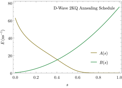
Figure 1: Native annealing schedule of the D-Wave 2000Q low noise processor.

We now consider the quantum annealing problem defined by a system Hamiltonian of the form

$$H_{S}(s)=\frac{A(s)}{2}H_{X}+\gamma\frac{B(s)}{2}H_{Z}\,,$$ (3)

where

$$H_{X}=-\sum_{i}\sigma_{i}^{x},\qquad H_{Z}=\sum_{i}h_{i}\sigma_{i}^{z}+\sum_{i<j}J_{ij}\sigma_{i}^{z}\sigma_{j}^{z}\ .$$ (4)

and $\gamma\in(0,1]$ is a scaling factor that controls the energy scale of the computational problem. We refer to $A(s)$ and $B(s)$ as the physical schedules of the anneal. They are fixed properties of the quantum annealing hardware (see Fig. 1), but $s$ can be made to depend on $\tau=t/t_{f}$, in the adjustable way that we describe below for the DW2KQ. We call the function $s(\tau)\mathrel{\mathop{\mathchar 58\relax}}[0,1]\mapsto[0,1]$ the control schedule.

We model the anneal according to the AME Albash et al. (2012) with the Hamiltonian in Eq. (3). The AME is derived from the total Hamiltonian $H(t)=H_{S}(t)+H_{B}+H_{SB}$, with $H_{SB}=g\sum_{i}A_{i}\otimes B_{i}$ where the $A_{i}$ ($B_{i}$) are the dimensionless system (bath) operators, subject to an adiabatic approximation. The resulting Liouvillian is of the time-dependent Davies form

$$\mathcal{L}(t) =-i\left[H_{S}(t)+H_{LS}(t),\bullet\right]+\mathcal{D}(t)$$ (5a)

$$\mathcal{D}(t) =\sum_{ij\omega}\gamma_{ij}(\omega)\Big{(}A_{j}(\omega)\bullet A_{i}^{\dagger}(\omega)$$

$$\qquad-\frac{1}{2}\left\{A_{i}^{\dagger}(\omega)A_{j}(\omega),\bullet\right\}\Big{)}\ .$$ (5b)

Here $H_{LS}(t)$ is the Lamb-shift term, $\gamma_{ij}(\omega)$ is the Fourier transform of the bath correlation function

$$G_{ij}(t_{1},t_{2})=\langle B_{i}(t_{1})B_{j}(t_{2})\rangle=G_{ij}(t_{1}-t_{2})\ ,$$ (6)

$B_{i}(t)=e^{iH_{B}t}B_{i}e^{-iH_{B}t}$, $\langle X\rangle=\mathrm{Tr}(\rho_{B}X)$ where $\rho_{B}$ is the initial bath state, and $\omega(t)$ are the Bohr frequencies of $H_{S}(t)$ (to simplify notation we suppress their explicit time-dependence when convenient), i.e., the differences between the instantaneous eigenenergies of $H_{S}(t)$. The Lindblad operators $A_{i}(\omega)$ that appear in the Davies generator (“dissipator”) $\mathcal{D}$ are defined by

$$e^{irH_{S}(t)}A_{i}e^{-irH_{S}(t)}=\sum_{\omega}e^{-ir\omega}A_{i}(\omega)\ ,$$ (7)

i.e.,

$$A_{i}(\omega)=\sum_{E_{b}-E_{a}=\omega}\Pi_{a}A_{i}\Pi_{b}\ ,$$ (8)

where $H_{S}=\sum_{a}E_{a}\Pi_{a}$ and $\Pi_{a}$ are the eigenprojectors of $H_{S}$.

The Lamb shift is given by

$$H_{LS}=\sum_{ij\omega}S_{ij}(\omega)A_{i}^{\dagger}(\omega)A_{j}(\omega)\ ,$$ (9)

with

$$S_{ij}(\omega)=\int_{-\infty}^{+\infty}d\omega^{\prime}\gamma_{ij}(\omega^{\prime})\mathcal{P}\left(\frac{1}{\omega-\omega^{\prime}}\right)\ ,$$ (10)

where $\mathcal{P}$ is the Cauchy principal value. It commutes with $H_{S}$.

This master equation generates a completely positive map and describes a system with a slowly varying system Hamiltonian $H_{S}(t)$, weakly interacting with an infinite bath. Moreover $\mathcal{L}(t)$ has the property that it has the Gibbs state as a steady state, i.e., $\mathcal{L}(t)\sigma(t)=0$ with $\sigma(t)=e^{-\beta H_{S}(t)}/Z(t)$, $Z(t)=\mathrm{Tr}e^{-\beta H_{S}(t)}$.

In our simulations we assume longitudinal field coupling, i.e., the system operators in the system-bath interaction Hamiltonian are $A_{i}=\sigma_{i}^{z}$ with $\gamma_{ij}(\omega)=\delta_{ij}\gamma(\omega)$ (independent coupling) and the bath has an Ohmic spectral density, so that

$$\gamma(\omega)=2\pi\eta_{0}g^{2}\frac{\omega}{1-e^{-\beta\omega}}\ .$$ (11)

II.3 A modified BCT

Unfortunately, we cannot directly apply Prop. 1 to annealers with $A(t_{f})=0$ (such as the DW2KQ) because of the following result (proven in App. A):

Proposition 3

Assume that $\mathcal{L}(\tau)$ is the AME Liouvillian [Eq. (5a)] with the Hamiltonian in Eq. (3) and longitudinal system-bath coupling (i.e., that commutes with $H_{Z}$). Then, at the end of the anneal when $A(t_{f})=0$, the zero eigenvalue of $\mathcal{L}(t_{f})$ is at least $d$-fold degenerate, where $d$ is the system’s Hilbert space dimension.

Since presumably, when $A(t)\neq 0$ for $t<t_{f}$ the Lindbladian $\mathcal{L}(t)$ has a unique steady state $\sigma(t)$ which corresponds to its zero eigenvalue, Prop. 3 means that the Liouvillian gap closes at $t_{f}$ and we cannot use Prop. 1.

We now generalize the BC result Prop. 1 to the situation where one enforces the BC conditions at the same point as where the Liouvillian gap closes, e.g., at $t=t_{f}$.

Proposition 4

Assume that $\left\|\mathcal{L}(\tau)\right\|_{1,1}$ is summable in $\tau\in[0,1]$, $\mathcal{L}(\tau)$ is differentiable to order $k+2$ in a neighborhood of $\tau=1$, and generates a trace-preserving and hermiticity-preserving contractive semigroup, i.e., $\left\|e^{r\mathcal{L}(\tau)}\right\|_{1,1}\leq 1$ for all $r\geq 0$, $\tau\in\left[0,1\right]$. Suppose $\mathcal{L}(\tau)$ has a unique steady state $\sigma(\tau)$ at each time $\tau\in[0,1]$ except at the point $\tau_{0}=1$ where the Liouvillian gap closes as $\Delta\simeq v(\tau_{0}-1)^{\alpha}$ for a linear schedule (i.e., in the absence of a BC schedule). Let $\rho(\tau)$ be the solution of Eq. (1) with initial condition $\rho(0)=\sigma(0)$ and $\sigma(1^{-})\mathrel{\mathop{\mathchar 58\relax}}=\lim_{r\to 1^{-}}\sigma(r)$. Assume we enforce boundary cancellation at the end, i.e., $\mathcal{L}(\tau)$ has vanishing derivatives at $\tau=1$ to order $k$: $\left.\partial_{\tau}^{(j)}\mathcal{L}\right|_{\tau=1}=0$ $\forall j=1,2,\ldots,k$ [note that here $\mathcal{L}(s(\tau))$ is written for simplicity as $\mathcal{L}(\tau)$]. Then boundary cancellation is only mildly effective in that the adiabatic error satisfies

$$\left\|\rho(1)-\sigma(1^{-})\right\|_{1} \leq\frac{C}{t_{f}^{\eta}}\ ,$$ (12a)

$$\mathrm{with\,\,} \eta=\frac{k+1}{k\alpha+\alpha+1}<\frac{1}{\alpha}.$$ (12b)

The proof is given in App. B, which also discusses the relaxed smoothness assumptions of Prop. 1 relative to Ref. Campos Venuti and Lidar (2018). The fact that the gap closes for the Lindbladian modeling the D-Wave annealers was already noted in Ref. Venuti et al. (2016), and indeed Eq. (12b) with $k=0$ was derived there.

For completeness we comment also on the case where the Liouvillian gap closes in the middle of the evolution and one enforces boundary cancellation at the end. We have performed numerical simulations under these conditions (see App. C), all agreeing with a scaling of the adiabatic error as in Eq. (12a), but with an exponent given by $\eta=k+1$, as in Eq. (2). Analytical results will be presented elsewhere.

Summarizing, if the gap closes at the end of the evolution, implementing BC is mildly advantageous in that the best one can do is to change the exponent $\eta$ from $1/(\alpha+1)$ to $1/\alpha$ for an infinitely flat schedule ($k\to\infty$). If, instead, the gap closes in the middle of the evolution, we infer from our numerical results that is has no effect on the scaling of the adiabatic error and implementing BC results in a favorable exponent $\eta=k+1$, just as in the case where the Liouvillian gap does not close at all.

II.4 Freezing

As the Hamiltonian starts to commute with the system-bath coupling operators near the end of the anneal, the dynamics of the system will begin to slow down. This gives another significant consideration regarding the successful implementation of BC schedules, which is that the system state appears to stop evolving at a point $t_{0}<t_{f}$, a phenonemon of quantum annealing called freezing. To explain freezing, we write the master equation in the instantaneous energy eigenbasis $\{|n\rangle\}$, $n=0,1,\ldots,d-1$ (we omit the time dependence for clarity), i.e., the basis which diagonalizes the Hamiltonian $H_{S}(t)$. Consider the region of the anneal where $A\left(t\right)$ is small but non-zero, and also $B(t)>0$. It is then natural to assume that the spectrum of $H_{S}(t)$ is non-degenerate. The density matrix in the energy basis is $\rho(t)=\sum_{mn}\rho_{mn}|m\rangle\!\langle n|$. The diagonal elements of $\rho$ in this basis evolve according to the Pauli master equation Pauli (1928) (for a modern derivation see, e.g., Ref. Lidar (2019b)). In particular, the ground state probability $\rho_{00}=\langle 0|\rho(t)|0\rangle$ evolves according to

$$\dot{\rho}_{00} =\sum_{n}\left(\rho_{nn}W_{0n}-\rho_{00}W_{n0}\right)$$ (13a)

$$=\sum_{n>0}W_{0n}\left(\rho_{nn}-\rho_{00}e^{-\beta\left(E_{n}-E_{0}\right)}\right)\ ,$$ (13b)

where the transition rate matrix $W$ has the following matrix elements:

$$W_{mn}=\sum_{i,j}\gamma_{ij}(E_{n}-E_{m})\langle m|\sigma_{j}^{z}|n\rangle\langle n|\sigma_{i}^{z}|m\rangle.$$ (14)

On the basis of Eqs. (13) and (14), freezing is seen to be a consequence of the following argument. Since we are in the adiabatic regime, only the lowest levels are populated, i.e., $\rho_{nn}\simeq 0$ for $n$ greater than some $n_{A}$. Eq. (13) is then replaced by

$$\dot{\rho}_{00} \simeq\sum_{n=1}^{n_{A}}W_{0n}\left(\rho_{nn}-\rho_{00}e^{-\beta\left(E_{n}-E_{0}\right)}\right)$$ (15a)

$$\qquad-\rho_{00}\sum_{n=n_{A}+1}^{d}W_{0n}e^{-\beta\left(E_{n}-E_{0}\right)}\ ,$$ (15b)

where $d$ is the system’s Hilbert space dimension. When $A(t)=0$, the Hamiltonian is diagonal in the computational basis. Let the Hamming distance between the ground state $|0\rangle$ and the excited states $\{|n\rangle\}_{n=1}^{n_{A}}$ when $A(t)=0$ be at least $q$ (note that $q\geq 1$). Using perturbation theory around $A(t)=0$ it can be shown that $\langle 0|\sigma_{j}^{z}|n\rangle=O\left(A^{q}\right)$; see App. D. Hence, at the time $t_{0}$ at which $A$ is sufficiently small (but non-zero) one has $W_{0n}=O(A^{2q})\simeq 0$ for $n=1,2,\ldots,n_{A}$, and we can neglect the sum in line (15a); we determine $t_{0}$ below. As for the term in line (15b), the transition rates between higher excited states are typically smaller, and moreover, the terms are exponentially suppressed because of the larger gaps (i.e., for sufficiently small temperatures $E_{n}-E_{0}\gg 1/\beta$, given that $n\geq n_{A}+1\geq 2$). As a consequence, Eq. (15) becomes $\dot{\rho}_{00}\approx 0$, i.e., the ground state population is effectively frozen for $t\geq t_{0}$.

The location of the freezing point for the $n$th excited state is determined by the point where the relaxation time for the $n$th excited state, given by $\tau_{\text{rel}}^{(n)}=W_{0n}^{-1}$, becomes longer than the anneal time. As long as just one of these relaxation times, with $n\in\{1,\ldots,n_{A}\}$ is too long, the system will not thermalize. For the system to freeze, i.e., $\dot{\rho}_{00}\approx 0$, we need all transitions to cease. Hence, we define the freezing point as the solution $t_{0}$ of $\min_{n\in\{1,\ldots,n_{A}\}}\tau_{\text{rel}}^{(n)}=t_{f}$, or:

$$t_{0}\mathrel{\mathop{\mathchar 58\relax}}=\{\min t\in[0,t_{f}]\text{ s.t. }\max_{n\in\{1,\ldots,n_{A}\}}W_{0n}(t)=1/t_{f}\}\ .$$ (16)

In terms of the control schedule $s(\tau)$, we have $s_{0}\mathrel{\mathop{\mathchar 58\relax}}=s(\tau_{0})$, where $\tau_{0}=t_{0}/t_{f}$. In practice, to determine the freezing point $s_{0}$ we implement a closely related procedure described in App. E.

Note that, as a consequence of the perturbative argument, (for sufficiently small $A$) the rates $W_{0n}$ are decreasing functions of $A$. So if $A(t)$ is decreasing in $t$, $W_{0n}$ can be considered zero for $t\geq t^{\ast}$. A similar argument works when substituting $0\leftrightarrow m$, and one finds that the population in the $m$th excited state, $\rho_{mm}$, is frozen, albeit with possibly different freezing points than given by Eq. (16).

Another consequence of this argument is that the phenomenon of freezing should be more pronounced (i.e., occur for smaller $t_{0}$ and resulting in smaller $\dot{\rho}_{00}$ for $t>t_{0}$) for those problems where the ground state is separated by a large Hamming distance from the excited states, i.e., a larger tunneling barrier such as the T-gadget compared to the FM-gadget, discussed in Sec. III.2 below. These problems are the ones which are harder to simulate with standard classical simulated annealing with single spin flip moves Kirkpatrick et al. (1983) (cluster flip moves Zhu et al. (2015) would not necessarily be similarly affected).

Finally, note that a simulation of a master equation to which the considerations above apply, such as the AME (see Sec. II.2), is also expected to exhibit freezing.

II.5 Boundary cancellation with a ramp at the end

Since the ground state population does not change past the freezing point, no change in the schedule would be effective if performed after freezing. In view of these considerations we perform BC before freezing sets in, which — for the standard control schedule $s(\tau)=\tau$ (see Fig. 1) — happens for $s\approx 0.55$, depending on the problem. Our strategy will be the following. First, evolve from $t=0$ to $t_{f}$ with a BC schedule. To avoid freezing, we ensure that $A(t_{f})\neq 0$ at the end of the BC schedule. Thus, $t_{f}$ does not correspond to the usual total anneal time for which $A(t_{f})=0$. Right after the BC schedule ends, we perform a linear ramp of duration $t_{r}=1\,\mu$s until the schedules reach their final values (in particular $A(t_{f}+t_{r})=0$), after which the system is measured in the computational basis. The state after the entire evolution can be written as $\mathcal{E}_{\mathrm{ramp}}\mathcal{E}_{\mathrm{BC}}\rho(0)$, where $\mathcal{E}_{\mathrm{BC}}$ ($\mathcal{E}_{\mathrm{ramp}}$) is the evolution through the BC schedule (ramp). However, random local fields and coupler perturbations [integrated control errors (ICE)] result in a Hamiltonian that does not behave as intended in the ideal case Albash et al. (2019), and these errors have been well documented in the D-Wave processors dwa . The effect of such random perturbations can be controlled with error suppression and correction Young et al. (2013); Pudenz et al. (2014); Pearson et al. (2019a), which will be employed below for the ferromagnetic chain gadget. Due to this ICE effect, the measured state is better represented by

$$\rho_{\mathrm{final}}\mathrel{\mathop{\mathchar 58\relax}}=\mathsf{E}_{J}\left[\mathcal{E}_{\mathrm{ramp}}\mathcal{E}_{\text{BC}}\rho(0)\right]\ ,$$ (17)

where we denoted by $\mathsf{E}_{J}\left[\bullet\right]$ the average over the noise on the random couplings $J_{ij}$ and fields $h_{i}$.

Let us now define $\rho(t_{f})\mathrel{\mathop{\mathchar 58\relax}}=\mathcal{E}_{\text{BC}}\rho(0)$, while $\sigma(t_{f})$ is the Gibbs state at the end of the BC schedule [recall that $\rho(0)=\sigma(0)$], corresponding to the Hamiltonian in Eq. (3). The adiabatic theorem in its various forms, including with boundary cancellation, provides an upper bound on the pre-ramp distance $\|\delta\|_{1}$, where $\delta\mathrel{\mathop{\mathchar 58\relax}}=\rho(t_{f})-\sigma(t_{f})$. Defining

$$\sigma_{\mathrm{final}}\mathrel{\mathop{\mathchar 58\relax}}=\mathsf{E}_{J}\left[\mathcal{E}_{\mathrm{ramp}}\sigma(t_{f})\right]\ ,$$ (18)

$\delta$ can be related to $\rho_{\mathrm{final}}$ and $\sigma_{\mathrm{final}}$ via the following bound:

$$\left\|\rho_{\mathrm{final}}-\sigma_{\mathrm{final}}\right\|_{1} =\left\|\mathsf{E}_{J}[\mathcal{E}_{\mathrm{ramp}}\delta]\right\|_{1}$$ (19a)

$$\leq\mathsf{E}_{J}\left[\left\|\mathcal{E}_{\mathrm{ramp}}\delta\right\|_{1}\right]$$ (19b)

$$\leq\mathsf{E}_{J}\left[\left\|\delta\right\|_{1}\right]\ .$$ (19c)

Here Eq. (19b) follows from from Jensen’s inequality Jensen (1906) and the fact that every norm is convex (implying $\left\|\mathsf{E}_{J}\left[x\right]\right\|_{1}\leq\mathsf{E}_{J}\left[\left\|x\right\|_{1}\right]$), while Eq. (19c) follows because $\mathcal{E_{\mathrm{ramp}}}$ is a completely positive and trace-preserving (CPTP) map Nielsen and Chuang (2010) (implying $\left\|\mathcal{E}_{\mathrm{ramp}}\delta\right\|_{1}\leq\left\|\delta\right\|_{1}$). Note that $\rho_{\mathrm{final}}$ is the empirically measured state, while $\sigma_{\mathrm{final}}$ differs from the state that we sought to prepare $\sigma(t_{f})$, by the presence of the extra operations $\mathsf{E}_{J}\left[\mathcal{E}_{\mathrm{ramp}}\bullet\right]$.

The bound (19) implies a similar bound for the ground state probabilities. Let us define

$$P_{\text{GS}} \mathrel{\mathop{\mathchar 58\relax}}=\mathrm{Tr}\left[|\text{GS}\rangle\!\langle\text{GS}|\rho_{\mathrm{final}}\right]$$ (20a)

$$P_{\text{GS}}^{*} \mathrel{\mathop{\mathchar 58\relax}}=\mathrm{Tr}\left[|\text{GS}\rangle\!\langle\text{GS}|\sigma_{\mathrm{final}}\right]\ ,$$ (20b)

where $|\text{GS}\rangle$ is the ground state of the Hamiltonian at the end of the anneal, i.e., the ground state of $H_{Z}$. Since

$$\left|\mathrm{Tr}\left[|\text{GS}\rangle\!\langle\text{GS}|x\right]\right|\leq\left\||\text{GS}\rangle\!\langle\text{GS}|\right\|_{\infty}\left\|x\right\|_{1}=\left\|x\right\|_{1}\ ,$$ (21)

it follows that the adiabatic error defined as

$$D_{\text{GS}}\mathrel{\mathop{\mathchar 58\relax}}=\left|P_{\text{GS}}-P_{\text{GS}}^{*}\right|\ ,$$ (22)

satisfies

$$D_{\text{GS}}\leq\left\|\rho_{\mathrm{final}}-\sigma_{\mathrm{final}}\right\|_{1}\ .$$ (23)

The adiabatic error quantifies the difference between the ground state overlaps of the experimentally measured state ($\rho_{\mathrm{final}}$) and the Gibbs state ($\sigma_{\mathrm{final}}$).

II.6 An adiabatic error bound that combines everything

Combining Eqs. (19) and (23) with Props. 1 and 4 and our numerical evidence, we obtain

$$D_{\text{GS}}\leq\left\|\rho_{\mathrm{final}}-\sigma_{\mathrm{final}}\right\|_{1} \leq\frac{C}{t_{f}^{\eta}}\ ,$$ (24)

where $C$ is now the noise averaged constant ($\mathsf{E}_{J}\left[\bullet\right]$) and $\eta$ depends on the physical assumptions. Namely, $\eta=k+1$ if the Liouvillian either has a non-zero spectral gap throughout the anneal or if BC is enforced after the Liouvillian gap has already closed somewhere along the anneal, while $\eta=(k+1)/(k\alpha+\alpha+1)$ if the Liouvillian gap closes at the same point at which BC is enforced (Prop. 4).

Of course we may reformulate Eq. (24) as a bound on $P_{\text{GS}}$:

$$P_{\text{GS}}^{*}-\frac{C}{t_{f}^{\eta}}\leq P_{\text{GS}}\leq P_{\text{GS}}^{*}+\frac{C}{t_{f}^{\eta}}\ .$$ (25)

II.7 Anomalous heating

Our discussion so far has assumed that the effective temperature of the system remains constant as a function of both the anneal parameter $\tau=t/t_{f}$ and the total anneal time $t_{f}$. However, there is evidence to suggest that the latter is in fact not the case in the D-Wave devices, i.e., the temperature is $t_{f}$-dependent. The reason is an unintentional but omnipresent high-energy photon flux that enters the D-Wave chip from higher temperature stages through cryogenic filtering, which accumulates over long anneal times and manifests as an effectively higher on-chip temperature ano . This anomalous heating phenomenon will hinder our ability to test the BCP, since it means that in fact $P_{\text{GS}}^{*}$ is a function of $t_{f}$, which complicates testing the BCT prediction as summarized by Eq. (25). Indeed, for a Gibbs state $\sigma_{\text{final}}=e^{-\beta H_{S}}/Z$ (with $\beta$, $H_{S}$, and the partition function $Z$ all evaluated at $t=t_{f}$), expanding $H_{S}$ in its eigenbasis as $H_{S}=\sum_{i=0}E_{i}|{i}\rangle\!\langle i|$ we readily find

$$P_{\text{GS}}^{*}=\langle\text{GS}|\sigma_{\mathrm{final}}|\text{GS}\rangle=\frac{1}{1+\sum_{i=1}e^{-\beta(t_{f})\Delta_{i}}}\ ,$$ (26)

where $\ket{0}$ is the ground state and $\Delta_{i}\mathrel{\mathop{\mathchar 58\relax}}=E_{i}-E_{0}$.

Assuming for simplicity that $\beta(t_{f})=\beta_{0}+a/t_{f}$, i.e., a temperature that depends linearly on $t_{f}$ with rate $a>0$, and that $1\ll\beta(t_{f})\Delta_{1}\ll\beta(t_{f})\Delta_{i}$ for $i\geq 2$, we can write this as

$$P_{\text{GS}}^{*}\approx 1-e^{-\beta(0)\Delta_{1}}e^{-a\Delta_{1}/t_{f}}\ ,$$ (27)

i.e., the algebraic scaling with $t_{f}$ of Eq. (25) becomes obscured by an exponential scaling due to $P_{\text{GS}}^{*}$.

However, in reality we do not know the functional form of $\beta(t_{f})$, and the assumption $1\ll\beta(t_{f})\Delta_{1}\ll\beta(t_{f})\Delta_{i}$ may not hold. Therefore, in the analysis of our experimental results in Sec. IV below, we instead use an ansatz of the form

$$P_{\text{GS}}=\bar{P}_{\text{GS}}^{*}+\frac{C^{\prime}}{t_{f}^{\eta^{\prime}}}\ ,$$ (28)

where $\bar{P}_{\text{GS}}^{*}$ is a free fitting parameter representing an averaged value of the true (unknown) $P_{\text{GS}}^{*}(t_{f})$, $C^{\prime}$ becomes another fitting parameter which already accounts for noise averaging as explained in Sec. II.6, and $\eta^{\prime}$ plays the role of the effective scaling exponent, i.e., our proxy for $\eta$ in Eq. (25).

III Methods

III.1 Boundary Cancellation Protocol (BCP)

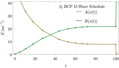
Figure 2: An example of the D-Wave boundary cancellation protocol with the $\beta_{2}$ schedule ramped at $s_{\text{BC}}=0.50$, with the constructed parametric schedule (top) and the corresponding physical schedules (bottom). For the schedule shown here we chose an anneal time of $t_{f}=100\,\mu$s. The ramp duration is $t_{r}=1\mu$s. Contrast with the native schedule of the DW-LN processor shown in Fig. 1. The most significant impact is on the $B(s)$ schedule, which is not natively flat, in contrast to the $A(s)$ schedule, which natively approaches $0$ in a very flat manner.

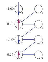
(a)  

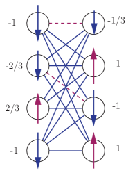
(b)  

Figure 3: Illustration of the FM-gadget (a) and T-gadget (b) embedded into the Chimera architecture as represented by an Ising Hamiltonian $H_{Z}$ [Eq. (4)]. Ferromagnetic (blue) and anti-ferromagnetic (dashed purple) couplings all have the same strength of $J_{ij}=-1$ and $J_{ij}=1$, respectively. Local fields $h_{i}$ are indicated by the arrows and their value beside them. The ordering of the qubits in the Chimera architecture is also enumerated in (a).

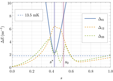
(a)  FM-gadget

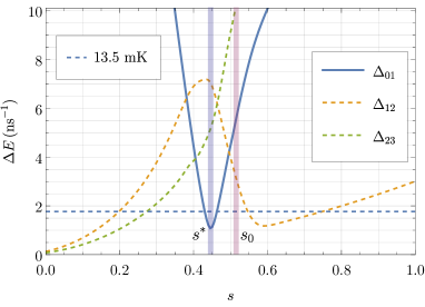
(b)  T-gadget

Figure 4: Spectral gaps of (a) the FM-gadget and (b) the T-gadget (with $\gamma=0.5$), as the schedule is varied according to typical physical schedules $A(s)$ and $B(s)$ of the D-Wave processor (App. F), shown in units of $\mathrm{ns}^{-1}$ ($\hbar=1$). The notation $\Delta_{n,n+1}$ denotes the energy gap between the $n$th and $n+1$th Hamiltonian eigenstates, with $n=0$ being the ground state. The $13.5\,\mathrm{mK}$ energy scale is also shown, which is the reported dilution fridge temperature of the DW-LN processor. The minimum gap location is $s^{*}=0.43$ for the FM-gadget and $s^{*}=0.44$ for the T-gadget. The minimum gap region is marked by the light blue shading, while the estimated start of frozen dynamics at $s_{0}$ is marked by pink shading, found by solving Eq. (16) (see App. E for details). Note that for both gadgets, the first, second, and third excited states are all initially degenerate in the subspace of a single $\ket{-}$ excitation of the transverse-field ground state. The nonzero excited state gaps $\Delta_{12}$ and $\Delta_{23}$ of the FM gadget ($\Delta_{12}$ only for the T gadget) at $s=1$ are the result of symmetry breaking due to a crosstalk term we included in the Hamiltonian, of strength $\chi=0.02$ (see App. G). The avoided level crossing of the T-gadget is slightly narrower than that of the FM-gadget.

We performed most of our experiments with the D-Wave 2000Q low noise (DW-LN) processor accessed through D-Wave Leap. We also performed additional experiments with the D-Wave 2000Q processor at the NASA Quantum Artificial Intelligence Laboratory (DW-NA) as well as the D-Wave Advantage (DWA) processor through D-Wave Leap. In the processor specifications, the hardware-determined schedules $A(s)$ and $B(s)$ are parametrized by the user-defined control schedule $s(\tau)$. In the standard case the control is linear, i.e., $s(\tau)=\tau$ but in general $s(\tau)$ can be programmed in a piecewise linear manner as a function of time. The processor permits a maximum of $12$ points to specify the piecewise linear function $s(\tau)$. We take advantage of this enhanced capacity to approximate a BC schedule. The allowed range of programmable anneal times is $t_{f}\in[1,2000]\,\mu$s.

Even though $A(s)$ and $B(s)$ themselves need not satisfy the vanishing derivative requirement of the BCP, it follows from the chain rule that $A(s(t))$ and $B(s(t))$ do, as long as the control schedule $s(t)$ satisfies this requirement and $A(s)$ and $B(s)$ are differentiable to the same order as $s(t)$. To be concrete, we take

$$s(\tau)=\beta_{k}(\tau)\ ,\qquad\tau=t/t_{f}\ ,$$ (29)

where

$$\beta_{k}(\tau) \mathrel{\mathop{\mathchar 58\relax}}=\frac{\mathrm{B}_{\tau}(1,k+1)}{\mathrm{B}_{1}(1,k+1)}$$ (30a)

$$=1-(1-\tau)^{k+1}$$ (30b)

is the regularized incomplete beta function of order $k$ Rezakhani et al. (2010); Campos Venuti and Lidar (2018), with

$$\mathrm{B}_{x}(a,b)\mathrel{\mathop{\mathchar 58\relax}}=\int_{0}^{x}y^{a-1}(1-y)^{b-1}dy$$ (31)

being the incomplete beta function. As is apparent from Eq. (30b), the function $\beta_{k}(\tau)$ has exactly $k$ vanishing $\tau$-derivatives at $\tau=1$, as required by the BCT. We refer to this class of control schedules simply as beta schedules.

As we discussed above, in contrast to the theoretical setup of Ref. Campos Venuti and Lidar (2018), due to freezing there is no practical advantage to flattening the schedule as $s$ approaches $1$. The effectiveness of the BCP is most apparent when the flattening of the schedule occurs after the avoided level crossing of the anneal (at $s=s^{*}$), but before the dynamics freeze (at $s=s_{0}$). Thus, rather than using the standard schedules $\{A(s),B(s)\}$ with linear $s(\tau)$ that freeze out around $s\simeq 0.5$, the beta schedule needs to be adjusted so that it terminates at an appropriate point $s_{\text{BC}}$ corresponding to $t=t_{f}$ and satisfying $0<s^{*}<s_{\text{BC}}<s_{0}\leq 1$, rather than always at $s=1$, when the open system dynamics are already frozen out. The anneal is then ramped to the final values $A(t_{f}+t_{r})=0$ and $B(t_{f}+t_{r})$. The precise construction of the control schedule is given in App. F.

Note that the piecewise linear approximation of Eq. (29) cannot exactly satisfy the requirement of vanishing derivatives at the end. However, Ref. (Campos Venuti and Lidar, 2018, Prop. 3) shows that (at least for the case $k=1$) if one tries to enforce a vanishing derivative but achieves only approximate vanishing, the overall adiabatic error is diminished nonetheless. A reasonable expectation is that the scaling will be milder than the theoretical ideal of $1/t_{f}^{k+1}$ for Liouvillians with a spectral gap (Prop. 1), i.e., will be of the form $1/t_{f}^{\eta}$ with $\eta<k+1$ for schedules that only approximate the desired $\beta_{k}$ schedule. An example of this schedule construction is shown in Fig. 2.

III.2 8 Qubit Gadgets

We briefly describe the two gadgets utilized in our experiments, which are both illustrated in Fig. 3 along with their couplings and bias values in the Hamiltonian $H_{Z}$ in Eq. (4). The first gadget we use is an 8-qubit ferromagnetic (FM) chain, depicted in Fig. 3 using its embedding in a single unit cell of the Chimera graph in the D-Wave 2000Q processor, which is a bipartite $K_{4,4}$ graph. The local fields in this gadget were adjusted to break the most significant degeneracies in the ground subspace and first excited subspace that are present in a simple ferromagnetic chain without any fields. This gadget thus enforces a large Hamming distance between its ground state and any first exited state without introducing additional two-body interactions. The remaining degeneracy in the first excited state is broken by crosstalk interactions in the device, which we model and include in simulations of the Hamiltonian (see App. G). In addition, it is simple to tile and embed the QAC encoding of the FM-gadget (see below) on the Chimera graph.

The second gadget we utilize is the one introduced in Ref. Albash and Lidar (2018). This gadget was thoroughly analyzed there and established to pose a small-gap tunneling barrier between the ground state and the first excited state, so we refer to it as the “T-gadget”. For finer control of the energy gap, the T-gadget is scaled to $\gamma=0.5$ [recall Eq. (3)]. The ground state of both gadgets is the all-$0$ state, denoted by $|\mathbf{0}\rangle$. Both gadgets also share the all-$1$ state $|\mathbf{1}\rangle$ as their first excited state.

The spectral gaps of the gadgets are shown in Fig. 4. The most crucial distinction between them is that the FM-gadget has a minimum gap $\Delta_{01}(s^{*})$ to the first excited state that is larger than the dilution fridge operating temperature, while the opposite holds for the T-gadget. Figure 4 suggests that implementing the BCP with the termination point $s_{\text{BC}}$ somewhere in the range of $[0.45,0.50]$ will be the most effective for both gadgets, since $s^{*}\approx 0.43$ and $s_{0}\approx 0.5$. Before this range, the BCP spends more time slowing down before the minimum gap, while after this range it goes through the minimum gap too quickly and only slows down going into the freezing phase.

III.3 Encoding with Quantum Annealing Correction

We supplement the BCP with quantum annealing correction (QAC) Pudenz et al. (2014) and compare the scaling improvement versus QAC with a simple linear anneal. The QAC encoding of the computational Hamiltonian in (3) has the form

$$H_{\text{QAC}}=\overline{H}_{Z}+\lambda H_{P}$$ (32)

where $\overline{H}_{Z}$ is an $m$-qubit repetition of the problem Hamiltonian $H_{Z}$ wherein each $\sigma_{i}^{z}$ and $\sigma_{i}^{z}\sigma_{j}^{z}$ term is replaced by its encoded counterpart $\overline{\sigma_{i}^{z}}=\sum_{\ell=1}^{m}\sigma_{i_{\ell}}^{z}$ and $\overline{\sigma_{i}^{z}\sigma_{j}^{z}}=\sum_{\ell=1}^{m}\sigma_{i_{\ell}}^{z}\sigma_{j_{\ell}}^{z}$, respectively, and the penalty Hamiltonian imposes an energy cost by ferromagnetic coupling to an ancilla penalty-qubit,

$$H_{P}=-\sum_{i}(\sigma_{i_{1}}^{z}+\ldots+\sigma_{i_{m}}^{z})\sigma_{i_{p}}^{z}.$$ (33)

Here the index $i$ is over the logical qubits, $i_{1}\ldots i_{m}$ are the physical qubits corresponding to the logical qubit $i$, and $i_{p}$ is the ancilla for qubit $i$. A majority vote over the results of the measurement on the computational basis of the (odd) $m$ physical qubits decides the spin value of logical qubit $i$. This strategy of combining an energy penalty against errors anticommuting with $H_{P}$ (the sum of the stabilizer generators of the bit-flip code) Jordan et al. (2006); Marvian and Lidar (2014); Bookatz et al. (2015); Jiang and Rieffel (2017); Marvian and Lidar (2017a, b); Lidar (2019a), along with a bit-flip repetition code, has been demonstrated numerous times to be successful at enhancing the performance of quantum annealing, despite not being able to protect against pure dephasing errors (which commute with $H_{P}$) Pudenz et al. (2015); Mishra et al. (2015); Matsuura et al. (2016); Vinci et al. (2015); Matsuura et al. (2017); Pearson et al. (2019b). We only consider $m=3$ QAC encoding, which is naturally embedded onto the Chimera graph of all the DW2KQ processors. As the encoded FM-gadget can be naturally embedded with no additional minor embedding, we restrict our attention to it, and do not consider the T-gadget under QAC, which would require minor embedding. For the same reason we do not consider the more powerful nested QAC strategy Vinci et al. (2016); Vinci and Lidar (2018); Matsuura et al. (2019); Li et al. (2020), which is left for future work. We estimate the optimal penalty strength $\lambda$ for QAC by finding the value that maximizes the ground state probability of a simple linear anneal.

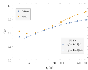
(a)  FM-gadget – $P_{\text{GS}}$

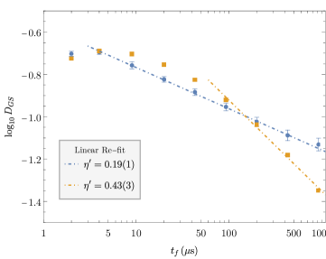
(b)  FM-gadget – $D_{\text{GS}}$

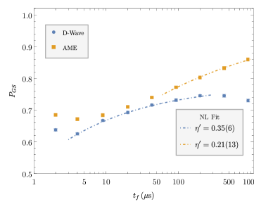
(c)  T-gadget – $P_{\text{GS}}$

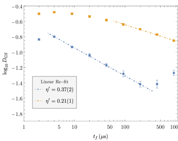
(d)  T-gadget – $D_{\text{GS}}$

Figure 5: DW-LN and AME results for $P_{\text{GS}}$ with a simple linear control schedule (without a ramp) for the FM-gadget [(a) and (b)] and the T-gadget [(c) and (d)]. A non-linear fit to (28) is applied on the data and yields estimates for $\eta^{\prime}$ as described in App. H. The initial constrained nonlinear fit to (28) yields values for $\eta^{\prime}$ and $\bar{P}_{\text{GS}}^{*}$ that may have high variance. A linear refit on $D_{\text{GS}}$ is done assuming $P_{\text{GS}}^{*}=\bar{P}_{\text{GS}}^{*}$ to refine $\eta^{\prime}$ with a smaller error. The values of $\eta^{\prime}$ and their associated uncertainties we find in this manner are reported in the legends. Error bars on the measured ground state probabilities represent $95\%$ confidence intervals. AME simulation parameters for both gadgets: $\eta_{0}g^{2}=5.0\times 10^{-4}$, $T=13.5$mK (see Sec. II.2) and crosstalk strength $\chi=0.02$ (see App. G).

IV Results

In this section we report on our results for $P_{\text{GS}}$, arising from both runs on the DW-LN and numerical simulations. As explained in Sec. II.7, we use Eq. (28) to fit our empirical results. Our data collection procedure is described in App. H.

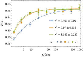
(a)  $s_{\text{BC}}=0.45$

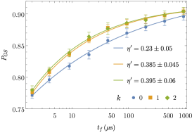
(b)  $s_{\text{BC}}=0.47$

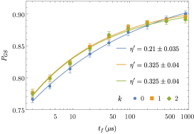
(c)  $s_{\text{BC}}=0.50$

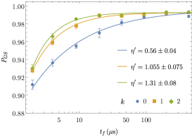
(d)  $s_{\text{BC}}=0.45$

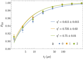
(e)  $s_{\text{BC}}=0.50$

Figure 6: DW-LN adiabatic distance scaling fits for the FM-gadget with BCP at (a) $s_{\text{BC}}=0.45$, (b) $s_{\text{BC}}=0.47$, and (c) $s_{\text{BC}}=0.50$ past the minimum gap location of $s^{*}\approx 0.43$ but before freeze-out at $s_{0}\approx 0.51$. (d) and (e): Adiabatic distance scaling of QAC encoded FM-gadget with BCP at $s_{\text{BC}}=0.45$ and $s_{\text{BC}}=0.50$ (see Sec. IV.4). Symbols represent the experimentally measured data points, solid lines are fits to $1/t_{f}^{\eta^{\prime}}$. The $\eta^{\prime}$ values reported in the legends an well as other parameters are obtained from nonlinear fits to the measured data as explained in App. H. Error bars represent $95\%$ confidence intervals.

IV.1 Linear control schedule ($k=0$)

We first consider the FM and T-gadgets under the native $A(s)$ and $B(s)$ schedules with linear control $s(\tau)=\tau$ and no ramp ($s_{\text{BC}}=1$), i.e., a standard quantum annealing protocol. This means that the anneal is stopped deep inside the frozen regime, i.e., freezing is expected to have a noticeable effect.

In Fig. 5 we plot, for both the FM-gadget and the T-gadget, the measured ground state probability $P_{\text{GS}}$ for the DW-LN, along with the same quantity obtained through AME simulations. We found $P_{\text{GS}}^{*}$ for DW-LN by a non-linear fit to the function $C^{\prime}/t_{f}^{\eta^{\prime}}+\bar{P}_{\text{GS}}^{*}$, where $C^{\prime}$ and $\eta^{\prime}$ are free parameters (left column of Fig. 5). In the AME case only the last four data points were used in the fit (since otherwise $t_{f}$ is too small, as evidenced by the curvature observed for small $t_{f}$ in the right column), while in the DW-LN case we dropped the first data point for both gadgets for the same reason. In the T-gadget case we also dropped the last two data points, as they are likely corrupted by anomalous heating (see Sec. II.7). This leads to the values $P_{\text{GS}}^{*}=0.97$ and $P_{\text{GS}}^{*}=0.78$ for the FM-gadget [Fig. 5(a)] and T-gadget [Fig. 5(c)], respectively. For the AME, we took $P_{\text{GS}}^{*}$ to be $1$, as this is consistent with the BCT for a large gap and the nonlinear fits did not find a smaller value. We then refined the value of $\eta^{\prime}$ by a linear fit to $\log_{10}(P_{\text{GS}}-P_{\text{GS}}^{*})$ as a function of $\log_{10}t_{f}$, since we expect $P_{\text{GS}}-P_{\text{GS}}^{*}$ to scale as $C/t_{f}^{\eta}$ by Eq. (25). Using Eqs. (24) and (25), we interpret $\log_{10}(P_{\text{GS}}-P_{\text{GS}}^{*})$ as a proxy for $\log_{10}D_{\text{GS}}$, plotted in Fig. 5(b) and Fig. 5(d) for the FM-gadget and T-gadget respectively.

Several observations are in order from Fig. 5.

• The $P_{\text{GS}}$ values at the largest $t_{f}$ are larger for the FM-gadget than for the T-gadget, in both the AME and DW-LN cases. This is consistent with the larger FM-gadget gap (see Fig. 4) and the larger tunneling barrier of the T-gadget (quantified by the ground state being separated by a larger Hamming distance from the excited states), which causes an earlier onset of freezing and hence “locks in” the smaller ground state population of the T-gadget.

• The FM gadget AME simulation has a larger $\eta^{\prime}$ ($0.43$) than the T-gadget ($0.21$). This signifies a faster convergence to the adiabatic limit of $P_{\text{GS}}=1$. This too is consistent with the larger FM-gadget gap and the larger tunneling barrier of the T-gadget. However, the opposite holds for the DW-LN $\eta^{\prime}$ values ($0.19$ vs $0.37$, for the FM and T-gadgets, respectively).

• The AME data for the T-gadget is in closer agreement with the power-law bound of the adiabatic theorem than the FM-gadget. This is evidenced by the good agreement with the linear fit in Fig. 5(d), but the persistence of some curvature at large $t_{f}$ in Fig. 5(b). We may speculate that the FM-gadget will transition to a power-law behavior at even larger $t_{f}$ than we were able to simulate, though one should keep in mind that in any case, the power-law bound of the adiabatic theorem is not tight.

• For the DW-LN at large $t_{f}$, we observe an appreciable reduction in $P_{\text{GS}}$ [Fig. 5(c)], and a concomitant increase in $D_{\text{GS}}$ [Fig. 5(d)] in the T-gadget case, and a small positive curvature in the FM-gadget case. This suggests that an anomalous excitation (heating) mechanism is at work in the D-Wave case for $t_{f}\gtrsim 300\mu$s. The source of this anomaly was discussed in Sec. II.7. The anomalous heating phenomenon hinders our ability to test the BCP, since it means that the effective temperature is itself $t_{f}$-dependent and increasing. As explained above, this is why we treated $P_{\text{GS}}^{*}$ as a fitting parameter.

• The DW-LN FM-gadget scaling [Fig. 5(b)] is much closer to the expected $D_{\text{GS}}\sim 1/t_{f}^{\eta}$ than the T-gadget [Fig. 5(d)], which is obscured by anomalous heating. It is unclear why this phenomenon should more severely impact the T-gadget.

We report the values of $\eta^{\prime}$ extracted from our fits in Fig. 5. To understand what value of $\eta^{\prime}$ to expect, note that according to our model of the D-Wave annealer and in view of Proposition 3, the Liouvillian gap $\Delta(\tau)$ must close at the end of the anneal. Recall that $\Delta\simeq v(\tau-\tau_{0})^{\alpha}$ with $\tau_{0}=1$ (or $t=t_{f}$) being the end of the anneal. We do not know the associated value of the exponent $\alpha$; however, given that $\mathcal{L}$ is a normal operator, if the Liouvillian depends smoothly on the schedule in a small interval around $t_{f}$, a standard result Kato (1995) implies that $\alpha$ must be an integer. On the other hand, $\alpha=1$ is incompatible with the fact that the lowest eigenvalue of $\mathcal{L}$ is zero, and that the gap must close smoothly. The value observed in the single qubit case is $\alpha=2$ Venuti et al. (2016). According to Prop. 4 and more specifically Eq. (12b) with $k=0$ (due to the linear schedule), this would correspond to an exponent $\eta=1/3$, which is also the scaling observed in the single qubit case Venuti et al. (2016).

However, as seen in Fig. 5(d), the AME T-gadget case has $\eta^{\prime}=0.21(1)$, which – when equated with $1/(\alpha+1)$ according to Eq. (12b) with $k=0$ – yields $\alpha=4$. This larger value of $\alpha$ (and corresponding smaller value of $\eta^{\prime}$) than was found in the single qubit case is not unexpected given the very different spectrum associated with the T-gadget.

As remarked above, in contrast to the T-gadget, the AME value of $\eta^{\prime}$ for the FM-gadget is at least $0.43$, and is likely to be slightly higher since the largest $t_{f}$ value for which we were able to run AME simulations appears to be too small for convergence. From Eq. (24) we expect $D_{\text{GS}}$ to scale with an exponent $\eta^{\prime}\geq\eta$, where for $k=0$ we have $1/(\alpha+1)\leq\eta\leq 1/\alpha$ [Eq. (12b)]. Thus $\eta^{\prime}\approx 0.43$ is consistent with these expectations for any integer $\alpha\geq 2$.

The DW-LN scaling is consistent with the expectation $\eta^{\prime}\geq\eta$ for the T-gadget, for which $\eta^{\prime}=0.37$. However, anomalous heating makes it difficult to be confident in the extracted $\eta^{\prime}$ value for this gadget. For the FM-gadget we find a good fit to $D_{\text{GS}}\sim 1/t_{f}^{\eta^{\prime}}$ with $\eta^{\prime}=0.19$, which could be explained by $\alpha=4$, as in the AME T-gadget case. However, the small positive curvature in the DW-LN FM-gadget data at large $t_{f}$ suggests that the true scaling may be obscured by anomalous heating here as well.

Since anomalous heating plays such a significant role in the T-gadget behavior at large $t_{f}$, we abandoned it for our experiments involving BCP schedules with $k\geq 1$. We focus for the rest of this work on the FM-gadget.

IV.2 BCP schedules with $k\geq 1$

We now turn to actual boundary cancellation schedules. In light of our discussion in Sec. II, a successful BCP must occur before the closing of the Liouvillian gap and freeze-out, while at the same time the Hamiltonian gap remains large enough to promote relaxation to the ground state. We thus apply the BCP at a point $s^{*}<s_{\text{BC}}<s_{0}$, such that $A(s_{\text{BC}})\neq 0$. The BC schedule is followed by a ramp of $1\,\mu\mathrm{s}$ to the final values of $A$ and $B$.

Following the same nonlinear fit procedure as in Sec. IV.1, we plot the DW-LN $P_{\text{GS}}$ results for the FM-gadget in Fig. 6. More specifically, Fig. 6(a)-6(c) shows the results for $s_{\text{BC}}\in\{0.45,0.47,0.50\}$, while Fig. 6(d)-6(e) shows analogous plots after applying QAC, which we discuss in Sec. IV.4.

The first observation that emerges from Fig. 6 is that the $\beta_{0}$ schedule results in a significantly larger (i.e., better) scaling exponent than the $k=0$ schedule of Sec. IV.1, for which we found $\eta^{\prime}=0.19$. The difference between the two is that for the case shown in Fig. 6 the schedule includes a ramp at $s=s_{\text{BC}}$. As the ramp point grows from $0.45$ to $0.47$ to $0.50$, the value of $\eta^{\prime}$ correspondingly declines from $0.47$ to $0.23$ to $0.21$. This confirms that stopping the BC schedule before freeze-out (at $s_{0}\approx 0.52$) has a significant positive impact on the performance of the BCP.

If the Liouvillian is gapped at the endpoint of the BC schedule, the theoretical expectation for the scaling of the adiabatic error is $\eta=k+1$ for the $\beta_{k}$ schedule (recall Sec. II.6). Instead, Figure 6 shows that the measured exponents $\eta^{\prime}$ exhibit a strong dependence on the value of $s_{\text{BC}}$. The most favorable case is $s_{\text{BC}}=0.45$ [Fig. 6(a)], for which the exponents $\eta^{\prime}$ are $\{0.47\ (k=0),\ 0.97\ (k=1),\ 1.1\ (k=2)\}$, i.e., roughly half that value for $k=0,1$. The $k=2$ exponent is statistically indistinguishable from that for $k=1$. It is likely that this is due to the fact that the relatively small number of schedule interpolation points does not allow us to approximate the ideal $\beta_{2}$ schedule sufficiently well (see Sec. IV.3 below). Other sources of error, such as ICE and anomalous heating, may also play a role.

While this level of agreement with the BCT for the gapped Liouvillian case is far from impressive, the dependence of $\eta^{\prime}$ on $k$ is less consistent with the BCT prediction for when the Liouvillian gap closes at $s_{\text{BC}}$; in this case Prop. 4 for $\alpha=1$ yields $\eta=\{0.5,\,0.66,\,0.75\}$ for $k=0,1,2$ with an asymptotic value of $1$ for a flat schedule ($k\to\infty$), while using $\alpha=2$ yields $\eta=\{0.33,\,0.4,\,0.42\}$ for $k=0,1,2$ and an asymptotic value of $0.5$. It is thus reasonable to conclude that the predictions of Prop. 4 are less consistent with the data than those of Prop. 1, and in this sense we can interpret Fig. 6 as evidence that the Liouvillian describing the experiment does not become gapless at the end of the BC schedule.

The improvement in the scaling of the adiabatic error provided by the BC schedule is most prominent for $s_{\text{BC}}=0.45$. As we increase $s_{\text{BC}}$ to $0.47$ and $0.5$ the improvement gradually disappears. We interpret this as being due to the fact that the freezing point $s_{0}\approx 0.52$ is being approached, and so any change made to the schedule can be expected to be effective only on much longer timescales $t_{f}$.

We note that in contrast to the scaling behavior, which favors the smallest $s_{\text{BC}}$ value, the asymptotic value of $P_{\text{GS}}$ is highest for the largest $s_{\text{BC}}$ value. This is consistent with the the larger gap at $s_{\text{BC}}=0.50$ [see Fig. 4(a)]. This effect is in fact more significant than the improvement due to the BCP.

For additional experiments performed using the the NASA Quantum Artificial Intelligence Laboratory as well as the D-Wave Advantage processor, see App. I. These results are in qualitative agreement with those shown in Fig. 6, and do not modify our conclusions in any significant way.

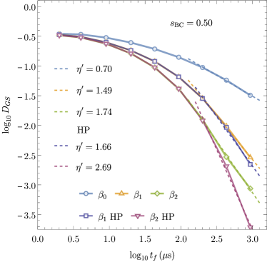
Figure 7: Adiabatic error of AME simulations of the D-Wave programmed BCP and high-precision variants (denoted HP in the legend), for the FM-gadget. Here $s_{\text{BC}}=0.50$, using the schedule of the DW-LN processor and a crosstalk parameter of $0.02$ (see App. G). The adiabatic error is evaluated relative to the Gibbs state ground state probability $\bar{P}_{\text{GS}}^{*}=0.9690$ at $s=0.50$.

IV.3 High precision BCP

To test the effect of the relatively low precision of the implementation of the BCP schedules (using only $12$ interpolation points), we simulated the AME for an additional set of higher-precision constructions of the BC schedule, with $8$ logarithmic partitions up to $s_{\text{BC}}$, rather than the $4$ allotted for the D-Wave schedule (see the construction of App. F). The scaling of the adiabatic error for the FM-gadget is shown in Fig. 7. Since the adiabatic error still appears to have some concavity, the scaling exponents should be interpreted as lower bounds for the asymptotic scaling. We see that the high precision schedule brings the scaling of the adiabatic error significantly closer to the value predicted by the Prop. 1 version of the BCT within anneal times that are currently accessible to D-Wave devices: we find $\eta^{\prime}=1.66,2.69$ for the higher precision schedules, compared to the theoretically expected values of $k+1=2,3$, respectively. The lower precision schedules result in $\eta^{\prime}=1.49,1.74$, respectively. While the values of $\eta^{\prime}$ for the high precision schedules could be refined by simulations at longer anneal times, we do not include them here to avoid floating point error effects. In any case, it would be much more difficult to experimentally verify the adiabatic error to the precision required at longer annealing times. As such, Fig. 7 is likely to be the most practical precision test of boundary cancellation to date on open systems larger than a single qubit.

We also simulated the AME with a precision of $100$ evenly spaced points in the control schedule, to approximate reaching the limit of the analytically exact beta schedule. The results are indiscernible from the high-precision piecewise schedule shown in Fig. 7, indicating that the latter already implements the beta schedule at the smallest precision that is meaningful within the simulated annealing times.

We conclude that the relatively poor agreement with the Prop. 1 BCT predictions we observed in Figure 6(a)-(c), is likely to be improved in future higher precision implementations of the beta schedule.

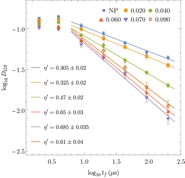
Figure 8: Adiabatic error for a linear anneal of the QAC-encoded FM-gadget with no ramp. Different curves correspond to different values of the penalty strengths, ranging from no penalty (NP; $\lambda=0$) to $\lambda=0.09$ (see symbol legend). The largest slope $\eta^{\prime}=0.69\pm 0.03$ is obtained for $\lambda=0.07$. We directly assumed a linear model with $\bar{P}_{\text{GS}}^{*}=1$ for comparability between the different penalties; performing a non-linear fit first does not change the slopes for $\lambda>0.04$.

IV.4 QAC-Encoded FM Gadget

The scaling of the adiabatic error of the QAC-encoded FM-gadget for various penalty strengths $\lambda$ [recall Eq. (32)] is shown in Fig. 8, for the case of the standard linear control schedule with no ramp. We observe that from the set of values tried, the optimal penalty strength is $\lambda=0.07$. Using this optimal penalty value, the ground state probabilities of BCP with QAC are shown in Fig. 6(d)-6(e). The QAC-protected $P_{\text{GS}}$ results for both $s_{\text{BC}}$ values shown are significantly higher than their unprotected ($\lambda=0$, NP) counterparts in Fig. 6(a)-6(c), consistent with many prior results on the improved performance offered by QAC.

However, we are primarily interested here in QAC’s effect on the BCP. In this regard, at $s_{\text{BC}}=0.45$, there is a notable distinction between different $k$ values, so that QAC amplifies the effect of the BC schedule.

At $s_{\text{BC}}=0.50$, QAC-protected BCP still improves over the linear anneal ($k=0$) by $P_{\text{GS}}$ value, but the improvement is less distinct for different $k$ values. Moreover, $\eta^{\prime}$ is smaller (at most $0.61$) than that for the optimal-$\lambda$ linear QAC anneal in Fig. 8 (for which $\eta^{\prime}=0.69$), signaling that freezing has already mostly occurred before $s=0.50$, and that the optimal $\lambda$ value is $s_{\text{BC}}$-dependent.

Our results demonstrate that the combination of BCP and QAC as error suppression methods is more powerful in terms of the scaling of the adiabatic distance than either method alone: while $k=2$ BCP has $\eta^{\prime}=1.1$ [Fig. 6(a)] and optimal-$\lambda$ linear ($k=0$) QAC has $\eta^{\prime}=0.69$ (Fig. 8), their combination yields $\eta^{\prime}=1.3$ [Fig. 6(d)] and the largest $P_{GS}$ of any other schedule for $t_{f}=12\,\mathrm{\mu s}$.

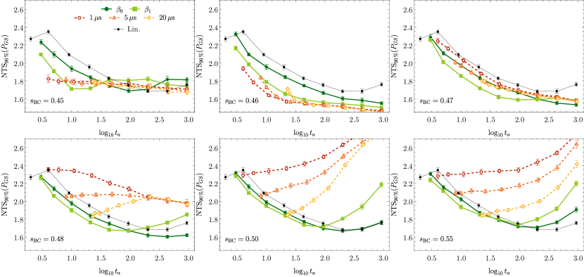
Figure 9: Number of tries to solution for the T-gadget, comparing the pausing protocols (empty symbols) and $\beta_{0},\beta_{1}$ BCP (all with a ramp at $s_{\text{BC}}$), along with the linear anneal without a ramp (denoted “Lin.”; the same data for all panels), for reference. Results shown are for DW-LN, as a function of the total anneal time of each protocol. Different panels have different values of $s_{\text{BC}}$, from $0.45$ to $0.55$. The pausing protocol is shown for different initial anneal times $t_{0}$ of $1$,$5$, and $20\,\mathrm{\mu s}$ (empty symbols), followed by a pause of varying length $t_{p}$ and a $1\,\mathrm{\mu s}$ long ramp (so that the paused portion of the schedule is comparable to BCP). For BCP (filled symbols), $t_{a}=t_{f}+1\mathrm{\mu s}$. For pausing, $t_{a}=t_{0}+t_{p}+1\mathrm{\mu s}$. Both schedules are plotted against $t_{a}$ rather than their natural parameters ($t_{f}$ and $t_{p}$ respectively) for direct comparison.

IV.5 Comparison of the BCP to the Pause-Ramp protocol

A different protocol that attempts to exploit slowing down the anneal is the pausing protocol, which interrupts an ordinary linear anneal by a single pause Marshall et al. (2019); Chen and Lidar (2020); Gonzalez Izquierdo et al. (2021); Albash and Marshall (2021); Izquierdo et al. (2022). Pausing directly uses thermal relaxation at a single point in the anneal to try to increase the ground state probability. As in the BCP, this point should also be after an avoided level crossing, but before the open system dynamics freeze Chen and Lidar (2020).

We compare the BCP to a variant of the usual pausing schedule Marshall et al. (2019) referred to here as the pause-ramp (PR) schedule. While the pausing protocol is typically constructed by interrupting a linear anneal with a pause (but no ramp), PR is constructed by making the first linear segment last for $t_{0}$, pausing for $t_{p}$, and ramping to the end. As with the BCP, we use a ramp that is $1\,\mathrm{\mu s}$ long in all cases. PR is better suited for comparison with BCP than the usual pausing schedule since they differ only in their equilibrium state preparation and not in their behavior during the frozen phase.

As our metric for comparison we use not the ground state probability but rather the number of tries-to-solution (NTS) at a fixed anneal time (with 90% confidence):

$$\mathrm{NTS}_{90\%}(P_{\text{GS}})=\frac{\log(1-0.90)}{\log(1-P_{\text{GS}})}\,$$ (34)

This metric is simply another way to study the ground state probability, interpreted as the expected number of tries needed to find the ground state at least once with 90% confidence, at the given anneal time. We use this rather than the standard time-to-solution (TTS) metric, since the latter requires identifying the optimal anneal time Ronnow et al. (2014); Albash and Lidar (2018); Hen et al. (2015). However, neither the FM-gadget nor the T-gadget exhibited an optimal anneal time in our experiments (not shown).

Figure 9 shows the NTS results for the T-gadget at various values of $s_{\text{BC}}$. It compares the standard schedule (no BCP or pausing), the BCP protocol at $k=0$ and $k=1$, and the PR schedule with different initial anneal and pause times. Starting at $s_{\text{BC}}=0.45$ (top left) the gap is small and thermalization is fast. BCP exhibits two distinct optimal anneal times (minima) for $k=0$ and $k=1$, both of which result in slightly smaller NTS than pausing. Also, the $k=1$ case is optimal at smaller $t_{a}$ than $k=0$, which can be interpreted as as advantage of the higher order protocol. This trend persists for most of the $s_{\text{BC}}$ values shown. Right at $s_{\text{BC}}=0.46$, pausing achieves its optimal NTS curve, with a slight advantage over BCP, and the BCP of each order $k$ is very distinct. However, the advantage of pausing is only present at $s_{\text{BC}}=0.46$, and disappears already at $s_{\text{BC}}=0.47$, showing that pausing performance is highly sensitive to the pause point. Since the BCP slowdown is smooth, the influence of the optimal thermalization at $s_{\text{BC}}=0.46$ remains present, although the distinction between BCP orders diminishes as $s_{\text{BC}}$ grows. Well before $s_{\text{BC}}$ approaches the freeze-out point ($s_{0}\approx 0.51$), pausing becomes detrimental for the T-gadget due to excitations (witnessed by the increase in the NTS metric), while BCP mitigates the excitations until the anneal time becomes too long to avoid them.

These results paint a picture of the two protocols as follows. The relaxation induced by the BCP depends on the properties of the Liouvillian over a neighborhood $(s_{\text{BC}}-\epsilon,s_{\text{BC}}]$. If this neighborhood overlaps with the neighborhood of an avoided level crossing, then the BCP has an opportunity for an advantage, as the speed at which the crossing is traversed is minimized and detrimental excitations to the excited state are reduced. In contrast, PR schedules must try to discontinuously stop the anneal as close as possible to the crossing, and the time required by a paused schedule could be increased due to the longer pause time needed to recover the ground state population, unless the precise optimal pause point is quickly found.

This suggests an important practical point: optimization of the BCP can be simpler than that of PR schedules, by the need to optimize just one discrete parameter $k$ and one continuous parameter $s_{\text{BC}}$. Moreover, $s_{\text{BC}}$ need not be exactly tuned, since even an approximate value can allow the BCP to closely approach its optimal performance. On the other hand, pausing requires $s_{\text{BC}}$ to be optimized very precisely, as well as the anneal and pause times $t_{0}$ and $t_{p}$.

V Discussion and Outlook

We have extended the boundary cancellation theorem for open systems to the case where the Liouvillian gap vanishes at the end of the anneal, and derived the asymptotic scaling of the adiabatic error with the anneal time $t_{f}$. Armed with the corresponding theoretical expectation of the scaling of the adiabatic error for the gapped and gapless cases, we set out to test the scaling predictions and to improve the success probability of quantum annealing hardware by implementing boundary cancelling schedules. The specific functional form of these schedules induces a smooth slowdown in accordance with the boundary cancellation theorem. We experimentally tested boundary cancellation protocols for open systems and evaluated their performance and error-suppression characteristics on specifically designed $8$-qubit gadgets embedded on the DW-LN annealer.

While a quantitative agreement with the theoretical predictions was not observed, we did demonstrate that as long as the protocol terminates before the onset of freezing, it can increase the ground state population in the examples studied here beyond what is achievable with simple linear anneals, and it does so with shorter anneal times. These results are in qualitative agreement with the theoretical scaling predictions of the BCT.

In conjunction with quantum annealing correction (QAC), the boundary cancellation protocol is also capable of improved adiabatic error scaling over what would be achieved with either method alone. While this does not immediately translate to a ground state solution speedup within the annealing problems studied here, we have shown that BCP-QAC is a novel error suppression strategy successfully combining two complimentary methods: the suppression of environmentally induced logical errors and the promotion of relaxation via boundary cancellation.

In contrasting the BCP with the pause-ramp protocol, we found that the BCP is significantly less sensitive to the location of the ramp point, and achieves better performance except at the exact ramp point where the pause-ramp protocol is optimal.

With the small system size of $8$ qubits used in this work, it was possible to collect a large number of annealing samples as well as validate the protocol behavior against the energy spectrum and open system simulations. Future work will assess the protocol for larger system sizes and the impact it has on the scaling of time-to-solution as a function of problem size. The largest expected improvement in the protocol’s performance, based on our simulations, will arise from an increase in the number and resolution of interpolation points along the annealing schedule, which will allow a more faithful experimental implementation of the ideally smooth annealing schedules demanded by the theoretical protocol.

Appendix A Proof of degeneracy when $A(t)=0$

We assume that $A_{i}=\sigma_{i}^{z}$. When $A(t)=0$, $H_{S}\propto H_{Z}$ and commutes with $A_{i}$, so that Eq. (7) yields $A_{i}(\omega)=\sigma_{i}^{z}\delta_{\omega,0}$. Therefore, the dissipator in Eq. (5a) becomes

$$\left.\mathcal{D}\right|_{A(t)=0}=\sum_{ij}\gamma_{ij}(0)\Big{(}\sigma_{j}^{z}\bullet\sigma_{i}^{z}-\frac{1}{2}\left\{\sigma_{i}^{z}\sigma_{j}^{z},\bullet\right\}\Big{)}.$$ (35)

Now let $|n\rangle$ be an eigenstate of $H_{Z}$, where $n=1,\dots,d$ and $d$ is the system’s Hilbert space dimension. Then $|n\rangle\!\langle n|$ commutes with $\sigma_{i}^{z}$, so that $\mathcal{D}\left(|n\rangle\!\langle n|\right)=0$. At the same time, $A_{i}(\omega)=\sigma_{i}^{z}\delta_{\omega,0}$ implies that also the Lamb shift is diagonal in the $\sigma^{z}$ basis. Together with the fact that $|n\rangle\!\langle n|$ also commutes with the system Hamiltonian this implies $\mathcal{L}\left(|n\rangle\!\langle n|\right)=0$, which means that the kernel of $\mathcal{L}$ is at least $d$-dimensional at $A(t_{f})=0$, i.e., that the zero eigenvalue of $\mathcal{L}$ is at least $d$-fold degenerate.

Appendix B Proof of Proposition 4

Here we prove Proposition 4, which concerns the case where the gap closes at the end of the anneal and we enforce boundary cancellation at this point.

We denote by $\mathcal{L}(s)$ the Liouvillian without the BC schedule (i.e., with a linear schedule around $s=1$) while $\mathcal{L}(s(\tau))$ [or $\mathcal{L}(\tau)$ for simplicity] indicates the Liouvillian with the BC schedule. We will use the series developed in Avron et al. (2012) and refined in Campos Venuti and Lidar (2018) together with ideas from (Venuti et al., 2016, App. J). The assumption that $\int_{0}^{1}ds\left\|\mathcal{L}(s)\right\|_{1,1}<\infty$ assures, by Carathéodory’s theorem, that the solution of Eq. (1) exists and is unique in an extended sense Hale (2009), while the requirement that $\mathcal{L}(\tau)$ is $k+2$ differentiable at $k=1$ implies that one can use the series Eq. (43a) below with $\tau=1$ and $N=k$.

By assumption, we have a boundary cancelling schedule at $s=1$. Such a schedule is a function $s=s(\tau)$ where $s(1)=1$ and $s^{(j)}(1)=0$ for $j=1,2,\ldots,k$. That is,

$$s(\tau)=1-g(1-\tau)^{k+1}+O(\delta^{k+2})\ ,\quad\delta\equiv 1-\tau$$ (36)

when $\tau\to 1^{-}$ for some constant $g$. Let

$$\mathcal{L}(s)=\sum_{j=1}\lambda_{j}(s)P_{j}(s)+D(s)$$ (37)

be the instantaneous spectral decomposition of $\mathcal{L}(s)$ (without the BC schedule), i.e., $\lambda_{j}(s)$ are eigenvalues, $P_{j}(s)$ are eigenprojectors, and $D(s)$ is a nilpotent term. We denote by $P(s)$ (without a subscript) the projector related to the zero eigenvalue. The assumption of contractivity implies that $D(s)$ cannot belong to the $\mathcal{L}(s)=0$ subspace. We denote by $\sigma(\tau)$ the unique steady state of $\mathcal{L}(s(\tau))$, i.e., $\mathcal{L}(s(\tau))\sigma(\tau)=0$, $\mathrm{Tr}(\sigma(\tau))=1$ while $\rho(\tau)$ is the solution of Eq. (1) with the BC schedule and with the initial condition $\rho(0)=\sigma(0)$. Note that in the main text $\mathcal{L}(s(\tau))$ is written for simplicity as $\mathcal{L}(\tau)$.

We use a similar approach (and notation) as in Ref. Venuti et al. (2016). Here $\mathcal{E}(\tau)\mathrel{\mathop{\mathchar 58\relax}}=\mathcal{E}(\tau,0)$ is the evolution superoperator satisfying $\partial_{\tau}\mathcal{E}(\tau,\tau^{\prime})=t_{f}\mathcal{L}(s(\tau))\mathcal{E}(\tau,\tau^{\prime})$ and $\mathcal{E}(\tau_{3},\tau_{2})\mathcal{E}(\tau_{2},\tau_{1})=\mathcal{E}(\tau_{3},\tau_{1})$ together with $\mathcal{E}(\tau,\tau)=\leavevmode{\rm 1\mkern-4.8muI}$, i.e.,

$$\mathcal{E}(\tau_{2},\tau_{1})=\mathcal{E}^{-1}(\tau_{3},\tau_{2})\mathcal{E}(\tau_{3},\tau_{1}).$$ (38)

Let $V(\tau)$ be the adiabatic intertwiner as defined in Venuti et al. (2016) and, following the same notation therein, $W(\tau)\mathrel{\mathop{\mathchar 58\relax}}=P(\tau)V(\tau)=V(\tau)P(0)$. We start with Eq. (D4) of Ref. Venuti et al. (2016) which we reproduce here for clarity:

$$\left[\mathcal{E}^{-1}(\tau)V(\tau)-\leavevmode{\rm 1\mkern-4.8muI}\right]P(0)=\int_{0}^{\tau}\mathcal{E}^{-1}(\tau_{1})\dot{W}(\tau_{1})d\tau_{1},$$ (39)

where the dot denotes differentiation with respect to the argument of the corresponding operator. Hence

$$\left[\mathcal{E}^{-1}(1)V(1)-\leavevmode{\rm 1\mkern-4.8muI}\right]P(0)=\left(\int_{0}^{\tau}+\int_{\tau}^{1}\right)\mathcal{E}^{-1}(\tau_{1})\dot{W}(\tau_{1})d\tau_{1}$$ (40a)

$$\quad=\left(\mathcal{E}^{-1}(\tau)V(\tau)-\leavevmode{\rm 1\mkern-4.8muI}\right)P(0)+\int_{\tau}^{1}\mathcal{E}^{-1}(\tau_{1})\dot{W}(\tau_{1})d\tau_{1},$$ (40b)

Now apply $\mathcal{E}(1)\mathrel{\mathop{\mathchar 58\relax}}=\mathcal{E}(1,0)$ from the left and use Eq. (38) repeatedly, to obtain:

$$\left(V(1)-\mathcal{E}(1)\right)P(0)=\left(\mathcal{E}(1,\tau)V(\tau)-\mathcal{E}(1,0)\right)P(0)$$

$$\qquad+\int_{\tau}^{1}\mathcal{E}(1,\tau_{1})\dot{W}(\tau_{1})d\tau_{1}$$ (41a)

$$\quad=\mathcal{E}(1,\tau)\left(V(\tau)-\mathcal{E}(\tau)\right)P(0)+\int_{\tau}^{1}\mathcal{E}(1,\tau_{1})\dot{W}(\tau_{1})d\tau_{1}.$$ (41b)

Now apply $\sigma(0)$ from the right. Note that $V(\tau)$ is continuous, being the solution of a differential equation. So $V(1)P(0)\sigma(0)=\lim_{\tau\to 1^{-}}\sigma(\tau)=\sigma(1^{-})$ and we obtain finally

$$\sigma(1^{-})-\rho(1) =\mathcal{E}(1,\tau)\left(\sigma(\tau)-\rho(\tau)\right)$$

$$\qquad+\int_{\tau}^{1}\mathcal{E}(1,\tau_{1})\dot{W}(\tau_{1})\sigma(0)d\tau_{1}.$$ (42)

Eq. (42) is the starting point of our analysis. Since in Eq. (42) $\tau<1$ and the system is gapped in $\left[0,\tau\right]$, we can use the result of Campos Venuti and Lidar (2018) to obtain the behavior of $\sigma(\tau)-\rho(\tau)$. Assuming that $\mathcal{L}(\tau)$ is at least $N+2$ times differentiable in a neighborhood of $\tau=1$, one has the following series Campos Venuti and Lidar (2018) with $\epsilon=1/t_{f}$ for $\tau$ in the same neighborhood:

$$\rho(\tau) =\sigma(\tau)+\sum_{n=1}^{N}\epsilon^{n}b_{n}(\tau)+\epsilon^{N+1}r_{N}(\epsilon,\tau)$$ (43a)

$$b_{1}(\tau) =S(\tau)\dot{P}(\tau)\sigma(\tau)=S(\tau)\dot{\sigma}(\tau)$$ (43b)

$$b_{n+1}(\tau) =S(\tau)\dot{b}_{n}(\tau),\quad n=1,2,\ldots,N$$ (43c)

where the remainder is

$$r_{N}(\epsilon,\tau)=b_{N+1}(\tau)-\mathcal{E}(\tau)b_{N+1}(0)\\ \quad-\int_{0}^{\tau}\mathcal{E}(\tau,\tau^{\prime})\dot{b}_{N+1}(\tau^{\prime})d\tau^{\prime}$$ (44)

and $S(\tau)$ is the reduced resolvent, defined as:

$$S(\tau)\mathrel{\mathop{\mathchar 58\relax}}=\lim_{z\to 0}\left(\leavevmode{\rm 1\mkern-4.8muI}-P(\tau)\right)\left(\mathcal{L}(\tau)-z\right)^{-1}\left(\leavevmode{\rm 1\mkern-4.8muI}-P(r)\right).$$ (45)

We will keep $N$ free and only fix it at the end when needed. The series (43a) cannot be used at $\tau=1$, because the assumption of a gapped Liouvillian does not hold there. Hence we must keep $\tau<1$ but investigate the kind of divergences that arise when $\tau\to 1^{-}$.

The other assumption is that, without the BC schedule, the Liouvillian gap closes at $s=1$ in such a way that $\lambda_{1}(s)\simeq v(1-s)^{\alpha}$ as $s\to 1^{-}$. Therefore, using Eqs. (36) and (37), close to $s=1$ the Liouvillian with the BC schedule behaves as

$$\mathcal{L}(s(\tau))\simeq\tilde{v}(1-\tau)^{\tilde{\alpha}}P_{1}(s(\tau))$$

$$\qquad+\sum_{j>1}\lambda_{j}(s(\tau))P_{j}(s(\tau))+D(s(\tau)),$$ (46)

with $\tilde{v}=vg^{\alpha}$ and $\tilde{\alpha}=\alpha(k+1)$. Accordingly, the most diverging term of the reduced resolvent $S(\tau)$ behaves as

$$S(\tau)\sim\frac{P_{1}}{\delta^{\tilde{\alpha}}},$$ (47)

where henceforth we do not always explicitly emphasize the dependence on $\tau$ when it does not lead to a divergence. Now, the derivatives of the projectors behave as

$$\partial_{\tau}P_{j}(s(\tau)) =\partial_{s}P_{j}(s)\partial_{\tau}s(\tau)\sim\partial_{s}P_{j}\delta^{k}.$$ (48)

Hence, we see that when $\tau\to 1^{-}$, $b_{1}$ diverges as

$$b_{1}(\tau)\sim\frac{1}{\delta^{\tilde{\alpha}-k}}.$$ (49)

When we construct $b_{n}$ according to Eq. (43c), at each iteration we gain a derivative and a factor of $S$. Thus, defining $\beta_{n}$ via $b_{n}(\tau)\sim\delta^{-\beta_{n}}$, we obtain $\beta_{n+1}=\beta_{n}+\tilde{\alpha}+1$. This has the solution

$$\beta_{n} =n\left(\tilde{\alpha}+1\right)-k-1$$ (50a)

$$=n\left(\alpha k+\alpha+1\right)-k-1.$$ (50b)

Hence, we can find positive constants $A_{n}$ such that

$$\left\|b_{n}(\tau)\right\|_{1}\leq\frac{A_{n}}{\delta^{\beta_{n}}}.$$ (51)

Turning to the remainder, we take the trace norm of Eq. (44) and use the triangle inequality:

$$\|r_{N}(\epsilon,\tau)\|_{1} \leq\|b_{N+1}(\tau)\|_{1}+\|\mathcal{E}(\tau)b_{N+1}(0)\|_{1}$$

$$\quad+\int_{0}^{\tau}\|\mathcal{E}(\tau,\tau^{\prime})\dot{b}_{N+1}(\tau^{\prime})\|_{1}d\tau^{\prime}.$$ (52)

Next, we use $\left\|\mathcal{E}x\right\|_{1}\leq\left\|\mathcal{E}\right\|_{1,1}\left\|x\right\|_{1}$ for a superoperator $\mathcal{E}$ and operator $x$, and the fact that since $\mathcal{E}(\tau_{2},\tau_{1})$ is a completely positive trace preserving map for $\tau_{2}\geq\tau_{1}$, we have

$$\left\|\mathcal{E}(\tau_{2},\tau_{1})\right\|_{1,1}=1\ ,\quad\tau_{2}\geq\tau_{1}.$$ (53)

Therefore

$$\int_{0}^{\tau}\|\mathcal{E}(\tau,\tau^{\prime})\dot{b}_{N+1}(\tau^{\prime})\|_{1}d\tau^{\prime}\leq\int_{0}^{\tau}\|\dot{b}_{N+1}(\tau^{\prime})\|_{1}d\tau^{\prime}.$$ (54)

Now using $b_{n}(\tau)\sim\delta^{-\beta_{n}}$ again we obtain $\|\dot{b}_{N+1}(\tau^{\prime})\|_{1}\sim(1-\tau^{\prime})^{-\beta_{N+1}-1}$, which integrated from $0$ to $\tau$ implies that

$$\int_{0}^{\tau}\|\mathcal{E}(\tau,\tau^{\prime})\dot{b}_{N+1}(\tau^{\prime})\|_{1}d\tau^{\prime}\leq\frac{B}{\delta^{\beta_{N+1}}},$$ (55)

for some positive constant $B$. All in all, we obtain for the remainder

$$\left\|r_{N}(\epsilon,\tau)\right\|\leq\frac{A_{N+1}}{\delta^{\beta_{N+1}}}+\left\|b_{N+1}(0)\right\|+\frac{B}{\delta^{\beta_{N+1}}},$$ (56)

Here $\left\|b_{N+1}(0)\right\|$ is just another constant, independent of $\delta$. Combining these results we obtain from Eq. (43a), after redefining the constants:

$$\left\|\rho(\tau)-\sigma(\tau)\right\|\leq\sum_{n=1}^{N+1}\epsilon^{n}\frac{A_{n}}{\delta^{\beta_{n}}}+\epsilon^{N+1}A_{N+2}.$$ (57)

It remains to estimate the second term on the RHS of (42). Using the mean value theorem, $\dot{W}=\dot{P}W$ (Venuti et al., 2016, Eq. (C1)), and $W(\tau)\sigma(0)=\sigma(\tau)$, we have:

$$\int_{\tau}^{1}\mathcal{E}(1,\tau_{1})\dot{W}(\tau_{1})\sigma(0)d\tau_{1} =\delta\mathcal{E}(1,\tilde{\tau})\dot{P}(\tilde{\tau})\sigma(\tilde{\tau}),$$ (58)

where $\tilde{\tau}\in\left[\tau,1\right]$, and we used $\delta=1-\tau$. Hence, when taking the norm of Eq. (58), using Eqs. (48) and (53), we obtain, for some positive constant $C$:

$$\left\|\int_{\tau}^{1}\mathcal{E}(1,\tau_{1})\dot{W}(\tau_{1})\sigma(0)d\tau_{1}\right\|\leq C\delta^{k+1}.$$ (59)

Using Eqs. (57) and (59), we finally obtain after taking the norm of Eq. (42):

$$\left\|\rho(1)-\sigma(1^{-})\right\| \leq\sum_{n=1}^{N+1}\epsilon^{n}\frac{A_{n}}{\delta^{\beta_{n}}}+\epsilon^{N+1}A_{N+2}+C\delta^{k+1}$$ (60)

$$=\mathrel{\mathop{\mathchar 58\relax}}f(\delta,\epsilon).$$

In this derivation $\tau=1-\delta$ is sufficiently close to one but otherwise free. Thus, we can now minimize $f$ as a function of $\delta$. Differentiating $f$ we obtain:

$$\partial_{\delta}f =-\sum_{n=1}^{N+1}\epsilon^{n}\frac{\beta_{n}A_{n}}{\delta^{\beta_{n}+1}}+(k+1)C\delta^{k}=0$$ (61a)

$$\hookrightarrow\delta^{-k}\partial_{\delta}f =-\sum_{n=1}^{N+1}\epsilon^{n}\frac{\beta_{n}A_{n}}{\delta^{n\left(\alpha k+\alpha+1\right)}}+(k+1)C=0.$$ (61b)

We now make the ansatz $\delta=\nu\epsilon^{\gamma}$. We wish to find a $\gamma$ such that the solution $\nu$ of Eq. (61b) does not depend on $\epsilon$. This is satisfied if all the summands in Eq. (61b) do not scale with $\epsilon$, i.e., are constant, which holds for $n-\gamma n\left(\alpha k+\alpha+1\right)=0$. This means that $\gamma=1/\left(\alpha k+\alpha+1\right)$. The value of $\nu$ can be found by solving

$$\sum_{n=1}^{N+1}\frac{\beta_{n}A_{n}}{\nu^{n\left(\alpha k+\alpha+1\right)}}=(k+1)C.$$ (62)

Picking $N=1$ in Eq. (62) one can show that the resulting quadratic equation in $x\mathrel{\mathop{\mathchar 58\relax}}=\nu^{-(\alpha k+\alpha+1)}$ always has a positive solution, which means that Eq. (62) always has a real solution $\nu$.

Substituting $\delta=\nu\epsilon^{\gamma}$ with $\gamma=1/\left(\alpha k+\alpha+1\right)$ into Eq. (60), we see that all terms scale as $\epsilon^{\eta}$ with the exponent

$$\eta=\frac{k+1}{\alpha k+\alpha+1}.$$ (63)

In other words:

$$\left\|\rho(1)-\sigma(1^{-})\right\|\leq C^{\prime}\epsilon^{\eta},$$ (64)

as reported in the main text. See Figure 10 for numerical simulations confirming Eqs. (63) and (64).

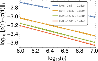
Figure 10: Test of the bound given in Proposition 4, for the case of a single qubit subject to evolution under the AME. The Hamiltonian is $H(\tau)=\omega_{x}(1-\beta_{k}(\tau))\sigma^{x}+\omega_{z}\beta_{k}(\tau)\sigma^{z}$ with BC schedule $\beta_{k}(\tau)=\mathrm{B}_{\tau}(1,k+1)/\mathrm{B}_{1}(1,k+1)$ [$\mathrm{B}$ is the incomplete beta function, Eq. (31)] which has $k$ vanishing derivatives at $\tau=1$ and is linear at $\tau=0$. The system-bath coupling is via $\sigma^{z}$, which assures that the Liouvillian is gapless at $\tau=1$ with a gap-closing exponent $\alpha=2$ Venuti et al. (2016). The bath spectral density is Ohmic [Eq. (11)]; the parameters are $g=1,\,\beta=1,$ $\omega_{x}=\omega_{z}=-1/2$ in arbitrary units. Dots are results of solving for the evolution while the continuous lines are linear fits. The theoretical expectation given by Eq. (63) is $\eta=\{0.333,\,0.4,\,0.428,\,0.444\}$ for $k=\{0,1,2,3\}$, respectively, and is an excellent agreement with the the last column of the legend (obtained via a linear fit).

Appendix C Gap closing in the middle: Numerical check

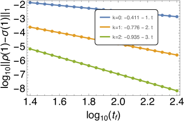
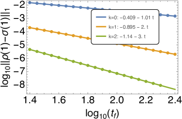
Figure 11: Numerical simulations for the case where the Liouvillian gap closes in the middle of the evolution and one performs BC at the end. Results are for the single qubit AME with the Hamiltonians given in (a) Eq. (65a) and (b) Eq. (66a). The bath spectral density is Ohmic [Eq. (11)] and the parameters are $g=1,\,\beta=1,$ in arbitrary units. Dots are results of solving for the evolution while the continuous lines are linear fits. The fits are in an excellent agreement with $\eta=k+1$, as shown by the the last column of the two legends.

Here we present numerical simulations for the case where the Liouvillian gap closes in the middle of the evolution and one performs boundary cancellation at the end, as discussed in Sec. II.3 of the main text.

We first consider the following Hamiltonian:

$$H(\tau) =\sigma^{y}+(\tau-1)^{k+1}X+\left(\tau-1\right)^{k+2}Y$$ (65a)

$$X\mathrel{\mathop{\mathchar 58\relax}}= \left(-1\right)^{k}\left[\sigma^{x}-2^{k+2}\sigma^{z}+\left(2^{k+2}-1\right)\sigma^{y}\right]$$ (65b)

$$Y\mathrel{\mathop{\mathchar 58\relax}}= 2\left(-1\right)^{k}\left[\sigma^{x}-2^{k+1}\sigma^{z}+\left(2^{k+1}-1\right)\sigma^{y}\right].$$ (65c)

One can check that $H\left(0\right)=\sigma^{x}$, $H\left(1/2\right)=\sigma^{z}$, $H(1)=\sigma^{y}$ and that the first $k$ derivatives of $H(\tau)$ at $\tau=1$ are zero. Hence the Liouvillian gap closes with exponent $\alpha=2$ at $\tau=1/2$ and there is a BC schedule at the end. Numerical results confirming the expected scaling $\eta=k+1$ are presented in Fig. 11.

Another possibility is to use the following Hamiltonian, which performs the traditional interpolation from a transverse to a longitudinal field:

$$H\left(\tau\right) =s\left(\tau\right)\sigma^{x}+\left[1-s\left(\tau\right)\right]\sigma^{z}$$ (66a)

$$s(\tau) \mathrel{\mathop{\mathchar 58\relax}}=\left(2\left(2\frac{\mathrm{B}_{(1+\tau)/2}(1,k+1)}{\mathrm{B}_{1}(1,k+1)}-1\right)-1\right)^{2}.$$ (66b)

The schedule in Eq. (66b) starts with $\sigma^{x}$ at $s(0)=1$ and ends with $\sigma^{z}$ at $s(1)=1$, where it has $k$ vanishing derivatives. The Liouvillian gap closes with $\alpha=4$ at some point $s^{*}_{k}$. Numerical results again confirm the expected scaling $\eta=k+1$, as shown in Fig. 11.

All our numerical results (we have also performed numerics for up to 4 qubit Hamiltonians, not shown here) predict the following scaling for the adiabatic error in this setting:

$$\left\|\rho(1)-\sigma(1)\right\|_{1} \leq\frac{C}{t_{f}^{\eta}}\ ,$$ (67a)

$$\mathrm{with\,\,} \eta=k+1\ .$$ (67b)

In other words, the adiabatic error is insensitive to the closing of the gap in the middle of the evolution. Note that this result is different from the analogous one in the closed system setting where the adiabatic error scales with an exponent $\eta=1/(\alpha+1)$, where $\alpha$ in this case is the exponent that determines the closing of the Hamiltonian (not Liouvillian) gap.

Appendix D Proof that $\langle 0|\sigma_{j}^{z}|n\rangle=O\left(A^{q}\right)$

In the main text we stated that $\langle 0|\sigma_{j}^{z}|n\rangle=O\left(A^{q}\right)$, and hence that the transition matrix elements $W_{0n}=O\left(A^{2q}\right)$ are suppressed for $n\geq 1$. Generalizing beyond the scenario in the main text, we now allow for degeneracy in the eigenstates of $H_{Z}$.

We assume the transverse field is not zero and investigate the behavior of the rates when $A\to 0$. For this value of $A(t)\neq 0$, let $H_{S}=\sum_{n}E_{n}\tilde{P}_{n}$ be the spectral decomposition of the system Hamiltonian, where $\tilde{P}_{n}$ are the (possibly degenerate) spectral projectors. The Bohr frequencies have the form $\omega=E_{b}-E_{a}$ and we can label the jump operators $A_{j}(\omega)$ as

$$A_{ab,j}(t)=\tilde{P}_{a}(t)\sigma_{j}^{z}\tilde{P}_{b}(t).$$ (68)

We omit the time dependence from here on.

Let us consider the operators $A_{ab,j}$ perturbatively around $A(t)=0$. We denote by $P_{a}$ the (unperturbed) spectral projectors at $A(t)=0$, which are diagonal in the computational basis. By assumption, the degeneracy of $\tilde{P}_{a}$ does not change along the anneal, so that the $\tilde{P}_{a}$ are smoothly connected with the $P_{a}$. We use the Kato perturbation theory formalism Kato (1995), and denote the perturbation by $V\mathrel{\mathop{\mathchar 58\relax}}=H_{X}$. Moreover, for level $a$, we define the reduced resolvent as

$$R_{a}=\sum_{n\neq a}\frac{P_{n}}{E_{n}-E_{a}}.$$ (69)

For fixed $a\neq b$ we expand the jump operators in powers of the transverse field:

$$A_{ab,j}=\tilde{P}_{a}\sigma_{j}^{z}\tilde{P}_{b}\mathrel{\mathop{\mathchar 58\relax}}=\sum_{n=0}A^{n}C_{n}.$$ (70)

At zeroth order we have (since $a\neq b$)

$$C_{0}=P_{a}\sigma_{j}^{z}P_{b}=P_{a}P_{b}\sigma_{j}^{z}=0.$$ (71)

At first order, perturbation theory gives

$$C_{1} =-P_{a}\sigma_{j}^{z}\left(P_{b}VR_{b}+R_{b}VP_{b}\right)$$

$$\qquad-\left(P_{a}VR_{a}+R_{a}VP_{a}\right)\sigma_{j}^{z}P_{b}$$ (72a)

$$=-P_{a}\sigma_{j}^{z}R_{b}VP_{b}-P_{a}VR_{a}\sigma_{j}^{z}P_{b}$$ (72b)

$$=-\sigma_{j}^{z}R_{b}P_{a}VP_{b}-P_{a}VP_{b}R_{a}\sigma_{j}^{z}\,.$$ (72c)

Now recall that $V=H_{X}=2S_{x}=(S_{+}+S_{-})$ where $S_{x}$ ($S_{\pm}$) is the total spin-$x$ operator (ladder operator) and hence $V$ changes the Hamming distance by one. As a consequence, $P_{a}VP_{b}=0$ if $\text{HD}(a,b)\neq 1$ where we denoted by $\text{HD}(a,b)$ the smallest Hamming distance among the representative states of the projectors $P_{a}$ and $P_{b}$. I.e., if $P_{a}=\sum_{\mu=1}^{d_{a}}|\mu a\rangle\langle\mu a|$, $P_{b}=\sum_{\nu=1}^{d_{b}}|\nu b\rangle\langle\nu b|$ for some Ising states $|\mu a\rangle,\,|\nu b\rangle$,

$$\text{HD}(a,b)\mathrel{\mathop{\mathchar 58\relax}}=\min_{\mu,\nu}\text{HD}\left(|\mu a\rangle,|\nu b\rangle\right).$$ (73)

At second order we obtain

$$C_{2} =\left(P_{a}VR_{a}+R_{a}VP_{a}\right)\sigma_{j}^{z}\left(P_{b}VR_{b}+R_{b}VP_{b}\right)+$$

$$P_{a}\sigma_{j}^{z}\left(R_{b}VP_{b}VR_{b}+R_{b}VR_{b}VP_{b}-R_{b}^{2}VP_{b}VP_{b}\right)+$$

$$\left(P_{a}VR_{a}VR_{a}+R_{a}VP_{a}VR_{a}-P_{a}VP_{a}VR_{a}^{2}\right)\sigma_{j}^{z}P_{b}\,.$$ (74)

The formulas become increasingly complicated, but we see that at order $k$, $C_{k}$ is sum of terms of the form $O_{z}^{(1)}VO_{z}^{(2)}\cdots VO_{z}^{(k+1)}$ where there are $k$ $V$’s and we denote by $O_{z}^{(j)}$ any operator diagonal in the same basis as $\sigma^{z}$. Two of the $O_{z}^{(i)}$ ($i=1,2,\ldots,k+1$) comprise $P_{a}$ and $P_{b}$. Let $d_{s}$ be the number of $V$’s sandwiched between $P_{a}$ and $P_{b}$. Then this term is zero if $\text{HD}(a,b)>d_{s}$. Since at order $k$, $d_{s}$ is necessarily $\leq k$, we see that $C_{k}$ is zero if $\text{HD}(a,b)>k$. Alternatively, note that the effect of each $O_{z}^{(j)}$ on computational basis states is simply that of creating a multiplicative constant but otherwise it leaves computational basis states unchanged. So, apart from a multiplicative constant each term in $C_{k}$ has the form $|\mu a\rangle\langle\mu a|V^{d_{s}}|\nu b\rangle\langle\nu b|$. Summarizing, if $\text{HD}(a,b)=q$, $A_{ab,j}=O\left(A^{q}\right).$ Since in the Pauli matrix $W_{ab}$ there appear two Lindblad operators per Bohr frequency ($a,b$ pair) we have just shown that $W_{ab}=O\left(A^{2q}\right)$. In particular, this is true if the level $a=0$ and $b=n$ are non-degenerate as it is the case in the main text.

Figure 12 shows that this prediction is borne out in numerical simulations.

Figure 12: The transition matrix elements $W_{0n}$ of the FM-gadget for $n=1,2,3$ (solid), for which $q=8,7,6$, respectively, as a function of $A$, along with $A^{2q}$ shifted to most closely align with the $W_{0n}(A)$ curves (dashed). The agreement is clearly visible for sufficiently small $A$. The transverse field schedule used is $A(s)={30\,\mathrm{ns}^{-1}}(1-s)$ while $B(s)={10\,\mathrm{ns}^{-1}}$ is held constant. This allows the scaling to be seen clearly for small $A$ without changing the overall energy scale of the Hamiltonian.

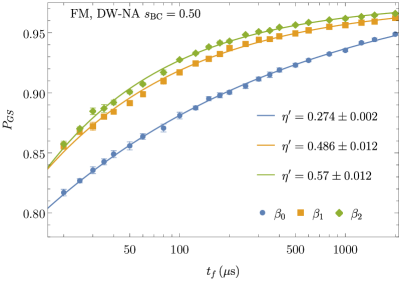
(a)  

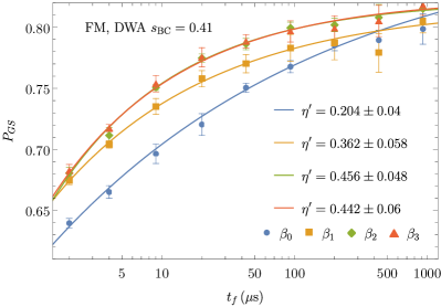
(b)  

Figure 13: Ground state probabilities and fits for the BCP applied to the FM gadget using (a) DW2KQ at NASA QuAIL and (b) D-Wave Advantage at the appropriate values of $s_{\text{BC}}$ where the fits are most distinguishable.

Appendix E Determination of the Freezing Point

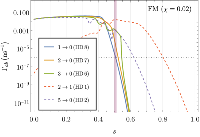
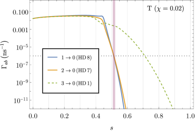
Figure 14: Thermal transition rates of the adiabatic master equation (with $\eta_{0}g^{2}=5.0\times 10^{-4}$ ) for some pairs of energy eigenstates $a\to b$ as the DW-LN schedule progresses linearly for the FM-gadget (top) and the T-gadget (bottom). The horizontal dotted line denotes the rate $1/t_{f}$, which is on the order of magnitude of the smallest rate that can be reliably observed within an anneal time of $t_{f}=10^{3}\,\mathrm{\mu s}$. Below this line, thermal relaxation events rapidly become extremely rare, hence the onset of frozen dynamics during the anneal. The Hamming distances between the final computational states corresponding to the eigenstate transitions are also listed. When an excited state is only a small Hamming distance away from the ground state, the transition freezes later in the anneal since only a much smaller number of qubits need to tunnel through. This is the case for the $2\to 1$ and $3\to 1$ transitions in the FM-gadget, and the $3\to 0$ transition in the T-gadget.

The resulting transition rates between energy eigenstates in the AME are shown in Fig. 14 for both the FM and the T-gadgets. Since the magnitude of available annealing times are limited to $10^{3}\,\mathrm{\mu s}$, we expect that a transition will become too rare to observe once it drops below $1/t_{f}\approx 10^{-6}$ GHz. With the majority of the population in the ground state and first excited state, we therefore expect freezing to occur when $\Gamma_{10}$ goes below this value. This intersection determines the freeze-out points highlighted in Fig. 4.

Appendix F Schedule Construction

The annealing schedule of the DW-LN used in our main experiments is shown in Fig. 1. All simulations are based on this schedule and its operating temperature at the time of sample collection (13.5 $\mathrm{mK}$).

First, suppose $s^{*}(\tau)=\beta_{k}(\tau)$ is a beta-schedule terminating at $s=1$ and let $\tau^{*}(s)$ denote its inverse function. The construction of a piecewise-linear approximation to $s^{*}(\tau)$ is as follows:

1. The initial point $(\tau_{0},s_{0})=(0,0)$ and the final point $(\tau_{10},s_{10})=(1,1)$.

2. A separation point $(\tau_{5},s_{5})=(\tau^{*}(s_{c}),s_{c})$ for some choice of $s_{c}$.

3. Linearly partition $s_{1},\ldots s_{4}$, i.e., assign $s_{j}=js_{c}/5$ and set $\tau_{j}=\tau^{*}(s_{j})$ for $j=1\ldots 4$.

4. Logarithmically partition $s_{6},\ldots,s_{9}$ between $s_{c}$ and $1$, i.e., assign $s_{j+1}=1-(1-s_{j})/2$) and set $\tau_{j}=\tau^{*}(s_{j})$ for $j=6\ldots 9$.

Thus, for a schedule that terminates at the ramp point $s_{\text{BC}}$, we have the following $12$-point scheme:

1. Construct the first $11$ points according to the above procedure, and then rescale each $s_{j}\to s_{\text{BC}}s_{j}$.

2. The final $12$th point is $(\tau_{11},s_{11})=(\tau_{10}+\delta,1)$, where $\delta$ is constrained by the maximum ramp slope of the hardware, i.e., $\delta=1\mu\textrm{s}/t_{f}$.

Note that when the ramp is included $s=1$ corresponds to $\tau=1+\delta$ and $s_{\text{BC}}<1$. Aside from the order $k$, there are the three annealing parameters $s_{c},s_{\text{BC}},$ and $t_{f}$ that must be specified for the protocol. We took $s_{c}=0.9$ for the construction of the beta schedules.

Adjusting the $s_{c}$ parameter to $0.95$ to improve the precision of the analytic behavior of the beta schedule did not have a substantial effect on the ground state probabilities of the empirical D-Wave results. It is likely that such a precision exceeds what can be reliably and repeatedly implemented on the hardware.

Appendix G Crosstalk

It is known that, due to the difficulty of hardware fabrication of the D-Wave processors, programming the couplings and field to have certain values induces non-zero fields and couplings also on other links of the graph, despite designs meant to minimize such crosstalk Harris et al. (2009). We use the ferromagnetic crosstalk model defined by the following transformations Albash et al. (2015a):

$$h_{i} \mapsto h_{i}-\chi\sum_{k\neq i}J_{ik}h_{k}$$ (75a)

$$J_{ij} \mapsto J_{ij}+\chi\sum_{k\neq i,j}J_{ik}J_{jk}$$ (75b)

where $\chi$ is the crosstalk strength. We assume a strength of $\chi=0.02$ throughout. We have checked that optimizing the value of $\chi$ further does not substantially affect our numerical results. This crosstalk has the effect of breaking the degeneracy of the first and second excited states shown in Fig. 4.

We note that the transformation (75) commutes with gauge (or spin-reversal) transformations of the Hamiltonian Boixo et al. (2013); Job and Lidar (2018), so population shifts due to crosstalk do not depend on the gauge.

Appendix H Data Collection and Fitting

The probabilities at a given anneal time are obtained from a sample of 20 submissions (10 for QAC), where each submission programs 5 random global gauges of the gadget repeated over 31 unit cells, and samples each gauge 200 times (see Ref. Job and Lidar (2018) for a review of the gauging procedure and other best practices). To mitigate time-fluctuating systematic biases, submissions for the same anneal time are not consecutively submitted (anneal times are cycled for every schedule). Estimates for the ground state probability are taken from the average of the ground state probabilities of the 20 submissions. Error bars for each measured ground state probabilities are derived from twice the standard deviation over all submissions. Either by non-linear fits on the transformed data, or by linear fits on the log-log transformed data assuming a fixed $\bar{P}_{\text{GS}}^{*}$, we find the constant $C$ and exponent $\eta$ such that the $\chi^{2}$ with $D_{\mathrm{\text{GS}}}$ is minimized. Nonlinear fits are performed as a function of $1/t_{f}$. The estimates of $\eta^{\prime}$ for the D-Wave data are obtained by performing fits on 100 bootstrap samples of the collected ground state probabilities. We use the median values of the parameter distributions as the estimators for the parameters as they are robust to the outliers in bootstrapping that occur. The error estimate is derived from half of the range of the 90% confidence interval of the parameter distribution. The non-linear fits are evaluated using the Mathematica function NonlinearModelFit with the method NMinimize(NelderMead). The non-linear $\chi^{2}$ objective was weighed by the variances of the ground state probabilities.

Appendix I Results for alternative D-Wave QPUs

We performed similar BCP quantum annealing experiments with the DW2KQ at NASA QuAIL (DW-NA) and with the D-Wave Advantage (DWA) annealers, while the main results used the low-noise DW2KQ processor through D-Wave Leap (DW-LN) The scaling behavior of the ground state probabilities at appropriate values of $s_{\text{BC}}$ is shown in Fig. 13. These results should be contrasted with Fig. 6(a), for the DW-LN. All three QPUs have different schedules and thermal properties that affect the qualitative behavior of the BCP, so it is difficult to make a direct comparison between the devices. However, $\eta$ is generally larger in DW-LN compared to either DW-NA or DWA when $s_{\text{BC}}$ is in the appropriate region for each annealer. Furthermore, DWA appears to exhibit more significant time-dependent deviations, as can be noted in the $\beta_{2}$ schedule at $t_{f}=431$ in Fig. 13.

References

- Farhi et al. (2000) E. Farhi, J. Goldstone, S. Gutmann, and M. Sipser, arXiv:quant-ph/0001106 (2000), arXiv:quant-ph/0001106 .
- Kadowaki and Nishimori (1998) T. Kadowaki and H. Nishimori, Physical Review E 58, 5355 (1998).
- Amin et al. (2018) M. H. Amin, E. Andriyash, J. Rolfe, B. Kulchytskyy, and R. Melko, Physical Review X 8, 021050 (2018).
- Kato (1950) T. Kato, Journal of the Physical Society of Japan 5, 435 (1950).
- Jansen et al. (2007) S. Jansen, M.-B. Ruskai, and R. Seiler, Journal of Mathematical Physics 48, 102111 (2007).
- Joye (2007) A. Joye, Commun. Math. Phys. 275, 139 (2007).
- Garrido and Sancho (1962) L. M. Garrido and F. J. Sancho, Physica 28, 553 (1962).
- Nenciu (1993) G. Nenciu, Commun. Math. Phys. 152, 479 (1993).
- Hagedorn and Joye (2002) G. A. Hagedorn and A. Joye, Journal of Mathematical Analysis and Applications 267, 235 (2002).
- Lidar et al. (2009) D. A. Lidar, A. T. Rezakhani, and A. Hamma, Journal of Mathematical Physics 50, 102106 (2009).
- Wiebe and Babcock (2012) N. Wiebe and N. S. Babcock, New Journal of Physics 14, 013024 (2012).
- Ge et al. (2016) Y. Ge, A. Molnár, and J. I. Cirac, Physical Review Letters 116, 080503 (2016).
- Campos Venuti and Lidar (2018) L. Campos Venuti and D. A. Lidar, Physical Review A 98, 022315 (2018).
- Albash and Lidar (2015) T. Albash and D. A. Lidar, Physical Review A 91, 062320 (2015).
- Lidar (2019a) D. A. Lidar, Physical Review A 100, 022326 (2019a).
- Johnson et al. (2011) M. W. Johnson, M. H. S. Amin, S. Gildert, T. Lanting, F. Hamze, N. Dickson, R. Harris, A. J. Berkley, J. Johansson, P. Bunyk, E. M. Chapple, C. Enderud, J. P. Hilton, K. Karimi, E. Ladizinsky, N. Ladizinsky, T. Oh, I. Perminov, C. Rich, M. C. Thom, E. Tolkacheva, C. J. S. Truncik, S. Uchaikin, J. Wang, B. Wilson, and G. Rose, Nature 473, 194 (2011).
- D-Wave Systems Inc. (2018) D-Wave Systems Inc., “The D-Wave 2000Q Quantum Computer Technology Overview,” (2018).
- Albash et al. (2012) T. Albash, S. Boixo, D. A. Lidar, and P. Zanardi, New Journal of Physics 14, 123016 (2012).
- Davies (1974) E. B. Davies, Comm. Math. Phys. 39, 91 (1974).
- Albash et al. (2015a) T. Albash, W. Vinci, A. Mishra, P. A. Warburton, and D. A. Lidar, Physical Review A 91, 042314 (2015a).
- Albash et al. (2015b) T. Albash, I. Hen, F. M. Spedalieri, and D. A. Lidar, Physical Review A 92, 062328 (2015b).
- Bando et al. (2022) Y. Bando, K.-W. Yip, H. Chen, D. A. Lidar, and H. Nishimori, Physical Review Applied 17, 054033 (2022).
- Amin (2015) M. H. Amin, Physical Review A 92, 052323 (2015).
- Boothby et al. (2020) K. Boothby, P. Bunyk, J. Raymond, and A. Roy, “Next-generation topology of d-wave quantum processors,” (2020), arXiv:2003.00133 [quant-ph] .
- Albash and Lidar (2018) T. Albash and D. A. Lidar, Physical Review X 8, 031016 (2018).
- Pudenz et al. (2014) K. L. Pudenz, T. Albash, and D. A. Lidar, Nature Communications 5, 3243 (2014).
- Young et al. (2013) K. C. Young, R. Blume-Kohout, and D. A. Lidar, Physical Review A 88, 062314 (2013).
- Pearson et al. (2019a) A. Pearson, A. Mishra, I. Hen, and D. A. Lidar, npj Quantum Information 5, 1 (2019a).
- Matsuura et al. (2017) S. Matsuura, H. Nishimori, W. Vinci, T. Albash, and D. A. Lidar, Physical Review A 95, 022308 (2017).
- Vinci and Lidar (2018) W. Vinci and D. A. Lidar, Physical Review A 97, 022308 (2018).
- (31) D-Wave: Technical Description of the QPU.
- D-Wave Systems Inc. (2021) D-Wave Systems Inc., “dwave-system Documentation Release 1.6.0,” (2021).
- Venuti et al. (2016) L. C. Venuti, T. Albash, D. A. Lidar, and P. Zanardi, Physical Review A 93, 032118 (2016).
- Pauli (1928) W. Pauli, “Über das H-Theorem vom Anwachsen der Entropie vom Standpunkt der neuen Quantenmechanik, in Festschrift zum 60. Geburtstage A. Sommerfeld, p.30,” (Hirzel, Leipzig, 1928).
- Lidar (2019b) D. A. Lidar, arXiv preprint arXiv:1902.00967 (2019b).
- Kirkpatrick et al. (1983) S. Kirkpatrick, C. D. Gelatt, and M. P. Vecchi, Science 220, 671 (1983).
- Zhu et al. (2015) Z. Zhu, A. J. Ochoa, and H. G. Katzgraber, Phys. Rev. Lett. 115, 077201 (2015).
- Albash et al. (2019) T. Albash, V. Martin-Mayor, and I. Hen, Quantum Sci. Technol. 4, 02LT03 (2019).
- Jensen (1906) J. L. W. V. Jensen, Acta Mathematica 30, 175 (1906).
- Nielsen and Chuang (2010) M. A. Nielsen and I. L. Chuang, Quantum Computation and Quantum Information, 10th ed. (Cambridge University Press, Cambridge ; New York, 2010).
- (41) “High-energy photon flux,” D-Wave System Documentation, Other Error Sources.
- Rezakhani et al. (2010) A. T. Rezakhani, A. K. Pimachev, and D. A. Lidar, Phys. Rev. A 82, 052305 (2010).
- Jordan et al. (2006) S. P. Jordan, E. Farhi, and P. W. Shor, Phys. Rev. A 74, 052322 (2006).
- Marvian and Lidar (2014) I. Marvian and D. A. Lidar, Phys. Rev. Lett. 113, 260504 (2014).
- Bookatz et al. (2015) A. D. Bookatz, E. Farhi, and L. Zhou, Phys. Rev. A 92, 022317 (2015).
- Jiang and Rieffel (2017) Z. Jiang and E. G. Rieffel, Quant. Inf. Proc. 16, 89 (2017).
- Marvian and Lidar (2017a) M. Marvian and D. A. Lidar, Phys. Rev. Lett. 118, 030504 (2017a).
- Marvian and Lidar (2017b) M. Marvian and D. A. Lidar, Physical Review A 95, 032302 (2017b).
- Pudenz et al. (2015) K. L. Pudenz, T. Albash, and D. A. Lidar, Physical Review A 91, 042302 (2015).
- Mishra et al. (2015) A. Mishra, T. Albash, and D. A. Lidar, Quant. Inf. Proc. 15, 609 (2015).
- Matsuura et al. (2016) S. Matsuura, H. Nishimori, T. Albash, and D. A. Lidar, Physical Review Letters 116, 220501 (2016).
- Vinci et al. (2015) W. Vinci, T. Albash, G. Paz-Silva, I. Hen, and D. A. Lidar, Phys. Rev. A 92, 042310 (2015).
- Pearson et al. (2019b) A. Pearson, A. Mishra, I. Hen, and D. A. Lidar, npj Quantum Information 5, 107 (2019b).
- Vinci et al. (2016) W. Vinci, T. Albash, and D. A. Lidar, npj Quant. Inf. 2, 16017 (2016).
- Matsuura et al. (2019) S. Matsuura, H. Nishimori, W. Vinci, and D. A. Lidar, Physical Review A 99, 062307 (2019).
- Li et al. (2020) R. Y. Li, T. Albash, and D. A. Lidar, Quantum Science and Technology 5, 045010 (2020).
- Kato (1995) T. Kato, Perturbation Theory for Linear Operators (Springer, 1995).
- Marshall et al. (2019) J. Marshall, D. Venturelli, I. Hen, and E. G. Rieffel, Physical Review Applied 11, 044083 (2019).
- Chen and Lidar (2020) H. Chen and D. A. Lidar, Physical Review Applied 14, 014100 (2020).
- Gonzalez Izquierdo et al. (2021) Z. Gonzalez Izquierdo, S. Grabbe, S. Hadfield, J. Marshall, Z. Wang, and E. Rieffel, Physical Review Applied 15, 044013 (2021).
- Albash and Marshall (2021) T. Albash and J. Marshall, Physical Review Applied 15, 014029 (2021).
- Izquierdo et al. (2022) Z. G. Izquierdo, S. Grabbe, H. Idris, Z. Wang, J. Marshall, and E. Rieffel, (2022), 10.48550/arXiv.2205.12936, arXiv:2205.12936 [quant-ph] .
- Ronnow et al. (2014) T. F. Ronnow, Z. Wang, J. Job, S. Boixo, S. V. Isakov, D. Wecker, J. M. Martinis, D. A. Lidar, and M. Troyer, Science 345, 420 (2014).
- Hen et al. (2015) I. Hen, J. Job, T. Albash, T. F. Ronnow, M. Troyer, and D. A. Lidar, Phys. Rev. A 92, 042325 (2015).
- Avron et al. (2012) J. E. Avron, M. Fraas, G. M. Graf, and P. Grech, Communications in Mathematical Physics 314, 163 (2012).
- Hale (2009) J. K. Hale, Ordinary Differential Equations (Courier Corporation, 2009).
- Harris et al. (2009) R. Harris, T. Lanting, A. J. Berkley, J. Johansson, M. W. Johnson, P. Bunyk, E. Ladizinsky, N. Ladizinsky, T. Oh, and S. Han, Physical Review B 80, 052506 (2009).
- Boixo et al. (2013) S. Boixo, T. Albash, F. M. Spedalieri, N. Chancellor, and D. A. Lidar, Nat. Commun. 4, 2067 (2013).
- Job and Lidar (2018) J. Job and D. Lidar, Quantum Science and Technology 3, 030501 (2018).