Microscopic-macroscopic level densities for low excitation energies

Abstract

Level density $\rho(E,{\bf Q})$ is derived within the micro-macroscopic approximation (MMA) for a system of strongly interacting Fermi particles with the energy $E$ and additional integrals of motion ${\bf Q}$, in line with several topics of the universal and fruitful activity of A.S. Davydov. Within the extended Thomas Fermi and semiclassical periodic orbit theory beyond the Fermi-gas saddle-point method we obtain $~{}~{}\rho\propto I_{\nu}(S)/S^{\nu}$,   where $I_{\nu}(S)$ is the modified Bessel function of the entropy $S$. For small shell-structure contribution one finds $\nu=\kappa/2+1$, where $\kappa$ is the number of additional integrals of motion. This integer number is a dimension of ${\bf Q}$, ${\bf Q}=\{N,Z,...\}$ for the case of two-component atomic nuclei, where $N$ and $Z$ are the numbers of neutron and protons, respectively. For much larger shell structure contributions, one obtains, $\nu=\kappa/2+2$. The MMA level density $\rho$ reaches the well-known Fermi gas asymptote for large excitation energies, and the finite micro-canonical combinatoric limit for low excitation energies. The additional integrals of motion can be also the projection of the angular momentum of a nuclear system for nuclear rotations of deformed nuclei, number of excitons for collective dynamics, and so on. Fitting the MMA total level density, $\rho(E,{\bf Q})$, for a set of the integrals of motion ${\bf Q}=\{N,Z\}$, to experimental data on a long nuclear isotope chain for low excitation energies, one obtains the results for the inverse level-density parameter $K$, which differs significantly from those of neutron resonances, due to shell, isotopic asymmetry, and pairing effects.

KEYWORDS: level density; nuclear shell structure; thermal and statistical models; nuclear rotations; periodic-orbit theory; isotopic asymmetry.

I Introduction

The statistical level density is a fundamental tool for the description of many properties of finite Fermi systems; see, e.g., Refs. Be36 ; Er60 ; GC65 ; BM67 ; LLv5 ; Ig83 ; So90 ; Sh92 ; Ig98 ; Ju98 ; AB00 ; AB03 ; OA03 ; AB15 ; EB09 ; Gr13 ; ZS16 ; AB16 ; KZ16 ; HJ16 ; KS18 ; ZK18 ; ZH19 ; Gr19 ; KS20 ; KZ20 ; GA21 ; FA21 for atomic nuclei. Usually, the level density, $\rho(E,{\bf Q})$, for a nuclear system is defined as function of its energy, $E$, and a number of the additional integrals of motion, ${\bf Q}$. These integrals of motion can be specified, for instance, as ${\bf Q}=\{N,Z,M\}$, where $N$, $Z$, and $M$ are the neutron, proton numbers, and projection of the angular momentum on a laboratory-fixed coordinate system, respectively. The level density can be presented as the inverse Laplace transformation of the partition function $\mathcal{Z}(\beta,\boldsymbol{\alpha})$, where $\beta$ and $\boldsymbol{\alpha}=\{\alpha_{N},\alpha_{Z}$, $\alpha_{M}\}$ are Lagrange multipliers arguments of the partition function $\mathcal{Z}$. The Lagrange multipliers $\alpha_{N}$ and $\alpha_{Z}$ are determined by the conservation of neutron $N$ and proton $Z$ numbers, respectively, and $\alpha_{M}$ provides the conservation of the projection $M$ of the angular momentum through the corresponding saddle point condition. In this respect, we pay attention also to developments of Refs. Bj74 ; BM75 ; Ju98 ; OA03 ; Gr13 ; Gr19 based on Bohr & Mottelson BM75 and Davydov with co-workers DF58 ; DC60 theory of the nuclear axially-symmetric and non-axially-symmetric rotations, respectively. Within the grand canonical ensemble, one can apply the standard Darwin-Fowler method for the saddle-point integration over all variables, including $\beta$, which is related to the total energy $E$; see Refs. Er60 ; BM67 . This method assumes a large excitation energy $U$, so that the temperature $T$ is related to a well-determined saddle point in the inverse Laplace integration variable $\beta$ for a finite Fermi system of large particle numbers and angular momenta. However, many experimental data also exist for a low-lying part of the excitation energy $U$, where such a saddle point does not exist; see, e.g., Ref. Le20 . Therefore, the integral over the Lagrange multiplier $\beta$ in the inverse Laplace transformation of the partition function $\mathcal{Z}(\beta,\boldsymbol{\alpha})$ should be carried out more accurately beyond the standard saddle-point method, see Refs. KM79 ; NPA ; PRC ; IJMPE . For other variables related to the neutron $N$ and proton $Z$ numbers, and projection $M$ of the angular momentum $I$, one can apply the saddle point method assuming that $N$, $Z$, and $I$ are large. For the critical points in these saddle-point integrations if high-order second-derivatives of entropy over the corresponding Lagrange multiplier, $\boldsymbol{\alpha}$, are zeros or infinities. We will consider the results for level density and fluctuations near such catastrophe points in a forthcoming separate work. But, in the following we will consider a critical point at the zero-excitation energy limit ($\beta\rightarrow\infty$) where all high-order derivatives of the entropy over $\beta$ are zeros, as suggested in Refs. KM79 ; NPA ; PRC ; IJMPE . This catastrophe point is similar to that in the zero-deformation limit for particles in a mean field for solving the symmetry breaking phenomenon within the semiclassical periodic-orbit theory (POT) SM76 ; SM77 ; BB03 ; MA02 ; MA06 ; MK16 ; MY11 ; MA17 . As shown in Refs. KM79 ; PRC ; IJMPE , the level density calculations for large particle numbers and angular momenta, and for a deeper understanding of the correspondence between the classical and the quantum approach, it is worthwhile to analyze the shell effects in the level density $\rho$ (see Refs. Ig83 ; So90 ) and in the entropy, $S$, using the semiclassical POT SM76 ; SM77 ; BB03 ; MY11 . This theory, based on the semiclassical time-dependent propagator, allows obtaining the total level density, energy, canonical free energy, and grand canonical potential, in terms of the smooth extended Thomas-Fermi term and periodic orbit correction taking into account the symmetry breaking phenomena. Notice also that other semi-analytical methods were suggested in the literature JB75 ; BJ76 ; PG07 to overcome divergence of the full saddle-point method for the low excitation-energy limit, $U\rightarrow 0$.

More general microscopic formulation of the energy level density for mesoscopic systems, in particular for nuclei, which removes the singularity at small excitation energies, is discussed in Ref. ZH19 , see also references therein. One of the microscopic ways for accounting for interparticle interactions beyond the mean field (shell model) in the level density calculations was suggested within the Monte-Carlo Shell Model Or97 ; AB03 ; AB15 . Another successful approach for taking into account the interparticle interactions above the simple shell model is given by the moments method KZ16 ; Ze16 ; ZK18 ; KZ20 ; Ze96 . The main ideas are based on the random matrix theory, see Refs. Po65 ; Ze96 ; Ze16 ; Me04 .

In a semiclassical formulation of a unified microscopic canonical and macroscopic grand-canonical approximation (shortly, MMA) for the level density, we derived a simple nonsingular analytical expression of the level density $\rho$ for neutron-proton asymmetric nuclei IJMPE . The MMA approach satisfies the two well-known limits. One of them is the Fermi gas asymptote, $\rho\propto\hbox{exp}(S)$, for a large entropy $S$. The opposite limit for small $S$, or excitation energy $U$, is the combinatorics expansion St58 ; Er60 ; Ig72 in powers of $S^{2}$. For small excitation energies, the empiric formula, $\rho\propto\hbox{exp}[(U-E_{0})/T]$, with free parameters $E_{0}$, $T$, and a pre-exponent factor, was suggested for the description of the level density of the excited low energy states in Ref. GC65 . Later, this formula was named a constant “temperature” model (CTM), see also Refs. ZK18 ; ZH19 ; KZ20 . The “temperature” was considered as an “effective temperature” which is related to the excitation energy because of no direct physical meaning of temperature for low energy states exists. Following the development of Refs. NPA ; PRC we will show below that the MMA has the same power expansion as the constant “temperature” model for low energy states at small excitation energies $U$.

Such an MMA for the level density $\rho$ was suggested in Ref. KM79 , within the Strutinsky shell correction method St67 ; BD72 ; BK72 based on the Landau-Migdal quasiparticle theory named as the Finite Fermi System Theory La58 ; AK59 ; MI67 ; HS82 . A mean field potential is used for calculations of the energy shell corrections, $\delta E$. The total nuclear energy, $E$, is the sum of these corrections and smooth macroscopic liquid-drop component MS69 which can be well approximated by the extended Thomas-Fermi approach BG85 ; BB03 . Thus, within the semiclassical approximation to the Strutinsky shell correction method, the interactions between particles, averaged over particle numbers, i.e., over many-body microscopic quantum states in realistic nuclei, are approximately taken into account through the extended Thomas-Fermi component beyond the mean field. Neglecting small residual-interaction corrections (see Ref. IJMPE ) beyond the macroscopic extended Thomas-Fermi approach and Strutinsky’s shell corrections, one can present KM79 the level density $\rho$ in terms of the modified Bessel function of the entropy variable in the case of small thermal excitation energy $U$ as compared to the rotational energy.

The MMA approach KM79 was extended NPA ; PRC ; IJMPE for the description of shell, rotational, pairing and isotopic asymmetry effects on the level density itself for larger excitation energies $U$ in nuclear systems. We will apply in the following this MMA for analytical level-density calculations for other nuclear systems with larger deformations and angular momenta. The level density parameter $a$ and moment of inertia $\Theta$ for asymmetric neutron-proton nuclear systems at high spins are key quantities under intensive experimental and theoretical investigations Er60 ; GC65 ; BM67 ; Ig83 ; Sh92 ; So90 ; EB09 ; ZH19 ; KS20 . As mean values of the level density parameter $a$ are largely proportional to the total particle number $A=N+Z$, the inverse level-density parameter, $K=A/a$, is conveniently introduced to exclude a basic mean particle-number dependence in $a$. Smooth properties of this function of the nucleon number $A$ have been studied within the framework of the self-consistent extended Thomas-Fermi approach Sh92 ; KS18 , see also the study of shell effects in one- and two-component nucleon systems in Refs. NPA ; PRC ; IJMPE . However, the statistical level density for neutron-proton asymmetric rotating nuclei is still an attractive subject. For instance, within the Strutinsky’s shell correction approach BD72 , the major shell effects in the distribution of single-particle (quasiparticle) states near the Fermi surface are quite different for neutrons and protons of asymmetric nuclei, especially for nuclei far from the $\beta$-stability line. The shell effects in the level density is expected to be important also for nuclear fission BD72 . Another interesting subject is the influence of the shell effects on the the moment of inertia at high spins RB80 ; St87 and thereby on the level density. In thhe present work we concentrate on low energy states of nuclear excitation-energy spectra below the neutron resonances for large chains of the nuclear deformed isotopes.

The structure of the paper is the following. The level density $\rho(E,{\bf Q})$ is derived within the MMA by using the semiclassical periodic-orbit theory in Sec. II. The general shell, isotopic asymmetry, and rotation effects (Subsection II.1) are first discussed within the standard saddle-point method asymptote (Subsection II.2). We then extend the standard saddle-point method to a more general MMA approach for describing the analytical transition from large to small excitation energies $U$, taking essentially into account the shell and isotopic asymmetry effects (Subsection II.3). The level density of rotating systems are presented in Sec. III. In Section IV, we compare our analytical MMA results for the level density $\rho$, and the inverse level-density parameter $K$, with experimental data for a large isotope chain as typical examples of heavy isotopically asymmetric and deformed nuclei. Our results will be summarized in Section V. Some details of the POT, and of the standard saddle-point method are presented in Appendixes A and B, respectively.

II Microscopic-macroscopic approach

II.1 General points

For a statistical description of the level density of a Fermi system in terms of the conservation variables; the total energy, $E$, and additional integrals of motion ${\bf Q}$; one can begin with the micro-canonical expression for the level density,

$$\rho(E,{\bf Q})=\sum\limits_{i}\!\delta(E-E_{i})~{}\delta({\bf Q}-{\bf Q}_{i})$$

$$\equiv\int\frac{d\beta d\boldsymbol{\alpha}}{(2\pi i)^{\kappa+1}}~{}\hbox{exp}\left[S(\beta,\boldsymbol{\alpha})\right]~{}.$$ (1)

Here, $E_{i}$ and ${\bf Q}_{i}$ represent the system spectrum of the $\kappa+1$ degree of freedom, where $\kappa$ is the number of integrals of motion other than the energy $E$. For instance, for a nucleus one has ${\bf Q}_{i}=\{N_{i},Z_{i},M_{i}\}$ ($\kappa=3$), where $N_{i}$ and $Z_{i}$ are the number of neutrons and protons, respectively, and $M_{i}$ is the projection of angular momentum ${\bf I}_{i}$ to a laboratory fixed-axis system. We assume that there are no external forces acting on the nucleus. The entropy $S$ is determined by the partition function $\mathcal{Z}(\beta,\boldsymbol{\alpha})$,

$$S(\beta,\boldsymbol{\alpha})=\ln\mathcal{Z}(\beta,\boldsymbol{\alpha})+\beta E-\boldsymbol{\alpha}{\bf Q}$$

$$=\beta\left(E-\Omega-\boldsymbol{\lambda}{\bf Q}\right)~{},$$ (2)

where $\boldsymbol{\alpha}=\boldsymbol{\lambda}\beta$, $\boldsymbol{\lambda}=\{\lambda_{n},\lambda_{p},\hbar\omega\}$ with the neutron chemical potentials $\lambda_{\tau}$ and $\tau=\{n,p\}$ being the isotope subscript for a nucleus. The Lagrange multipliers $\lambda_{\tau}$ provide the conservation of the neutron, $N_{i}$, and proton, $Z_{i}$, numbers in a nucleus. We introduced also a frequency $\omega$ of rotations around the axis of a space-fixed coordinate system as another Lagrange multiplier which corresponds to the conservation of the angular momentum projection $M_{i}$. The entropy $S$, partition $\mathcal{Z}$, and potential $\Omega$ functions are considered for arbitrary values of arguments $\beta$ and $\boldsymbol{\alpha}$, and $\Omega=-\ln\mathcal{Z}/\beta$ . The integral on the right-hand side of Eq. (II.1) is the standard inverse Laplace transformation of the partition function $\mathcal{Z}$. For large excitation energies, when the saddle points of the integrals in Eq. (II.1) over all variables $\beta$ and $\boldsymbol{\alpha}$ exist Ig83 ; So90 , we have the standard entropy $S$, partition function $\mathcal{Z}$ and thermodynamic potential $\Omega$ LLv5 . In the axially-symmetric mean field of the Strutinsky’s shell correction method BD72 , the single-particle (quasiparticle) level density, $g(\varepsilon,m)$, where $\varepsilon$ and $m$ are the single-particle energies and projection of the angular momentum on any axis of a space-fixed coordinate system, can be written BM67 as a sum of the neutron and proton components in a nucleus, $g=g_{n}+g_{p}$ . This leads to a similar isotopic decomposition for the potential $\Omega$, $\Omega=\Omega_{n}+\Omega_{p}$. For axially symmetric nucleus the potential $\Omega_{\tau}$ is given by [see Eq. (A) for the partition function $\mathcal{Z}$]

$$\Omega_{\tau}\approx-\int\limits_{0}^{\infty}\frac{d\varepsilon dm}{\beta}g_{\tau}(\varepsilon,m)\ln\left\{1+\hbox{exp}\left[\beta\left(\lambda_{\tau}-\varepsilon-\hbar\omega m\right)\right]\right\}.$$ (3)

The level density, $g_{\tau}(\varepsilon,m)$, within the Strutinsky’s shell-correction method BD72 , is a sum of the statistically averaged smooth, $\tilde{g}_{\tau}(\varepsilon,m)$, component, and the oscillating shell component, $\delta g_{\tau}(\varepsilon,m)$, correction for an arbitrary axially-deformed nucleus, slightly averaged over the single-particle energies,

$$g_{\tau}(\varepsilon,m)\cong\tilde{g}_{\tau}(\varepsilon,m)+\delta g_{\tau}(\varepsilon,m)~{}.$$ (4)

Within the semiclassical POT SM76 ; SM77 ; BB03 ; PRC ; MK78 (Appendix A), the smooth and oscillating parts of the level density, $g_{\tau}(\varepsilon,m)$, Eq. (4), can be approximated, with good accuracy, by the extended Thomas-Fermi level density, $\tilde{g}_{\tau}\approx g^{(\tau)}_{\rm\tt{ETF}}$, and the periodic-orbit contribution, $\delta g_{\tau}\approx\delta g^{(\tau)}_{\rm scl}$, respectively, e.g. see Eq. (A3) for spherically symmetric potentials. Using the POT decomposition, Eqs. (4) and (3), one finds $\Omega_{\tau}=\tilde{\Omega}_{\tau}+\delta\Omega_{\tau}$. For a smooth (ETF) part of this $\tau$-potential, $\tilde{\Omega}_{\tau}\approx\Omega^{(\tau)}_{\rm\tt{ETF}}$, one can use the result KM79 ; KS20 :

$$\tilde{\Omega}_{\tau}=\tilde{E}_{\tau}-\lambda_{\tau}\mathcal{N}_{\tau}-\frac{\pi^{2}}{6\beta^{2}}\tilde{g}_{\tau}$$

$$-\frac{1}{2}\tilde{\Theta}_{\tau}(\lambda_{\tau})\omega^{2}~{},\quad\mathcal{N}_{\tau}=\{N,Z\}~{}.$$ (5)

Here, $\tilde{E}_{\tau}\approx E^{(\tau)}_{\rm\tt{ETF}}$ is the nuclear extended Thomas-Fermi energy component (or the corresponding liquid-drop energy), and $\lambda_{\tau}$ is approximately the smooth chemical potential for neutron ($n$) and proton ($p$) subsystems in the shell correction method BD72 . The moment of inertia, $\Theta=\Theta_{n}+\Theta_{p}$, is decomposed in terms of a smooth (ETF) part, $\tilde{\Theta}_{\tau}=\Theta_{\rm ETF}$, and shell correction $\delta\Theta_{\tau}$, $\Theta_{\tau}=\tilde{\Theta}_{\tau}+\delta\Theta_{\tau}$. With the help of the POT SM76 ; SM77 ; BB03 ; PRC ; MK78 , one obtains KM79 for the oscillating (shell) component, $\delta\Omega_{\tau}$, Eq. (3),

$$\delta\Omega_{\tau}=-\int\limits_{0}^{\infty}\frac{d\varepsilon dm}{\beta}\delta g_{\tau}(\varepsilon,m)$$

$$\times\ln\left\{1+\hbox{exp}\left[\beta\left(\lambda_{\tau}-\varepsilon-\hbar\omega m\right)\right]\right\}\cong\delta\Omega^{(\tau)}_{\rm scl}=\delta F^{(\tau)}_{\rm scl}\ .$$ (6)

One can find the explicit POT expressions for the semiclassical free-energy shell correction, $\delta F^{(\tau)}_{\rm scl}$, or $\delta\Omega^{(\tau)}_{\rm scl}$, in the corresponding variables, within the spherical mean-field approximation in Refs. KM79 ; PRC . For nonrotating but more general deformed nuclei we incorporate the following explicit periodic-orbit (PO) expression KM79 ; BB03 :

$$\delta F^{(\tau)}_{\rm scl}\cong\sum_{\rm PO}F^{(\tau)}_{\rm PO}~{},$$ (7)

where

$$F^{(\tau)}_{\rm PO}=E^{(\tau)}_{\rm PO}~{}\frac{x^{(\tau)}_{\rm PO}}{\hbox{sinh}\left(x^{(\tau)}_{\rm PO}\right)}~{},$$ (8)

$$x^{(\tau)}_{\rm PO}=\frac{\pi t^{(\tau)}_{\rm PO}}{\hbar\beta}~{}.$$ (9)

The periodic-orbit component $E^{(\tau)}_{\rm PO}$ of the semiclassical shell-correction energy was derived earlier in Ref. SM76 to be,

$$\delta E^{(\tau)}_{\rm scl}=\sum_{\rm PO}E^{(\tau)}_{\rm PO}=\sum_{\rm PO}\frac{\hbar^{2}}{(t^{(\tau)}_{\rm PO})^{2}}\,g^{(\tau)}_{\rm PO}(\lambda_{\tau})~{}.$$ (10)

where $g^{(\tau)}_{\rm PO}(\lambda_{\tau})$ is the PO component of the total single-particle level density $g_{\tau}(\lambda_{\tau})=\sum_{m}g_{\tau}(\lambda_{\tau},m)$ (Appendix A). Here, $t^{(\tau)}_{\rm PO}=\Upsilon t^{\Upsilon=1}_{\rm PO}(\lambda_{\tau})$ is the period of particle motion along a periodic orbit (taking into account its repetition, or period number $\Upsilon$), and $t^{\Upsilon=1}_{\rm PO}(\lambda_{\tau})$ is the period of the neutron ($n$) or proton ($p$) motion along the primitive ($\Upsilon=1$) periodic orbit in the corresponding $\tau$ potential well with the same radius, $R=r_{0}A^{1/3}$. The period $t^{(\tau)}_{\rm PO}$ (and $t^{\Upsilon=1}_{\rm PO}$), and the partial oscillating level density component, $g^{(\tau)}_{\rm PO}$, are taken at the chemical potential, $\varepsilon=\lambda_{\tau}$, see also Eq. (A4) for the semiclassical level-density shell correction (Appendix A and Refs. SM76 ; BB03 ). The semiclassical expressions, Eqs. (II.1) and (II.1), are valid for a large relative action, $\mathcal{S}^{(\tau)}_{\rm PO}/\hbar\sim A^{1/3}\gg 1$ .

Then, expanding $x^{(\tau)}_{\rm PO}/\hbox{sinh}(x^{(\tau)}_{\rm PO})$, Eq. (9), in the shell correction $\delta\Omega_{\tau}$ [Eqs. (II.1) and (7)] in powers of $1/\beta^{2}$ up to the quadratic terms, $\propto 1/\beta^{2}$, one obtains for an adiabatic rotation,

$$\Omega_{\tau}\approx E^{(\tau)}_{0}-\lambda_{\tau}\mathcal{N}_{\tau}-\frac{a_{\tau}}{\beta^{2}}-\frac{1}{2}\Theta_{\tau}(\lambda_{\tau})\omega^{2}~{},$$ (11)

where $E^{(\tau)}_{0}$ is the neutron, or proton ground state energy, $E^{(\tau)}_{0}=\tilde{E}_{\tau}+\delta E_{\tau}$, and $\delta E_{\tau}$ is the energy shell correction of the corresponding cold system, $\delta E_{\tau}\approx\delta E^{(\tau)}_{\rm scl}$ [see Eq. (10) and Appendix A]. In Eq. (11), $a_{\tau}$ is the level density parameter with a decomposition which is similar to Eq. (4) at the $\tau$ chemical potential $\lambda_{\tau}$,

$$a_{\tau}=\frac{\pi^{2}}{6}~{}g_{\tau}=\tilde{a}_{\tau}+\delta a_{\tau}~{},$$ (12)

where $\tilde{a}_{\tau}$ is the extended Thomas-Fermi component and $\delta a_{\tau}$ is the periodic-orbit shell correction. Simple explicit expressions for the level density parameter, Eq. (12), with the $\omega$ dependence and its ETF and POT components in the case of a spherical mean-field is given in Ref. PRC . For the nonrotating case, one has the following simple expressions:

$$\tilde{a}_{\tau}\approx\frac{\pi^{2}}{6}g^{(\tau)}_{\rm\tt{ETF}}(\lambda_{\tau}),\quad\delta a_{\tau}\approx\frac{\pi^{2}}{6}\delta g^{(\tau)}_{\rm scl}(\lambda_{\tau})~{}.$$ (13)

For the extended Thomas-Fermi component BG85 ; BB03 ; KS18 ; KS20 , $g^{(\tau)}_{\rm\tt{ETF}}$, one takes into account the self-consistency with Skyrme forces AS05 . For the semiclassical PO level-density shell corrections SM76 ; SM77 ; BB03 ; MY11 ; PRC , $\delta g^{(\tau)}_{\rm scl}(\lambda_{\tau})$, we use Eq. (A4).

Expanding the entropy, Eq. (II.1), over the Lagrange multipliers $\boldsymbol{\alpha}$ near the saddle point, $\boldsymbol{\alpha}^{\ast}$, one can use the saddle point equations (particle number and angular-momentum projection conservation equations),

$$\beta^{-1}\left(\frac{\partial S}{\partial\boldsymbol{\lambda}}\right)^{\ast}\equiv-\left(\frac{\partial\Omega}{\partial\boldsymbol{\lambda}}\right)^{\ast}-{\bf Q}=0~{},$$ (14)

where ${\bf Q}=\{N,Z,M\}$ and $\boldsymbol{\lambda}=\{\lambda_{n},\lambda_{p},\hbar\omega\}$, respectively, for a nucleus. Integrating then over $\boldsymbol{\alpha}$ in Eq. (II.1), one obtains using the standard saddle-point method

$$\rho(E,{\bf Q})\approx\frac{1}{(2\pi i)^{\kappa/2+1}}\int d\beta~{}\beta^{\kappa/2}\mathcal{J}^{-1/2}\hbox{exp}\left(\beta U+a/\beta\right)~{},$$ (15)

where $U$ is the excitation energy,

$$U=E-E_{0}-\frac{1}{2}\Theta\omega^{2}~{},$$ (16)

with $E_{0}=E^{(n)}_{0}+E^{(p)}_{0}$, and $\Theta=\Theta_{n}+\Theta_{p}$. In Eqs. (15) and (12),

$$a=a_{n}+a_{p},\qquad g=g_{n}+g_{p}~{},$$ (17)

and $a_{\tau}$ is the $\tau$ component of the level density parameter, given approximately by Eqs. (12) and (13). The $\kappa$-dimensional Jacobian determinant, $\mathcal{J}$, is defined at the saddle point, $\boldsymbol{\lambda}=\boldsymbol{\lambda}^{\ast}=\boldsymbol{\alpha}^{\ast}/\beta$, Eq. (14), at a given $\beta$,

$$\mathcal{J}=\mathcal{J}\left(\frac{\partial\Omega}{\partial\boldsymbol{\lambda}},\boldsymbol{\lambda}\right)^{\ast}~{},$$ (18)

where the asterisk indicates the saddle point for the integration over $\boldsymbol{\lambda}$ at any $\beta$. In the following, for simplicity of notations, we will omit the asterisk at $\boldsymbol{\lambda}^{\ast}$. For $\boldsymbol{\lambda}=\{\lambda_{n},\lambda_{p},\hbar\omega\}$ in the case of one of standard nuclear physics problems, ${\bf Q}=\{N,Z,M\}$, the Jacobian $\mathcal{J}$ [Eq. (18)] is a simple three-dimensional determinant ($\kappa=3$). In the nuclear adiabatic approximation, where we may neglect the $\beta$ dependence of the level density parameter $a$ and of the moment of inertia $\Theta$ in Eq. (11), one has a diagonal form of the Jacobian:

$$\mathcal{J}\cong\hbar^{-2}\Theta~{}\mathcal{J}^{(2)}\left(\frac{\partial\Omega}{\partial\lambda_{n}},\frac{\partial\Omega}{\partial\lambda_{p}};\lambda_{n},\lambda_{p}\right)~{},$$ (19)

where the superscript in $\mathcal{J}^{(2)}$ means the dimension 2 of the determinant. Within this approximation, taking the derivatives of Eq. (11) for the potential $\Omega$ with respect to $\boldsymbol{\lambda}$ in the Jacobian $\mathcal{J}$, Eq. (19), up to linear terms in expansion over $1/\beta^{2}$ (Ref. PRC ), one obtains (see Ref. IJMPE )

$$\mathcal{J}^{(2)}=\mathcal{J}_{0}\left(1+\xi\right),$$ (20)

where

$$\xi=\overline{\xi}/\beta^{2},\qquad\overline{\xi}=\mathcal{J}_{2}/\mathcal{J}_{0}~{},$$ (21)

with

$$\mathcal{J}_{0}=g_{n}(\lambda_{n})g_{p}(\lambda_{p}),\quad\mathcal{J}_{2}=a^{\prime\prime}_{p}g_{n}(\lambda_{n})+a^{\prime\prime}_{n}g_{p}(\lambda_{p})~{},$$ (22)

see Eqs. (19), and (11). Up to a small asymmetry parameter squared, $~{}~{}X^{2}=$ $(N-Z)^{2}/A^{2}$, one has approximately, $\lambda_{n}=\lambda_{p}=\lambda$, and $~{}g_{n}g_{p}=g^{2}/4~{}$ [see Eq. (17) for $g$]. Then, correspondingly, one can simplify Eqs. (22) with (12) to have

$$\mathcal{J}_{0}=\frac{1}{4}g^{2},\quad\mathcal{J}_{2}=\frac{\pi^{2}}{12}g^{\prime\prime}g~{}.$$ (23)

According to Eq. (4), a decomposition of the Jacobian, Eq. (20), in terms of its smooth extended Thomas-Fermi and linear oscillating periodic-orbit components of $\mathcal{J}_{0}$ and $\mathcal{J}_{2}$ can be found straightforwardly with the help of Eqs. (22) and (12) (see also Ref. PRC ),

$$\mathcal{J}_{0}=\tilde{\mathcal{J}}_{0}+\delta\mathcal{J}_{0},\qquad\mathcal{J}_{2}=\tilde{\mathcal{J}}_{2}+\delta\mathcal{J}_{2}\approx\delta\mathcal{J}_{2}~{}.$$ (24)

As demonstrated in Appendix A, the dominance of derivatives of the semiclassical expression (A4) for the level density shell corrections, $\delta g_{\rm scl}$, in Eq. (23) for $\delta\mathcal{J}_{2}$, led to the last approximation in Eq. (24). For smooth, $\tilde{\mathcal{J}}^{(2)}$, and oscillating, $\delta\mathcal{J}^{(2)}$, components of $\mathcal{J}^{(2)}\cong\tilde{\mathcal{J}}^{(2)}+\delta\mathcal{J}^{(2)}$, Eq. (22), one finds with the help of Eq. (13),

$$\tilde{\mathcal{J}}^{(2)}\approx\tilde{\mathcal{J}}_{0}=\tilde{g}_{n}\tilde{g}_{p}~{},\quad\delta\mathcal{J}^{(2)}=\delta\mathcal{J}_{0}+\delta\mathcal{J}_{2}/\beta^{2},$$ (25)

where $\tilde{g}_{\tau}\approx g^{(\tau)}_{\rm{\tt{ETF}}}(\lambda_{\tau})$ is approximately the (extended) Thomas-Fermi $\tau$ level-density component. For linearized oscillating major-shells components of $\delta\mathcal{J}^{(\lambda)}$, one approximately arrives at

$$\delta\mathcal{J}_{0}\approx\tilde{g}_{n}\delta g_{p}+\tilde{g}_{p}\delta g_{n}~{},\quad\delta\mathcal{J}_{2}\approx-\frac{2\pi^{4}}{3}\left[\frac{\tilde{g}_{n}\delta g_{p}}{\mathcal{D}_{p}^{2}}+\frac{\tilde{g}_{p}\delta g_{n}}{\mathcal{D}_{n}^{2}}\right]~{},$$ (26)

where $\delta g_{\tau}$ is the periodic-orbit shell component, $\delta g_{\tau}\approx\delta g^{(\tau)}_{\rm scl}$ [see Eq. (A4)], $\mathcal{D}_{\tau}=\mathcal{D}^{(\tau)}_{\rm sh}=\lambda_{\tau}/A^{1/3}$ is approximately the distance between major (neutron or proton) shells given by Eq. (A14). Again, up to terms of the order of $X^{2}$, one simply finds from Eqs. (25), and (26),

$$\tilde{\mathcal{J}}_{0}\approx\frac{1}{4}\tilde{g}^{2},\quad\delta\mathcal{J}_{0}\approx\frac{1}{2}\tilde{g}\delta g~{},\quad\delta\mathcal{J}_{2}\approx-\frac{\pi^{4}}{3}\frac{g\delta g}{\mathcal{D}^{2}}~{},$$ (27)

where $\mathcal{D}=\lambda/A^{1/3}$. Note that for thermal excitations smaller or of the order of those of neutron resonances, the main contributions of the oscillating potential, $\delta\Omega_{\tau}$, and Jacobian, $\delta\mathcal{J}^{(2)}$, components as functions of $\lambda_{\tau}$, are coming from the differentiation of the sine function in the PO level density component, $g^{(\tau)}_{\rm PO}(\lambda_{\tau})$, Eq. (A4), through the PO action phase $\mathcal{S}^{(\tau)}_{\rm PO}(\lambda_{\tau})/\hbar$. The reason is that, for large particle numbers, $A$, the semiclassical large parameter, $\sim\mathcal{S}^{(\tau)}_{\rm PO}/\hbar\sim A^{1/3}$, leads to a dominating contribution, much larger than that coming from differentiation of other terms, such as, the $\beta$-dependent function $x^{(\tau)}_{\rm PO}(\beta)$, and the periodic-orbit period $t^{(\tau)}_{\rm PO}(\lambda_{\tau})$. Thus, in the linear approximation over $1/\beta^{2}$, we simply arrive to Eq. (26), similarly to the derivations in Refs. PRC ; IJMPE .

In the linear approximation in $1/\beta^{2}$, one finds from Eq. (21) for $\xi$ and Eq. (9) for $x^{(\tau)}_{\rm PO}$, see also Eqs. (25), (26), and (17),

$$\overline{\xi}\approx\delta\mathcal{J}_{2}/\tilde{\mathcal{J}_{0}}\approx\overline{\xi}_{n}+\overline{\xi}_{p}~{},\qquad\overline{\xi}_{\tau}=-\frac{2\pi^{4}\delta g_{\tau}}{3\tilde{g}_{\tau}\mathcal{D}^{2}_{\tau}}~{},$$ (28)

see also Eq. (A14) for $\mathcal{D}_{\tau}$. For convenience, introducing the dimensionless energy shell correction, $\mathcal{E}^{(\tau)}_{\rm sh}$, in units of the smooth extended Thomas-Fermi energy per particle, $E^{(\tau)}_{\rm\tt{ETF}}/A$, one can present Eq. (28) (e.g., for $\delta E<0$) as:

$$\overline{\xi}_{\tau}\approx\frac{4\pi^{6}A^{1/3}\mathcal{E}^{(\tau)}_{\rm sh}}{3\lambda^{2}_{\tau}}~{},\quad\mathcal{E}^{(\tau)}_{\rm sh}=-\frac{A\delta E_{\tau}}{E^{(\tau)}_{\rm\tt{ETF}}}~{}.$$ (29)

The smooth extended Thomas-Fermi energy $E^{(\tau)}_{\rm\tt{ETF}}$ can be approximated in order of magnitude, as $E^{(\tau)}_{\rm\tt{ETF}}\approx g^{(\tau)}_{\rm\tt{ETF}}(\lambda_{\tau})\lambda_{\tau}^{2}/2$ . For a major shell structure, the energy shell correction, $\delta E=\delta E_{n}+\delta E_{p}$, is expressed with a semiclassical accuracy, through the PO sum SM76 ; SM77 ; BB03 ; MY11 ; PRC ; IJMPE in Eq. (10) by $\delta E_{\tau}\approx\delta E^{(\tau)}_{\rm scl}$, where (see Appendix A)

$$\delta E^{(\tau)}_{\rm scl}\approx\left(\frac{\mathcal{D}_{\tau}}{2\pi}\right)^{2}~{}\delta g_{\tau}(\lambda_{\tau})~{}.$$ (30)

The correction, $\propto 1/\beta^{4}$, of the expansion in $\propto 1/\beta^{2}$ of both the potential shell correction, Eq. (II.1) with Eqs. (7)-(9), and the Jacobian, Eq. (19), through the oscillating part, $\delta\mathcal{J}^{(2)}$, [see Eqs. (25) and (27)] is relatively small for $\beta$ which, evaluated at the critical saddle-point values $T=1/\beta^{\ast}$, is related to the chemical potential $\lambda_{\tau}$ as $T\ll\lambda_{\tau}$. Thus, the temperatures $T=1/\beta^{\ast}$, when the saddle point $\beta=\beta^{\ast}$ exists, are assumed to be much smaller than the chemical potentials $\lambda_{\tau}$. The high order, $\propto 1/\beta^{4}$, term of this expansion can be neglected under the following condition (subscripts $\tau$ are omitted for a small asymmetry parameter $(N-Z)^{2}/A^{2}$, see also Ref. PRC ):

$$\frac{1}{\tilde{g}}\hbox{\kern 1.00006pt\lower 2.58334pt\hbox{$\sim$} \kern-11.19997pt\raise 2.58334pt\hbox{$<$} \kern 1.00006pt}U\ll\sqrt{\frac{90}{7}}\frac{a\lambda^{2}}{2\pi^{4}A^{2/3}}~{}.$$ (31)

Using typical values for parameters $\lambda\approx 40$ MeV (1 MeV = 1.60218$\times 10^{-13}$ joules), $A=200$, and $a=A/K\sim 20$ MeV^-1 ($K\sim 10$ MeV), $1/\tilde{g}\sim 0.1-0.2$ MeV, one finds, numerically, that the r.h.s. of this inequality is of the order of the chemical potential, $\lambda$, see Ref. KS18 . Therefore, one obtains approximately $U\ll\lambda$. For simplicity, the small shell and temperature corrections to $\lambda_{\tau}(\mathcal{N}_{\tau})$ obtained from the conservation equations, Eq. (14), can be neglected. Using the linear shell correction approximation of the leading order BD72 and constant particle-number density of symmetric nuclear matter, $\rho_{0}=2k_{F}^{3}/3\pi^{2}=0.16$ fm^-3 (1 fm = $10^{-15}$ meters) ($k^{{n}}_{F}\approx k^{{p}}_{F}\approx k_{F}=1.37$ fm^-1 is the Fermi momentum in units of $\hbar$), one finds about a constant value for the chemical potential, $\lambda_{\tau}\approx\hbar^{2}k^{2}_{F}/2m\approx 40$ MeV, where $m$ is the nucleon mass. In the derivations of the condition (31), we used the POT distances between major shells, $\mathcal{D}^{(\tau)}_{\rm sh}$, Eq. (A14), $\mathcal{D}^{(\tau)}_{\rm sh}\approx\lambda/A^{1/3}$. Evaluation of the upper limit for the excitation energy at the saddle point $\beta=\beta^{\ast}=1/T$ is justified because: this upper limit is always so large that this point does certainly exist. Therefore, for consistency, one can neglect the quadratic, $1/\beta^{2}$ (temperature $T^{2}$), corrections to the Fermi energies $\varepsilon^{(\tau)}_{F}$ in the chemical potential $\lambda_{\tau}\approx\varepsilon^{(\tau)}_{F}$ (or, $\lambda_{\tau}\approx\lambda\approx\varepsilon_{F}$), for large particle numbers $A$ and small asymmetry parameter $X^{2}$.

II.2 Shell and isotopic asymmetry effects within the standard saddle-point method

For simplicity, one can start with a direct application of the standard saddle-point approach for calculations of the inverse Laplace integral over $\beta$ in Eq. (15). In this way (Appendix B), including the nuclear shell (Ref. PRC ) and isotopic-asymmetry (Ref. IJMPE ) effects, one arrives at

$$\rho(E,N,Z,M)\approx\frac{\sqrt{2}~{}\hbar~{}a~{}\hbox{exp}(2\sqrt{aU})}{8\pi^{3}U^{3/2}\sqrt{\mathcal{J}_{0}(1+\xi^{\ast})\Theta}}\approx\frac{\sqrt{2}~{}\hbar~{}\hbox{exp}(2\sqrt{aU})}{24\pi U^{3/2}\sqrt{(1+\xi^{\ast})\Theta}}~{}.$$ (32)

Here, $a=\pi^{2}g(\lambda)/6$ is the total level density parameter, Eqs. (17) and (13), $\mathcal{J}_{0}$ is the component of the Jacobian $\mathcal{J}^{(2)}$, Eq. (20), which is independent of $\beta$ but depends on the shell structure, and

$$\xi^{\ast}=\frac{\overline{\xi}}{\beta^{\ast\;2}}\approx\frac{2\pi^{4}U}{3aA^{1/3}}\mathcal{E}_{\rm sh}^{\prime\prime}(\lambda)\approx\frac{8\pi^{6}UA^{1/3}}{3a\lambda^{2}}\mathcal{E}_{\rm sh}~{}.$$ (33)

The relative shell correction, $\mathcal{E}_{\rm sh}\approx\mathcal{E}_{\rm sh}^{(\tau)}$, given by Eq. (29), is almost independent of $\tau$ for small $X^{2}=[(N-Z)/A]^{2}$, see also Eqs. (28) and (30). The asterisk means $\beta=\beta^{\ast}=\sqrt{a/U}$ at the saddle point. In the second equation of (32), and of (33) we used $\lambda_{n}\approx\lambda_{p}\approx\lambda$ for a small asymmetry parameter, $X^{2}$, together with Eq. (A15) for the derivatives of the energy shell corrections and Eq. (A14) for the mean distance between neighboring major shells near the Fermi surface, $\mathcal{D}\approx\lambda/A^{1/3}$.

In Eq. (32), the quantity $\xi^{\ast}$ is $\xi$ in Eq. (21), taken at the saddle point, $\beta=\beta^{\ast}$ ($\lambda_{\tau}=\lambda_{\tau}^{\ast}$). This quantity is the sum of the two $\tau$ contributions, $\xi^{\ast}=\xi^{\ast}_{n}+\xi^{\ast}_{p}$, $~{}~{}\xi^{\ast}_{n}\approx\xi^{\ast}_{p}$. The value of $\xi^{\ast}$ is approximately proportional to the excitation energy, $U$, and to the relative energy shell corrections, $\mathcal{E}_{\rm sh}$, Eq. (29), and inversely proportional to the level density parameter, $~{}a~{}$, with $~{}\xi^{\ast}\propto UA^{1/3}\mathcal{E}_{\rm sh}/(a\lambda^{2})$. For typical parameters $\lambda=40$ MeV, $A\sim 200$, and $\mathcal{E}_{\rm sh}=|\delta E~{}A/E_{\rm\tt{ETF}}|\approx 2.0$ BD72 ; MSIS12 , one finds the estimates $\xi^{\ast}\sim 0.1-10$ for temperatures $T\sim 0.1-1$ MeV. This corresponds approximately to rather a wide excitation energy region, $U=0.2-20$ MeV for the inverse level density parameter, $K$, $K=A/a=10$ MeV; see Ref. KS18 ($U=0.1-10$ MeV for $K=20$ MeV). This energy range includes the low-energy states and states significantly above the neutron resonances. Within the periodic-orbit theory SM76 ; BB03 ; MY11 and extended Thomas-Fermi approach BG85 ; BB03 ; KS20 , these values are given finally by using the realistic smooth energy $E_{\rm\tt{ETF}}$ for which the binding energy MSIS12 is approximately $E_{\rm\tt{ETF}}+\delta E$.

Eq. (32) is a more general shell-structure Fermi-gas (SFG) asymptote, at large excitation energy, with respect to the well-known Be36 ; Er60 ; GC65 Fermi gas (FG) approximation for $\rho(E,N,Z,M)$, which is equal to that of Eq. (32) at $\xi^{\ast}\rightarrow 0$,

$$\rho(E,N,Z,M)\rightarrow\frac{\sqrt{2}~{}\hbar~{}\hbox{exp}(2\sqrt{aU})}{24\pi U^{3/2}\sqrt{\Theta}}~{}.$$ (34)

Notice that a shift of the inverse level-density parameter $K$ due to shell effects with increasing excitation energies which is related to temperatures of the order of 1-3 MeV is discussed in Refs. PRC ; SN90 ; SN91 .

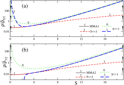
Figure 1: Level density $\rho$ [Eq. (35)], in units of $\overline{\rho}_{\nu}$, with the accurate result “1” (solid line), Eq. (37), $(a)$ for $\nu=5/2$ [MMA1 (i)], and $(b)$, Eq. (39), for $\nu=7/2$ [MMA2 (ii)], shown as functions of the entropy $S$ for different approximations: (1) $S\ll 1$ (dashed lines), Eq. (44) at the second order, and (2) $S\gg 1$ (dotted and rare-dashed lines),  Eq. (43); “0” is the main term of the expansion in powers of $1/S$, and “3” is the expansion over $1/S$ up to first [in $(a)$], and second [in $(b)$] order terms in square brackets of Eq. (43), respectively.

II.3 Shell, isotopic-asymmetry and rotational effects within the MMA

Under the condition of Eq. (31), one can obtain simple analytical expressions for the level density $\rho(E,{\bf Q})$, beyond the standard saddle-point method of both the previous subsection and Appendix B, Eq. (32). Using the integral representation (15) in the adiabatic approximation, one can simplify significantly the square root Jacobian factor $\mathcal{J}^{-1/2}$ [Eq. (19)] by its expansion over small values of $\xi$ or of $1/\xi$; see Eq. (20). Expanding now this Jacobian factor at linear order in $\xi$ and $1/\xi$, one arrives at two different approximations marked below by cases (i) and (ii), respectively. Then, taking the inverse Laplace transformation over $\beta$ in Eq. (15), more accurately (beyond that by the standard saddle-point method), one approximately obtains (see Refs. PRC ; IJMPE ),

$$\rho\approx\rho_{\tt{MMA}}(S)=\overline{\rho}_{\nu}~{}f_{\nu}(S)~{},$$ (35)

$$~{}~{}~{}~{}~{}~{}f_{\nu}(S)=S^{-\nu}I_{\nu}(S)~{},\quad S=2\sqrt{aU}~{}.$$ (36)

Here, $I_{\nu}(S)$ is the modified Bessel function with the index $\nu=\kappa/2+1$ for case (i) and $\nu=\kappa/2+2$ for case (ii), which is determined by the number of the additional integrals of motion above the energy $E$, i.e., the dimension $\kappa$ of the vector ${\bf Q}$. The expression for the entropy $S$ in the argument of this function, $I_{\nu}(S)$, is given by Eq. (II.1) at the saddle point $\boldsymbol{\lambda}=\boldsymbol{\lambda}^{\ast}$. This expression happens to be similar to that of the ideal Fermi gas model, but the level density parameter $a$ in this entropy $S$ is a sum of two semiclassical terms. One of them is the extended Thomas-Fermi term, beyond the Fermi gas approach. Another term is the periodic-orbit shell correction of the Strutinsky’s method BD72 ; see, e.g., Eqs. (17) and (12) in the adiabatic approximation. The excitation energy $U$ is given by Eq. (16) with the explicit dependence on the shell correction $\delta E$ and the rotational frequency $\omega$. For small $\xi\sim\xi^{\ast}\ll 1$, we have case (i), and for large $\xi\sim\xi^{\ast}\gg 1$, we have case (ii), where $\xi^{\ast}$ is, thus, the critical shell-structure quantity, given by expression of Eq. (33).

For the level density $\rho(E,N,Z,M)$ of nuclear spectra, one finds $\nu=5/2$ for case (i) and $7/2$ for case (ii), respectively. In these cases, the modified Bessel function $I_{\nu}(S)$ are expressed in terms of the elementary functions, $\hbox{sinh}(S)$ and $\hbox{cosh}(S)$. In cases (i) and (ii), named below as the MMA1 and MMA2 approaches, respectively, one obtains Eq. (35) with different coefficients $\overline{\rho}_{\nu}$ (see also Refs. PRC ; IJMPE ),

$$\rho_{1}(E,N,Z,M)\cong\rho_{\tt{MMA1}}(S)=\overline{\rho}_{5/2}S^{-5/2}I_{5/2}(S),$$ (37)

$$\overline{\rho}_{5/2}=\frac{(2a)^{5/2}\hbar}{\sqrt{\mathcal{J}_{0}\Theta}}\approx\frac{4\pi^{2}\hbar\sqrt{2}a^{3/2}}{3\Theta^{1/2}}~{},\qquad\mbox{MMA1 (i)},$$ (38)

$$\rho_{2}(E,N,Z,M)\cong\rho_{\tt{MMA2}}(S)=\overline{\rho}_{7/2}S^{-7/2}I_{7/2}(S),$$ (39)

$$\overline{\rho}_{7/2}\approx\frac{(2a)^{7/2}\hbar}{\sqrt{\overline{\xi}\mathcal{J}_{0}\Theta}}\approx\frac{8\pi^{2}\sqrt{2}a^{5/2}}{3\sqrt{\overline{\xi}\Theta}}~{},\qquad\mbox{MMA2 (ii)},~{}$$ (40)

where $\overline{\xi}$ and $\mathcal{J}_{0}$ are given by Eqs. (21) and (22), respectively; see also Eq. (23) for small asymmetry parameter, $X^{2}\ll 1$. Eqs. (37) and (39) depend explicitly on the moment of inertia $\Theta$, which is the sum of the ETF component $\Theta_{\tt{ETF}}$ and shell corrections $\delta\Theta$, $\Theta=\Theta_{\tt{ETF}}+\delta\Theta$. For the Thomas-Fermi approximation to the coefficient $\overline{\rho}_{7/2}$ within the case (ii) one finds NPA ; PRC

$$\rho_{2b}(E,N,Z,M)\cong\rho_{\tt{MMA2b}}(S)=\overline{\rho}^{(2b)}_{7/2}S^{-7/2}I_{7/2}(S),$$ (41)

$$\overline{\rho}^{(2b)}_{7/2}\approx\frac{8\pi\sqrt{3}\lambda a^{5/2}\hbar}{3\sqrt{\Theta}}~{},\qquad\mbox{MMA2b (ii)}.$$ (42)

In the derivation of the coefficient, $\overline{\rho}^{(2b)}_{7/2}$, we assume in Eq. (42) for $\overline{\rho}_{7/2}$ that the magnitude of the relative shell corrections $\mathcal{E}_{\rm sh}$, $\overline{\xi}\propto\mathcal{E}_{\rm sh}$ [see Eqs. (21), (23), and (29)] are extremely small but their derivatives yield large contributions through the level density derivatives $g^{\prime\prime}(\lambda)$, $g\propto A/\lambda$, as in the Thomas-Fermi approach. For large entropy $S$, one finds from Eq. (36)

$$f_{\nu}(S)=\frac{\hbox{exp}(S)}{S^{\nu}\sqrt{2\pi S}}\left[1+\frac{1-4\nu^{2}}{8S}+\mbox{O}\left(\frac{1}{S^{2}}\right)\right].$$ (43)

The same leading results in the expansion (43) for $\nu=5/2$ (i) and $\nu=7/2$ (ii) at large excitation energies $U$ are also derived from the shell-structure Fermi gas formula (32). At small entropy, $S\ll 1$, one also obtains from Eq. (36) the finite combinatorics power expansion St58 ; Er60 ; Ig72 :

$$f_{\nu}(S)=\frac{2^{-\nu}}{\Gamma(\nu+1)}\left[1+\frac{S^{2}}{4(\nu+1)}+\mbox{O}\left(S^{4}\right)\right],$$ (44)

where $\Gamma(x)$ is the gamma function. This expansion over powers of $S^{2}\propto U$ is the same as that of the constant “temperature” model GC65 ; ZK18 ; ZH19 ; KZ20 , used often for the level density calculations, but here, as in Refs. PRC ; IJMPE , we have it without free fitting parameters.

Figure 2: Level density, $\mbox{ln}\rho(E,N,Z)$, for low energy states in nuclei ¹⁴²Nd (a), and ¹⁴⁵Nd (b) were calculated within different approximations: The MMA solid green “1” and black “2a” lines, Eqs.  (66) and (67), at the realistic relative shell correction MSIS12 $\mathcal{E}_{\rm sh}$, respectively; the MMA dashed red line “2b”, Eq. (68), and the Fermi-Gas rare blue dotted line, Eq. (65), approaches are presented. The realistic values of $\mathcal{E}_{\rm sh}$= 0.44 (a), and 0.25 (b) for MMA2 are taken from Ref. MSIS12 (with chemical potentials $\lambda_{n}\approx\lambda_{p}\approx\lambda$, where $\lambda=40$ MeV). Experimental dots with error bars are obtained from the ENSDF database ENSDFdatabase by using the sample method So90 ; IJMPE .

In contrast to the finite MMA limit (44) for the level density, Eq. (35), the asymptotic SFG [Eq. (32)] and FG [Eq. (34)] expressions are obviously divergent at $U\rightarrow 0$. Notice also that the MMA1 approximation for the level density, $\rho(E,N,Z,M)$, Eq. (37), can be applied for large excitation energies, $U$, with respect to the collective rotational excitations. This also the case for the shell-structure Fermi gas (SFG) and Fermi gas (FG) approximations if one can neglect shell effects, $\xi^{\ast}\ll 1$. Thus, the level density $\rho(E,N,Z,M)$ in the case (i), Eq. (37), has a wider range of applicability over the excitation energy variable $U$ than the MMA2 case (ii) [Eq. (39)]. The MMA2 approach has, however, another advantage of describing the important shell structure effects. The main effects of the interparticle interaction, statistically averaged over particle numbers, beyond the shell correction of the mean field, within the Strutinsky’s shell correction method, was taken into account by the extended Thomas-Fermi components of MMA expression (35) for the level density, $\rho(E,N,Z,M)$. These components of $\Omega$ and $a$, Eqs. (3) and (12), respectively, are given by the extended Thomas-Fermi potential, $\Omega_{\rm\tt{ETF}}$, Eq. (II.1), and the level-density parameter, $a_{\rm\tt{ETF}}$, Eq. (13).

In Fig. 1 we show the level density dependence $\rho(S)$, Eq. (35), for $\nu=5/2$ in $(a)$ and $\nu=7/2$ in $(b)$, on the entropy variable $S$ with the corresponding asymptote. In this figure, a small [$S\ll 1$, Eq. (44)] and large [$S\gg 1$, Eq. (43)] entropy $S$ behavior is presented. For small $S\ll 1$ expansion we take into account the quadratic approximation “2”, where $S^{2}\propto U$, that is the same as in the linear expansion within the CTM GC65 ; ZK18 ; ZH19 . For large $S\gg 1$ we neglected the corrections of the inverse power entropy expansion of the pre-exponent factor in square brackets of Eq. (43), lines “0”, and took into account the corrections of the first [$\nu=5/2$, $(a)$] and up to second [$\nu=7/2$, $(b)$] order in $1/S$ (rare dashed lines “3”) to show their slow convergence to the accurate MMA result “1” (35). It is interesting to find almost a constant shift of the results of approximation at large $S$ (dotted line “0”) with the simplest, $\rho\propto\hbox{exp}(S)/S^{\nu+1/2}$, asymptotic saddle point method (SPM) in respect to the accurate MMA results of Eq. (35) (solid line “1”). This may clarify one of the phenomenological models, e.g., the back-shifted Fermi-gas (BSFG) model for the level density DS73 ; So90 ; EB09 .

III Spin-dependences and total level densities

Assuming that there are no external forces acting on a nuclear system, the total angular momentum, ${\bf I}$, and its projection $M$ on a space-fixed axis are conserved, and states with a given energy, $E$, and spin, $I$, are $2I\!+\!1$ degenerate. In this case we use Eq. (37) for $\rho_{1}(E,N,Z,M)$ in the case MMA1 (i) and Eq. (39) for $\rho_{2}(E,N,Z,M)$ [or $\rho_{2b}(E,N,Z,M)$, Eq. (41)] in the case MMA2 (ii) [MMA2b (ii)]. In the first part of this section we will consider the “parallel” rotation, i.e., an alignment of the individual angular momenta of the particle along the axis $0z$ of arbitrary space-fixed coordinate system (see POT shell-structure level density in Refs. KM79 ; PRC ; MK79 ). The second part is devoted to the collective rotation around the axis $0z$, perpendicular to the symmetry axis $0z$ Bj74 ; BM75 ; Ig83 . This section will be ended by the total integrated level-density MMA approach.

III.1 “Parallel” rotations

For the “parallel” rotation around the axis $0z$ of the space-fixed coordinate system (Refs. KM79 ; PRC ; MK79 ), one can use Eqs. (37), (39), and (41) for the level density $\rho(E,N,Z,M)$, where $M$ is the projection of the angular momentum to the axis $0z$. The argument of the Bessel function, $f_{\nu}(S)\propto I_{\nu}(S)$, is the entropy $S(E,N,Z,M)=2\sqrt{aU}$, with the $M$ dependent excitation energy $U$ [Eq. (16)]. Indeed, in the adiabatic mean-field approximation, the POT level density parameter $a$ is given by Eqs. (17) and (13). For the intrinsic excitation energy $U$ [Eq. (16)], one finds

$$U=E-E_{0}-E_{\rm rot}~{},$$ (45)

$$E_{\rm rot}=E^{\parallel}_{\rm rot}(M)=\frac{\hbar^{2}M^{2}}{2\Theta},\quad M=\frac{\Theta}{\hbar}\omega~{},$$ (46)

where, $E_{0}=\tilde{E}+\delta E$, is the same intrinsic (non-rotating) shell-structure energy, as in Eq. (11). With the help of the conservation equations (14) for the saddle point, we deduced the value of the rotation frequency $\omega$, using the second equation in Eq. (46). For the moment of inertia (MI) $\Theta$ with respect to the axis $0z$ in Eq. (45), one has a similar SCM decomposition:

$$\Theta=\tilde{\Theta}+\delta\Theta~{}.$$ (47)

Here, $\tilde{\Theta}$ is the (E)TF MI component which can be approximated by the (E)TF expression, Eq. (A), and $\delta\Theta$ is the MI shell correction for the axially symmetric mean field. This MI can be presented explicitly analytically for the spherically symmetric mean field by Eq. (A10). In Appendix A we present the specific POT derivations by assuming a spherical symmetry of the mean field potential, as full analytical example; see Eq. (A) with Eq. (A10) for the potential shell correction $\delta\Omega(\beta,\lambda,\omega)$ ($\lambda_{n}\approx\lambda_{p}\approx\lambda$).

It is common to use in applications Be36 ; Er60 ; BM67 of the level density its dependence on the spin $I$, $\rho(E,N,Z,I)$. In this subsection, we will consider only the academic axially-symmetric potential case which can be realized practically for the spherical or axial symmetry of a mean nuclear field. Using Eqs. (37), (39), and (41), under the same assumption of a closed rotating system and, therefore, with conservation of the integrals of motion, the spin $I$ and its projection $M$ on the space-fixed axis, one can calculate the corresponding spin-dependent level density $\rho(E,N,Z,I)$ for a given energy $E$, neutron $N$ and proton $Z$ numbers, and total angular momentum $I$ by employing the Bethe formula Be36 ; BM67 ; Ig83 ; So90 ,

$$\rho(E,I) = \rho(E,M=I)-\rho(E,M=I+1)$$ (48)

$$\approx -\left(\frac{\partial\rho(E,M)}{\partial M}\right)_{M=I+1/2}~{}.$$

Here and in the following we omit for simplicity the common arguments $N$ and $Z$. For this level density, $\rho(E,N,Z,I)$, one obtains approximately from Eqs. (37), (39), (41), and (45),

$$\rho(E,I)=\rho_{\rm\tt{MMA}}(E,I)\approx\frac{a\overline{\rho}_{\nu}\hbar^{2}(2I+1)}{\Theta}f_{\nu+1}(S)~{}.$$ (49)

Here, $S$ is the same entropy [$S=2\sqrt{aU}$ from Eq. (36)] given by Eq. (II.1) at the saddle point $\boldsymbol{\lambda}=\boldsymbol{\lambda}^{\ast}$, $a$ is the level density parameter [Eqs. (17) and (12); see also its $\omega^{2}$ correction in Eq. (A12) for the spherical case], $U$ is the excitation energy (45), and $\nu$ equals 5/2 and 7/2, in Eq. (37), and Eqs. (39), and (41), respectively. The multiplier $2I+1$ in Eq. (49) appears because of the substitution $M=I+1/2$ into the derivative in Eq. (48). In order to obtain the approximate MMA total level density $\rho(E,N,Z)$ from the spin-dependent level density $\rho(E,N,Z,I)$, one can multiply Eq. (49) by the spin degeneracy factor $2I+1$ and integrate (sum) over all spins $I$,

$$\rho(E)=\sum_{i}(2I_{i}+1)~{}\rho(E,I_{i})\approx\int dI~{}(2I+1)~{}\rho(E,I)~{}.$$ (50)

Using the expansion of the Bessel functions in Eq. (49) over the argument $S$ for $S\ll 1$ [Eq. (44)], one finds a combinatorics expression. For large $S$ [large excitation energy, $aU\gg 1$, Eq. (43)], one obtains from Eq. (49) the asymptotic Fermi gas expansion. Again, the main term in the expansion for large $S$, Eq. (43), coincides with the full SPM limit to the inverse Laplace integrations in Eq. (II.1). For small angular momentum $I$ and large excitation energy $U_{0}=E-E_{0}$, so that,

$$\frac{E_{\rm rot}(I)}{U_{0}}\approx\frac{\hbar^{2}I(I+1)}{2\Theta~{}U_{0}}\ll 1~{},$$ (51)

one finds the standard separation of the level density, $\rho_{\rm\tt{MMA}}(E,N,Z,I)$, into the product of the dimensionless spin-dependent Gaussian multiplier, $\mathcal{R}(I)$, and another spin-independent factor. Finally, one finds

$$\rho_{\rm\tt{MMA}}(E,I)\approx\frac{\overline{\rho}_{\nu}~{}\mathcal{R}(I)~{}\hbox{exp}\left(S_{0}\right)}{2~{}S_{0}^{\nu-1}\sqrt{2\pi S_{0}}}~{},\quad S_{0}=2\sqrt{aU_{0}}~{},$$ (52)

where $\nu=5/2$ and $7/2$ for cases (i) and (ii), respectively. The Gaussian spin-dependent factor $\mathcal{R}(I)$ is given by

$$\mathcal{R}(I)=\frac{2I+1}{q^{2}}\hbox{exp}\left(-\frac{I(I+1)}{2q^{2}}\right),~{}~{}q^{2}=\frac{\Theta}{\hbar^{2}}\sqrt{\frac{U_{0}}{a}}~{},$$ (53)

where $q^{2}$ is the dimensionless spin dispersion. This dispersion $q^{2}$ at the saddle point, $\beta^{\ast}=1/T=\sqrt{a/U_{0}}$, is the standard spin dispersion $\Theta T/\hbar^{2}$, see Refs. Be36 ; Er60 . Note that the power dependence of the pre-exponent factor of the level density $\rho(E,I)$ on the excitation energy, $U_{0}=E-E_{0}$, differs from that of $\rho(E,M)$; see Eqs. (37), (39), and (52). The exponential dependence, $\rho\propto\hbox{exp}[2\sqrt{a(E-E_{0})}]$, for large excitation energy $E-E_{0}$ is the same for $\nu=5/2$ (i) and $7/2$ (ii), also for any $\nu$ but the pre-exponent factor for the case of $\nu=5/2$ is different than that for the case of $7/2$, see Eq. (52). A small angular momentum $I$ means that the condition of Eq. (51) was applied. Eq. (52) with Eq. (53), are valid for excited states within approximately the condition $1/\tilde{g}\ll U\ll\lambda$, see Eq. (31). For relatively small spins [Eq. (51)] we have the so-called small-spins Fermi-gas model (see, e.g., Refs. Be36 ; Er60 ; GC65 ; BM67 ; Ig83 ; So90 ; KS20 ).

III.2 “Perpendicular” collective rotations

Equations (37), (39), and (41) for the level density $\rho(E,M)$ with the projection $M$ of the angular momentum ${\bf I}$ can be used for the calculations of the level density $\rho(E,N,Z,\mathcal{K})$, where $\mathcal{K}$ is the specific projection of ${\bf I}$ on the symmetry axis of the axially symmetric potential Ig83 ; Bj74 ; BM75 ; MK79 (K in notations of Ref. BM75 , and $\mathcal{K}$ here should not be confused with the inverse level-density parameter). General derivations of these equations applicable for axially symmetric systems in the previous part of this section are specified for a “parallel” rotation and its basic characteristics are presented in Appendix A by using the spherical potential. However, the results for the spin-dependent level density, $\rho(E,I)$ [Eqs. (49)-(52)] cannot be immediately applied for comparison with the available experimental data on rotational bands in the collective rotation of a deformed nucleus. They are studied within the unified rotation model BM75 in terms of the spin $I$ and its projection $\mathcal{K}$ to the internal symmetry axis for deformed axially symmetric nuclei. Following ideas of Refs. Bj74 ; BM75 ; Gr13 ; Gr19 ; Ju98 (see also Refs. Ig83 ; So90 ), we will use another definition of the spin-dependent level density $\rho_{\rm coll}(E,I)$ in terms of the intrinsic level density and collective rotation (and vibration) enhancement. The level density $\rho(E,\mathcal{K})$, e.g., Eqs. (37), (39), and (41) for the level density $\rho(E,M)$ at $M=\mathcal{K}$, is named in Ref. Ig83 as an intrinsic level density,

$$\rho_{\rm int}(U_{\rm coll},\mathcal{K})\equiv\rho(E,M=\mathcal{K}).$$ (54)

In Eqs. (37), (39), (41) and (54), we replace $\Theta$ by the “parallel” moment of inertia $\Theta_{\parallel}$, and $U_{\rm coll}$ by the excitation energy $E-E_{0}-E_{\rm rot}$, where $E_{\rm rot}$ is the collective rotation energy which depends explicitly on the spin projection, $\mathcal{K}$, on the symmetry axis of an axially-symmetric deformed nucleus. Using these expressions, one can define the collective level density as Ig83

$$\rho_{\rm coll}(E,I)=\frac{1}{2}\sum^{I}_{\mathcal{K}=-I}\rho_{\rm int}(U_{0}-E^{\perp}_{\rm rot},\mathcal{K})$$ (55)

$$\approx\frac{1}{2}\int_{-I}^{I}d\mathcal{K}~{}\rho_{\rm int}\left(U_{0}-E^{\perp}_{\rm rot},\mathcal{K}\right)~{},$$ (56)

where $U_{0}=E-E_{0}$ and $E_{\rm rot}=E^{\perp}_{\rm rot}$. The rotation energy $E^{\perp}_{\rm rot}$ for a collective rotation around the axis $0x$ perpendicular to the symmetry axis $0z$ BM75 ,

$$E^{\perp}_{\rm rot}=\left[I(I+1)-\mathcal{K}^{2}\right]/\left(2\Theta_{\perp}\right),$$ (57)

where $\Theta_{\perp}$ is the corresponding (perpendicular to the symmetry axis) moment of inertia, in contrast to the parallel MI $\Theta_{\parallel}$. The factor 1/2 illuminates the reflection degeneracy assuming that the deformation obey the reflection symmetry with respect to the plane, perpendicular to the symmetry axis $0z$. Shell effects in the “perpendicular” moment of inertia, $\Theta_{\perp}$, for any axially symmetric potential well are studied within the periodic orbit theory MA02 ; MY11 ; BB03 ; SM76 in Ref. GM21 .

Substituting Eqs. (37), (39), or (41) with $\Theta=\Theta_{\parallel}$, into Eq. (55), one obtains the MMA expression for the level density, $\rho_{\rm coll}(E,I)$, in terms of the modified Bessel functions. We expand now the expression (55) over the small spin parameters, $E^{\parallel}_{\rm rot}/U_{0}$ and $E^{\perp}_{\rm rot}/U_{0}$. Using the small-spin condition (51), taking approximately $\Theta=\Theta_{\perp}$, and neglecting the effect of $\Theta=\Theta_{\parallel}$ in the exponent, since $\Theta_{\parallel}\ll\Theta_{\perp}$, then one obtains,

$$\rho_{\rm coll}(E,I)=\rho^{\rm coll}_{\rm\tt{MMA}}(E,I)\approx\frac{\overline{\rho}_{\nu}~{}\mathcal{R}_{\rm coll}(I)~{}\hbox{exp}\left(S_{0}\right)}{4~{}S_{0}^{\nu-1}\sqrt{2\pi S_{0}}}~{},$$ (58)

where $S_{0}=2\sqrt{aU_{0}}$, and

$$\mathcal{R}_{\rm coll}(I)=\frac{2I+1}{q^{2}_{\parallel}}\sum_{\mathcal{K}=-I}^{I}\hbox{exp}\left(-\frac{I(I+1)}{2q_{\perp}^{2}}-\frac{K^{2}}{2q^{2}_{\rm eff}}\right)$$

$$\approx\frac{(2I+1)^{2}}{q^{2}_{\parallel}}\hbox{exp}\left(-\frac{(I+1/2)^{2})}{2q_{\perp}^{2}}\right)~{}.$$ (59)

We introduced here several dispersion parameters. Namely, one specifies the effective dispersion parameter, $q^{2}_{\rm eff}$, the parallel, $q^{2}_{\parallel}$, and perpendicular collective parameter, $q^{2}_{\perp}$, which are related to the MI components, $\Theta_{\rm eff}$, $\Theta_{\parallel}$, and $\Theta_{\perp}$, respectively,

$$q_{\rm eff}^{2}=\frac{\Theta_{\rm eff}}{\hbar^{2}}\sqrt{\frac{U_{0}}{a}}~{},~{}~{}~{}\frac{1}{\Theta_{\rm eff}}=\frac{1}{\Theta_{\rm\parallel}}+\frac{1}{\Theta_{\rm\perp}}~{},$$ (60)

$$q_{\rm\parallel}^{2}=\frac{\Theta_{\rm\parallel}}{\hbar^{2}}\sqrt{\frac{U_{0}}{a}},~{}~{}q_{\rm\perp}^{2}=\frac{\Theta_{\rm\perp}}{\hbar^{2}}\sqrt{\frac{U_{0}}{a}}~{}.$$ (61)

The last term in the exponent argument in the first expression of Eq. (III.2) can be neglected for $K^{2}\ll q^{2}_{\rm eff}$. As seen from comparison of Eq. (III.2) with Eq. (53), the collective rotation is much enhanced by the perpendicular dispersion parameter, $q^{2}_{\perp}\gg q^{2}_{\parallel}$, in line of the results obtained in Refs. Bj74 ; BM75 ; Gr13 ; Gr19 ; Ju98 .

A.S. Davydov and his collaborators DF58 ; DC60 have introduced in nuclear physics the possible existence of non-axially symmetric ground-state deformations in some nuclei and applied their model to the description of collective rotations. For non-axial collective rotations, one can obtain the expression for the level density in terms of the internal level density, $\rho_{\rm int}(U_{0}-E^{\rm nax}_{\rm rot})\equiv\rho_{\rm int}(U_{0}-E^{\rm nax}_{\rm rot},0)$, modified with the non-axially rotational energy, $E^{\rm nax}_{\rm rot}$, in terms of the modified Bessel functions. Expanding over small spin parameters, $E^{\rm nax}_{\rm rot}/U_{0}$ [Eq. (51)], one finds Ig83

$$\rho_{\rm coll}(E,I)\approx\frac{1}{2}(2I+1)\rho_{\rm int}\left(U_{0}\right)~{}\hbox{exp}\left[-\frac{(I+1/2)^{2}}{2\overline{q^{2}}}\right]~{},$$ (62)

where $\overline{q^{2}}=(q_{x}^{2}+q_{y}^{2}+q_{z}^{2})/3$ is the averaged value of the spin dispersion parameter, $q_{j}^{2}=\Theta_{j}\sqrt{U_{0}/a}/\hbar^{2}$ are partial dispersions, $j=x,y$, and $z$. In these derivations, we neglected partial $\mathcal{K}^{2}$ components with respect to $\overline{q^{2}}$, and $I(I+1)\approx(I+1/2)^{2}$ in the semiclassical approximation.

III.3 Total integrated MMA level densities

For a comparison with experimental data ENSDFdatabase , we present also the level density $\rho(E,N,Z)$ obtained by the integration of $\rho(E,N,Z,M)$ over the angular momentum projection $M$. The statistics conditions have improved PRC ; IJMPE , so that we can study a longer chain of isotopes, including those relatively far away from the beta stability line. Including the shell and isotopic asymmetry effects, for the standard saddle-point method approach [Eq. (32)] one arrives at (see Ref. IJMPE )

$$\rho(E,N,Z)=\sum_{M}\rho(E,N,Z,M)\approx\int dM\rho(E,N,Z,M)$$ (63)

$$\approx\frac{a^{3/4}\hbox{exp}(2\sqrt{aU_{0}})}{4\pi~{}U^{5/4}~{}\sqrt{\pi\mathcal{J}_{0}(1+\xi^{\ast})}}\approx\frac{\sqrt{\pi}\hbox{exp}(2\sqrt{aU_{0}})}{12a^{1/4}~{}U^{5/4}~{}\sqrt{1+\xi^{\ast}}}~{}.$$ (64)

Here, the summation and approximate integration are carried out over all spin projections $M$. In Eq. (64), $a=\pi^{2}g(\lambda)/6$ is the total level density parameter, Eqs. (17) and (13); $\mathcal{J}_{0}$ is the component of the Jacobian $\mathcal{J}$, Eq. (22), which is independent of $\beta$ but depends on the shell structure; $U_{0}$ is the excitation energy $U$ [Eq. (45)] at zero angular momentum projection, $M=0$; see also Eq. (33) for $\xi^{\ast}$. The asterisk means $\beta=\beta^{\ast}=\sqrt{a/U}$ at the saddle point. In the second equation of (32), and of (33) we also used $\lambda_{n}\approx\lambda_{p}\approx\lambda$ for a small asymmetry parameter, $X^{2}$, together with Eq. (A15) for the derivatives of the energy shell corrections and Eq. (A14) for the mean distance between neighboring major shells near the Fermi surface, $\mathcal{D}\approx\lambda/A^{1/3}$.

As in section II.2, at large excitation energy, Eq. (64) is a more general shell-structure Fermi-gas (SFG) asymptotic with respect to the well-known Be36 ; Er60 ; GC65 Fermi gas (FG) approximation for $\rho(E,N,Z)$, which is equal to Eq. (64) at $\xi^{\ast}\rightarrow 0$,

$$\rho(E,N,Z)\rightarrow\frac{\sqrt{\pi}\hbox{exp}(2\sqrt{aU})}{12a^{1/4}~{}U^{5/4}}~{}.$$ (65)

Similarly, as in section II.3, according to the general definitions in Eq. (63), for the total integrated MMA level density, one has Eq. (35) (Ref. IJMPE ) but with the entropy $S$ given by $S=2\sqrt{aU_{0}}$ [Eq. (45) for the excitation energy $U$ but at $M=0$]. In cases (i) and (ii), named below the MMA1 and MMA2 approaches, respectively, one obtains Eq. (35) with different coefficients $\overline{\rho}_{\nu}$ (see also Refs. PRC ; IJMPE ),

$$\rho_{\tt{MMA1}}(S)=\overline{\rho}_{2}S^{-2}I_{2}(S),\qquad\overline{\rho}_{2}=\frac{2a^{2}}{\pi\sqrt{\mathcal{J}_{0}}}\approx\frac{2\pi a}{3}\qquad\mbox{(i)},$$ (66)

$$\rho_{\tt{MMA2}}(S)=\overline{\rho}_{3}S^{-3}I_{3}(S),\qquad\overline{\rho}_{3}\approx\frac{4a^{3}}{\pi\sqrt{\overline{\xi}\mathcal{J}_{0}}}\approx\frac{4\pi a^{2}}{3\sqrt{\overline{\xi}}}\qquad\mbox{(ii)},~{}$$ (67)

with the same $\overline{\xi}$ and $\mathcal{J}_{0}$ given by Eqs. (21) and (22), respectively; see also Eq. (23). For the TF approximation to the coefficient $\overline{\rho}_{3}$ within the case (ii), one finds NPA ; PRC ; IJMPE

$$\rho_{\tt{MMA2b}}(S)=\overline{\rho}^{(2b)}_{3}S^{-3}I_{3}(S),\qquad\overline{\rho}^{(2b)}_{3}\approx\frac{2\sqrt{6}~{}\lambda a^{2}}{3}~{}.$$ (68)

IV Discussion of the results

Fig. 2 and Table I show results of different theoretical approaches [MMA, Eqs. (66), (67), and (68); SFG, Eq. (64), and; standard FG, Eq. (65)] for the statistical level density $\rho(E,N,Z)$ (in logarithms) as functions of the excitation energy $U$. They are compared to the experimental data obtained by the sample method So90 ; PRC ; IJMPE . In Fig. 2 and Table I, we present the results of the total MMA level density, $\rho(E,N,Z)$, [Eqs. (66) for the MMA1, (67) for the MMA2 and (68) for the MMA2b approaches] for the inverse level-density parameter $K$ obtained from a least mean-square fit of the calculated level density to the experimental data ENSDFdatabase that was deduced by using the sample method PRC ; IJMPE ; NPA . The control relative error-dispersion parameter $\sigma$ is determined in terms of $\chi^{2}$ of the least mean-square fit by the standard formulas:

$$\sigma^{2}=\frac{\chi^{2}}{\aleph-1},\qquad\chi^{2}=\sum_{i}\frac{(y(U_{i})-y^{\rm exp}_{i})^{2}}{(\Delta y_{i})^{2}},\qquad y=\ln\rho~{},$$ (69)

where $\aleph$ is the sample number and $\Delta y_{i}\sim 1/\sqrt{N_{i}}$ and $N_{i}$ is a number of level states in the sample, $i=1,2,3\ldots,\aleph$.

Table 1: The inverse level-density parameter $K$ (with errors $\Delta K$ in parenthesis) in units of MeV, found by the least mean-square fit for ^131-156Nd in the low energy states ranges restricted by maximal values of the excitation energy having clear spins (from the ENSDF database ENSDFdatabase ), and $U_{\rm max}$ (also in MeV units), with the precision of the standard expression for $\sigma$, Eq. (69), are shown for several approximations with the same notations as in Fig. 2; asterisks mean results of calculations, accounting for pairing with $E_{\rm cond}=0.72$ MeV for $A=140$ and $0.69$ MeV for $A=142$; see also text. The MMA approaches are presented with minimal $\sigma$ which were obtained for the corresponding one-component systems of $A$ nucleons PRC .

		FG		SFG		MMA1		MMA2a		MMA2b		One-component system
	$U_{\rm max}$ MeV	$K$($\Delta K$) MeV		$K$($\Delta K$) MeV		$K$($\Delta K$) MeV		$K$($\Delta K$) MeV		$K$($\Delta K$) MeV			$K$($\Delta K$) MeV
$A$			$\sigma$		$\sigma$		$\sigma$		$\sigma$		$\sigma$	Approach		$\sigma$
131	1.57	7.56 (1.2)	10.8	7.47 (1.1)	19.7	7.01 (1.1)	12.3	8.49 (0.92)	9.1	18.8 (1.4)	4.5	MMA2b	26.2 (1.6)	3.7
132	3.66	18.7 (1.0)	4.4	18.3 (0.9)	4.3	17.7 (1.1)	5.4	19.4 (0.7)	3.5	34.9 (0.3)	0.7	MMA2b	47.2 (0.6)	0.8
133	0.55	3.8 (0.2)	2.2	3.8 (0.2)	2.2	3.5 (0.2)	2.7	7.3 (0.2)	1.0	13.2 (0.5)	1.1	MMA2b	19.0 (0.8)	1.3
134	1.42	10.7 (0.7)	1.7	10.2 (0.6)	1.7	9.89 (0.7)	2.1	11.3 (0.5)	1.6	26.0 (1.5)	1.3	MMA2b	39.1 (3.8)	2.2
135	0.56	4.5 (0.6)	3.2	4.5 (0.6)	3.2	4.1 (0.6)	3.6	10.0 (0.8)	2.0	15.8 (1.3)	1.7	MMA2b	23.6 (2.4)	2.0
136	1.75	16.6 (1.1)	1.4	15.2 (0.9)	1.3	14.9 (1.2)	1.8	25.6 (0.9)	0.8	39.4 (1.1)	0.5	MMA2b	56.4 (1.6)	0.5
137	2.47	13.7 (1.1)	5.7	13.7 (1.1)	5.7	12.8 (1.1)	6.9	21.8 (0.8)	2.7	28.4 (0.8)	2.0	MMA2b	38.9 (1.1)	1.8
138	2.32	15.9 (0.7)	1.9	15.8 (0.7)	1.9	15.0 (0.5)	1.7	19.0 (0.9)	2.3	32.8 (2.6)	3.2	MMA2a	23.0 (1.2)	2.5
139	0.93	7.3 (0.9)	3.3	7.2 (0.9)	3.3	6.7 (0.9)	3.8	9.5 (0.8)	2.7	21.0 (1.8)	2.0	MMA2b	32.7 (3.6)	2.3
140	3.49	19.1 (0.5)	2.3	18.3 (0.5)	2.2	18.2 (0.5)	2.3	18.7 (0.4)	2.3	35.0 (1.5)	3.2	MMA2a	22.4 (0.6)	2.3
												MMA2b*	30.3 (1.4)	2.7
141	1.62	12.7 (0.9)	2.1	12.0 (0.8)	2.1	11.8 (0.9)	2.3	13.0 (0.7)	2.0	29.3 (1.8)	1.7	MMA2b	42.6 (4.0)	2.3
142	3.42	19.8 (0.4)	1.3	17.7 (0.3)	1.4	18.9 (0.3)	1.1	16.9 (0.2)	1.2	36.1 (1.4)	2.6	MMA2a	20.5 (0.3)	1.4
												MMA2b*	31.5 (1.3)	2.2
143	1.91	13.5 (0.7)	2.1	12.6 (0.6)	2.1	12.7 (0.7)	2.2	13.1 (0.6)	2.0	29.4 (1.3)	1.5	MMA2b	43.2 (2.4)	1.8
144	2.30	17.0 (0.7)	1.7	16.0 (0.7)	1.7	16.0 (0.7)	1.7	15.8 (0.6)	1.7	35.3 (2.3)	2.3	MMA2a	19.2 (1.0)	2.3
145	1.72	10.5 (0.5)	2.9	10.3 (0.4)	2.9	9.9 (0.6)	4.1	11.1 (0.4)	2.7	24.0 (0.7)	1.7	MMA2b	33.1 (1.2)	2.0
146	1.81	14.0 (0.7)	1.7	13.6 (0.6)	1.8	13.2 (0.6)	1.8	14.1 (0.6)	1.8	31.3 (2.4)	2.5	MMA2a	17.0 (0.7)	1.8
147	1.21	8.3 (1.0)	5.6	9.1 (0.8)	4.9	7.6 (1.0)	6.9	8.2 (0.9)	5.6	21.7 (1.3)	2.5	MMA2b	3.6 (1.8)	2.2
148	1.78	12.1 (0.5)	2.1	15.5 (0.8)	2.6	11.4 (0.4)	2.2	12.2 (0.4)	2.2	26.9 (1.9)	2.3	MMA2a	14.7 (0.6)	2.3
149	0.81	5.1 (0.7)	6.6	5.1 (0.7)	6.5	4.7 (0.5)	4.9	6.3 (0.6)	5.3	16.5 (1.1)	2.7	MMA2b	23.6 (1.4)	2.3
150	1.20	9.5 (0.6)	2.1	9.3 (0.5)	2.1	8.9 (0.6)	2.6	9.8 (0.5)	2.1	24.6 (1.9)	2.4	MMA2a	12.1 (0.4)	1.4
151	1.93	3.9 (0.8)	7.2	3.5 (0.7)	8.5	3.5 (0.7)	8.5	4.8 (0.6)	5.9	14.5 (1.4)	3.1	MMA2b	21.0 (1.9)	2.8
152	1.90	12.4 (0.7)	3.4	11.8 (0.6)	3.3	11.7 (0.8)	4.3	11.7 (0.5)	3.5	27.6 (1.7)	3.4	MMA2a	14.0 (0.6)	3.3
153	1.58	9.2 (1.3)	9.6	8.9 (1.2)	9.5	8.5 (1.3)	11.3	9.1 (1.0)	9.0	22.7 (1.4)	3.7	MMA2b	31.7 (1.7)	3.0
154	1.35	10.9 (0.8)	2.6	10.5 (0.7)	2.5	10.1 (0.9)	3.4	10.6 (0.6)	2.6	27.8 (1.5)	1.8	MMA2a	13.0 (0.8)	2.7
155	1.83	13.7 (2.4)	6.0	12.9 (2.1)	5.9	12.2 (2.4)	7.7	12.1 (1.7)	6.4	32.2 (2.5)	2.6	MMA2b	47.8 (5.3)	3.5
156	2.74	17.6 (1.5)	6.0	16.1 (1.2)	5.8	16.5 (1.6)	7.2	15.4 (1.1)	6.4	35,7 (1.6)	2.9	MMA2b	48.9 (2.2)	2.7

We determine $\sigma$, Eq. (69), at the minimum of $\chi^{2}$ over the unique parameter, $K=K_{\rm min}$, having a definite physical meaning as the inverse level-density parameter $K$ (see Figs. 2 and 3). Then, we may compare the values of $\sigma$ for several different MMA approximations to the level density approaches (Fig. 3), which were found independently of the data, under certain statistical conditions mentioned above. For this aim we are interested in the lowest value obtained for $\sigma(K_{\rm min})$ by fitting calculated results of different theoretical approaches. The MMA results for the minimal values of $\sigma$, Eq. (69), are shown in plots of Fig. 4 by black solid lines as the best, among the MMA approaches, agree with the experimental data. The results of our calculations are almost independent of the sample number, $\aleph=5-7$, which plays the same role as an averaging parameter on the plateau condition in the Strutinsky averaging procedure BD72 .

As done in Refs. PRC ; IJMPE for several isotopes, Fig. 2 and Table I present the two opposite situations concerning the states distributions as functions of the excitation energy $U=U_{0}=E-E_{0}$ [Eq. (45) at $M=0$]. We show results for the nucleus ¹⁴⁵Nd (b) with a large number of the low energy states below excitation energy of about 1 MeV. For ¹⁴²Nd (a) one has a very small number of low energy states below the same energy of about 1 MeV (see ENSDF database ENSDFdatabase and Table I for maximal excitation energies $U_{\rm max}$). But there are many states in ¹⁴²Nd with excited energies of above 1 MeV up to essentially larger excitation energy of about 2-4 MeV. According to Ref. MSIS12 , the shell effects, measured by $\mathcal{E}_{\rm sh}$, Eq. (29), are significant in both these nuclei, a slightly deformed ¹⁴⁵Nd and spherical ¹⁴²Nd, see Fig. 3(b).

In Fig. 2 and Table I, the results of the MMA1 and MMA2 approaches, Eqs. (66) and (67), respectively, are compared with the FG approach, Eq. (65). The SFG results, Eq. (64), are very close to those of the well-known FG asymptote, Eq. (65), which neglects the shell effects; see Table I. Therefore, they are not shown in Fig. 2. The results of the MMA2a approach, Eq. (67), in the dominating shell effects case (ii) [$\xi^{\ast}\gg 1$, Eq. (33)] with the realistic relative shell correction, $~{}\mathcal{E}_{\rm sh}~{}$ (Ref. MSIS12 ), are shown versus those of a small shell effects approach MMA1 (i), Eq. (66), valid at $~{}\xi^{\ast}\ll 1~{}$. The results of the limit of the MMA2 approach to a very small value of $~{}\mathcal{E}_{\rm sh}$, but still within the case (ii), Eq. (68), named as MMA2b, are also shown in Fig. 2 and Table I because of a large shell structure contribution due to relatively large derivatives of the energy shell corrections over the chemical potential. They are in contrast to the results of the MMA1 approach. The results of the SFG asymptotical full saddle-point approach, Eq. (64), and of a similar popular FG approximation, Eq. (65), are both in good agreement with those of the standard Bethe formula Be36 for one-component systems (see Ref. PRC ), and are also presented in Table I. For finite realistic values of $\mathcal{E}_{\rm sh}$, the value of the inverse level-density parameter $K$ of the MMA2a (Table I) and the corresponding level density (Fig. 2) are in between those of the MMA1 and MMA2b. Sometimes, the results of the MMA2a approach are significantly closer to those of the MMA1 one, than to those of the MMA2b approach, e.g., for nuclei as ¹⁴²Nd.

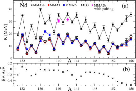
Figure 3: Inverse level-density parameters $K$ (with errors) for available Nd isotopes are shown as function of the particle numbers $A$ within a long chain $A=131-156$ [panel (a)]. Different symbols correspond to several approximations: the close black dots for the MMA2b [Eq. (68)], full red squares for MMA1 [Eq. (66)], larger blue open squares for MMA2a [Eq. (67)], and big open circles for Fermi gas (FG) [Eq. (65)] approaches. “MMA2b with pairing” points account for the excitation energy shift due to pairing condensation Ig83 ; So90 ; PRC ; SC19 with the best (smallest) $\sigma$ compared with other approaches. In panel (b), the relative energy shell corrections, $\delta E$, are shown in units of the averaged energy per particle number $A$ MSIS12 .

In both panels of Fig. 2, one can see the divergence of the FG approach [Eq. (65)], as well as of the SFG approach [Eq. (64)], in the full SPM level-density asymptote in the zero-excitation energy limit $U\rightarrow 0$. This is clearly seen also analytically, in particular in the FG limit, Eq. (65); see also the general asymptotic expression (43). It is, obviously, in contrast to any MMAs combinatorics expressions (44) in this limit; see Eqs. (66)-(68). The MMA1 results are close to those of the FG and SFG approaches for all considered nuclei (Table I), in particular, for both ¹⁴²Nd and ¹⁴⁵Nd isotopes in Table I. The reason is that their differences are essential only for extremely small excitation energies $U$, where the MMA1 approach is finite while other, FG and SFG, approaches are divergent. However, there are almost no experimental data for excited states in the range of their differences, at least in the nuclei under consideration.

The MMA2(b) results, Eq. (68), for ¹⁴⁵Nd [see Fig. 2(b)] with $\sigma\sim 1$ are significantly better in agreement with the experimental data as compared to the results of all other approaches (for the same nucleus). For this nucleus, the MMA1 [Eq. (66)], FG [Eq. (65)], and SFG [Eq. (64)] approximations are characterized by much larger $\sigma$ (see Table I). In contrast to the case of ¹⁴⁵Nd [Fig. 2(b)] with excitation energy spectrum having a large number of low energy states below about 1 MeV, for ¹⁴²Nd [Fig. 2(a)] with almost no such states in the same energy range, one finds the opposite case –  a significantly larger MMA2b value of $\sigma$ as compared to those for other approximations (Fig. 2 and Table I). In particular, for MMA1 [case (i)], and other asymptotic approaches FG and SFG, one obtains for ¹⁴²Nd spectrum almost the same $\sigma\sim 1$, and almost the same for MMA2a [case (ii)] with realistic values of $\mathcal{E}_{\rm sh}$. Again, notice that the MMA2a results [Eq. (67)] are closer, at the realistic $\mathcal{E}_{\rm sh}$, to those of the MMA1 [case (i)], as well as the results of the FG and SFG approaches. The MMA1 and MMA2a results (at realistic values of $\mathcal{E}_{\rm sh}$) as well as those of the FG and SFG approaches are obviously better in agreement with the experimental data ENSDFdatabase (see Refs. PRC ; IJMPE ) for ¹⁴²Nd [Fig. 2(a)].

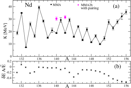
Figure 4: (a) Inverse level-density parameter $K$ (with errors) for Nd isotopes is shown as function of the particle number $A$ within a long chain A=131-156: the close black dotted points are for the MMA approach taken with the smallest relative error parameter $\sigma$, Eq. (69), among all MMAs. (b): The relative shell correction energies, $\delta EA/\tilde{E}$, are taken from Ref. MSIS12 .

One of the reason for the exclusive properties of ¹⁴⁵Nd [Fig. 2(b)], as compared to ¹⁴²Nd [Fig. 2(a)], might be assumed to be the nature of the excitation energy in these nuclei. Our MMAs results [case (i)] or [case (ii)] could clarify the excitation nature as assumed in Refs. PRC ; IJMPE . Since the MMA2b results [case (ii)] are much better in agreement with the experimental data than the MMA1 results [case (i)] for ¹⁴⁵Nd, one could presumably conclude that for ¹⁴⁵Nd one finds more clear thermal low-energy excitations. In contrast to this, for ¹⁴²Nd [Fig. 2(a)], one observes more regular high-energy excitations due to, e.g., the dominating rotational excitations, see Refs. KM79 ; PRC ; IJMPE . As seen, in particular, from the values of the inverse level-density parameter $K$ and the shell structure of the critical quantity, Eq. (33), these properties can be understood to be mainly due to the larger values of $K$ and shell correction second derivative $\mathcal{E}^{\prime\prime}_{\rm sh}$, for low energy states in ¹⁴⁵Nd (Table I) versus those of the ¹⁴²Nd spectrum. This is in addition to the shell effects, which are very important for the case (ii) which is not even realized without their dominance.

As results, the statistically averaged level densities $\rho(E,N,Z)$ for the MMA approach with a minimal value of the control-error parameter $\sigma$, Eq. (69), in plots of Fig. 2 agree well with those of the experimental data. The results of the MMA, SFG and FG approaches for the level densities $\rho(E,N,Z)$ in Fig. 2, and for $K$ in Table I, do not depend on the cut-off spin factor and moment of inertia because of the summations (integrations) over all spins projections, or over spins, indeed, with accounting for the degeneracy $2I+1$ factor. We do not use empiric free fitting parameters in our calculations, in particular, for the FG results shown in Table I, in contrast to the back-shifted Fermi gas DS73 and constant temperature models, see also Ref. EB09 .

The results of calculations for the inverse level-density parameter $K$ in the long Nd isotope chain with $A=131-156$ are summarized in Fig. 3 and Table I. Preliminary spectra data for nuclei far away from the $\beta$-stability line from Ref. ENSDFdatabase are included in comparison with the results of the theoretical approximations. These experimental data may be incomplete. Nevertheless, it might be helpful to present a comparison between theory and experiment to check general common effects of the isotopic asymmetry and shell structure in a wide range of nuclei around the $\beta$-stability line.

As seen in Fig. 3, the results for $K$ for the isotopes of Nd ($Z=60$) as a function of the particle number $A$ are characterized by a very pronounced saw-toothed behavior with alternating low and high $K$ values for odd and even nuclei, respectively. As for the platinum chain in Ref. IJMPE , this behavior is more pronounced for the MMA2b (close black dots) approach with larger $K$ values. For each nucleus, the significantly smaller MMA1 value of $K$ (full red squares) is close to that of the FG approach (heavy open black circles). The SFG results are very close to those of the FG approach and, therefore, are not shown in the plots, but presented in Table I. The MMA2a results for $K$ are intermediate between the MMA2b and MMA1 ones, but closer to the MMA1 values.

Notice that for the rather long chain of isotopes of Nd, as for Pt ones IJMPE , one finds a remarkable shell oscillation (Fig. 3). Fixing the even-even (even-odd) chain, for all compared approximations, one can see a hint of slow oscillations by evaluating its period $\Delta A$, $\Delta A\sim 30$ for $A\sim 140$ (see Refs. NPA ; IJMPE ). Within order of magnitude, these estimates agree with the main period for the relative shell corrections, $\delta EA/\tilde{E}$, shown in Fig. 3(b). Therefore, according to these evaluations and Fig. 3(b) for $K(A)$, we show the sub-shell effects within a major shell. This shell oscillation as function of $A$ is more pronounced for the MMA2b case because of its relatively large amplitude, but is mainly proportional to that of the MMA2a and other approximations.

The MMAs results shown in Fig. 3, as function of the particle number $A$, Eq. (64), can be partially understood through the basic critical quantity, $\xi\sim\xi^{\ast}\leq\xi^{\ast}_{\rm max}$, where $\xi^{\ast}_{\rm max}\propto KU_{\rm max}\mathcal{E}^{\prime\prime}_{\rm sh}/A^{4/3}$. Here we need also the maximal excitation energies $U_{\rm max}$ of the low energy states (from Ref. ENSDFdatabase and Table I) used in our calculations. Such low energy states spectra are more complete due to information on the spins of the states. As assumed in the derivations (Subsection II.3), larger values of $\xi^{\ast}$, Eq. (33), are expected in the MMA2b approximation (see Fig. 3), due to large values of $K$ (small level density parameter $a$). For the MMA1 approach, one finds significantly smaller $\xi^{\ast}$, and in between values (closer to those of the MMA1) for the MMA2a case. This is in line with the assumptions for case (i) and case (ii) in the derivations of the level-density approximations of the MMA1, Eq. (37), and MMA2, Eq. (39), respectively.

In order to clarify the shell effects, we present in Fig. 4(a) the inverse level-density parameters $K(A)$ taking the MMA results with the smallest values of $\sigma$ for each nucleus (see also Fig. 3 and Table I). Among all MMAs results, this provides the best agreement with the experimental data for the statistical level density obtained by the sample method PRC ; IJMPE . The relative energy-shell corrections MSIS12 , $\delta EA/\tilde{E}$, are presented too by crosses in Figure 4(b).

The oscillations in Fig. 4(a) are associated with sub-shell effects within the major shell, shown in Fig. 4(b). As seen from Fig. 4 and Table I, the results of the MMA2b approach better agree with experimental data the larger number of states in the low energy states range and the smaller maximal excitation energies, $U_{\rm max}$. This is not the case for the MMA1 and other approaches. One of the most pronounced cases was considered above for the ¹⁴⁵Nd and ¹⁴²Nd nuclei. However, sometimes, e.g., for ^148,150Nd, the results of all approximations are not well distinguished because of almost the same $\sigma$. Except for such nuclei, for significantly smaller $U_{\rm max}$ the results of the MMA2b approach are obviously better than the results of other approaches. Most of the Nd isotopes under consideration are well deformed, and the excited energy spectra (Ref. ENSDFdatabase ) begin with relatively small energy levels in the low energy states region, except for ^140,142Nd with relatively large $U_{\rm max}$ (see Table I). Therefore, the pairing effects Ig83 ; So90 ; SC19 were taken into account in these two nuclei in our Nd calculations in the simplest version PRC of a shift of the excitation energy by pairing condensation energy (see the results which follow the asterisks in Table I). Pairing correlations decrease somehow the inverse level-density parameter $K$ and smooth the sawtooth-like behavior of $K(A)$ as function of the particle number $A$ (Fig. 3). Accounting for pairing effects, one can observe improvement of the results for the same MMA2b approach. We should emphasize once more that the MMA2 approach for each nucleus is important in the case (ii) of dominating shell effects (see Subsection II.3). As shown in Table I, the isotopic asymmetry effects are more important than those of the corresponding one-component nucleon case PRC . They change significantly the inverse level-density parameter $K$, especially for the MMA2b approach.

Thus, for the Nd isotope chain, one can see almost one major shell for mean values of $K(A)$ for each approximation (Fig. 3). The MMA1 (or SFG and FG) approach yields essentially small values for $K$, which are closer to that of the neutron resonances. Their values differ a little from those of the MMA2a approach for smaller particle numbers, almost the same for larger particle numbers, and much smaller than those of the MMA2b approach (Fig. 3). As seen clearly from Figs. 3 and 4, and Table I, in line with results of Refs. ZS16 ; ZH19 , the obtained values for $K$ within the MMA2 approach can be essentially different from those of the MMA1 approach and those of the SFG and FG approaches found, mainly, for the neutron resonances. Notice that, as in Refs. NPA ; PRC ; IJMPE , in all our calculations of the statistical level density, $\rho(E,N,Z)$, we did not use a popular assumption of small spins at large excitation energies $U$, which is valid for the neutron resonances. Largely speaking, for the MMA1 approach, one finds values for $K$ of the same order as those of the FG and SFG approaches. These mean values of $K$ are mostly close to those of neutron resonances in order of magnitude. The results for $K$ of the FG and SFG approaches, Eqs. (65) and (64), respectively, can be understood because neutron resonances appear relatively at large excitation energies $U$. For these resonances, for the MMA1 approach we should not expect such strong shell effects as assumed to be in the MMA2b approach. More systematic study of large deformations, neutron-proton asymmetry, and pairing correlations (see Refs. Er60 ; Ig83 ; So90 ; AB00 ; AB03 ; ZH19 ; KZ20 ) should be taken into account to improve the comparison with experimental data, see also preliminary estimates in Ref. PRC for the rare earth and the double magic spherical nucleus ²⁰⁸Pb.

V Conclusions

We have derived the statistical level density $\rho(S)$ as function of the entropy $S$ within the micro-macroscopic approximation (MMA) using the mixed micro- and grand-canonical ensembles, accounting for the neutron-proton asymmetry and collective rotations of nuclei beyond the saddle point method of the standard Fermi gas (FG) model. This function can be applied for small and, relatively, large entropies $S$, or excitation energies $U$ of a nucleus. For a large entropy (excitation energy), one obtains the exponential asymptote of the standard saddle-point Fermi-gas model, however, with significant inverse, $1/S$, power corrections. For small $S$ one finds the usual finite combinatorics expansion in powers of $S^{2}$. Functionally, the MMA linear approximation in the $S^{2}\propto U$ expansion, at small excitation energies $U$, coincides with that of the empiric constant “temperature” model, obtained, however, without using free fitting parameters. Thus, the MMA reproduces the well-known Fermi-gas approximation (for large entropy $S$) with the constant “temperature” model for small entropy $S$, also with accounting for the neutron-proton asymmetry and rotational motion. The MMA at low excitation energies clearly manifests an advantage over the standard full saddle-point approaches because of no divergences of the MMA in the limit of small excitation energies, in contrast to all of full saddle-point method, e.g., the Fermi gas asymptote. Another advantage takes place for nuclei which have a lot of states in the very low-energy states range. In this case, the MMA results with only one physical parameter in the least mean-square fit, the inverse level-density parameter $K$, is usually the better the larger number of the extremely low energy states. These results are certainly much better than those for the Fermi gas model. The values of the inverse level-density parameter $K$ are compared with those of experimental data for low energy states below neutron resonances in nuclear spectra of several nuclei. The MMA values of $K$ for low energy states can be significantly different from those of the neutron resonances, studied successfully earlier within the Fermi gas model.

We have found a significant shell effects in the MMA level density for the nuclear low-energy states range within the semiclassical periodic-orbit theory. In particular, we generalized the known saddle-point method results for the level density in terms of the full shell-structure Fermi gas (SFG) approximation, accounting for the shell, the neutron-proton asymmetry, and rotational effects, using the periodic-orbit theory. Therefore, a reasonable description of the experimental data for the statistically averaged level density, obtained by the sample method for low energy states was achieved within the MMA with the help of the semiclassical periodic-orbit theory. We emphasize the importance of the shell, neutron-proton asymmetry, and rotational effects in these calculations. We obtained values of the inverse level-density parameter $K$ for low-energy states range which are essentially different from those of neutron resonances. Taking a long Nd isotope chain as a typical example, one finds a saw-toothed behavior of $K(A)$ as function of the particle number $A$ and its remarkable shell oscillation. We obtained values of $K$ that are significantly larger than those obtained for neutron resonances, due mainly to accounting for the shell effects. We show that the semiclassical periodic-orbit theory is helpful in the low-energy states range for obtaining analytical descriptions of the level density and energy shell corrections. They are taken into account in the linear approximation up to small corrections due to the residual interaction beyond the mean field and extended Thomas-Fermi approximation within the shell-correction method, see Refs. BD72 ; BK72 . The main part of the inter-particle interaction is described in terms of the extended Thomas-Fermi counterparts of the statistically averaged nuclear potential, and in particular, of the level density parameter.

Our MMA approach for accounting for the spin dependence of the level density was extended to the collective rotations of deformed nuclei within the unified rotation model. The well-known effects of the enhancement due to the nuclear collective rotations were considered with accounting for the shell structure and neutron-proton asymmetry. This approach might be interesting in the study of the isomeric states in the strong deformed nuclei at high spins due to the shell effects RB80 ; St87 . We suggest also to work out the MMA approach for the description of the collective rotations of nuclei, accounting for the phase transitions from the axial to non-axial deformations MM10 ; MM12 .

Our approach can be applied to the statistical analysis of the experimental data on collective nuclear states, in particular, for the nearest-neighbor spacing distribution calculations within the Wigner-Dyson theory of quantum chaos Ze96 ; Ze16 ; GK11 . As the semiclassical periodic-orbit MMA is the better the larger particle number in a Fermi system, one can apply this method also for study of the metallic clusters and quantum dots in terms of the statistical level density, and of several problems in nuclear astrophysics. As perspectives, the collective rotational excitations at large nuclear angular momenta and deformations, as well as more consequently pairing correlations, all with a more systematic accounting for the neutron-proton asymmetry, will be taken into account in a future work. In this way, we expect to improve the comparison of the theoretical evaluations with experimental data on the level density parameter significantly for energy levels below the neutron resonances.

Appendix A Semiclassical periodic-orbit theory for isotopically asymmetric rotating system

Introducing the isotopic index $\tau=\{n,p\}$ for isotopically asymmetric nuclear system, one can present the partition function $\ln\mathcal{Z}$ as sum of $\ln\mathcal{Z}_{\tau}$, $\ln\mathcal{Z}=\ln\mathcal{Z}_{n}+\ln\mathcal{Z}_{p}$. In the case of the “parallel” rotation (alignment of the angular momenta of individual particles along the symmetry axis $0z$), one has for a spherical and axial symmetric potential the explicit $\tau$ partition-function component:

$$\ln\mathcal{Z}_{\tau}=\sum\limits_{i}\ln\left\{1+\hbox{exp}\left[\beta\left(\lambda_{\tau}-\varepsilon_{i}+\hbar\omega m_{i}\right)\right]\right\}$$

$$\approx\int\limits_{0}^{\infty}\hbox{d}\varepsilon\int\limits_{-\infty}^{\infty}\mbox{d}m~{}g_{\tau}(\varepsilon,m)\ln\left\{1+\right.$$

$$+\left.\hbox{exp}\left[\beta\left(\lambda-\varepsilon+\hbar\omega m\right)\right]\right\}~{}.$$ (A1)

Here, $\varepsilon_{i}$ and $m_{i}$ are the single-particle (s.p.) energies and projections of the angular momentum on the symmetry axis $Oz$ of the quantum states $i$ of the $\tau$ system in the axially symmetric mean-field potential well, respectively. In the transformation from the sum to an integral, we introduced the s.p. level density $g_{\tau}(\varepsilon,m)$ as a sum of the smooth, $\tilde{g}_{\tau}$, and oscillating shell, $\delta g_{\tau}$, components; see Eq. (4). The Strutinsky smoothed level-density component $\tilde{g}_{\tau}$ can be well approximated by the ETF level density $g^{(\tau)}_{\rm\tt{ETF}}$, $\tilde{g}_{\tau}\approx g^{(\tau)}_{\rm\tt{ETF}}$. For the spherical case, as an example, the level density in the TF approximation, $g^{(\tau)}_{\rm\tt{TF}}$, for any fixed $\tau$ is given by Be48

$$\tilde{g}\approx g_{\rm\tt{TF}}=\frac{\mu d_{s}}{\pi\hbar}\int\limits_{|m|}^{\ell_{0}}\hbox{d}\ell\int\limits_{r_{\rm min}}^{r_{\rm max}}\hbox{d}r\left[2\mu\left(\varepsilon-V(r)\right)-\hbar^{2}l^{2}/r^{2}\right]^{-1}~{},$$ (A2)

where $\mu$ is the nucleon mass, $d_{s}$ is the spin (spin-isospin) degeneracy, $\ell_{0}$ is the maximum of a possible angular momentum of nucleon with energy $\varepsilon$ in a spherical potential well $V(r)$, and $~{}r_{\rm min}$ and $r_{\rm max}$ are the turning points. We assume that the asymmetry parameter $X^{2}=[(N-Z)/A]$ is small and $\lambda_{n}\approx\lambda_{p}\approx\lambda$. Therefore, the fixed sub(super)script $\tau$ is omitted here and below when it will not lead to a misunderstanding. For the oscillating component $\delta g_{\rm scl}(\varepsilon,m)$ of the level density $g(\varepsilon,m)$ [Eq. (4)] we use, in the spherical case (at a given $\tau$), the following semiclassical expression KM79 derived in Ref. MK78 :

$$\delta g_{\rm scl}(\varepsilon,m)=\sum_{\rm PO}\frac{1}{2\ell_{\rm PO}}\theta\left(\ell_{\rm PO}-|m|\right)~{}g_{\rm PO}(\varepsilon)~{}.$$ (A3)

The sum in Eq. (A3) is taken over the classical periodic orbits (PO) with angular momenta $\ell_{\rm PO}\geq|m|$. In the sum of Eq. (A3), $g_{\rm PO}(\varepsilon)$ is the partial contribution of the PO to the oscillating part $\delta g_{\rm scl}(\varepsilon)$ of the total semiclassical level density $g_{\rm scl}(\varepsilon)$ (without limitations on the projection $m$ of the particle angular momentum) with

$$\delta g_{\rm scl}(\varepsilon)=\sum_{\rm PO}g_{\rm PO}(\varepsilon)~{},$$ (A4)

where

$$g_{\rm PO}(\varepsilon)=\mathcal{A}_{\rm PO}(\varepsilon)~{}\hbox{cos}\left[\frac{1}{\hbar}\mathcal{S}_{\rm PO}(\varepsilon)-\frac{\pi}{2}\mathcal{M}_{\rm PO}-\phi_{0}\right].$$ (A5)

Here, $\mathcal{S}_{\rm PO}(\varepsilon)$ is the classical action along the PO, $\mathcal{M}_{\rm PO}$ is the so called Maslov index determined by the catastrophe points (turning and caustic points) along the PO, and $\phi_{0}$ is an additional shift of the phase coming from the dimension of the problem and degeneracy of the POs. The amplitude $\mathcal{A}_{\rm PO}(\varepsilon)$ in Eq. (A5) is a smooth function of the energy $\varepsilon$, depending on the PO stability factors SM76 ; BB03 ; MY11 . For a spherical cavity one has the famous explicitly analytical Balian-Bloch formula BB03 ; SM76 . The Gaussian local averaging of the level density shell correction $\delta g_{\rm scl}(\varepsilon)$ [Eq. (A4)] over the quasiparticle energy spectrum $\varepsilon_{i}$ near the Fermi surface $\varepsilon_{F}$ can be done analytically by using the linear expansion of relatively smooth PO action integral $\mathcal{S}_{\rm PO}(\varepsilon)$ near $\varepsilon_{F}$ as function of $\varepsilon$ with a Gaussian width parameter $\Gamma$ SM76 ; BB03 ; MY11 ,

$$\delta g^{(\Gamma)}_{\rm scl}(\varepsilon)\cong\sum_{\rm PO}g_{\rm PO}(\varepsilon)~{}\hbox{exp}\left[-\left(\frac{\Gamma t_{\rm PO}}{2\hbar}\right)^{2}\right]~{},$$ (A6)

where $t_{\rm PO}=\partial S_{\rm PO}/\partial\varepsilon$ is the period of particle motion along the PO. All the expressions presented above, except for Eqs. (A2) and (A3), can be applied for the axially-symmetric potentials, e.g., for the spheroidal cavity SM77 ; MA02 ; MY11 and deformed harmonic oscillator Ma78 ; BB03 . For the smooth part of the level density, $\tilde{g}$, and corresponding nuclear energy, $\tilde{E}$ (see Ref. BD72 for the SCM) within the POT, we use the semiclassical extended Thomas-Fermi approximations, $g_{\rm ETF}$ and $E_{\rm ETF}$, respectively. These expressions are well derived and explained in Refs. BG85 ; BB03 ; KS20 . The smooth chemical potential $\tilde{\lambda}$ in the SCM is the root of equations $\mathcal{N}_{\tau}=\int_{0}^{\tilde{\lambda}}\mbox{d}\varepsilon~{}\tilde{g}_{\tau}(\varepsilon)$, and $\lambda\approx\tilde{\lambda}$ in the POT. The chemical potential $\lambda$ (or $\tilde{\lambda}$) is approximately the solution of the corresponding particle number conservation equation:

$$\mathcal{N}_{\tau}~{}=\int_{0}^{\lambda}\mbox{d}\varepsilon~{}g_{\tau}(\varepsilon)~{}.$$ (A7)

The smooth quantity $\tilde{\Theta}\approx\Theta_{\rm\tt{ETF}}$ in Eq. (II.1) is the ETF (rigid-body) moment of inertia for the statistical equilibrium rotation,

$$\Theta_{\tt{ETF}}=\mu\int\hbox{d}{\bf r}~{}\rho_{\tt{ETF}}({\bf r})~{}(x^{2}+y^{2})$$

$$\approx\hbar^{2}\langle\widetilde{m^{2}}\rangle~{}g_{\tt{ETF}}\left(\lambda\right)~{},$$ (A8)

where $\rho_{\tt{ETF}}({\bf r})$ is the ETF particle number density. For a “parallel” rotation, $\langle\widetilde{m^{2}}\rangle$ is the smooth component of the square of the angular momentum projection, $\langle m^{2}\rangle$, of nucleon. Here and below we neglect a small change in the chemical potential $\lambda$, due to the internal nuclear thermal and rotational excitations, which can be approximated by the Fermi energy $\varepsilon_{F}$, $\lambda\approx\varepsilon_{F}$.

The oscillating semiclassical component $\delta\Omega\left(\beta,\lambda,\omega\right)$ of the sum (3) corresponds to the oscillating part $\delta g_{\rm scl}(\varepsilon,m)$ of the level density $g_{\rm scl}(\varepsilon,m)$ [Eq. (4)]; see, e.g., Eq. (A3) for the spherical case and Refs. SM76 ; KM79 ; MK78 . In expanding the action $\mathcal{S}_{\rm PO}(\varepsilon)$ as function of the energy $\varepsilon$ near the chemical potential $\lambda$ in powers of $\varepsilon-\lambda$ up to linear term, one can use Eqs. (A4) and (A5); see also Eqs. (7), (8), and (10). Then, integrating by parts, one obtains from Eqs. (A), (3), and (II.1) the shell correction $\delta\Omega$ in the adiabatic approximation, $\hbar\ell^{2}_{F}\omega\ll\lambda$, where $\hbar\ell_{F}$ is the maximal particle spin at the Fermi surface. For the spherical case, one finds its simple explicit result:

$$\delta\Omega\cong\delta\Omega_{\rm scl}\left(\beta,\lambda,\omega\right)=\delta F_{\rm scl}\left(\beta,\lambda,\omega\right)$$

$$=\delta F_{\rm scl}\left(\beta,\lambda\right)-\frac{1}{2}\delta\Theta~{}\omega^{2},$$ (A9)

where $\delta F_{\rm scl}\left(\beta,\lambda\right)$ is the semiclassical free-energy shell correction of nonrotating nucleus ($\omega=0$); see Eqs. (7) and (8). For the spherical mean-field approach, the shell correction $\delta\Theta$ to the moment of inertia $\Theta$ [Eq. (47)] can be presented as

$$\delta\Theta\cong\delta\Theta_{\rm scl}=\frac{1}{3}\sum_{\rm PO}t^{2}_{\rm PO}l^{2}_{\rm PO}~{}F_{\rm PO}~{}.$$ (A10)

In deriving the expressions for the free energy shell correction, $\delta F_{\rm scl}$, and the potential, $\delta\Omega_{\rm scl}$, the action $\mathcal{S}_{\rm PO}(\varepsilon)$ in their integral representations over $\varepsilon$ with the semiclassical level-density shell correction, $\delta g(\varepsilon)$, Eqs. (A4) and (A5), was expanded near the chemical potential $\lambda$ up to the second order corrections over $\varepsilon-\lambda$. Then, we integrated by parts over $\varepsilon$, as in the semiclassical calculations of the energy shell correction, $\delta E_{\rm scl}$ SM76 ; BB03 . We used the expansion of $\delta\Omega(\beta,\lambda,\omega)$ over a relatively small rotation frequency $\omega$, $\hbar\ell^{2}_{F}\omega/\lambda\ll 1$, up to quadratic terms. In the adiabatic approximation, one can simplify the decomposition of the potential $\Omega$ [Eq. (3) with Eq. (4)] in terms of smooth and oscillating POT components, Eqs. (II.1) and (II.1), or (A) for a given isotopic value of $\tau$,

$$\Omega\approx E_{0}-\frac{a}{\beta^{2}}-\lambda A-\frac{1}{2}~{}\Theta~{}\omega^{2}~{};$$ (A11)

see also Eq. (47) for the moment of inertia $\Theta$. The level density parameter $a$ is given by Eq. (12) modified, however, by the rotational $\omega^{2}$ corrections:

$$a\approx\frac{\pi^{2}}{6}\left[g\left(\lambda\right)+\frac{\omega^{2}}{6}\sum_{\rm PO}g_{\rm PO}\left(\lambda\right)~{}t^{2}_{\rm PO}~{}l^{2}_{\rm PO}\right]~{}.$$ (A12)

The second term in the square brackets is explicitly presented for the spherical potential. Equation (A11), which is valid for arbitrary axially-symmetric potential, contains shell effects through the ground-state energy $E_{0}$, the level density parameter $a$, Eq. (A12), and moment of inertia (MI), Eqs. (47) and (A10). Non-adiabatic effects for large $\omega$, considered in Ref. KM79 for the spherical case, are out of the scope of this work. In Eq. (A), the period of motion along a PO, $t_{\rm PO}(\varepsilon)=\partial S_{\rm PO}(\varepsilon)/\partial\varepsilon$, and the PO angular momentum of particle, $\ell_{\rm PO}(\varepsilon)$, are taken at $\varepsilon=\lambda$. For large excitation energies, $\beta=\beta^{\ast}=1/T$ ($T$ is the temperature), one arrives from Eqs. (7), (8), and (A) at the well-known expression for the semiclassical free-energy shell correction of the POT KM79 ; BB03 , $\delta F=\delta\Omega$ (in their specific variables). These shell corrections decrease exponentially with increasing temperature $T$. For the opposite limit to the yrast line (zero excitation energy $U$, $\beta^{-1}\sim T\rightarrow 0$), one obtains from $\delta\Omega$, Eq. (A), the well-known POT approximation SM76 ; BB03 to the energy shell correction $\delta E$, modified, however, by the frequency $\omega$ dependence.

The POT shell effect component of the free energy, $\delta F_{\rm scl}$ [Eqs. (7), and (8)], is related in the nonthermal and nonrotational limit to the energy shell correction of a cold nucleus, $\delta E_{\rm scl}$ SM76 ; BB03 ; MY11 ; MK16 ,

$$\delta E_{\rm scl}=\sum_{\rm PO}E_{\rm PO}=\sum_{\rm PO}\frac{\hbar^{2}}{t_{\rm PO}^{2}}\,g_{\rm PO}(\lambda)~{},$$ (A13)

where $E_{\rm PO}$ is the partial PO component [Eq. (10)] of the energy shell correction $\delta E$. Within the POT, $\delta E_{\rm scl}$ is determined, in turn, by the oscillating level density $\delta g_{\rm scl}(\lambda)$, see Eqs. (A4) and (A5).

The chemical potential $\lambda$, for a fixed isotopic value of $\tau$, can be approximated by the Fermi energy $\varepsilon_{F}$, up to small excitation-energy and rotation frequency corrections ($T\ll\lambda$ for the saddle point value $T=1/\beta^{\ast}$ if exists, and $\hbar\ell_{F}\omega/\lambda\ll 1$). It is determined by the particle-number conservation condition, Eq. (14), which can be written in a simple form (A7) with the total POT level density $g(\varepsilon)\cong g_{\rm scl}=g_{\rm\tt{ETF}}+\delta g_{\rm scl}$, as a good approximation to the integrand of the particle number conservation equation (14) for $\lambda_{n}$ and $\lambda_{p}$ and a given $\tau$. One now needs to solve Eq. (A7) for a given particle number, $\mathcal{N}_{\tau}$, to determine their chemical potential $\lambda_{\tau}$ as function of $\mathcal{N}_{\tau}$. To solve this equation with good accuracy, it is helpful to use the expression for the integrand which is equal to the level density of the shell correction method BD72 , see also Refs. PRC ; IJMPE . The mean chemical potential $\lambda$ ($\lambda_{n}\approx\lambda_{p}\approx\lambda$) is needed in Eq. (A13) to obtain the semiclassical energy shell corrections $\delta E_{\rm scl}$.

For a major (neutron or proton) shell structure near the Fermi energy surface, $\varepsilon\approx\lambda$, the POT shell correction, $\delta E_{\rm scl}$ [Eq. (A13)] is in fact approximately proportional to that of $\delta g_{\rm scl}(\lambda)$ [Eqs. (A4) and (A5)]. Indeed, the rapid convergence of the PO sum in Eq. (A13) is guaranteed by the factor in front of the density component $g_{\rm PO}$, Eq. (A5), a factor which is inversely proportional to the square of the period time $t_{\rm PO}(\lambda)$ along the PO. Therefore, only POs with short periods which occupy a significant phase-space volume near the Fermi surface will contribute. These orbits are responsible for the major shell structure, that is related to a Gaussian averaging width, $\Gamma\approx\Gamma_{\rm sh}$, which is much larger than the distance between neighboring s.p. states but much smaller than the distance $\mathcal{D}_{\rm sh}$ between major shells near the Fermi surface. According to the POT SM76 ; BB03 ; MY11 , the distance between major shells, $\mathcal{D}_{\rm sh}$, is determined by a mean period of the shortest and most degenerate POs, $\langle t_{\rm PO}\rangle$, for $\lambda_{\tau}\approx\lambda$ SM76 ; BB03 :

$$\mathcal{D}_{\rm sh}\cong\frac{2\pi\hbar}{\langle t_{\rm PO}\rangle}\approx\frac{\lambda}{A^{1/3}}~{},$$ (A14)

where $A=N+Z$. Taking the factor in front of $g_{\rm PO}$ in the energy shell correction $\delta E_{\rm scl}$, Eq. (A13), off the sum over the POs, one arrives at Eq. (30) for the semiclassical energy-shell correction SM76 ; SM77 ; MY11 ; MK16 . Differentiating Eq. (A13) using (A5) with respect to $\lambda$ and keeping only the dominating terms coming from differentiation of the sine of the action phase argument, $S/\hbar\sim A^{1/3}$, one finds the useful relationship:

$$\frac{\partial^{2}\delta E_{\rm PO}}{\partial\lambda^{2}}\approx-\delta g_{\rm PO}~{}.$$ (A15)

By the same semiclassical arguments, the dominating contribution to the double derivative $g^{\prime\prime}(\lambda)$ for a major shell structure is given by

$$\frac{\partial^{2}g}{\partial\lambda^{2}}\approx\sum_{\rm PO}\frac{\partial^{2}\delta g_{\rm PO}}{\partial\lambda^{2}}\approx-\left(\frac{2\pi}{\mathcal{D}_{\rm sh}}\right)^{2}\delta g(\lambda)~{}.$$ (A16)

Again, as in the derivation of Eqs. (30) and (A15), for a major shell structure, we take the averaged smooth characteristics for the main shortest POs which occupy the largest phase-space volume off the PO sum.

Appendix B Full SPM for a shell structure Fermi gas (SFG) asymptote

Taking the integral (15) over $\beta$ by the standard SPM, one can expand, up to second order terms, the exponent argument $S(\beta)=\beta U+a/\beta$ near the saddle point $\beta=\beta^{\ast}$,

$$S(\beta)=\beta^{\ast}U+a/\beta^{\ast}+\frac{1}{2}\left(\frac{2a}{\beta^{3}}\right)^{\ast}(\beta-\beta^{\ast})^{2}.$$ (B1)

The first derivative disappears because of the SPM condition:

$$\left(\frac{\partial S}{\partial\beta}\right)^{\ast}\equiv U-\frac{a}{(\beta^{\ast})^{2}}=0~{},$$ (B2)

from which one finds the standard expression for the excitation energy $U$ through the saddle point $\beta^{\ast}=1/T$, i.e., $U=aT^{2}$. Taking the pre-exponential Jacobian multiplier off the integral over $\beta$ in Eq. (15) we substitute Eq. (B1) for $S(\beta)$ into Eq. (15). Changing the integration variable $\beta$ to the new variable $z$, $z^{2}=(-\partial^{2}S/\partial\beta^{2})^{\ast}(\beta-\beta^{\ast})^{2}/2$, and then, calculating the error integral over $z$ by extending the integration range to infinity, one obtains Eq. (32). Here we used a general expression (18) for the Jacobian at the saddle point condition (B1) for $\beta=\beta^{\ast}$. The critical quantity for these derivations is the ratio $\xi^{\ast}$, see Eq. (21) for $\xi$ taken at $\beta=\beta^{\ast}$, $\xi=\xi^{\ast}$, which is approximately proportional to the semiclassical POT energy shell correction, Eq. (30) (see Appendix A).

References

- (1) H. Bethe, Phys. Rev. 50, 332 (1936).
- (2) T. Ericson, Adv. in Phys. 9, 425 (1960).
- (3) A. Gilbert, A.G.W. Cameron, Can. J. Phys. 43, 1446 (1965).
- (4) Aa. Bohr and B.R. Mottelson, Nuclear structure, Benjamin, New York (1969), Vol. 1.
- (5) L.D. Landau and E.M. Lifshitz, Statistical Physics. Part 1, Pergamon Press, Oxford–New York (1980).
- (6) A.V. Ignatyuk, Statistical Properties of Excited Atomic Nuclei, Energoatomizdat, Moscow (1983) (Russian).
- (7) Yu.V. Sokolov, Level Density of Atomic Nuclei, Energoatomizdat, Moscow (1990) (Russian).
- (8) S. Shlomo, Nucl. Phys. A 539, 17 (1992).
- (9) A.V. Ignatyuk, Level densities, in: Handbook for Calculations of Nuclear Reaction Data, IAEA, Vienna, 65 (1998).
- (10) A.R. Junghans, M. de Jong, H.-G. Clerc, A.V. Ignatyuk, G.A. Kudyaev, K.-H. Schmidt, Nucl. Phys. A 629, 635 (1998).
- (11) Y. Alhassid, G.F. Bertsch, S. Liu, H. Nakada, Phys. Rev. Lett. 84, 4313 (2000).
- (12) Y. Alhassid, G.F. Bertsch, L. Fang, Phys. Rev. C 68, 044322 (2003).
- (13) Ş. Okuducu, H. Ahmadov, Phys. Lett. B 565, 102 (2003).
- (14) T. von Egidy, D. Bucurescu, Phys. Rev. C 72, 044311 (2005); 78, 051301(R) (2008); 80, 054310 (2009).
- (15) S.M. Grimes, Phys. Rev. C 88, 024613 (2013).
- (16) Y. Alhassid, M. Bonett-Matiz, S. Liu, H. Nakada, Phys. Rev. C 92, 024307 (2015).
- (17) Y. Alhassid, G.F. Bertsch, C.N. Gilbreth, H. Nakada, Phys. Rev. C 93, 044320 (2016).
- (18) R. Sen’kov, V. Zelevinsky, Phys. Rev. C 93, 064304 (2016).
- (19) S. Karampagia, V. Zelevinsky, Phys. Rev. C 94, 014321 (2016).
- (20) A. Heusler, R.V. Jolos, T. Faestermann, R. Hertenberger, H.-F. Wirth, P. von Brentano, Phys. Rev. C 93, 054321 (2016).
- (21) V.M. Kolomietz, A.I. Sanzhur, S. Shlomo, Phys. Rev. C 97, 064302 (2018).
- (22) V. Zelevinsky, S. Karampagia, EPJ Web Conf. 194, 01001 (2018).
- (23) V. Zelevinsky, M. Horoi, Prog. Part. Nucl. Phys. 105, 180 (2019).
- (24) S.M. Grimes, T.N. Massey, A.V. Voinov, Phys. Rev. C 99, 064331 (2019).
- (25) S. Karampagia, V. Zelevinsky, Int. J. Mod. Phys. E 29, 2030005 (2020).
- (26) V.M. Kolomietz and S. Shlomo, Mean Field Theory, World Scientific, Singapore (2020).
- (27) M. Guttormsen, Y. Alhassid, W. Ryssens, K.O. Ay, M. Ozgur, E. Algin, A.C. Larsen, F.L. Bello Garrote, L. Crespo Campo, T. Dahl-Jacobsen, A. Görgen, T.W. Hagen, V.W. Ingeberg, B.V. Kheswa, M. Klintefjord, J.E. Midtbø, V. Modamio, T. Renstrøm, E. Sahin, S. Siem, G.M. Tveten, F. Zeiser, Phys. Lett. B 816, 136206 (2021).
- (28) P. Fanto, Y. Alhassid, Phys. Rev. C 103, 064310 (2021).
- (29) S. Bjørnholm, A. Bohr, B.R. Mottelson, in: Proc. of Symposium on the physics and chemistry of fission, Rochester, USA, 1973, IAEA, Vienna, 367 (1974), Vol 1.
- (30) Aa. Bohr and B.R. Mottelson, Nuclear structure, Benjamin, New York (1975), Vol. 2.
- (31) A.S. Davydov, G.F. Filippov, Nucl. Phys. 8, 237 (1958).
- (32) A.S. Davydov, A.A. Chaban, Nucl. Phys. 20, 499 (1960).
- (33) A.I. Levon, D. Bucurescu, C. Costache, T. Faestermann, R. Hertenberger, A. Ionescu, R. Lica, A.G. Magner, C. Mihai, R. Mihai, C.R. Nita, S. Pascu, K.P. Shevchenko, A.A. Shevchuk, A. Turturica, H.-F. Wirth, Phys. Rev. C 102, 014308 (2020).
- (34) V.M. Kolomietz, A.G. Magner, V.M. Strutinsky, Sov. J. Nucl. Phys. 29, 758 (1979).
- (35) A.G. Magner, A.I. Sanzhur, S.N. Fedotkin, A.I. Levon, S. Shlomo, Nucl. Phys. A 1021, 122423 (2022).
- (36) A.G. Magner, A.I. Sanzhur, S.N. Fedotkin, A.I. Levon, S. Shlomo, Phys. Rev. C 104, 044319 (2021).
- (37) A.G. Magner, A.I. Sanzhur, S.N. Fedotkin, A.I. Levon, S. Shlomo, Int. J. Mod. Phys. E 30, 2150092 (2021).
- (38) A.G. Magner, K. Arita, S.N. Fedotkin, K. Matsuyanagi, Prog. Theor. Phys. 108, 853 (2002).
- (39) A.G. Magner, K. Arita, S.N. Fedotkin, Progr. Theor. Phys. 115, 523 (2006).
- (40) A.G. Magner, Y.S. Yatsyshyn, K. Arita, M. Brack, Phys. At. Nucl. 74, 1445 (2011).
- (41) A.G. Magner, M.V. Koliesnik, K. Arita, Phys. At. Nucl. 79, 1067 (2016).
- (42) A.G. Magner, K. Arita, Phys. Rev. E 96, 042206 (2017).
- (43) M. Brack and R.K. Bhaduri, Semiclassical Physics, Frontiers in Physics, Vol. 96, Westview Press, Boulder (2003).
- (44) V.M. Strutinsky, A.G. Magner, Sov. J. Part. Nucl. 7, 138 (1976).
- (45) V.M. Strutinsky, A.G. Magner, S.R. Ofengenden, T. Døssing, Z. Phys. A 283, 269 (1977).
- (46) V.A. Plujko, O.M. Gorbachenko, Phys. At. Nucl. 70, 1643 (2007).
- (47) B.K. Jennings, R.K. Bhaduri, M. Brack, Nucl. Phys. A 253, 29 (1975).
- (48) M. Brack, B.K. Jennings, Y.H. Chu, Phys. Lett. B 65, 1 (1976).
- (49) W.E. Ormand, Phys. Rev. C 56, R1678(R) (1997).
- (50) V. Zelevinsky, B.A. Brown, N. Frazier, M. Horoi, Phys. Rep. 276, 85 (1996).
- (51) F. Borgonovi, F.M. Israilev, L.F. Santos, V.G. Zelevinsky, Phys. Rep. 626, 1 (2016).
- (52) C.E. Porter, Statistical Theories of Spectra: Fluctuactions, Academic Press, New York (1965).
- (53) M.L. Mehta, Random Matrix Ensembles in Quantum Physics, Elsevier, Amsterdam (2004).
- (54) V.M. Strutinsky, in: Proc. Int. Conf. on Nucl. Phys., Paris, 617 (1958).
- (55) A.V. Ignatyuk, Yu.V. Sokolov, Yad. Fiz. 16, 277 (1972).
- (56) V.M. Strutinsky, Nucl. Phys. A 95, 420 (1967); 122, 1 (1968).
- (57) M. Brack, L. Damgaard, A.S. Jensen, H.C. Pauli, V.M. Strutinsky, C.Y. Wong, Rev. Mod. Phys. 44, 320 (1972).
- (58) G.G. Bunatian, V.M. Kolomietz, V.M. Strutinsky, Nucl. Phys. A 188, 225 (1972).
- (59) L.D. Landau, Sov. Phys. JETP 8, 70 (1959).
- (60) A.A. Abrikosov, I.M. Khalatnikov, Rep. Prog. Phys. 22, 329 (1959).
- (61) A.B. Migdal, The Finite Fermi-System Theory and Properties of Atomic Nuclei, Intersience, New York (1967); Ibid. Nauka, Moscow (1983).
- (62) V.A. Khodel, E.E. Saperstein, Phys. Rep. 92, 183 (1982).
- (63) W.D. Myers, W.J. Swiatecki, Ann. Phys. 55, 395 (1969); 84, 186 (1974).
- (64) M. Brack, C. Guet, H-B. Håkansson, Phys. Rep. 123, 275 (1985).
- (65) I. Ragnarsson, T. Bengtsson, G. Leander, S. Åberg, Nucl. Phys. A 347, 287 (1980).
- (66) V.M. Strutinsky, Z. Phys. A 326, 261 (1987).
- (67) A.G. Magner, V.M. Kolomietz, V.M. Strutinsky, Sov. J. Nucl. Phys. 28, 764 (1978).
- (68) B.K. Agrawal, S. Shlomo, V.K. Au, Phys. Rev. C 72, 014310 (2005).
- (69) P. Möller, A.J. Sierk, T. Ichikawa, H. Sagawa, Atom. Data Nucl. Data Tables 109-110, 1 (2016).
- (70) S. Shlomo, J.B. Natowitz, Phys. Lett. B 252, 187 (1990).
- (71) S. Shlomo, J.B. Natowitz, Phys. Rev. C 44, 2878 (1991).
- (72) National Nuclear Data Center On-Line Data Service for the ENSDF (Evaluated Nuclear Structure Data File) database, http://www.nndc.bnl.gov/ensdf.
- (73) W. Dilg, W. Schantl, H. Vonach, M. Uhl, Nucl. Phys. A 217, 269 (1973).
- (74) A.G. Magner, V.M. Kolomietz, V.M. Strutinsky, Bull. Acad. Sci. USSR, Phys. Ser. 43, 142 (1979).
- (75) D.V. Gorpinchenko, A.G. Magner, J. Bartel, Int. J. Mod. Phys. E 30, 2150008 (2021).
- (76) A. Sedrakian, J.W. Clark, Eur. Phys. J. A 55, 167 (2019).
- (77) J.M.G. Gómez, K. Kar, V.K.B. Kota, R.A. Molina, A. Relaño, J. Retamosa, Phys. Rep. 499, 103 (2011).
- (78) H.A. Bethe, Rev. Mod. Phys. 9, 69 (1937).
- (79) A.G. Magner, Sov. J. Nucl. Phys. 28, 759 (1978).
- (80) K. Matsuyanagi, M. Matsuo, T. Nakatsukasa, N. Hinohara, K. Sato, J. Phys. G 37, 064018 (2010).
- (81) K. Matsuyanagi, N. Hinohara, K. Sato, arXiv:1205.0078v2 [nucl-th].