Masked World Models for Visual Control

Abstract

Visual model-based reinforcement learning (RL) has the potential to enable sample-efficient robot learning from visual observations. Yet the current approaches typically train a single model end-to-end for learning both visual representations and dynamics, making it difficult to accurately model the interaction between robots and small objects. In this work, we introduce a visual model-based RL framework that decouples visual representation learning and dynamics learning. Specifically, we train an autoencoder with convolutional layers and vision transformers (ViT) to reconstruct pixels given masked convolutional features, and learn a latent dynamics model that operates on the representations from the autoencoder. Moreover, to encode task-relevant information, we introduce an auxiliary reward prediction objective for the autoencoder. We continually update both autoencoder and dynamics model using online samples collected from environment interaction. We demonstrate that our decoupling approach achieves state-of-the-art performance on a variety of visual robotic tasks from Meta-world and RLBench, e.g., we achieve 81.7% success rate on 50 visual robotic manipulation tasks from Meta-world, while the baseline achieves 67.9%. Code is available on the project website: https://sites.google.com/view/mwm-rl.

1 Introduction

Model-based reinforcement learning (RL) holds the promise of sample-efficient robot learning by learning a world model and leveraging it for planning [1, 2, 3] or generating imaginary states for behavior learning [4, 5]. These approaches have also previously been applied to environments with visual observations, by learning an action-conditional video prediction model [6, 7] or a latent dynamics model that predicts compact representations in an abstract latent space [8, 9]. However, learning world models on environments with complex visual observations, e.g., accurately modeling interactions with small objects, is an open challenge.

We argue that this difficulty comes from the design of current approaches that typically optimize the world model end-to-end for learning both visual representations and dynamics [9, 10]. This imposes a trade-off between learning representations and dynamics that can prevent world models from accurately capturing visual details, making it difficult to predict forward into the future. Another approach is to learn representations and dynamics separately, such as earlier work by Ha and Schmidhuber [11] who train a variational autoencoder (VAE) [12] and a dynamics model on top of the VAE features. However, separately-trained VAE representations may not be amenable to dynamics learning [8, 10] or may not capture task-relevant details [11].

On the other hand, masked autoencoders (MAE) [13] have recently been proposed as an effective and scalable approach to visual representation learning, by training a self-supervised vision transformer (ViT) [14] to reconstruct masked patches. While it motivates us to learn world models on top of MAE representations, we find that MAE often struggles to capture fine-grained details within patches. Because capturing visual details, e.g., object positions, is crucial for solving visual control tasks, it is desirable to develop a representation learning method that captures such details but also achieves the benefits of MAE such as stability, compute-efficiency, and scalability.

In this paper, we present Masked World Models (MWM), a visual model-based RL algorithm that decouples visual representation learning and dynamics learning. The key idea of MWM is to train an autoencoder that reconstructs visual observations with convolutional feature masking, and a latent dynamics model on top of the autoencoder. By introducing early convolutional layers and masking out convolutional features instead of pixel patches, our approach enables the world model to capture fine-grained visual details from complex visual observations. Moreover, in order to learn task-relevant information that might not be captured solely by the reconstruction objective, we introduce an auxiliary reward prediction task for the autoencoder. Specifically, we separately update visual representations and dynamics by repeating the iterative processes of (i) training the autoencoder with convolutional feature masking and reward prediction, and (ii) learning the latent dynamics model that predicts visual representations from the autoencoder (see Figure 1).

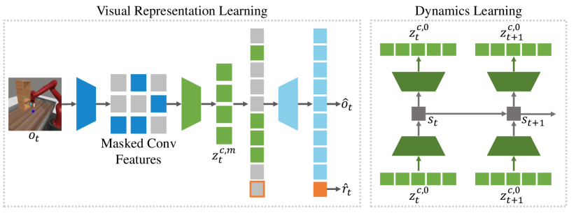
Figure 1: Illustration of our approach. We continually update visual representations and dynamics using online samples collected from environment interaction, by repeating iterative processes of training (Left) an autoencoder with convolutional feature masking and reward prediction and (Right) a latent dynamics model in the latent space of the autoencoder. We note that autoencoder parameters are not updated during dynamics learning.

Contributions

We highlight the contributions of our paper below:

• We demonstrate the effectiveness of decoupling visual representation learning and dynamics learning for visual model-based RL. MWM significantly outperforms a state-of-the-art model-based baseline [15] on various visual control tasks from Meta-world [16] and RLBench [17].

• We show that a self-supervised ViT trained to reconstruct visual observations with convolutional feature masking can be effective for visual model-based RL. Interestingly, we find that masking convolutional features can be more effective than pixel patch masking [13], by allowing for capturing fine-grained details within patches. This is in contrast to the observation in Touvron et al. [18], where both perform similarly on the ImageNet classification task [19].

• We show that an auxiliary reward prediction task can significantly improve performance by encoding task-relevant information into visual representations.

2 Related Work

World models from visual observations

There have been several approaches to learn visual representations for model-based approaches via image reconstruction [6, 7, 8, 9, 10, 11, 15, 20, 21, 22], e.g., learning a video prediction model [6, 23] or a latent dynamics model [8, 9, 10]. This has been followed by a series of works that demonstrated the effectiveness of model-based approaches for solving video games [15, 24, 22] and visual robot control tasks [7, 21, 25, 26]. There also have been several works that considered different objectives, including bisimulation [27] and contrastive learning [28, 29, 30]. While most prior works optimize a single model to learn both visual representations and dynamics, we instead develop a framework that decouples visual representation learning and dynamics learning.

Self-supervised vision transformers

Self-supervised learning with vision transformers (ViT) [14] has been actively studied. For instance, Chen et al. [31] introduced MoCo-v3 which trains a ViT with contrastive learning. Caron et al. [32] introduced DINO which utilizes a self-distillation loss [33], and demonstrated that self-supervised ViTs contain information about the semantic layout of images. Training self-supervised ViTs with masked image modeling [13, 34, 35, 36, 37, 38, 39] has also been successful. In particular, He et al. [13] proposed a masked autoencoder (MAE) that reconstructs masked pixel patches with an asymmetric encoder-decoder architecture. Unlike MAE, we propose to randomly mask features from early convolutional layers [40] instead of pixel patches and demonstrate that self-supervised ViTs can also be effective for visual model-based RL.

We provide more discussion on related works in more detail in Appendix C.

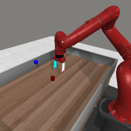
(a) Pick Place

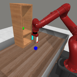
(b) Shelf Place

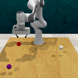
(c) Reach Target

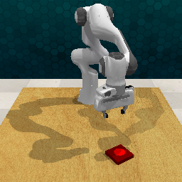
(d) Push Button

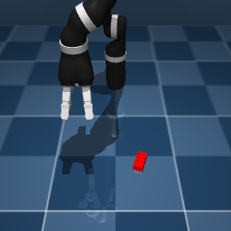
(e) Reach Duplo

Figure 2: Examples of visual observations used in our experiments. We consider a variety of visual robot control tasks from Meta-world [16], RLBench [17], and DeepMind Control Suite [41].

3 Preliminaries

Problem formulation

We formulate a visual control task as a partially observable Markov decision process (POMDP) [42], which is defined as a tuple $\left(\mathcal{O},\mathcal{A},p,r,\gamma\right)$. $\mathcal{O}$ is the observation space, $\mathcal{A}$ is the action space, $p\left(o_{t}|o_{<t},a_{<t}\right)$ is the transition dynamics, $r$ is the reward function that maps previous observations and actions to a reward $r_{t}=r\left(o_{\leq t},a_{<t}\right)$, and $\gamma\in[0,1)$ is the discount factor.

Dreamer

Dreamer [15, 21] is a visual model-based RL method that learns world models from pixels and trains an actor-critic model via latent imagination. Specifically, Dreamer learns a Recurrent State Space Model (RSSM) [9], which consists of following four components:

$$\begin{aligned} &\text{Representation model:}&&s_{t}\sim q_{\theta}(s_{t}\,|\,s_{t-1},a_{t-1},o_{t})&&\text{Image decoder:}&&\hat{o}_{t}\sim p_{\theta}(\hat{o}_{t}\,|\,s_{t})\\ &\text{Transition model:}&&\hat{s}_{t}\sim p_{\theta}(\hat{s}_{t}\,|\,s_{t-1},a_{t-1})&&\text{Reward predictor:}&&\hat{r}_{t}\sim p_{\theta}(\hat{r}_{t}\,|\,s_{t})\end{aligned}$$ (1)

The representation model extracts model state $s_{t}$ from previous model state $s_{t-1}$, previous action $a_{t-1}$, and current observation $o_{t}$. The transition model predicts future state $\hat{s}_{t}$ without the access to current observation $o_{t}$. The image decoder reconstructs raw pixels to provide learning signal, and the reward predictor enables us to compute rewards from future model states without decoding future frames. All model parameters $\theta$ are trained to jointly learn visual representations and environment dynamics by minimizing the negative variational lower bound [12]:

$$\begin{aligned} &\mathcal{L}(\theta)\doteq\mathbb{E}_{q_{\theta}\left(s_{1:T}|a_{1:T},o_{1:T}\right)}\Big{[}\\ &\textstyle\sum_{t=1}^{T}\Big{(}-\ln p_{\theta}(o_{t}|s_{t})-\ln p_{\theta}(r_{t}|s_{t})+\beta\,\text{KL}\left[q_{\theta}(s_{t}|s_{t-1},a_{t-1},o_{t})\,\|\,p_{\theta}(\hat{s}_{t}|s_{t-1},a_{t-1})\right]\Big{)}\Big{]},\end{aligned}$$ (2)

where $\beta$ is a hyperparameter that controls the tradeoff between the quality of visual representation learning and the accuracy of dynamics learning [43]. Then, the critic is learned to regress the values computed from imaginary rollouts, and the actor is trained to maximize the values by propagating analytic gradients back through the transition model (see Appendix A for the details).

Masked autoencoder

Masked autoencoder (MAE) [13] is a self-supervised visual representation technique that trains an autoencoder to reconstruct raw pixels with randomly masked patches consisting of pixels. Following a scheme introduced in vision transformer (ViT) [14], the observation $o_{t}\in\mathbb{R}^{H\times W\times C}$ is processed with a patchify stem that reshapes $o_{t}$ into a sequence of 2D patches $h_{t}\in\mathbb{R}^{N\times(P^{2}C)}$, where $P$ is the patch size and $N=HW/P^{2}$ is the number of patches. Then a subset of patches is randomly masked with a ratio of $m$ to construct $h^{m}_{t}\in\mathbb{R}^{M\times(P^{2}C)}$.

$$\begin{aligned} &\text{Patchify stem:}&&h_{t}=f^{\texttt{patch}}_{\phi}(o_{t})&&\text{Masking:}&&h_{t}^{m}\sim p^{\texttt{mask}}(h_{t}^{m}\,|\,h_{t},m)\end{aligned}$$ (3)

A ViT encoder embeds only the remaining patches $h^{m}_{t}$ into $D$-dimensional vectors, concatenates the embedded tokens with a learnable CLS token, and processes them through a series of Transformer layers [44]. Finally, a ViT decoder reconstructs the observation by processing tokens from the encoder and learnable mask tokens through Transformer layers followed by a linear output head:

$$\begin{aligned} &\text{ViT encoder:}&&z_{t}^{m}\sim p_{\phi}(z_{t}^{m}\,|\,h_{t}^{m})&&\text{ViT decoder:}&&\hat{o}_{t}\sim p_{\phi}(\hat{o}_{t}\,|\,z_{t}^{m})\end{aligned}$$ (4)

All the components paramaterized by $\phi$ are jointly optimized to minimize the mean squared error (MSE) between the reconstructed and original pixel patches. MAE computes $z^{0}_{t}$ without masking, and utilizes its first component (i.e., CLS representation) for downstream tasks (e.g., image classification).

4 Masked World Models

In this section, we present Masked World Models (MWM), a visual model-based RL framework for learning accurate world models by separately learning visual representations and environment dynamics. Our method repeats (i) updating an autoencoder with convolutional feature masking and an auxiliary reward prediction task (see Section 4.1), (ii) learning a dynamics model in the latent space of the autoencoder (see Section 4.2), and (iii) collecting samples from environment interaction. We provide the overview and pseudocode of MWM in Figure 1 and Appendix D, respectively.

4.1 Visual Representation Learning

It has been observed that masked image modeling with a ViT architecture [13, 34, 36] enables compute-efficient and stable self-supervised visual representation learning. This motivates us to adopt this approach for visual model-based RL, but we find that masked image modeling with commonly used pixel patch masking [13] often makes it difficult to learn fine-grained details within patches, e.g., small objects (see Appendix B for a motivating example). While one can consider small-size patches, this would increase computational costs due to the quadratic complexity of self-attention layers.

To handle this issue, we instead propose to train an autoencoder that reconstructs raw pixels given randomly masked convolutional features. Unlike previous approaches that utilize a patchify stem and randomly mask pixel patches (see Section 3), we adopt a convolution stem [14, 40] that processes $o_{t}$ through a series of convolutional layers followed by a flatten layer, to obtain $h^{c}_{t}\in\mathbb{R}^{N_{c}\times D}$ where $N_{c}$ is the number of convolutional features. Then $h^{c}_{t}$ is randomly masked with a ratio of $m$ to obtain $h^{c,m}_{t}\in\mathbb{R}^{M_{c}\times D}$, and ViT encoder and decoder process $h^{c,m}_{t}$ to reconstruct raw pixels.

$$\begin{aligned} &\text{Convolution stem:}&&h^{c}_{t}=f^{\texttt{conv}}_{\phi}(o_{t})&&\text{Masking:}&&h_{t}^{c,m}\sim p^{\texttt{mask}}(h_{t}^{c,m}\,|\,h^{c}_{t},m)\\ &\text{ViT encoder:}&&z_{t}^{c,m}\sim p_{\phi}(z_{t}^{c,m}\,|\,h_{t}^{c,m})&&\text{ViT decoder:}&&\hat{o}_{t}\sim p_{\phi}(\hat{o}_{t}\,|\,z_{t}^{c,m})\end{aligned}$$ (5)

Because early convolutional layers mix low-level details, we find that our autoencoder can effectively reconstruct all the details within patches by learning to extract information from nearby non-masked features (see Figure 7 for examples). This enables us to learn visual representations capturing such details while also achieving the benefits of MAE, e.g., stability and compute-efficiency.

Reward prediction

In order to encode task-relevant information that might not be captured solely by the reconstruction objective, we introduce an auxiliary objective for the autoencoder to predict rewards jointly with pixels. Specifically, we make the autoencoder predict the reward $r_{t}$ from $z_{t}^{c,m}$ in conjunction with raw pixels.

$$\begin{aligned} &\text{ViT decoder with reward prediction:}&&\hat{o}_{t},\hat{r}_{t}\sim p_{\phi}(\hat{o}_{t},\hat{r}_{t}\,|\,z_{t}^{c,m})\end{aligned}$$ (6)

In practice, we concatenate one additional learnable mask token to inputs of the ViT decoder, and utilize the corresponding output representation for predicting the reward with a linear output head.

High masking ratio

Introducing early convolutional layers might impede the masked reconstruction tasks because they propagate information across patches [18], and the model can exploit this to find a shortcut to solve reconstruction tasks. However, we find that a high masking ratio (i.e., 75%) can prevent the model from finding such shortcuts and induce useful representations (see Figure 6(b) for supporting experimental results). This also aligns with the observation from Touvron et al. [18], where masked image modeling [34] with a convolution stem [45] can achieve competitive performance with the patchify stem on the ImageNet classification task [19].

4.2 Latent Dynamics Learning

Once we learn visual representations, we leverage them for efficiently learning a dynamics model in the latent space of the autoencoder. Specifically, we obtain the frozen representations $z^{c,0}_{t}$ from the autoencoder, and then train a variant of RSSM whose inputs and reconstruction targets are $z^{c}_{t,0}$, by replacing the representation model and the image decoder in Equation 1 with following components:

$$\begin{aligned} &\text{Representation model:}&&s_{t}\sim q_{\theta}(s_{t}\,|\,s_{t-1},a_{t-1},z^{c,0}_{t})\\ &\text{Visual representation decoder:}&&\hat{z}^{c,0}_{t}\sim p_{\theta}(\hat{z}^{c,0}_{t}\,|\,s_{t})\end{aligned}$$ (7)

Because visual representations capture both high- and low-level information in an abstract form, the model can focus more on dynamics learning by reconstructing them instead of raw pixels (see Section 5.5 for relevant discussion). Here, we also note that we utilize all the elements of $z_{t}^{c,0}$ unlike MAE that only utilizes CLS representation for downstream tasks. We empirically find this enables the model to receive rich learning signals from reconstructing all the representations containing spatial information (see Appendix I for supporting experiments).

Optimization

Given a random batch $\{(o_{j},r_{j},a_{j})\}_{j=1}^{B}$, MWM objective is defined as follows:

$$\mathcal{L}^{\texttt{mwm}}(\phi,\theta)=\frac{1}{B}\sum_{j=1}^{B}\Big{(}\hskip 1.19995pt\underbracket{-\ln p_{\phi}(o_{j}|z^{c,m}_{j})-\ln p_{\phi}(r_{j}|z^{c,m}_{j})}_{\text{visual representation learning}}$$ (8)

$$\quad\quad\hskip 1.19995pt\underbracket{-\ln p_{\theta}(z^{c,0}_{j}|s_{j})-\ln p_{\theta}(r_{j}|s_{j})+\beta\,\text{KL}\left[q_{\theta}(s_{j}|s_{j-1},a_{j-1},z^{c,0}_{j})\,\|\,p_{\theta}(\hat{s}_{j}|s_{j-1},a_{j-1})\right]}_{\text{dynamics learning}}\Big{)}$$

5 Experiments

We evaluate MWM on various robotics benchmarks, including Meta-world [16] (see Section 5.1), RLBench [17] (see Section 5.2), and DeepMind Control Suite [46] (see Section 5.3). We remark that these benchmarks consist of diverse and challenging visual robotic tasks. We also analyze algorithmic design choices in-depth (see Section 5.4) and provide a qualitative analysis of how our decoupling approach works by visualizing the predictions from the latent dynamics model (see Section 5.5).

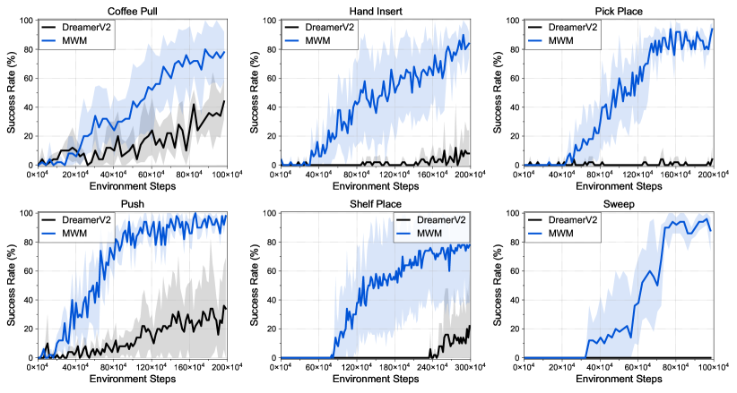
Figure 3: Learning curves on six visual robotic manipulation tasks from Meta-world as measured on the success rate. We select the tasks that require modeling interactions between small objects and robot arms. Learning curves on 50 tasks are available in Appendix G. The solid line and shaded regions represent the mean and bootstrap confidence intervals, respectively, across five runs.

Implementation

We use visual observations of $64\times 64\times 3$. For the convolution stem, we stack 3 convolution layers with the kernel size of 4 and stride 2, followed by a linear projection layer. We use a 4-layer ViT encoder and a 3-layer ViT decoder. We find that initializing the autoencoder with a warm-up schedule at the beginning of training is helpful. Unlike MAE, we compute the loss on entire pixels because we do not apply masking to pixels. For world models, we build our implementation on top of DreamerV2 [15]. To take a sequence of autoencoder representations as inputs, we replace a CNN encoder and decoder with a 2-layer Transformer encoder and decoder. We use same hyperparameters within the same benchmark. More details are available in Appendix E.

5.1 Meta-world Experiments

Environment details

In order to use a single camera viewpoint consistently over all 50 tasks, we use the modified corner2 camera viewpoint for all tasks. In our experiments, we classify 50 tasks into easy, medium, hard, and very hard tasks where experiments are run over 500K, 1M, 2M, 3M environments steps with action repeat of 2, respectively. More details are available in Appendix F.

Results

In Figure 3, we report the performance on a set of selected six challenging tasks that require agents to control robot arms to interact with small objects. We find that MWM significantly outperforms DreamerV2 in terms of both sample-efficiency and final performance. In particular, MWM achieves $>80\%$ success rate on Pick Place while DreamerV2 struggles to solve the task. These results show that our approach of separating visual representation learning and dynamics learning can learn accurate world models on challenging domains. We also note that DreamerV2 learns visual representations with the reward prediction loss, which implies that our superior performance does not come from utilizing additional information. Figure 4(a) shows the aggregate performance over all the 50 tasks from the benchmark, demonstrating that our method consistently outperforms DreamerV2 overall. We also provide learning curves on all individual tasks in Appendix G, where MWM consistently achieves similar or better performance on most tasks.

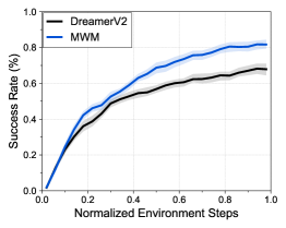
(a) Meta-world aggregated

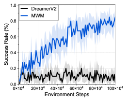
(b) RLBench: Reach Target

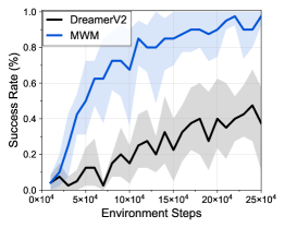
(c) RLBench: Push Button

Figure 4: (a) Aggregate performance on all 50 Meta-world tasks. We normalize environment steps by maximum steps in each task. The solid line and shaded regions represent the mean and stratified bootstrap confidence intervals, respectively, across 250 runs. We report the learning curves on (b) Reach Target and (c) Push Button from RLBench. Performances are not directly comparable to previous results [47, 48] due to the difference in setups (see Section 5.2). The solid line and shaded regions represent the mean and bootstrap confidence intervals, respectively, across eight runs.

5.2 RLBench Experiments

Environment details

In order to evaluate our method on more challenging visual robotic manipulation tasks, we consider RLBench [17], which has previously acted as an effective proxy for real-robot performance [48]. Since RLBench consists of sparse-reward and challenging tasks, solving them typically requires expert demonstrations, specialized network architectures, additional inputs (e.g., point cloud and proprioceptive states), and an action mode that requires path planning [47, 48, 49, 50]. While we could utilize some of these components, we instead leave this as future work in order to maintain a consistent evaluation setup across multiple domains. In our experiments, we instead consider two relatively easy tasks with dense rewards, and utilize an action mode that specifies the delta of joint positions. We provide more details in Appendix F.

Results

As shown in Figure 4(b) and Figure 4(c), we observe that our approach can also be effective on RLBench tasks, significantly outperforming DreamerV2. In particular, DreamerV2 achieves $<20\%$ success rate on Reach Target, while our approach can solve the tasks with $>80\%$ success rates. We find that this is because DreamerV2 fails to capture target positions in visual observations, while our method can capture such details (see Section 5.5 for relevant discussion and visualizations). However, we also note that these results are preliminary because they are still too sample-inefficient to be used for real-world scenarios. We provide more discussion in Section 6.

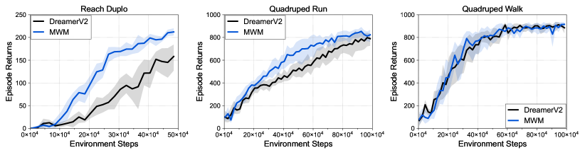
Figure 5: Learning curves on three visual robot control tasks from DeepMind Control Suite as measured on the episode return. The solid line and shaded regions represent the mean and bootstrap confidence intervals, respectively, across eight runs.

5.3 DeepMind Control Suite Experiments

Environment details

In order to demonstrate that our approach is generally applicable to diverse visual control tasks, we also evaluate our method on visual locomotion tasks from the widely used DeepMind Control Suite benchmark. Following a standard setup in Hafner et al. [21], we use an action repeat of 2 and default camera configurations. We provide more details in Appendix F.

Results

Figure 5 shows that our method achieves competitive performance to DreamerV2 on visual locomotion tasks (i.e., Quadruped tasks), demonstrating the generality of our approach across diverse visual control tasks. We also observe that our method outperforms DreamerV2 on Reach Duplo, which is one of a few manipulation tasks in the benchmark (see Figure 2(e) for an example). This implies that our method is effective on environments where the model should capture fine-grained details like object positions. More results are available in Appendix H, where trends are similar.

5.4 Ablation Study

Convolutional feature masking

We compare convolutional feature masking with pixel masking (i.e., MAE) in Figure 6(a), which shows that convolutional feature masking significantly outperforms pixel masking. Both results are achieved with the reward prediction. This demonstrates that enabling the model to capture fine-grained details within patches can be important for visual control. We also report the performance with varying masking ratio $m\in\{0.25,0.5,0.75,0.9\}$ in Figure 6(b). As we discussed in Section 4.1, we find that $m=0.75$ achieves better performance than $m\in\{0.25,0.5\}$ because strong regularization can prevent the model from finding a shortcut from input pixels. However, we also find that too strong regularization (i.e., $m=0.9$) degrades the performance.

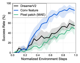
(a) Feature masking

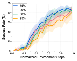
(b) Masking ratio

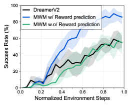
(c) Reward prediction

Figure 6: Learning curves on three manipulation tasks from Meta-world that investigate the effect of (a) convolutional feature masking, (b) masking ratio, and (c) reward prediction. The solid line and shaded regions represent the mean and stratified bootstrap confidence interval across 12 runs.

Figure 7: Future frames reconstructed with the autoencoder (i.e., Recon) and predicted by latent dynamics models (i.e., Predicted). Best viewed as video provided in Appendix B.

Reward prediction

In Figure 6(c), we find that performance significantly degrades without reward prediction, which shows that the reconstruction objective might not be sufficient for learning task-relevant information. It would be an interesting future direction to develop a representation learning scheme that learns task-relevant information without rewards because they might not be available in practice. We provide more ablation studies and learning curves on individual tasks in Appendix I. Moreover, we also show that reward prediction allows for learning useful representations that can be generally applicable to diverse robotic manipulation tasks in Appendix L.

5.5 Qualitative Analysis

We visually investigate how our world model works compared to the world model of DreamerV2. Specifically, we visualize the future frames predicted by latent dynamics models on Reach Target from RLBench in Figure 7. In this task, a robot arm should reach a target position specified by a red block in visual observations (see Figure 2(c)), which changes every trial. Thus it is crucial for the model to accurately predict the position of red blocks for solving the tasks. We find that our world model effectively captures the position of red blocks, while DreamerV2 fails. Interestingly, we also observe that our latent dynamics model ignores the components that are not task-relevant such as blue and orange blocks, though the reconstructions from the autoencoder are capturing all the details. This shows how our decoupling approach works: it encourages the autoencoder to focus on learning representations capturing the details and the dynamics model to focus on modeling task-relevant components of environments. We provide more examples in Appendix B.

6 Discussion

We have presented Masked World Models (MWM), which is a visual model-based RL framework that decouples visual representation learning and dynamics learning. By learning a latent dynamics model operating in the latent space of a self-supervised ViT, we find that our approach allows for solving a variety of visual control tasks from Meta-world, RLBench, and DeepMind Control Suite.

Limitation

Despite the results, there are a number of areas for improvement. As we have shown in Figure 6(c), the performance of our approach heavily depends on the auxiliary reward prediction task. This might be because our autoencoder is not learning temporal information, which is crucial for learning task-relevant information. It would be interesting to investigate the performance of video representation learning with ViTs [36, 51, 52]. It would also be interesting to study introducing auxiliary prediction for other modalities, such as audio. Another weakness is that our model operates only on RGB pixels from a single camera viewpoint; we look forward to a future work that incorporates different input modalities such as proprioceptive states and point clouds, building on top of the recent multi-modal learning approaches [53, 54]. Finally, our approach trains behaviors from scratch, which makes it still too sample-inefficient to be used in real-world scenarios. Leveraging a small number of demonstrations, incorporating the action mode with path planning [47], or pre-training a world model on video datasets [55] are directions we hope to investigate in future works.

Acknowledgments

We would like to thank Jongjin Park and Sihyun Yu for helpful discussions. We also thank Cirrascale Cloud Services for providing compute resources. This work was partially supported by National Science Foundation under grant NSF NRI #2024675, Office of Naval Research under grant N00014-21-1-2769 and grant N00014-22-1-2121, the Darpa RACER program, the Hong Kong Centre for Logistics Robotics, BMW, and Institute of Information & Communications Technology Planning & Evaluation (IITP) grant funded by the Korea government (MSIT) (No.2019-0-00075, Artificial Intelligence Graduate School Program (KAIST)).

Appendix

Appendix A Behavior Learning

We utilize the actor-critic learning scheme of DreamerV2 [15]. Specifically, we introduce a stochastic actor and a deterministic critic as below:

$$\begin{aligned} &\text{Actor:}&&\hat{a}_{t}\sim p_{\psi}(\hat{a}_{t}\,|\,\hat{s}_{t})&&\text{Critic:}&&v_{\xi}(\hat{s}_{t})\approx\mathbb{E}_{p_{\theta}}\left[\textstyle\sum_{i\leq t}\gamma^{i-t}\hat{r}_{i}\right],\end{aligned}$$ (9)

where {$\hat{s}_{t}$, $\hat{a}_{t}$, $\hat{r}_{t}$} is imagined future states, actions, and rewards which are recursively obtained by conditioning on a initial state $\hat{s}_{0}$ and utilizing the transition model and the reward model in Equation 1, and the actor in Equation 9. Note that the initial state $\hat{s}_{0}$ is the model state obtained from the representation model in Equation 1 using the samples from the replay buffer. Then the critic is trained to regress the $\lambda$-target [42, 56] as follows:

$$\mathcal{L}^{\texttt{critic}}(\xi)\doteq\mathbb{E}_{p_{\theta}}\left[\sum^{H-1}_{t=1}\frac{1}{2}\left(v_{\xi}(\hat{s}_{t})-\text{sg}(V_{t}^{\lambda})\right)^{2}\right],$$ (10)

$$V_{t}^{\lambda}\doteq\hat{r}_{t}+\gamma\begin{cases}(1-\lambda)v_{\xi}(\hat{s}_{t+1})+\lambda V_{t+1}^{\lambda}&\text{if}\ t<H\\ v_{\xi}(\hat{s}_{H})&\text{if}\ t=H,\end{cases}$$ (11)

where sg is a stop gradient function. Then we train the actor that maximizes the imagined return by back propagating the gradients through the learned world models as follows:

$$\mathcal{L}^{\texttt{actor}}(\psi)\doteq\mathbb{E}_{p_{\theta}}\left[-V_{t}^{\lambda}-\eta\,\text{H}\left[a_{t}|\hat{s}_{t}\right]\right],$$ (12)

where the entropy of actor $\,\text{H}\left[a_{t}|\hat{s}_{t}\right]$ is maximized to encourage exploration, and $\eta$ is a hyperparameter that adjusts the strength of entropy regularization. We refer to Hafner et al. [15] for more details.

Appendix B Extended Qualitative Analysis

We provide our qualitative analysis in videos on our project website:

https://sites.google.com/view/mwm-rl

which contains videos for (i) reconstructions from masked autoencoders (MAE) [13] and (ii) predictions from latent dynamics models. To be self-contained, we also provide reconstructions from masked autoencoders with images in Section B.1.

B.1 Reconstructions from Masked Autoencoders

In this section, we provide motivating examples for introducing convolutional feature masking. Specifically, we provide reconstructions from MAE [13] trained on Coffee-Pull and Peg-Insert-Side tasks from Meta-world [16] in Figure 8. We find that reconstruction with pixel patch masking can be an extremely difficult objective, which makes it difficult for the model to learn the fine-grained details such as object positions. For instance, in Figure 8, MAE struggles to predict the position of objects (e.g., a cup or a block) within masked patches, making it difficult to learn such details.

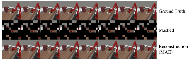
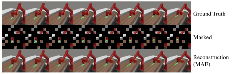
Figure 8: Frames reconstructed with the masked autoencoders (MAE) [13] trained on Meta-world (Top) Coffee Pull and (Bottom) Peg Insert Side. We find that reconstructions are not capturing the detailed object positions within patches. Best viewed as video provided in our website.

Appendix C Extended Related Work

Vision transformers with early convolution

Introducing convolutional layers into a ViT architecture is not new. Dosovitskiy et al. [14] investigated a hybrid ViT architecture that utilizes a modified version of ResNet [57] to obtain a convolutional feature map. This has been followed by a series of works that investigate the architecture design to introduce convolutions for improved performance [45, 58]. While these works mostly consider deep convolutional networks to maximize the performance on downstream tasks, we introduce a lightweight convolution stem consisting of a few convolution layers, following the design of Xiao et al. [40]. This is because our motivation for introducing the convolution stem is to avoid the pitfall of reconstruction objective with masked pixel patches, but not to investigate the optimal hybrid ViT architecture that maximizes the performance.

Convolutional feature masking

In the context of semantic segmentation, Dai et al. [59] proposed to utilize convolutional feature masking instead of pixel masking. But this differs in that their goal is to utilize the masks as inputs to classifiers, unlike our approach that drops convolutional features with masks. More related to our work is the approaches that mask out convolutional features as a regularization technique [60, 61]. For instance, Tompson et al. [60] demonstrated that masking out entire channels for a specific feature from a convolutional feature map can be more effective than Dropout [62] that masks randomly sampled channels. Ghiasi et al. [61] further developed this idea by proposing DropBlock that masks contiguous region of a feature map. In the context of visual control, Park et al. [63] trained a VQ-VAE [64] and proposed to drop convolutional features corresponding to randomly sampled discrete latent codes. Our work extends the idea of masking out convolutional features to self-supervised learning with a ViT and demonstrates its effectiveness for representation learning in visual model-based RL.

Unsupervised representation learning for visual control

Following the work of Jaderberg et al. [65] that demonstrated the effectiveness of auxiliary unsupervised objectives for RL, a variety of unsupervised learning objectives have been studied, including future latent reconstruction [27, 66, 67, 68], bisimulation [69, 70], contrastive learning [71, 72, 73, 74, 75, 30, 76, 29, 77, 78], keypoint extraction [79, 80, 81, 82], world model learning [8, 9, 10, 55] and reconstruction [83, 84]. Recent approaches have also demonstrated that simple data augmentations can sometimes be effective even without such representation learning objectives [85, 86, 87]. The work closest to ours is Xiao et al. [88], which demonstrated that frozen representations from MAE pre-trained on real-world videos can be used for training RL agents on visual manipulation tasks. Our work differs in that we demonstrate that training a self-supervised ViT with reconstruction and convolutional feature masking can be more effective for visual control tasks when compared to MAE that masks pixel patches. We also note that our work is orthogonal to Xiao et al. [88] in that our framework can also initialize the autoencoder with parameters pre-trained using real-world videos.

Appendix D Pseudocode

For clarity, we define the optimization objectives for autoencoder and latent dynamics model, and describe the pseudocode for our method. Specifically, given a random batch $\{(o_{j},r_{j},a_{j})\}_{j=1}^{B}$, visual representation learning and dynamics learning objectives are defined as:

$$\mathcal{L}^{\texttt{vis}}(\phi)=\frac{1}{B}\sum_{j=1}^{B}\Big{(}-\ln p_{\phi}(o_{j}|z^{c,m}_{j})-\ln p_{\phi}(r_{j}|z^{c,m}_{j})\Big{)}$$ (13)

$$\mathcal{L}^{\texttt{dyn}}(\theta)=\frac{1}{B}\sum_{j=1}^{B}\Big{(}-\ln p_{\theta}(z^{c,0}_{j}|s_{j})-\ln p_{\theta}(r_{j}|s_{j})$$ (14)

$$\quad\quad\quad\quad\quad\quad\quad\quad+\beta\,\text{KL}\left[q_{\theta}(s_{j}|s_{j-1},a_{j-1},z^{c,0}_{j})\,\|\,p_{\theta}(\hat{s}_{j}|s_{j-1},a_{j-1})\right]\Big{)}$$

Algorithm 1 Masked World Models

1:  Initialize parameters of autoencoder $\phi$, latent dynamics model $\theta$, actor $\psi$, and critic $\xi$

2:  Initialize replay buffer $\mathcal{B}\leftarrow\emptyset$

3:  for each timestep $t$ do

4:     // Collect transitions

5:     Get autoencoder representation $z_{t}^{c,0}$

6:     Update model state $s_{t}\sim q_{\theta}(s_{t}|s_{t-1},a_{t-1},z_{t}^{c,0})$

7:     Sample action $a_{t}\sim p_{\psi}(a_{t}|s_{t})$

8:     Add transition to replay buffer $\mathcal{B}\leftarrow\mathcal{B}\cup\{(o_{t},a_{t},r_{t})\}$

9:     // Visual representation learning with reward prediction

10:     Sample random minibatch $\{(o,r)\}\sim\mathcal{B}$

11:     Update autoencoder by minimizing $\mathcal{L}^{\texttt{vis}}(\phi)$

12:     // Dynamics learning

13:     Sample random minibatch $\{(o,r,a)\}\sim\mathcal{B}$

14:     Update latent dynamics model by minimizing $\mathcal{L}^{\texttt{dyn}}(\theta)$ and obtain states $\{s\}$

15:     // Actor Critic learning

16:     Imagine future rollouts $\{\hat{s},\hat{a},\hat{r}\}$ from $\{s\}$ using latent dynamics model and actor

17:     Update actor by minimizing $\mathcal{L}^{\texttt{actor}}(\psi)$

18:     Update critic by minimizing $\mathcal{L}^{\texttt{critic}}(\xi)$

19:  end for

Appendix E Architecture Details

E.1 Autoencoder

Convolution stem and masking

We use visual observations of $64\times 64\times 3$. For the convolution stem, similar to the design of Xiao et al. [40], we stack 3 convolution layers with the kernel size of $4\times 4$ and stride 2, followed by a convolution layer with the kernel size of $1\times 1$. This convolution stem processes $o_{t}$ into $8\times 8\times 256$, which has the same spatial shape of $8\times 8$ when we use the patchify stem with patch size of $8\times 8$. Then a masking is applied with a masking ratio of $m=0.75$.

ViT encoder and decoder

We use a 4-layer ViT encoder and a 3-layer ViT decoder, which are implemented using tfimm library. The ViT encoder concatenates class token with un-masked convolutional features, embeds inputs into 256-dimensional vectors, and processes them through Transformer layers. Then the ViT decoder takes outputs from the encoder and concatenate learnable mask tokens into them. Here, we use the same learnable mask token for reward prediction, which can be discriminated from other mask tokens because it gets different positional encoding. Finally, two linear output heads for predicting pixels and rewards are used to generate predictions. Unlike MAE, we compute the loss on entire pixels because we do not apply masking to pixels.

Initialization with warm-up schedule

We initialize parameters of the autoencoder using $5000$ gradients steps with a linear warm-up schedule over initial $2500$ steps using the samples collected from initial random exploration. We find this improves sample-efficiency on relatively easy tasks, but does not make significant difference on complex tasks. This is because better visual representations are used for learning latent dynamics models from the beginning. However, we also observe that this initialization is not required when we update the parameters in a more short interval (e.g., every 2 timesteps instead of 5 timesteps), because the autoencoder can be trained quickly without introducing such an initialization period. In our experiments, we use the initialization scheme and update the parameters every 5 timesteps for faster experimentation.

E.2 Latent Dynamics Model

Architecture

Our model is built upon the discrete latent dynamics model introduced in DreamerV2. Inputs to our model are representations $z_{t}^{c,0}$ from the autoencoder, which are of shape $8\times 8\times 256$ obtained by processing the visual observations through the convolution stem and ViT encoder of our autoencoder without masking (i.e., $m=0$). Because our dynamics model does not take visual observations as inputs, we do not utilize CNN encoder and decoder as in the original architecture. Instead, we introduce a shallow 2-layer ViT encoder and decoder with the embedding size of 128, which takes $z_{t}^{c,0}$ as inputs. Following Seo et al. [55], we increase the hidden size of dense layers and the model state dimension from 200 to 1024.

Prediction visualization

While the latent dynamics model is not trained directly to reconstruct raw pixels, its predictions can still be used for visualizing the open-loop predictions. This is because it is trained to reconstruct $z_{t}^{c,0}$, which can be processed through the ViT decoder of the autoencoder. We use this scheme for visualizing the predictions from the model in Figure 7.

Appendix F Experiments Details

Meta-world experiments

In order to use a single camera viewpoint consistently over all 50 tasks, we use the modified corner2 camera viewpoint for all tasks. Specifically, we adjusted the camera position with env.model.cam_pos[2][:]=[0.75, 0.075, 0.7], rendering visual observations as in Figure 2 which enables us to solve non-zero success rate on all tasks. Maximum episode length for Meta-world tasks is 500. We use the action repeat of 2, which we find it easy to solve tasks compared to the action repeat of 1 used in Seo et al. [55].

In our experiments, we classify 50 tasks into easy, medium, hard, and very hard tasks where experiments are run over 500K, 1M, 2M, 3M environments steps with action repeat of 2, respectively.

Difficulty	Tasks
easy	Button Press, Button Press Topdown, Button Press Topdown Wall, Button Press Wall, Coffee Button, Dial Turn, Door Close, Door Lock, Door Open, Door Unlock, Drawer Close, Drawer Open, Faucet Close, Faucet Open, Handle Press, Handle Press Side, Handle Pull, Handle Pull Side, Lever Pull, Plate Slide, Plate Slide Back, Plate Slide Back Side, Plate Slide Side, Reach, Reach Wall, Window Close, Window Open, Peg Unplug Side
medium	Basketball, Bin Picking, Box Close, Coffee Pull, Coffee Push, Hammer, Peg Insert Side, Push Wall, Soccer, Sweep, Sweep Into
hard	Assembly, Hand Insert, Pick Out of Hole, Pick Place, Push, Push Back
very hard	Shelf Place, Disassemble, Stick Pull, Stick Push, Pick Place Wall

RLBench experiments

We consider two relatively easy tasks (i.e., Reach Target and Push Button) with dense rewards, and utilize an action mode that specifies the delta of joint positions. Because original RLBench repository does not support shaped rewards for Push Button task, we design a shaped rewards for Push Button following the design of rewards in Reach Target. Specifically, the reward is defined as the sum of (i) the L2 distance of gripper to a button and (ii) the magnitude of the button being pushed. We set the maximum episode length to 200, and use the action repeat of 2. Because RLBench is designed to be episodic unlike Meta-world, we use the discount prediction scheme in DreamerV2 that introduces a linear head that predicts the termination of each rollout. For visual observations, we use the front RGB observation (see Figure 2 for an example).

DeepMind Control Suite experiments

We follow the setup of Hafner et al. [21] where the action repeat of 2 is used. We use default camera configurations without modification. We note that direct comparison with the results from Hafner et al. [21] is not possible because our experiments are based on DreamerV2 with larger networks (see Section E.2 for architecture details).

Computation

In terms of parameter counts, MWM consists of 25.9M parameters while DreamerV2 consists of 33.2M parameters. However, in terms of training time, MWM takes 5.5 hours for training over 500K environment steps, which is 1.57 times slower than DreamerV2 that takes 3.5 hours, because MWM processes visual observations through low-throughput ViT twice with and without masking. Given the improvement in final performances and sample-efficiency on complex tasks as demonstrated in our experiments, we note that it is worth spending additional computational costs.

Hyperparameters

We report the hyperparameters used in our experiments in Table 1.

Table 1: Hyperparameters used in our experiments. Unless otherwise specified, we use the same hyperparameters used in DreamerV2 [15]. DMC is an abbreviation of DeepMind Control Suite.

Hyperparameter	Value
Image observation	$64\times 64\times 3$
Image normalization	Mean: $(0.485,0.456,0.406)$, Std: $(0.229,0.224,0.225)$
Action repeat	$2$
Max episode length	$500$ (Meta-world), $200$ (RLBench), $1000$ (DMC)
Early episode termination	True (RLBench), False otherwise
Random exploration	$5000$ environment steps
Reward normalization	False (DMC), True otherwise
World model batch size	$16$ (DMC), $50$ otherwise
World model sequence length	$50$
World model tradeoff ($\beta$)	$0.1$ (RLBench), $1.0$ otherwise
World model tradeoff free-bits	$0.1$ (RLBench), $0.01$ otherwise
World model ViT encoder size	$2$ layers, $4$ heads, 128 units
World model ViT decoder size	$2$ layers, $4$ heads, 128 units
Autoencoder batch size	$1024$
Autoencoder initialization steps	$5000$
Autoencoder warm-up steps	$2500$
Autoencoder learning rate	$3\cdot 10^{-4}$
Autoencoder masking ratio	$0.75$
Autoencoder ViT encoder size	$4$ layers, 4 heads, 256 units
Autoencoder ViT decoder size	$3$ layers, 4 heads, 256 units

Appendix G Full Meta-world Experiments

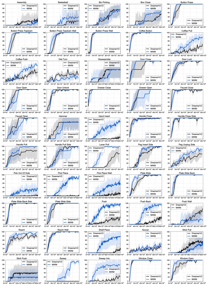
Figure 9: Learning curves on 50 visual robotic manipulation tasks from Meta-world as measured on the success rate. The solid line and shaded regions represent the mean and bootstrap confidence intervals, respectively, across five runs.

Appendix H Additional DeepMind Control Suite Experiments

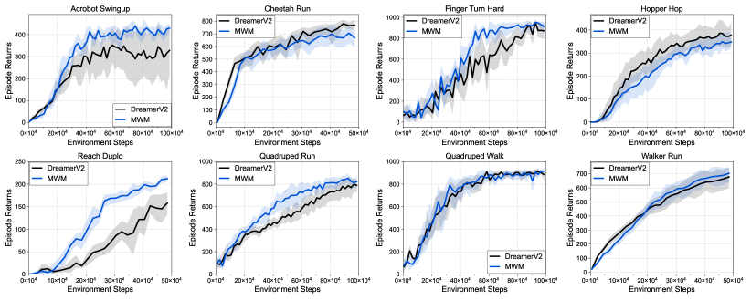
Figure 10: Learning curves on eight visual robot tasks from DeepMind Control Suite as measured on the episode return. The solid line and shaded regions represent the mean and bootstrap confidence intervals, respectively, across eight runs.

Appendix I Extended Ablation Study and Analysis

We provide additional analysis in Figure 11 and learning curves on individual tasks in Figure 12.

Utilizing only CLS representation

We ablate our design choice of utilizing all representations of $z_{t}^{c,0}$ for dynamics learning, instead of using only CLS representation as in MAE. As shown in Figure 11(a), we find that utilizing all representations (i.e., CLS + Conv) outperforms the baseline (i.e., CLS), by encouraging the model to learn spatial information included in all representations.

Model size

We report the performance of our method with varying number of layers for autoencoders in Figure 11(b). We find that there are no significant differences between three models sizes we consider, which might be because Meta-world visual observations are not too complex. It would be interesting to investigate the effect of model sizes in more complex environments.

DreamerV2 with ViT

In order to demonstrate that performance gain from our approach does not solely come from employing ViT instead of CNN, we evaluate DreamerV2 w/ ViT that replaces CNN encoder and decoder with ViT encoder and decoder, in Figure 11(c). We find DreamerV2 w/ ViT exhibits severe instability during training, and sometimes becomes completely unable to solve the tasks. We conjecture this might be because ViT suffers from unstable training without large data and regularization [14], which makes it difficult to learn world models end-to-end.

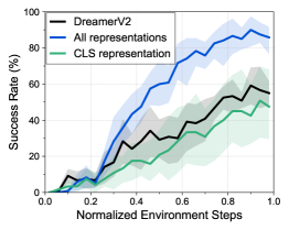
(a) Inputs to world models

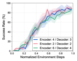
(b) Model size

(c) DreamerV2 with ViT

Figure 11: Learning curves on three manipulation tasks from Meta-world that investigate the effect of (a) inputs to world models and (b) autoencoder model sizes. (c) We also report the performance of DreamerV2 with CNNs and ViT. The solid line and shaded regions represent the mean and stratified bootstrap confidence interval across 12 runs.

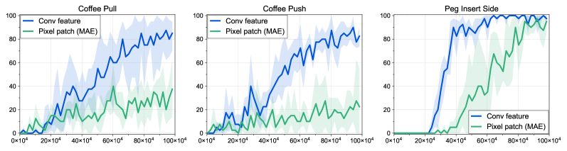
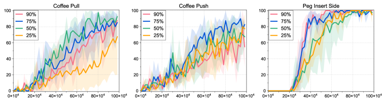
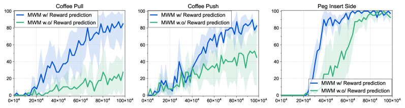
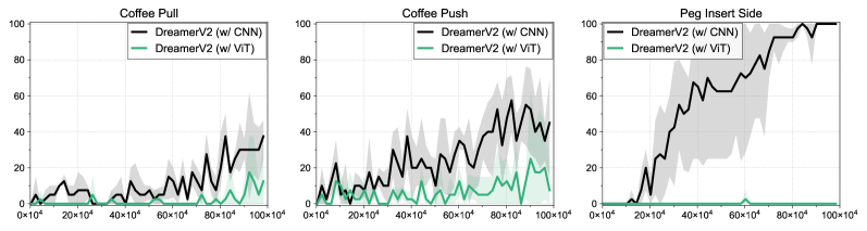
Figure 12: Learning curves on individual tasks used in ablation studies and analysis. The solid line and shaded regions represent the mean and bootstrap confidence interval across 4 runs.

Appendix J Additional Meta-world Experiments with Longer Environment Steps

We provide additional experiments that investigate the performance of DreamerV2 and MWM with more samples in Figure 13. Specifically, we report the performance of DreamerV2 over 6M environment steps, and find that DreamerV2 cannot outperform MWM even with much larger number of samples. This shows our approach allows for solving the tasks in a sample-efficient way with better asymptotic performance.

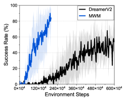
(a) Hand Insert

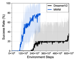
(b) Shelf Place

Figure 13: Learning curves on (a) Hand Insert and (b) Shelf Place tasks from Meta-world as measured on the success rate. The solid line and shaded regions represent the mean and bootstrap confidence intervals, respectively, across five runs.

Appendix K Comparison with Additional Baselines

In this section, we provide additional experiments that compare MWM with additional baselines. Specifically, we compare MWM against (i) a baseline that decouples visual representation and dynamics learning by learning the model on top of frozen VAE [12] representations and (ii) a baseline that learns representations via contrastive learning [9] instead of reconstruction in Figure 14.

Comparison with VAE

We find that the decoupled baseline based on VAE fails to solve most of the tasks, while MWM solves the target tasks. This shows that our representation learning method is crucial for performance improvement from the decoupling approach. It would be an interesting investigation to consider additional baselines that extracts keypoints and learns a dynamics model on top of them [79, 80, 81, 82].

Comparison with contrastive baseline

Moreover, we also observe that DreamerV2 with contrastive representation learning outperforms DreamerV2 with reconstruction, which shows that contrastive learning could be better in capturing fine-grained details from small objects. But importantly we find MWM still outperforms DreamerV2 (Contrastive) especially on Pick Place task, which demonstrates the effectiveness of our decoupled approach for solving challenging manipulation tasks.

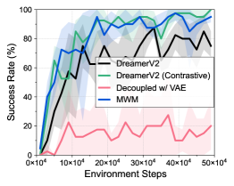
(a) Reach

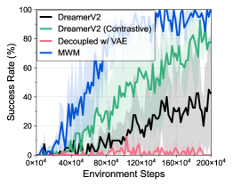
(b) Push

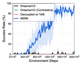
(c) Pick Place

Figure 14: Learning curves on (a) Reach, (b) Push, and (c) Pick Place tasks from Meta-world as measured on the success rate. The solid line and shaded regions represent the mean and bootstrap confidence intervals, respectively, across four runs.

Appendix L Generalizability of Representations Learned with Reward Prediction

As we mentioned in Section 6, representation learning only with task-irrelevant information would be an interesting direction to further improve the applicability of our approach to diverse setups. Nevertheless, we remark that reward prediction on a specific task can also encourage visual representations to capture task-irrelevant information useful for solving various manipulation tasks. For instance, rewards are often designed to contain information about robot arm movements (e.g., translations and rotations) and fine-grained details about objects, which can be shared across various tasks.

Transfer to unseen tasks

In order to empirically support this, we report the experimental results where we utilize frozen representations trained on Push task for solving manipulation tasks with a difference to push task: (i) Push Back that requires moving a block to a different position, (ii) Pick Place that requires picking up the block, and (iii) Drawer Open that contains unseen drawer object in the observation. As shown in Figure 15, we observe that performance with frozen representations from unseen task can be similar to or better than the performance of MWM trained from scratch, which shows that representations learned with reward prediction can be versatile.

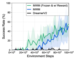
(a) Pick Place

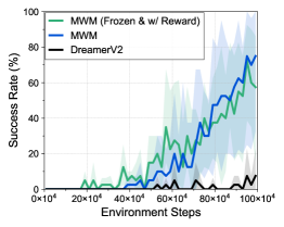
(b) Push Back

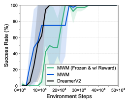
(c) Drawer Open

Figure 15: Learning curves on (a) Pick Place, (b) Push Back, and (c) Drawer Open tasks from Meta-world as measured on the success rate. The solid line and shaded regions represent the mean and bootstrap confidence intervals, respectively, across four runs.

State regression analysis

To further investigate how reward prediction affects the quality of learned representations, we provide additional experiments where we train a regression model to predict proprioceptive states available from the simulator. Specifically, we first train MWM on Meta-world Push task with and without reward prediction, and train a regression model to predict the states in Push (seen) and Pick-place (unseen) tasks on top of frozen autoencoder representations from Push task. In Figure 16, we observe that representations trained with reward prediction consistently achieve low prediction error. This supports that reward prediction can indeed provide useful information for robotic manipulation.

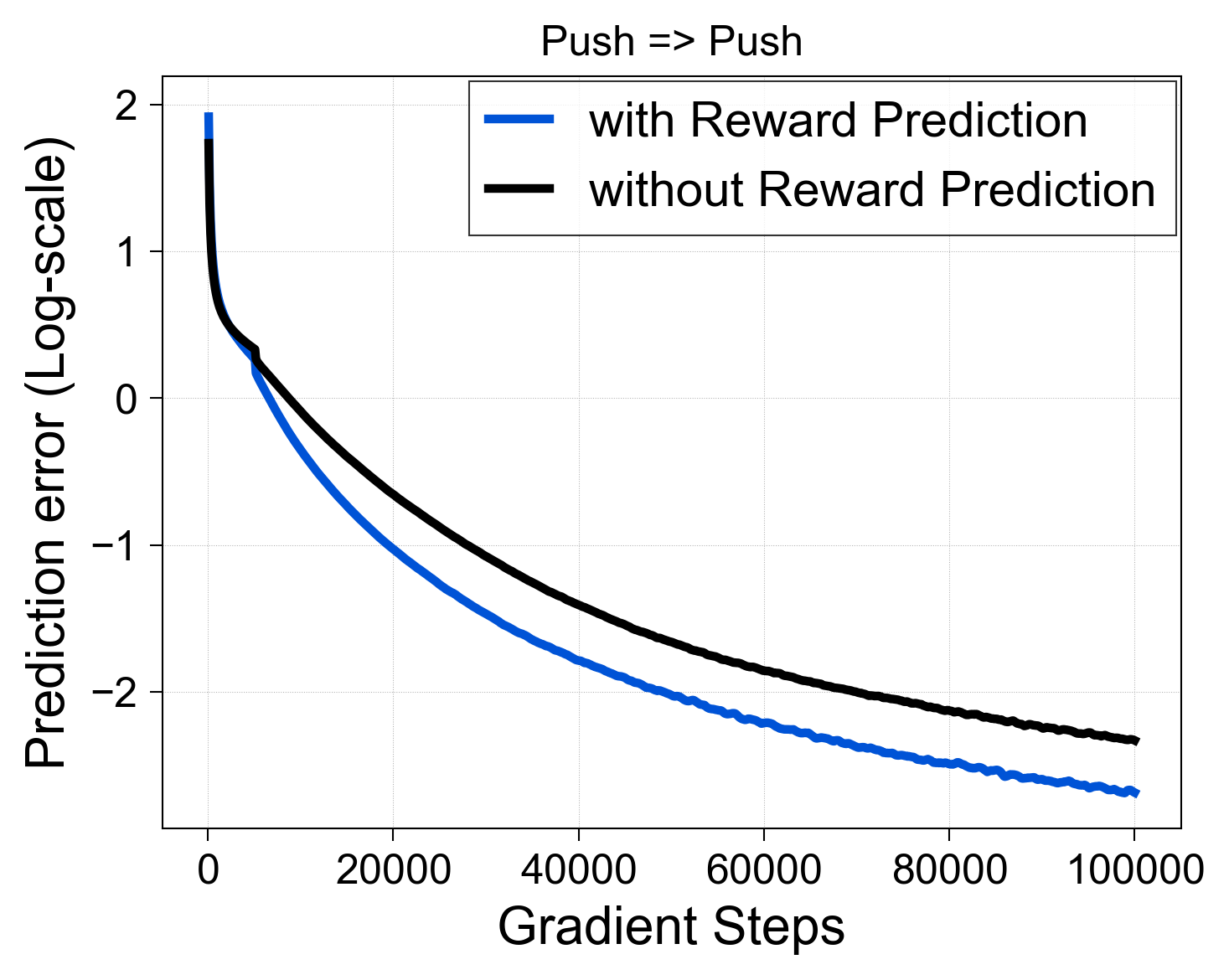
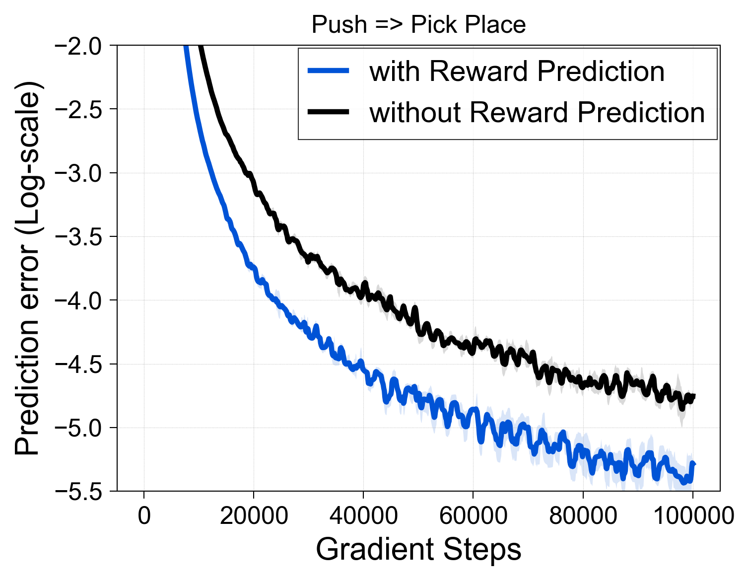
Figure 16: Learning curves of regression models that predicts proprioceptive states using the frozen representations pre-trained from Push task on (a) Push and (b) Pick Place tasks. The solid line and shaded regions represent the mean and bootstrap confidence intervals, respectively, across four runs.

References

- Chua et al. [2018] K. Chua, R. Calandra, R. McAllister, and S. Levine. Deep reinforcement learning in a handful of trials using probabilistic dynamics models. In Advances in neural information processing systems, 2018.
- Deisenroth and Rasmussen [2011] M. Deisenroth and C. E. Rasmussen. Pilco: A model-based and data-efficient approach to policy search. In International Conference on Machine Learning, 2011.
- Lenz et al. [2015] I. Lenz, R. A. Knepper, and A. Saxena. Deepmpc: Learning deep latent features for model predictive control. In Robotics: Science and Systems, 2015.
- Kurutach et al. [2018] T. Kurutach, I. Clavera, Y. Duan, A. Tamar, and P. Abbeel. Model-ensemble trust-region policy optimization. In International Conference on Learning Representations, 2018.
- Janner et al. [2019] M. Janner, J. Fu, M. Zhang, and S. Levine. When to trust your model: Model-based policy optimization. Advances in Neural Information Processing Systems, 2019.
- Finn and Levine [2017] C. Finn and S. Levine. Deep visual foresight for planning robot motion. In 2017 IEEE International Conference on Robotics and Automation (ICRA), 2017.
- Ebert et al. [2018] F. Ebert, C. Finn, S. Dasari, A. Xie, A. Lee, and S. Levine. Visual foresight: Model-based deep reinforcement learning for vision-based robotic control. arXiv preprint arXiv:1812.00568, 2018.
- Watter et al. [2015] M. Watter, J. Springenberg, J. Boedecker, and M. Riedmiller. Embed to control: A locally linear latent dynamics model for control from raw images. In Advances in neural information processing systems, 2015.
- Hafner et al. [2019] D. Hafner, T. Lillicrap, I. Fischer, R. Villegas, D. Ha, H. Lee, and J. Davidson. Learning latent dynamics for planning from pixels. In International Conference on Machine Learning, 2019.
- Zhang et al. [2019] M. Zhang, S. Vikram, L. Smith, P. Abbeel, M. Johnson, and S. Levine. Solar: Deep structured representations for model-based reinforcement learning. In International Conference on Machine Learning, 2019.
- Ha and Schmidhuber [2018] D. Ha and J. Schmidhuber. World models. In Advances in Neural Information Processing Systems, 2018.
- Kingma and Welling [2014] D. P. Kingma and M. Welling. Auto-encoding variational bayes. In International Conference on Learning Representations, 2014.
- He et al. [2021] K. He, X. Chen, S. Xie, Y. Li, P. Dollár, and R. Girshick. Masked autoencoders are scalable vision learners. arXiv preprint arXiv:2111.06377, 2021.
- Dosovitskiy et al. [2021] A. Dosovitskiy, L. Beyer, A. Kolesnikov, D. Weissenborn, X. Zhai, T. Unterthiner, M. Dehghani, M. Minderer, G. Heigold, S. Gelly, et al. An image is worth 16x16 words: Transformers for image recognition at scale. In International Conference on Learning Representaitons, 2021.
- Hafner et al. [2021] D. Hafner, T. Lillicrap, M. Norouzi, and J. Ba. Mastering atari with discrete world models. In International Conference on Learning Representations, 2021.
- Yu et al. [2020] T. Yu, D. Quillen, Z. He, R. Julian, K. Hausman, C. Finn, and S. Levine. Meta-world: A benchmark and evaluation for multi-task and meta reinforcement learning. In Conference on Robot Learning, 2020.
- James et al. [2020] S. James, Z. Ma, D. R. Arrojo, and A. J. Davison. RLBench: The robot learning benchmark & learning environment. IEEE Robotics and Automation Letters, 2020.
- Touvron et al. [2022] H. Touvron, M. Cord, A. El-Nouby, J. Verbeek, and H. Jégou. Three things everyone should know about vision transformers. arXiv preprint arXiv:2203.09795, 2022.
- Deng et al. [2009] J. Deng, W. Dong, R. Socher, L.-J. Li, K. Li, and L. Fei-Fei. Imagenet: A large-scale hierarchical image database. In 2009 IEEE conference on computer vision and pattern recognition, 2009.
- Finn et al. [2016] C. Finn, X. Y. Tan, Y. Duan, T. Darrell, S. Levine, and P. Abbeel. Deep spatial autoencoders for visuomotor learning. In 2016 IEEE International Conference on Robotics and Automation (ICRA), 2016.
- Hafner et al. [2020] D. Hafner, T. Lillicrap, J. Ba, and M. Norouzi. Dream to control: Learning behaviors by latent imagination. In International Conference on Learning Representations, 2020.
- Kaiser et al. [2019] L. Kaiser, M. Babaeizadeh, P. Milos, B. Osinski, R. H. Campbell, K. Czechowski, D. Erhan, C. Finn, P. Kozakowski, S. Levine, et al. Model-based reinforcement learning for atari. In International Conference on Learning Representations, 2019.
- Gupta et al. [2022] A. Gupta, S. Tian, Y. Zhang, J. Wu, R. Martín-Martín, and L. Fei-Fei. Maskvit: Masked visual pre-training for video prediction. arXiv preprint arXiv:2206.11894, 2022.
- Ye et al. [2021] W. Ye, S. Liu, T. Kurutach, P. Abbeel, and Y. Gao. Mastering atari games with limited data. Advances in Neural Information Processing Systems, 2021.
- Seyde et al. [2021] T. Seyde, W. Schwarting, S. Karaman, and D. Rus. Learning to plan optimistically: Uncertainty-guided deep exploration via latent model ensembles. In Conference on Robot Learning, 2021.
- Rybkin et al. [2021] O. Rybkin, C. Zhu, A. Nagabandi, K. Daniilidis, I. Mordatch, and S. Levine. Model-based reinforcement learning via latent-space collocation. In International Conference on Machine Learning, 2021.
- Gelada et al. [2019] C. Gelada, S. Kumar, J. Buckman, O. Nachum, and M. G. Bellemare. Deepmdp: Learning continuous latent space models for representation learning. In International Conference on Machine Learning, 2019.
- Nguyen et al. [2021] T. D. Nguyen, R. Shu, T. Pham, H. Bui, and S. Ermon. Temporal predictive coding for model-based planning in latent space. In International Conference on Machine Learning, 2021.
- Okada and Taniguchi [2021] M. Okada and T. Taniguchi. Dreaming: Model-based reinforcement learning by latent imagination without reconstruction. In 2021 IEEE International Conference on Robotics and Automation (ICRA), 2021.
- Deng et al. [2021] F. Deng, I. Jang, and S. Ahn. Dreamerpro: Reconstruction-free model-based reinforcement learning with prototypical representations. arXiv preprint arXiv:2110.14565, 2021.
- Chen et al. [2021] X. Chen, S. Xie, and K. He. An empirical study of training self-supervised vision transformers. In Proceedings of the IEEE/CVF International Conference on Computer Vision, 2021.
- Caron et al. [2021] M. Caron, H. Touvron, I. Misra, H. Jégou, J. Mairal, P. Bojanowski, and A. Joulin. Emerging properties in self-supervised vision transformers. In Proceedings of the IEEE/CVF International Conference on Computer Vision, 2021.
- Hinton et al. [2015] G. Hinton, O. Vinyals, J. Dean, et al. Distilling the knowledge in a neural network. arXiv preprint arXiv:1503.02531, 2015.
- Bao et al. [2021] H. Bao, L. Dong, and F. Wei. Beit: Bert pre-training of image transformers. arXiv preprint arXiv:2106.08254, 2021.
- Li et al. [2021] Z. Li, Z. Chen, F. Yang, W. Li, Y. Zhu, C. Zhao, R. Deng, L. Wu, R. Zhao, M. Tang, et al. Mst: Masked self-supervised transformer for visual representation. In Advances in Neural Information Processing Systems, 2021.
- Feichtenhofer et al. [2022] C. Feichtenhofer, H. Fan, Y. Li, and K. He. Masked autoencoders as spatiotemporal learners. arXiv preprint arXiv:2205.09113, 2022.
- Xie et al. [2022] Z. Xie, Z. Zhang, Y. Cao, Y. Lin, J. Bao, Z. Yao, Q. Dai, and H. Hu. Simmim: A simple framework for masked image modeling. In Proceedings of the IEEE/CVF Conference on Computer Vision and Pattern Recognition, 2022.
- Wei et al. [2022] C. Wei, H. Fan, S. Xie, C.-Y. Wu, A. Yuille, and C. Feichtenhofer. Masked feature prediction for self-supervised visual pre-training. In Proceedings of the IEEE/CVF Conference on Computer Vision and Pattern Recognition, 2022.
- Zhou et al. [2021] J. Zhou, C. Wei, H. Wang, W. Shen, C. Xie, A. Yuille, and T. Kong. ibot: Image bert pre-training with online tokenizer. arXiv preprint arXiv:2111.07832, 2021.
- Xiao et al. [2021] T. Xiao, M. Singh, E. Mintun, T. Darrell, P. Dollár, and R. Girshick. Early convolutions help transformers see better. In Advances in Neural Information Processing Systems, 2021.
- Tassa et al. [2020] Y. Tassa, S. Tunyasuvunakool, A. Muldal, Y. Doron, S. Liu, S. Bohez, J. Merel, T. Erez, T. Lillicrap, and N. Heess. dm_control: Software and tasks for continuous control. arXiv preprint arXiv:2006.12983, 2020.
- Sutton and Barto [2018] R. S. Sutton and A. G. Barto. Reinforcement learning: An introduction. MIT Press, 2018.
- Alemi et al. [2018] A. Alemi, B. Poole, I. Fischer, J. Dillon, R. A. Saurous, and K. Murphy. Fixing a broken elbo. In International Conference on Machine Learning, 2018.
- Vaswani et al. [2017] A. Vaswani, N. Shazeer, N. Parmar, J. Uszkoreit, L. Jones, A. N. Gomez, Ł. Kaiser, and I. Polosukhin. Attention is all you need. In Advances in Neural Information Processing Systems, 2017.
- Graham et al. [2021] B. Graham, A. El-Nouby, H. Touvron, P. Stock, A. Joulin, H. Jégou, and M. Douze. Levit: a vision transformer in convnet’s clothing for faster inference. In Proceedings of the IEEE/CVF International Conference on Computer Vision, 2021.
- Tassa et al. [2012] Y. Tassa, T. Erez, and E. Todorov. Synthesis and stabilization of complex behaviors through online trajectory optimization. In International Conference on Intelligent Robots and Systems, 2012.
- James and Davison [2022] S. James and A. J. Davison. Q-attention: Enabling efficient learning for vision-based robotic manipulation. IEEE Robotics and Automation Letters, 2022.
- James et al. [2022] S. James, K. Wada, T. Laidlow, and A. J. Davison. Coarse-to-Fine Q-attention: Efficient learning for visual robotic manipulation via discretisation. Proceedings of the IEEE/CVF Conference on Computer Vision and Pattern Recognition, 2022.
- James and Abbeel [2022a] S. James and P. Abbeel. Coarse-to-Fine Q-attention with Learned Path Ranking. arXiv preprint arXiv:2204.01571, 2022a.
- James and Abbeel [2022b] S. James and P. Abbeel. Coarse-to-Fine Q-attention with Tree Expansion. arXiv preprint arXiv:2204.12471, 2022b.
- Tong et al. [2022] Z. Tong, Y. Song, J. Wang, and L. Wang. Videomae: Masked autoencoders are data-efficient learners for self-supervised video pre-training. In Advances in Neural Information Processing Systems, 2022.
- Arnab et al. [2021] A. Arnab, M. Dehghani, G. Heigold, C. Sun, M. Lučić, and C. Schmid. Vivit: A video vision transformer. In Proceedings of the IEEE/CVF International Conference on Computer Vision, 2021.
- Geng et al. [2022] X. Geng, H. Liu, L. Lee, D. Schuurams, S. Levine, and P. Abbeel. Multimodal masked autoencoders learn transferable representations. arXiv preprint arXiv:2205.14204, 2022.
- Bachmann et al. [2022] R. Bachmann, D. Mizrahi, A. Atanov, and A. Zamir. Multimae: Multi-modal multi-task masked autoencoders. arXiv preprint arXiv:2204.01678, 2022.
- Seo et al. [2022] Y. Seo, K. Lee, S. James, and P. Abbeel. Reinforcement learning with action-free pre-training from videos. In International Conference on Machine Learning, 2022.
- Schulman et al. [2015] J. Schulman, P. Moritz, S. Levine, M. Jordan, and P. Abbeel. High-dimensional continuous control using generalized advantage estimation. arXiv preprint arXiv:1506.02438, 2015.
- He et al. [2016] K. He, X. Zhang, S. Ren, and J. Sun. Deep residual learning for image recognition. In Proceedings of the IEEE conference on computer vision and pattern recognition, 2016.
- Wu et al. [2021] H. Wu, B. Xiao, N. Codella, M. Liu, X. Dai, L. Yuan, and L. Zhang. Cvt: Introducing convolutions to vision transformers. In Proceedings of the IEEE/CVF International Conference on Computer Vision, 2021.
- Dai et al. [2015] J. Dai, K. He, and J. Sun. Convolutional feature masking for joint object and stuff segmentation. In Proceedings of the IEEE conference on computer vision and pattern recognition, pages 3992–4000, 2015.
- Tompson et al. [2015] J. Tompson, R. Goroshin, A. Jain, Y. LeCun, and C. Bregler. Efficient object localization using convolutional networks. In Proceedings of the IEEE conference on computer vision and pattern recognition, 2015.
- Ghiasi et al. [2018] G. Ghiasi, T.-Y. Lin, and Q. V. Le. Dropblock: A regularization method for convolutional networks. Advances in neural information processing systems, 31, 2018.
- Srivastava et al. [2014] N. Srivastava, G. Hinton, A. Krizhevsky, I. Sutskever, and R. Salakhutdinov. Dropout: a simple way to prevent neural networks from overfitting. The journal of machine learning research, 2014.
- Park et al. [2021] J. Park, Y. Seo, C. Liu, L. Zhao, T. Qin, J. Shin, and T.-Y. Liu. Object-aware regularization for addressing causal confusion in imitation learning. In Advances in Neural Information Processing Systems, 2021.
- Van Den Oord et al. [2017] A. Van Den Oord, O. Vinyals, et al. Neural discrete representation learning. In Advances in Neural Information Processing Systems, 2017.
- Jaderberg et al. [2017] M. Jaderberg, V. Mnih, W. M. Czarnecki, T. Schaul, J. Z. Leibo, D. Silver, and K. Kavukcuoglu. Reinforcement learning with unsupervised auxiliary tasks. In International Conference on Learning Representations, 2017.
- Schwarzer et al. [2021] M. Schwarzer, A. Anand, R. Goel, R. D. Hjelm, A. Courville, and P. Bachman. Data-efficient reinforcement learning with self-predictive representations. In International Conference on Learning Representations, 2021.
- Yu et al. [2021] T. Yu, C. Lan, W. Zeng, M. Feng, Z. Zhang, and Z. Chen. Playvirtual: Augmenting cycle-consistent virtual trajectories for reinforcement learning. In Advances in Neural Information Processing Systems, 2021.
- Yu et al. [2022] T. Yu, Z. Zhang, C. Lan, Z. Chen, and Y. Lu. Mask-based latent reconstruction for reinforcement learning. arXiv preprint arXiv:2201.12096, 2022.
- Castro [2020] P. S. Castro. Scalable methods for computing state similarity in deterministic markov decision processes. In Proceedings of the AAAI Conference on Artificial Intelligence, 2020.
- Zhang et al. [2021] A. Zhang, R. McAllister, R. Calandra, Y. Gal, and S. Levine. Learning invariant representations for reinforcement learning without reconstruction. In International Conference on Learning Representations, 2021.
- Oord et al. [2018] A. v. d. Oord, Y. Li, and O. Vinyals. Representation learning with contrastive predictive coding. In Advances in Neural Information Processing Systems, 2018.
- Anand et al. [2019] A. Anand, E. Racah, S. Ozair, Y. Bengio, M.-A. Côté, and R. D. Hjelm. Unsupervised state representation learning in atari. In Advances in Neural Information Processing Systems, 2019.
- Mazoure et al. [2020] B. Mazoure, R. T. d. Combes, T. Doan, P. Bachman, and R. D. Hjelm. Deep reinforcement and infomax learning. In Advances in Neural Information Processing Systems, 2020.
- Srinivas et al. [2020] A. Srinivas, M. Laskin, and P. Abbeel. Curl: Contrastive unsupervised representations for reinforcement learning. In Internatial Conference on Machine Learning, 2020.
- Liu and Abbeel [2021] H. Liu and P. Abbeel. Behavior from the void: Unsupervised active pre-training. arXiv preprint arXiv:2103.04551, 2021.
- Yarats et al. [2021] D. Yarats, R. Fergus, A. Lazaric, and L. Pinto. Reinforcement learning with prototypical representations. In International Conference on Machine Learning, 2021.
- Nair et al. [2022] S. Nair, A. Rajeswaran, V. Kumar, C. Finn, and A. Gupta. R3m: A universal visual representation for robot manipulation. arXiv preprint arXiv:2203.12601, 2022.
- Parisi et al. [2022] S. Parisi, A. Rajeswaran, S. Purushwalkam, and A. Gupta. The unsurprising effectiveness of pre-trained vision models for control. arXiv preprint arXiv:2203.03580, 2022.
- Minderer et al. [2019] M. Minderer, C. Sun, R. Villegas, F. Cole, K. P. Murphy, and H. Lee. Unsupervised learning of object structure and dynamics from videos. In Advances in Neural Information Processing Systems, 2019.
- Manuelli et al. [2020] L. Manuelli, Y. Li, P. Florence, and R. Tedrake. Keypoints into the future: Self-supervised correspondence in model-based reinforcement learning. arXiv preprint arXiv:2009.05085, 2020.
- Lambeta et al. [2020] M. Lambeta, P.-W. Chou, S. Tian, B. Yang, B. Maloon, V. R. Most, D. Stroud, R. Santos, A. Byagowi, G. Kammerer, et al. Digit: A novel design for a low-cost compact high-resolution tactile sensor with application to in-hand manipulation. IEEE Robotics and Automation Letters, 2020.
- Das et al. [2021] N. Das, S. Bechtle, T. Davchev, D. Jayaraman, A. Rai, and F. Meier. Model-based inverse reinforcement learning from visual demonstrations. In Conference on Robot Learning, 2021.
- Yarats et al. [2021] D. Yarats, A. Zhang, I. Kostrikov, B. Amos, J. Pineau, and R. Fergus. Improving sample efficiency in model-free reinforcement learning from images. In Proceedings of the AAAI Conference on Artificial Intelligence, 2021.
- Shelhamer et al. [2016] E. Shelhamer, P. Mahmoudieh, M. Argus, and T. Darrell. Loss is its own reward: Self-supervision for reinforcement learning. arXiv preprint arXiv:1612.07307, 2016.
- Yarats et al. [2021] D. Yarats, R. Fergus, A. Lazaric, and L. Pinto. Mastering visual continuous control: Improved data-augmented reinforcement learning. arXiv preprint arXiv:2107.09645, 2021.
- Laskin et al. [2020] M. Laskin, K. Lee, A. Stooke, L. Pinto, P. Abbeel, and A. Srinivas. Reinforcement learning with augmented data. In Advances in Neural Information Processing Systems, 2020.
- Kostrikov et al. [2021] I. Kostrikov, D. Yarats, and R. Fergus. Image augmentation is all you need: Regularizing deep reinforcement learning from pixels. In International Conference on Learning Representations, 2021.
- Xiao et al. [2022] T. Xiao, I. Radosavovic, T. Darrell, and J. Malik. Masked visual pre-training for motor control. arXiv preprint arXiv:2203.06173, 2022.