Learning Symmetric Rules with SATNet
Abstract
SATNet is a differentiable constraint solver with a custom backpropagation algorithm, which can be used as a layer in a deep-learning system. It is a promising proposal for bridging deep learning and logical reasoning. In fact, SATNet has been successfully applied to learn, among others, the rules of a complex logical puzzle, such as Sudoku, just from input and output pairs where inputs are given as images. In this paper, we show how to improve the learning of SATNet by exploiting symmetries in the target rules of a given but unknown logical puzzle or more generally a logical formula. We present SymSATNet, a variant of SATNet that translates the given symmetries of the target rules to a condition on the parameters of SATNet and requires that the parameters should have a particular parametric form that guarantees the condition. The requirement dramatically reduces the number of parameters to learn for the rules with enough symmetries, and makes the parameter learning of SymSATNet much easier than that of SATNet. We also describe a technique for automatically discovering symmetries of the target rules from examples. Our experiments with Sudoku and Rubik’s cube show the substantial improvement of SymSATNet over the baseline SATNet.
1 Introduction
Bringing the ability of reasoning to the deep-learning systems has been the aim of a large amount of recent research efforts [Yang et al., 2017, Evans and Grefenstette, 2018, Cingillioglu and Russo, 2019, Wang et al., 2019, Topan et al., 2021]. One notable outcome of these endeavours is SATNet [Wang et al., 2019], a differentiable constraint solver with an efficient custom backpropagation algorithm. SATNet can be used as a component of a deep-learning system and make the system capable of learning and reasoning about sophisticated logical rules. Its potential has been demonstrated successfully with the tasks of learning the rules of complex logical puzzles, such as Sudoku, just from input-output examples where the inputs are given as images.
We show how to improve the rule (or constraint) learning of SATNet, when the target rules have permutation symmetries. By having symmetries, we mean the solutions of the rules are closed under the permutations of those symmetries. For example, in Sudoku, if a completed Sudoku board is a solution, permuting the numbers to in the board, the first three rows, or the last three columns always gives rise to another solution. Thus, these permutations are symmetries of Sudoku.
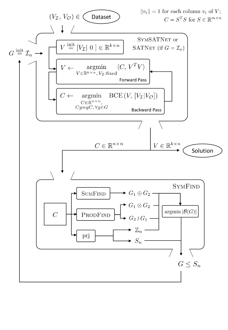
Our improvement is a variant of SATNet, called SymSATNet, which abbreviates symmetry-aware SATNet. SymSATNet assumes that some symmetries of the target rules are given a priori although the rules themselves are unknown. It then translates these symmetries into a condition on the parameter matrix of SATNet (or our minor generalisation), and requires that the parameters have a particular parametric form that guarantees the condition. Concretely, the translated condition says that the matrix regarded as a linear map should be equivariant with respect to the group determined by the given symmetries, and the requirement is that should be a linear combination of elements in a basis for the space of -equivariant symmetric matrices. The coefficients of this linear combination are the parameters of our SymSATNet, and their number is often substantially smaller than that of the parameters of SATNet.111SATNet assumes that is of the form for some for , so that the number of parameters is . But often it is still substantially larger than the number of parameters of SymSATNet. For Sudoku, the former is , while the latter is or for some at best. The reduced number of parameters implies that SymSATNet has to tackle an easier learning problem than SATNet, and has a potential to learn faster and generalise better than SATNet.
Who provides symmetries for SymSATNet? The default answer is domain experts, but a better alternative is possible. We present an automatic algorithm to discover symmetries. Our algorithm is based on empirical observation that symmetries emerge in the parameter matrix of SATNet in the early phase of training, as clusters of similar entries. Our algorithm takes a snapshot of at some training epoch of SATNet, and finds a group such that (i) specific entries of share similar values by -equivariance condition, and (ii) the number of SymSATNet parameters under is minimised.
We empirically evaluate SymSATNet and our symmetry-discovering algorithm with Sudoku and a problem related to Rubik’s cube. For both problems, our algorithm discovered nontrivial symmetries, and SymSATNet with manually specified or automatically found symmetries outperformed the baseline SATNet in learning the rules, in terms of both efficiency and generalisation.
Related work
There have been multiple studies on discovering symmetries present in conjunctive normal form (CNF) formulas in order to reduce the search space of satisfiability (SAT) solvers. Crawford [Crawford, 1992] proved that the symmetry-detection problem is equivalent to the graph isomorphism problem, and showed how to reduce the complexity of pigeonhole problems using symmetries. Crawford et al. [Crawford et al., 1996] proposed symmetry-breaking predicates (SBPs), and Aloul et al. [Aloul et al., 2003, 2006] developed SBPs with more efficient constructions. For automatic symmetry detection, Darga et al. [Darga et al., 2004] presented a method that improves the partition refinement procedure introduced by McKay [McKay, 1976, 1981], and Darga et al. [Darga et al., 2008] proposed an algorithm that achieve efficiency by exploiting the sparsity of symmetries. In contrast to these global and static methods, Benhamou et al. [Benhamou et al., 2010] and Devriendt et al. [Devriendt et al., 2017] handled local symmetries that dynamically arise during search. The use of symmetries also appears in NeuroSAT [Selsam et al., 2019], which learns how to solve SAT problems from examples. NeuroSAT solves a given SAT formula by message passing over a graph constructed from the formula, and in so doing, its learnable solver can exploit symmetries in the formulas. All of these techniques use symmetries to help solve given formulas, whereas our approach uses symmetries to help learn such formulas. Another difference is that those techniques find hard symmetries of given formulas, whereas our approach discovers soft or approximate symmetries in a given SATNet parameter matrix. In the context of deep learning, Basu et al. [Basu et al., 2021] and Dehmamy et al. Dehmamy et al. [2021] described algorithms that find and exploit symmetries via group decompositions and Lie algebra convolutions. But these techniques are not designed to find symmetries in logical formulas.
Our work is related to the studies on learning logical rules from examples using gradients. Yang et al. [Yang et al., 2017] proposed neural logic programming, an end-to-end differentiable system which learns first-order logical rules, Evans and Grefenstette [Evans and Grefenstette, 2018] proposed a differentiable inductive logic programming system which is robust to noise of training data, and Cingillioglu and Russo [Cingillioglu and Russo, 2019] introduced an RNN-based model to learn logical reasoning tasks end-to-end. Want et al. [Wang et al., 2018, 2019] presented SATNet using the mixing method, and Topan et al. Topan et al. [2021] further improved SATNet by solving the symbol grounding problem, a key challenge of SATNet. Our work extends these lines of work by proposing how to discover and exploit symmetries from examples when learning logical rules with SATNet.
2 Background
We review SATNet, the formalisation of symmetries using groups, and equivariant maps. For a natural number , let , and for a matrix , let be the -th entry of .
2.1 SATNet
A good starting point for learning about SATNet is to look at its origin, the mixing method [Wang et al., 2018], which is an efficient algorithm for solving semidefinite programming problems with diagonal constraints. Let and be a real-valued symmetric matrix in . The mixing method aims at solving the following optimisation problem:
| (1) |
where is the -th column of the matrix , and is norm of . The mixing method solves (1) by coordinate descent, where each column of is repeatedly updated as follows: and . This always finds a fixed point of the equations. In fact, it is shown that almost surely this fixed point attains a global optimum of the optimisation problem.
An example of the above optimisation problem most relevant to us is a continuous relaxation of MAXSAT. MAXSAT is a problem of finding truth assignments to boolean variables . It assumes clauses of those variables, , where is the disjunction of some variables with or without negation: . Then, MAXSAT asks for a truth assignment on the variables that maximises the number of true clauses under the assignment. The rules of many problems, including Sudoku, can be expressed as an instance of MAXSAT.
To apply the mixing method to MAXSAT, we introduce relaxed vectors that encode the boolean variables, and construct the matrix that encodes the clauses of MAXSAT: the -th entry of has if contains ; and if includes ; and if neither of these cases holds. Then, the problem in (1) is formed with , and solved by the mixing method.
SATNet is a variant of the mixing method where some of the columns of are fixed and the optimisation is over the rest of the columns.222The original SATNet assumes that has the form for some matrix . We drop this assumption and adjust the forward and backward computations of SATNet accordingly. The main steps of derivations of the formulas for the forward and backward computations are from the work on SATNet [Wang et al., 2019]. Concretely, it assumes that the column indices in are split into two disjoint sets, and (i.e., and ). The inputs of SATNet are the columns of with , and the outputs are the rest of the columns (i.e., the ’s with ). The symmetric matrix is the parameter of SATNet. Given the input vectors, SATNet repeatedly executes the coordinate descent updates on each output column, until it converges.
One important feature of SATNet is that it has a custom algorithm for backpropagation. Let be the matrix of the input columns to SATNet, and be that of the output columns computed by SATNet on the input under the parameter . Assume that is a loss of the output . In this context, SATNet provides formulas and algorithms for computing the derivatives and .
We recall the formulas for the derivatives. Let be the sorting of the indices in . Assume that SATNet was run until convergence, so that the output columns in are the fixed point of the coordinate descent updates: for all , and . The formulas for and at are defined in terms of the next quantities:
They have the following definitions: for , , and ,
Here is the Kronecker product, is Moore-Penrose inverse (also known as pseudo inverse), and is the vector obtained by stacking the columns of . Let be obtained by restricting to the indices with and . Then,
| (2) |
SATNet computes the above derivative formulas efficiently by iterative algorithms.
2.2 Symmetries and equivariant maps
By symmetries on a set , we mean a group that acts on . The acting here refers to a function from to , called group action, such that (i) for the unit and any , and (ii) for all and , where is the group operator of .
We use symmetries of permutations on a finite set. The set in our case is , the space of the matrix in (1), and is a subgroup of the group of all permutations on . The group action is then defined by permuting the columns of by : for all , . This group action can be expressed compactly with the permutation matrix where and for the indicator function . Throughout the paper, we often equate each element of with its permutation matrix , and view itself as the group of permutation matrices for with the standard matrix multiplication.
One important reason for considering symmetries is to study maps that preserve these symmetries, called equivariant maps. Let be a group that acts on sets and .
Definition 2.1.
A function is -equivariant or equivariant if for all and . It is -invariant or invariant if for all and .
The forms of equivariant maps have been studied extensively in the work on equivariant neural networks and group representation theory [Cohen and Welling, 2016, Maron et al., 2019, Wang et al., 2020]. In particular, when is linear, various representation theorems for different ’s describe the matrix form of . We use permutation groups defined inductively by the following three operations.
Definition 2.2.
Let and be permutation groups on and , with each group element viewed as a or permutation matrix. The direct sum , the direct product , and the wreath product are the following groups of or permutation matrices with matrix multiplication as their composition:
Here is the block diagonal matrix with matrix as its upper-left corner and matrix as the lower-right corner, is the Kronecker product of two matrices and , and is the permutation matrix defined by for all and .
The next theorem specifies the representation of -equivariant linear maps for an inductively-constructed , by describing a basis of those linear maps. For a permutation group on , let , the vector space of -equivariant linear maps, where each is regarded as a permutation matrix. See Appendix B for the proof of Theorem 2.3.
Theorem 2.3.
Let be permutation groups on and , and be some bases of and , respectively. Then, the following sets form bases for , , and :
Here is an everywhere-zero matrix in , and , are the matrices defined by , whose shapes are defined by the context in which they are used. Here, , , . Also, (i.e., the set of -orbits), and .
3 Symmetry-aware SATNet
In this section, we present SymSATNet, which abbreviates symmetry-aware SATNet. This variant is designed to operate when symmetries of a learning task are known a priori (via an algorithm or a domain expert). The proofs of the theorem and the lemma in the section are in Appendix C.
SymSATNet solves the optimisation problem of SATNet, but under the following assumptions:
Assumption 3.1.
Continuing our convention, we denote by . One immediate consequence of Assumption 3.1 is
The next theorem re-phrases this property of the optimisation objective as equivariance of :
Theorem 3.2.
Let be a symmetric matrix. Then,
| (3) |
for all and if as a linear map on is -equivariant, that is, for all . Furthermore, if , the converse also holds.
This theorem lets us incorporate the symmetries into the objective of SATNet, and leaves the handling of the diagonal constraints of SATNet. The next lemma says that those constraints require no special treatment, though, since they are already preserved by the action of any .
Lemma 3.3.
Let and . Every column of has the -norm if and only if every column of has the -norm .
Recall is the vector space of -equivariant matrices. Let be the subset of containing only symmetric matrices. When is a permutation group constructed by direct sum, direct product, and wreath product, we can generate a basis of automatically using Theorem 2.3. Then, we can convert to an orthogonal basis of by applying the Gram-Schmidt orthogonalisation to . Let be such an orthogonal basis of .
SymSATNet is SATNet where the matrix in the optimisation objective has the form:
| (4) |
for some scalars . Note that by this condition on the form of , SymSATNet has only parameters , instead of for some in the original formulation of SATNet. When the learning target has enough symmetries, is usually far smaller than or even , and this reduction brings speed-up and improved generalisation.
The forward computation of SymSATNet is precisely that of SATNet, the repeated coordinate-wise updates until convergence, and the backward computation is the one of SATNet extended (by the chain rule) with a step backpropagating the derivatives to each for .333SymSATNet is implemented based on the SATNet code [Wang et al., 2019] available under the MIT License.
We summarise SymSATNet below using the usual notation of SATNet (, , , , and ):
-
•
The input is , the matrix of the input columns of .
-
•
The parameters are . They define the matrix by (4).
-
•
The forward computation solves the following optimisation problem using coordinate descent, and returns , the matrix of the output columns of :
-
•
The backward computation computes and by (2) and the chain rule:
(5)
4 Discovery of Symmetries
One obstacle for using SymSATNet is that the user has to specify symmetries. We now discuss how to alleviate this issue by presenting an algorithm for discovering candidate symmetries automatically.
The goal of our algorithm, denoted by SymFind, is to find a permutation group that captures the symmetries of an unknown learning target and is expressible by the following grammar: for . The denotes the trivial group containing only the identity permutation on , and denotes the group of cyclic permutations on , each of which maps to for some . The is the group of all the permutations on . The last three cases are direct sum, direct product, and wreath product (see Definition 2.2). They describe three ways of decomposing a group into smaller parts. Having such a decomposition of brings the benefit to recursively and efficiently compute a basis of -equivariant linear maps.
The design of SymFind is based on our empirical observation that a softened version of symmetries often emerges in the parameter matrix of the original SATNet during training. Even in the early part of training, many entries of share similar values, and there is a large-enough group with for all , which intuitively means that captures symmetries of . Furthermore, we observed, such often consists of symmetries of the learning target. This observation suggests an algorithm that takes as input and finds such in our grammar or its slight extension.
The input of SymFind is a matrix . As previously explained, when SymFind is called at the top level, it receives as input the parameter of SATNet learnt by a fixed number of training steps. However, subsequent recursive calls to SymFind may have input different from . Then, SymFind returns a group in our grammar and a permutation on , together defining a permutation group on :
where is the composition of permutations. When is decomposed into, say , the specifies which indices in get permuted by and . Once top-level SymFind returns , we construct , as in Section 3 with a minor adjustment with .444We construct , which is an orthogonal basis for .
Algorithm 1 describes SymFind, where is the identity permutation on , is the Frobenius norm, is the dimension of a vector space , and the Reynolds operator projects a matrix orthogonally to the subspace of -equivariant matrices:
so that computes the distance between the matrix and the space .
In the lines 2-4, the algorithm first checks whether models symmetries of the input accurately. If so, the algorithm returns . Otherwise, it assumes that an appropriate group for ’s symmetries is one of the remaining cases in the grammar, and constructs a list of candidates intially containing the trivial group . In the lines 6-8, the algorithm adds a pair to if it approximates ’s symmetries well. In the lines 9-10, the algorithm calls the subroutine SumFind which finds with that approximates ’s symmetries well. In the lines 11-14, the algorithm calls the other subroutine ProdFind for every divisor of . For each , ProdFind finds with (or ) that approximates ’s symmetries well, where and are permutation groups on and . Finally, in the line 15, SymFind picks a pair from the candidates with the strongest level of symmetries in the sense that the basis of -equivariant matrices has the fewest elements.
The subroutine SumFind clusters entries of as blocks since block-shaped clusters commonly arise in matrices equivariant with respect to a direct sum of groups. The other subroutine ProdFind uses a technique [Van Loan and Pitsianis, 1993] to exploit a typical pattern of Kronecker product of matrices, and detects the presence of the pattern in by applying SVD to a reshaped version of . Each subroutine may call SymFind recursively. See Appendix D for the details.
5 Experimental Results
We experimentally evaluated SymSATNet and the SymFind algorithm on the tasks of learning rules of two problems, Sudoku and the completion problem of Rubik’s cube. The original SATNet was used as a baseline, and both ground-truth and automatically-discovered symmetries were used for SymSATNet. For SymFind, we also tested its ability to recover known symmetries given randomly generated equivariant matrices. We observed significant improvement of SymSATNet over SATNet in various learning tasks, and also the promising results and limitation of SymFind.
Sudoku problem
In Sudoku, we are asked to fill in the empty cells of a board such that every row, every column, and each of nine blocks have all numbers . Let be the encoding of a full number assignment for the board where the -th entry of is if the -th cell of the board contains . In SATNet, we flatten to the assignment on the boolean variables, and relax each variable into , resulting in the objective of SATNet.
The rules of Sudoku have symmetries formalised by . Each of two refers to solution-preserving permutations for rows and columns in Sudoku. The last refers to permutations of the assigned numbers in each cell. See Appendix F for more information about the symmetry group for Sudoku.
To learn the rules of Sudoku using SymSATNet, we constructed a basis as explained in Section 3. It has 18 elements, thus SymSATNet has 18 parameters to learn.
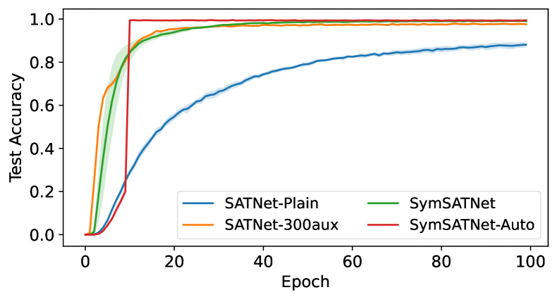
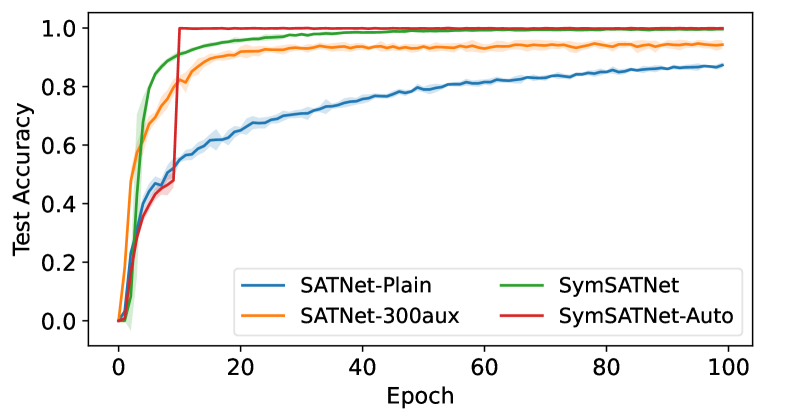
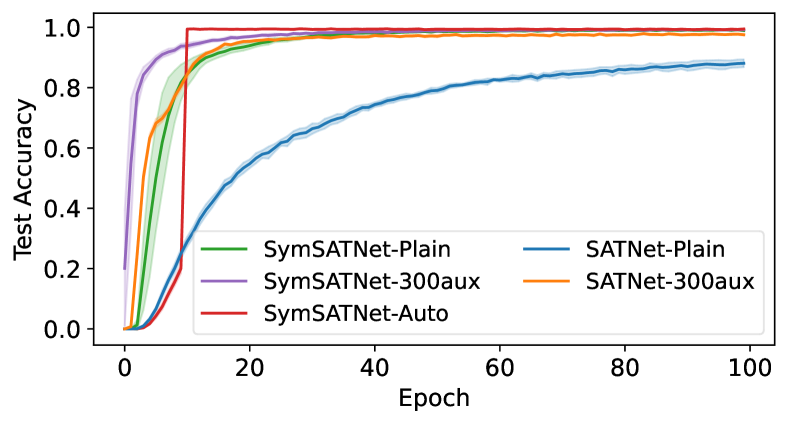
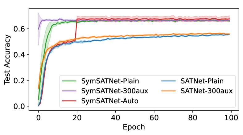
We used 9K training and 1K test examples generated by the Sudoku generator [Park, 2018]. Each example is a pair where the input assigns 31-42 cells (out of 81 cells) and the output specifies the remaining cells. SymSATNet was compared with SATNet-Plain without auxiliary variables, and SATNet-300aux with 300 auxiliary variables. We used binary cross entropy loss and Adam optimizer [Kingma and Ba, 2015], with the learning rate for SATNet-Plain and SATNet-300aux as the original work and for SymSATNet. We measured test accuracy, the rate of the correctly-solved Sudoku instances by the forward computations. We reported the average over 10 runs with confidence interval.
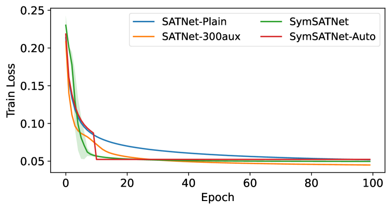
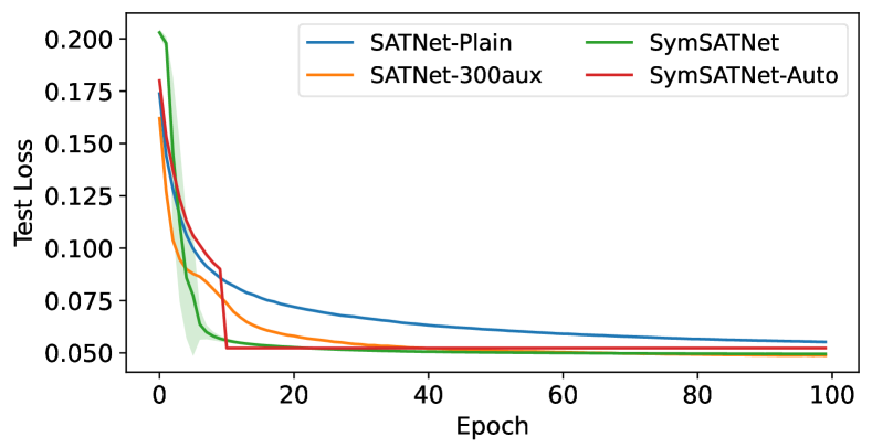
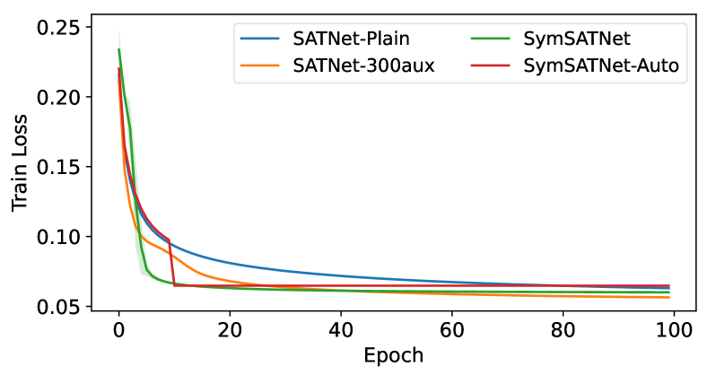
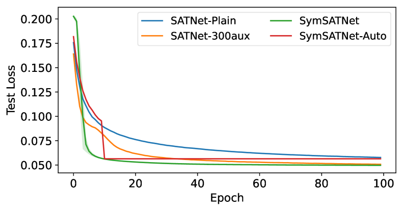
The results are in Figure 1 and Table 1. (SymSATNet-Auto refers to a variant of SymSATNet that uses SymFind as a subroutine to find symmetries automatically, and will be described later in this section.) Our SymSATNet outperformed SATNet-Plain and SATNet-300aux. On average, its 100 epochs finished - faster in terms of wall clock than two alternatives. due to the reduced number of iterations and avoidance of matrix operations. See Appendix G for the efficiency of SymSATNet. Despite the speed up, the best test accuracy of SymSATNet () was significantly better than SATNet-Plain () and slightly better than SATNet-300aux ().
| Model | Sudoku | Cube | ||
| Acc. | Time | Acc. | Time | |
| SATNet-Plain | 88.1% | 48.0 | 55.7% | 1.8 |
| 1.8% | 0.17 | 0.7% | 0.01 | |
| SATNet-300aux | 97.9% | 90.3 | 56.5% | 14.0 |
| 0.3% | 0.68 | 0.9% | 0.12 | |
| SymSATNet | 99.2% | 25.6 | 66.9% | 1.1 |
| 0.2% | 0.14 | 1.2% | 0.00 | |
| SymSATNet-Auto | 99.5% | 22.7 | 68.1% | 3.4 |
| 0.2% | 0.14 0.35 | 2.8% | 0.66 0.19 | |
Completion problem of Rubik’s cube
The Rubik’s cube is composed of faces, each of which has facelets. We considered a constraint satisfaction problem where we are asked to complete the missing facelets of the Rubik’s cube such that the resulting cube is solvable; by moving the cube, we can make all facelets in each face have the same colour, and no same colours appear in two faces. Let be a colour assignment of Rubik’s cube where the -th entry has if and only if the -th facelet of the -th face has colour . We formulate the optimisation objective of SATNet for Rubik’s cube using the relaxation of to for .
This problem has symmetries formalised by on . Here and are permutation groups on and , each of which captures the allowed moves of facelets, and the rotations of the whole cube. If a colour assignment is solvable, so is the transformation of by any permutations in . See Appendix F for more information about the symmetries of this problem.
We generated a basis in three steps. We first created and using the generators of each group [Finzi et al., 2021]. Next, we combined them using Theorem 2.3 to get , which was converted to a symmetric orthogonal basis via Gram-Schmidt. The final result has basis elements.
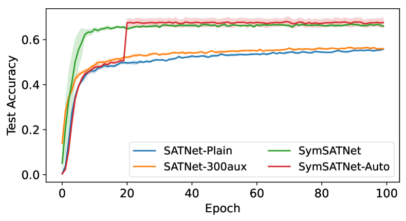
We used a dataset of 9K training and 1K test examples generated by randomly applying moves to the solution of the cube. Each example is a pair where assigns colours to facelets except for two corner facelets, two edge facelets, and one center facelet, and specifies the colours of those five missing facelets. In the test examples, only is used. We trained SymSATNet, SATNet-Plain, and SATNet-300aux for 100 epochs, under the same configuration as in the Sudoku case.
The results appear in Figure 1 and Table 1. On average, the -epoch training of SymSATNet completed faster in the wall-clock time than those of SATNet-Plain and SATNet-300aux. Also, it achieved better test accuracies () than these alternatives ( and ). Note that unlike Sudoku, the test accuracy of SATNet-300aux was only marginally better than that of SATNet-Plain, which indicates that both suffered from the overfitting issue. Note also the sharp increase in the training time of SATNet-300aux. These two indicate that adding auxiliary variables is not so effective for the completion problem for Rubik’s cube, while exploiting symmetries is still useful.
Automatic discovery of symmetries
To test the effectiveness of SymFind, we tested whether SymFind could find proper symmetries in Sudoku and Rubik’s cube. We applied SymFind to the parameter of SATNet-Plain in -th training epoch, where for Sudoku and for Rubik’s cube. For Sudoku, SymFind always recovered the full symmetries with in our 10 trials. For Rubik’s cube, the group of full symmetries is for . SymFind recovered all the parts except . Instead of this, the algorithm found or , or in our 10 trials. We manually observed that the entries of in the corresponding part were difficult to be clustered, violating the assumption of SymFind. This illustrates the fundamental limitation of SymFind.
To account for the limitation of SymFind, we refined the group of detected symmetries to a subgroup in an additional validation step, before training SymSATNet with those symmetries. In the validation step, we checked the usefulness of each part of the expression of in our grammar. Concretely, we rewrote only with the part in concern, where all the other parts of were masked by the trivial groups . After projecting with the masked groups using Reynolds operator, we measured the improvement of accuracy of SATNet over validation examples. Finally, we assembled only the parts that led to sufficient improvement. For example, if is discovered by SymFind, we consider the parts , , and . Then, we construct three masked groups , , and , and measure the accuracy of SATNet with projected by each over validation examples. If and show accuracy improvements greater than a threshold, we combine and to form , which is then used to train SymSATNet.
We used 8K training, 1K validation, and 1K test examples to train SymSATNet with symmetries found by SymFind and the validation step. We denote these runs by SymSATNet-Auto. We took a group discovered by SymFind in -th training epoch (with the same above) and constructed its subgroup via the validation step. SymSATNet was then trained after being initialised by the projection of with . The other configurations are the same as before.
As shown in Figure 1 and Table 1, SymSATNet-Auto performed the best for Sudoku () and Rubik’s cube () better than even SymSATNet. During the 10 trials with Sudoku, SymSATNet-Auto was always given the full symmetries in Sudoku. For Rubik’s cube, when SymSATNet-Auto was given correct subgroups (e.g., , ), then it performed even better than SymSATNet. In two of the 10 trials, slightly incorrect symmetries were exploited, but it outperformed SATNet-Plain and SATNet-300aux. These results show the partial symmetries of subgroups derived by the validation step are still useful, even when they are slightly inaccurate.
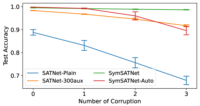
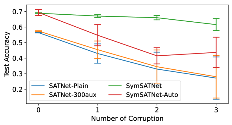
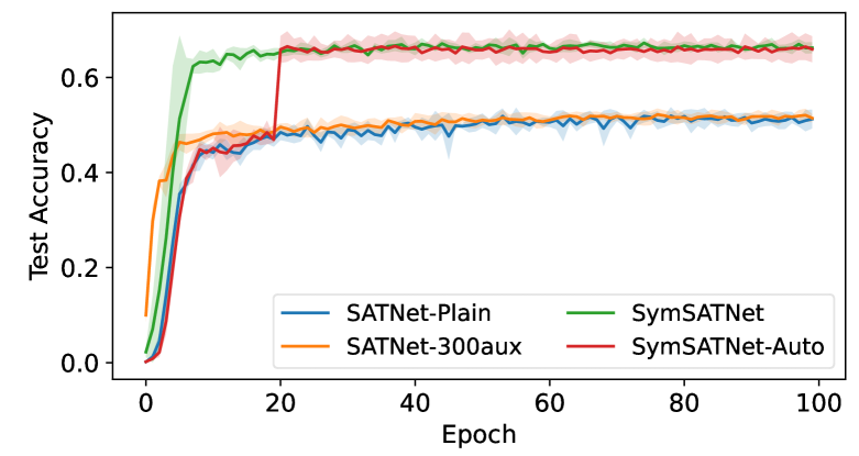
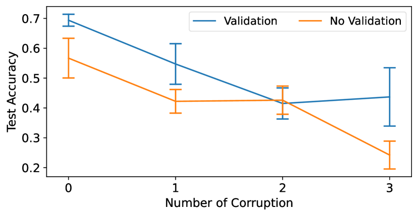
Robustness to noise
We tested robustness of SymSATNet and SymSATNet-Auto to noise by noise-corrupted datasets. We generated noisy Sudoku and Rubik’s cube datasets where each training example is corrupted with noise; it alters the value of a random cell or the colour of a random facelet to a random value other than the original. We used noisy datasets with 0-3 corrupted instances to measure the test accuracy, and tried 10 runs for each dataset to report the average and confidence interval. All the other setups are the same as before. Figure 2 shows the results. In both problems, SymSATNet was the most robust, showing remarkably consistent accuracies. SymSATNet-Auto showed comparable robustness to SATNet-300aux in noisy Sudoku, but outperformed the two baselines in noisy Rubik’s cube.
Next, to show the robustness of SymFind, we applied it to restore permutation groups from noise-corrupted -equivariant symmetric matrices . We picked for where , , are random permutations on , , , and is the identity permutation on , and
Then, we generated -equivariant symmetric matrices by projecting random matrices with standard normal entries into the space . Then, Gaussian noises from for are added to ’s entries, and the resulting matrix is given to SymFind.
| Group | Full Acc. | Partial Acc. |
| 76.6% | 79.2% | |
| 60.3% | 79.9% | |
| 77.5% | 87.0% | |
| 93.5% | 94.3% |
For each , we repeatedly generated and ran SymFind on for 1K times, and measured the portion where SymFind recovered exactly (full accuracy), and also the portion of cases where SymFind returned a subgroup of which is not the trivial group (partial accuracy). As Table 2 shows, the measured full accuracies were in the range of , and the partial accuracies were in the range of . These results show the ability of SymFind to recover meaningful and sometimes full symmetries.
Transfer learning
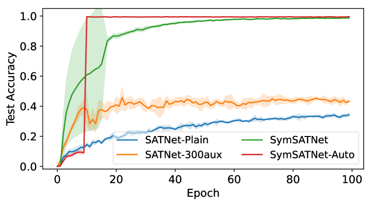
To test the transferability of SymSATNet, we generated Sudoku and Rubik’s cube datasets with varying difficulties, where each dataset consisted of 9K training and 1K test examples. For SymSATNet-Auto, we split the 9K training examples into 8K training and 1K validation examples. We used three levels of difficulties for Sudoku and Rubik’s cube (easy, normal, hard), based on the number of missing cells for Sudoku or missing facelets for Rubik’s cube. The input part of Sudoku examples was generated with 21 (easy), or 31 (normal), or 41 masked cells (hard), and the input part of Rubik’s cube examples was generated with 3 (easy), or 4 (normal), or 5 missing facelets (hard). For both problems, we used the training examples of easy or normal datasets for training, and the test examples of hard datasets for testing. We repeated every task in this experiment five times. Here we report the average test accuracies and confidence interval.
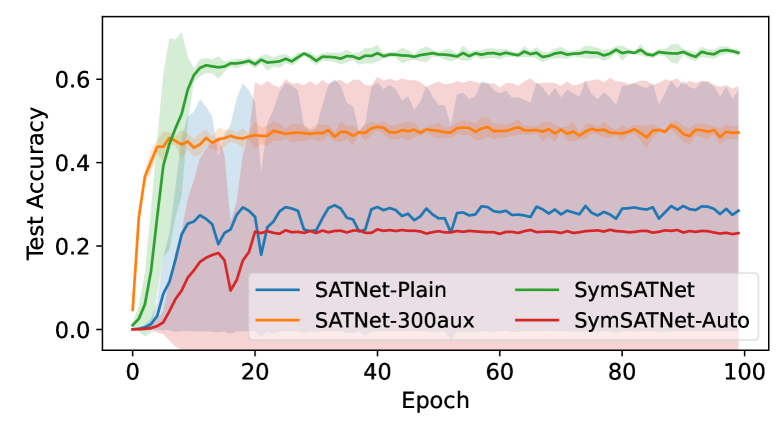
Figure 3 shows test accuracies throughout 100 epochs in the four types of transfer learning tasks. SymSATNet achieved the best result in the whole tasks; it succeeded in solving hard problems after learning from easier examples. As Figures 3(a) and 3(c) indicate, SymSATNet-Auto exploited the full group symmetries in Sudoku. For Rubik’s cube, Figure 3(b) shows SymSATNet-Auto achieved better performance over the baselines by finding partial symmetries. These results show the promise of SymSATNet and SymSATNet-Auto to learn transferable rules even from easier examples.
Note that for the easy Rubik’s cube dataset, SymSATNet-Auto showed poor performance (Figure 3(d)). The poor performance comes from the violation of the assumption of SymFind; the group symmetries sometimes did not emerge in SATNet in this case. In three out of five trials with the easy Rubik’s cube dataset, SATNet learnt nothing while producing the test accuracy, and SymFind returned the trivial group which equated SymSATNet-Auto with SATNet-Plain. In the remaining two trials, SATNet learnt correct rules, and SymFind and the validation step found correct partial symmetries, which led to the improved performance. These results exhibit the fundamental limitation of SymSATNet-Auto, whose performance strongly depends on the original SATNet.
6 Conclusion
We presented SymSATNet, that is capable of exploiting symmetries of the rules or constraints to be learnt by SATNet. We also described the SymFind algorithm for automatically discovering symmetries from the parameter of the original SATNet at a fixed training epoch, which is based on our empirical observation that symmetries emerge during training as duplicated or similar entries of . Our experimental evaluations with two rule-learning problems related to Sudoku and Rubik’s cube show the benefit of SymSATNet and the promise and limitation of SymFind. Although components of SymFind are motivated by the theoretical analysis of the space of equivariant matrices, such as Theorem 2.2, SymFind lacks a theoretical justification on its overall performance. One interesting future direction is to fill in this gap by identifying when symmetries emerge during the training of SATNet and proving probabilistic guarantees on when SymFind returns correct group symmetries.
Acknowledgements
This work was supported by the Engineering Research Center Program through the National Research Foundation of Korea (NRF) funded by the Korean Government MSIT (NRF-2018R1A5A1059921) and also by the Institute for Basic Science (IBS-R029-C1).
References
- Aloul et al. [2003] Fadi A Aloul, Arathi Ramani, Igor L Markov, and Karem A Sakallah. Solving difficult instances of boolean satisfiability in the presence of symmetry. IEEE Transactions on Computer-Aided Design of Integrated Circuits and Systems, 22(9):1117–1137, 2003.
- Aloul et al. [2006] Fadi A Aloul, Karem A Sakallah, and Igor L Markov. Efficient symmetry breaking for boolean satisfiability. IEEE Transactions on Computers, 55(5):549–558, 2006.
- Basu et al. [2021] Sourya Basu, Akshayaa Magesh, Harshit Yadav, and Lav R Varshney. Group equivariant neural architecture search via group decomposition and reinforcement learning. arXiv e-prints, pages arXiv–2104, 2021.
- Benhamou et al. [2010] Belaıd Benhamou, Tarek Nabhani, Richard Ostrowski, and Mohamed Réda Saıdi. Dynamic symmetry breaking in the satisfiability problem. In Proceedings of the 16th international conference on Logic for Programming, Artificial intelligence, and Reasoning. LPAR-16, Dakar, Senegal (April 25-may 1, 2010), 2010.
- Cingillioglu and Russo [2019] Nuri Cingillioglu and Alessandra Russo. Deeplogic: Towards end-to-end differentiable logical reasoning. In Proceedings of the AAAI 2019 Spring Symposium on Combining Machine Learning with Knowledge Engineering (AAAI-MAKE 2019), 2019.
- Cohen and Welling [2016] Taco S. Cohen and Max Welling. Group equivariant convolutional networks. In Proceedings of ICML’16, pages 2990–2999, 2016.
- Crawford [1992] James Crawford. A theoretical analysis of reasoning by symmetry in first-order logic. In AAAI Workshop on Tractable Reasoning, pages 17–22. Citeseer, 1992.
- Crawford et al. [1996] James M. Crawford, Matthew L. Ginsberg, Eugene M. Luks, and Amitabha Roy. Symmetry-breaking predicates for search problems. In Proceedings of the Fifth International Conference on Principles of Knowledge Representation and Reasoning, pages 148–159. Morgan Kaufmann Publishers Inc., 1996.
- Darga et al. [2004] Paul T. Darga, Mark H. Liffiton, Karem A. Sakallah, and Igor L. Markov. Exploiting structure in symmetry detection for CNF. In Proceedings of the 41st Annual Design Automation Conference, pages 530–534. Association for Computing Machinery, 2004.
- Darga et al. [2008] Paul T Darga, Karem A Sakallah, and Igor L Markov. Faster symmetry discovery using sparsity of symmetries. In 2008 45th ACM/IEEE Design Automation Conference, pages 149–154. IEEE, 2008.
- Dehmamy et al. [2021] Nima Dehmamy, Robin Walters, Yanchen Liu, Dashun Wang, and Rose Yu. Automatic symmetry discovery with Lie algebra convolutional network. Advances in Neural Information Processing Systems, 34, 2021.
- Devriendt et al. [2017] Jo Devriendt, Bart Bogaerts, and Maurice Bruynooghe. Symmetric explanation learning: Effective dynamic symmetry handling for SAT. In International Conference on Theory and Applications of Satisfiability Testing, pages 83–100. Springer, 2017.
- Dummit and Foote [1991] David S Dummit and Richard M Foote. Abstract algebra, volume 1999. Prentice Hall Englewood Cliffs, NJ, 1991.
- Evans and Grefenstette [2018] Richard Evans and Edward Grefenstette. Learning explanatory rules from noisy data. J. Artif. Intell. Res., 61:1–64, 2018.
- Finzi et al. [2021] Marc Finzi, Max Welling, and Andrew Gordon Wilson. A practical method for constructing equivariant multilayer perceptrons for arbitrary matrix groups. In Proceedings of ICML’21, pages 3318–3328, 2021.
- Kingma and Ba [2015] Diederik P. Kingma and Jimmy Ba. Adam: A method for stochastic optimization. CoRR, abs/1412.6980, 2015.
- Majumdar et al. [2012] Subrata Majumdar, Kalyan Kumar Dey, and Mohd Altab Hossain. Direct product and wreath product of transformation semigroups. GANIT: Journal of Bangladesh Mathematical Society, 31:1–7, Apr. 2012.
- Maron et al. [2019] Haggai Maron, Heli Ben-Hamu, Nadav Shamir, and Yaron Lipman. Invariant and equivariant graph networks. In Proceedings of ICLR’19, 2019.
- McKay [1976] Brendan D. McKay. Backtrack programming and the graph isomorphism problem. 1976.
- McKay [1981] Brendan D. McKay. Practical graph isomorphism. Congressus Numerantium, 30:45–87, 1981.
- Park [2018] Kyubyong Park. Can convolutional neural networks crack sudoku puzzles? https://github.com/Kyubyong/sudoku, 2018.
- Selsam et al. [2019] Daniel Selsam, Matthew Lamm, Benedikt Bünz, Percy Liang, Leonardo de Moura, and David L. Dill. Learning a SAT solver from single-bit supervision. In International Conference on Learning Representations, 2019.
- Topan et al. [2021] Sever Topan, David Rolnick, and Xujie Si. Techniques for symbol grounding with SATNet. In Advances in Neural Information Processing Systems, volume 34, pages 20733–20744. Curran Associates, Inc., 2021.
- Van Loan and Pitsianis [1993] Charles F Van Loan and Nikos Pitsianis. Approximation with kronecker products. In Linear algebra for large scale and real-time applications, pages 293–314. Springer, 1993.
- Wang et al. [2018] Po-Wei Wang, Wei-Cheng Chang, and J. Zico Kolter. The mixing method: low-rank coordinate descent for semidefinite programming with diagonal constraints. CoRR, abs/1706.00476, 2018.
- Wang et al. [2019] Po-Wei Wang, Priya L. Donti, Bryan Wilder, and J. Zico Kolter. Satnet: Bridging deep learning and logical reasoning using a differentiable satisfiability solver. In Proceedings of ICML’19, pages 6545–6554, 2019. URL https://github.com/locuslab/SATNet.git.
- Wang et al. [2020] Renhao Wang, Marjan Albooyeh, and Siamak Ravanbakhsh. Equivariant networks for hierarchical structures. In Proceedings of NeurIPS’20, pages 13806–13817, 2020.
- Yang et al. [2017] Fan Yang, Zhilin Yang, and William W. Cohen. Differentiable learning of logical rules for knowledge base reasoning. In Proceedings of NeurIPS’17, pages 2319–2328, 2017.
Appendix A Notation
For natural numbers and with , we write for the set . For an matrix , , and , we define by a matrix :
Also, if is a subgroup of , we denote it by .
Appendix B Proof of Theorem 2.3
In this section, we prove Theorem 2.3. Here we prove the direct sum, direct product, and wreath product cases by an argument similar to the previous work [Wang et al., 2020]. For the wreath product case, we slightly generalise the previous results [Wang et al., 2020], which considered only transitive group actions. We will use the notation from Theorem 2.3. Let and be permutation groups over and , respectively. Also, let , , , and .
Claim B.1.
The matrices , , , and are -equivariant. Also, the matrices of these types for all possible choices of , , , and form a linearly independent set.
Proof.
Pick arbitrary group elements and . Let and be the permutation matrices corresponding to and , respectively.
We prove the claimed equivariance below:
The third and fourth lines use the fact that and are invariant under the left or right multiplication of the permutation matrix . This holds because the orbits of are preserved by any permutation in , and those of are preserved by all permutations in , so that
| (6) |
Next, we show the claimed linear independence by analysing the indices of the nonzero entries of the four types of matrices in the claim.
-
1.
The matrices of the type for some are linearly independent, since their parts are linearly independent.
-
2.
The matrices of the type for some are also linearly independent by similar reason.
-
3.
Different matrices of the type for some and do not share an index of a nonzero entry, since different orbits of a group are disjoint. Thus, the matrices of this type are linearly independent.
-
4.
Different matrices of the type for some and do not share an index of a nonzeron entry. Thus, the matrices of this form are linearly independent.
Also, any matrices of the above four types form a linearly independent set because those linear combinations do not share any indices of nonzero entries. From this and the above reasoning for each of the four types of matrices it follows that the matrices of those four types are linearly independent, as claimed. ∎
Claim B.2.
The matrix is -equivariant. Also, the matrices of this shape for all possible choices of and form a linearly independent set.
Proof.
Pick arbitrary group elements and . Let and be the permutation matrices corresponding to and , respectively. Then,
For linear independence, we can prove it using the fact . ∎
Claim B.3.
Recall and . The matrices such that for and are -equivariant. Also, the matrices of these types for all possible choices of , , , , and form a linearly independent set.
Proof.
Pick arbitrary group elements and . Let and be the permutation matrices corresponding to and for . We can express and by
Then, we prove the following equivariance:
| (7) | ||||
| (8) | ||||
| (9) | ||||
Here, (7) and (8) use the same argument in (6), and (9) uses the fact that for any and . For linear independence, we again use the fact to show the orthogonality of all possible matrices of types and . ∎
Claim B.4.
The number of basis elements of , , and can be computed as follows:
Proof.
First, we derive some general fact on a finite permutation group. Let be a permutation group on for some . Consider the action of on the space of -dimensional vectors by the row permutation action for any . Define . Consider the following linear operator
which can also be represented as the following matrix:
The operator is a projection map, since
Also, we have where is the image of the function . Now, by noting that a linear projection map has only eigenvalues and , the dimension of can be computed by the sum of eigenvalues of , i.e., . Also, using Burnside’s lemma, we can count the orbits of (acting on ) by
Putting together, we get
| (10) |
Next, we instantiate what we have just shown above for the following case that is the following group:
for some permutation group on . Note that is a permutation group on . As explained above, can act on the space of -dimensional vectors . By vectorizing matrices, we can express the space of -equivariant linear maps on by
Thus, . We now calculate the dimension of using the relationship in (10):
| (11) |
Proof of Theorem 2.3
Claims B.1, B.2, and B.3 show that each set of matrices on the right-hand side of the equations in Theorem 2.3 consists of linearly independent matrices, and it is contained in the corresponding space of equivariant linear maps. Furthermore, Claim B.4 shows that the matrices in the set span the whole of the space of equivariant linear maps, since their number coincides with the dimension of the space. Hence, these three claims complete the proof of the theorem.
Appendix C Proofs of Theorem 3.2 and Lemma 3.3
Proof of Theorem 3.2
Assume that is -equivariant. Pick any . Then, preserves the standard action of on via its permutation matrix. Thus, , where denotes the permutation matrix . This equation is equivalent to
| (12) |
since . Using this equality, we show that the optimisation objective is invariant with respect to ’s action:
Here is the usual trace operator on matrices, the third equality uses the cyclic property of , and the last equality uses (12).
We move on to the proof of the converse. Assume and the equation (3) holds for every and . Pick any . Then, for all ,
The first equality follows from (3), and the second from our derivation above. But the space of matrices of the form is precisely that of symmetric positive semi-definite matrices, which is known to contain independent elements. Since is precisely the dimension of the space of symmetric matrices, the above equality for every implies that , that is, . This gives the -equivariance of , as desired.
Proof of Lemma 3.3
Pick arbitrary and . Let be the columns of in order, and be those of in order. Then, for every if and only if for all . The latter is equivalent to the statement that for every .
Appendix D Subroutines of SymFind
In this section, we describe the subroutines SumFind and ProdFind of our SymFind algorithm.
D.1 Detection of direct sum
We recall the distributivity law of group constructors [Dummit and Foote, 1991, Majumdar et al., 2012]:
By this law and the fact that for all , any permutation group definable in our grammar can be expressed as a direct sum
| (13) |
where each and is either or . Let
and be the natural number such that is a permutation group on . Since both and have only one orbit for all , each also has only one orbit. Hence, by Theorem 2.3,
where
This means that all off-diagonal blocks of any -equivariant matrices are constant matrices, just like the matrix shown in (b) of Figure 5.
Given a matrix , the subroutine SumFind aims at finding a permutation and the split for such that is approximately -equivariant for some permutation group on and this group has the form in (13) where is a permutation group on . The result of the subroutine is .


SumFind achieves its aim using two key observations. The first is an important implication of the -equivariance condition on that we mentioned above: when the split is used to group entries of into blocks, the -equivalence of implies that the off-diagonal blocks of are constant matrices. This implication suggests one approach: for every permutation on , construct the matrix , and find a split for some such that off-diagonal blocks of from this split are constant matrices. Note that this approach is not a feasible option in practice, though, since there are exponentially many permutations . The second observation suggests a way to overcome this exponential blow-up issue of the approach. It is that when is -equivariant, in many cases its diagonal blocks are cyclic in the sense that the -th entry of a block is the same as the -th entry of the block. This pattern can be used to search for a good permutation efficiently.
SumFind works as follows. It first finds a permutation and a split using the process that we will explain shortly. Figure 5 illustrates the input matrix , and its permuted that has nine blocks induced by the split of . Then, SumFind calls SymFind recursively on each diagonal block of and gets, for every ,
where . Finally, SumFind returns
where
We now explain the first part of SumFind that finds a permutation and a split . For simplicity, we ignore the issue of noise, and present a simpler version that uses equality instead of approximate equality (i.e., being close enough). We start by initialising , the identity permutation, and . Then, we pick an index from the set . Then, we locate in the -th entry by swapping the indices and , which can be done by updating
Here , , and for . Next, we find a new index which is suitable to swap with the index in the updated . As Figure 5 shows, we need to find such that , , and . Once we find such , we swap the indices and by updating
We repeat this process to find an index and the "L-shaped" entries which preserve the cyclic pattern. If we cannot find such , we stop the process, and check (i) whether all rows in are the same and also (ii) whether all columns in are the same. If the answers for both (i) and (ii) are yes, we move on to find the next diagonal block in in the same manner.
If (i) or (ii) has a negative answer, we go back to the step right before choosing from and resetting and to the values at that step. Then, we repeat the above process with a new choice of from . If no choice of leads to the situation where both (i) and (ii) have positive answers, then we conclude that , and move on to find the next diagonal block of starting from the index .
D.2 Detection of direct product
Let be a matrix. Assume that we are given with . If for some permutation groups and , the matrix lies in (i.e., is -equivariant), then can be represented as a linear combination of Kronecker products:
| (14) |
where , , and is a natural number.
The representation suggests the following strategy of finding a group of symmetries of that is the direct product of two permutation groups on and . First, we express as a linear combination of Kronecker products for and . Second, we pick a pair and in the linear combination. Third, we call SymFind recursively on and to get group-permutation pairs and . Finally, we return where
Our ProdFind is the implementation of the strategy just described. The only non-trivial steps of the strategy are the first two, namely, to find the representation of in (14), and to pick good and . ProdFind also has to account for the fact that the representation in (14) holds only approximately at best in our context.
For the representation finding, ProdFind uses the technique [Van Loan and Pitsianis, 1993] that solves the following optimisation problem for given :
| (15) |
The technique performs the singular value decomposition of the rearranged matrix of defined by
| (16) |
for and . To understand why it does so, note that the optimisation problem in (15) is equivalent to the following problem:
| (17) |
This new optimisation problem can be solved using SVD. Concretely, if we have the SVD of , namely,
| (18) |
where is the rank of , is the -th largest singular value, and and are the corresponding left and right singular vectors, we can solve the minimisation problem (17) by reshaping each term of (18) corresponding to the largest singular values, i.e.,
The first step of ProdFind is to apply the above technique [Van Loan and Pitsianis, 1993]. ProdFind performs the SVD of the matrix and gets in (18) where for some . Then, it sets , and picks so that all ’s with are included when we approximate .
The second step of ProdFind is to pick and . ProdFind simply picks and that correspond to matrices (reshaped from and ) for the largest singular value . We empirically observed that the matrices and are most informative about the symmetries of , and are least polluted by noise from the training of SATNet.
The third and fourth steps of ProdFind are precisely the last two steps of the strategy that we described above.
Our description of SymFind in the main text says that ProdFind gets called for all the divisors of with being , since we do not know the best divisior a priori, and that each invocation generates a new candidate in the candidate list . However, in practice, we ignore some divisors that violates our predefined criteria. In particular, we set an upper bound on , and use a divisor only when ProdFind for picks with , i.e., not too many terms are considered in the linear combination of Kronecker products. This criterion can be justified by the following lemma:
Lemma D.1.
Let be the direct product of permutation groups and on and , respectively. Consider a -equivariant matrix and its rearranged version in (16). Then, .
Proof.
Having fewer basis elements is generally better because it leads to a small number of parameters to learn in SymSATNet. The above lemma says that a divisor with large (which roughly corresponds to the large rank of in the lemma) leads to large and . Our criterion is designed to avoid such undesirable cases.
D.3 Detection of wreath product
Assume that the permutation groups and act transitively on and (i.e., for all and , there are and such that and ). We recall that in this case, every equivariant matrix under the wreath product of groups can be expressed as follows [Wang et al., 2020]:
| (21) |
for some and , where , are everywhere-one, identity matrices in . We use this general form of -equivariant matrices and make ProdFind detect the case that symmetries are captured by a wreath product.
Our change in ProdFind is based on a simple observation that the form in (21) is exactly the one in (14) with . We change ProdFind such that if we get while runnning , we check whether can be written as the form in (21). This checking is as follows. Using given and , we create blocks
of submatrices in for all . Then, we test whether all and for are constant matrices (i.e., matrices of the form for some ). If this test passes, has the desired form. In that case, we compute and from , and recursively call SymFind on and .
We can also make detect wreath product. The required change is to perform a similar test on each diagonal block of the final computed by . The only difference is that when the test fails, we look for a rearrangement of the rows and columns of the diagonal block that makes the test succeed. If the test on a diagonal block succeeds (after an appropriate rearrangement), the group corresponding to this block, which is one summand of a direct sum, becomes a wreath product.
Appendix E Computational Complexity of SymFind
In this section, we analyse the computational complexity of our SymFind algorithm in terms of the dimension of the input matrix. Suppose that an matrix is given to SymFind as an input. The complexity of SymFind shown in Algorithm 1 is for any arbitrarily small .
We can show the claimed complexity of SymFind using induction. When SumFind is called in the line 9 of Algorithm 1, it first spends time for clustering, and then makes recursive calls to SymFind with submatrices for . Each of these calls takes time by induction, and the total cost of all the calls is . Also, when ProdFind is called in the lines 11-12 of Algorithm 1, for each divisor of , ProdFind performs SVD in steps, and makes recursive calls to SymFind. The recursive calls here together cost by induction. Thus, the loop in lines 11-14 costs , where is the number of divisors of , since for any arbitrarily small . It remains to show that applying the Reynolds operator (in the lines 2 and 6) and counting the number of basis elements (in the line 15) take steps. The former costs since it is actually an average pooling operation when we consider permutation groups. The latter costs at most (when it is given ).
Appendix F Symmetries in Sudoku and Rubik’s Cube Problems
In this section, we describe the group symmetries in Sudoku and the completion problem of Rubik’s cube. In both problems, we can find certain group acting on such that for any valid assignment of problem, is also valid for any .
In Sudoku, we denote the first three rows of a Sudoku board by the first band, and the next three rows by the second band, and the last three rows by the third band. In the same manner, we denote each three columns by a stack. For Sudoku problem, one can observe that any row permutations within each band preserve the validity of the solutions. Also, the permutations of bands preserve the validity. We can represent this type of hierarchical actions by wreath product groups. In this case, 3 bands are permuted in a higher level, and 3 rows in each band are permuted in a lower level, which corresponds to the group action of . The same process can be applied to the stacks and the columns, which also corresponds to the group . Furthermore, the permutations of number occurences in Sudoku (e.g., switching all the occurences of 3’s and 9’s) also preserves the validity of the solutions. In this case, any permutations over are allowed, thus represents this permutation action. Overall, we have three permutation groups, , , and . These three groups are in different levels; is at the outermost level, and is at the innermost level. Note that these three types of actions are commutative, i.e., the order does not matter if we apply the actions in different levels. This relation forms a direct product between each level, and we conclude .
For Rubik’s cube, we first introduce some of the conventional notations. We are given a Rubik’s cube composed of 6 faces and 9 facelets in each face. There are also 26 cubies in the Rubik’s cube, and they are classified into 8 corners, 12 edges, and 6 centers. To change the color state of Rubik’s cube, we can move the cubies with 9 types of rotations, which are denoted by , , , , , , , , . We can represent each color state of the Rubik’s cube by a function from to , where encodes the face and facelets, and encodes the colors. The initial state of Rubik’s cube is satisfying for all . If there exists a sequence of rotations that transforms to the initial state, then is solvable. Our completion problem of Rubik’s cube is to find a color assignment such that the assignment is solvable. For example, if a corner cubie contains 2 same colors, it is not solvable because these adjacent same colors cannot be separated by the 9 types of rotations.
We can observe the following group symmetries in the completion problem of Rubik’s cube: any solvable color state is still solvable after being transformed by the 9 types of rotations. These 9 rotations generate a permutation group acting on the facelets of a Rubik’s cube, which is called the Rubik’s cube group. Furthermore, like Sudoku, we can also consider the permutations of color occurences. In this case, if we assume the colors and are initially on the opposite sides, then the solvability can be broken by switching the colors and since the colors and are then no longer on the opposite sides. Considering this, computing all possible permutations acting on the color occurences is not trivial. Instead, we can generate such group by 3 elements, each of which corresponds to the rotation in one of the three axes in 3-dimension. Finally, these two groups and form different levels of actions, and actions from different levels commute each other. Therefore, we conclude .
Appendix G Efficient Implementation of SymSATNet
Our SymSATNet includes forward-pass and backward-pass algorithms as described in Section 3. Here, we describe slight changes of the forward-pass and backward-pass algorithms in SymSATNet, and the improvement of efficiency obtained by these changes. Algorithms 2 and 3 are the forward pass algorithms of SATNet and SymSATNet, and Algorithms 4 and 5 are the backward pass algorithms of SATNet and SymSATNet. In those algorithms, we let be the -th column of the matrix , and and be the previous -th columns of and before the update. Also, let , and be the n-dimensional one-hot vector whose only -th element is . Note that our algorithms are only slightly different from the ones of original SATNet, and the only difference is that the inner products are substituted by which can be directly derived from . This allows us to implement the forward-pass and the backward-pass algorithm of SymSATNet in the same manner as the original SATNet.
The above changes bring a small difference in the computational complexity. In SATNet, new matrices and are required for the rank- update in each loop. Recall that and imply . SATNet costs twice every iteration, in the lines 6, 8 of Algorithm 2 and in the lines 5, 7 of Algorithm 4. SymSATNet costs once every iteration, in the line 5 of Algorithm 3 and in the line 5 of Algorithm 5. Another slight difference is in the first line of the body of each for loop, where SATNet computes , but SymSATNet uses the constant . If we denote the required number of iterations by , then SATNet costs , and SymSATNet costs inside the loop. These make one of the major differences between the runtime of SATNet and SymSATNet, since these are scaled by , the number of iterations until convergence. Outside the loop, SATNet additionally costs in the line 3 of Algorithm 2, and SymSATNet costs in the forward computation of in (4), and in the backward computation with the chain rule in (5). These costs are not significant because each of these occurs only once every gradient update in SATNet and SymSATNet.
We also inspected the values of in SATNet and SymSATNet in a training run for Sudoku and Rubik’s cube problem in the configuration we used in our experiments. For Sudoku, SATNet repeated the loop times on average, in the range of , while SymSATNet finished the loop in on average, in the scope of . For Rubik’s cube, SATNet completes the loop in on average, whose scope was , while SymSATNet iterates times on average, with the range . These results show that the component is reduced in SymSATNet for those two problems, and bring further improvement of efficiency in practice.
Appendix H Hyperparameters
In this section, we specify the hyperparameters to run SymFind algorithm and the validation steps in SymSATNet-Auto. Each validation step requires a threshold of improvement of validation accuracy to measure the usefulness of each smaller part in a given group, i.e., only the smaller parts showing improvement greater than the threshold were considered to be useful, and were combined to construct the whole group. We determined this threshold by the number of corruption in the dataset; for the dataset with 0 and 1 corruption, for 2 corruption, and for 3 corruption. Also, our SymFind algorithm receives as an input, which determines the degree of sensitivity of SymFind. In practice, this tolerance was implemented by two hyperparameters, say and . was used to compute a threshold to decide whether a pair of entries have the same value within our tolerance so that they have to be clustered. We computed this threshold by the multiplication of and the norm of input matrix, and was fixed by for both problems. played a role of a threshold to conclude that the input matrix truly has the symmetries under the discovered group by SymFind. was used in the last step of SymFind, where the largest group is selected among the candidates. With the Reynolds operator, we computed the distance between the input matrix and the equivariant space under each candidate group, and filtered out the groups whose distance is greater than . We determined by the number of corruption in the dataset; for the dataset with 0 corruption, for 1 corruption, for 2 corruption, and for 3 corruption.
Appendix I GPU Usage
The implementation of SymSATNet is based on the original SATNet code, and thus the calculations in the forward-pass and the backward-pass algorithms of SymSATNet can be accelerated by GPU. We used GeForce RTX 2080 Ti for every running of SATNet and SymSATNet.
Appendix J Ablation Study of Validation Steps
In this section, we present the results of ablation study for the additional validation step in SymSATNet-Auto. All the configurations are the same, except that the discovered group symmetries by SymFind are directly exploited by SymSATNet without the subsequent validation step. We used noisy Sudoku and Rubik’s cube datasets, and repeated our experiment with each dataset ten times. Here we report the average test accuracies with confidence interval.
In Sudoku, our SymFind algorithm always succeeded in finding the full group symmetries, and these correct symmetries were preserved by the validation step since they always significantly improved the validation accuracies after projecting the parameter of SATNet. For this reason, omitting the validation step did not change the performance of SymSATNet-Auto. Thus, we do not plot the results for the Sudoku case. For Rubik’s cube, the results are shown in Figure 6. Without the validation step, SymSATNet-Auto often overfit into the wrong group symmetries induced by the noise in the parameter matrix of SATNet, resulting in lower improvement of performance. These results show that the additional validation step is useful not only when the training and the test examples share the same distribution, but also when the distribution of training examples is the perturbation of that of test examples by noise.
Appendix K Emergence of Symmetries in SATNet
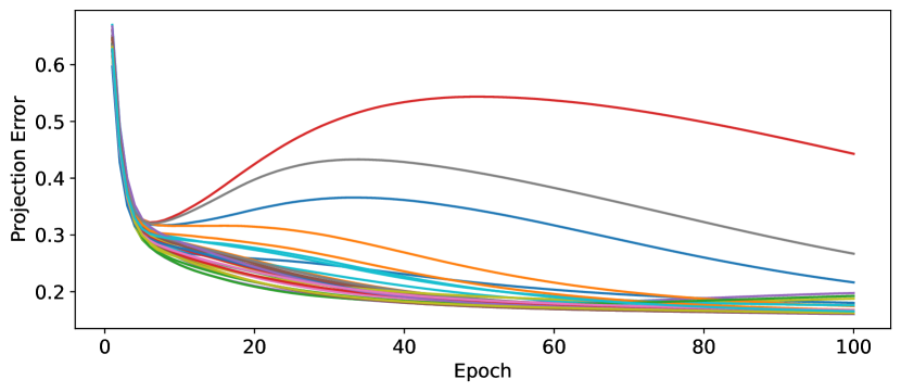
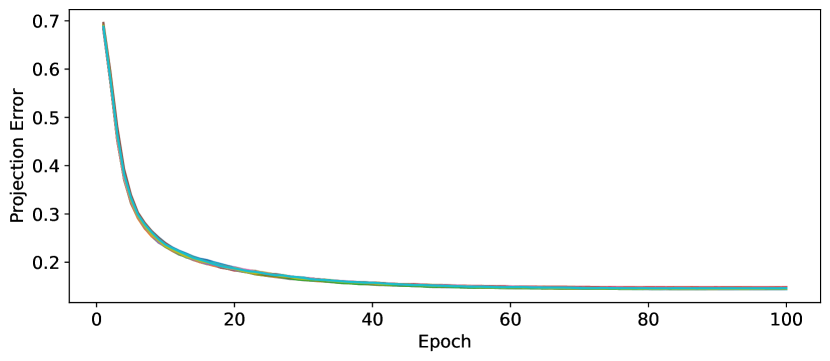
In this section, we report our experiment for detecting the appearance and disappearance of symmetries in the SATNet’s parameter matrix throughout the training epochs. We measured how close is to , the space of equivariant matrices under , by computing (denoted by projection error below) where is the ground-truth permutation group for a given learning problem (e.g., Sudoku or Rubik’s cube). We evaluated the projection errors throughout 100 training epochs. Our experiment for each problem was repeated 30 times.
Figure 7 shows the results. For Sudoku, in multiple cases out of 30 trials, the projection error hit the lowest point around the 5-10th epochs, and after these epochs, the projection error started to increase until certain epochs, so that the training ended with a high projection error. We did not observe any clear difference in the training loss (or the test loss) between these cases with high projection errors and the other cases (which showed low projection errors). This result suggests possible overfitting from the perspective of symmetry discovery in the original SATNet. For Rubik’s cube, in all of our trials, the projection error always decreased throughout the epochs, and no sign of overfitting was detected. Answering why this is the case is an interesting topic for future research. Also, in the very beginning of the training for both problems, the projection errors were not sufficiently small. By choosing proper stopping epochs in SymSATNet-Auto, we can avoid high projection errors, as we did (i.e., we picked the 10th epoch for Sudoku, and the 20th epoch for Rubik’s cube). Finally, we point out that there may be factors other than the projection error that influence the performance of our symmetry-discovery algorithm. If found, those factors would become useful tools for analysing the theoretical guarantees of SymFind algorithm, and we leave it to future work.
Appendix L SymSATNet with Auxiliary Variables
| Model | Sudoku | Cube | ||||
| Train Acc. | Test Acc. | Time | Train Acc. | Test Acc. | Time | |
| SATNet-Plain | 93.5% | 88.1% | 48.0 | 99.4% | 55.7% | 1.8 |
| 1.2% | 1.3% | 0.17 | 0.1% | 0.5% | 0.01 | |
| SATNet-300aux | 99.8% | 97.9% | 90.3 | 99.8% | 56.5% | 14.0 |
| 0.0% | 0.2% | 0.68 | 0.0% | 0.6% | 0.12 | |
| SymSATNet-Plain | 98.8% | 99.2% | 25.6 | 67.1% | 66.9% | 1.1 |
| 0.1% | 0.2% | 0.14 | 0.2% | 0.9% | 0.00 | |
| SymSATNet-300aux | 99.2% | 99.3% | 53.6 | 69.6% | 67.6% | 9.5 |
| 0.1% | 0.1% | 0.56 | 0.4% | 0.5% | 0.29 | |
| SymSATNet-Auto | 99.3% | 99.5% | 22.7 | 70.2% | 68.1% | 3.4 |
| 0.1% | 0.2% | 0.14 0.35 | 3.1% | 2.0% | 0.66 0.19 | |
By introducing auxiliary variables, the original SATNet can achieve higher expressive power and better performance while trading-off the runtime efficiency. The similar process can be done in SymSATNet. If a permutation group captures group symmetries of a problem to be solved without auxiliary variables, then represents the extension of the same symmetries with the auxiliary variables. The singleton group here acts trivially (i.e., permutes nothing) on those auxiliary variables.
We now report the findings of our experiments with SymSATNet with 300 auxiliary variables (SymSATNet-300aux) that retains the above extension of group symmetries. We compared the performance of SymSATNet-300aux with the other four models that we used before, on the 0-corrupted Sudoku and Rubik’s cube datasets. We denote SymSATNet without auxiliary variables by SymSATNet-Plain to distinguish it from SymSATNet-300aux. We repeated the training for each dataset 10 times. Here we report the average and best test accuracies, the average training times, and confidence interval. We trained SymSATNet-300aux with the learning rate , which is the same as SymSATNet-Plain. All the experimental setups were the same as before.
Figure 8 and Table 3 show the results. In both tasks, SymSATNet-300aux outperformed all the other models except SymSATNet-Auto. Also, for Rubik’s cube, SymSATNet-300aux showed the fastest convergence in epoch among all the models. Note that both the test accuracies and the training times of SymSATNet-300aux were remarkably improved over those of SATNet baselines. These results demonstrate that SATNet with auxiliary variables still enjoyed the benefits by exploiting a minor extension of group symmetries, although the benefits were not as significant as in the case of SymSATNet-Plain.
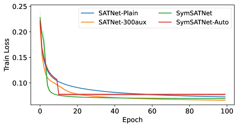
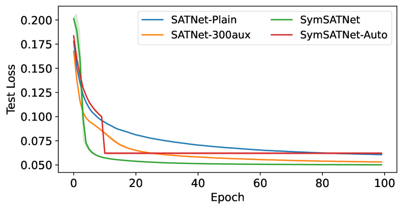
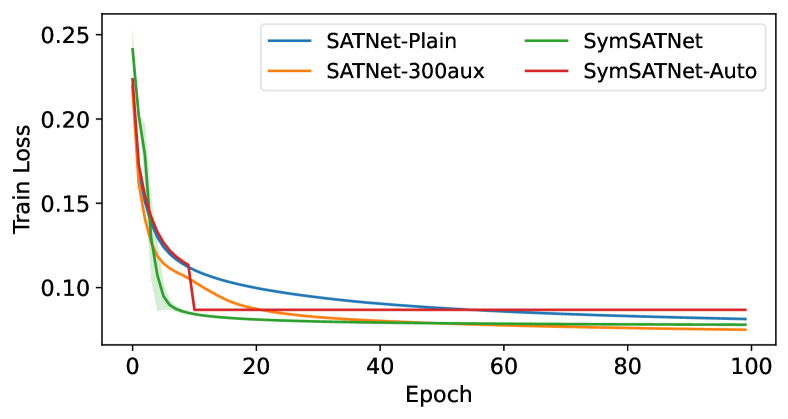
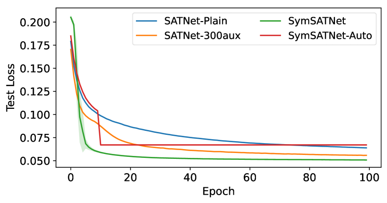
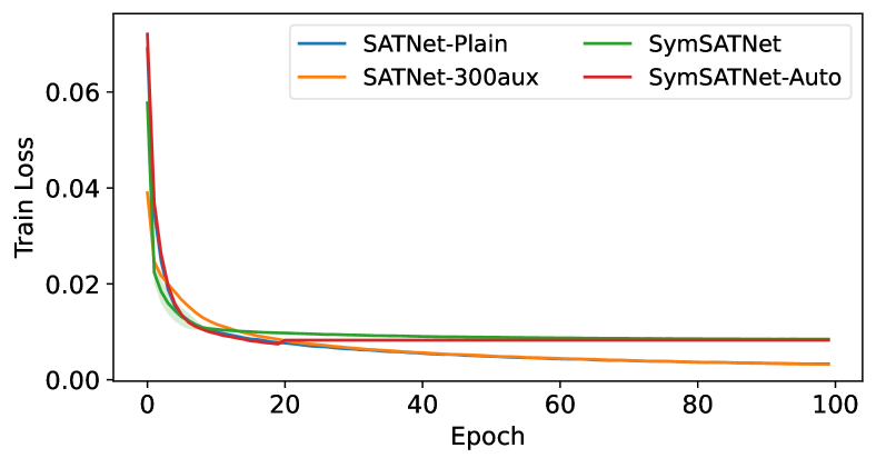
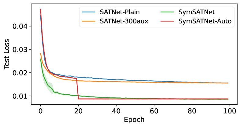
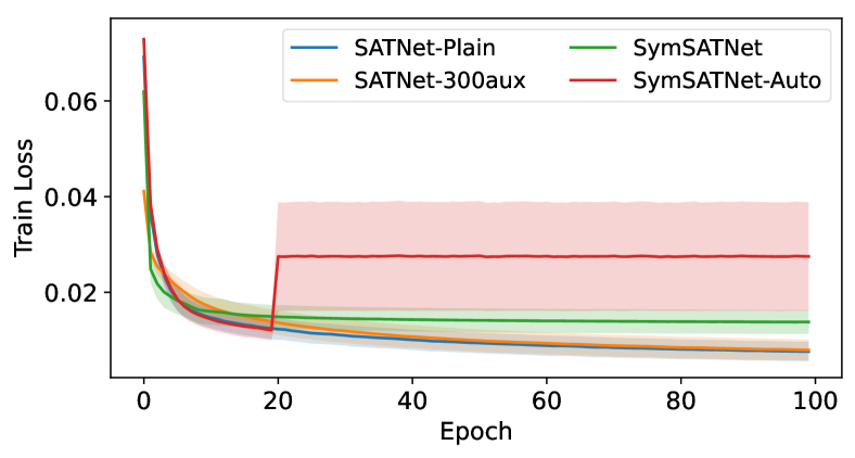
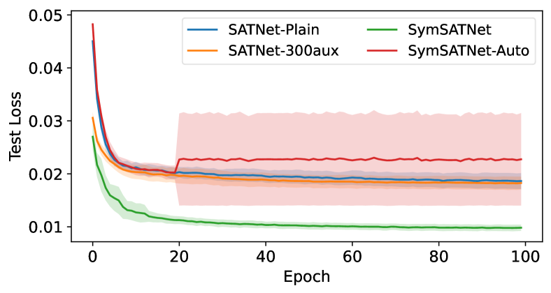
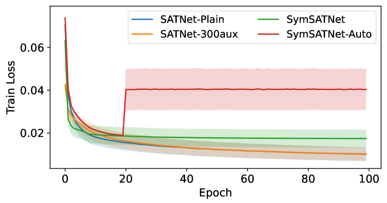
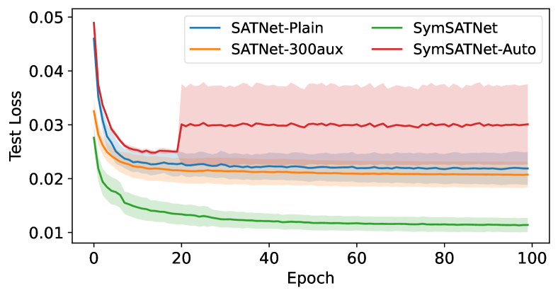
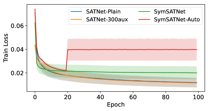
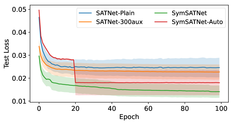
Appendix M Loss Curves