Young, blue, and isolated stellar systems in the Virgo Cluster
I. 2-D Optical spectroscopy

Abstract

We use panoramic optical spectroscopy obtained with MUSE@VLT to investigate the nature of five candidate extremely isolated low-mass star forming regions (Blue Candidates, BCs hereafter) toward the Virgo cluster of galaxies. Four of the five (BC1, BC3, BC4, BC5) are found to host several H ii regions and to have radial velocities fully compatible with being part of the Virgo cluster. All the confirmed candidates have mean metallicity significantly in excess of that expected from their stellar mass, indicating that they originated from gas stripped from larger galaxies. In summary, these four candidates share the properties of the prototype system SECCO 1, suggesting the possible emergence of a new class of stellar systems, intimately linked to the complex duty cycle of gas within clusters of galaxies. A thorough discussion on the nature and evolution of these objects is presented in a companion paper, where the results obtained here from MUSE data are complemented with Hubble Space Telescope (optical) and Very Large Array (Hi) observations.

1 Introduction

The publication of catalogues of compact Hi sources from the ALFALFA (Adams et al., 2013) and GALFA (Saul et al., 2012) surveys triggered observational campaigns aimed at detecting their stellar counterparts, in search of new very dark local dwarf galaxies hypothesised to be associated with the gas clouds (Sand et al., 2015; Bellazzini et al., 2015a; Tollerud et al., 2015). The new experiments failed to find a significant population of such objects (see, e.g., Beccari et al., 2016), still a few new interesting stellar systems were identified (see, e.g., Giovanelli et al., 2013; McQuinn et al., 2015; Tollerud et al., 2015; Cannon et al., 2015; Bennet et al., 2022).

One of the most curious cases is SECCO 1 (also known as AGC 226067; Bellazzini et al., 2015a, b; Sand et al., 2015; Adams et al., 2015), a low-mass ($M_{\star}\simeq 10^{5}~{}M_{\odot}$, $M_{HI}\simeq 2\times 10^{7}~{}M_{\odot}$) star-forming stellar system lying within the Virgo cluster of galaxies. Given the very low stellar mass, the high mean metallicity ($\langle 12+{\rm log}(O/H)\rangle=8.38\pm 0.11$) implies that the gas fuelling star formation in SECCO 1 was stripped from a relatively massive gas-rich galaxy (Beccari et al., 2017; Sand et al., 2017; Bellazzini et al., 2018), either by a tidal interaction or by ram pressure exerted by the hot intra cluster medium (ICM). Indeed, star formation is known to occur in gas clouds stripped from galaxies via both channels (see, e.g., Pasha et al., 2021; Poggianti et al., 2019, and references therein). However, in both cases, the star-forming stripped knots are always seen in proximity to the parent galaxy and/or connected to the parent galaxy either by tidal tails or by the jellyfish structures that are the classical fingerprint of ram-pressure stripping (see, e.g., Gerhard et al., 2002; Yoshida et al., 2012; Fumagalli et al., 2011, 2014; Kenney et al., 2014; Fossati et al., 2016; Bellazzini et al., 2019; Nidever et al., 2019; Corbelli et al., 2021a, b). In contrast, SECCO 1 is extremely isolated, lying more than 200 kpc, in projection, from the nearest candidate parent galaxy (Sand et al., 2017; Bellazzini et al., 2018; Jones et al., 2022a).

Simple theoretical arguments (Burkhart & Loeb, 2016) as well as dedicated hydrodynamical simulations (Bellazzini et al., 2018; Calura et al., 2020), suggest that gas clouds similar to SECCO 1 may survive as long as $\sim 1$ Gyr within clusters of galaxies, kept together by the pressure confinement of the ICM, thus leaving room for very long voyages from the site of origin. Star formation is also expected to occur in the meanwhile (Calura et al., 2020; Kapferer et al., 2009). If cloudlets such as these are indeed able to survive such long times and form stars, a rich population of them should be among the inhabitants of galaxy clusters, given the complex processes in which the gas is involved in these environments (Poggianti et al., 2019; Boselli et al., 2021).

Prompted by these considerations, a search for similar systems in the Virgo cluster was performed (see Sand et al., 2017; Jones et al., 2022b) and a sample of five Blue Candidates (BCs) were selected from UV and optical images, as described in Jones et al. (2022a). To confirm the nature of these BCs, spectroscopic follow-up is essential to a) measure their radial velocity and confirm their location within the Virgo Cluster; b) quantify any ongoing star formation by detecting and analyzing associated H ii   regions, and c) estimate the metallicity of the gas in star forming regions, a crucial diagnostic for assessing the origin of these systems.

Here we present the results of VLT@MUSE (Bacon et al., 2014) observations of five such blue candidate stellar systems, fully analogous to the study by Beccari et al. (2017, Be17 hereafter) for SECCO 1. Four of them are confirmed as likely residing in Virgo and similar to SECCO 1. Individual H ii regions are identified, velocities and line fluxes are measured from their spectra and metallicity estimates are provided. Finally, their chemical and kinematic properties are briefly discussed. In a companion paper (paper II; Jones et al., 2022a, Pap-II hereafter), Hubble Space Telescope (HST) imaging and photometry as well as new Very Large Array (VLA) and Green Bank telescope (GBT) Hi observations for the BCs are presented. The companion paper also discusses the nature and origin of this potentially new class of stellar systems, based on the entire set of available observations. A more detailed discussion on BC3, also known as AGC 226178, the only system that has been subject of previous analyses (Cannon et al., 2015; Junais et al., 2021), has been presented by Jones et al. (2022b).

Figure 1: Maps of the H$\alpha$ emission from BC1 (a) and BC3 (b). The levels of the contours are at 2, 4, 8, 16, 32, 64, 128, 256 $\times 10^{-20}$ erg cm ^-2 s^-1. Right ascension and declination are in degrees.

Figure 2: Maps of the H$\alpha$ emission from BC4L (a), BC4R (b), and BC5 (c). The levels of the contours are at 2, 4, 8, 16, 32, 64, 128, 256 $\times 10^{-20}$ erg cm ^-2 s^-1. Right ascension and declination are in degrees.

2 Observations and data reduction

Integral field unit optical (4650-9300$\;\buildrel\circ\over{\rm A}$) spectroscopy of six $1.0\arcmin\times 1.0\arcmin$ fields centered on the targets was acquired with the Multi Unit Spectroscopic Explorer (MUSE; Bacon et al., 2014), mounted at the Unit 4 (Yepun) Very Large Telecope (VLT), at ESO, Paranal (Chile), as part of program 0101.B-0376A (P.I: R. Munõz). The spectral resolution is in the range $\frac{\lambda}{\Delta\lambda}\simeq 2000-4000$, from the bluest to the reddest wavelength. Two partially overlapping MUSE pointings were required to sample all the sources presumably associated with BC4. We refer to these two fields and portions of the BC4 system as BC4L (left) and BC4R (right), BC4L lying to the East-South-East of BC4R. For each field, six $t_{exp}=966$ s exposures were acquired with a dithering scheme based on regular de-rotator offsets to improve flat-fielding and homogeneity of the image quality across the field. The observing log is presented in Table 1. Each set of raw data were wavelength and flux calibrated, and then stacked into a single, final data-cube per field using the MUSE pipeline (Weilbacher et al., 2012).

The spectra of the sources associated with each candidate were visually inspected using SAOimage DS9, looking for H$\alpha$ emission in the redshift range compatible with membership to the Virgo cluster ($-500~{}{\rm\,km\,s^{-1}}\lesssim cz\lesssim 3000~{}{\rm\,km\,s^{-1}}$; Mei et al., 2007). This was easily found in all the sources except BC2. As discussed in Pap-II, BC2 appears to be a small group of background blue galaxies in the HST imaging, mimicking the appearance of the other BC objects in our sample. This, combined with the lack of H$\alpha$ emission, led us to dismiss it as a spurious candidate and not analyse it further. As in Pap-II, we adopt for all our targets the distance to the Virgo cluster by Mei et al. (2007), $D=16.5$ Mpc.

Table 1: MUSE fields

name	RAJ2000	DecJ2000	Date Obs.	texp	FWHM1
BC1	189.756116	12.20542	2018-05-17	966 s$\times$ 6	$0.3\arcsec$
BC2	191.114323	12.61824	2018-05-19	966 s$\times$ 6	$0.5\arcsec$
BC3	191.677299	10.36919	2019-02-27	966 s$\times$ 6	$1.1\arcsec$
BC4L	186.608125	14.38914	2019-02-28	966 s$\times$ 6	$0.8\arcsec$
BC4R	186.591389	14.39417	2019-02-28	966 s$\times$ 6	$0.5\arcsec$
BC5	186.63014	15.1745	2019-02-10	966 s$\times$ 6	$0.5\arcsec$

For the detection of the individual sources within each field and to extract their spectra we adopted the same approach as Be17. In particular, for each stacked data-cube we proceeded as follows:

1. The data-cube was split into 3801 single layers, sampling the targets from 4600.29$\;\buildrel\circ\over{\rm A}$  to 9350.29$\;\buildrel\circ\over{\rm A}$, with a step in wavelength of 1.25$\;\buildrel\circ\over{\rm A}$.

2. An H$\alpha$ image was produced by stacking together the four layers where the local H$\alpha$ signal reached its maximum, corresponding to a spectral window of 5.0$\;\buildrel\circ\over{\rm A}$, and a white image was produced stacking together all 3801 layers.

3. Both images were searched for sources with intensity peaks above $3.0\sigma$ from the background level using the photometry and image analysis package Sextractor (Bertin & Arnouts, 1996). The two lists of detected sources where then merged together into a single master list.

4. Photometry through an aperture of radius $1.5\arcsec$ was performed with Sextractor on each individual layer image for all the sources included in the master list.

5. The fluxes measured in each layer were then recombined, obtaining a 1D spectrum for each source.

6. Finally, the spectrum of all the measured sources was visually inspected and only those having clear emission at least in H$\alpha$ were retained in the final catalogue, which is presented in Table 2. Sources that were originally detected only in the white light image are denoted by a W at the end of their names.

We identify emission lines across the MUSE spectral range including H$\beta$, [O iii]4959, [O iii]5007, [N ii]6548, H$\alpha$, [N ii]6583, [S ii]6717, and [S ii]6731. The heliocentric radial velocity (RV) of each of the 53 sources included in the final catalogue has been measured by fitting all the identified emission lines with a Gaussian curve to estimate their centroid and, consequently, the shift with respect to their rest wavelength with the IRAF task rvidlines. The final RV was derived from the average wavelength shift, while the uncertainty ($\epsilon{RV}$) is the associated rms divided by the square root of the number of lines involved in the estimate ($N_{RV}$). Based on the scatter between the velocities of different lines for the same source, an uncertainty of 20.0${\rm\,km\,s^{-1}}$ was adopted for the sources whose RV has been estimated from one single line (H$\alpha$). Position, radial velocity (and associated uncertainty), H$\alpha$ flux (and associated uncertainty), and the Full Width at Half Maximum (FWHM) of all the identified sources are listed in Table 2.

It is possible that the spectra of some of the sources detected in white light are the combination of an emission component (coming from the diffuse hot gas associated with the BC), superimposed on an unrelated background/foreground source (whose flux triggered the detection in white light). We decided to keep these sources in the final list as, in any case, they provide additional sampling of the velocity fields and of the oxygen abundance of the considered systems. Several of the sources listed in Tab. 2 have FWHM, as measured by Sextractor, significantly larger than the seeing (see Tab. 1), indicating that they are extended. In some cases the FWHM is also significantly larger than the aperture we used to extract the spectra from the data-cube. We found that the adopted aperture radius of $1.5\arcsec$ is a reasonable trade-off to maximise the signal-to-noise ratio of the average source while minimising the contamination from adjacent sources.

Line fluxes and the associated uncertainties have been obtained with the task splot in IRAF, as done in Be17, and are listed in Table 4, for the subset of 37 sources having valid measures of both the H$\alpha$ and H$\beta$ fluxes. These allow an estimate of the extinction ($C_{\beta}$, also listed in Tab. 4), computed from the ratio between the observed and theoretical Balmer decrements for the typical conditions of an H ii region (see Osterbrock & Ferland, 2006). Within the same complex of H ii   regions there can be significant reddening differences. The measured extinction is both that within each H ii   region and that outside, between the observer and the object (see, e.g, Caplan & Deharveng, 1986). Some regions have likely higher internal extinction than others in the same group, such as BC1s11 and BC3s18, the most extincted regions of our sample. Also, within each BC we notice a variation in the degree of ionisation among the various H ii   regions, evidenced by the observation of [Oiii] lines in only some of them. These variations are very similar to those observed in SECCO 1 (Be17) and, as in that case, they do not appear to be associated to metallicity variations, but to the temperature of the ionising stars (see, e.g., Bellazzini et al., 2018).

Uncertainties in line fluxes can be very large in some cases, in particular for [Nii] and [S ii] lines, owing to low signal to noise. Still we preferred to keep these measures as they may bring useful information to derive average properties of the stellar systems.

3 Morphology, Classification and Kinematics

In Fig. 1 and Fig. 2 we show the continuum-subtracted H$\alpha$ images of BC1, BC3, BC4L, BC4R and BC5, with intensity contours ranging from $2\times 10^{-20}$ erg cm ^-2 s^-1 to $256\times 10^{-20}$ erg cm ^-2 s^-1, spaced by a factor of 2. Each image was obtained by subtracting a continuum image from the H$\alpha$ image described above. The continuum image was created by stacking four slices of the cube near the emission line, in particular from 2.5$\;\buildrel\circ\over{\rm A}$  to 7.5$\;\buildrel\circ\over{\rm A}$  blueward of the analogous window centered on H$\alpha$. In other words, the continuum image has the same wavelength width as the H$\alpha$ image but is shifted by $\simeq 7.5$$\;\buildrel\circ\over{\rm A}$  to the blue of the H$\alpha$ line.

All the images display objects whose morphology is very similar to SECCO 1: several compact sources, often distributed in elongated configurations, which are surrounded by diffuse ionised emission. All the systems, except BC5, appear fragmented into separate pieces, with typical separation $\lesssim 0.5\arcmin$, corresponding to $\lesssim 2.4$ kpc at the distance of Virgo. The two pieces of BC4 are separated by $\sim 8$ kpc, in projection, very similar to the separation between the Main Body and the Secondary Body of SECCO 1, (MB and SB; Sand et al., 2015; Bellazzini et al., 2018). The extension of the different systems is different by a factor of a few. The bright H$\alpha$ knots of BC1 can be approximately enclosed within a circle of projected radius $\simeq 1.4$ kpc; the same radius for BC3, BC4L, BC4R, and BC5 is $\simeq 1.8,2.2,1.2$ and $0.5$ kpc, respectively. A deeper insight into the morphology of the BCs is presented in Pap-II, based on the inspection of HST images.

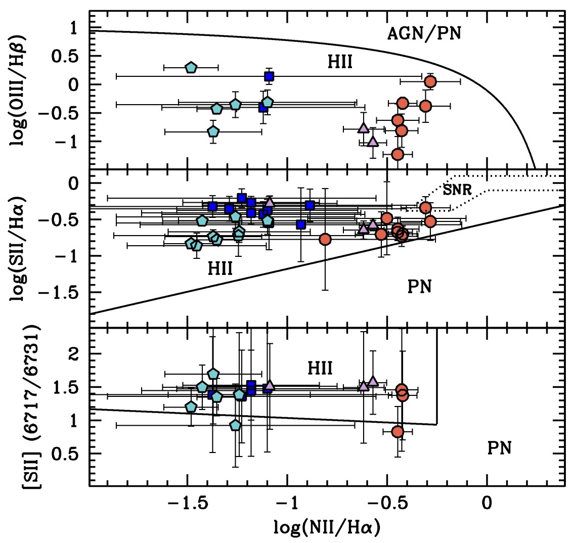
Figure 3: Line-ratio diagnostic diagrams for all the individual sources in which it was possible to measure the relevant line fluxes from MUSE spectra. The symbol coding is as follows: blue squares BC1, turquoise pentagons BC3, red circles BC4, plum triangles BC5. The lines separating different kind of sources in the diagrams are: Eq. 5 from Kewley et al. 2001 (upper panel), Eq. 3 from Kniazev et al. 2008 (middle panel), and Eq. 4 and 5 from the same source (lower panel). In the middle panel, a dotted line contour encloses the region of the diagram where Supernova Remnants (SNR) are expected to lie.

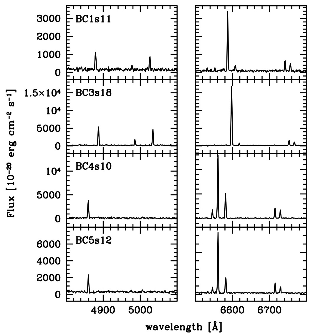
Figure 4: Spectra of the sources with the strongest H$\alpha$ lines in each BC. For each source, two portions of the MUSE spectra are shown, enclosing the most relevant emission lines: H$\beta$, [O iii]4959, [O iii]5007 (left panels), and [N ii]6548, H$\alpha$, [N ii]6583, and [S ii]6717$+$6731 (right panels).

The issue of the classification of the individual sources detected with Sextractor is addressed in Fig. 3, where three different diagnostic plots based on line ratios are presented for the (different) subsets of sources having measures of the flux in the involved lines. While the uncertainties are large in some cases, all the considered sources behave as H ii regions, the only possible exception being BC2s12L that lies just within the contour enclosing Supernova remnants in the middle panel of Fig. 3. We conclude that all the systems are actively forming stars, fully analogous to the case of SECCO 1. In Fig. 4 we show the spectra of the sources with the strongest H$\alpha$ line in each BC, to show the quality of the best spectra in our dataset.

Before proceeding with the analysis of the internal kinematics of the new stellar systems it may be worth putting them in context within the Virgo cluster of galaxies. In Fig. 5a, BC1, BC3, BC4, and BC5, together with SECCO 1, are shown in projection on a wide map of Virgo, as traced by the distribution of galaxies included in the Extended Virgo Cluster Catalog (EVCC; Kim et al., 2014). The main substructures of the cluster are labelled, following Boselli et al. (2014). Fig. 5b shows that all our targets have mean velocities (from Tab. 6) within the range spanned by EVCC galaxies, hence they are very likely members of the Virgo cluster, a conclusion that is also supported by HST data (Pap-II). In particular, BC1 and BC3 are consistent with membership to Cluster C, while SECCO 1, BC4 and BC5 may belong to LVC or to Cluster A. According to Boselli et al. (2014) all these substructures of Virgo have the same mean distance from us. In the following we will consider all the newly confirmed BCs and SECCO 1 as members of the Virgo cluster, adopting D=16.5 Mpc (Mei et al., 2007) for all of them, as done in Pap-II.

Figure 5: Location of the Blue Candidates and of SECCO 1 within the Virgo cluster. In panel (a) the position of the systems (blue diamonds) is indicated within a wide map of the Virgo cluster, as traced by the distribution of EVCC galaxies (small grey circles; Kim et al., 2014); the main substructures of the cluster are labelled, following (Boselli et al., 2014). In panel (b) EVCC galaxies (grey squares) and the BCs (encircled blue filled circles) are plotted into a phase-space diagram opposing the heliocentric line of sight velocity to the angular distance from M 87, taken as the center of the Virgo cluster.

Figure 6: Radial velocity fields, in RA [deg] and Dec [deg] of the four systems, as traced by the individual H ii sources. BC4L and BC4R sources are shown in the same map. The source at the South-Eastern corner of panel (d) is BC5s3, not shown in Fig. 2c.

In Fig. 6, the maps of all the individual sources detected with Sextractor are shown for all the considered systems, color coded according to the source RV. BC4L and BC4R are shown in the same map; their proximity and similar RV indicate their common origin. In each BC the star forming sources have the same RV within a few tens of ${\rm\,km\,s^{-1}}$ indicating that all are part of the same system, having a common origin, which is also confirmed by their chemical homogeneity (see Sect. 4). In all cases, some sign of kinematic coherence of sub-groups of adjacent sources is perceivable, suggesting that the systems are structured into clumps, that, possibly, are slowly flying apart one from the other (see below). To make a direct comparison between the physical size and the kinematics of the various systems, including RV uncertainties, in Fig. 7 we plot the projected distance from the center of the system (along the right ascension direction, RA offset) and radial velocity of each individual source. The adopted centers are listed in Tab. 6. BC4L and BC4R are shown separately (middle panels of Fig. 7) and together in a single panel (lower left panel). The observed configurations suggest different degrees of spatial and kinematic coherence, with some hints of velocity gradients. In particular the diagram showing the two pieces of BC4 together may suggest the case of a system moving toward us, lead by the dense clump around RA offset$=-2$ kpc, while sources to both sides of it are lagging behind proportionally to their physical distance, reminiscent of the configuration produced in the simulation with star-formation by Calura et al. (2020, see their Fig. 11).

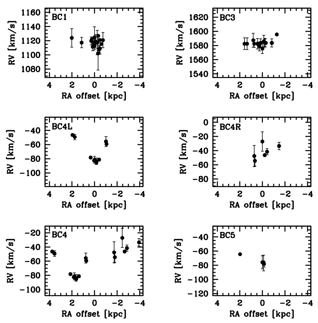
Figure 7: Projected distance from the center of the system along the RA direction ( RA offset; East is toward the left) vs. radial velocity for BC1, BC3, BC4L, BC4R, BC4 as a whole, and BC5, from top to bottom and from left to right, respectively.

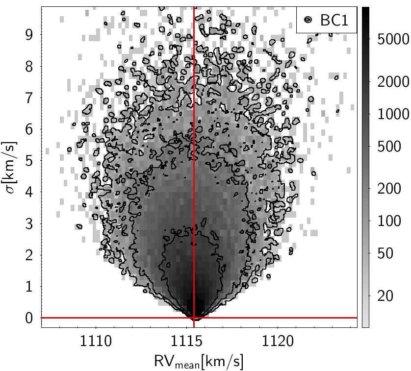
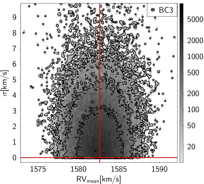
Figure 8: 2D posteriori PDF of $RV_{mean}$ and $\sigma_{int}$ as sampled with MCMC, for BC1 and BC3. The red vertical line marks the median of the $RV_{mean}$ distribution, while the red horizontal line marks the mode of the $\sigma_{int}$ distribution.

The RV distributions displayed in Fig. 6 and Fig. 7 suggest that a simple velocity dispersion is probably not adequate to capture the internal kinematics of these systems. The $\sigma$ values listed in Tab. 6 are standard deviations, not corrected for observational uncertainties. These are of the order of the uncertainties on individual RV estimates, suggesting that the velocity dispersions are not resolved by our data. To have a deeper insight into this problem we make an attempt to estimate the intrinsic dispersion for the two systems showing both the highest degree of kinematic coherence and the largest number of individual sources, BC1 and BC3. To have reliable uncertainties associated to each RV estimate we selected only sources whose RV and $\epsilon RV$ were obtained from at least three different spectral lines, thus selecting samples of 13 and 12 sources for BC1 and BC3, respectively.

From these data we derived the Probability Density Function (PDF) of the parameters of a simple Gaussian model ($V_{sys}$, $\sigma_{int}$) through a Bayesian analysis, using a Monte Carlo Markov Chain (MCMC) analysis, as done in Bellazzini et al. (2019). We used JAGS, within the R environment, to run four independent MCMCs of 10000 steps each, after a burn in phase of 1000 steps. For both parameters uniform priors were adopted: for $V_{sys}$ in a range of $\simeq\pm 50{\rm\,km\,s^{-1}}$ around the mean RV, for $\sigma_{int}$ in the range $0.0{\rm\,km\,s^{-1}}<\sigma_{int}<10.0{\rm\,km\,s^{-1}}$. The resulting 2D PDFs, as sampled by MCMCs, are shown in Fig. 8. The median ($P_{50}$) $\pm$ the semi-difference between 16th and 84th percentiles of the marginalised $V_{sys}$ PDF are $P_{50}=1115.4\pm 1.2{\rm\,km\,s^{-1}}$ for BC1, and $P_{50}=1582.6\pm 2.1{\rm\,km\,s^{-1}}$ for BC3, in agreement, within the uncertainty, with the straight averages listed in Tab. 6. On the other hand, Fig. 8 clearly demonstrates that the velocity dispersions are unresolved by our data, even in these most favourable cases. For both systems the PDF reaches its maximum at $\sigma_{int}=0.0{\rm\,km\,s^{-1}}$. For BC1(BC3) half of the points sampling the PDF have $\sigma_{int}\leq 1.7(1.6){\rm\,km\,s^{-1}}$, 75% have $\sigma_{int}\leq 3.0(2.8){\rm\,km\,s^{-1}}$, and 95% have $\sigma_{int}\leq 5.6(5.1){\rm\,km\,s^{-1}}$. It can be concluded that BC1 and BC3 may have $\sigma_{int}$ virtually anywhere between $\simeq 0{\rm\,km\,s^{-1}}$ and $\simeq 6{\rm\,km\,s^{-1}}$, but most likely $\sigma_{int}\leq 3.0{\rm\,km\,s^{-1}}$.

Calura et al. (2020) introduced a stellar virial ratio ($\alpha_{vir}$, their Eq. 8) as a simple parameter to evaluate if a stellar system is gravitationally bound ($\alpha_{vir}\lesssim 1$) or not ($\alpha_{vir}\gg 1$). We can use the version of their equation having the half light radius ($R_{h}$) as input parameter, instead of the 3D half-mass radius, to estimate $\alpha_{vir}$ for the BCs. Pap-II estimates for these systems stellar masses in the range $4\times 10^{4}~{}M_{\odot}-1\times 10^{5}~{}M_{\odot}$. Assuming, conservatively, $M=10^{5}~{}M_{\odot}$, taking $R_{med}$ from Tab. 6 as a proxy for $R_{h}$, and adopting $\sigma_{int}=1.0{\rm\,km\,s^{-1}}$ we obtain $\alpha_{vir}=6.9,11.7,7.4,6.8,4.2$, for BC1, BC3, BC4L, BC4R, and BC5, respectively. Assuming $\sigma_{int}=2.0{\rm\,km\,s^{-1}}$ will move all the $\alpha_{vir}$ to values in the range $15-50$, while keeping $\sigma_{int}=1.0{\rm\,km\,s^{-1}}$ and assuming $M=10^{6}~{}M_{\odot}$ would imply $\alpha_{vir}\lesssim 1$ for all the systems. We conclude that BC1, BC3, BC4L, BC4R, and BC5 are most likely unbound, as stellar systems. However they can be considered somehow borderline, given the sizeable uncertainties in all the parameters involved in the computation of $\alpha_{vir}$ and the inadequacy of a simple gaussian to model their velocity distribution. It is quite possible that some of the sub-clumps they are made of would leave a bound remnant, a small open cluster -like system floating undisturbed within Virgo, while its stars evolve passively (an hypothesis already suggested by Bellazzini et al., 2018).

4 Metallicity and star formation

Given the available lines with measured fluxes, corrected for extinction, we estimated the gas phase oxygen abundance using two different strong-line ratios, N2=[Nii]/H$\alpha$, and O3N2=([Oiii]/H$\beta$)/([Nii]/H$\alpha$), as defined by Pettini & Pagel (2004, PP04 hereafter). We were able to measure N2 for the 35 sources listed in Table 5 and O3N2 for 15 of them. In Tab. 5 we provide the values of $12+{\rm log}(O/H)$ derived from N2 and O3N2 using both the calibration by PP04 and by Marino et al. (2013, M13 hereafter). The individual errors on the oxygen abundance of each region properly include the contribution of the uncertainties on the fluxes of the emission lines and on their correction for reddening, as well as of the uncertainty associated to the adopted calibrations. Following Be17, to compensate for the effects of varying ionisation, we compute the oxygen abundance as the average of the abundances from N2 and O3N2 (N2+03N2), taking the average from the PP04 calibrations as our preferred value. The mean abundances of the studied systems range from $12+{\rm log}(O/H)=8.29\pm 0.10$ to $12+{\rm log}(O/H)=8.73\pm 0.04$ (Tab. 6), clearly much larger than expected values for galaxies with such a low stellar mass, that typically have $12+{\rm log}(O/H)\leq 7.5$ (see. e.g., Hidalgo, 2017). This indicates that these systems have likely originated from gas stripped from larger galaxies, like SECCO 1 (see Pap-II for a deeper discussion).

The mean abundance and standard deviations reported in Tab. 6 are obtained from N2+03N2, hence they are limited to the few sources per system having estimates of O3N2. However, we can use the abundances from N2 (PP04 calibration), that are available for many more sources, to have a more realistic estimate of the uncertainties on the mean abundances and to study the chemical homogeneity of the various BCs. Unfortunately, the uncertainty on the abundance of individual sources can be quite large, ranging from $0.09$ dex to $0.9$ dex, providing poor constraints on the abundance spread, especially for BC1, where even the brightest sources have relatively low signal to noise spectra. As in the case of velocity dispersion, also the metallicity dispersion is not resolved by our data. However we can attempt to obtain some collective constraint on the intrinsic dispersion.

Using the simple Maximum Likelihood algorithm described by Mucciarelli et al. (2012), we find mean oxygen abundances of $\langle 12+{\rm log}(O/H)\rangle=8.3\pm 0.2,8.2\pm 0.1,8.66\pm 0.04$, and $8.56\pm 0.07$, for BC1, BC3, BC4 and BC5, respectively. In all cases the most likely value for the intrinsic dispersion is zero, with 1$\sigma$ uncertainties ranging from $0.04$ dex (BC4, from 13 sources) to $0.2$ dex (BC1, from 10 sources). We conclude: a) that the typical internal uncertainties for the mean abundances range from 0.04 dex to 0.2 dex, and b) that all the systems appear as remarkably homogeneous from the chemical point of view, again similar to SECCO 1. This supports the view that all the H ii regions within a given BC were born from the same gas cloud. The fact that these sources were born together and now lie in clumps between $\sim 1-8$  kpc (in projection) from each other may suggest that they are in the process of dissolving.

Finally, in Tab. 6 we report also the estimates of the total integrated H$\alpha$ flux for each BC, obtained by photometry with large apertures on the continuum-subtracted images shown in Fig. 1 and Fig. 2. Once corrected for the average extinction using the extinction law by Calzetti et al. (2000) with $R_{V}=3.1$, the integrated fluxes can be can be converted into estimates of the current Star Formation Rate (SFR) using Eq. 2 of Kennicutt (1998). SFR for the considered systems ranges from $\simeq 0.3\times 10^{-3}M_{\odot}~{}yr^{-1}$ (BC1, BC5) to $\simeq 1.7\times 10^{-3}M_{\odot}~{}yr^{-1}$ (BC3), to be compared with $\simeq 0.7\times 10^{-3}M_{\odot}~{}yr^{-1}$ of SECCO 1, lying in the same range (Bellazzini et al., 2018).

5 Summary and conclusions

We have presented the results of MUSE observations of five candidate isolated star forming regions, optically selected to be similar to the prototype of the class SECCO 1. The acquired spectra allowed us to reject one of the candidates (BC2) and to confirm the other four (BC1, BC3, BC4, and BC5) as genuine star forming regions, likely lying in the Virgo cluster of galaxies (see Pap-II for additional support to this conclusion). All the physical properties that we were able to measure are similar to those observed in SECCO 1. In particular:

• in all the confirmed BCs we identified several H ii regions, plus some diffuse hot gas.

• The mean heliocentric velocity of each BC is consistent with membership in the Virgo cluster.

• Each BC is typically composed of a few, separated, star forming clumps, with systemic velocities within, at most, a few tens of ${\rm\,km\,s^{-1}}$. In the case of the most extended system, BC4, velocity gradients suggesting ongoing disruption are observed.

• Our velocity estimates do not have a sufficient precision to resolve the velocity dispersion of the considered systems, that, however, should be, in all cases $\sigma\lesssim 20~{}{\rm\,km\,s^{-1}}$ . Still, given the available constraints, it seems unlikely that they can survive as gravitationally bound stellar systems.

• The mean oxygen abundance of each BC is significantly larger than that expected for galaxies of similar stellar mass, strongly suggesting that they originated from gas clouds stripped from larger galaxies. Each BC appears internally homogeneous in terms of oxygen abundance, within the limits of the available observation, suggesting that all the associated sources were born from the same gas cloud.

• The instantaneous SFR is $0.3\times 10^{-3}M_{\odot}~{}yr^{-1}\lesssim{\rm SFR}\lesssim 2.0\times 10^{-3}M_{\odot}~{}yr^{-1}$.

These results, together with those obtained from HST and Hi observations are discussed in the companion paper Pap-II, where an evolutionary path for the studied system is proposed.

Table 2: Position, radial velocity and observed H$\alpha$ flux of individual sources

name	ra	dec	RV	$\epsilon$RV	NRV	F(H$\alpha$)	$\epsilon$F(H$\alpha$)	FWHM
	[deg]	[deg]	[km s-1]	[km s-1]		[10-18 erg cm-2 s-1]	[10-18 erg cm-2 s-1]	arcsec
BC1s11	189.75810	12.20365	1111.3	5.5	7	97.6	7.9	2.2
BC1s12	189.75754	12.20245	1113.4	6.3	5	58.8	5.9	8.2
BC1s13	189.76160	12.20350	1117.3	7.3	5	69.0	6.5	2.4
BC1s14	189.75489	12.20448	1120.8	10.8	4	23.4	4.2	1.5
BC1s15	189.75585	12.20327	1109.1	8.1	5	49.6	5.5	3.6
BC1s17	189.75859	12.20172	1119.7	5.6	4	14.1	3.7	1.2
BC1s20	189.75723	12.20065	1119.0	9.5	5	40.8	5.0	2.9
BC1s57W†	189.75637	12.20567	1126.9	20.0	1	9.4	3.0	1.3
BC1s61W†	189.75583	12.20534	1120.9	20.0	1	8.6	3.0	0.5
BC1s62W†	189.75534	12.20506	1115.4	20.0	1	8.4	3.4	0.6
BC1s65W†	189.76471	12.20468	1124.0	13.0	3	11.7	3.6	1.7
BC1s67W†	189.75644	12.20414	1102.0	23.4	2	8.3	3.4	1.5
BC1s73W	189.75604	12.20332	1108.0	5.2	5	43.6	5.2	2.6
BC1s80W	189.75777	12.20287	1115.5	2.0	4	57.4	5.9	4.0
BC1s83W	189.75667	12.20241	1117.3	17.2	4	13.5	3.7	0.9
BC1s90W	189.75751	12.20178	1117.7	6.6	4	55.0	5.8	1.7
BC1s92W	189.75840	12.20138	1121.9	20.0	1	15.3	3.8	0.5
BC1s98W	189.75757	12.20055	1124.6	15.1	4	29.5	4.5	1.4
BC3s4	191.67637	10.37416	1575.7	7.2	5	219.7	14.0	5.3
BC3s9	191.67924	10.37005	1587.4	9.9	4	167.2	11.4	2.7
BC3s10	191.67892	10.36901	1582.6	5.3	7	465.3	26.3	1.9
BC3s12	191.67594	10.36945	1586.0	8.5	4	33.4	4.7	2.4
BC3s13	191.67792	10.36832	1582.5	7.4	5	62.6	6.1	1.7
BC3s14	191.67730	10.36820	1578.7	6.2	3	24.9	4.2	1.5
BC3s15	191.67549	10.36701	1583.7	5.8	7	390.4	22.5	3.6
BC3s16	191.67691	10.36682	1583.7	5.8	7	63.1	6.2	4.3
BC3s18	191.67344	10.36558	1583.7	5.8	7	489.6	27.5	1.6
BC3s19	191.68198	10.36358	1582.5	8.3	5	68.4	6.4	5.2
BC3s20	191.68117	10.36314	1582.5	8.3	5	53.0	5.7	3.3
BC3s23	191.67339	10.36230	1583.6	20.0	1	12.5	3.6	0.7
BC3s24W	191.67529	10.37407	1583.6	20.0	1	27.4	4.4	1.4
BC3s26W	191.67561	10.37388	1584.1	5.8	4	49.6	5.5	1.2
BC3s69W	191.67186	10.36344	1595.6	20.0	1	12.5	3.5	1.1
BC4s3L	186.60278	14.39644	-55.7	7.1	5	10.7	3.5	1.1
BC4s4L	186.60263	14.39481	-59.4	1.1	5	121.9	9.1	1.2
BC4s8L	186.60766	14.38708	-78.3	1.7	7	143.3	10.2	1.2
BC4s9L	186.60658	14.38645	-82.6	1.3	6	89.0	7.4	1.8
BC4s10L	186.60584	14.38589	-85.2	1.6	6	149.8	10.5	2.6
BC4s11L	186.61344	14.38647	-46.5	1.8	6	49.8	5.5	1.5
BC4s12L	186.61272	14.38597	-49.3	3.9	6	44.9	5.2	4.2
BC4s13L	186.60643	14.38496	-81.4	4.9	3	6.7	3.3	1.2
BC4s14L	186.60498	14.38439	-81.3	2.0	3	17.8	3.9	2.1
continue

Table 2: continued

name	ra	dec	RV	$\epsilon$RV	NRV	F(H$\alpha$)	$\epsilon$F(H$\alpha$)	FWHM
	[deg]	[deg]	[km s-1]	[km s-1]		[10-18 erg cm-2 s-1]	[10-18 erg cm-2 s-1]	arcsec
BC4s38WL	186.60586	14.38522	-83.6	4.6	5	19.7	4.0	1.6
BC4s11R	186.58587	14.39747	-33.4	5.2	5	8.1	3.4	0.9
BC4s12R	186.59377	14.39739	-47.6	15.0	3	11.4	3.6	0.9
BC4s15R	186.59044	14.39478	-46.4	1.3	6	67.7	6.4	2.8
BC4s34WR	186.59354	14.39690	-54.4	7.3	2	4.8	3.2	1.5
BC4s40WR	186.58970	14.39530	-41.6	4.3	5	8.9	3.4	0.8
BC4s41WR	186.59118	14.39515	-27.1	13.6	2	8.4	3.4	1.3
BC5s3⋆	186.63569	15.16547	-64.4	20.0	1	39.7	5.0	.1.1
BC5s9	186.62805	15.17529	-78.2	4.1	5	111.7	8.6	2.9
BC5s10	186.62818	15.17447	-76.8	11.1	5	73.0	6.6	1.4
BC5s12	186.62856	15.17307	-75.8	9.2	6	213.0	13.7	4.1

Table 4: Line fluxes of individual sources, in units of the H$\beta$ flux, set to F(H$\beta$)=100.

Name	F(H$\beta$)	[OIII]5007	H$\alpha$	[NII]6584	[SII]6717	[SII]6731	Cβ
	[10-18 erg cm-2 s-1]						mag
BC1s11	8.1 $\pm$ 3.4	138.3 $\pm$45.2	299.4$\pm$97.2	24.3$\pm$ 42.0	49.8$\pm$ 48.0	34.7$\pm$ 44.7	1.99$\pm$0.21
BC1s12	13.6 $\pm$ 3.7	$\cdots$	290.5$\pm$43.7	23.1$\pm$ 23.8	73.1$\pm$ 27.7	49.6$\pm$ 25.9	0.57$\pm$0.16
BC1s13	21.8 $\pm$ 4.1	$\cdots$	287.8$\pm$29.6	19.0$\pm$ 14.8	94.1$\pm$ 19.0	61.6$\pm$ 17.2	0.14$\pm$0.12
BC1s14	6.9 $\pm$ 3.3	$\cdots$	288.4$\pm$60.3	37.5$\pm$ 45.5	91.0$\pm$ 48.7	51.8$\pm$ 46.4	0.23$\pm$0.28
BC1s15	11.9 $\pm$ 3.6	$\cdots$	290.2$\pm$46.0	17.2$\pm$ 26.4	103.9$\pm$ 32.8	76.5$\pm$ 30.8	0.52$\pm$0.18
BC1s17	4.0 $\pm$ 3.2	$\cdots$	288.8$\pm$92.8	$\cdots$	$\cdots$	$\cdots$	0.29$\pm$0.46
BC1s20	13.1 $\pm$ 3.7	$\cdots$	287.7$\pm$38.4	19.0$\pm$ 23.8	66.1$\pm$ 26.4	45.7$\pm$ 25.3	0.11$\pm$0.17
BC1s62W	6.4 $\pm$ 3.3	$\cdots$	131.1$\pm$53.5	$\cdots$	$\cdots$	$\cdots$	0.00$\pm$0.40
BC1s73W	7.3 $\pm$ 3.4	$\cdots$	293.3$\pm$70.8	18.4$\pm$ 42.9	109.6$\pm$ 52.7	68.6$\pm$ 48.4	1.01$\pm$0.25
BC1s80W	12.6 $\pm$ 3.6	39.4 $\pm$25.9	291.0$\pm$46.6	22.1$\pm$ 25.6	65.4$\pm$ 29.1	42.6$\pm$ 27.3	0.64$\pm$0.17
BC1s83W	3.7 $\pm$ 3.2	$\cdots$	288.9$\pm$98.0	10.0$\pm$ 80.7	170.1$\pm$ 90.8	93.3$\pm$ 86.0	0.31$\pm$0.48
BC1s90W	12.3 $\pm$ 3.6	$\cdots$	290.8$\pm$46.7	12.3$\pm$ 25.3	80.5$\pm$ 30.7	58.1$\pm$ 29.0	0.61$\pm$0.17
BC1s92W	5.0 $\pm$ 3.2	$\cdots$	287.6$\pm$75.3	33.7$\pm$ 61.7	42.9$\pm$ 62.2	34.2$\pm$ 61.8	0.09$\pm$0.38
BC1s98W	12.3 $\pm$ 3.6	$\cdots$	239.8$\pm$36.4	12.3$\pm$ 25.0	66.0$\pm$ 27.7	40.1$\pm$ 26.4	0.00$\pm$0.19
BC3s4	70.3 $\pm$ 6.5	$\cdots$	287.7$\pm$19.9	10.8$\pm$ 4.8	52.1$\pm$ 7.1	34.8$\pm$ 6.2	0.12$\pm$0.07
BC3s9	49.6 $\pm$ 5.5	14.7 $\pm$6.8	288.4$\pm$22.9	12.3$\pm$ 6.8	33.2$\pm$ 8.0	19.6$\pm$ 7.2	0.22$\pm$0.08
BC3s10	143.1 $\pm$10.1	37.1 $\pm$4.0	288.1$\pm$18.3	12.8$\pm$ 2.8	27.4$\pm$ 3.7	20.3$\pm$ 3.2	0.17$\pm$0.05
BC3s12	6.9 $\pm$ 3.3	$\cdots$	291.5$\pm$67.7	$\cdots$	$\cdots$	$\cdots$	0.73$\pm$0.27
BC3s13	13.4 $\pm$ 3.7	$\cdots$	291.1$\pm$45.6	16.6$\pm$ 23.6	32.4$\pm$ 25.0	22.7$\pm$ 24.2	0.67$\pm$0.16
BC3s15	124.8 $\pm$ 9.2	195.1 $\pm$12.3	287.7$\pm$18.0	9.5$\pm$ 2.9	23.0$\pm$ 3.7	19.2$\pm$ 3.4	0.12$\pm$0.06
BC3s16	13.8 $\pm$ 3.7	48.4 $\pm$24.2	291.0$\pm$44.5	23.2$\pm$ 23.5	51.7$\pm$ 25.9	36.7$\pm$ 24.7	0.64$\pm$0.16
BC3s18	47.5 $\pm$ 5.4	$\cdots$	298.1$\pm$57.9	10.5$\pm$ 8.1	24.4$\pm$ 10.9	16.7$\pm$ 9.5	1.77$\pm$0.07
BC3s19	24.9 $\pm$ 4.2	$\cdots$	274.8$\pm$25.8	15.8$\pm$ 12.8	34.2$\pm$ 13.8	24.7$\pm$ 13.3	0.00$\pm$0.11
BC3s20	8.7 $\pm$ 3.4	$\cdots$	293.4$\pm$64.7	1.8$\pm$ 34.5	44.8$\pm$ 39.2	25.3$\pm$ 37.1	1.04$\pm$0.21
BC3s26W	14.4 $\pm$ 3.7	44.1 $\pm$23.0	288.5$\pm$37.9	15.9$\pm$ 21.7	47.7$\pm$ 23.6	51.7$\pm$ 23.9	0.25$\pm$0.16
BC4s4L	31.0 $\pm$ 4.6	15.4 $\pm$10.5	289.7$\pm$29.3	108.4$\pm$ 17.0	31.9$\pm$ 11.9	21.9$\pm$ 11.2	0.43$\pm$0.09
BC4s8L	38.6 $\pm$ 4.9	46.6 $\pm$10.2	289.3$\pm$26.3	109.5$\pm$ 14.8	33.5$\pm$ 10.0	24.4$\pm$ 9.4	0.36$\pm$0.08
BC4s9L	20.9 $\pm$ 4.0	23.5 $\pm$15.6	290.5$\pm$35.6	104.0$\pm$ 22.0	39.8$\pm$ 17.3	28.2$\pm$ 16.5	0.54$\pm$0.12
BC4s10L	39.0 $\pm$ 4.9	5.9 $\pm$ 8.0	289.6$\pm$26.9	103.5$\pm$ 14.6	27.6$\pm$ 9.6	33.3$\pm$ 10.0	0.40$\pm$0.08
BC4s11L	9.8 $\pm$ 3.5	111.7 $\pm$36.5	292.0$\pm$55.9	152.1$\pm$ 43.8	53.4$\pm$ 35.4	33.0$\pm$ 33.5	0.79$\pm$0.20
BC4s12L	12.0 $\pm$ 3.6	41.6 $\pm$27.1	289.3$\pm$43.7	142.6$\pm$ 34.2	81.3$\pm$ 30.3	51.4$\pm$ 28.4	0.37$\pm$0.18
BC4s14L	5.7 $\pm$ 3.3	$\cdots$	287.8$\pm$68.8	44.6$\pm$ 55.5	28.6$\pm$ 54.6	19.8$\pm$ 54.1	0.13$\pm$0.34
BC4s38WL	4.2 $\pm$ 3.2	$\cdots$	291.3$\pm$94.2	91.9$\pm$ 78.3	60.3$\pm$ 75.7	35.2$\pm$ 73.8	0.67$\pm$0.41
BC4s15R	17.3 $\pm$ 3.9	$\cdots$	289.7$\pm$36.9	85.6$\pm$ 23.1	38.1$\pm$ 19.9	19.1$\pm$ 35.0	0.43$\pm$0.14
BC5s9	29.4 $\pm$ 4.5	16.4 $\pm$11.0	289.4$\pm$29.2	69.9$\pm$ 14.8	39.3$\pm$ 12.8	26.3$\pm$ 12.0	0.39$\pm$0.10
BC5s10	18.2 $\pm$ 3.9	$\cdots$	289.9$\pm$36.6	23.7$\pm$ 18.1	91.4$\pm$ 23.0	60.5$\pm$ 20.79	0.46$\pm$0.13
BC5s12	56.7 $\pm$ 5.8	9.4 $\pm$5.8	289.3$\pm$24.1	77.7$\pm$ 10.3	46.2$\pm$ 8.3	29.5$\pm$ 7.24	0.37$\pm$0.07

Table 5: Metallicity of individual sources.

Name	12+log(O/H)	12+log(O/H)	$\langle{\rm 12+{\rm log}(O/H)}\rangle$	12+log(O/H)	12+log(O/H)	$\langle{\rm 12+{\rm log}(O/H)}\rangle$
	N2(PP04)	O3N2(PP04)	N2+O3N2(PP04)	N2(M13)	O3N2(M13)	N2+O3N2(M13)
BC1s11	8.28$\pm$0.88	8.33$\pm$ 1.02	8.31$\pm$ 0.90	8.24$\pm$ 0.88	8.27$\pm$ 1.02	8.26$\pm$ 0.89
BC1s12	8.27$\pm$0.50	$\cdots$	$\cdots$	8.24$\pm$ 0.50	$\cdots$	$\cdots$
BC1s13	8.23$\pm$0.37	$\cdots$	$\cdots$	8.20$\pm$ 0.37	$\cdots$	$\cdots$
BC1s14	8.39$\pm$0.61	$\cdots$	$\cdots$	8.33$\pm$ 0.61	$\cdots$	$\cdots$
BC1s15	8.20$\pm$0.72	$\cdots$	$\cdots$	8.18$\pm$ 0.72	$\cdots$	$\cdots$
BC1s20	8.23$\pm$0.59	$\cdots$	$\cdots$	8.20$\pm$ 0.59	$\cdots$	$\cdots$
BC1s80W	8.26$\pm$0.56	8.50$\pm$ 0.84	8.38$\pm$ 0.60	8.23$\pm$ 0.56	8.38$\pm$ 0.84	8.30$\pm$ 0.59
BC1s90W	8.12$\pm$0.95	$\cdots$	$\cdots$	8.11$\pm$ 0.95	$\cdots$	$\cdots$
BC1s92W	8.37$\pm$0.90	$\cdots$	$\cdots$	8.31$\pm$ 0.90	$\cdots$	$\cdots$
BC1s98W	8.17$\pm$0.93	$\cdots$	$\cdots$	8.15$\pm$ 0.93	$\cdots$	$\cdots$
BC3s4	8.09$\pm$0.22	$\cdots$	$\cdots$	8.09$\pm$ 0.22	$\cdots$	$\cdots$
BC3s9	8.12$\pm$0.27	8.55$\pm$ 0.47	8.34$\pm$ 0.33	8.11$\pm$ 0.27	8.42$\pm$ 0.47	8.26$\pm$ 0.32
BC3s10	8.13$\pm$0.12	8.43$\pm$ 0.16	8.28$\pm$ 0.23	8.12$\pm$ 0.12	8.34$\pm$ 0.16	8.23$\pm$ 0.20
BC3s13	8.19$\pm$0.67	$\cdots$	$\cdots$	8.17$\pm$ 0.67	$\cdots$	$\cdots$
BC3s15	8.06$\pm$0.15	8.16$\pm$ 0.18	8.11$\pm$ 0.25	8.06$\pm$ 0.15	8.16$\pm$ 0.18	8.11$\pm$ 0.23
BC3s16	8.28$\pm$0.50	8.48$\pm$ 0.71	8.38$\pm$ 0.54	8.24$\pm$ 0.50	8.37$\pm$ 0.71	8.30$\pm$ 0.52
BC3s18	8.07$\pm$0.41	$\cdots$	$\cdots$	8.07$\pm$ 0.41	$\cdots$	$\cdots$
BC3s19	8.19$\pm$0.38	$\cdots$	$\cdots$	8.17$\pm$ 0.38	$\cdots$	$\cdots$
BC3s26W	8.18$\pm$0.64	8.44$\pm$ 0.86	8.31$\pm$ 0.67	8.16$\pm$ 0.64	8.34$\pm$ 0.86	8.25$\pm$ 0.66
BC4s4L	8.65$\pm$0.11	8.85$\pm$ 0.40	8.75$\pm$ 0.22	8.54$\pm$ 0.11	8.61$\pm$ 0.4	8.58$\pm$ 0.20
BC4s8L	8.66$\pm$0.09	8.70$\pm$ 0.19	8.68$\pm$ 0.22	8.54$\pm$ 0.09	8.51$\pm$ 0.19	8.53$\pm$ 0.19
BC4s9L	8.64$\pm$0.14	8.78$\pm$ 0.42	8.71$\pm$ 0.24	8.53$\pm$ 0.14	8.57$\pm$ 0.42	8.55$\pm$ 0.22
BC4s10L	8.64$\pm$0.1	8.97$\pm$ 0.68	8.81$\pm$ 0.22	8.53$\pm$ 0.1	8.69$\pm$ 0.68	8.61$\pm$ 0.19
BC4s11L	8.74$\pm$0.20	8.62$\pm$ 0.34	8.68$\pm$ 0.28	8.61$\pm$ 0.20	8.46$\pm$ 0.34	8.53$\pm$ 0.26
BC4s12L	8.72$\pm$0.16	8.75$\pm$ 0.44	8.73$\pm$ 0.26	8.60$\pm$ 0.16	8.54$\pm$ 0.44	8.57$\pm$ 0.23
BC4s13L	8.79$\pm$0.12	$\cdots$	$\cdots$	8.66$\pm$ 0.12	$\cdots$	$\cdots$
BC4s14L	8.44$\pm$0.63	$\cdots$	$\cdots$	8.37$\pm$ 0.63	$\cdots$	$\cdots$
BC4s38WL	8.61$\pm$0.12	$\cdots$	$\cdots$	8.51$\pm$ 0.12	$\cdots$	$\cdots$
BC4s3L	8.60$\pm$0.12	$\cdots$	$\cdots$	8.50$\pm$ 0.12	$\cdots$	$\cdots$
BC4s15R	8.60$\pm$0.17	$\cdots$	$\cdots$	8.50$\pm$ 0.17	$\cdots$	$\cdots$
BC4s34WR	8.59$\pm$0.12	$\cdots$	$\cdots$	8.49$\pm$ 0.12	$\cdots$	$\cdots$
BC4s40WR	8.67$\pm$0.12	$\cdots$	$\cdots$	8.56$\pm$ 0.12	$\cdots$	$\cdots$
BC5s9	8.55$\pm$0.13	8.78$\pm$ 0.42	8.66$\pm$ 0.24	8.46$\pm$ 0.13	8.56$\pm$ 0.42	8.51$\pm$ 0.21
BC5s10	8.28$\pm$0.38	$\cdots$	$\cdots$	8.24$\pm$ 0.38	$\cdots$	$\cdots$
BC5s12	8.57$\pm$0.09	8.87$\pm$ 0.35	8.72$\pm$ 0.22	8.48$\pm$ 0.09	8.62$\pm$ 0.35	8.55$\pm$ 0.19

Table 6: Mean properties of the studied targets

name	RAJ2000	DecJ2000	Rmed	Rmax	Fint(H$\alpha$)	RV	$\sigma_{RV}$	NRV	$\langle 12+{\rm log}(O/H)\rangle$	$\sigma_{(O/H)}$	N(O/H)
	deg	deg	arcsec	arcsec	erg cm-2 s-1	km s-1	km s-1
BC1	189.75754	12.20332	8.3	28.1	5.5E-16	1117	6	18	8.35	0.04(0.2)	2(10)
BC3	191.67637	10.36820	14.0	25.9	31.3E-16	1584	4	15	8.29	0.09(0.1)	5(9)
BC4L	186.60643	14.38645	8.9	38.1	18.9E-16	-70	16	10	8.73	0.04(0.05)	6(10)
BC4R	186.59117	14.39690	8.2	18.6	4.0E-16	-42	10	6	$\cdots$	(0.08)	0(3)
BC4	186.60000	14.39000	33.5	56.1	23.0E-16	-60	20	16	8.73	0.04(0.04)	6(13)
BC5	186.62856	15.17447	5.0	40.8	5.7E-16	-74	6	4	8.70	0.03(0.08)	2(3)

References

- Adams et al. (2013) Adams, E. A. K., Giovanelli, R., & Haynes, M. P. 2013, ApJ, 768, 77, doi: 10.1088/0004-637X/768/1/77
- Adams et al. (2015) Adams, E. A. K., Cannon, J. M., Rhode, K. L., et al. 2015, A&A, 580, A134, doi: 10.1051/0004-6361/201526857
- Bacon et al. (2014) Bacon, R., Vernet, J., Borisova, E., et al. 2014, The Messenger, 157, 13
- Beccari et al. (2016) Beccari, G., Bellazzini, M., Battaglia, G., et al. 2016, A&A, 591, A56, doi: 10.1051/0004-6361/201527707
- Beccari et al. (2017) Beccari, G., Bellazzini, M., Magrini, L., et al. 2017, MNRAS, 465, 2189, doi: 10.1093/mnras/stw2874 (Be17)
- Bellazzini et al. (2019) Bellazzini, M., Ibata, R. A., Martin, N., et al. 2019, MNRAS, 490, 2588, doi: 10.1093/mnras/stz2788
- Bellazzini et al. (2015a) Bellazzini, M., Beccari, G., Battaglia, G., et al. 2015a, A&A, 575, A126, doi: 10.1051/0004-6361/201425262
- Bellazzini et al. (2015b) Bellazzini, M., Magrini, L., Mucciarelli, A., et al. 2015b, ApJ, 800, L15, doi: 10.1088/2041-8205/800/1/L15
- Bellazzini et al. (2018) Bellazzini, M., Armillotta, L., Perina, S., et al. 2018, MNRAS, 476, 4565, doi: 10.1093/mnras/sty467
- Bennet et al. (2022) Bennet, P., Sand, D. J., Crnojević, D., et al. 2022, ApJ, 924, 98, doi: 10.3847/1538-4357/ac356c
- Bertin & Arnouts (1996) Bertin, E., & Arnouts, S. 1996, A&AS, 117, 393, doi: 10.1051/aas:1996164
- Boselli et al. (2021) Boselli, A., Fossati, M., & Sun, M. 2021, arXiv e-prints, arXiv:2109.13614. https://arxiv.org/abs/2109.13614
- Boselli et al. (2014) Boselli, A., Voyer, E., Boissier, S., et al. 2014, A&A, 570, A69, doi: 10.1051/0004-6361/201424419
- Burkhart & Loeb (2016) Burkhart, B., & Loeb, A. 2016, ApJ, 824, L7, doi: 10.3847/2041-8205/824/1/L7
- Calura et al. (2020) Calura, F., Bellazzini, M., & D’Ercole, A. 2020, MNRAS, 499, 5873, doi: 10.1093/mnras/staa3133
- Calzetti et al. (2000) Calzetti, D., Armus, L., Bohlin, R. C., et al. 2000, ApJ, 533, 682, doi: 10.1086/308692
- Cannon et al. (2015) Cannon, J. M., Martinkus, C. P., Leisman, L., et al. 2015, AJ, 149, 72, doi: 10.1088/0004-6256/149/2/72
- Caplan & Deharveng (1986) Caplan, J., & Deharveng, L. 1986, A&A, 155, 297
- Corbelli et al. (2021a) Corbelli, E., Cresci, G., Mannucci, F., Thilker, D., & Venturi, G. 2021a, ApJ, 908, L39, doi: 10.3847/2041-8213/abdf64
- Corbelli et al. (2021b) Corbelli, E., Mannucci, F., Thilker, D., Cresci, G., & Venturi, G. 2021b, A&A, 651, A77, doi: 10.1051/0004-6361/202140398
- Fossati et al. (2016) Fossati, M., Fumagalli, M., Boselli, A., et al. 2016, MNRAS, 455, 2028, doi: 10.1093/mnras/stv2400
- Fumagalli et al. (2014) Fumagalli, M., Fossati, M., Hau, G. K. T., et al. 2014, MNRAS, 445, 4335, doi: 10.1093/mnras/stu2092
- Fumagalli et al. (2011) Fumagalli, M., Gavazzi, G., Scaramella, R., & Franzetti, P. 2011, A&A, 528, A46, doi: 10.1051/0004-6361/201015463
- Gerhard et al. (2002) Gerhard, O., Arnaboldi, M., Freeman, K. C., & Okamura, S. 2002, ApJ, 580, L121, doi: 10.1086/345657
- Giovanelli et al. (2013) Giovanelli, R., Haynes, M. P., Adams, E. A. K., et al. 2013, AJ, 146, 15, doi: 10.1088/0004-6256/146/1/15
- Hidalgo (2017) Hidalgo, S. L. 2017, A&A, 606, A115, doi: 10.1051/0004-6361/201630264
- Jones et al. (2022a) Jones, M. G., Sand, D. J., Bellazzini, M., et al. 2022a, ApJ in press, arXiv:2205.01695 (Pap-II)
- Jones et al. (2022b) —. 2022b, ApJ, 926, L15, doi: 10.3847/2041-8213/ac51dc
- Junais et al. (2021) Junais, Boissier, S., Boselli, A., et al. 2021, A&A, 650, A99, doi: 10.1051/0004-6361/202040185
- Kapferer et al. (2009) Kapferer, W., Sluka, C., Schindler, S., Ferrari, C., & Ziegler, B. 2009, A&A, 499, 87, doi: 10.1051/0004-6361/200811551
- Kenney et al. (2014) Kenney, J. D. P., Geha, M., Jáchym, P., et al. 2014, ApJ, 780, 119, doi: 10.1088/0004-637X/780/2/119
- Kennicutt (1998) Kennicutt, Robert C., J. 1998, ARA&A, 36, 189, doi: 10.1146/annurev.astro.36.1.189
- Kim et al. (2014) Kim, S., Rey, S.-C., Jerjen, H., et al. 2014, ApJS, 215, 22, doi: 10.1088/0067-0049/215/2/22
- Lupton & Monger (1991) Lupton, R., & Monger, P. 1991, SuperMongo
- Marino et al. (2013) Marino, R. A., Rosales-Ortega, F. F., Sánchez, S. F., et al. 2013, A&A, 559, A114, doi: 10.1051/0004-6361/201321956 (M13)
- McQuinn et al. (2015) McQuinn, K. B. W., Skillman, E. D., Dolphin, A., et al. 2015, ApJ, 812, 158, doi: 10.1088/0004-637X/812/2/158
- Mei et al. (2007) Mei, S., Blakeslee, J. P., Côté, P., et al. 2007, ApJ, 655, 144, doi: 10.1086/509598
- Mucciarelli et al. (2012) Mucciarelli, A., Bellazzini, M., Ibata, R., et al. 2012, MNRAS, 426, 2889, doi: 10.1111/j.1365-2966.2012.21847.x
- Nidever et al. (2019) Nidever, D. L., Price-Whelan, A. M., Choi, Y., et al. 2019, ApJ, 887, 115, doi: 10.3847/1538-4357/ab52fc
- Osterbrock & Ferland (2006) Osterbrock, D. E., & Ferland, G. J. 2006, Astrophysics of gaseous nebulae and active galactic nuclei
- Pasha et al. (2021) Pasha, I., Lokhorst, D., van Dokkum, P. G., et al. 2021, ApJ, 923, L21, doi: 10.3847/2041-8213/ac3ca6
- Pettini & Pagel (2004) Pettini, M., & Pagel, B. E. J. 2004, MNRAS, 348, L59, doi: 10.1111/j.1365-2966.2004.07591.x (PP04)
- Poggianti et al. (2019) Poggianti, B. M., Gullieuszik, M., Tonnesen, S., et al. 2019, MNRAS, 482, 4466, doi: 10.1093/mnras/sty2999
- Sand et al. (2015) Sand, D. J., Crnojević, D., Bennet, P., et al. 2015, ApJ, 806, 95, doi: 10.1088/0004-637X/806/1/95
- Sand et al. (2017) Sand, D. J., Seth, A. C., Crnojević, D., et al. 2017, ApJ, 843, 134, doi: 10.3847/1538-4357/aa7557
- Saul et al. (2012) Saul, D. R., Peek, J. E. G., Grcevich, J., et al. 2012, ApJ, 758, 44, doi: 10.1088/0004-637X/758/1/44
- Taylor (2005) Taylor, M. B. 2005, in Astronomical Society of the Pacific Conference Series, Vol. 347, Astronomical Data Analysis Software and Systems XIV, ed. P. Shopbell, M. Britton, & R. Ebert, 29
- Tody (1993) Tody, D. 1993, in Astronomical Society of the Pacific Conference Series, Vol. 52, Astronomical Data Analysis Software and Systems II, ed. R. J. Hanisch, R. J. V. Brissenden, & J. Barnes, 173
- Tollerud et al. (2015) Tollerud, E. J., Geha, M. C., Grcevich, J., Putman, M. E., & Stern, D. 2015, ApJ, 798, L21, doi: 10.1088/2041-8205/798/1/L21
- Weilbacher et al. (2012) Weilbacher, P. M., Streicher, O., Urrutia, T., et al. 2012, in Society of Photo-Optical Instrumentation Engineers (SPIE) Conference Series, Vol. 8451, Software and Cyberinfrastructure for Astronomy II, ed. N. M. Radziwill & G. Chiozzi, 84510B, doi: 10.1117/12.925114
- Yoshida et al. (2012) Yoshida, M., Yagi, M., Komiyama, Y., et al. 2012, ApJ, 749, 43, doi: 10.1088/0004-637X/749/1/43