Abstract

We present a Lohner-type algorithm for rigorous integration of systems of Delay Differential Equations (DDEs) with multiple delays, and its application in computation of Poincaré maps, to study the dynamics of some bounded, eternal solutions. The algorithm is based on a piecewise Taylor representation of the solutions in the phase-space and it exploits the smoothing of solutions occurring in DDEs to produces enclosures of solutions of a high order. We apply the topological techniques to prove various kinds of dynamical behaviour, for example, existence of (apparently) unstable periodic orbits in Mackey-Glass Equation (in the regime of parameters where chaos is numerically observed) and persistence of symbolic dynamics in a delay-perturbed chaotic ODE (the Rössler system).

AMS Subject Classification: 34K13, 34K23, 34K38, 65G20, 65Q20 Keywords: computer-assisted proofs, Periodic orbits, symbolic dynamics, covering relations, Fixed Point Index, infinite-dimensional phasespace

1 Introduction

We consider a system of Delay Differential Equations (DDEs) with constant delays and the initial condition of the following form:

$$\begin{cases}x^{\prime}(t)=f\left(x(t),x(t-\tau_{1}),x(t-\tau_{2}),\ldots,x(t-\tau_{m})\right),&t\geq 0\\ x(t)=\psi(t),&t\in[-\tau,0],\end{cases}$$ (1)

where $m\in\mathbb{N}$ and $\tau=\tau_{1}>\tau_{2}>\ldots>\tau_{m}\geq 0$ are the delays, $x^{\prime}$ is understood as a right derivative and $\psi:[-\tau,0]\to\mathbb{R}^{d}$ is of class $C^{0}$ on $[-\tau,0]$, $x(t)\in\mathbb{R}^{d}$, $f:\mathbb{R}^{(m+1)d}\to\mathbb{R}^{d}$.

In [34] we have presented a method of producing rigorous estimates on the function $x(t)$ for $t\geq 0$ for the simplest scalar ($d=1$) DDE with a single delay:

$$x^{\prime}(t)=f(x(t),x(t-\tau))\\$$ (2)

The algorithm presented in [34] is an explicit Taylor method with piecewise Taylor representation of the solution over a fixed step size grid and with Lohner-type control of the wrapping effect encountered in interval arithmetics [21]. The method consists of two algorithms: one computing Taylor coefficients of the solutions at equally spaced grid points (together with the rigorous estimate on the error size), and the second one to compute enclosures of the solution segment after an arbitrary step of size $\varepsilon$, smaller than the grid step size $h$. The method is suited to construct Poincaré maps in the phase space of the DDEs and it was successfully applied to prove several (apparently stable) periodic solutions to scalar DDEs [34, 32] (among them to Mackey-Glass equation). However, the second method - $\varepsilon$ step part - is not optimal in the sense of the local error order. Essentially, the local error of some of the coefficients in the Taylor representation of solution is $O(h)$. The reason is that some of the coefficients are computed using just an explicit Euler method with very rough estimates on the derivative. With this apparent loss of accuracy, the images of Poincaré maps in [34] are computed with less than optimal quality, and are not well suited to handle more diverse spectrum of dynamical results.

In this work, we provide effective way to decrease the local order of the full-step algorithm after each full delay of the integration procedure to significantly reduce the error size later on, when applying the second $\varepsilon$ step procedure. Under some additional but reasonable assumptions about the integration time being long enough (see Definition 3 and Section 3.4), the modification allows to decrease the local error size of the $\varepsilon$ step method for all coefficients to $O(h^{n+1})$ where $n$ is the order of representation of the initial function and $h$ the step size of interpolation grid (compared to $O(h)$ for the previous version from [34]).

All those enhancements are done without a significant increase in computational complexity of the most time consuming part of the algorithm: a Lohner-type method of controlling the wrapping effect. What is more, we present an elegant and more general Lohner-type method of wrapping effect control to handle both systems of equations and many delays such as Eq. (1). We also employ more elaborate Lohner sets to further reduce undesirable effects of interval arithmetic. With all those improvements, the method produces estimates on solutions of several orders of magnitude better than the previous one.

As a presentation of effectiveness of the new method, we give proofs of the existence of periodic solutions to Mackey-Glass equation for a wider spectrum of parameters than in [34]. The proofs are done for parameters in the chaotic regime and the orbits are apparently unstable. To this end, we need to expand on the theory, so we extend the concept of covering relations [5] to infinite Banach spaces, and we use Fixed Point Index in Absolute Neighbourhood Retracts (ANRs) [8] to prove a Theorem 25 about the existence of orbits for compact mappings in infinite dimensional spaces following chains of covering relations. We use this technique to show existence of symbolic dynamics in a perturbed model $x^{\prime}(t)=f(x(t))+\varepsilon\cdot g(x(t-\tau))$, where $f$ is a chaotic ODE in three dimensions (Rössler system) and for a couple of $g$’s which are some explicitly bounded functions. We hope similar techniques will allow to prove chaos in Mackey-Glass equation [23].

The paper is organized as follows: in Section 2 we present some basic theory for DDEs with constant delays, and we recall shortly the basic structure of (p,n)-functions sets to represent objects in the phase-space of (1). We also generalize this structure and we discuss its properties. In Section 3 we recall algorithm from [34] within a new, more general notation and we introduce several modifications that will be crucial for the complexity and accuracy of the algorithm. This new algorithm will form a base to some improvements in the construction of Poincaré maps in the phase space, especially to enhance the quality of the estimates. We present some benchmarks to show how the new estimates are in comparison to the old algorithm. In Section 4, we present topological tools to prove existence of a special kind of solutions to DDEs (1). We go beyond the Schauder Fixed Point Theorem used in [34]: we use Fixed Point Index on ANRs [8] and we adapt the notion of covering relations [5] to the setting of (p,n)-functions sets describing the infinite dimensional phase space of the DDEs. The compactness of the solution operator in the phase space for times bigger than delay allows to apply the Schauder Fixed Point index in our case. We establish theorems to prove existence of symbolic dynamics conjugated to the sequences of covering relations on (p,n)-functions sets. In Section 5 we apply presented methods to prove existence of (apparently unstable) periodic solutions to the Mackey-Glass equation, for the value original value of parameters for which Mackey and Glass observed numerically chaotic attractor [23]. We also prove existence of symbolic dynamics in a delay-perturbed chaotic ODE (Rössler system).

1.1 Our results in the perspective of current research in the field

There are many important works that establish the existence and the shape of the (global) attractor under some assumptions on (2), for example if it is of the form $x^{\prime}=-\mu x(t)+f(x(t-1))$ and under the assumption that $f$ is strictly monotonic, either positive or negative, or if $f$ has a simple explicit formula, usually piece-wise constant or affine. We would like here to point out some results, but the list is for sure not exhaustive (we refer to the mentioned works and references therein). Mallet-Paret and Sell used discrete Lyapunov functionals to prove a Poincaré-Bendixson type of theorem for special kind of monotone systems [24]. Krisztin, Walther and Wu have conducted an intensive study on systems having a monotone positive feedback, including studies on the conditions needed to obtain the shape of a global attractor, see [16] and references therein. Krisztin and Vas proved that in the case of a monotonic positive feedback $f$, under some assumptions on the stationary solutions, there exists large amplitude slowly oscillatory periodic solutions (LSOPs) which revolve around more than one stationary solution [15]. Vas continued this work and showed a method to construct $f$ such that the structure of the global attractor may be arbitrarily complicated (containing an arbitrary number of unstable LSOPs) [37]. On the other hand, Lani-Wayda and Walther were able to construct systems of the form $x^{\prime}=f(x(t-1))$ for which they proved the existence of a dynamic which is conjugate to a symbol shift (Smale’s horseshoe) [18]. Srzednicki and Lani-Wayda proved the existence of multiple periodic orbits and the existence of chaos for some periodic, tooth-shaped (piecewise linear) $f$ by the use of the generalized Lefshetz fixed point theorem [17]. A nice review of works that deal with the question of existence of chaos in Mackey-Glass and similar systems are compiled in Walther review [38]. Recently, a new approach have been used to prove the existence of some periodic orbits to the Mackey-Glass equation in a limiting case when $n\to\infty$ [14].

While impressive, all mentioned analytic/theoretic results are usually hard to apply in the context of general functions $f$, so we might look for other means of obtaining rigorous results in such cases, for example, by employing computers for this task. In recent years, there were many computer assisted proofs of various dynamical properties for maps, ODEs and (dissipative) Partial Differential Equations ((d)PDEs) by application of the theory of dynamical systems with estimates obtained from rigorous numerical methods and interval arithmetic, see for example [11] and references therein. A big achievement of the rigorous computations are proofs of the existence of chaos and strange attractors, for example the paper by Tucker [35], and recently to prove chaos in Kuramoto-Shivasinski PDE [39]. The application of rigorous numerical methods to DDEs started to appear a few years ago and are steadily getting more attention. Probably the first method used to prove existence of periodic orbits by the expansion in Fourier modes was given in [41], and then in a more general framework and by a different theoretical approach in [19, 13]. Other methods, strongly using the form of r.h.s. $f$ in (2), were used in [15] to prove the structure of the global attractor; then in [36] to close a gap in the proof of the Wright conjecture; and finally recently in [1] to show the existence of many stable periodic orbits for a DDE equation that is the limiting case of Mackey-Glass equation when $n\to\infty$. To the author’s knowledge, the results from our work [34] are the first application of rigorous integration (forward in time) of DDEs in the full phase-space for a general class of problems to prove the existence of some dynamics, namely the existence of apparently stable periodic orbits in Mackey-Glass equation. A different approach to one presented in our work [34] was recently published which uses Chebyshev polynomials to describe solutions in the phase space and a rigorous fixed point finding argument to produce estimates on the solutions to DDEs forward in time, together with estimates on the Frechét derivative of the time-shift operator $\varphi(\tau,\cdot)$ [20], however the presented approach has one disadvantage: it can find solutions only on full delay intervals, therefore cannot be used directly to construct Poincaré maps. Recently, the extension of those methods was used to prove persistence of periodic solutions under small perturbations of ODEs [7], and a similar approach was used in a rigorous method of numerically solving initial value problems to State-Dependent DDEs [3]. This last work uses similar technique as our work to subdivide the basic interval into smaller pieces and piecewise polynomial interpolation of the functions in the phasespace, but instead of Taylor it uses Chebyshev polynomials and a fixed-point finding argument to prove existence of a true solution nearby. On the other hand, the parametrization method was used to prove the persistence of periodic orbits in delay-perturbed differential equations, including the state-dependent delays [40], however it assumes that $\tau$ is relatively small. Our method has an advantage over those methods, as it allows for a larger amplitude of the perturbation and to prove theorems beyond the existence of periodic orbits, as we are showing persistence of symbolic dynamics in a perturbed ODE. Finally, there are also some methods to obtain rigorous bounds on the solutions, e.g. [27], however, as authors say, they do not produce estimates of quality good enough to prove theorems.

1.2 Notation

For reader’s convenience we include here all the basic notions used in this paper. We will also remind them the first time they are used in the text, if necessary.

We will denote by $C^{k}([-\tau,0],\mathbb{R}^{d})$ the set of functions which are $C^{k}$ on $(-\tau,0)$ and right and left derivatives up to $k$ exist at $t=-\tau$ and $t=0$, respectively. For short, we will usually write $C^{k}$ to denote $C^{k}([-\tau,0],\mathbb{R}^{d})$ when $d$ and $\tau$ is known from the context.

We use standard convention in DDEs to denote the segment of $x:(a-\tau,b)\to\mathbb{R}^{d}$ at $t\in(a,b)$ by $x_{t}$, where $x_{t}(s)=x(t+s)$ for all $s\in[-\tau,0]$. Then, we will denote by $\varphi$ the semiflow generated by DDE (1) on the space $C^{0}$, $\varphi(t,x_{0}):=x_{t}$ for a solution $x$ of Eq. (1) with initial data $x_{0}$.

The algorithms presented in this paper produce estimates on various quantities, especially, we often work with sets of values that only encloses some quantity. Therefore, for convenience, by $\mathbb{I}$ we will denote the set of all closed intervals $[a,b]:a\leq b,a,b\in\mathbb{R}$ and we will denote sets by capital letters like $X,Y,Z...$ etc., and values by lower case letters $x,y,z$, etc. Usually, the value $x\in X$ for easier reading, but it will be always stated explicitly in the text for clarity.

Sometimes, instead of using subscripts $x_{i}$, we will write projections to coordinates as $\pi_{i}x$ or $\pi_{\mathcal{X}}x$ (projection on some subspace $\mathcal{X}$ of some bigger space. This will be applied to increase readability of formulas.

Let $Z\subset\mathbb{R}^{M}$. By $\mathtt{hull}(Z)$ we denote the interval hull of $Z$, that is, the smallest set $[Z]\in\mathbb{I}^{M}$ such that $Z\subset[Z]$. By $\overline{Z}$ we denote the closure of set $Z$, by $\operatorname{int}Z$ we denote the interior of $Z$ and by $\operatorname{\partial}Z$ we denote boundary of $Z$. If $Y$ is some normed vector space and $Z\subset Y$, then we will write $\operatorname{\partial}_{Y}Z,\operatorname{int}_{Y}Z,\operatorname{cl}_{Y}{Z}$ to denote boundary, interior and closure of $Z$ in space $Y$. By $\operatorname{\mathtt{Dom}}f$ we denote the domain of $f$.

For multi-index vectors $\eta,\zeta\in\mathbb{N}^{p}$ we will write $\eta\geq\zeta$ iff $\eta_{i}\geq\zeta_{i}$ for all $i\in\{1,\dots,p\}$.

By $\mathcal{M}(k,l)$ we denote the set of matrices of dimensions $k\times l$ (rows $\times$ columns), while by $Id_{d\times d}$ the identity matrix and by $0_{d\times d}$ the zero matrix in $\mathcal{M}(d,d)$. When $d$ is known from the context we will drop the subscript in $Id$.

By $\operatorname{\mathbf{B}}^{\|\cdot\|}_{D}(p,r)$ we denote the (open) ball in $\mathbb{R}^{D}$ in the given norm $\|\cdot\|$ at a point $p\in R^{D}$ with radius $r$. In the case when the norm is known from the context, we simply use $\operatorname{\mathbf{B}}_{D}(p,r)$, and eventually $\operatorname{\mathbf{B}}_{D}(r)$ for $0$-centered balls.

2 Finite dimensional description of the phase space

In the beginning we will work with Eq. 2 (single delay) for simplicity of presentation, but all the facts can be applied to a more general Eq. 1.

As we are interested in computer assisted proofs of dynamical phenomena for (2), we assume that $f$ is a simple/elementary function, so that it and its derivatives can be given/obtained automatically as computer programs (subroutines). Many equations encountered in theory and applications are of this form, two well-known examples that fit into this category are Wright and Mackey-Glass equations. We will also assume that $f$ is sufficiently smooth, usually $C^{\infty}$ in both variables. Under this assumptions, the solution $x(t)$ of (2) with $x_{0}=\psi\in C^{0}$ exists forward in time (for some maximal time $T_{max}(\psi)\in[0,+\infty]$) and is unique, see e.g. [4].

The crucial property of DDEs with $f$ smooth (for simplicity we assume $f\in C^{\infty}$) is the smoothing of solutions [4]. If the solution exists for a long enough time, then it is of class at least $C^{k}$ on the interval $(-\tau+\tau\cdot k,\tau\cdot k)$ and it is of class at least $C^{k}$ at $t=\tau\cdot k$. If $\psi$ is of class $C^{m}$ then $x$ is of class $C^{m+k}$ on any interval $(-\tau+\tau\cdot k,\tau\cdot k)$. Moreover, the solutions on the global attractor of (2) must be of class $C^{\infty}$ (for $f\in C^{\infty}$). From the topological methods point of view, the smoothing of solutions implies the semiflow $\varphi(t,\cdot):C^{0}\to C^{0}$ is a compact operator for $t\geq\tau$, essentially by the Arzela-Ascoli Theorem, see e.g. [34] (in general, $\varphi(t,\cdot):C^{k}\to C^{k}$ is well defined and compact in $C^{k}$ if $t\geq(k+1)\cdot\tau$).

On the other hand, the solution can still be of a lower class, in some cases - even only of class $C^{0}$ (at $t=0$). It happens due to the very nature of the DDE (2), as the right derivative at $t=0$ is given by (2) whereas the left derivative of the initial data $\psi$ at $0$ can be arbitrary. This discontinuity propagates in time so the solution $x$, in general, is only of class $C^{k}$ at $t=k\cdot\tau$. In other words, a solution to DDE with an initial segment of higher regularity can sometimes ,,visit” the lower regularity subset of the phase-space. This behaviour introduces some difficulties in the treatment of the solutions of DDEs and the phase-space, especially when one is interested in finding $\varphi(t,x)$ for $t\neq m\cdot\tau$, $m\in\mathbb{N}$.

In the rest of this section we will recall the notion of (p,n)-functions sets from [34] used in our method to represent functions in the phase space of DDE (2). However, we use a slightly different notation and we introduce some generalizations that will be suitable for the new integration algorithm in Section 3.

2.1 Basic definitions

The algorithm we are going to discuss in Section 3 is a modified version of the (explicit) Taylor rigorous method for ODEs, that is, we will be able to produce the Taylor coefficients of the solution at given times using only the well known recurrent relation resulting from the successively differentiating formula (2) w.r.t. $t$. For this recurrent formula (presented later in the text, in Eq. (11)) it is convenient to use the language of jets.

Let $m\in\mathbb{N}$ and let $g:\mathbb{R}^{m}\to\mathbb{R}$ be of class $C^{n}$ and $z\in\mathbb{R}^{d}$. We denote by $\alpha$ the $m$-dimensional multi index $\alpha=\left(\alpha_{1},\dots,\alpha_{m}\right)\in\mathbb{N}^{m}$ and we denote $z^{\alpha}=\Pi_{i=1}^{m}z_{i}^{\alpha_{i}}$, $|\alpha|=\sum_{i=1}^{m}\alpha_{i}$, $\alpha!=\Pi_{i=1}^{n}\alpha_{i}!$, and

$$g^{(\alpha)}=\frac{\partial^{|\alpha|}g}{{{\partial z_{1}^{\alpha_{1}}}\dots\partial z_{m}^{\alpha_{m}}}}.$$

By $J^{[n]}_{z}{g}$ we denote the $d$-dimensional jet of order $n$ of $g$ at $z$, i.e.:

$$\left(J^{[n]}_{z}{g}\right)(y)=\sum_{|\alpha|\leq n}\frac{g^{(\alpha)}(z)}{\alpha!}\cdot(y-z)^{\alpha}.$$ (3)

We will identify $J^{[n]}_{z}{g}$ with the collection of the Taylor coefficients $J^{[n]}_{z}{g}=\left(g^{[\alpha]}(z)\right)_{|\alpha|\leq n}$, where

$$g^{[\alpha]}(z):=\frac{g^{(\alpha)}(z)}{\alpha!}.$$

We will use $J^{[n]}_{z}{g}$ either as a function defined by (3) or a collection of numbers depending on the context. For a function $g:\mathbb{R}^{m}\to\mathbb{R}^{d}$ the jet $J^{[n]}_{z}(g)=\left(J^{[n]}_{z}{g_{1}},\ldots,J^{[n]}_{z}{g_{d}}\right)$ is a collection of jets of components of $g$.

In the sequel we will use extensively the following properties of jets:

Proposition 1

The following are true:

1. if $g:\mathbb{R}\to\mathbb{R}$ then $J^{[k]}_{z}\left({J^{[n]}_{z}{g}}\right)=J^{[k]}_{z}{g}$ for $k\leq n$;

2. if $f=g\circ h:\mathbb{R}\to\mathbb{R}$ for $g:\mathbb{R}^{d}\to\mathbb{R}$ and $h:\mathbb{R}\to\mathbb{R}^{d}$, then

   $$J^{[n]}_{t_{0}}f=J^{[n]}_{t_{0}}\left(\left(J^{[n]}_{h(t_{0})}g\right)\circ\left(J^{[n]}_{t_{0}}h_{1},\dots,J^{[n]}_{t_{0}}h_{d}\right)\right).$$ (4)

In other words, Equation (4) tells us that, in order to compute $n$-th order jet of the composition, we only need to compose jets (polynomials) of two functions and ignore terms of order higher than $n$. For a shorter formulas, we will denote by $\circ_{J}$ the composition of jets in (4), i.e. if $a=J^{[n]}_{h(t_{0})}g$ and $b_{i}=J^{[n]}_{t_{0}}h_{i}$, for $i\in\{1,\dots,d\}$ then:

$$a\circ_{J}b := J^{[n]}_{t_{0}}\left(a\circ b\right)$$

$$= J^{[n]}_{t_{0}}\left(\left(J^{[n]}_{b_{[0]}}g\right)\circ\left(J^{[n]}_{t_{0}}h_{1},\dots,J^{[n]}_{t_{0}}h_{d}\right)\right).$$

Remark 2

Operation from Eq. (4) can be effectively implemented in an algorithmic and effective way by means of Automatic Differentiation [26, 25].

From the Taylor’s Theorem with integral form of the remainder it follows:

$$x(t)=\left(J^{[n]}_{a}x\right)(t)+(n+1)\cdot\int_{a}^{t}x^{[n+1]}(s)\cdot(t-s)^{n}ds.$$ (6)

Eq. (6) motivates the following:

Definition 1

We say that a function $x:\mathbb{R}\to\mathbb{R}$ has a forward Taylor representation of order $n$ on interval $I=[a,a+\delta)$, $\delta>0$ iff formula (6) is valid for $x|_{I}$.

We say that $x:\mathbb{R}\to\mathbb{R}^{d}$ has a forward Taylor representation on $I$, iff each component $x_{j}:\mathbb{R}\to\mathbb{R}$ has the representation on $I$.

Mostly, we will be using jets to describe (parts of) functions $g:I\to\mathbb{R}^{d}$ with forward Taylor representations, therefore, in such cases we understand that in

$$\left(J^{[n]}_{z}g\right)(y)=\sum_{k=0}^{n}\frac{g^{(k)}(z)}{k!}\cdot(y-z)^{k}$$

the $g^{(k)}$ is computed as a right-side derivative.

It is easy to see and it will be often used in the algorithms:

Proposition 3

Assume $x:\mathbb{R}\to\mathbb{R}$ has a forward Taylor representation over $[t,t+\delta)$ of order $n$. Then for $k\in\{0,\dots,n\}$ the function $x^{[k]}=\frac{x^{(k)}}{k!}$ has a forward Taylor representation over $[t,t+\delta)$ of order $m=n-k$ and

$$J^{[m]}_{t}(x^{[k]}) =\left(c^{0},\dots,c^{n-k}\right)$$

$$(x^{[k]})^{[m+1]}(s) =\binom{n+1}{k}\cdot x^{[n+1]}(s) s\in[t,t+\delta)$$

where

$$c^{l} =\binom{l+k}{k}\cdot x^{[l+k]}(t), l\in 0,\dots,n-k.$$

Proposition 4

Assume $x:\mathbb{R}\to\mathbb{R}$ has a forward Taylor representation over $I=[t,t+\delta)$ of order $n$. Then for $k=0,\dots,n$

$$x^{[k]}(t+\varepsilon) =\sum_{l=0}^{n-k}\binom{l+k}{k}\cdot\left(J^{[n]}_{t}x\right)_{[l+k]}\cdot\varepsilon^{l}\ +$$ (7)

$$+(n+1-k)\cdot\int_{0}^{\varepsilon}\binom{n+1}{k}\cdot x^{[n+1]}(t+s)\cdot(\varepsilon-s)^{n-k}ds$$

for $\varepsilon\in[0,\delta)$.

Remark 5 (On treating jets as vectors and vice-versa)

As mentioned earlier, for $g:\mathbb{R}\to\mathbb{R}$ the Taylor series $J^{[n]}_{t_{0}}g$ (which is formally also a function $\mathbb{R}\to\mathbb{R}$) can be uniquely identified with the collection of the Taylor coefficients $\left(g^{[k]}(t_{0})\right)_{0\leq k\leq n}$, and this collection might be identified with a vector in $\mathbb{R}^{n+1}$. One have a freedom how to organize the sequence into the vector (up to a permutation of coefficients), but in computer programs we will use the standard ordering from $k=0$ at the first coordinate of the vector and $k=n$ at the last coordinate. Conversely, for any vector $j\in\mathbb{R}^{n}$:

$$j=\left(j_{[0]},j_{[1]},\ldots,j_{[n]}\right),$$ (8)

we can build a jet (at some point $t_{0}$) given by

$$\left(J_{t_{0}}^{[n]}g\right)(t)=\sum_{k=0}^{n}j_{[k]}(t-t_{0})^{k}.$$ (9)

This notion will be convenient when we would have some estimates on the jet, in particular, we can write that a jet $J^{[n]}_{t_{0}}{g}\in X\subset\mathbb{R}^{n+1}$, meaning, that there exists vector $j\in X$ such that (9) is true for $j$ interpreted as a jet at a given $t_{0}$. Also, we can use the convention to do algebraic operations on jets, such as vector-matrix multiplication to describe jets in suitable coordinates, etc.

We will use convention with square brackets $j_{[k]}$ to denote the relevant coefficient from the sequence $j=J^{[n]}_{z}{g}$, and to underline the fact that we are using the vector $j$ as its jet interpretation.

For $g:\mathbb{R}\to\mathbb{R}^{d}$ the jet $J^{[n]}_{t_{0}}g$ can be represented as a vector in a high dimensional space $\mathbb{R}^{M}$, where $M=d\cdot(n+1)$. We organize such jets into vectors in the same manner as in Eq. (8), but each $j_{[k]}$ represents $d$ consecutive values.

2.2 Outline of the method and the motivation for phase space description

In a numerical Taylor method for ODEs one produces the jet of solution at the current time $t_{0}$ by differentiating the equation $x^{\prime}(t)=f(x(t))$ w.r.t. $t$ on both sides at $t_{0}$, as long as the differentiation makes sense. For $f\in C^{\infty}$ we can get any order of the jet at $t_{0}$ and the situation is similar in the case of DDE (2). If $f$ has a jet at $z=\left(x(t_{0}),x(t_{0}-\tau)\right)$ and $x$ has a jet at $(t_{0}-\tau)$, both of order $n$, then we can proceed as in the case of ODEs to obtain jet at $t_{0}$. In the following Lemma we underline the fact that this jet can be computed from $x(t_{0})$ and $J^{[n]}_{t_{0}-\tau}x$:

Lemma 6

Let $t_{0}$ be fixed and $z$ be a solution to (2) with $f$ of class at least $C^{n}$. Assume $z$ exists on $[t_{0}-\tau,t_{0}+\delta]$, and $z$ is of class $C^{n}$ on some past interval $I=[t_{0}-\tau,t_{0}-\tau+\delta)$ for some $\delta>0$. Then $z$ is of class $C^{n+1}$ on $I=[t_{0},t_{0}+\delta)$, $J^{[n+1]}_{t_{0}}z$ exists and it is given explicitly in terms of $z(t_{0})$, $J^{[n]}_{t_{0}-\tau}z$ and r.h.s. $f$ of Eq. (2).

Proof: The continuity $C^{n+1}$ on $[t_{0},t_{0}+\delta)$ follows directly from (2), since $x^{\prime}$ is of class $C^{n}$ on $[t_{0},t_{0}+\delta)$. Let $F(t):=f(z(t-\tau),z(t))$ and denote the coefficients of jets $J^{[n]}_{t_{0}}F$, $J^{[n+1]}_{t_{0}}z$ and $J^{[n]}_{t_{0}-\tau}z$ by $F_{[0]},\ldots,F_{[n]}$, $x_{[0]},\ldots,x_{[n]},x_{[n+1]}$ and $y_{[0]},\ldots,y_{[n]}$ respectively, that is

$$\left(J^{[n]}_{t_{0}}F\right)(t) = F_{[0]}+F_{[1]}\cdot(t-t_{0})+\dots+F_{[n]}\cdot(t-t_{0})^{n},$$

$$\left(J^{[n+1]}_{t_{0}}z\right)(t) = x_{[0]}+x_{[1]}\cdot(t-t_{0})+\dots+x_{[n]}\cdot(t-t_{0})^{n}+x_{[n+1]}\cdot(t-t_{0})^{n+1}$$

$$\left(J^{[n]}_{t_{0}-\tau}z\right)(t) = y_{[0]}+y_{[1]}\cdot(t-t_{0})+\dots+y_{[n]}\cdot(t-t_{0})^{n}$$

Now Eq. (2) implies that

$$\left(J^{[n+1]}_{t_{0}}z\right)^{\prime}=J^{[n]}_{t_{0}}{F},$$

or more explicitly:

$$\left(x_{[0]}+x_{[1]}(t-t_{0})+\dots+x_{[n+1]}(t-t_{0})^{n+1}\right)^{\prime}=F_{[0]}+F_{[1]}(t-t_{0})+\dots+F_{[n]}(t-t_{0})^{n}.$$

Using the obvious fact that $(z^{(k)})^{\prime}=z^{(k+1)}$, we have $(z^{[k]})^{\prime}=(k+1)z^{[k+1]}$ and matching coefficients of the same powers we end up with:

$$x_{[k]}=\frac{1}{k}F_{[k-1]}.$$ (10)

Finally, using Proposition 1 on $J^{[n]}_{t_{0}}{F}$ we get:

$$J^{[n]}_{t_{0}}{F} = \left(J^{[n]}_{(z(t_{0}),z(t_{0}-\tau))}{f}\right)\circ_{J}\left(J^{[n]}_{t_{0}}{z},J^{[n]}_{t_{0}-\tau}{z}\right)$$

$$= \left(J^{[n]}_{(x_{[0]},y_{[0]})}{f}\right)\circ_{J}\left(x,y\right).$$

Now, we get the following recurrent formula:

$$F^{[0]}(x_{[0]},y) := f(x_{[0]},y_{[0]}),$$

$$F^{[k]}(x_{[0]},y) := \left(\left(J^{[k]}_{(x_{[0]},y_{[0]})}{f}\right)\circ_{J}\left(\left(x_{[0]},w_{k}*F^{[k-1]}(x_{[0]},y)\right),\left(y_{[0]},\ldots,y_{[k]}\right)\right)\right),$$ (11)

for $1\leq k\leq n$ with operation $w_{n}*j$ defined for a jet $j$ as:

$$w_{n}*j:=\left(\frac{1}{1}j_{[0]},\frac{1}{2}j_{[1]},\ldots,\frac{1}{n}j_{[n-1]}\right).$$

Obviously $F^{[k]}(x_{[0]},y)=(F_{[0]},\ldots,F_{[k]})=J^{[k]}_{t_{0}}F$, and together with (10) we get:

$$\left(x_{[0]},\ldots,x_{[n]},x_{[n+1]}\right)=\left(x_{[0]},w_{n+1}\cdot F^{[n]}(x_{[0]},y)\right),$$ (12)

that depends only on the formula for $f$, $x_{[0]}=z(t_{0})$ and the jet $y=J^{[n]}_{t_{0}-\tau}z$.  

We note two important facts. Firstly, the a priori existence of the solution $z$ over $[t_{0},t_{0}+\delta)$ is assumed in Lemma 6 and, when doing the integration step, it needs to be achieved by some other means - we will later show one way to do that. Secondly, Eq. (12) gives recipe to produce $J^{[n+1]}_{t_{0}}$ - a jet of order one higher than the order of the input jet $y=J^{[n]}_{t_{0}-\tau}x$. This simple observation will lead to a significant improvement to the rigorous integration algorithm in comparison to the first version presented in [34]. To have a complete rigorous method we will need also formulas to estimate Taylor remainder in (6) - we will do this later in Section 3.

As the jet at $t_{0}-\tau$ and the value at $t_{0}$ allows to compute the jet of the solution $x$ at $t_{0}$, the reasonable choice for the description of functions in the phase-space is to use piecewise Taylor representation of the solutions at grid points that match the step size of the method. Uniform step size over the integration time will assure that the required jets of the solution in the formula (12) are always present in the description of the solution. This approach have been proposed in [34] with the uniform order of the jets at each grid point. Now, we are going to elaborate how to implement and use the extra derivative we get in Eq. (12) to improve the method. For this, we will need a representation of solutions with non-uniform order of jets.

2.3 Representation of the phase-space

Previously, in [34], we have proposed to describe sets in the phase space by piecewise Taylor forward representation of a fixed order $n$ on a uniform grid of points over basic interval $[-\tau,0]$. Our definition was stated for $d=1$ (scalar equations), but the notion can be extended to any number of dimensions - just by assuming each of the Taylor coefficients in equations are in fact $d$-dimensional vectors. No formula will be different in that case. In the rest of the paper we will assume that $d$ is known from the general context, so we will omit it from the definitions.

We start with a key definition from [34] and then we will propose some generalization that will be relevant to many important improvements proposed later in this paper.

Definition 2

Let $p\geq 1$, $n\geq 0$ be given natural numbers. Let $h=\frac{\tau}{p}$ be a grid step, $t_{i}=-i\cdot h$ be grid points for $i\in\{0,\dots,p\}$ and let intervals $I_{i}=[t_{i},t_{i-1})$ for $i\in\{1,\dots,p\}$.

We define $C^{n}_{p}([-\tau,0],\mathbb{R}^{d})$ to be a set of functions $x:[-\tau,0]\to\mathbb{R}^{d}$ such that $x$ has a forward Taylor representation of order $n$ on all $I_{i}$ and such that $x^{(n+1)}$ (understood as a right derivative) is bounded over whole $[-\tau,0]$.

From now on we will assume that $\tau$ is fixed and we will write $C^{n}_{p}$ and $C^{k}$ to denote $C^{n}_{p}([-\tau,0],\mathbb{R}^{d})$ and $C^{k}([-\tau,0],\mathbb{R}^{d})$, respectively. Moreover, whenever we use $p$ and $h$ without additional assumption, we assume that $h$ is given by $h=h(p,\tau)=\frac{\tau}{p}$ as in Def. 2.

Note that $x\in C^{n}_{p}$ might be discontinuous at $t=t_{i}$, $i\in\{-p,\dots,0\}$. However, $C^{n}_{p}\cap C^{k}$ is a linear subspace of $C^{k}$ for any $k\in\mathbb{N}$ and if $k>n$ then obviously $C^{k}_{p}\subset C^{n}_{p}$ (see [34]). Therefore $\mathcal{X}=C^{n}_{p}\cap C^{0}$ can be used as a suitable subspace of the phase space $C^{0}$ for solutions of Eq. (2). In fact, following two lemmas, proved in [34], state that $\varphi(h,\cdot)$ and $\varphi(t,\cdot)$ for $t$ large enough are well defined maps $\mathcal{X}\to\mathcal{X}$:

Lemma 7

Assume $f$ in (2) is $C^{\infty}$ (or smooth enough). Let $\psi\in C^{n}_{p}$ be an initial function to (2). If $\varphi(h,\psi)$ exists then $\varphi(h,\psi)\in C^{n}_{p}$. Moreover, if $\psi\in C^{n}_{p}\cap C^{0}$ and $i=k\cdot p$ for some $k\in\mathbb{N}$ then $\varphi(i\cdot h,\psi)\in C^{n+k}_{p}\cap C^{k}$.

Lemma 8

Assume $f$ in (2) is $C^{\infty}$ (or smooth enough). Let $\psi\in C^{n}_{p}\cap C^{0}$ be initial function so that the solution to (2) exists up to some $t\geq T$, where $T=T(n,\tau)=(n+1)\cdot\tau$. Then $\varphi(t,\psi)\in C^{n}_{p}\cap C^{0}$.

Time $T(n,\tau)$ will be important when constructing Poincaré maps later in the paper, so to underline its importance, we state the following:

Definition 3

We call $T(n)$ in Lemma 8 a long enough integration time.

In the current work we generalize the notion of the space $C^{n}_{p}$ to allow different order of the jets at different points of the grid. This will be beneficial to the final estimates later, as the representation of functions will take advantage of the smoothing of solutions:

Definition 4

Let $p$ be fixed, $\eta=(n_{1},\dots,n_{p})\in\mathbb{N}^{p}$ and let $t_{i},I_{i},h$ be as in Definition 2. We define space of functions $C^{\eta}_{p}$ so that $x\in C^{\eta}_{p}$ iff $x$ has a forward Taylor representation of order $n_{i}$ on $I_{i}$ and $x^{(n_{i}+1)}(I_{i})$ is bounded for $i\in\{1,\dots,p\}$.

The discussion from Section 2.2 about the smoothing of solutions of DDEs shows that if we have $n$-th order Taylor representation at $t=-\tau$ then we can obtain $(n+1)$-th order representation of $x$ at $t=0$. Therefore, the order of the representation of solution will not decrease during the integration, and it can increase, in general, only by one at a time (after integration for a full delay). Therefore we introduce the following special class of $C^{\eta}_{p}$ spaces. Let $q\in\{0,\dots,p\}$ by $C^{n}_{p,q}$ we will denote the space $C^{\eta}_{p}$ with

$$\eta_{i}=\begin{cases}n+1&i\leq q\\ n&i>q\end{cases},$$

that is, the Taylor representation would be of order $n$ on grid points $-\tau=t_{p},t_{p-1},\dots,t_{q-1}$ and of order $n+1$ on $t_{q},t_{q+1},\dots,t_{1}=h$. Among all $C^{\eta}_{p}$ spaces, spaces $C^{n}_{p,q}$ will be used most extensively in the context of rigorous integration of DDEs, but we keep the general notation of Definition 4 for simplicity of formulas later.

Now, it is easy to see that $C^{n}_{p,p}=C^{n+1}_{p,0}$ and so that $C^{n}_{p}=C^{n}_{p,0}$. Analogously we can write for $q>p$ that $C^{n}_{p,q}=C^{n+\overline{q}}_{p,\underline{q}}$ with $\overline{q}=\left\lfloor\frac{q}{p}\right\rfloor$ and $\underline{q}=q\bmod p$. With that in mind the analogue of Lemma 7 can be stated as:

Lemma 9

Let $\psi\in C^{n}_{p,q}$ be an initial function to (2) and let $h$ be as in Def. 2. If $\varphi(h,\psi)$ exists then $\varphi(h,\psi)\in C^{n}_{p,q+1}$. Moreover, if $\psi\in C^{n}_{p,q}\cap C^{0}$ and $m=k\cdot p$ for some $k\in\mathbb{N}$ then $\varphi(m\cdot h,\psi)\in C^{n+k}_{p,q}\cap C^{k}$.

Proof: It follows from the smoothing of solutions, the definition of $C^{n}_{p,q}$, equality of spaces $C^{n}_{p,p}=C^{n+1}_{p,0}$ and by applying method of steps (see e.g. [4]) to solve (2).  

In the rigorous method we will use Lemma 9 as follows: we will start with some set $X_{0}\subset C^{n}_{p}=C^{n}_{p,0}$ defined with a finite number of constraints. Then we will in sequence produce representations of sets $X_{i}=\varphi(h,X_{i-1})\in C^{n}_{p,i}=C^{n+\overline{i}}_{p,\underline{i}}$. Finally, to compare sets defined in different $C^{\eta}_{p}$ spaces we would need the following simple fact:

Proposition 10

$C^{\eta}_{p}\subset C^{\zeta}_{p}$ iff $\eta_{i}\geq\zeta_{i}$ for all $i\in\{1,\dots,p\}$.

Now we show how to describe sets in $C^{\eta}_{p}$. Obviously, by the Taylor’s theorem, we have that $x\in C^{\eta}_{p}$ is uniquely described by a tuple $\bar{x}=\left(z(x),j(x),\xi(x)\right)$, where

• $z(x):=x(0)\in\mathbb{R}^{d}$,

• $j(x):=(j_{1}(x),\dots,j_{p}(x))$ with $j_{i}(x):=J^{[n_{i}]}_{t_{i}}(x)\in\mathbb{R}^{d\cdot(n_{i}+1)}$,

• $\xi(x):=(\xi_{1}(x),\dots,\xi_{p}(x))$ and $\xi_{i}(x):=x^{[n_{i}+1]}|_{I_{i}}\in C^{0}(I_{i},\mathbb{R}^{d})$ are bounded.

Please note, that the subscript $i$ denotes the grid point here, not the component of the $x$ in $\mathbb{R}^{d}$. We will usually use subscript $j$ for this purpose and we will write $z(x)_{j}$, $j_{i}(x)_{j}$, etc., but for now, all formulas can be interpreted simply for $d=1$, generalization to many dimensions being straightforward. We will use notation of $z(x)$, $j(x)$, $\xi(x)$ etc. for a shorthand notation in formulas, sometimes dropping the argument $x$ if it is known from the context. For example, we will say that we have a solution described by a tuple $(z,j,\xi)\in\mathbb{R}^{M}\times(C^{0})^{p\cdot d}$, then we will know how to interpret them to get the function $x$. Here $M=M(p,\eta,d)=d\cdot(1+\sum_{i=1}^{p}(\eta_{i}+1))$. A direct consequence is that:

Proposition 11

The space $C^{\eta}_{p}$ is a Banach space isomorphic to $\mathbb{R}^{M}\times(C^{0})^{p\cdot d}$ by $x\mapsto(z(x),j(x),\xi(x))$, and with a natural norm on $x$ given by

$$\|x\|_{C^{\eta}_{p}}:=\left\|\left(z(x),j(x)\right)\right\|+\sum_{i=1}^{p}\sum_{j=1}^{d}\sup_{t\in I_{i}}|\xi(x)_{j}(t)|,$$

where $\|\cdot\|$ denotes any norm in $\mathbb{R}^{M}$ (all equivalent). We will use $\max$ norm in $\mathbb{R}^{M}$.

Let now $\mathbb{I}$ be a set of all closed intervals over $\mathbb{R}$. We define:

$$[\xi]_{i}(x)_{j} := \left[\min_{\varepsilon\in[0,h]}\xi_{i}(x)_{j}(\varepsilon),\max_{\varepsilon\in[0,h]}\xi_{i}(x)_{j}(\varepsilon)\right]\in\mathbb{I},$$ (13)

$$[\xi]_{i}(x) := [\xi]_{i}(x)_{1}\times\cdots\times[\xi]_{i}(x)_{d}\in\mathbb{I}^{d}$$

and $[\xi](x)=\left([\xi]_{1}(x),\dots,[\xi]_{p}(x)\right)\in\mathbb{I}^{d\cdot p}$. That is a very complicated way to say $[\xi](x)$ is the collection of bounds on the remainder terms in the Taylor representation of $x$. The interval $[\xi]_{i}(x)_{j}$ is well defined, since we assumed each $x^{(n_{i}+1)}$ bounded in Definition 4. Now, we can describe $x\in C^{\eta}_{p}$ by the following finite set of numbers:

Definition 5

Let $M=M(p,\eta,d)=d\cdot\left(1+\sum_{i=1}^{p}(\eta_{i}+1)\right)$.

We say that $\bar{x}=(z(x),j(x),[\xi](x))\in\mathbb{R}^{M}\times\mathbb{I}^{d\cdot p}$ is a (p,$\eta$)-representation of $x\in C^{\eta}_{p}$.

Given $\bar{x}\in\mathbb{R}^{M}\times\mathbb{I}^{d\cdot p}$ by $X(\bar{x})\subset C^{\eta}_{p}$ we denote the set of all functions whose $\bar{x}$ is their (p,$\eta$)-representation.

The number $M$ is called the size of the representation and we will omit parameters if they are known from the context. We will use shorthand notation of $\mathbb{R}^{n}_{p}$, $\mathbb{R}^{\eta}_{p}$ or $\mathbb{R}^{n}_{p,q}$ to denote appropriate $\mathbb{R}^{M}$ in context of spaces $C^{n}_{p}$, $C^{\eta}_{p}$ and $C^{n}_{p,q}$, respectively. We will write $\mathbb{I}_{p}$ to denote $\mathbb{I}^{p\cdot d}$. Note, that we are dropping $d$ because it is always well known from the context.

Observe that, in general, $X(\bar{x})$ contains infinitely many functions. We will identify $\bar{x}$ and $X(\bar{x})$, so that we could use notion of $z(\bar{x})$, $j(\bar{x})$, etc. Moreover, we will further generalize the notion of $X(\bar{x})$:

Definition 6

Let $A\subset\mathbb{R}^{\eta}_{p}$, $R\in\mathbb{I}_{p}$ be a product of closed intervals. We define set $X(A,R)$ as

$$X(A,R)=\left\{x\in C^{\eta}_{p}:(z(x),j(x))\in A,[\xi](x)\subset R\right\}$$

We call $X(A,R)$ a (p,$\eta$)-functions set (or (p,$\eta$)-fset for short) and $(A,R)$ its (p,$\eta$)-representation.

If $A$ is convex then $X(A,R)$ is also a convex subset of $C^{\eta}_{p}$, so $X(A,R)\cap C^{k}$ is also convex for any $k\in\mathbb{N}$, see [34]. For a space $C^{n}_{p,q}$ we will use the term (p,q,n)-representation and (p,q,n)-fsets when needed, but usually we will use just names like ,,fset” and ,,representation”.

Finally, we introduce the following shorthand symbols used for evaluation of terms:

$$\mathtt{T}^{n}(j;\varepsilon) := \sum_{k=0}^{n}j_{[k]}\cdot\varepsilon^{k}\ ,$$ (14)

$$\mathtt{S}^{n}(\xi;\varepsilon) := (n+1)\cdot\int_{0}^{\varepsilon}\xi_{i}(s)\cdot(\varepsilon-s)^{n}ds,$$ (15)

$$\mathtt{E}^{n}(j,\xi;\varepsilon) := \mathtt{T}^{n}(j;\varepsilon)+\mathtt{S}^{n}(\xi;\varepsilon),$$ (16)

for any function $\xi\in C^{0}([0,h),\mathbb{R}^{d})$ and any jet $j\in\mathbb{R}^{N\cdot d}$ of order $N\geq n$. The letters should be coined to the terms $\mathtt{T}$ - (T)aylor sum, $\mathtt{S}$ - (S)umma, formal name for the integral symbol, $\mathtt{E}$ - (E)valuation of the function. We use superscript $n$ to underline order to which the operation applies, but in general, it can be simply inferred from the arguments (for example - maximal order of the jet $j$ in $\mathtt{T}$). Also, the superscript argument might be used to truncate computation for higher order jets, e.g. let $j=J^{[2n]}_{t}x$ and consider applying $\mathtt{T}^{n}(j)$ to Taylor-sum only part of the jet. This will be used in algorithms later. If we omit the parameter $n$ then it is assumed that we use the biggest possible $n$ (for that argument, inferred from the representation itself).

Then we will write formally for any $x\in C^{\eta}_{p}$:

$$\mathtt{T}^{n}(x;t) := \mathtt{T}^{n}(j_{i}(x);\varepsilon),$$

$$\mathtt{S}^{n}(x;t) := \mathtt{S}^{n}(\xi_{i}(x);\varepsilon),$$

$$\mathtt{E}^{n}(x;t) := \mathtt{T}^{n}(j_{i}(x);\varepsilon)+\mathtt{S}^{n}(\xi_{i}(x)(\cdot-t_{i});\varepsilon),$$

where $t=t_{i}+\varepsilon$, $\varepsilon\in[0,h)$. For $X=X(A,R)$ we will write $a(X)=A$ and $[\xi](X)=R$ and for $x\in X(A,R)$ we will write $a(x)=(z(x),j(x))\in A$. We will also extend the notion of operators $\mathtt{T}$, $\mathtt{S}$ and $\mathtt{E}$ to (p,$\eta$)-fsets:

$$\mathtt{T}(X;t) := \mathtt{T}^{\eta_{i}}(j_{i}(X);\varepsilon),$$

$$\mathtt{S}(X;t) := [\xi]_{i}(X)\cdot\varepsilon^{\eta_{i}+1},$$

$$\mathtt{E}(X;t) := \mathtt{T}^{\eta_{i}}(j_{i}(X);\varepsilon)+\mathtt{S}^{\eta_{i}}([\xi]_{i}(X);\varepsilon).$$

where $t=t_{i}+\varepsilon$, $\varepsilon\in[0,h)$. Note, that $\mathtt{T}(x;t)=\mathtt{T}(\bar{x};t)$, $\mathtt{S}(x;t)\in\mathtt{S}(\bar{x};t)$ and of course $\mathtt{E}(x;t)\in\mathtt{E}(\bar{x};t)$. In the rigorous computation we as well might use intervals or whole sets in the computation (e.g. $t=[t]=t_{i}+[0,\varepsilon]$) - in such circumstances we will get sets representing all possible results and in that way an estimate for the true value. From now on, we will also drop bar in $\bar{x}$ wherever we treat $x$ as an element of $C^{\eta}_{p}$ with a known bounds in form of some $X(A,R)$.

Finally, we make an observation that for $x$ - a solution to DDE (2) such that $x_{t_{0}}\in C^{\eta}_{p}$ - the $k$-th derivative $x_{t_{0}}^{[k]}$ must also by representable by piecewise Taylor representation. In fact, since we know $x(0)$ and all jets of the representation of $x_{t_{0}}$ we can obtain $x_{t_{0}}^{[k]}(0)$ by applying Lemma 6, namely Eq. (12). Then, the value of all other jets and remainders follows from Proposition 3:

Proposition 12

Let $x\in C^{\eta}_{p}$ be a segment of a solution to DDE (2) and for $k\in\mathbb{N}$ define $\eta-k:=(\eta_{1}-k,\dots,\eta_{p}-k)$. Then for $1\leq k\leq\min_{i}{\eta_{i}}$ the derivative $x^{[k]}(t)$ (interpreted as a right derivative) exists for $t\in[-\tau,0]$ and $x^{[k]}\in C^{\eta-k}_{p}$, with a (p,$\eta-k$)-representation given in terms of the (p,$\eta$)-representation of $x$:

$$j_{i}(x^{[k]}) =\left(c^{0}_{i},\dots,c^{\eta_{i}-k}_{i}\right)$$

$$\xi_{i}(x^{[k]}) =\binom{\eta_{i}+1}{k}\cdot\mathtt{S}^{\eta_{i}-k}(\xi_{i}(x);\ \cdot\ )$$

$$[\xi]_{i}(x^{[k]}) \subset\binom{\eta_{i}+1}{k}\cdot[\xi]_{i}(x),$$

$$z(x^{[k]}) =\frac{1}{k}\cdot\left(F_{k-1}\left(j_{p}(x),z(x)\right)\right)_{[k-1]},$$ (17)

for $i\in\{1,\dots,p\}$, where

$$c^{l}_{i} =\binom{l+k}{k}\cdot j_{i}(x)_{[l+k]}, l\in 0,\dots,\eta_{i}-k.$$

3 Rigorous integrator: basic algorithms and some improvements

Now we are ready to show how to obtain estimates on the representation $Y$ of $\varphi(h,X)$ for a given set of initial functions $X\in C^{\eta}_{p}$. Due to the finite nature of the description of the set $Y$ we will have only the relation $\varphi(h,X)\subset Y$, in general.

First, we want to recall in short the details of the integrator from [34] as those are crucial in the improvements presented later. Then, we will show how to incorporate new elements: the extension of the representation from (12) and the spaces $C^{\eta}_{p}$, the generalization to systems of equations (i.e. $d>1$), and to multiple delays (under the assumption that they match the grid points). Then, we will discuss the Lohner-type method for the generalized algorithm.

3.1 ODE tools

We start with describing some ODE tools to be used in rigorously solving (18) using the computer. For this we will need a method to find rigorous enclosures of the solution $x$ (and its derivatives w.r.t. $t$) over compact intervals $[0,h]$. A straightforward method here is to consider Eq. (2) on $[t_{0},t_{0}+h]$, $h\leq\tau$ as a non-autonomous ODE, just as in the case of method of steps [4]. If we plug-in a known initial function $x_{t_{0}}$ into (2) and we denote $\hat{f}(z,t):=f(z,x_{t_{0}}(t-\tau))$ for $t\in[0,h]$ we end up with non-autonomous ODE:

$$\begin{cases}z^{\prime}(t)=\hat{f}(z,t),&t\in[0,h],\\ z(0)=x_{t_{0}}(0).\end{cases}$$ (18)

Please note that $t-\tau\in\operatorname{\mathtt{Dom}}\left(x_{t_{0}}\right)=[-\tau,0]$ so $\hat{f}$ is well defined, and $\hat{f}$ is of class $C^{k}$ as long as the solution segment $x_{t_{0}}$ is of class $C^{k}$ (for $f$ sufficiently smooth). Therefore, in view of (10) and (11), to find estimates on the Taylor coefficients of $x$ over $I_{t_{0}}=[t_{0},t_{0}+h)$ it suffices only to ascertain the existence of $z$ over $I_{t_{0}}$ and to have some finite a priori bounds $Z$ on it, as the estimates on the higher order coefficients will follow from recurrent formulas (10) and (11). Luckily, the existence of the solution to Eq. (18) and a good a priori bounds over $I_{t_{0}}$ can be obtained using existing tools for ODEs [43, 21] as was shown in [34] and efficient implementations are already available [11, 10]. We have the following:

Lemma 13 (see Theorem 1 in [21])

We consider $\hat{f}$ as in non-autonomous ODE (18).

Let $B\subset\mathbb{R}^{d}$ be a compact set. If a set $W\subset\mathbb{R}^{d}$ is such that

$$B+[0,\varepsilon]\cdot\hat{f}(W,[t_{0},t_{0}+\varepsilon])=:Z\subset W,$$

then, any solution $z$ of (18) such that $z(t_{0})\in B$ has $z(t_{0}+\delta)\in Z$ for all $\delta\in[0,\varepsilon]$.

By $\mathtt{roughEncl}$ we denote a procedure (heuristic) to find the set $Z$:

$$\mathtt{roughEncl}(f,B,t_{0},\varepsilon):=Z,\textrm{ as in Lemma\leavevmode\nobreak\ \ref{lem:rough-encl}}.$$

We do not go into the details of this algorithm nor the proof of Lemma 13, but we refer to [21, 43, 10] and references therein.

Remark 14

Please note that finding a rough enclosure is a heuristic procedure and therefore it is the point where the algorithm can fail (in fact the only one). If that happens, we must abort computations or apply some strategy to overcome the problem. In the ODE context it is possible to shorten the step or to subdivide the set of initial conditions. Those strategies can be difficult to adopt in the DDE context: we cannot shorten step because of the definition of $C^{\eta}_{p}$ spaces and the loss of continuity problems discussed earlier; and we could not afford extensive subdivision as we work with very high-dimensional representations (projections) of functions. This makes obtaining the higher order methods even more useful.

Consider now $x_{t_{0}}\in C^{n}_{p}$, so that $\hat{f}\in C^{n+1}$. Applying Eqs. (10) and (11) allows to obtain $J^{[n+1]}_{t_{0}}x$, where rough enclosure procedure gives $Z$ such that $x(I_{t_{0}})\subset Z$. In what follows we will sum up all the formulas needed to obtain (guaranteed enclosures on) the forward Taylor representation of $x$ on the interval $I_{t_{0}}$ of order $n+1$.

3.2 The rigorous integrator in $C^{n}_{p,q}$

Assume now that we are given some $x_{0}\in C^{n}_{p,q}$. We will show how to compute rigorous estimates on a set $X(A_{h},R_{h})\subset C^{n}_{p,q+1}$, with an explicitly given $A_{h}\subset\mathbb{R}^{n}_{p,q+1}$ and $R_{h}\in\mathbb{I}^{p\cdot d}$, representing $\varphi(h,x_{0})$, i.e. $\varphi(h,x_{0})\in X(A_{h},R_{h})$. The sets $A_{h}$ and $R_{h}$ will be computed using only data available in $(z(x),j(x),\xi(x))$. The subscript $h$ in $A_{h}$, $R_{h}$ is used to underline that we are making a full step $h=\frac{1}{p}$. In what follows we will use the convention that $X_{h}=X(A_{h},R_{h})$.

This is an analogue to the algorithm described in Section 2.2 in [34], but we account for the effect of smoothing of the solutions in DDEs (Lemma 9), so that $\varphi(h,x_{0})\in C^{n}_{p,q+1}$ (and we remind that $C^{n}_{p,p}=C^{n+1}_{p,0}=C^{n+1}_{p}$):

Theorem 15

Let $x\in C^{n}_{p,q}$, with $0\leq q<p$ and the representation $(z(x),j(x),[\xi](x))\in\mathbb{R}^{n}_{p,q}\times\mathbb{I}^{d\cdot p}$.

We define the following quantities:

$$\hat{f} :=\textrm{ as in Eq.\leavevmode\nobreak\ \eqref{eq:non-autonomous-ode} }$$

$$[c]_{[k]} :=\mathtt{E}\left(x^{[k]};[-\tau,-\tau+h]\right)=\mathtt{E}\left(x^{[k]},[t_{p},t_{p}+h]\right)\in\mathbb{I}^{d}, 0\leq k\leq n$$ (19)

$$[c]_{[n+1]} :=[\xi]_{p}(x)\in\mathbb{I}^{d}$$

$$[Z] :=\mathtt{roughEncl}(\hat{f},z(x),t_{0},h)\in\mathbb{I}^{d}$$

$$[F] :=F^{[n+1]}\left([Z],[c]\right)$$ (20)

Then, we have for $y=\varphi(x,h)$ the following:

$$j_{i}(y) =j_{i-1}(x)\ =:\ j_{i}(X_{h}) i\in\{2,\dots,p\}$$ (21)

$$[\xi]_{i}(y) =[\xi]_{i-1}(x)\ =:\ [\xi]_{i}(X_{h}) i\in\{2,\dots,p\}$$ (22)

$$j_{1}(y) =\left(z(x),w_{n+1}*F^{[n]}\left(z(x),j_{p}(x)\right)\right)\ =:\ j_{1}(X_{h})$$ (23)

$$[\xi]_{1}(y) \subset\frac{1}{n+2}\cdot[F]_{[n+1]}\ =:\ [\xi]_{1}(X_{h}),$$ (24)

$$z(y) \in\mathtt{T}(j_{1}(y);h)+\left([F]_{[n+1]}\cdot[0,h]\right)\cdot h^{n+1}\ =:z(X_{h})\$$ (25)

or, in other words, $y\in X_{h}\subset C^{n}_{p,q+1}$.

Proof: Eq. (21),(22) are representing the shift in time by $h$ (one full grid point): from segment $x_{0}$ to segment $x_{h}$ (of the solution $x$), therefore we simply reassign appropriate jets $j_{i}$ and remainders $[\xi]_{i}$, as the appropriate grid points in both representations overlap. The rest of formulas are an easy consequence of Lemmas 9 and 13, the recurrence relation (10) for $F^{[n]}$ and Proposition 12 to obtain estimates on $x^{[k]}$ over intervals $[-\tau,-\tau+h)$ in (19). Note, that the second term in (25) is formally given by the integral remainder in Taylor formula (6), namely for $s\in[0,h)$ we have $\xi_{1}(y)(s)\in[\xi]_{1}(y)=\frac{1}{n+2}\cdot[F]_{[n+2]}$ (by the recurrence formula 10) and

$$\mathtt{S}\left(\xi_{1}(y),s\right)\in\mathtt{S}\left([\xi]_{1}(y),[0,h]\right)=(n+2)\cdot\left([\xi]_{1}(y)\cdot[0,h]\right)\cdot h^{n+1}=\left([F]_{[n+2]}\cdot[0,h]\right)\cdot h^{n+1}.$$

 

We denote the procedure of computing $X(A_{h},R_{h})$ for a given initial data $x\in C^{n}_{p,q}$ by $\mathcal{I}$, i.e. $\mathcal{I}(x)=X(A_{h},R_{h})$. Clearly, it is a multivalued function $\mathcal{I}:C^{n}_{p,q}\rightrightarrows C^{n}_{p,q+1}$. We are abusing the notation here, as $\mathcal{I}$ is a family of maps (one for each domain space $C^{n}_{p,q}$), but it is always known from the context (inferred from the input parameters).

We would like to stress again, that the increase of the order of representation at $t=h$ in the solution $x$ will be very important for obtaining better estimates later. It happens in Eq. (23), as the resulting jet is of order $n+1$ instead of order $n$ as it was in [34]. Please remember that $F^{[n]}$ is a recurrent formula for computing whole jet of order $n$ of function $F=f\circ(x(\cdot),x(\cdot-\tau))$ at the current time $t$, so it produces a sequence of coefficients, when evaluating (20) and (23). Obviously, each of those coefficients belongs to $\mathbb{R}^{d}$.

The nice property of the method is that the Taylor coefficients at $t=0$, i.e. $j_{1}(y)$ are computed exactly, just like in the corresponding Taylor method for ODEs (or in other words, if $x$ is a true solution to (2) and $X_{h}=\mathcal{I}(x)$ then $J^{(n+1)}_{h}(x)=j_{1}(X_{h})$). It is easy to see, as formulas (21) and (23) does not involve a priori any interval sets (bracketed notation, e.g. $[\xi]$,$[Z]$, etc.). Therefore, to assess local error made by the method we need only to investigate Eq. (25), which is essentially the same as in the Taylor method for ODEs. As the interval bounds are only involved in the remainder part $\left([F]_{[n+1]}\cdot[0,h]\right)\cdot h^{n+1}$ therefore, the local error of the method is $O(h^{n+2})$. Since $J^{(n+1)}_{h}(x)=j_{1}(X_{h})$ for a true solution $x$, this error estimation also applies to all the coefficients in the $j_{1}(y)$ computed in Eq. (23) in the next integration step, when computing $X_{2h}=\mathcal{I}(X_{h})$, as they depend on $z(X_{h})$ that already contains the error. It will be also easily shown in numerical experiments (benchmarks) presented at the end of this section.

3.3 Extension to many delays

Now, we are in position to show how our algorithm can be generalized to include the dependence on any number of delays $\tau_{i}$ as in Eq. (1), as long as they match with the grid points: $\tau_{i}=i\cdot h$. Therefore, we consider the following:

$$x^{\prime}(t)=f\left(x(t),x(t-p_{1}h),x(t-p_{2}h),\ldots,x(t-p_{m}h)\right),$$ (26)

where $1\leq m\leq p$ and $p=p_{1}>p_{2}>\ldots>p_{m}\geq 1$. We will denote by $u(x_{t})=u_{f}(x_{t}):=(x(t),x(t-p_{1}h),x(t-p_{2}h),\ldots,x(t-p_{m}h))$ the set of variables that are actually used in the evaluation of the r.h.s. $f$ in Eq. (26) (as opposed to ,,unused” variables, those at grid points not corresponding to any delays $\tau_{i}=p_{i}\cdot h$ in (26)). This distinction will be important to obtain good computational complexity later on. In case of Eq. (2), we have $u(x_{t})=(x(t),x(t-\tau))$. Please note, that since $u(x_{t})$ contains variables at grid points, it is easy to obtain $J_{t}^{(n)}u$ of appropriate order $n$. If $u=u(x_{t})$, we will use subscripts $u_{0}$, $u_{p_{1}}$, etc. to denote respective projections onto given delayed arguments, and we use $u_{p_{i},[k]}$ to denote their appropriate coefficients of the jet $J^{(n)}_{-\tau_{i}}x_{t}$.

In order to present the method for many delays we need to redefine $F(t)=(f\circ u\circ x)(t)$ and investigate Eqs. (19)-(25). It is easy to see, that the only thing which is different is $F$ and computation of its jets. Thus, we rewrite the algorithm $F^{[n]}$ from Eq. (11) in terms of $u=u(x)$:

$$F^{[0]}(u) := f(u),$$

$$F^{[k]}(u) := \left(J^{[k]}_{(u)}{f}\right)\circ_{J}\left(\left(u_{0},w_{k}*F^{[k-1]}(u)\right),\left(u_{{p_{1}},[l]}\right)_{0\leq l\leq k},\ldots,\left(u_{{p_{m}},[l]}\right)_{0\leq l\leq k}\right).$$ (27)

Now, the algorithm from (19)-(25) for an $x\in C^{\eta}_{p}$ consists of two parts. First, the enclosure of the solution and all used variables over the basic interval $[0,h]$:

$$\hat{f}(t,z) :=f(z,x(t-p_{1}h),x(t-p_{2}h),\ldots,x(t-p_{m}h))$$

$$n :=\min_{1\leq i\leq m}\eta_{p_{i}}=:n(\eta,f)$$ (28)

$$[U]_{{p_{i}},[k]} :=\mathtt{E}\left(x^{[k]},[t_{p_{i}},t_{p_{i}}+h]\right)\in\mathbb{I}^{d}, 1\leq i\leq m,\quad 0\leq k\leq n$$

$$[U]_{{p_{i}},[n+1]} :=[\xi]_{p_{i}}(x)\in\mathbb{I}^{d} 1\leq i\leq m$$

$$[U]_{0} :=\mathtt{roughEncl}(\hat{f},z(x),t_{0},h)\in\mathbb{I}^{d}$$ (29)

$$[F] :=F^{[n+1]}\left([U]\right),$$ (30)

then, building the representation after the step $h$:

$$j_{i}(y) =j_{i-1}(x)\ =:\ j_{i}(X_{h}) i\in\{2,\dots,p\}$$

$$[\xi]_{i}(y) =[\xi]_{i-1}(x)\ =:\ [\xi]_{i}(X_{h}) i\in\{2,\dots,p\}$$

$$j_{1}(y) =\left(z(x),w_{n+1}*F^{[n]}\left(u(x)\right)\right)\ =:\ j_{1}(X_{h})$$

$$[\xi]_{1}(y) \subset\frac{1}{n+2}\cdot[F]_{[n+1]}\ =:\ [\xi]_{1}(X_{h}),$$

$$z(y) \in\mathtt{T}(j_{1}(y);h)+\left([F]_{[n+1]}\cdot[0,h]\right)\cdot h^{n+1}\ =:z(X_{h})\$$

Please note that we used in (29) symbol $[U]_{0}$ to denote enclosure of $x$ over $[0,h]$ (computed by the $\mathtt{roughEncl}$ procedure). All other components of $[U]$ are computed estimates on jets $j_{p_{i}}(x)$ over the same interval $[0,h]$ using Proposition 3. That way, we can think of $[U]$ as the enclosure of $u$ over interval $[0,h]$. We have also generalized the algorithm to be valid for any $C^{\eta}_{p}$ by introducing the notion of $n(\eta,f)$ in Eq. (28). The $n(\eta,f)$ depends on $f$ in the sense, the minimum is computed only for $n_{i}$ that are actually used in computations.

3.4 Steps smaller than $h$

In this section we consider computation of the (p,n)-representations of $\varphi(t,x_{0})$ where $t$ is not necessary the multiple of the basic step size $h=\frac{\tau}{p}$, and for the initial $x_{0}\in C^{\eta}_{p}$, where the apparent connection between $\eta$, $n$ and $t$ will be discussed soon. This problem arises naturally in the construction of Poincaré maps. Roughly speaking, the Poincaré map $P$ for a (semi)flow in the phase space $\mathcal{X}$ is defined as $P(x)=\varphi(t_{P}(x),x)$, where $x\in S\subset\mathcal{X}$ and $t_{P}:S\to(0,\infty)$ - the return time to the section $S$ - is a continuous function such that $\varphi(t_{P}(x),x)\in S$ (we skip the detailed definition and refer to [34]). We see that the algorithm presented so far is insufficient for this task, as it can produce estimates only for discrete times $t=i\cdot h$, $i\in\mathbb{N}$, not for a possible continuum of values of $t_{P}(S)$. It is obvious that we can express $t=m\cdot h+\varepsilon$ with $m\in\mathbb{N}$ and $0<\varepsilon<h$ and the computation of $\varphi(t,x_{0})$ can be realized as a composition $\varphi(\varepsilon,\varphi(m\cdot h,x_{0}))$. Therefore, we assume that the initial function is given as $x_{m}=\varphi(m\cdot h,x)$ and we focus on the algorithm to compute (estimates on) $x_{\varepsilon}=\varphi(\varepsilon,x_{m})$.

First, we observe that, for a general $x_{m}$ in some $(p,\eta)$-fset, we cannot expect that $x_{\varepsilon}\in C^{\zeta}_{p}$ for any $\zeta$. The reason is that the solution $x$ of DDE (2) with initial data in $C^{\eta}_{p}$ can be of class as low as $C^{0}$ at $t=0$, even when the r.h.s. and the initial data is smooth (as we have discussed in the beginning of Section 2). The discontinuity appears at $t=0$ due to the very nature of Eq. (2). This discontinuity is located at $s=-\varepsilon$ in the segment $x_{\varepsilon}$ of the solution and, of course, we have $-\varepsilon\in[-h,0]$. Therefore, the function $x_{\varepsilon}$ does not have any Taylor representation (in the sense of Def. 1) on the interval $I_{1}=[-h,0]$, as the first derivative of $x$ is discontinuous there.

On the other hand, we are not working with a general initial function, but with $x_{m}=\varphi(m\cdot h,x_{0})$, with $x_{0}\in C^{\eta}_{p}$. From Lemma 9 we get that $x_{m}\in C^{\eta+n+1}_{p}\cap\mathcal{C}^{n+1}$, where $n\in\mathbb{N}$ be the largest value such that $m\geq(n+1)\cdot p$. Moreover, the same is true for $x_{m+1}=\varphi(h,x_{m})$. Therefore $x_{\varepsilon}=\varphi(\varepsilon,x_{m})\in\mathcal{C}^{n+1}$, so that it has a $C^{n}_{p}$ representation.

Now, the question is: can we estimate this (p,n)-representation in terms of the coefficients of representations of $x_{m}$ (and maybe $x_{m+1}$)? The answer is positive, and we have:

Lemma 16

Assume $x$ is a solution to (2) with a segment $x_{0}\in C^{\eta}_{p}\cap\mathcal{C}^{0}$. Let $t\in\mathbb{R}$ be given with $t=m\cdot h+\varepsilon$, $m\in\mathbb{N}$, $0<\varepsilon<h$. Let $n=\lfloor\frac{m}{p}\rfloor-1$ and assume $n\geq 0$, i.e. $m\geq p$ and $t\geq\tau$.

Let denote $x_{m}=\varphi(m\cdot h,x_{0})$ and $x_{m+1}=\varphi(m\cdot h+h,x_{0})$ and for $i\in\{1,\ldots,p\}$ let

$$[L]_{i} =\mathtt{E}\left(j_{i}(x_{m}^{[n+1]}),[\xi]_{i}(x_{m}^{[n+1]}),[0,h]\right),$$ (31)

$$[R]_{i} =\mathtt{E}\left(j_{i}(x_{m+1}^{[n+1]}),[\xi]_{i}(x_{m+1}^{[n+1]}),[0,\varepsilon]\right).$$ (32)

Then we have $x_{t}\in X_{\varepsilon}\subset C^{n}_{p}\cap C^{n+1}$ for $X_{\varepsilon}$ given by:

$$z\left(X_{\varepsilon}\right) :=\mathtt{T}\left(j_{1}(x_{m+1});\varepsilon\right)+\mathtt{S}\left([\xi]_{1}(x_{m+1});\varepsilon\right),$$ (33)

$$j_{i,[k]}\left(X_{\varepsilon}\right) :=\mathtt{T}\left(j_{i}(x_{m}^{[k]});\varepsilon\right)+\mathtt{S}\left([\xi]_{i}(x_{m}^{[k]});\varepsilon\right), i\in\{1,\ldots,p\},k\in\{0,\ldots,n\},$$ (34)

$$[\xi]_{i}\left(X_{\varepsilon}\right) :=\mathtt{hull}\left([L]_{i},[R]_{i}\right), i\in\{1,\ldots,p\}.$$ (35)

Before the proof, we would like to make a small comment. The representation of $x_{m+1}$ is used for optimization and simplification purposes, as usually we have it computed nevertheless (when finding the crossing time of the Poincaré map). It contains the representation of $x$ over $[mh,mh+h)$ in $j_{1}$. Otherwise we would need to expand the jet of solution $x$ at $t=0$ to compute $[R]_{1}$ and $z$ in (33). Also, the formula (32) would be less compact.

Proof of Lemma 16: It is a matter of simple calculation. To focus the attention on the $\varepsilon$ step, let us abuse notation and denote $x_{t}=x_{\varepsilon}=\varphi(\varepsilon,x_{m})$. We have

$$x^{[k]}_{\varepsilon}(-i\cdot h)=x^{[k]}_{m}(-i\cdot h+\varepsilon),\quad i\in\{1,\ldots,p\}$$

so we get a straightforward formula:

$$j_{i}(x_{\varepsilon})_{[k]} =\mathtt{E}\left(x_{m}^{[k]};-i\cdot h+\varepsilon\right)\ =\ \mathtt{T}^{\eta_{i}+n+1-k}\left(j_{i}(x^{[k]}_{m});\varepsilon\right)+\mathtt{S}^{\eta_{i}+n+1-k}\left(\xi_{i}(x_{m}^{[k]});\varepsilon\right)$$ (36)

where representations of $x^{[k]}_{m}$ are obtained by applying Proposition 12. Similarly, one can find that

$$z(x_{\varepsilon})=x_{\varepsilon}(0)=x_{m+1}(-h+\varepsilon)=\ \mathtt{T}(j_{1}(x_{m+1});\varepsilon)+\mathtt{S}([\xi]_{1}(x_{m+1});\varepsilon),$$ (37)

and for $s\in[0,h)$, $i\in\{1,\ldots,p\}$:

$$\xi_{i}(x_{\varepsilon})(s)=x^{[n+1]}_{\varepsilon}(-i\cdot h+s)=\begin{cases}x^{[n+1]}_{m}(-i\cdot h+\varepsilon+s)=\mathtt{E}\left(x^{[n+1]}_{m};\varepsilon+s\right)&\varepsilon+s<h\\ x^{[n+1]}_{m+1}(-i\cdot h+(\varepsilon+s-h))=\mathtt{E}\left(x^{[n+1]}_{m+1};(\varepsilon+s-h)\right)&\varepsilon+s\geq h\end{cases}.$$ (38)

Note, in the second case of Eq. (38) we have $0\leq(\varepsilon+s-h)<h$. Now, we exchange each $\xi$ with $[\xi]$ in Eqs. (36)-(38) to get the corresponding estimates in Eqs. (33)-(35).  

This algorithm is valid for any number of dimensions and for any number of delays (i.e. for any definition of used variables $u(n,f)$) - in fact, there is no explicit dependence on the r.h.s of (2) in the formulas - the dynamics is ,,hidden” implicitly in the already computed jets $j_{i}(x_{m})$ and $j_{1}(x_{m+1})$. This form of the algorithm will allow in the future to make general improvements to the method, without depending on the actual formula for the projection of used variables $u(n,f)$ in the r.h.s. of DDE (1), or even when constructing methods for other forms of Functional Differential Equations. We will denote the $\varepsilon$ step algorithm given by (33)-(35) by $\mathcal{I}_{\varepsilon}$.

As a last remark, similarly to the discussion in the last paragraph of Section 3.2, let us consider the order of the local error in the method $\mathcal{I}_{\varepsilon}$. This local error will have a tremendous impact on the computation of Poincaré maps, and thus on the quality of estimates in computer assisted proofs. To see why, set the order $n$ and let us consider two maps: $T=\varphi(mh,\cdot)$ and $T_{\varepsilon}=\varphi(mh+\varepsilon,\cdot)$, where, without loss of generality, we choose $m=p\cdot(n+1)$ (in applications, return time in Poincaré maps will be required to be greater than this) and we fix some $0<\varepsilon<h$. It is of course sufficient to use full step method $\mathcal{I}$ to rigorously compute map $T$, while $T_{\varepsilon}$ is a good model of computing estimates on a real Poincaré Map and will require usage of $\mathcal{I}_{\varepsilon}$ in the last step. Let us denote $x_{m}=T(x_{0})$, $x_{m+1}=\varphi(h,T(x_{0}))$ and $x_{\varepsilon}=T_{\varepsilon}(x_{0})$. Obviously we have $x_{m+1}=\varphi(h,x_{m})\in\mathcal{I}(x_{m})$ and $x_{\varepsilon}=\varphi(\varepsilon,x_{m})\in\mathcal{I}_{\varepsilon}(x_{m})$ Assume $x_{0}\in C^{\eta}_{p}$ with uniform order on all grid points, $\eta=n$. From Lemma 9 for both maps we end up with $x_{m}\in C^{2n+1}_{p}\cap\mathcal{C}^{n+1}$, $x_{m+1}\in C^{2n+2}_{p,1}\cap\mathcal{C}^{n+1}$ and $x_{\varepsilon}\in C^{n+1}_{p}\cap\mathcal{C}^{n+1}$. From discussion in the last paragraph of Section 3.2, we can infer that the local error introduced in $\mathcal{I}(x_{m})$ is of order $O(h^{2n+2})$, as the only term with non-zero Taylor remainder is $z(\mathcal{I}_{\varepsilon}(x_{m}))$. Therefore, we can expect that the accumulated error of estimating map $T$ with $\mathcal{I}^{m}$ ($m$ steps of the full step integrator $\mathcal{I}$) is of order $O(h^{n})$ [9], as this is the accumulated error of covering the first delay interval $[0,\tau)$ in the beginning of the integration process. Later, thanks to smoothing of solutions and expanded space, the subsequent errors would be of higher order. This in general should apply even if we do not expand the representation, as in such case the local error in each step (even after $[0,\tau]$) is still $\mathcal{I}$ is still just $O(h^{n+1})$.

I comparison, algorithm $I_{\varepsilon}$ evaluates Taylor expansion with non-zero remainder not only at $z(\cdot)$ in (33), but at every grid point and every coefficient order of the representation in (34). What is more, the impact of the remainder term $[\xi]$ is of different order at different Taylor coefficients. Here we use Proposition 12 to get that $k$-th Taylor coefficient $x_{m}^{[k]}$ has a (p,l)-representation with $l=2n+1-k$, so the local error of $j_{i,{[k]}}(X_{\varepsilon})$ is of order $O(h^{2n+1-k})$. Since $k\in\{0,\ldots,n\}$, then in the worst case of $k=n$, the local error size is $O(h^{n+1})$. This is of course worse than $O(h^{2n+2})$ of the full step method, but it is a significant improvement over the first version of the algorithm presented in [34], where the local error of the last $\varepsilon$ step was $O(h)$ (basically, because $x^{[n]}_{\varepsilon}$ was computed by explicit Euler method in the non-expanded representation of $x_{m}\in C^{n}_{p}$). Current error is of the order comparable to the accumulated error over the course of a long time integration $\mathcal{I}^{m}$, therefore has a lot less impact on the resulting estimates.

Exemplary computations, supporting the above discussion, are presented in Section 3.7.

3.5 Computation of Poincare maps

In this section we would like to discuss shortly some minor changes to the algorithm of computing image of Poincaré map using algorithms $\mathcal{I}$ (full step $h$) and $\mathcal{I}_{\varepsilon}$ ($\varepsilon<h$), particularly, we discuss the case when the estimate on $t_{P}(S)$ has diameter bigger than $h$ - this will be important in one of the application discussed in this paper.

In the context of using rigorously computed images of Poincaré maps in computer assisted proofs in DDEs, we will usually do the following (for details, see [34]):

1. We choose subspace of the phase-space of the semiflow $\varphi$ as $C^{n}_{p}\cap\mathcal{C}^{0}$ with $p$, $n$ fixed.

2. We choose sections $S_{1},S_{2}\subset C^{n}_{p}$, usually as some hyperplanes $S_{i}=\{x\in C^{n}_{p}:S_{i}(x):=(s_{i}\ .\ a(x))-c_{i}=0\}$, with $s_{i}\in\mathbb{R}^{M(d,p,n)}$, $c\in\mathbb{R}$ and $(\ .\ )$ denoting the standard scalar product in $\mathbb{R}^{M(d,p,n)}$ (we remind $a(x)=(z(x),j(x))\in\mathbb{R}^{M(d,p,n)}$, $M(d,p,n)=d\cdot(1+(n+1)\cdot p)$). Of course, in the simplest case, we can work only with a single section, $S_{1}=S_{2}$.

3. We choose some initial, closed and convex set $X_{0}\subset S_{1}\subset C^{n}_{p}$ on the section $S_{1}$.

4. We construct $[t]\in\mathbb{I}$ such that $t_{P}(X_{0})\subset[t]$, where $t_{P}:X_{0}\to\mathbb{R}_{+}$ is the return time function from $X_{0}$ to $S_{2}$, so that $\varphi(t_{P}(x_{0}),x_{0})\in S_{2}\subset C^{n}_{p}$ for all $x_{0}\in X_{0}$. This is done usually alongside the computation of the image $P(X_{0})$, by successive iterating $X_{j+1}=\mathcal{I}(X_{j})$ until $X_{m}$ is before and $X_{m+1}$ is after the section $S_{2}$ (i.e. $S_{2}(X_{m})<0$ and $S_{2}(X_{m+1})>0$ or $S_{2}(X_{m})>0$ and $S_{2}(X_{m+1})<0$). In such a case $[t]=m\cdot h+[\varepsilon]$, where $[\varepsilon]\subset[0,h)$.

   In view of Lemma 16 we require $t_{P}(X_{0})\geq(n+1)\cdot\tau$ - the return time to the section is long enough. Moreover, $X_{m}$ and $X_{m+1}$ are already computed to be used in the formulas (33)-(35). The tight estimates on $[t]$ can be obtained for example with the binary search algorithm, in the same manner as it was done in [34].

   Finally, using formulas from Lemma 16 we get $X_{\varepsilon}\subset C^{n}_{p}$ such that $\varphi([\varepsilon],X_{m})\subset X_{\varepsilon}$.

5. We use sets $X_{0}$ and $X_{\varepsilon}$ together with the estimates on $P(X_{0})\subset\varphi([t],X_{0})$ to draw conclusion on existence of some interesting dynamics. For example, if $S_{1}=S_{2}$ and $P(X_{0})\subset X_{0}$ we can use Schauder Fixed Point Theorem to show existence of a periodic point of $P$ (the compactness of the operator $P$ plays here a crucial role).

Now, we have already mentioned that the computation of the Poincaré map $P(x_{0})=\varphi(t_{P}(x_{0}),x_{0})$ can be done by splitting the return time $t_{P}(x_{0})=m(x_{0})\cdot h+\varepsilon(x_{0})$ with $m(x_{0})\in\mathbb{N}$ and $\varepsilon(x_{0})\in(0,h)$. This leads to a rough idea of rigorous algorithm to compute estimates on $P(x_{0})$ in the following form:

$$P(x_{0})\in\mathcal{I}_{\varepsilon(x_{0})}\circ\mathcal{I}^{m(x_{0})}\left(x_{0}\right).$$ (39)

However, in the case of computing (estimates on) $P(X_{0})$ for a whole set $X_{0}\subset C^{n}_{p}$, we can face the following problem: for $x,y\in X_{0}$ we can have $m(x)\neq m(y)$, especially, when $X_{0}$ is large. In [34] we have simply chosen $X_{0}$ so small, such that $m(x)$ is constant in $X_{0}$. Then, we have $[t]=m\cdot h+[\varepsilon]$, with $[\varepsilon]=[\varepsilon_{1},\varepsilon_{2}]$, $0<\varepsilon_{1}\leq\varepsilon_{2}<h$. In such a situation formula (39) could be applied with $m(x)=m$ and $\varepsilon=[\varepsilon]$. In the current work we propose to take the advantage of all the data already stored in the $(p,\eta)$-fsets and to extend the algorithm in Lemma 16 to produce rigorous estimates on $\varphi([\varepsilon],x_{0})$ for $[\varepsilon]=[\varepsilon_{1},\bar{m}+\varepsilon_{2}]$, $0<\varepsilon_{i}<h$ $\bar{m}\in\mathbb{N}$. It is not difficult to see that we have the following:

Proposition 17

Let $[t]=m\cdot h+[\varepsilon_{1},\bar{m}\cdot h+\varepsilon_{2}]$ with $0<\varepsilon_{1},\varepsilon_{2}<h$, $m,\bar{m}\in\mathbb{N}$ with $\bar{m}>0$. Let assume $X_{j}$ are such that $\varphi(j\cdot h,X_{0})\subset X_{M}$ for $j=m,m+1,\ldots,m+\bar{m}+1$. Finally, let $n$ be as in Lemma 16.

We define ($k\in\{0,\ldots,n+1\}$, $j\in\{0,\ldots,\bar{m}+1\}$, $i\in\{1,\ldots,p\}$):

$$[L]^{[k]}_{i,j} =\mathtt{E}\left(j_{i}(x_{m+j}^{[k]}),[\xi]_{i}(x_{m+j}^{[k]}),[\varepsilon_{1},h]\right),$$

$$[C]^{[k]}_{j,i} =\mathtt{E}\left(j_{i}(x_{m+j}^{[k]}),[\xi]_{i}(x_{m+j}^{[k]}),[0,h]\right),$$

$$[R]^{[k]}_{i,j} =\mathtt{E}\left(j_{i}(x_{m+j}^{[k]}),[\xi]_{i}(x_{m+j}^{[k]}),[0,\varepsilon_{2}]\right),$$

and a set $X_{\varepsilon}$ given by:

$$z(X_{\varepsilon}) :=\mathtt{hull}\left([L]^{[0]}_{1,1},[C]^{[0]}_{1,2},\ldots,[C]^{[0]}_{1,\bar{m}},[R]^{[0]}_{1,\bar{m}+1}\right),$$ (40)

$$j_{i,[k]}(X_{\varepsilon}) :=\mathtt{hull}\left([L]^{[k]}_{i,0},[C]^{[k]}_{i,1},\ldots,[C]^{[k]}_{i,\bar{m}-1},[R]^{[k]}_{i,\bar{m}}\right), i\in\{1,\ldots,p\},k\in\{0,\ldots,n\},$$ (41)

$$[\xi]_{i}(X_{\varepsilon}) :=\mathtt{hull}\left([L]^{[n+1]}_{i,0},[C]^{[n+1]}_{i,1},\ldots,[C]^{[n+1]}_{i,\bar{m}},[R]^{[n+1]}_{i,\bar{m}+1}\right), i\in\{1,\ldots,p\}.$$ (42)

Then for all $t\in[t]$ we have $x_{t}\in X_{\varepsilon}\subset C^{n}_{p}\cap C^{n+1}$.

Of course, in the case $m(X_{0})=const$ we use algorithm from Lemma 16.

3.6 The Lohner-type control of the wrapping effect

An important aspect of the rigorous methods using interval arithmetic is an effective control of the wrapping effect. The wrapping effect occur in interval numerics, when the result of some non-linear operation or map needs to be enclosed in an interval box. When this box is chosen naively, then a huge overestimates may occur, see Figure 6 in Appendix A.

To control wrapping effect in our computations we employ the Lohner algorithm [21], by representing sets in a good local coordinate frame: $X=x_{0}+C\cdot r+E$, where $x_{0}$ is a vector in $\mathbb{R}^{M}$, $C\in\mathcal{M}(M,N)$, $r_{0}\in\mathbb{I}^{N}$ - an interval box centred at $0$, and $E$ some representation of local error terms. As it was shown in [34], taking $E\in\mathbb{I}^{M}$ (a interval form of the error terms) was enough to prove existence of periodic orbits. Moreover, taking into account the form of the algorithm given by (21)-(25) (especially the shift part (21)-(22)) to properly reorganize computations was shown to be crucial to obtain an algorithm of optimal computational complexity.

In this work, we not only adopt this optimized Lohner algorithm to the systems of equations and to many delays, but we also propose another form of the error term $E$ to get better estimates on the solutions in case of systems of equations, $d>1$, much in the same way it is done for systems of ODEs [21, 11]. The proposed algorithm does not sacrifice the computational complexity to obtain better estimates. We use this modified algorithm in our proof of the symbolic dynamics in a delay-perturbed Rössler system.

The details of the algorithm are highly technical, so we decided to put them in the Appendix A, to not overshadow the presentation of the theoretical aspects, but on the other hand to be accessible for people interested in actual implementation details and/or in re-implementing presented methods on their own.

3.7 Benchmarks

As the last remark in this section, we present the numerical experiment showing the effect of using the new algorithm with expanding representation in comparison with the old algorithm in [34]. As a test, we use a constant initial function $x_{0}(t)=1.1$ for $t\in[-\tau,0]$ and the Mackey-Glass equation with parameter values $\beta=2$, $\gamma=1$, $n=8$ and $\tau=2$. The configuration of (d,p,n)-fset $X_{0}$ has $n=4$ (order 4 method), $p=128$, $d=1$ (scalar equation). The initial diameter of the set $X_{0}$ is $0$. The test does integration over the $3n$ full delays (so that the final solution is smoothed enough). Then an $\varepsilon$-step is made, with the step $\varepsilon=\frac{h}{2}$, where $h=\frac{\tau}{p}$ is the grid size (full step). In the Table 1 we present the maxima over all diameters of the coefficients of the sets: $X_{3n}=\mathcal{I}^{3n}(X_{0})$ that contains the segment $x_{3n}$ of the solution, and $X_{3n+\varepsilon}=\mathcal{I}_{\varepsilon}\left(\mathcal{I}^{3n}(X_{0})\right)$. We remind that $\mathcal{I}$ denotes the full-step integrator method that does one step of size $h$, while $\mathcal{I}_{\varepsilon}$ is the $\varepsilon$-step method. Each maximum diameter is computed over all Taylor coefficients of a given order $0\leq k\leq 4$. We also show the maximum diameter of the $\Xi$ part (order $k=5$).

We test several maximal orders of the expanded representations: $2n$, $2n+1$ and $3n$. The last one is the maximal order obtainable with the $3n$ full-delay integration steps, while the first one is the minimal reasonable one - taking into account the long enough integration time, see Def. 3 and Lem. 8.

Remark 18

Using the diameter $0$ of the set $X_{0}$ in the test will show how the local errors of the method at each step affect the final outcome.

a) The set $X_{3n}$ after a fixed number of full steps - 12 full delays
Order $k$	$h^{k}$	No expand	Expand $n$	Expand $n+1$	Expand $2n$
$0$ $\star$	1	$8.0928124e-07$	$1.3894812e-09$	$1.3890612e-09$	$1.3890594e-09$
$1$ $\star$	0.015625	$2.0313339e-06$	$3.4887294e-09$	$3.4876694e-09$	$3.487666e-09$
$2$ $\star$	0.00024414062	$2.2627332e-06$	$3.9124373e-09$	$3.9113023e-09$	$3.9113028e-09$
$3$ $\star$	3.8146973e-06	$2.096601e-06$	$3.6231229e-09$	$3.6220176e-09$	$3.6220075e-09$
$4$ $\star$	5.9604645e-08	$3.1646014e-06$	$5.5100828e-09$	$5.508467e-09$	$5.5084535e-09$
$5$ $\dagger$	9.3132257e-10	$0.14380491$	$0.044424773$	$0.044424773$	$0.044424773$
b) The final set $X_{3n+\varepsilon}$ after applying $\varepsilon$-step to $X_{3n}$
Order $k$	$h^{k}$	No expand	Expand $n$	Expand $n+1$	Expand $2n$
$0$ $\star$	1	$8.254823e-07$	$1.4173127e-09$	$1.4168844e-09$	$1.4168826e-09$
$1$ $\star$	0.015625	$2.0673499e-06$	$3.5503207e-09$	$3.5492428e-09$	$3.5492394e-09$
$2$ $\star$	0.00024414062	$2.4780643e-06$	$3.9715719e-09$	$3.9703922e-09$	$3.970392e-09$
$3$ $\star$	3.8146973e-06	$8.9902593e-05$	$3.9834122e-09$	$3.7954002e-09$	$3.7904426e-09$
$4$ $\star$	5.9604645e-08	$0.0056199777$	$4.8690342e-08$	$7.2956736e-09$	$5.8822278e-09$
$5$ $\dagger$	9.3132257e-10	$0.17276611$	$0.066240464$	$0.066240464$	$0.066240464$

Table 1: Effectiveness of the method in computing rigorous enclosures of solutions in Mackey-Glass equation for parameters $n=[8,8]$, $\tau=[2,2]$, $\gamma=[1,1]$, $\beta=[2,2]$. Table shows statistics of coefficients of a given order computed over all grid points of the solution at a given time. Test setup was $\varepsilon=[0.0078125,0.0078125]$ (full step $h=\frac{\tau}{p}$ = [0.015625,0.015625]), $T=24$ ($1536$ full steps or $12$ full delays) Note: superscript $\star$ means that diameter of coefficients at a grid point are presented (i.e. $j$ part of the f-set), where $\dagger$ means enclosures over intervals of length $h$ are presented ($\Xi$ part used). ,,No expand” column contains data for the old algorithm, without representation expansion. ,,Expand $n$” contains data for maximal order of the representation $2n$, ,,Expand $n+1$” contains data for maximal order of the representation $2n+1$, etc.

From Table 1 we see that the diameters of the sets integrated with the new algorithm are far superior to the old one. One can observe in a) that for the fixed number of full steps both methods produce results with coefficients of all orders of a comparable diameter. This indicates that both methods are of order $h^{4}$. However, new algorithm produces estimates of three orders of magnitude better. This is because internally, the algorithm becomes of higher order after each full delay. After $k$ full delays, the actual order of the method is $n+k$. The second big advantage is shown in the b) part, where we have diameters of coefficients after a small $\varepsilon$ step. This simulates for example computation of a Poincaré map. The old algorithm produces estimates that depend on the order of coefficient: the coefficient $0$ has a diameter proportional to $h^{n}$, however, other coefficients are computed with worse accuracy. The $4$’th order coefficient is computed with the lowest accuracy of order $h^{1}$. On the contrary, the new algorithm still retains the accuracy of the full step size algorithm and produce far superior estimates (several orders of magnitude better).

The data and programs used in those computations are described more in detail in Appendix B.

4 Topological tools

In [34] we have proven the existence of periodic orbits (apparently stable) using the Schauder Fixed Point Theorem. Here we are interested in a more general way to prove existence of particular solutions to DDEs with the use of Poincaré maps generated with semiflow $\varphi$ of (2). For this we will recall the concept of covering relations from [5], but we will adopt it to the setting of infinite dimensional spaces and compact mappings, similarly to a recent work [39]. The main theoretical tool to prove the existence of solutions, in particular the fixed points of continuous and compact maps in $C^{n}_{p}$, will be the Leray-Schauder degree, which is an extension of Fixed Point index (i.e. the local Brouwer degree of $Id-F$) to infinite dimensional Banach spaces. We only recall the properties of the degree that are relevant to our applications. For a broader description of the topic together with the proofs of presented theorems we point out to [8, 2] and references therein. In particular, in what follows, we will use the notion of Absolute Neighbourhood Retract (ANR) [8]. We do not introduce the formal definition but we only note that (1) any Banach space is ANR and (2) any convex, closed subset of a Banach space (or a finite sum of such) is an ANR (Corollary 5.4 and Corollary 4.4 in §11. of [8], respectively).

4.1 Fixed Point Index for Compact Maps in ANRs

Let $\mathcal{X}$ be a Banach space. We recall that a continuous function $f:\mathcal{X}\supset V\to\mathcal{X}$ is a compact map iff $\overline{f(V)}$ is compact in $\mathcal{X}$. With $Fix(f,U)=\{x\in U:f(x)=x\}$ we denote the set of fixed points of $f$ in $U$. Let now $X$ be an ANR [8], in particular $\mathcal{X}$ can be $X$, and let $U$ be open subset of $X$, $f:\overline{U}\to X$. Following [8], by $\mathcal{K}\left(\overline{U},X\right)$ we denote the set of all compact maps $\overline{U}\to X$, and by $\mathcal{K}_{\operatorname{\partial}U}\left(\overline{U},X\right)$ the set of all maps $f\in\mathcal{K}(\overline{U},X)$ that have no fixed points on $\operatorname{\partial}U$, $Fix(f,\operatorname{\partial}U)=\emptyset$. We will denote $Fix(f)=Fix(f,U)=Fix(f,\overline{U})$. Let $V\subset\mathcal{X}$ be any set in the Banach space $\mathcal{X}$. We say that a map $f:V$ is admissible in $V$ iff $Fix(f,V)$ is a compact set. The following stronger assumption that implies admissibility is often used in applications:

Lemma 19

Let $\mathcal{X}$ be a Banach space (can be infinite dimensional) and $U\subset\mathcal{X}$ be an open set. Assume $f:\overline{U}\to\mathcal{X}$ is a continuous, compact map. If $f(x)\neq x$ for all $x\in\operatorname{\partial}U$ then $f$ is admissible.

Proof: Let $F=(Id-f)^{-1}(\{0\})$ be the set of fixed points of $f$. By assumption $f(x)\neq x$ on $\operatorname{\partial}U$, we have $F\cap\operatorname{\partial}U=\emptyset$ so $F\cap\bar{U}=F\cap U$. The set $F$ is closed as a preimage of the closed set $\{0\}$ under continuous function $Id-f$, and so is $F\cap\overline{U}$. Therefore $F\cap U$ is closed ant thus compact as a subset of a compact set $\overline{f(\overline{U})}$: $F\cap U=F\cap\overline{U}=f(F\cap\overline{U})\subset\overline{f(\overline{U})}$.  

By Lemma 19 we see that all functions $f\in\mathcal{K}_{\operatorname{\partial}U}(\overline{U},X)$ are admissible, so that the Fixed Point Index is well defined on them [8]:

Theorem 20 (Theorem 6.2 in [8])

Let $X$ be an ANR. Then, there exists an integer-valued fixed point index function $\iota(f,U)\in\mathbb{Z}$ (Leray-Schauder degree of $Id-f$) which is defined for all $U\subset X$ open and all $f\in\mathcal{K}_{\operatorname{\partial}U}\left(\overline{U},X\right)$ with the following properties:

1. (Normalization) If $f$ is constant $f(x)=x_{0}$ then, $\iota(f,U)=1$ iff $x_{0}\in U$ and $\iota(f,U)=0$ iff $x_{0}\notin U$.

2. (Additivity) If $Fix(f)\subset U_{1}\cup U_{2}\subset U$ with $U_{1},U_{2}$ open and $U_{1}\cap U_{2}=\emptyset$, then $\iota(f,U)=\iota(f,U_{1})+\iota(f,U_{2})$.

3. (Homotopy) If $H:[0,1]\times\overline{U}\to X$ is an admissible compact homotopy, i.e. $H$ is continuous, $H_{t}=H(t,\cdot)$ is compact and admissible for all $t$, then $\iota(H_{t})=\iota(H_{0})$ for all $t\in[0,1]$.

4. (Existence) If $\iota(f,U)\neq 0$ then $Fix(f)\neq\emptyset$.

5. (Excision) If $V\subset U$ is open, and $f$ has no fixed points in $U\setminus V$ then $\iota(f,U)=\iota(f,U\setminus V)$.

6. (Multiplicativity) Assume $f_{i}:\mathcal{X}_{i}\supset X_{i}\supset\overline{U}_{i}\to X_{i}$, $i=1,2$ are admissible compact maps, and define $f(x_{1},x_{2})=(f_{1}(x_{1}),f_{1}(x_{2}))\in X_{1}\times X_{1}$ for $(x_{1},x_{2})\in U:=\overline{U}_{1}\times\overline{U}_{2}$. Then $f$ is a continuous, compact and admissible map with $\iota(f,U)=\iota(f_{1},U_{1})\cdot\iota(f_{2},U_{2})$.

7. (Commutativity) Let $U_{i}\subset X_{i}\subset\mathcal{X}_{i}$, for $i=1,2$ be open and assume $f_{i}:U_{1}\to X_{2}$, $g:U_{2}\to\mathcal{X}_{1}$ and at least one of the maps $f,g$ is compact. Define $V_{1}=U_{1}\cap f^{-1}(U_{2})$ and $V_{2}=U_{2}\cap g^{-1}(U_{1})$, so that we have maps $g\circ f:\overline{V_{1}}\to X_{1}$ and $f\circ g:\overline{V_{2}}\to X_{2}$.

   Then $f\circ g$ and $g\circ f$ are compact and if $Fix(g\circ f)\subset V_{1}$ and $Fix(f\circ g)\subset V_{2}$ then

   $$\iota(g\circ f,V_{1})=\iota(f\circ g,V_{2}).$$

For us, the key and the mostly used properties are the Existence, Homotopy and Multiplicativity properties. First one states that, if the fixed point index is non-zero, then there must be a solution to the fixed-point problem $f(x)=x$ in the given set. The Homotopy allows to relate the fixed point index $\iota(f,U)$ to some other, usually easier and better understood map, for example $\iota(A,U)$, where $A$ is some linear function in finite dimensional space. Normalization and Multiplicativity are used to compute the fixed point index in the infinite dimensional ,,tail part”.

The following is a well-known fact:

Lemma 21

Let $A:\mathbb{R}^{n}\to\mathbb{R}^{n}$ be a linear map. Then for any $U\subset\mathbb{R}^{n}$:

$$\iota(A,U)=\mathrm{sgn}\left(\det\right(Id-A\left)\right).$$ (43)

Applying Commutativity property to $f=F\circ h^{-1}$ and $g=h$ gives:

Lemma 22

Let $F:U\to\mathcal{X}$ be admissible, continuous, compact map and let $h:\mathcal{X}\to\mathcal{X}^{\prime}$ be a homeomorphism. Then $h\circ F\circ h^{-1}:\mathcal{X}^{\prime}\supset h(U)=V\to\mathcal{X}^{\prime}$ is admissible, and

$$\iota(F,U)=\iota(h\circ F\circ h^{-1},V).$$

4.2 Covering relations in $\mathbb{R}^{d}$

In our application we will apply the fixed point index to detect periodic orbits of some Poincaré maps $P:C^{n}_{p}\supset U\to C^{n}_{p}$. We will introduce a concept of covering relations. A covering relation is a way to describe that a given map $f$ stretches in a proper way one set over another. This notion was formalized in [5] for finite dimensional spaces and recently extended to infinite spaces in [39] in the case of mappings between compact sets. In the sequel we will modify this slightly for compact mappings between (not compact) sets in the $C^{n}_{p}$ spaces.

To set the context and show possible applications, we start with the basic definitions from [5] in finite dimensional space $\mathbb{R}^{d}$, and then we will move to extend the theory in case of $C^{n}_{p}$ spaces later in this section.

Definition 7 (Definition 1 in [5])

A h-set N in $\mathbb{R}^{d_{N}}$ is an object consisting of the following data:

• $|N|$ - a compact subset of $\mathbb{R}^{d_{N}}$;

• $u_{N},s_{N}\in\mathbb{N}$ such that $u_{N}+s_{N}=d_{N}$;

• a homeomorphism $c_{N}:\mathbb{R}^{d_{N}}\to\mathbb{R}^{d_{N}}=\mathbb{R}^{u_{N}}\times\mathbb{R}^{s_{N}}$ such that

  $$c_{N}(|N|)=\overline{\operatorname{\mathbf{B}}_{u_{N}}}(0,1)\times\overline{\operatorname{\mathbf{B}}_{s_{N}}}(0,1).$$

We set:

$$N_{c} = \overline{\operatorname{\mathbf{B}}_{u_{N}}}(0,1)\times\overline{\operatorname{\mathbf{B}}_{s_{N}}}(0,1)$$

$$N^{-}_{c} = \operatorname{\partial}\overline{\operatorname{\mathbf{B}}_{u_{N}}}(0,1)\times\overline{\operatorname{\mathbf{B}}_{s_{N}}}(0,1)$$

$$N^{+}_{c} = \overline{\operatorname{\mathbf{B}}_{u_{N}}}(0,1)\times\operatorname{\partial}\overline{\operatorname{\mathbf{B}}_{s_{N}}}(0,1)$$

$$N^{-} = c_{N}^{-1}(N^{-}_{c})$$

$$N^{+} = c_{N}^{-1}(N^{+}_{c}).$$

In another words, h-set $N$ is a product of two closed balls in an appropriate coordinate system. The numbers $u_{N}$ and $s_{N}$ stands for the dimensions of exit (nominally unstable) and entry (nominally stable) directions. We will usually drop the bars from the support $|N|$ of the h-set, and use just $N$ (e.g. we will write $f(N)$ instead of $f(|N|)$.

The h-sets are just a way to organize the structure of a support into nominally stable and unstable directions and to give a way to express the exit set $N^{-}$ and the entry set $N^{+}$. There is no dynamics here yet - until we introduce some maps that stretch the h-sets across each other in a proper way.

Definition 8 (Definition 2 in [5])

Assume $N$, $M$ are h-sets, such that $u_{N}=u_{M}=u$. Let $P:|N|\to\mathbb{R}^{d_{M}}$ a continuous map. We say that $N$ $P$-covers $M$, denoted by:

$$N\stackrel{{\scriptstyle P}}{{\Longrightarrow}}M$$

iff there exists continuous homotopy $H:[0,1]\times|N|\to R^{d_{M}}$ satisfying the following conditions:

• $H(0,\cdot)=P$;

• $h([0,1],N^{-})\cap M=\emptyset$;

• $h([0,1],N)\cap M^{+}=\emptyset$;

• there exists a linear map $A:\mathbb{R}^{u}\to\mathbb{R}^{u}$ such that

  $$H_{c}(1,(p,q)) = (Ap,0)$$

  $$A(\operatorname{\partial}\operatorname{\mathbf{B}}_{u}(0,1)) \subset \mathbb{R}^{u}\setminus\overline{\operatorname{\mathbf{B}}_{u}}(0,1)$$

  where $H_{c}(t,\cdot)=c_{M}\circ H(t,\cdot)\circ c_{N}^{-1}$ is the homotopy expressed in good coordinates.

A basic theorem about covering relations is as follows:

Theorem 23 (Simplified version of Theorem 4 in [5])

Let $X_{i}\subset\mathbb{R}^{d}$ be h-sets and let

$$X_{1}\stackrel{{\scriptstyle P_{1}}}{{\Longrightarrow}}X_{2}\stackrel{{\scriptstyle P_{2}}}{{\Longrightarrow}}\ldots\stackrel{{\scriptstyle P_{k}}}{{\Longrightarrow}}X_{k+1}=X_{1}$$

be a covering relations chain. Then there exists $x\in X_{1}$ such that

$$x \in X_{1}$$

$$(P_{r-1}\circ\ldots\circ P_{1})(x) \in X_{r}\quad\textrm{ for }2\leq r\leq k,$$

$$(P_{k}\circ\ldots\circ P_{1})(x) = x.$$

Before we move on, we would like to point out what results can be obtained using Theorem 23:

• Example 1. Let $X\stackrel{{\scriptstyle P}}{{\Longrightarrow}}X$, where $X$ is some h-set on a section $S\subset\mathbb{R}^{d}$ and $P$ is a Poincare map $S\to S$ induced by the local flow $\varphi$ of some ODE $x^{\prime}=f(x)$. Then, there exists a periodic solution $x$ to this ODE, with initial value $x_{0}\in X$. The parameter $u_{X}$ give the number of apparently unstable directions for $P$ at $x$.

• Example 2. Let $X_{1}$, $X_{2}$ be h-sets on a common section $S\subset\mathbb{R}^{d}$, $X_{1}\cap X_{2}=\emptyset$, and assume $X_{i}\stackrel{{\scriptstyle P}}{{\Longrightarrow}}X_{j}$ for all $i,j\in\{1,2\}$ where again $P$ is a Poincaré map $S\to S$ induced by the semiflow $\varphi$ of some ODE. Then this ODE is chaotic in the sense that there exists a countable many periodic solutions of arbitrary basic period that visits $X_{1}$ and $X_{2}$ in any prescribed order. Also, there exist non-periodic trajectories with the same property, see for example [5, 42].

In what follows, we will show the same construction can be done under some additional assumptions in the infinite dimensional spaces.

4.3 Covering relations in infinite dimensional spaces

The crucial tool in proving Theorem 23 is the Fixed Point Index in finite dimensional spaces. Therefore, similar results are expected to be valid for maps and sets for which the infinite dimensional analogue, namely Leray-Schauder degree of $Id-f$, exists. This was used in [39] for maps on compact sets in infinite dimensional spaces. In this work we do not assume sets are compact, but we use the assumption that the maps are compact - the reasoning is almost the same. We will work on spaces $\mathcal{X}=\mathcal{X}_{1}\oplus\mathcal{X}_{2}$, where $\mathcal{X}_{1}$ is finite dimensional (i.e. $\mathcal{X}_{1}\equiv\mathbb{R}^{M}$) and $\mathcal{X}_{2}$ will be infinite dimensional (sometimes refereed to as the tail). In our applications, we will set $\mathcal{X}=C^{n}_{p}=\mathbb{R}^{M(d,p,n)}\times(C^{0}([0,h],\mathbb{R}^{d}))^{d\cdot p}$, with $\mathcal{X}_{1}=\mathbb{R}^{M(d,p,n)}$. We will use the following definitions that are slight modifications of similar concepts from [39], where the tail was assumed to be a compact set.

Definition 9

Let $\mathcal{X}$ be a real Banach space.

An h-set with tail is a pair $N=(N_{1},|N_{2}|)$ where

• $N_{1}$ is an h-set in $\mathcal{X}_{1}$,

• $|N_{2}|\subset\mathcal{X}_{2}$ is a closed, convex and bounded set.

Additionally, we set $u_{N}=u_{N_{1}}$, $|N|=|N_{1}|\times|N_{2}|$, $c_{N}=(c_{N_{1}},Id)$ and

$$N_{c} = c^{-1}_{N}\left(|N|\right)\ =\ N_{1,c}\times|N_{2}|\ =$$

$$= \overline{\operatorname{\mathbf{B}}_{u_{N_{1}}}}(0,1)\times\overline{\operatorname{\mathbf{B}}_{s_{N_{1}}}}(0,1)\times|N_{2}|.$$

The tail in the definition refers to the part $|N_{2}|$. We will just say that $N$ is an h-set when context is clear. Please note that each h-set $N$ in $\mathbb{R}^{d}$ can be viewed as an h-set with tail, where the tail is set as the trivial space $\mathbb{R}^{0}=\{0\}$.

Definition 10

Let $\mathcal{X}$ be as in Def. 9. Let $N$, $M$ be h-sets with tails in $\mathcal{X}$ such that $u_{N}=u_{M}=u$. Let $P:N\to\mathcal{X}$ be a continuous and compact mapping in $\mathcal{X}$.

We say that $N$ $P$-covers $M$ (denoted as before in Def. 8 by $N\stackrel{{\scriptstyle P}}{{\Longrightarrow}}M$), iff there exists continuous and compact homotopy $H:[0,1]\times|N|\to\mathcal{X}$ satisfying the conditions:

• (C0) $H\left(t,|N|\right)\subset\mathbb{R}^{d_{M_{1}}}\times|M_{2}|$;

• (C1) $H\left(0,\cdot\right)=P$;

• (C2) $H\left(\left[0,1\right],N_{1}^{-}\times|N_{2}|\right)\cap M=\emptyset$;

• (C3) $H\left(\left[0,1\right],|N|\right)\cap\left(M_{1}^{+}\times|M_{2}|\right)=\emptyset$;

• (C4) there exists a linear map $A:\mathbb{R}^{u}\to\mathbb{R}^{u}$ and a point $\bar{r}\in M_{2}$ such that for all $(p,q,r)\in N_{c}=\overline{\operatorname{\mathbf{B}}_{u_{N_{1}}}}(0,1)\times\overline{\operatorname{\mathbf{B}}_{s_{N_{1}}}}(0,1)\times|N_{2}|$ we have:

  $$H_{c}(1,(p,q,r)) = (Ap,0,\bar{r})$$

  $$A(\operatorname{\partial}\operatorname{\mathbf{B}}_{u}(0,1)) \subset \mathbb{R}^{u}\setminus\overline{\operatorname{\mathbf{B}}_{u}}(0,1)$$

  where again $H_{c}(t,\cdot)=c_{M}\circ H(t,\cdot)\circ c_{N}^{-1}$ is the homotopy expressed in good coordinates.

Let us make some remarks on Definition 10. In contrary to [39], we do not assume that the h-sets with tails $N$ and $M$ are compact in $\mathcal{X}$, but we assume that the map $P$ is compact instead. However, the definition in [39] is a special case of Definition 10, if we have $u_{N_{1}}=d_{N_{1}}$ and $|M_{2}|$ is a compact set. The additional structure of the finite dimensional part $N_{1}$ we assume in Def. 10 allows for a more general form of covering occurring in the finite dimensional part, see Figure 1.

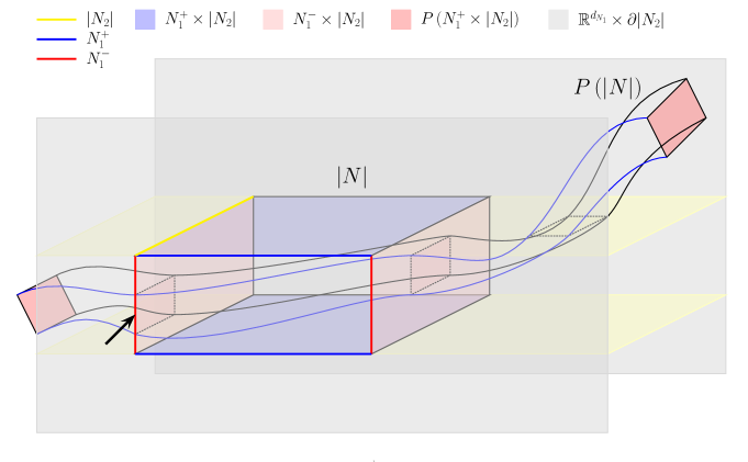
Figure 1: An example of a covering relation $N\stackrel{{\scriptstyle P}}{{\Longrightarrow}}N$ on an h-set with tail $N=(N_{1},|N_{2}|)$, $u_{N_{1}}=1,s_{N_{1}}=1$. The tail $|N_{2}|$ is closed and convex in a potentially infinite dimensional space. The legend is as follows: the set $|N|$ is the parallelepiped in the middle, whereas its image $P(|N|)$ is stretched across $N$. The finite dimensional part is drawn in (x,y)-plane (width and height of the page), where the tail is drawn in z-coordinate (depth). The yellow thick line is one copy of the set $|N_{2}|$ (the tail part), blue thick lines mark the set $N_{1}^{+}$ (the ,,entrance set” of the finite dimensional part of $N$), red thick lines mark the set $N_{1}^{-}$ (the ,,exit set” of the finite dimensional part of $N$), light-blue and light-red polygons mark the entrance set $N_{1}^{+}\times|N_{2}|$ and the exit set $N_{1}^{-}\times|N_{2}|$, respectively. The grey planes denote the boundary of the strip $\mathbb{R}^{d_{N_{1}}}\times|N_{2}|$ - the image of $|N|$ under $P$ is forbidden to extend beyond those planes in z-coordinate due to the condition (C0). The set $P(|N|)$ does not ,,touch” the entrance set $N_{1}^{+}\times|N_{2}|$ - condition (C3) and the exit set $N_{1}^{+}\times|N_{2}|$ is mapped outside $|N|$ (red polytopes on left and right part of the picture) - condition (C2). Please note, that the image $P(|N|)$ is allowed to touch the boundary $N_{1}\times\operatorname{\partial}|N_{2}|$ (place marked with a black arrow) as long as it does not go beyond the grey planes. It is also allowed to bend in the stable direction of the finite dimensional part outside the strip bounded by yellow hyperplanes (see right part of the picture). It is easy to see, that the map $P$ can be homotopied, with a straight line homotopy fulfilling condition (C0), to a map $(x,y,r)\mapsto(2\cdot x,0,\bar{r})$, where $\bar{r}\in|N_{2}|$ (up to the coordinate change $c_{N}$) - condition (C4).

Now we will state theorems, similar to Theorem 23, that joins the sequences of covering relations to the real dynamics happening in the underlying compact maps. We start with definitions:

Definition 11

Let $k>0$ be fixed integer and let $B$ be a transition matrix: $B\in\mathcal{M}(k,k)$ such that $\operatorname{\mathbf{B}}_{ij}\in\{0,1\}$. Then define:

$$\Sigma^{+}_{B}=\left\{s\in\{1,\ldots,k\}^{\mathbb{N}}:\operatorname{\mathbf{B}}_{s_{i},s_{i+1}}=1,\quad\forall i\in\mathbb{N}\right\}$$

and a shift function $\sigma:\Sigma^{+}_{B}\to\Sigma^{+}_{B}$ by

$$\sigma(s)_{i}=s_{i+1}.$$

The pair $(\Sigma^{+}_{B},\sigma)$ is called a subshift of finite type with transition matrix $B$.

Definition 12

Let $\mathcal{F}$ be a family of compact maps in a real Banach space $\mathcal{X}$.

We say that $\Gamma=(\mathcal{N},\mathcal{F},Cov)$ is a set of covering relations on $\mathcal{X}$ iff

• $\mathcal{F}$ is a collection of continuous and compact maps on $\mathcal{X}$,

• $\mathcal{N}$ is a collection of h-sets with tails $N_{i}\subset\mathcal{X}$, $i\in\{1,..,k\}$,

• $Cov\subset\mathcal{N}\times\mathcal{F}\times\mathcal{N}$ is a collection of covering relations, that is if $(N_{i},P_{l},N_{j})\in Cov$ then $N_{j}\stackrel{{\scriptstyle P_{l}}}{{\Longrightarrow}}N_{j}$.

A transition matrix $B\in\mathcal{M}(k,k)$ associated to $\Gamma$ is defined as:

$$B_{ij}=\begin{cases}1&\textrm{if there exists covering relation }N_{i}\stackrel{{\scriptstyle P_{l}}}{{\Longrightarrow}}N_{j}\in Cov\\ 0&\textrm{otherwise}.\end{cases}$$ (44)

Definition 13

A sequence $(x_{i})_{i\in\mathbb{N}}$ is called a full trajectory with respect to family of maps $\mathcal{F}=\{f_{i}:1\leq i\leq m\}$ if for all $i\in\mathbb{N}$ there is $j(i)\in\{1,\ldots,m\}$ such that $f_{j(i)}(x_{i})=x_{i+1}$.

Now we state two main theorems:

Theorem 24

The claim of Theorem 23 is true for a covering relation chain where sets $X_{i}$ are h-sets with tail in a real Banach space $\mathcal{X}$.

Theorem 25

Let $\Gamma=(\mathcal{N},\mathcal{F},Cov)$ be a set of covering relations and let $B$ be its transition matrix.

Then, for every sequence of symbols $(\alpha_{i})_{i\in\mathbb{N}}\in\Sigma^{+}_{B}$ there exist $(x_{i})_{i\in\mathbb{N}}$ - a full trajectory with respect to $\mathcal{F}$, such that $x_{i}\in X_{\alpha_{i}}$. Moreover, if $(\alpha_{i})_{i\in\mathbb{N}}$ is $T$-periodic, then the corresponding trajectory may be chosen to be a $T$-periodic sequence too.

Before we do the proofs of Theorems 24 and 25, we note that the examples of results that can be obtained with covering relations on h-sets with tails are the same as given before in Section 4.2 in the case of a finite-dimensional space $\mathbb{R}^{d}$. In the context of DDEs we will use those theorems for h-sets with tails in the form of a (p,n)-fset: $N=(N_{1},|N_{2}|)=X(A,R)\subset C^{n}_{p}$. The natural decomposition is such that $\{\xi\in\left(C([0,h],\mathbb{R}^{d})\right)^{p}:[\xi]\subset R\}=|N_{2}|$ (the tail) and $N_{1}=A\subset\mathbb{R}^{M(d,p,n)}$ (the finite-dimensional part). In each application presented later in the paper we will decide on $u_{N_{1}}$ and on the coordinates $c_{N_{1}}$ on the finite-dimensional part $A$.

Proof of Theorem 24: We proceed in a way, similar to the proof of Theorem 2 in [39]. To focus the attention and get rid of too many subscripts at once, we assume without loss of generality that $c_{X_{i}}=Id$ for all $i$ and $X_{i}=N_{i}\times R_{i}$, where $N_{i}\in\mathbb{R}^{M}$ is the finite-dimensional part.

Let now denote $X=X_{1}\times\ldots\times X_{k}$, $N=N_{1}\times\ldots\ N_{k}$ and $R=R_{1}\times\ldots\ R_{k}$. Let also denote by $\mathcal{Y}=\mathbb{R}^{M\cdot k}\times R$. With a slight abuse of notation we can write $X\subset\mathcal{Y}$ and that $\mathcal{Y}\subset\mathcal{X}^{k}$. Since $\mathcal{X}^{k}$ is a Banach space (with the product maximum norm) so is $\mathcal{Y}$ with topology inherited from the space $\mathcal{X}^{k}$. Moreover, we have $X\subset\mathcal{Y}$ with $\operatorname{int}_{\mathcal{Y}}X=\operatorname{int}N_{1}\times R_{1}\times\ldots\times\operatorname{int}N_{k}\times R_{k}$. This will be important for proving that a fixed point problem we are going to construct is solution-free on the boundary of $X$ in $\mathcal{Y}$.

We construct zero finding problem:

$$\begin{array}[]{rcl}P_{k}(x_{k})&=&x_{1}\\ P_{1}(x_{1})&=&x_{2}\\ &\cdots&\\ P_{k-1}(x_{k-1})&=&x_{k},\\ \end{array}$$ (45)

and we denote the left side of (45) by $F(x)$ and we are looking for a solution $x=F(x)$ with $x=(x_{1},x_{2},\ldots,x_{k})\in X$. With the already mentioned abuse of notation, we can write $F(a,\xi)=(b,\zeta)$ for $a\in\mathbb{R}^{M\cdot k}$, $\xi\in R$. In a similar way we construct a homotopy $H$, by pasting together homotopies from the definition of h-sets with tails $X_{i}$:

$$H(t,x)=\left(H_{k}\left(t,x_{k}\right),H_{1}\left(t,x_{1}\right),\ldots,H_{k-1}\left(t,x_{k-1}\right)\right)$$

It is obvious that $H(0,\cdot)=F$ and we will show that $H(t,\cdot)$ is fixed point free (admissible) on the boundary $\operatorname{\partial}_{\mathcal{Y}}X$. Indeed, since $\operatorname{int}_{\mathcal{Y}}X=\operatorname{int}N_{1}\times R_{1}\times\ldots\times\operatorname{int}N_{k}\times R_{k}$ then for $(b,\zeta)\in\operatorname{\partial}_{\mathcal{Y}}X$ there must be $i\in\{1,\ldots,k\}$ such that $b_{i}\in\operatorname{\partial}N_{i}=N_{i}^{+}\cup N_{i}^{-}$. If $b_{i}\in N_{i}^{-}$ then (C2) gives $H_{i}\left(t,(b_{i},\zeta_{i})\right)\notin X_{i+1}$ and consequently $(\operatorname{\mathbf{B}}_{i+1},\zeta_{i+1})\neq H\left(t,(b,\zeta)\right)_{i+1}$ (note, if $i=k$, the we set $i+1=1$). If $b_{i}\in N_{i}^{+}$, then from (C3) it follows that $H_{i-1}\left(t,(\operatorname{\mathbf{B}}_{i-1},\zeta_{i-1})\right)\notin\left(N_{i}^{+}\times|R_{i}|\right)$ and so $H\left(t,(b,\zeta)\right)_{i}\neq(b_{i},\zeta_{i})$ (note, if $i=1$, the we set $i-1=k$). Therefore $H$ is admissible, $H(t,x)\neq x$ for all $x\in\operatorname{\partial}_{\mathcal{Y}}X$. Of course $H$ is also continuous and compact.

Now, $\mathcal{Y}$ is an ANR (Corollary 4.4 in §11. of [8]) so fixed point index $\iota(H(t,\cdot),X)$ is well defined and constant for all $t\in[0,1]$. Applying Multiplicativity, Normalization (on the tail part) and 21 on $H(1,\cdot)$ we get $\iota(H(1,\cdot),X)=\Pi\iota\left(A_{i},B^{u}(0,1)\right)=\pm 1$ (since $det(Id-A_{i})\neq 0$ as $\|A_{i}\|>1$ due to (C4)).

Finally, Existence property yields a fixed point $\bar{x}$ to $H(0,x)=F(x)=x$.  

Proof of Theorem 25 is almost the same as of Theorem 3 in [39], with the exception that the sets $X_{i}$ are not compact. This is overcome by considering the convergence of sequences of points in the images $P_{i}(X_{i})$, which are pre-compact by the assumption on $P_{i}$’s.  

We conclude with a lemma that allows to easily check whether $N\stackrel{{\scriptstyle P}}{{\Longrightarrow}}M$ in case $u_{N}=u_{M}=1$. We will check the assumptions of this lemma later in Section 5, with the help of a computer.

Lemma 26

For a h-set with tail $N$ let define:

• $N_{c}^{l}=\{-1\}\times\operatorname{\mathbf{B}}_{s}\times|N|$, $N^{l}=c_{N}^{-1}(N_{c}^{l})$ - the left edge of $N$, and

• $N_{c}^{r}=\{1\}\times\operatorname{\mathbf{B}}_{s}\times|N|$, $N^{r}=c_{N}^{-1}(N_{c}^{r})$ - the right edge of $N$.

Let $\mathcal{X}$ be a Banach space, $X\subset\mathcal{X}$ be an ANR, $N=(N_{1},|N_{2}|)$, $M(M_{1},|M_{2}|)$ be h-sets with tails in $X$ with $u_{N}=u_{M}=1$ and $P:|N|\to X$ be a continuous and compact map such that the following conditions apply (with $P_{c}=c_{M}\circ P\circ c_{N}^{-1}:N_{c}\to M_{c}$):

1. (CC1) $\pi_{\mathcal{X}_{2}}P\left(|N|\right)\subset|M_{2}|$;

2. Either (CC2A)

   $$P_{c}\left(N_{c}^{l}\right)\subset(-\infty,-1)\times\mathbb{R}_{s}\times|M_{2}| and P_{c}\left(N_{c}^{r}\right)\subset(1,\infty)\times\mathbb{R}_{s}\times|M_{2}|$$

   or (CC2B)

   $$P_{c}\left(N_{c}^{l}\right)\subset(1,\infty)\times\mathbb{R}_{s}\times|M_{2}| and P_{c}\left(N_{c}^{r}\right)\subset(-\infty,-1)\times\mathbb{R}_{s}\times|M_{2}|$$

3. (CC3) $P_{c}\left(N_{c}\right)\cap\left(\operatorname{\mathbf{B}}_{s}\times|M_{2}|\right)=\emptyset$

Then $N\stackrel{{\scriptstyle P}}{{\Longrightarrow}}M$ with the homotopy given as $H(t,\cdot)=(1-t)\cdot P+t\cdot(A,0,\bar{r})$, where $A:\mathbb{R}\to\mathbb{R}$ such that $Ax=2x$ (CC2A) or $Ax=-2x$ (CC2B) and $\bar{r}$ is any selected point in $|M_{2}|$.

Proof: (C0) and (C1) from Definition 10 are obviously satisfied. We also have (CC2) implies (C2) and (CC3) is the same as (C3). Therefore, we only need to show (C4), that is, the image of the homotopy computed on the set $\operatorname{\partial}\operatorname{\mathbf{B}}_{u}\times\overline{\operatorname{\mathbf{B}}_{s}}\times|N_{2}|$ does not touch the set $M_{c}$. This is obvious from the definition of $A$ in both cases (CC2A) and (CC2B).  

Figure 1 presents such a covering in case $u=s=1$ and $N=M$. The easiest way to assure (CC1) and (CC3) is to assume $P_{c}(N_{c})\subset\mathbb{R}\times\operatorname{\mathbf{B}}_{s}\times|M_{2}|$ - in fact we check this in our computer assisted proofs presented in the next section.

5 Applications

In this section we present applications of the discussed algorithm to two exemplary problems. First one is a computer assisted proof of symbolic dynamics in a delay-perturbed Rössler system [28]. The proof is done for two different choices of perturbations. The second application consists of proofs of (apparently) unstable periodic orbits in the Mackey-Glass equation for parameter values for which Mackey and Glass observed chaos in their seminal paper [23].

Before we state the theorems, we would like to discuss presentation of floating point numbers in the article. Due to the very nature of the implementation of real numbers in current computers, numbers like $0.1$ are not representable [29], i.e. cannot be stored in memory exactly. On the other hand, many numbers representable on the computer could not be presented in the text of the manuscript in a reasonable way, unless we adopt not so convenient digital base-2 number representation. However, the implementation IEEE-754 of the floating point numbers on computers [29] guarantees that, for any real number $x$ and its representation $\tilde{x}$ in a computer format, there is always a number $|\varepsilon|\leq\varepsilon_{machine}$ such that $\tilde{x}=x(1+\varepsilon)$. The number $\varepsilon_{machine}$ defines the machine precision, and, for the double precision C++ floating-point numbers that we use in the applications, it is of the order $10^{-16}$. Finally, in our computations we use the interval arithmetic to produce rigorous estimates on the results of all basic operations such as $+$, $-$, $\times$, $\div$, etc. In principle, we operate on intervals $[a,b]$, where $a$ and $b$ are representable numbers, and the result of an operation contains all possible results, adjusting end points so that they are again representable numbers (for a broader discussion on this topic, see the work [34] and references therein). For a number $x\in\mathbb{R}$ we will write $[x]$ to denote the interval containing $x$. If $x\in\mathbb{Z}$ then we have $[z]=[z,z]$, as integer numbers (of reasonably big value) are representable in floating point arithmetic.

Taking all that into account we use the following convention:

• whenever there is an explicit decimal fraction defined in the text of the manuscript of the form $d_{1}d_{2}\cdots d_{k}.q_{1}q_{2}\cdots q_{m}$ then that number appears in the computer implementation as

  $$[d_{1}d_{2}\cdots d_{k}q_{1}q_{2}\cdots q_{k}]\div[10^{m}],$$

  where $\div$ is computed rigorously with the interval arithmetic. For example, number $10^{-3}=0.001$ appears in source codes as Interval(1.) / Interval(1000.).

• whenever we present a result from the output of the computer program $x$ as a decimal number with non-zero fraction part, then we have in mind the fact that this represents some other number $y$ - the true value, such that $y=x(1+\varepsilon)$ with $|\varepsilon|\leq\varepsilon_{machine}$. This convention applies also to intervals: if we write interval $[a_{1},a_{2}]$, then there are some representable computer numbers $b_{1}$, $b_{2}$ which are true output of the program, so that $b_{i}=a_{i}(1+\varepsilon_{i})$.

• if we write a number in the following manner: $d_{1}.d_{2}\cdots d_{k}{}^{u_{1}u_{2}\cdots u_{m}}_{l_{1}l_{2}\cdots l_{m}}$ with digits $l_{i},u_{i},d_{i}\in\{0,..,9\}$ then it represents the following interval

  $$\left[d_{1}.d_{2}\cdots d_{k}l_{1}l_{2}\cdots l_{m},d_{1}.d_{2}\cdots d_{k}u_{1}u_{2}\cdots u_{m}\right].$$

  For example $12.3_{456}^{789}$ represents the interval $[12.3456,12.3789]$ (here we also understand the numbers taking into account the first two conventions).

The last comment concerns the choice of various parameters for the proof, namely, the parameters of the space $C^{n}_{p}$ and the initial sets around the numerically found approximations of the dynamical phenomena under consideration. The later strongly depends on the investigated phenomena, so we will discuss general strategy in each of the following sections, whereas the technical details are presented in Appendices A and B.

The choice of parameters $n$ and $p$ corresponds basically to the choice of the order of the numerical method and a fixed step size $h=\frac{\tau}{p}$, respectively.

Usually, in computer assisted proofs, we want $n$ to be high, so that the local errors are very small. In the usual case of ODEs with $f\in C^{\infty}$ we can use almost any order, and it is easy for example to set $n=40$. However, in the context of $C^{n}_{p}$ spaces and constructing Poincaré maps for DDEs, we are constrained with the long enough time $T=(n+1)\cdot\tau$ (Definition 3) to obtain well defined maps. Therefore, the choice of $n$ corresponds usually to the return time to section $t_{P}$ for a given Poincaré map, satisfying $t_{P}(X_{0})>(n+1)\cdot\tau$, for some set of initial data $X_{0}\subset C^{n}_{p}$.

The choice of the step size $h$ is more involved. It should not be too small, to reduce the computational time and cumulative impact of all local errors after many iterations, and not so big, as to effectively reduce the size of the local error. Also, the dynamics of the system (e.g. stiff systems) can impact the size of the step size $h$. In the standard ODE setting, there are strategies to set the step size dynamically, from step to step, e.g. [9], but in the setting of our algorithm for DDEs, due to the continuity issues described in Section 3, we must stick to the fixed step size $h=\frac{\tau}{p}$. The step size must be also smaller than the (apparent) radius of convergence of the forward Taylor representation of the solution at each subinterval, but this is rarely an issue in comparison to other factors, e.g. the local error estimates. In our applications we chose $p=2^{m}$ for a fixed $m\in\mathbb{N}$, so that the grid points are representable floating point numbers (but the implementation can work for any $p$).

We also need to account for the memory and computing power resources. For $d$-dimensional systems (2), and with $n$, $p$ fixed, we have that the representation of a Lohner-type set $A=x_{0}+C\cdot r_{0}+E$ in phase-space of $\varphi$, where $C\in\mathcal{M}{M,M}$, requires at least $O(M^{2})$, with $M=O(d\cdot n\cdot p)$. Then, doing one step of the full step algorithm is of $O(d^{2}\cdot n^{2}\cdot M)$ computational complexity. Due to the long enough time integration, computation of a single orbit takes usually $O(n\cdot p)$ steps, and we get the computational complexity of computing image $P(X)$ for a single set $X$ of $O(d\cdot n^{2}\cdot d\cdot p\cdot n\cdot M)=O(d\cdot n^{2}\cdot M\cdot M)=O(M^{2})$ (if we assume $n,d<<M$). Therefore, we want to keep $M^{2}=(d\cdot n\cdot p)^{2}$ of reasonable size, both because of time and memory constraints. Our choice here is $M\leq 10^{3}$.

5.1 Symbolic dynamics in a delay-perturbed Rössler system

In the first application, we use Rössler ODE of the form [28]:

$$x^{\prime} = -(y+z)$$

$$y^{\prime} = x+ay$$ (46)

$$z^{\prime} = b+z(x-c).$$ (47)

In what follows we will denote r.h.s. of (46) by $f$ and by $v\in\mathbb{R}^{3}$ we denote vector $v=(x,y,z)$. By $\pi_{x}$ we denote projection onto $x$ coordinate, similarly for $\pi_{y},\pi_{z}$.

We set the classical value of parameters $a=b=0.2$, $c=5.7$ [28]. For those parameter values, an evidence of a strange attractor was first observed numerically in [28] , see Fig. 2. In [42], it was proved by computer assisted argument that there is a subset of the attractor which exhibit symbolic dynamics. A more recent results for Rössler system can also be found in [6] (Sharkovskii’s theorem) and the methodologies there should be easily adaptable in the context of delay perturbed systems presented in this paper.

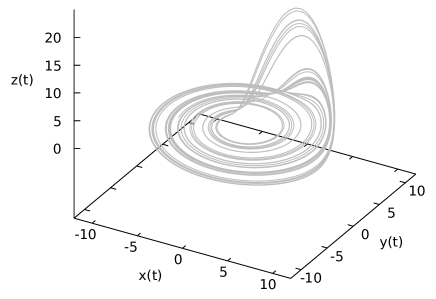
Figure 2: Numerically observed attractor in the Rössler ODE for classical values of parameters: $a=b=0.2$, $c=5.7$. Picture generated by integrating forward in time single trajectory for a long time.

We are going to study a delayed perturbation of the Rössler system (46) of the following form:

$$v^{\prime}(t)=f(v(t))+\epsilon\cdot g(v(t-1)),$$ (48)

where parameter $\epsilon$ is small. We consider two toy examples: first, where $g=f$ and the second one where $g$ is given explicitly as

$$g(x,y,z)=\left(\sin(x\cdot y),\sin(y\cdot z),\sin(x\cdot z)\right).$$ (49)

We expect that for any bounded $g$ there should be a sufficiently small $\epsilon$ [33] so that the dynamics of the perturbed system is preserved. However, in this work, we study explicitly given value for $\epsilon$.

Remark 27

The source codes of the proof are generic. The interested reader can experiment with other forms of the perturbation by just changing the definition of the function $g$ in the source codes of the example.

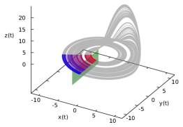
Figure 3: The numerically observed attractors for the system studied in Theorem 28. The cases (a)-(c) are shown from left to right, respectively. The grey attractor is the very long trajectory $v(t)$ obtained for a single constant initial function. The section $S_{0}$, represented as a green rectangle on the picture, spans in fact across the space $\mathbb{R}^{3}$, as can bee seen by the red to blue region that shows the segments of $v$ which lie on the section $S_{0}$, i.e. the set $\{v_{t}:\pi_{x}(v(t))=0\}$. The colours are assigned with ascending $\pi_{y}v(t)$ value. Those segments are used to define the $W_{u}$ coordinate in the set $X(A,\Xi)$.

We will be studying the properties of a Poincaré map defined on the section $S_{0}\subset C^{n}_{p}$ given by:

$$S_{0}=\{v\in C^{n}_{p}:\pi_{x}(v(0))=0\}.$$

The section $S_{0}$ in an extension to $C^{n}_{p}$ of the section $S=\{v\in\mathbb{R}^{3}:\pi_{x}v=0\}\subset\mathbb{R}^{3}$ used in the proofs in [42]. The section $S$ is drawn in green in Fig 3, whereas the projection of the attractor onto section $S_{0}$ is drawn as a blue-red gradient (the solution segments $v$ with $\pi_{x}v(0)=0$).

In what follows, we set the parameters for the space $C^{n}_{p}$ to $p=32$ and $n=3$. We prove, with the computer assistance, the following theorems:

Theorem 28

For parameter values $a=b=0.2$, $c=5.7$ in (46) there exists sets $X_{A}=X(A,\Xi),X_{1}=X(N_{1},\Xi),X_{2}=X(N_{2},\Xi)\subset S_{0}$ with explicitly given $A,N_{1},N_{2}$ and $\Xi$, such that for the system (48) with $\epsilon=10^{-3}$ and perturbations: (a) $g\equiv 0$ - original system treated as a DDE, (b) $g=f$ and (c) $g$ given as in in Eq (49) we have the following:

1. $P(X(A,\Xi))\subset X(A,\Xi)$ and, in consequence, there exists a non-empty invariant set in $X(A,\Xi)$ for the map $P:S_{0}\to S_{0}$.

2. the invariant set $I=Inv(P^{2},X_{1}\cup X_{2})$ of $X_{1}\cup X_{2}$ under the map $P^{2}$ on $I$ is non-empty and the dynamics of $P^{2}$ is conjugated to the shift on two symbols ($\sigma:\Sigma_{2}\to\Sigma_{2}$, $\sigma(e_{k})=e_{k+1}$), i.e. if we denote by $g:I\to\Sigma_{2}$ the function $g(x)_{k}=i\iff P^{2k}(x)\in X_{i}$, then we have $g\circ P^{2}|_{I}=\sigma\circ g$.

Before we present the proof(s), we would like to make a remark on the presentation of the data from the computer assisted part:

Remark 29 (Convention used in the proofs)

The proofs of those theorems are computer assisted and the parameters of the phase-space $C^{n}_{p}$ of representations are $d=3$, $p=32$, $n=3$, giving in total the dimension of the finite dimensional part of $M(d,p,n)=d\cdot(1+p\cdot(n+1))=387$. Therefore it is not convenient to present complete data of the proofs in the manuscript. Instead, we assume the sets are explicitly given in the following forms (and the interested reader is refereed to Appendix B for the details on how they are constructed):

$$X_{A}=X(A,R):\quad A=v_{ref}+C\cdot\{0\}\times W_{u}\times\operatorname{\mathbf{B}}^{\|\cdot\|_{\infty}}_{M-2}(0,1)$$

$$X_{i}=X(N_{i},R):\quad N_{i}=v_{ref}+C\cdot\{0\}\times W_{i}\times\operatorname{\mathbf{B}}^{\|\cdot\|_{\infty}}_{M-2}(0,1)$$

$$\Xi=\operatorname{\mathbf{B}}^{\|\cdot\|_{\infty}}_{d\cdot p}(0,1)\quad$$

with $v_{ref}\in S_{0}$, $W_{u},W_{1},W_{2}$ closed intervals such that $W_{1}\cap W_{2}=\emptyset$ and $W_{i}\subset W_{u}\subset\mathbb{R}$, and we remind $\operatorname{\mathbf{B}}^{\|\cdot\|_{\infty}}_{D}(0,1)$ denotes the unit radius ball in the $\max$ norm in $\mathbb{R}^{D}$ centred at $0$. Note, this description of sets makes it clear they are h-sets with tails on $S_{0}$ (up to the scaling of nominally unstable direction $W$), where $u=1$ and $s_{A}=s_{N_{i}}=s=M(d,p,n)-2$, the support set $|A|=\{0\}\times W_{u}\times\operatorname{\mathbf{B}}^{\|\cdot\|_{\infty}}_{M-2}(0,1)$ and the affine coordinate change $c_{A}(\cdot)=v_{ref}+C(\cdot)$ with inverse change $c_{A}^{-1}(\cdot)=C^{-1}(\cdot-v_{ref})$. Now, the computation of any Poincaré map $P:X_{A}\to S_{0}$ for the initial data $X(A,\Xi)$ produces set $X(B,\Omega)=P(X(A,\Xi))$ and there exist sets

$$c_{A}^{-1}(B) =\ B_{c} \subset\ \{0\}\times(B_{c})_{2}\times\operatorname{\mathbf{B}}^{\|\cdot\|_{\infty}}_{M-2}(0,r_{B})$$

$$\ \Omega \subset\ \operatorname{\mathbf{B}}^{\|\cdot\|_{\infty}}_{d\cdot p}(0,r_{\Omega})$$

for some $r_{B},r_{\Omega}\in\mathbb{R}_{+}$. This allows to describe the geometry of $X(A,\Xi)$ and (estimates on) $P(X(A,\Xi))$ by just a couple of numbers: $W_{u}$, $\pi_{2}B_{c}$ (the size of set $B$ in the nominally unstable direction), $r_{B}$ (upper bound on all coefficients in the finite nominally stable part) and $r_{\Omega}$ (upper bound on all $\xi$ in the tail part), which are suitable for a concise presentation in the manuscript.

The sets used in the computations are obtained by computing the appropriately enlarged enclosure on the set of segments of solutions to the unperturbed ODE (46). We choose a set $\tilde{A}\subset\mathbb{R}^{3}$ such that $\tilde{A}\in\{v\in\mathbb{R}^{3}\pi_{x}v=0\}$ is a trapping region for the Poincaré map of the unperturbed ODE: $P(\tilde{A})\subset\tilde{A}$. Then we choose a set $X(A,\Xi)$ to contain the segments of $\tilde{A}$ propagated back in time for a full delay with the unperturbed ODE:

$$\left\{v:[-1,0]\to\mathbb{R}:v(0)\in A,v(s)=\varphi_{0}(s,v(0))\right\}\subset A,$$

where $\varphi_{0}$ is the flow in $\mathbb{R}^{3}$ for (46). Detailed procedure how the set $A$ was generated is described in the Appendix B. The set $\tilde{A}$ was chosen to be $\{0\}\times[-10.7,-2.2]\times[0.021,0.041]$, whereas the sets $\tilde{N}_{1}=[-8.4,-7.6]$ and $\tilde{N}_{2}=[-5.7,-4.6]$. Finally, the orbit $v_{0}$ with $\pi_{2}v_{0}(0)=-6.8$ is selected among the orbits in the attractor as the reference point of the sets $X_{A},X_{1},X_{2}$. The set $W_{u}$ is chosen as $W_{u}=\pi_{2}A_{c}=\pi_{y}\tilde{A}-\pi_{2}v_{0}(0)=[-3.9,4.6]$. The same is true for sets $N_{1},N_{2}$, with $W_{1}=[-1.6,-0.8]$, $W_{2}=[1.1,2.2]$.

Now we can proceed to the proofs.

Proof o Theorem 28 The proofs for parts (a), (b), and (c) follow the same methodology, therefore we present the details only for case (a) and then, only the estimates from the other two cases. In principle, we will show that $P(X_{A})\subset X_{A}$ and $X_{i}\stackrel{{\scriptstyle P^{2}}}{{\Longrightarrow}}X_{j}$ for all $i,j\in\{1,2\}$ and then apply Theorem 25.

The set $X(A,R)$ and two other sets are given as described in Remark 29. The computer programs for the proof are stored in ./examples/rossler_delay_zero. The data for which presented values were computed is stored in ./data/rossler_chaos/epsi_0.001. See Appendix B for more information. Additionally to the estimates presented below, the computer programs verify that $t_{P}(x)>(n+1)$ (i.e. long enough for Poincaré maps to be well defined) and that the function $t_{P}(\cdot)$ is well defined. For details, see the previous work [34].

First, we prove that $P_{c}(X(A,\Xi))\subset(A_{c},\Xi)$. Let $(B_{c},\Omega)$ will be output of the rigorous program rig_prove_trapping_region_exists run for the system in case (a) such that $P_{c}(X(A,\Xi))\subset(B_{c},\Omega)$. It suffices to show the following:

• $\pi_{2}P_{c}(X(A,\Xi))=\pi_{2}B_{c}\subset W_{u}=\pi_{2}A_{c}$;

• $\pi_{i}P_{c}(X(A,\Xi))=\pi_{i}B_{c}<1$ for all $i>2$;

• $\pi_{\Xi_{i}}P_{c}(X(A,\Xi))=\pi_{i}\Omega<1$ for all $i\in\{1,\ldots,p\cdot d\}$.

Indeed, we have:

• $\pi_{2}P_{c}(X(A,\Xi))=[-3.786230021035,3.92103823500285]\subset[-3.9,4.6]=W_{u}$;

• $\pi_{i}P_{c}(X(A,\Xi))\leq 0.910355124006778<1$, for $i>2$;

• $\pi_{\Xi_{i}}P_{c}(X(A,\Xi))\leq 0.395102819146026<1$ for all $i$.

Which finishes the proof of the first assertion.

For the second assertion we prove that we have a set of full covering relations:

$$X_{i}\stackrel{{\scriptstyle P^{2}}}{{\Longrightarrow}}X_{j},\quad i,j\in\{1,2\}.$$

We remind that the sets $N_{i,c}=\{0\}\times[W_{i}^{l},W_{i}^{r}]\times\operatorname{\mathbf{B}}^{\|\cdot\|_{\infty}}_{M-2}(0,1)$ with $W_{1}=[-1.6,-0.8]$, $W_{2}=[1.1,2.2]$. The program ./rig_prove_covering_relations produces the following inequalities:

• (L1-L1) $\pi_{2}P^{2}_{c}(X(N_{1}^{l},\Xi))=-1._{696238902429803}^{708946819732338}<-1.6=\pi_{2}N_{1,c}^{l}<\pi_{2}N_{2,c}^{l}$

• (R1-R2) $\pi_{2}P^{2}_{c}(X(N_{1}^{r},\Xi))=2.4_{09511664184434}^{17718805618395}>2.2=\pi_{2}N_{2,c}^{r}>\pi_{2}N_{1,c}^{r}$

• (R2-L1) $\pi_{2}P^{2}_{c}(X(N_{2}^{r},\Xi))=-1.83_{8887194518363}^{9215629292839}<-1.6=\pi_{2}N_{1,c}^{l}<\pi_{2}N_{2,c}^{l}$

• (L2-R2) $\pi_{2}P^{2}_{c}(X(N_{2}^{l},\Xi))=2.2_{69015891346912}^{70120359885664}>2.2=\pi_{2}N_{2,c}^{r}>\pi_{2}N_{1,c}^{l}$,

where sets $N^{l}$, $N^{r}$ etc. are defined as in Lemma 26. It is ease to see that, those inequalities, together with the existence of trapping region $X_{A}$, imply that for each $i,j\in\{1,2\}$ conditions (CC1)-(CC3) in Lemma 26 are satisfied, that is $X_{i}\stackrel{{\scriptstyle P^{2}}}{{\Longrightarrow}}X_{j}$, which finishes the proof for the case (a) after applying Theorem 25.

For the cases (b) and (c) we only present estimates:

• Case (b), $g=f$. Output from rig_prove_trapping_region_exists is:

  • $\pi_{2}P_{c}(X(A,\Xi))=[-3.82791635121864,3.90123013871349]\subset[-3.9,4.6]=W_{u}$;

  • $\pi_{i}P_{c}(X(A,\Xi))\leq 0.960537051554584<1$, for $i>2$;

  • $\pi_{\Xi_{i}}P_{c}(X(A,\Xi))\leq 0.397264977921163<1=r_{\Xi}$, for all $i$.

  Output from program ./rig_prove_covering_relations is:

  • (L1-L1) $\pi_{2}P^{2}_{c}(X(N_{1}^{l},\Xi))=-1.6_{68486957556001}^{84410417326001}<-1.6=\pi_{2}N_{1,c}^{l}<\pi_{2}N_{2,c}^{l}$

  • (R1-R2) $\pi_{2}P^{2}_{c}(X(N_{1}^{r},\Xi))=2.4_{64065036803807}^{74268236696726}>2.2=\pi_{2}N_{2,c}^{r}>\pi_{2}N_{1,c}^{r}$

  • (R2-L1) $\pi_{2}P^{2}_{c}(X(N_{2}^{r},\Xi))=-1.76_{7206286440370}^{9151140189891}<-1.6=\pi_{2}N_{1,c}^{l}<\pi_{2}N_{2,c}^{l}$

  • (L2-R2) $\pi_{2}P^{2}_{c}(X(N_{2}^{l},\Xi))=2.36_{0282881761384}^{2685243092644}>2.2=\pi_{2}N_{2,c}^{r}>\pi_{2}N_{1,c}^{r}$

• Case (c), $g$ as in (49). Output from rig_prove_trapping_region_exists is:

  • $\pi_{2}P_{c}(X(A,\Xi))=[-3.78710970137727,3.92188126709857]\subset[-3.9,4.6]=W_{u}$;

  • $\pi_{i}P_{c}(X(A,\Xi))\leq 0.951680057117636<1$, for $i>2$;

  • $\pi_{\Xi_{i}}P_{c}(X(A,\Xi))\leq 0.459753301095895<1$, for all $i$.

  Output from program ./rig_prove_covering_relations is:

  • (L1-L1) $\pi_{2}P^{2}_{c}(X(N_{1}^{l},\Xi))=-1._{695427259804897}^{714200213156898}<-1.6=\pi_{2}N_{1,c}^{l}<\pi_{2}N_{2,c}^{l}$

  • (R1-R2) $\pi_{2}P^{2}_{c}(X(N_{1}^{r},\Xi))=2.4_{08774107762390}^{20396855111791}>2.2=\pi_{2}N_{2,c}^{r}>\pi_{2}N_{1,c}^{r}$

  • (R2-L1) $\pi_{2}P^{2}_{c}(X(N_{2}^{r},\Xi))=-1.8_{38300180457653}^{41157932729915}<-1.6=\pi_{2}N_{1,c}^{l}<\pi_{2}N_{2,c}^{l}$

  • (L2-R2) $\pi_{2}P^{2}_{c}(X(N_{2}^{l},\Xi))=2.2_{67377344403297}^{70144525622461}>2.2=\pi_{2}N_{2,c}^{r}>\pi_{2}N_{1,c}^{r}$

 

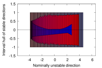
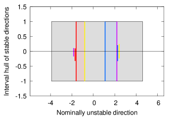
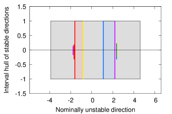
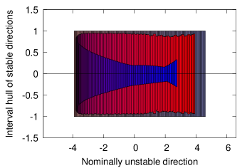
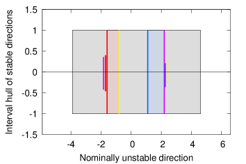
Figure 4: The rigorous estimates obtained in the computer assisted part of the proof of Theorem 28. The cases (a)-(c) are presented top to bottom, respectively. The left picture shows the representation of the computer assisted proof of the trapping region $X_{A}$. The set is divided into 200 pieces $X_{A,i}$ along the $W_{u}$ direction, each piece is coloured according to ascending number. Then for each piece $X_{A,i}$ the image $P(X_{A,i})$ is computed and drawn in the same colour (but with increased intensity). The dimension of the boxes in the $y$ coordinate represents the hull of the nominally stable part of the set $P(X_{A,i})$, i.e. the interval $I_{i}=[y_{lo},y_{up}]$ such that all $\pi_{A_{j}}P_{c}(X)\subset I_{i}$, for $j\in\{3,\ldots,M\}$ and $\pi_{\Xi_{j}}(P_{c}(X))\subset I$ for $j\in\{1,\ldots,p\cdot d\}$. Obviously, each $I_{i}\subset B_{1}\left(0,\max(P(r_{A}),P(r_{\Xi}))\right)$. A clear evidence of the Smale horseshoe-like dynamics can be seen in the picture, as the box is folding on itself under the map $P$. On the right picture one there are represented the sets $X_{1}$ (light red, with red and yellow borders) and $X_{2}$ (light blue, with blue and purple borders). The images of the borders under the map $P^{2}$ are presented as lines (in fact thin boxes) in the grey area outside $X_{1}\cup X_{2}$. It is evident that $P(W_{1,l})$ (red) and $P(W_{2,r})$ (purple) are both mapped to the left of both sets and $P(W_{1,r})$ (yellow) and $P(W_{2,l})$ (blue) are mapped to the right. Therefore condition (CC2A) is satisfied between the sets $X_{1}$ and any of $X_{i}$’s, and condition (CC2B) between $X_{2}$ and any $X_{i}$, $i\in\{1,2\}$. Please consult online version of the plots for better quality.

Fig. 3 shows the numerical representations of the apparent strange attractor in the respective systems, while Fig. 4 depicts the computed estimates of the proof in a human-friendly manner. The total running time of the proof in (a) is around 16 minutes, and the cases (b) and (c) of around 23 minutes. Computations were done on a laptop with Intel® Core^TM i7-10750H 2.60GHz CPU. The majority of the computations is done in the proof of trapping region $X_{A}$, which must be divided into 200 pieces along the vector $W_{u}$. Those computations are easily parallelized (each piece computed in a separate thread). The data and programs used in the proofs are described in more details in Appendix B, together with the links to source codes.

5.2 Unstable periodic orbits in Mackey-Glass equation

In this application we study the following scalar equation:

$$x^{\prime}(t)=-\gamma\cdot x(t)+\beta\cdot\frac{x(t-\tau)}{1+(x(t-\tau))^{n}}.$$ (50)

In the paper [23], the authors shown numerical evidence of chaotic attractor in that system, see Fig. 5a. In their work, Mackey and Glass used the following values of parameters: $\tau=2$, $n=9.65$, $\beta=2$, $\gamma=1$. In our previous work [34] we have shown existence of several (apparently) stable periodic orbit for $n\leq 8$. In this work we show that the new algorithm, together with the fixed point index, can be used to prove more diverse spectrum of results. We prove existence of several (apparently) unstable periodic orbits for the classical values of parameters, for which the chaotic attractor is observed, $\tau=2$, $n=9.65$, $\beta=2$, $\gamma=1$.

Remark 30

In what follows we get rid of the variable delay $\tau$ and we rescale the system to have unit delay by the change of variables: $y(t)=x(\tau\cdot t)$. It is easy to see, that the equation (50) in the new variables becomes:

$$y^{\prime}(t)=\tau\cdot f(y(t),y(t-1)),$$

that is, we can remove parameter $\tau$ by rescaling $\beta$ and $\gamma$ to $\bar{\beta}=\tau\cdot\beta$ and $\bar{\gamma}=\tau\cdot\gamma$.

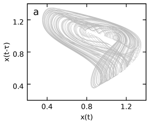
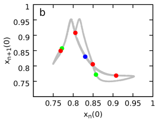
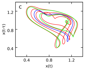
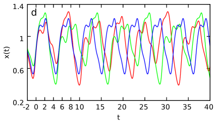
Figure 5: (a) The apparently chaotic attractor of the Mackey-Glass equation (50) for the classical parameter values $\tau=2$, $n=9.65$, $\beta=2$, $\gamma=1$ [23]. The attractor is drawn for a single very long solution, whose time-delay embedding coordinates $(x(t),x(t-\tau))$ are shown in the picture. (b) The representation of the attractor drawn in the coordinates $\left(x_{n}(0),x_{n+1}(0)\right)$, where $x_{n+1}=P(x_{n})$, $x_{n},x_{n+1}\in C([-\tau,0],\mathbb{R})$. The map $P$ is constructed on the section $S=\{x:x(t)=x(t-\tau),x(t)<0.96\}$, see Figure. 13 in [22]. The periodic points $T^{1},T^{2},T^{4}$ of respective periods 1, 2 and 4 for map $P$ are drawn in colors blue, green, red. (c) The same solutions are drawn in the time-delay embedding of the attractor and (d) as the solutions over time long enough to contain basic periods of all presented solutions.

We state the following:

Theorem 31

Each of the three approximate solutions $\bar{T}^{i}$ shown in Figure 5(c)-(d) has a small, explicitly given vicinity $V_{i}\subset C^{n}_{p}$ with $n=4$ and $p=128$ of the initial segment $\bar{T}^{i}_{0}$ such that there exists a true periodic solution $T^{i}$ with the initial segment $T^{i}_{0}\in V_{i}$ of the Mackey-Glass equation (50) for the classical parameter values $\tau=2$, $n=9.65$, $\beta=2$, $\gamma=1$ [23].

Proof of Theorem 31: we use the parameters $\beta=4$ and $\gamma=2$, $n=9.65$ and $\tau=1$ in (50) and we use Remark 30. The proof is similar to that of Theorem 28 and boils down to checking appropriate covering relations. The initial segments $\bar{T}^{i}$ lie on the section $S=\left\{x\in C([0,1],\mathbb{R}):x(0)=x(-1),x(t)<0.96\right\}$. The index $i$ corresponds to the basic period of the solution $T^{i}$ as a periodic point of a map $P:S\to S$. In the coverings we use map $P^{2}$ to guarantee that the return time $t_{P}$ to the section is long enough.

Each of the $V_{i}=X(N_{i},\Xi_{i})$ is given with $N_{i}=\bar{T}^{i}_{0}+C_{i}\cdot r_{i}$ with $r_{i}=\{0\}\times W_{i}^{u}\times[-1,1]^{M-2}$. Additionaly, in case of $T^{4}$ we have another set $V^{\prime}_{4}=X(N^{\prime}_{4},\Xi^{\prime}_{4})$ with $N^{\prime}_{4}$ of the similar form: $N^{\prime}_{4}=P^{2}(\bar{T}^{4})+C^{\prime}_{4}\cdot r^{\prime}_{4}$. In other words, the origin point of the set $N^{\prime}_{4}$ is the second iteration of the Poincaré map $P^{2}$ of the initial segment of $T^{4}$. The sets are obtained as described in Appendix B. Each of these sets define a section $S_{i}=\{x\in C^{n}_{p}:c_{i}\cdot(a(x)-\bar{T}^{i}_{0})=0\}$ (different from $S$), where $c_{i}=(C_{i})_{\cdot,1}$ - the first column of the matrix $C_{i}$. The reason for that is described in the Appendix B, and boils down to assure that $\operatorname{\mathbf{diam}}(t_{P}(X_{i}))$ is as small as possible.

We will show that:

$$V_{1}\stackrel{{\scriptstyle P_{S_{1}\to S_{1}}}}{{\Longrightarrow}}V_{1},\quad\quad\quad V_{2}\stackrel{{\scriptstyle P_{S_{2}\to S_{2}}}}{{\Longrightarrow}}V_{2},\quad\quad\quad V_{4}\stackrel{{\scriptstyle P_{S_{4}\to S^{\prime}_{4}}}}{{\Longrightarrow}}V^{\prime}_{4}\stackrel{{\scriptstyle P_{S^{\prime}_{4}\to S_{4}}}}{{\Longrightarrow}}V_{4},$$ (51)

where the Poincaré maps $P_{S_{i}\to S_{j}}$ are derived from the flow of Eq. (50) and maps indicated sections: $P_{S_{i}\to S_{j}}:S_{i}\to S_{j}$, with additional assumption that the return time $t_{P}$ is long enough. We will drop the subscripts if they are easily known from the context.

For $T^{1}$ we have:

• for all $i>2$, $\left|\pi_{i}P_{c}(X(N_{1},\Xi_{i}))\right|=0.614451801967851<1$

• for all $i$, $\left|\pi_{\Xi_{i}}P_{c}(X(N_{1},\Xi_{i}))\right|=0.999998174289212<1$

• $\pi_{2}P_{c}(X(N_{1}^{r},\Xi))=-{}_{3.845940820239275}^{4.514877050431105}<-1=\pi_{2}N_{c}^{l}$

• $\pi_{2}P_{c}(X(N_{1}^{r},\Xi))={}_{3.827847664967472}^{4.496773405715568}>1=\pi_{2}N_{c}^{r}$

For $T^{2}$ we have:

• for all $i>2$, $\left|\pi_{i}P_{c}(X(N_{2},\Xi_{2}))\right|\leq 0.731193331043839<1$

• for all $i$, $\left|\pi_{\Xi_{i}}P_{c}(X(N_{2},\Xi_{2}))\right|\leq 0.999996951451891<1$

• $\pi_{2}P_{c}(X(N_{2}^{r},\Xi_{2}))={}_{3.995778903452447}^{5.033339010859840}>1=\pi_{2}N_{2,c}^{r}$

• $\pi_{2}P_{c}(X(N_{2}^{r},\Xi_{2}))=-{}_{3.978765934264806}^{5.016322912452834}<-1=\pi_{2}N_{2,c}^{l}$

For $T_{4}$ we have:

• for all $i>2$, $\left|\pi_{i}P_{c}(X(N_{4},\Xi_{4}))\right|\leq 0.999948121260377<1$

• for all $i$, $\left|\pi_{\Xi_{i}}P_{c}(X(N_{4},\Xi_{4}))\right|\leq 0.956276660970399<1$

• $\pi_{2}P_{c}(X(N_{4}^{l},\Xi_{4}))=-{}_{1.1221122505976317}^{3.2368193002087367}<-1={N^{\prime}_{4}}^{l}_{c}$

• $\pi_{2}P_{c}(X(N_{4}^{r},\Xi_{4}))={}_{1.1239689716822263}^{3.2385726261859316}>1={N^{\prime}_{4}}^{r}_{c}$

and

• for all $i>2$, $\left|\pi_{i}P_{c}(X(N^{\prime}_{4},\Xi^{\prime}_{4}))\right|\leq 0.898580326387734<1$

• for all $i$, $\left|\pi_{\Xi_{i}}P_{c}(X(N^{\prime}_{4},\Xi^{\prime}_{4}))\right|\leq 0.952378028038733<1$

• $\pi_{2}P_{c}(X({N^{\prime}_{4}}^{l},\Xi^{\prime}_{4}))={}_{1.6331410212899785}^{3.0485204456349866}>1={N_{4}}^{r}_{c}$

• $\pi_{2}P_{c}(X({N^{\prime}_{4}}^{r},\Xi^{\prime}_{4}))=-{}_{1.6341550945779965}^{3.0495636957165507}<-1={N_{4}}^{l}_{c}$

All those inequalities satisfy appropriate assumptions of Lemma 26. Therefore all the coverings from (51) exist and, from Theorem 25, we infer existence of appropriate periodic points $T^{i}_{0}\in V_{i}$.  

	$L_{\infty}$	$L_{2}$	$H_{4}$	T (expressed in $\tau$)
$T^{1}_{0}$	$2.74231097479455\cdot 10^{-7}$	$3.10483831050838\cdot 10^{-6}$	$21.9495663834241$	$2.632897_{884924421}^{901501874}$
$T^{2}_{0}$	$1.34240247683063\cdot 10^{-7}$	$1.52442781918968\cdot 10^{-6}$	$23.4410359636472$	$5.982965_{269668710}^{324098800}$
$T^{4}_{0}$	$2.09990758524436\cdot 10^{-8}$	$1.91536904191854\cdot 10^{-6}$	$26.9986770914825$	$11.40640_{3860772954}^{4205303446}$

Table 2: The basic period $T$ of each solution and the diameters of the sets $V_{i}$ estimated (upper bounds) in various functional norms: $\|x\|_{L_{\infty}}=\sup_{[-\tau,0]}|x(t)|$, $\|x\|_{L_{2}}=\left(\int_{-\tau}^{0}(x(t))^{2}dt\right)^{\frac{1}{2}}$, $\|x\|_{H_{4}}=\sum_{i=0}^{4}\|x^{(i)}\|_{L_{2}}$. Note that the period $T$ is expressed as the number of full delays, and will be doubled for the original system with $\tau=2$, $\beta=2$, $\gamma=1$ and $n=9.65$.

The diameters of the sets expressed in commonly used functional norms are presented in Table 2. The data and programs used in the proofs are described in more details in Appendix B, together with the links to source codes.

5.3 A comment about the exemplary systems

Both Rössler and Mackey-Glass systems studied as an exemplary application in this work are chaotic for the parameters used. However, Mackey-Glass system is a scalar equation, so the chaos present in the system must be a result of the infinite nature of the phase space and the delay plays a crucial role here. It is not clear if the dynamics can be approximated with a finite number of modes, and how to choose good coordinate frame to embed the attractor. The Rs̈sler system on the other hand is a 3D chaotic ODE (for parameters specified), and the chaotic behaviour is the result of the dynamic in this explicitly finite dimension space. The systems of the form (48) are small perturbations of the ODE and thus one can expect the dynamics of the ODE persist in some sense, at least for $\epsilon$ small enough [33]. It is much easier to propose sets for the covering relations inherited directly from the coverings in finite dimension for unperturbed system, see Appendix B, where we use the flow of unperturbed ODE to generate the apparently unstable direction for the trapping region containing the attractor.

6 Acknowledgements

Research has been supported by Polish National Science Centre grant no. 2016/22/A/ST1/00077.

Appendix A Lohner-type algorithm for control of the wrapping effect

In this Appendix we present technical details of the implementation of an efficient Lohner-type control of the wrapping effect.

A.1 Lohner’s algorithms and Lohner’s sets - basic idea

Lohner [21] proposed, in the case of finite dimensional maps $G:\mathbb{R}^{M}\to\mathbb{R}^{M}$, to use a decomposition of the rigorous method for $G$ into the numerical (approximate) part $\Phi:\mathbb{R}^{M}\to\mathbb{R}^{M}$, that can be explicitly differentiated w.r.t. initial value $x$, and the remainder part of all the errors $\mathtt{Rem}$, such that $G(x)\in\Phi(x)+\mathtt{Rem}(X)$ for all $x\in X$. The Lohner’s original idea was to use Mean Value Form of the $\Phi$ part to ,,rotate” the coordinate frame to reduce the impact of the so called the wrapping effect encountered when using interval arithmetic. Without the change of local coordinate frame for the set, the result of computations would be represented as an Interval box in $\mathbb{R}^{M}$ and big over-estimates would occur, see for example Fig. 6. The Lohner’s idea allows to reduce this problem significantly.

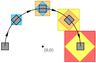
Figure 6: An illustration taken from [34] of the wrapping effect problem for a classical, idealized mathematical pendulum ODE $\ddot{x}=-x$. The picture shows a set of solutions in the phase space $(x,x^{\prime})$. The grey boxes shows the set of initial conditions (a box) moved by the flow. The coloured boxes present the wrapping effect occurring at each step when we want to enclose the moving points in a product of intervals in the basic coordinate system. For example, the blue square on the left encloses the image of the first iteration. Its image is then presented with blue rhombus which is enclosed again by an orange square. Then the process goes on. We see that the impact of the wrapping effect rapidly becomes overwhelming.

In a case of a general map $G$ one can use the mean value form for $\Phi$ to get the following:

$$\Phi(z)\in\Phi(x)+\left[D\Phi([X])\right]\cdot(X-x)$$ (52)

for all $z\in X\subset\mathbb{R}^{M}$, and the point $x\in X$ is just any point, but usually chosen to be the centre of the set $X$. Here $[X]\in\mathbb{I}^{M}$ is an interval hull of $X$ and $\left[D\Phi([X])\right]$ is an interval matrix that contains the true Jacobians $D\Phi(z)$ at all $z\in[X]$. Then, the strategy to reorganize operations depends on the shape of the set. In the simplest case let assume

$$X=x+C\cdot r_{0}+r$$ (53)

where $C$ is a linear transform $\mathbb{R}^{M}\to\mathbb{R}^{M}$, $x\in\mathbb{R}^{M}$, and with interval vectors $r_{0},r\in\mathbb{I}^{M}$ centred at $0$. Using (52) we have:

$$\Phi(z) \in\Phi(x)+\left[D\Phi([X])\right]\cdot\left(C\cdot r_{0}+r\right),$$

$$=\Phi(x)+\left(\left[D\Phi([X])\right]\cdot C\right)\cdot r_{0}+\left[D\Phi([X])\right]\cdot r$$ (54)

It is now evident, that the result set has structure similar to (53):

$$G(z)\in Y:=\bar{x}+\bar{C}\cdot r_{0}+\bar{r}.$$ (55)

With some additional reorganizations to keep $x$ and $C$ as thin as possible (e.g. point vector and matrix) and vectors $r$ and $r_{0}$ centred at $0$, we arrive at the following Lohner-type algorithm:

$$\bar{x} :=\mathtt{m}(\Phi(x)+\mathtt{Rem}(X))$$ (56)

$$S :=\left[D\Phi([X])\right]\cdot C$$ (57)

$$\bar{C} :=\mathtt{m}(S)$$ (58)

$$\bar{r} :=(S-\mathtt{m}(S))\cdot r_{0}+\left[D\Phi([X])\right]\cdot r+\left(\Phi(x)+\mathtt{Rem}(X)-\mathtt{m}\left(\Phi(x)+\mathtt{Rem}(X)\right)\right),$$ (59)

where $\mathtt{m}(\cdot)$ is an operation that returns the middle point of the interval vector or matrix. The terms in (59) might require some comments: the first term is the error left from the part $S\cdot r_{0}$ introduced by taking midpoint of matrix $S$ as $\bar{C}$ in (58). Second term is just applying mean value form on the $r$ part. Third term is the error introduced after taking midpoint of the sum in (56) as the new reference $\bar{x}$. If the matrix $\left[D\Phi([X])\right]$ and the term $\mathtt{Rem}(X)$ are ,,thin” (i.e. their entries as intervals have small diameter) then we hope the newly introduced errors should be small in comparison to the term $\bar{C}\cdot r_{0}$.

This is just one of the proposed shapes of the set in Lohner’s algorithm, the so called ,,parallelepiped ($C\cdot r_{0}$ part) with interval form of the remainder (the $r$ part is an interval box in $\mathbb{I}^{M}$)”. A more general approach is the ,,doubleton set”:

$$X=x+C\cdot r_{0}+B\cdot r$$ (60)

where matrix $B$ is chosen in some way (to be described later). The Lohner algorithm is more involved in this case:

$$\bar{x} := \mathtt{m}(\Phi(x)+\mathtt{Rem}(X))$$

$$S := \left[D\Phi([X])\right]\cdot C$$

$$\bar{C} := \mathtt{m}(S)$$

$$Q\cdot R := \mathtt{m}\left(\left[D\Phi([X])\right]\cdot B\right)$$ (61)

$$\bar{B} := Q$$ (62)

$$\bar{r} := \left(Q^{-1}\cdot\left[D\Phi([X])\right]\cdot B\right)\cdot r\ +$$

$$+ \left(Q^{-1}\cdot(S-\mathtt{m}(S))\right)\cdot r_{0}\ +$$

$$+ \left(Q^{-1}\cdot\left(\Phi(x)+\mathtt{Rem}(X)-\mathtt{m}\left(\Phi(x)+\mathtt{Rem}(X)\right)\right)\right).$$

The difference from the previous algorithm in (59) is in Eqs. (61)-(A.1). The idea of the improvement over the previous version is that one hope the first term in (A.1) to have some wrapping effect controlled by the matrix $Q^{-1}$, when doing interval enclosure. The choice about $Q$ and $Q^{-1}$ is done in Eq. (61) and depends on the algorithm implementation. Ideally, we should set $R=Id$, so that

$$Q=\mathtt{m}\left(\left[D\Phi([X])\right]\cdot B\right),$$ (64)

just as in case of (58). However, we need to compute rigorous inverse of this matrix, which might be either computationally expensive, very difficult or even impossible. On the other hand, we can choose $Q=Id$, which transforms the algorithm into the previous one (for sets with the interval form of the remainder, i.e. defined as (53)). Finally, the most commonly used method is to apply (rigorously) any QR decomposition in (61) so that the matrix $Q^{-1}=Q^{T}$ is easily obtainable. This strategy will be crucial later to get better results for DDEs in the case of $d>1$ (systems of equations).

One last remark, before we move on to the application of the Lohner’s idea in the context of DDEs, is that the method can be applied also to functions $G:\mathbb{R}^{M_{1}}\to\mathbb{R}^{M_{2}}$ where the dimensions of the domain and the image is different: $M_{1}\neq M_{2}$. Formulas (56)-(59) are all valid, but one must be very careful about dimensions of all vectors and matrices involved in the computations.

A.2 Lohner’s algorithm - complexity and optimization idea

Lohner’s algorithm complexity is dominated by the two main factors: computation of $\left[D\Phi([X])\right]$ used in (57) and multiplication of matrices. Additionally, there might be some set-structure dependent complexity, such as the need to compute the QR decomposition and the inverse of the matrix $Q$ in (61). All other operations such as matrix-vector multiplication and matrix-matrix and vector-vector additions have lower computational complexity. Computation of $\left[D\Phi([X])\right]$ cannot be avoided and has complexity depending on the complexity of the formula for $\Phi$. The complexity of matrix-matrix multiplication is $O(M^{3})$, not taking into account the possible faster (and more complicated) multiplication algorithms (e.g. Strassen’s algorithm and similar). In the rest of the appendix we will discuss the possible simple and effective optimization of those dominant operations based on the sparse structure of $\left[D\Phi([X])\right]$. We will recall from [34] that the $\left[D\Phi([X])\right]$ is very sparse in the case of the integration algorithm $\mathcal{I}$ for DDEs. We will extend and provide nicer description for the ,,fast matrix multiplication” method presented in [34] that is easily generalized for any used variables $u$ in the case of multiple delays. Moreover, later on, we will discuss possible shape of the matrix $B$ in (60) which will provide better results but without significant cost in the computational complexity.

The matrix multiplication optimization idea was first proposed in [34] for a specific case of DDEs with one delay i.e. of the form (2). Now we propose a more elegant and more general implementation, that will be suitable for implementation of the problem (26) and with $d>1$ (systems of equations). The idea is based on the decomposition of the computation of $A\cdot B$, $A\in\mathcal{M}(M,M)$, $B\in\mathcal{M}(M,N)$ into consecutive computation of products of $A_{i,\cdot}$ - $i$-th row of $A$ and $B$. In our case we think of $A$ as $A=\left[D\Phi([X])\right]$. Let assume that $A_{i,\cdot}$ has a lot of zeros (it is sparse). Let denote by $u(\cdot)$ (name conflict intentional) the following projection

$$u=(\pi_{l_{1}},\pi_{l_{2}},\ldots,\pi_{l_{k}}),\quad\forall l_{k}:A_{i,l_{k}}\neq 0$$

The function $u:\mathbb{R}^{M}\to\mathbb{R}^{k}$ and reduces the dimension of the vectors from $M$ to $k$, so we will call it a reduction. For matrix $B$ we define:

$$u(B)=\left(\begin{array}[]{c}B_{l_{1},\cdot}\\ B_{l_{2},\cdot}\\ \vdots\\ B_{l_{k},\cdot}\end{array}\right),$$ (65)

that is, $u(B)\in\mathcal{M}(k,N)$ contains all rows corresponding to the variables used in the reduction $u$. It is now easy to see that

$$A_{i,\cdot}\cdot B=u(A_{i,\cdot})\cdot u(B),$$ (66)

and the complexity of the operation is reduced from $O(M\cdot N)$ to $O(k\cdot M)$. We can now apply the multiplication in a loop for all $i$ separately, changing the $u$ accordingly (or using the same $u$ for some coordinates and do multiple rows of $A$ at the same time).

We note that, in the simplest case, when $u=(\pi_{l})$ (only one non-zero element in the $i$-th row of $A$), and $A_{i,l}=1$ we have:

$$A_{i,\cdot}\cdot B=1\cdot B_{l,\cdot}$$ (67)

and we can skip multiplication completely, changing it to a shift (selection of a given row). This will be used when $A$ has a large $Id$ block in its structure.

A.3 Lohner-type algorithm for DDEs integrator - preparation

Now we apply the Lohner strategy to our rigorous DDE integrator $\mathcal{I}$. We decompose the general method for many delays from Section 3.3 into the numerical procedure $\Phi:\mathbb{R}^{n}_{p,q}\to\mathbb{R}^{n}_{p,q+1}$ and the remainder $\mathtt{Rem}:\mathbb{R}^{n}_{p,q}\times\mathbb{I}^{d\cdot p}\to\mathbb{I}^{n}_{p,q+1}\times\mathbb{I}^{d\cdot p}$ in the following way:

$$n :=n(\eta,f)$$ (68)

$$y(u(x)) :=\left(z(x),w_{n+1}*F^{[n]}\left(u(x)\right)\right)$$ (69)

$$\Phi(a(x)) :=\left(\mathtt{T}(y(u(x));h),y(u(x)),j_{2}(x),\dots,j_{p-1}(x)\right)$$ (70)

$$\mathtt{Rem}_{A}(x,[\xi]) :=\left([F]_{[n+2]}\cdot[0,h]\cdot h^{n+1},0,\dots,0\right)\in\mathbb{I}^{n}_{p,q+1}$$ (71)

$$\mathtt{Rem}_{R}(x,[\xi]) :=\left(\frac{[0,h]}{n+2}\cdot[F]_{[n+2]},[\xi]_{2}(x),\dots,[\xi]_{p-1}(x)\right)\in\mathbb{I}^{d\cdot p}$$ (72)

where $F^{[n]}$ as in (27), $[F]$ as in (30), and $a(x)=(z(x),j(x))$ is the finite dimensional part of the description $(z,j,\xi)$ of $x$. The order $n$ of the new jet (68) comes from (28) in the algorithm, see details there. The intermediate variable $y$ is defined in (69) to shorten (70) and underline the dependence on the ,,used variables” $u(x)$. We remind that the ,,used variables” vector $u(x)$ is defined for DDE (26) with $m$ delays $\tau_{1}=p_{1}\cdot h=\tau$ (i.e. $p_{1}=p$), $\tau>\tau_{i}=p_{i}\cdot h>\tau_{j}=p_{j}\cdot h$ for $i,j\in\{2,..,m\}$, $i<j$, $p_{i},p_{j}\in\{1,..,p-1\}$ as:

$$u(x)=(z(x),j_{p_{1}}(x),j_{p_{2}}(x),\ldots,j_{p_{m}}(x)).$$

Please note that, with some abuse of notation, we can think of $u$ as a vector in $\mathbb{R}^{dim(u)}$. If $x\in C^{n}_{p}$ then $dim(u)=d(1+m\cdot(n+1))$.

First we observe that the map $\Phi$ is well defined map from $\mathbb{R}^{M}\to\mathbb{R}^{M+d}$ with $M=M(d,p,\eta)$ and it can be differentiated w.r.t. $a$ if $f$ is smooth enough, for example as in our simplifying assumption $f\in C^{\infty}$. Therefore, the Lohner algorithm might be applied ,,as it is” to the algorithm in the pair of Eqs (70)-(71) (the $A$-part of the set). However, this approach would be highly ineffective in applications, we will demonstrate now why.

A.4 Naive, straightforward implementation and the structure of $D\Phi$

For simplicity, let assume we deal with the interval representation of the error term $B\cdot r=Id\cdot r$ in the Lohner set (60) for $X=X(A,R)\subset C^{n}_{p}$. In that case, it is easy to observe that the dominant operation in the Lohner’s algorithm (in terms of computational complexity) is the matrix-matrix multiplication in Eq. (57). The application of the standard naive matrix multiplication leads to the computational complexity of $O(M^{3})=O((d\cdot n\cdot p)^{3})$ since the matrix dimensions of both $D\Phi(x)$ and $C$ dimensions are of the order of $O(d\cdot n\cdot p)$. This is also true (under some assumption) if the size of the representation $M$ grows as the algorithm is iterated. Indeed, let consider $X_{0}=X(x+C\cdot r_{0}+r,R)$ with $C\in\mathcal{M}(M,N)$ $r_{0}\in\mathbb{I}^{N}$, $r\in\mathbb{I}^{M}=\mathbb{I}^{n}_{p,0}$. Usually $N=M$, but set-up with $N\leq M$ might be beneficial in some applications. Let now consider the chain of sets $X_{i}=\Phi(X_{i-1})$ represented as Lohner’s sets (60). We have, that in the $i$-th step ($i\geq 1$) the sizes of the matrices involved in Eq. (57) are $D\Phi(X_{i})\in\mathcal{M}\left(M+d\cdot i,M+d\cdot(i-1)\right)$, $C\in\mathcal{M}\left(M+d\cdot(i-1),N\right)$ and the result matrix $S\in\mathcal{M}(M+d\cdot i,N)$. So the naive multiplication complexity is proportional to

$$(M+d\cdot i)\cdot(M+d\cdot(i-1))\cdot N\in O(M^{3}),$$

provided that both $N,i\in O(M)$ - this is usually the case, as $N>M$ does not make sense and $i>>M$ is not feasible computationally.

Please note that, for $M$ used in applications, we usually have $M\approx 1000$. Therefore the matrix-matrix multiplication in the naive implementation of Lohner’s algorithm does enormous $O(10^{9})$ operations per integration step. On the other hand, investigating Eqs. (70)-(72) reveals that the dynamics on a lot of coefficients is simply a shift to the past. Therefore, $\left[D\Phi([X])\right]$ has a following nice block structure:

$$D\Phi(v)=\left(\begin{array}[]{cccc}J_{11}(v)&J_{12}(v)&J_{13}(v)\\ J_{21}(v)&J_{22}(v)&J_{23}(v)\\ 0&Id&0\end{array}\right).$$ (73)

The matrix $J_{11}(v)\in\mathcal{M}(d,d)$ corresponds to the derivative $D_{z}\Phi_{z}(v)$, i.e. the derivative of the $z$-th component (value of the solution $x$ at current time $t=h$) w.r.t. to the change in $z(x)$ - the value of $x$ in the previous step (at $t=0$). Likewise, $J_{13}(v)\in\mathcal{M}(d,d\cdot(n+1))$ corresponds to the $D_{j_{p}}\Phi_{z}(v)$, $J_{21}(v)=D_{z}\Phi_{j_{1}}(v)\in\mathcal{M}((n+2)\cdot p,d)$, and so on. We will denote the matrix $(J_{11},J_{12},J_{13})$ as $D_{u}\Phi_{z}(v)$ and $(J_{21},J_{22},J_{23})$ as $D_{u}\Phi_{j_{1}}(v)$, respectively. Here, we use the convention that subindex such as $j_{i}$, $z$, etc. denotes the corresponding set of variables from the description of the function $x=(z,j,\xi)$.

Investigating the matrices $J_{12}(v)$ and $J_{22}(v)$ we see they correspond to the derivatives of $\Phi$ w.r.t. values at all intermediate delays $\tau_{p_{i}}$, $i>1$, so they might also contain a large number of zeros (if the equation does not depend on a particular $\tau_{i}$). When we are dealing with only one delay ($m=1$), then $J_{12}(v)=0$ and $J_{22}(v)=0$. In that case, we can apply idea proposed in the previous section A.2 to get enormous reduction in the computational complexity. We will additionally introduce the structure to the matrix $B$ defined in (60) to help with wrapping effect in the error part $B\cdot r$.

Remark 32

All matrices $J_{ij}$ in the actual implementation of the method are computed using Automatic Differentiation techniques. Those techniques can be readily applied to any equation of the form (26) as long as $f$ is a composition of simple (well known) functions like $\sin$, $\exp$, etc. and standard algebraic operations $\times$, $\div$, $+$, $-$. We do not discus details of this matter in the article.

A.5 Lohner algorithm using $D_{u}\Phi_{z}$ and $D_{u}\Phi_{j_{1}}$ directly

Let $X(A,R)\subset C^{n}_{p,q}$ be an fset such that

$$A=x+C\cdot r_{0}+B\cdot r$$ (74)

as in the Lohner structure (60) where $C\in\mathcal{M}(M,N)$, $M=\mathtt{dim}(\mathbb{R}^{n}_{p,q})$. The matrix $B$ will have a special block-diagonal:

$$B=\left(\begin{array}[]{ccccc}B_{z}&0&\cdots&0\\ 0&B_{j_{1,[0]}}&0&\ddots\\ \vdots&0&\ddots&\ddots\\ 0&\vdots&\ddots&B_{j_{p,[\eta_{p}]}}\end{array}\right),$$ (75)

where each $B_{b,b}\in\mathcal{M}(d,d)$.

Now, we can apply (55) to the pair of methods $(\Phi,\mathtt{Rem}_{A})$ in Eqs. (70)-(71) to get a new fset of the same structure $Y=X(\bar{x}+\bar{C}\cdot r_{0}+\bar{r},\mathtt{Rem}_{R}(X))\subset C^{n}_{p,q+1}$ so that for all $z\in X(A,R)$ we have $\varphi(h,z)\in Y$. Please note, that $\bar{C}\in\mathcal{M}(M+d,N)$, $\bar{r}\in\mathbb{R}^{n}_{p,q+1}=\mathbb{R}^{M+d}$ and $r_{0}\in\mathbb{R}^{N}$ stays the same as in the original Lohner’s algorithm (this is important). The extra $d$ rows in matrix $\bar{C}$ are due to the extra Taylor coefficient computed at $t=0$. In general, in $i$-th iteration of the algorithm the matrix $C_{i}$ will be of the dimension $\mathcal{M}(M_{0}+d\cdot i,N)$ and the error term $r$ will be of dimension $\mathbb{R}^{M_{0}+d\cdot i}$, $B\in\mathcal{M}(M_{0}+d\cdot i,M_{0}+d\cdot i)$, where $M_{0}=M(d,p_{0},\eta_{0})$ is the dimensional of the initial set $X_{0}\in C^{\eta_{0}}_{p_{0}}$ at the beginning of the integration process. In applications, we usually set $N=M_{0}$.

Remark 33

There is a slight abuse of notation here, as we are using $x$ to denote the base point of the set $A$ and, at the same time, usually it denotes the segment of the solution $x\in X$. However, the two are used in a different context, so it should not create confusion (one is the Lohner’s set of the $A$ part in $X(A,R)$, second is as an element of $X(A,R)$). We will state explicitly if $x\in X$ otherwise $x$ always denotes the mid point of $A$. Please also note, that, by definition, if $x\in X$, then naturally $a(x)\in A=x+C\cdot r_{0}+B\cdot r$.

Now, the crucial part is to look at each $d$-dimensional variable $z(X)$ and $j_{i,[k]}(X)$ as a separate Lohner’s set with its own structure inherited from the full set $X=X(A,R)$ and apply the Lohner’s algorithm separately on each part, together with the optimization idea from A.2.

A.5.1 The convention

As with the $u$ in (65), for a matrix $C\in\mathcal{M}(M,N)$ we define $z(C)$ and $j_{i,[k]}(C)$ as the matrix containing all the appropriate rows from $C$. Each $z(C)$ and $j_{i,[k]}(C)$ is therefore a matrix in $\mathcal{M}(d,N)$.

It is easy to see that if the set $X=X(A,R)$, with $A$ as in (74), then

$$z(X)=z(x)+z(C)\cdot r_{0}+B_{z}\cdot z(r),$$

where $B_{z}\in\mathcal{M}(d,d)$ given as in (75) and $z(C)\in\mathcal{M}(d,M)$. Similarly $j_{i,[k]}(X)=j_{i,[k]}(x)+j_{i,[k]}(C)\cdot r_{0}+B_{j_{i,[k]}}\cdot j_{i,[k]}(r)$.

Remark 34

The use of the abstract operations $z(\cdot)$, $j_{i,[k]}(\cdot)$, and $u$ allows for a more general implementation of the methods, independent of the actual storage organization of the data in computer programs.

A.5.2 The shift part

First consider easy case of computing $j_{i}(\bar{X})$ in $\bar{A}=\Phi(a(X))$ for $i>1$. We observe that

$$D_{j_{l}}\Phi_{j_{i}}(a(X))=\begin{cases}Id_{d\times d}&l=i-1\\ 0_{d\times d}&otherwise\end{cases}.$$

as this is the case of the shift to the past in Eq. (21). The procedure is exact (i.e. $\mathtt{Rem}_{A}(X)_{j_{i}}=0$, see Eq. (71)) and no extra errors are introduced. Therefore:

$$j_{i}(\bar{X})=j_{i-1}(X),$$

and using observation (67) we have for all appropriate $k$:

$$j_{i,[k]}(\bar{C}) = j_{i-1,[k]}(C)$$

$$j_{i,[k]}(\bar{x}) = j_{i-1,[k]}(x)$$

$$\bar{B}_{j_{i,[k]}} = B_{j_{i-1,[k]}}$$ (76)

$$j_{i,[k]}(\bar{r}) = j_{i-1,[k]}(r).$$ (77)

With a proper computer implementation those assignment operations could be avoided completely, for example by implementing some form of pointers swap or just by designing the data structures to be easily extended to accommodate new data. This last approach is implemented in our current source code so that the computational complexity is negligible.

What is left to be computed are two parts: $j_{1}(\bar{X})$ and $z(\bar{X})$.

A.5.3 The $\Phi_{j_{1}}$ part

From (70) we have

$$\Phi_{j_{1,[k]}}(a(x))=\left(y\left(u(x)\right)\right)_{[k]}=\left(z(x),w_{n+1}*F^{[n]}\left(u(x)\right)\right)_{[k]}.$$

It is obvious that $\Phi_{j_{1,[k]}}$ as a function of the variables $a$ is in fact a function only of the subset of variables $u$, so is the function

$$\Phi_{j_{1}}=\left(\Phi_{j_{1,[0]}},\Phi_{j_{1,[1]}},\ldots,\Phi_{j_{1,[n(f,\eta)]}}\right)$$

Therefore, with some abuse of notation, we can define $D_{u}\Phi_{j_{1}}(u)$ for all $u\in u(X)$. This is a matrix $\mathcal{M}(K,dim(u))$ with $K=(1+n(f,\eta))\cdot d$ and is given by:

$$D_{u}\Phi_{j_{1}}=\left(\begin{array}[]{c}D_{u}\Phi_{j_{1,[0]}}\\ D_{u}\Phi_{j_{1,[1]}}\\ \vdots\\ D_{u}\Phi_{j_{1,[n(f,\eta)]}}\end{array}\right).$$

This way we can skip the computation of many entries in $D\Phi_{j_{1,[k]}}$.

Applying the trick from Eq. (66) on each row of $D\Phi_{j_{1}}\cdot C$ we get:

$$D\Phi_{j_{1}}(u)\cdot C=D_{u}\Phi_{j_{1}}(u)\cdot u(C).$$ (78)

The dimension of matrices taking part in the multiplication on the right side are $\mathcal{M}(K,dim(u))$ and $\mathcal{M}(dim(u),N)$. Therefore, the cost of the computation is $O(K\cdot dim(u)\cdot N)$ instead of $O(K\cdot M\cdot N)$ when performing the multiplication on the left.

A.5.4 The $\Phi_{z}$ part

Similarly as before, we treat $\Phi_{z}(a(x))$ as a function of only used variables $\Phi_{z}(u(x))$. It has an explicit formula:

$$\Phi_{z}(u(x))=\mathtt{T}(y(u(x));h)=\sum_{k=0}^{n(f,\eta)}\Phi_{j_{1,[k]}}(u(x))\cdot h^{k},$$

so that the Jacobian $D_{u}\Phi_{z}(u)$ has a known form expressed in terms that are already computed:

$$D_{u}\Phi_{z}(u)=\sum_{k=0}^{n(f,\eta)}D_{u}\Phi_{j_{1,[k]}}(u(x))\cdot h^{k}.$$ (79)

Therefore, the computation of $D_{u}\Phi_{z}$ is computationally inexpensive in comparison to the matrix-matrix multiplication.

Applying again the trick from Eq. (66) on each row of $D\Phi_{z}\cdot C$ and the Eq. (79) we get:

$$D\Phi_{z}(u)\cdot C = \sum_{k=0}^{n(f,\eta)}\left(D_{u}\Phi_{j_{1,[k]}}(u)\cdot u(C)\right)\cdot h^{k}\ =$$

$$= \sum_{k=0}^{n(f,\eta)}\left(j_{1,[k]}\left(D_{u}\Phi_{j_{1}}(u)\cdot u(C)\right)\right)\cdot h^{k},$$

where the matrix term $D_{u}\Phi_{j_{1}}(u)\cdot u(C)$ is already computed in Eq. (78). Therefore the cost of this operation consists only of additions and scalar-matrix multiplication, thus may be neglected in comparison to other operations in the Lohner-type algorithm.

A.5.5 Summary computational cost of $D\Phi\cdot C$ multiplication

Taking all into account, we get that computing the matrix-matrix multiplication of the Lohner-type algorithm applied to the integration scheme for DDEs is dominated only by the multiplication $D_{u}\Phi_{j_{1}}(u)\cdot u(C)$ in (78). Its cost is $O(K\cdot dim(u)\cdot N)$ with $K=(1+n(f,\eta))\cdot d$ which is a big reduction from $O(M^{2}\cdot N)$. To better see this, note that $dim(u)\leq M$ and assuming $\eta_{i}=n$ for all $i$ (for simplicity) we have $M=d\cdot(1+(n+1)\cdot p)=O(d\cdot n\cdot p)$. In that case $K=d\cdot(n+2)$ and we get the upper estimate on the complexity $O(d\cdot n\cdot M\cdot N)=O(d^{2}\cdot n^{2}\cdot p\cdot N)$. The naive implementation has the complexity $O(d^{2}\cdot n^{2}\cdot p^{2}\cdot N)$. Moreover, if we assume a constant and small number of delays used in the definition of r.h.s. $f$ of equation (26), $m=const<<p$ then we get complexity of order $O(d^{2}\cdot n^{2}\cdot N)$ - a reduction of the factor $p^{2}$. Noting that $p$ is usually the biggest of the parameters $d,p,n$ (see applications), we get an enormous reduction in the computation times, making the algorithm feasible to be applied for a variety of problems. To see how big is the reduction let assume $p=128$, $n=4$, $d=1$ and $N=M$ as in the Mackey-Glass examples. We get $(dpn)^{3}=134217728$ of order $10^{8}$, whereas $d^{2}\cdot n^{2}\cdot M=10256$ of order $10^{4}$.

A.5.6 QR decomposition on $\Phi_{z}$, $\Phi_{j_{1}}$ parts in the case $d>1$

Up to now we only focused (57) in the Lohner-type algorithm for DDEs. Now, we need to return to the problem of managing local errors - the part $B\cdot r$ in (60), and the formulas in Eqs. (61)-(A.1).

First we note that the structure of matrix $B$ in (74) is block diagonal (75). We want to create a matrix $\bar{B}$ in the representation of $\Phi(X)+\mathtt{Rem}(X)$ of the same structure. The choice of the block-diagonal structure of $B$ is dictated by the need to compute $Q^{-1}=\bar{B}^{-1}$ in (A.1). We cannot hope to be able to rigorously compute decomposition $Q\cdot R$ or rigorously invert a big and full matrix $\bar{B}$, as those operations are ill-conditioned and very costly ($O(M^{3})$). The sparse diagonal matrix $B$ removes both those problems with the trade-off in a form of more complicated algorithm and some extra error terms.

We have already used the structure of $B$ in Eqs. (76)-(77) to reduce problem complexity significantly for the shift part, i.e. computing $\bar{B}_{j_{i},[k]}$ for all $i>1$. What is left to compute is $\bar{B}_{j_{1},[k]}\in\mathcal{M}(d,d)$ and $\bar{B}_{z}\in\mathcal{M}(d,d)$.

To define appropriate $Q_{j_{1,[k]}}=\bar{B}_{j_{1,[k]}}$ and a new $j_{i,[k]}\left(\bar{r}\right)$ we investigate the term $\left[D\Phi([X])\right]\cdot B\cdot r$ from Eq. (A.1). Taking projection onto the $j_{1,[k]}$-th coordinate and using the $u$-variable trick we get:

$$j_{1,[k]}\left(\left[D\Phi([X])\right]\cdot B\cdot r\right) = \left[D_{u}\Phi_{j_{1,[k]}}([X])\right]\cdot u(B)\cdot u(r)\ =$$

$$=: D\cdot u(B)\cdot u(r),$$

with $D=\left[D_{u}\Phi_{j_{1,[k]}}([X])\right]$ for a shorter notation. A close inspection reveals that $D\cdot u(B)\in\mathcal{M}(d,dim(u))$. Such a matrix is not suitable to apply the QR strategy of the Lohner’s set. We expand further:

$$D\cdot u(B)=\left(\begin{array}[]{ccccc}D_{z}\cdot B_{z}&D_{j_{p_{1},[0]}}\cdot B_{j_{p_{1},[0]}}&D_{j_{p_{1},[1]}}\cdot B_{j_{p_{1},[1]}}&\cdots&D_{j_{p_{m},[\eta_{p_{m}}]}}\cdot B_{j_{p_{m},[\eta_{p_{m}}]}}\end{array}\right),$$

where $D_{j_{q,[s]}}=\left[D_{j_{q,[s]}}\Phi_{j_{1},[k]}([X])\right]\in\mathcal{M}(d,d)$. Now, the term $D\cdot u(B)\cdot u(r)$ can be computed as follows:

$$D\cdot u(B)\cdot u(r)=\left(D_{z}\cdot B_{z}\right)\cdot r_{z}+\sum_{j_{i,[k]}\in u}\left(D_{j_{i,[k]}}\cdot B_{j_{i,[k]}}\right)\cdot r_{j_{i,[k]}}$$ (81)

Now, a decision has to be made, as to which $I\in u=(z,j_{p_{1},[0]},j_{p_{1},[1]},\ldots)$ to choose for the QR decomposition:

$$Q_{j_{1,[k]}}\cdot R_{j_{1,[k]}}=\mathtt{m}(D_{I}\cdot B_{I}).$$

and to compute $\bar{r}_{j_{1,[k]}}$ according to (A.1):

$$\bar{r}_{j_{1,[k]}} = \left(Q_{j_{1,[k]}}^{-1}\cdot D_{z}\cdot B_{z}\right)\cdot r_{z}+\sum_{j_{i,[k]}\in u}\left(Q_{j_{i,[k]}}^{-1}\cdot D_{j_{1,[k]}}\cdot B_{j_{i,[k]}}\right)\cdot r_{j_{i,[k]}}\ +$$ (82)

$$+ \left(Q_{j_{1,[k]}}^{-1}\cdot j_{1,[k]}\left(S-\mathtt{m}(S)\right)\right)\cdot r_{0}\ +$$ (83)

$$+ Q_{j_{1,[k]}}^{-1}\cdot\left(\Phi_{j_{1,[k]}}(x)+\mathtt{Rem}_{j_{1,[k]}}(x)-\mathtt{m}\left(\Phi_{j_{1,[k]}}(x)+\mathtt{Rem}_{j_{1,[k]}}(x)\right)\right)$$ (84)

The matrix-matrix and matrix-vector operations are done in the order defined by parentheses. Note, that all operations are well defined. The dimensions of the matrices are as follows: $Q_{j_{1,[k]}}^{-1},D_{J},B_{J}\in\mathcal{M}(d,d)$, and $j_{i,[k]}(S)\in\mathcal{M}(d,N)$ for all variables $J\in u$. The vectors are: $r_{0}\in\mathbb{I}^{N}$ while $r_{J},\Phi_{j_{1,[k]}}(x),\mathtt{Rem}_{j_{1,[k]}}(x)\in\mathbb{I}^{d}$.

Remark 35

The same algorithm might be used to compute $\bar{r}_{z}$. We only change the projection $j_{1,[k]}$ to $z$ in the presented formulas.

A.5.7 Complexity of handling doubleton set structure

The computational cost of using QR strategy with the doubleton set structure (60) in comparison to the interval form of the error terms in the basic structure (53) is as follows. In the basic set structure the operation (59) is exactly realized by the presented algorithm when we take $Q=Id_{d\times d}$ and we use fact that each $B_{J}=Id$. We can of course skip multiplication by $Id$. Therefore, the cost of operations is (we count scalar multiplications):

• for (82): $\frac{dim(u)}{d}\cdot d^{2}=d\cdot\dim(u)$

• for (83): $d\cdot N$,

• for (84): $0$ (no matrix-matrix and matrix-vector multiplications).

In total, we get that computing $\bar{r}_{J}$ for each $J\in\left\{z,j_{1,[0]},\ldots,j_{1,[n]}\right\}$ is $O\left(d\cdot(dim(u)+N)\right)$. Taking into account $dim(u)\leq M$ and $d<<M$, together with the assumption $N=M$ (in applications) we get the complexity $O(d\cdot M)=O(M)$ under assumption that $d=const$, small.

The algorithm for the doubleton set (60) with non-trivial QR-decomposition has the following complexity for each $\bar{r}_{J}$:

• cost of computing QR decomposition for a matrix $D_{I}\cdot B_{I}\in\mathcal{M}(d,d)$, usually it is $O(d^{3})$ multiplications,

• cost of computing $Q^{-1}$, should not exceed $O(d^{3})$, but it is usually $O(1)$ - if $Q$ is chosen to be orthogonal,

• for (82): $\frac{dim(u)}{d}\cdot\left(d^{3}+d^{3}+d^{2}\right)=O(d^{2}\cdot\dim(u))$

• for (83): $d^{2}\cdot N+N\cdot d=O(d^{2}\cdot N)$,

• for (84): $d^{2}$.

In total, the complexity is $O\left(d^{2}\cdot(d+dim(u)+N)\right)$. Under the same assumptions as before, we estimate that in applications the complexity is $O(d^{2}\cdot M)$. Therefore, handling the proposed doubleton structure is not much more costly than using the interval form of the remainder (at least for small $d$).

Remark 36

Please note, that the current strategy does not help in the scalar case $d=1$. The two sets are in this case equivalent and the computational cost is basically the same.

A.5.8 Choice of the matrix $D_{I}\cdot B_{I}$ for the QR procedure

As to the selection of the matrix $D_{I}\cdot B_{I}$ used in the QR decomposition procedure, in our current implementation we always use $I=z$. The motivation is as follows: in our applications to the Rössler system we apply the method to a perturbed system $x^{\prime}(t)=f(x(t))+\varepsilon\cdot g(x(t-\tau))$ with $\varepsilon$ small. Therefore, we expect that the influence $D_{J}\cdot B_{J}$ for $J\neq z$ will be small. Taking $I=z$ allows to compare the method to the ODE version of the proofs. Indeed, if we set $\varepsilon=0$ and integrate the problem with our code, all $D_{J}=0_{d\times d}$ and the method (82)-(84) reduces to that of the ODE (we only do operations on $z$ coordinate).

Other choices of $I$ are easily implementable and one might want to pursue other forms of the matrix $B$, for example using various size blocks $B_{j_{i}}$ that does QR decomposition on more than $d$ dimensions.

Appendix B Description of the data and computer programs

In this appendix we present details of the methodology to generate initial sets for computer assisted proofs. As the data sets are large, one cannot hope to select good initial set candidates ,,by hand”, as can be done sometimes in the context of low-dimensional ODEs or maps. Instead, some kind of automatic or semi-automatic procedure must be used.

B.1 Source codes and a virtual machine

The compressed archive of the source codes can be downloaded from the web page [30]. A file README.txt from the main directory contains information on dependencies, compiling process and running the programs on the user’s own computer. For a users not wanting to compile files by themselves, we made an image of a virtual machine (VM) with Linux system, all compiler tools, and the source codes compiled to executables that were used to produce data for this paper. It can be downloaded from [31], where one also find the instructions for running the virtual machine. A computer running Docker VM on a Linux system is needed to use the virtual machine image. We recommend following instructions on the official web page: https://docs.docker.com/engine/install/ and selecting the user’s system.

B.2 List of programs used in computer-assisted proofs

All the programs used in proofs reside in the subdirectories placed under the root directory of the compressed archive or in the directory /home/user/DDEs in the VM image. This root directory is common for all programs, and in what follows we give paths relative to this root directory. The programs can be found in the ./examples subdirectory. The data for the proofs used in this paper can be found in ./results subdirectory.

B.2.1 The program used to produce data in Table 1

The programs used for benchmark in Table 1 can be found in ./examples/benchmark. The program can be compiled by issuing the following command in the main directory of the source codes:

make benchmark

To obtain data from table 1 one needs to invoke the following command in the ./bin/examples/benchmark directory:

./benchmark diam=’[0,0]’ xi=’[0,0]’ dirpath=’table-1’

Results of the computations will be stored in ./bin/examples/benchmark/table-1 and will consist of several files (.tex, .pdf, .png, .dat, etc.). One need latex and gnuplot packages installed in the host system for the program to work correctly. One can make various tests by changing the parameters. The full list of parameters is presented below:

./benchmark \ 
initial=’{[1.1,1.1]}’ \ 
dirpath=’.’ \ 
prefix=’benchmark’ \ 
N=’[8,8]’ \ 
n=’4’ \ 
p=’128’ \ 
epsi=’50\%’ \ 
diam=’[-1e-06,1e-06]’ \ 
xi=’[-0.1,0.1]’ 

The values on the right of = are the default values. It is important to put the parameters into single quotes ’...’. The system modelled by the program is Mackey-Glass equation with $\gamma=1$, $\beta=2$, $\tau=2$ and $n=$ N (do not confuse with $n$ in the definition of $C^{n}_{p}$. Parameter initial represents $x_{0}$ in the definition of the initial Lohner set $X(A_{0},R_{0})$, $A_{0}=x_{0}+Id\cdot r_{0}$, $r_{0}$ given by diam (see later). Parameter initial can either be an interval, in that case the program will treat $x_{0}$ as a representation of a constant initial function $x_{0}\equiv$ initial; or it can be a path to a file containing a vector describing the $(z,j)$ part of the initial segment. For examples of such files, please refer to initial data in the computer assisted proofs. Parameter dirpath describes the directory of the output files from the program. It is advised to select non-existing folder, as the program overwrites existing files without asking. Parameter prefix will be appended in front of all filenames. Parameters n, p corresponds to $n$, $p$ in $C^{n}_{p}$, and are the order of the representation and the number of grid points on the base interval $[-2,0]$, respectively. The full step $h=\frac{2}{p}$. Parameter epsi corresponds to $\varepsilon$ step done to simulate computation of the Poincaré map, and can be given as a percentage of the full step $h$ or as an explicit interval. Parameter diam is the diameter $r_{0}$ of the $A_{0}=x_{0}+Id\cdot r_{0}$ part in $X(A_{0},R_{0})$, while xi is the diameter of $R_{0}$.

B.2.2 The programs used in the proof of Theorem 28

The programs used in the proof of Theorem 28 reside in the following subdirectories:

• ./examples/rossler_delay_zero for the Rössler original ODE (46), but studied in the extended space $C^{n}_{p}$ over the base delay interval $[-1,0]$. Programs in this directory are used to generate common set for all the proofs.

• ./examples/rossler_delay_rossler for the delayed perturbation of the form $g=f$.

• ./examples/rossler_delay_other for the delayed perturbation $g$ given in (49).

Each of the directories contain the following programs

• nonrig_attractor (non-rigorous, approximate), it is used to generate initial set of functions to be used in the program nonrig_coords. It generates also plot to view the structure of the apparent attractor.

• nonrig_coords (non-rigorous, approximate) it computes first approximation of the coordinate frame for the set $A$ in the definition of the set $X(A,R)$. The program uses the output of the program nonrig_attractor to generate a set $S$ of several hundred solution segments lying on the section $S_{0}$. Due to the nature of Rössler attractor, those segments are contained in a thin strip over $(x,y)$-plane (set is thin in $z$ direction), see Fig. 3. Then, a reference solution $v_{ref}$ segment is selected as the one closest to the centre of this collection. Let denote by $|S|$ the number of solution segments in $S$. We define:

  $$w^{i} = v^{i}-v_{ref},\quad v^{i}\in S\setminus\{v_{ref}\},$$

  $$u^{i} = \frac{u^{i}}{u^{i}_{2}},$$

  $$u = \frac{\sum u^{i}}{|S|-1}$$

  or, in other words, $u$ is the mean vector that spans the intersection of the apparent Rössler attractor with the section $S_{0}$. The vector is normed in such a way that $u_{2}=1$. This corresponds to $\pi_{y}u=1$. The initial coordinate frame is chosen to be:

  $$\tilde{C}=\left(\begin{array}[]{ccccc}1&&0&\cdots&0\\ 0&&0&\cdots&0\\ \vdots&u^{T}&&&\\ \vdots&&&Id_{(M-2)\times(M-2)}&\\ 0&&&&\end{array}\right),$$ (85)

  that is, first column corresponds to the normal vector to the section hyperplane $S_{0}=\{v:\pi_{x}v(0)=0\}$, the second column corresponds to the nominally unstable direction $u$, and the rest of coordinates are just the canonical basis in $\mathbb{R}^{M-2}$. The set $X(A,\Xi)$ is then defined with: $A=v_{ref}+\tilde{C}\cdot r_{0}$, with $r_{0}$ to be defined by the next program rig_find_trapping_region.

• rig_find_trapping_region (rigorous) as input, it takes the width $W=[W_{l},W_{r}]$ of the set in the nominally unstable direction $u$ and the coordinate frame $v_{ref}$ and $\tilde{C}$. Then it starts with $A^{0}=v_{ref}+\tilde{C}\cdot r$ with $r_{1}=0$, $r_{2}=W$, $r_{i}=(-\epsilon,\epsilon)$ for some small $\epsilon$ for $i>2$. Then it tries to obtain the set $X(A,\Xi)$ iteratively ,,from below”, i.e. at each step $k=0,1,...$ it computes image $P(X(A^{k},\Xi))$ and checks if it is subset of $X(A^{k},\Xi)$. If the test is passed, the program stops, otherwise it takes $A^{k+1}=\mathtt{hull}(A^{k},\pi_{A}P(X(A^{k},\Xi)))$ and continues to the next step. The computation of $P(X(A^{k},\Xi))$ is done by dividing the input set into $N$ pieces along the nominally unstable direction $r_{2}$. For proofs used in this work $N=200$.

  Finally, when the set $A$ is found, the coordinate frame $\tilde{C}$ is changed (by rescaling) to $C=\tilde{C}\cdot\mathrm{Diag}(r)$ so that $A=v_{ref}+C\cdot\left(\{0\}\times W\times\operatorname{\mathbf{B}}^{\|\cdot\|_{\infty}}_{M-2}(0,1)\right)$. The matrix $\mathrm{Diag}(r)$ denotes the diagonal matrix with $r_{i}$’s on the diagonal.

• rig_prove_trapping_region_exists (rigorous) the program computes the image of the set $X(A,\Xi)$ under the Poincaré map $P:S_{0}\to S_{0}$. If the rig_find_trapping_region is successful in finding the rigorous candidate $A$, then this program must succeed, as it computes the image $P(X(A,\Xi))$ in the same way, dividing the set into the same $N$ pieces.

• rig_prove_covering_relations (rigorous) the program checks the conditions (CC2A) and (CC2B) of Lemma 26 on sets $X(N_{1},\Xi)$ and $X(N_{2},\Xi)$. The sets are defined as the restrictions of the set $X(A,\Xi)$ on the nominally unstable direction $r_{2}$. The user can manipulate the definitions of sets changing the values in the configuration file rig_common.h.

Remark 37

To prepare the set $X(A,\Xi)$ for the Theorem 28, we run rig_find_trapping_region for the system without the delay first. Then we use it again on the resulting set for the delayed systems. In this way we obtain three sets $A_{0}$ for the unperturbed system, $A_{f}$ for $g=f$ and $A_{g}$ for the system with $g$ given as in (49). As the final set $A$ we take $A=\mathtt{hull}(A_{0},A_{f},A_{g})$. The computer assisted proofs show that this set is a trapping region for all systems.

The data used in the proofs can be found for each of the systems in the respective directories:

• ./results/work3_rossler_delay_zero,

• ./results/work3_rossler_delay_rossler,

• ./results/work3_rossler_delay_other.

B.2.3 The programs used in the proof periodic orbits in the Mackey-Glass equation

The programs used in the proof of Theorem 31 can be found in ./examples/mackey_glass_unstable. There is a single program for each of the orbits: prove_T1, prove_T2, and prove_T4, respectively. The data for the proofs is stored in ./results/work3_mackey_glass_proofs. Additionally, a set of generic programs to generate the flow, coordinates and sets for proofs are available in ./examples/mackey_glass_finder. The programs comprise a full set of tools that once compiled can be used to find candidates for periodic solutions to Mackey-Glass equation for any set of parameters and later to prove their existence. With a little effort the programs can be adjusted to work with any scalar DDE - small changes in the file constans.h should suffice. The collection of programs is as follows:

• attractor-coords-nonrig non-rigorous program to generate good coordinates for presentation of the Mackey-Gass attractor (used for parameters in chaotic regime).

• compare-rig a program to compare two interval sets and print the comparison in a human-friendly manner.

• draw-nonrig non-rigorous program to draw solutions in various ways.

• find-nonrig a non-rigorous Newton-like method to refine the non-rigorous candidate for a periodic solution with high accuracy.

• jac-poincare-nonrig a program to compute non-rigorous image of the Poincaré map $P$ for a single initial condition $x$, together with the (approximate) Jacobian $DP(x)$.

• periodic-coords-nonrig a program to generate the ,,good” basis for the set $X(A,R)$. The procedure is described in more details later in this Appendix.

• poincare-nonrig a program to compute non-rigorous Poincaré map for a collection of initial conditions.

• poincare-rig a program to compute rigorously the image of the Poincaré map $P$ on a (p,n)-fset $X(A,R)\subset C^{n}_{p}$.

• simple-coords-nonrig alternative program to generate very simple coordinates, where majority of base vectors comes from the cannonical basis.

An exemplary process of finding good candidates and initial sets for orbits $T1$, $T2$ and $T4$ can be found in the subdirectory ./results/work3_mackey_glass_finder. The scripts contained there was used to generate data for this paper and they are as follows ($i $\in\{1,2,4\}$):

• setup.sh a common setup script for all other scripts. In principle, user only edit this file.

• T$i-1-make-coords.sh uses some aforementioned programs to refine the candidate solution $x_{0}$ (mid point of the set) and generate good coordinates for the fset $X(A,\Xi)$, with $A=x_{0}+C\cdot r_{0}$.

  In case of the solution $T4$, the script is more complicated as it finds a pair of sets $X_{1}=X(A_{1},\Xi_{1})$, $X_{2}=X(A_{2},\Xi_{2})$ for the covering $X_{1}\stackrel{{\scriptstyle P_{1}}}{{\Longrightarrow}}X_{2}\stackrel{{\scriptstyle P_{2}}}{{\Longrightarrow}}X_{1}$, where $P_{1},P_{2}$ are two Poncaré maps, defined between two different sections.

• T$i-2-find-start.sh try to do the first step of an algorithm to find appropriate $r_{0}$ and $\Xi$ such that $X(A,\Xi)\stackrel{{\scriptstyle P}}{{\Longrightarrow}}X(A,\Xi)$. It starts with a thin set $x_{0}+C\cdot\{0\}\times W\times[0,0]^{M}-2$ and build the set $X_{1}=P(X)$. The sets are set to have the first coordinate of width $W$ (guessed by the user, similarly to the building sets in the Rössler case).

  The procedure is more involved in the case of $T4$, as there are two sets $X_{1}$ and $X_{2}$ on different sections such that we hope $X_{1}\stackrel{{\scriptstyle P_{1}}}{{\Longrightarrow}}X_{2}\stackrel{{\scriptstyle P_{2}}}{{\Longrightarrow}}X_{1}$. The program tries to find both sets at the same time.

• T$i-3-find-once.sh subsequent iteration of the previous algorithm. The user needs to run this script until satisfactory $r_{0}$ and $\Xi$ is found. This part of the finding procedure is semi-automatic, as the decision when to stop the procedure is left to the user.

  The data generated by the authors of this manuscript can be found in the following directory: ./data/examples/mg.

• T$i-4-proof.sh the script runs the final check of the covering relations in the proof of Theorem 31. If the $W$ width in the unstable direction was set improperly in the previous steps (too narrow), then the script might fail to prove the covering relation.

  In case of $T1$ and $T2$ the program checks the simplest covering relation $X\stackrel{{\scriptstyle P}}{{\Longrightarrow}}X$. In case of $T4$ the covering relation to check is more involved: $X_{1}\stackrel{{\scriptstyle P_{1}}}{{\Longrightarrow}}X_{2}\stackrel{{\scriptstyle P_{2}}}{{\Longrightarrow}}X_{1}$, where $P_{1},P_{2}$.

B.2.4 Idea of the coordinate selection

The following procedure is adopted in the program periodic-coords-nonrig for choosing right coordinates for periodic orbits proofs. Each set $V_{i}=X(A_{i},\Xi_{i})$ with $A_{i}=\bar{T}^{i}_{0}+C_{i}\cdot r_{i}$. The matrix $C_{i}$ must be computed carefully, as it was shown in [34] and in more details in [12]. In short, one expects that the linearized dynamics near the stationary point $\bar{T}^{i}_{0}$ of the Poincaré map $P^{i}$, $i\in 1,2,4$ should decompose into invariant subspaces $E_{c}\oplus E_{u}\oplus E_{s}$ with $dim(E_{c})=dim(E_{u})=1$. The subspace $E_{c}$ corresponds to the direction along the flow, where $E_{u}$ is the unstable space of solutions that have a backward in-time limit at the fixed point, where $E_{s}$ is the space of those solutions that approach the fixed point as $t\to+\infty$. The matrix $C_{i}$ is chosen as a composition of the bases of appropriate subspaces:

$$C_{i}=\left(\begin{array}[]{ccccc}c^{T}&u^{T}&s_{3}^{T}&\ldots&s_{M}^{T}\end{array}\right),$$ (86)

where we have:

• $c$ is the vector defining a section and is chosen in the program as a left eigenvector (i.e. eigenvector of the transposed matrix) of the approximate matrix $\overline{DP}(\bar{T}^{i}_{0})$ corresponding to the eigenvalue $\lambda_{2}=1$.

• $u$ is the eigenvector of $\overline{DP}(\bar{T}^{i}_{0})$ corresponding to the largest and unstable eigenvalue $\lambda_{1}$ with $|\lambda_{1}|>1$.

• the set of vectors $s_{j}$ is the basis of the (finite projection) of the stable subspace $E_{s}$. It is obtained as an orthonormal basis orthogonal to the vector $\tilde{u}$ - the left eigenvector corresponding to the unstable eigenvalue $\lambda_{1}$.

The reason why those are chosen as described is explained in details in [34, 12] and we skip the details here. We only hint that the selection of $c$ guarantees to have a very thin interval $[t_{p}(X)]$ in rigorous computations of Poincaré maps, where selection of $s_{3},\ldots s_{M}$ gives a hope that the finite dimensional projection of the $P(X)$ onto stable subspace $E_{s}$ could be mapped inside the stable part of the initial set $X$ ($\pi_{E_{s}}P(X)\subset\pi_{E_{s}}X$) without the need to resort to a set subdivision in computations.

B.2.5 Utility programs

The programs in directory ./examples/converter are used in some other scripts to do conversion between different kinds of data, for example making interval versions of vector/matrices from their double counterparts. One important program is the matrix converter convmatrix that can compute rigorously in high precision the rigorous inverse of interval matrix. For more information how to use those programs, see their source code documentation. The list of utility programs is as follows:

• convmatrix a conversion between various formats of matrices. It can compute rigorous inverse of a matrix in high precision.

• convvector a conversion between various formats of vectors.

• growvector converts an interval vector $[x]$ into $[w]=\mathtt{m}([x])+r\cdot\left([x]-\mathtt{m}([x])\right)$, for some $r\in\mathbb{R}$.

• splitvector converts an interval vector $[x]$ into $[w]=\mathtt{m}([x])$ and $[v]=[x]-\mathtt{m}([x])$.

• crmatrix takes a matrix $C$ and a vector $r$ and makes a rigorous matrix $C_{r}$ such that $C\cdot r\subset C_{r}\cdot[-1,1]^{M}$.

• rmatrix takes a vector $r$ and makes a rigorous matrices $R$ and $R^{-1}$ such that $R_{i,i}=r_{i}$, $R_{i,j}=0$ otherwise.

• invmatrixtest performs a test if the pair of matrices $A$ and $B$ given on input has the property that $Id\subset A\cdot B$ and $Id\subset B\cdot A$. Computes also the width (maximal diameter of all entries) of $A\cdot B$ and $B\cdot A$, allowing to assess the quality of computed inverses.

• matrixcmp compares two (large) matrices in a human-friendly manner.

• midmatrix compute $\mathtt{m}(A)$ for a matrix $A$.

• vectorcmp compares two (large) vectors in a human-friendly manner.

• vectorhull compute an interval hull of all vectors given on input.

References

- [1] F.A. Bartha, T. Krisztin, and A. Vigh. Stable periodic orbits for the Mackey-Glass equation. J. Differential Equations, 296:15–49, 2021.
- [2] RF. Brown. A Topological Introduction to Nonlinear Analysis. Second Edition. Springer Science+Business Media New York, 2004.
- [3] K.E.M. Church. Validated integration of differential equations with state-dependent delay. Commun. Nonlinear Sci. Numer. Simul., 115:DOI:10.1016/j.cnsns.2022.106762, 2022.
- [4] R.D. Driver. Ordinary and Delay Differential Equations. Springer-Verlag, New York, 1977.
- [5] M. Gidea and P. Zgliczyński. Covering relations for multidimensional dynamical systems. J. Differential Equations, 202:32–58, 2004.
- [6] A. Gierzkiewicz and P. Zgliczyński. From the Sharkovskii theorem to periodic orbits for the Rössler system. J. Differential Equations, 314:733–751, 2022.
- [7] J. Gimeno, J-P. Lessard, J. D. Mireles James, and J. Yang. Persistence of Periodic Orbits under State-dependent Delayed Perturbations: Computer-assisted Proofs. DOI:10.48550/ARXIV.2111.06391, 2021.
- [8] A. Granas and J. Dugundi. Fixed Point Theory. Springer, New York, 2003.
- [9] D.F. Griffiths and D.J. Higham. Numerical Methods for Ordinary Differential Equations: Initial Value Problems. Springer, London, 2010.
- [10] T. Kapela, M. Mrozek, D. Wilczak, and P. Zgliczyński. CAPD DynSys library. http://capd.ii.uj.edu.pl, 2014. Accessed: 2022-06-24.
- [11] T. Kapela, M. Mrozek, D. Wilczak, and P. Zgliczyński. CAPD::DynSys: A flexible C++ toolbox for rigorous numerical analysis of dynamical systems. Commun. Nonlinear Sci. Numer. Simul., 101:105578, 2021.
- [12] T. Kapela, D. Wilczak, and P. Zgliczyński. Recent advances in a rigorous computation of Poincaré maps. Commun. Nonlinear Sci. Numer. Simul., 110:106366, 2022.
- [13] G. Kiss and J-P. Lessard. Computational fixed-point theory for differential delay equations with multiple time lags. J. Differential Equations, 252:3093 – 3115, 2012.
- [14] T. Krisztin. Periodic solutions with long period for the Mackey-Glass equation . Electron. J. Qual. Theory Differ. Equ., 83:1–12, 2020.
- [15] T. Krisztin and G. Vas. Large-Amplitude Periodic Solutions for Differential Equations with Delayed Monotone Positive Feedback. J. Dyn. Diff. Eq., 23:727–790, 2011.
- [16] T. Krisztin, H.O. Walther, and J. Wu. Shape, smoothness and invariant stratification of an attracting set for delayed monotone positive feedback. American Mathematical Society, Providence, 1999.
- [17] B. Lani-Wayda and R. Srzednicki. A generalized Lefschetz fixed point theorem and symbolic dynamics in delay equations. Ergodic Theory Dynam. Systems, 22:1215–1232, 8 2002.
- [18] B. Lani-Wayda and H-O. Walther. Chaotic Motion Generated by Delayed Negative Feedback Part II: Construction of Nonlinearities. Math. Nachr., 180:141–211, 1996.
- [19] J-P. Lessard. Recent advances about the uniqueness of the slowly oscillating periodic solutions of Wright’s equation. J. Differential Equations, 248:992–1016, 2010.
- [20] J-P. Lessard and J.D. Mireles James. A rigorous implicit Chebyshev integrator for delay equations. J. Dynam. Differential Equations, 33:1959–1988, 2021.
- [21] R.J. Lohner. Computation of Guaranteed Enclosures for the Solutions of Ordinary Initial and Boundary Value Problems, in Computational Ordinary Differential Equations (J.R. Cach, and I. Gladwel, eds). pages 425 – 434, 1992.
- [22] M. C. Mackey and L. Glass. Mackey-Glass equation, article on Scholarpedia. http://www.scholarpedia.org/article/Mackey-Glass_equation. Accessed: 2022-06-24.
- [23] M. C. Mackey and L. Glass. Oscillation and chaos in physiological control systems. Science, 197:287–289, 1977.
- [24] J. Mallet-Paret and G. R. Sell. The Poincaré-Bendixson Theorem for Monotone Cyclic Feedback Systems with Delay. J. Differential Equations, 125:441 – 489, 1996.
- [25] R.E. Moore. Interval Analysis. Prentice Hall, New Jersey, 1966.
- [26] Louis B. Rall. Automatic Differentiation: Techniques and Applications. Springer, Berlin Heidelberg, 1981.
- [27] A. Rauh and E. Auer. Verified integration of differential equations with discrete delay. Acta Cybernet., 25:677–702, Jan. 2022.
- [28] O.E. Rössler. An equation for continuous chaos. Physics Letters A, 57:397–398, 1976.
- [29] IEEE Computer Society. IEEE Standard for Floating-Point Arithmetic. DOI: 10.1109/IEEESTD.2008.4610935, 2008.
- [30] R. Szczelina. Source codes for the computer assisted proofs. http://scirsc.org/p/dde-highorder. Accessed: 2022-06-24.
- [31] R. Szczelina. Virtual machine with the source codes. http://scirsc.org/p/dde-highorder-vm. Accessed: 2022-06-24.
- [32] R. Szczelina. A computer assisted proof of multiple periodic orbits in some first order non-linear delay differential equation. Electron. J. Qual. Theory Differ. Equ., 83:1–19, 2016.
- [33] R. Szczelina and P. Zgliczyński. Delayed perturbation of ODEs. In preparation.
- [34] R. Szczelina and P. Zgliczyński. Algorithm for rigorous integration of Delay Differential Equations and the computer-assisted proof of periodic orbits in the Mackey-Glass equation. Found. Comput. Math., 18:1299–1332, 2018.
- [35] W. Tucker. A rigorous ODE solver and Smale’s 14th problem. Found. Comput. Math., 2:53–117, 2002.
- [36] J.B. van den Berg and J. Jaquette. A proof of Wright’s conjecture. J. Differential Equations, 264:7412–7462, 2018.
- [37] G. Vas. Configurations of periodic orbits for equations with delayed positive feedback. J. Differential Equations, 262:1850 – 1896, 2017.
- [38] Hans-Otto Walther. The impact on mathematics of the paper ,,Oscillation and Chaos in Physiological Control Systems” by Mackey and Glass in Science, 1977. DOI:10.48550/ARXIV.2001.09010, 2020.
- [39] D. Wilczak and P. Zgliczyński. A geometric method for infinite-dimensional chaos: Symbolic dynamics for the Kuramoto-Sivashinsky PDE on the line. J. Differential Equations, 269:8509–8548, 2020.
- [40] J. Yang, J. Gimeno, and R. De la Llave. Parameterization method for state-dependent delay perturbation of an ordinary differential equation. SIAM J. Math. Anal., 53:4031–4067, 2021.
- [41] M. Zalewski. Computer-assisted proof of a periodic solution in a nonlinear feedback DDE. Topol. Methods Nonlinear Anal., 33:373–393, 2009.
- [42] P. Zgliczynski. Computer assisted proof of chaos in the Rössler equations and in the Hénon map. Nonlinearity, 10:243–252, jan 1997.
- [43] P. Zgliczyński. -Lohner algorithm. Found. Comput. Math., 2, 2002.