SMT-based Weighted Model Integration with Structure Awareness

Abstract

Weighted Model Integration (WMI) is a popular formalism aimed at unifying approaches for probabilistic inference in hybrid domains, involving logical and algebraic constraints. Despite a considerable amount of recent work, allowing WMI algorithms to scale with the complexity of the hybrid problem is still a challenge. In this paper we highlight some substantial limitations of existing state-of-the-art solutions, and develop an algorithm that combines SMT-based enumeration, an efficient technique in formal verification, with an effective encoding of the problem structure. This allows our algorithm to avoid generating redundant models, resulting in substantial computational savings. An extensive experimental evaluation on both synthetic and real-world datasets confirms the advantage of the proposed solution over existing alternatives.

1 Introduction

Weighted Model Integration [Belle et al., 2015] recently emerged as a unifying formalism for probabilistic inference in hybrid domains, characterized by both continuous and discrete variables and their relationships. The paradigm extends Weighted Model Counting (WMC) [Chavira and Darwiche, 2008], which is the task of computing the weighted sum of the set of satisfying assignments of a propositional formula, to deal with SMT formulas (e.g. [Barrett et al., 2009]). Whereas WMC can be made extremely efficient by leveraging component caching techniques [Sang et al., 2004, Bacchus et al., 2009], these strategies are hard to apply for WMI because of the tight coupling induced by the arithmetic constraints. Indeed, component caching approaches for WMI are restricted to fully factorized densities with few dependencies among continuous variables  [Belle et al., 2016]. Another direction specifically targets acyclic [Zeng and Van den Broeck, 2019, Zeng et al., 2020a] or loopy [Zeng et al., 2020b] pairwise models.

Exact solutions for more general classes of densities and constraints mainly leverage advancements in SMT technology or in knowledge compilation (KC) [Darwiche and Marquis, 2002]. WMI-PA [Morettin et al., 2017, 2019] relies on SMT-based Predicate Abstraction (PA) [Lahiri et al., 2006] to reduce the number of models to be generated and integrated over, and was shown to achieve substantial improvements over previous solutions. However, we show how WMI-PA has the major drawback of ignoring the structure of the weight function when pruning away redundant models. This seriously affects its simplification power when dealing with symmetries in the density. The use of KC for hybrid probabilistic inference was pioneered by Sanner and Abbasnejad [2012] and further refined in a series of later works [Kolb et al., 2018, Dos Martires et al., 2019, Kolb et al., 2020, Feldstein and Belle, 2021]. By compiling a formula into an algebraic circuit, KC techniques can exploit the structure of the problem to reduce the size of the resulting circuit, and are at the core of many state-of-the-art approaches for WMC [Chavira and Darwiche, 2008]. However, even the most recent solutions for WMI [Dos Martires et al., 2019, Kolb et al., 2020] have serious troubles in dealing with densely coupled problems, resulting in exponentially large circuits.

In this paper we introduce a novel algorithm for WMI that aims to combine the best of both worlds, by introducing weight-structure awareness into PA-based WMI. The main idea is to iteratively build a formula which mimics the conditional structure of the weight function, so as to drive the SMT-based enumeration algorithm preventing it from generating redundant models. An extensive experimental evaluation on synthetic and real-world datasets shows substantial computational advantages of the proposed solution over existing alternatives for the most challenging settings.

Our main contributions can be summarized as follows:

• We identify major efficiency issues of existing state-of-the-art WMI approaches, both PA and knowledge-compilation based.

• We introduce SA-WMI-PA, a novel WMI algorithm that combines PA with weight-structure awareness.

• We show how SA-WMI-PA achieves substantial computational improvements over existing solutions in both synthetic and real-world settings.

2 Background

2.1 SMT and Predicate Abstraction

Satisfiability Modulo Theories (SMT) (see Barrett et al. [2009]) consists in deciding the satisfiability of first-order formulas over some given theory. For the context of this paper, we will refer to quantifier-free SMT formulas over linear real arithmetic ($\mathcal{LRA}$), possibly combined with uninterpreted function symbols ($\mathcal{LRA}{}\cup\mathcal{EUF}{}$). We adopt the notation and definitions in Morettin et al. [2019]. We use $\mathbb{B}\stackrel{{\scriptstyle\text{\tiny def}}}{{=}}\{\top,\perp\}$ to indicate the set of Boolean value, whereas $\mathbb{R}$ indicates the set of real values. SMT($\mathcal{LRA}$) formulas combines Boolean variables $A_{i}\in\mathbb{B}$ and $\mathcal{LRA}$ atoms in the form $(\sum_{i}c_{i}x_{i}\ \bowtie c)$ (where $c_{i}$ are rational values, $x_{i}$ are real variables in $\mathbb{R}$ and $\bowtie$ is one of the standard algebraic operators $\{=,\neq,<,>,\leq,\geq\}$) by using standard Boolean operators $\{\neg,\wedge,\vee,\rightarrow,\leftrightarrow\}$. In SMT($\mathcal{LRA}\cup\mathcal{EUF}$), $\mathcal{LRA}$ terms can be interleaved with uninterpreted function symbols. Some shortcuts are provided to simplify the reading. The formula $(x_{i}\geq l)\wedge(x_{i}\leq u)$ is shortened into $\llbracket x_{i}\!\in[l,u]{}\rrbracket$.

Given an SMT formula $\varphi$, a total truth assignment $\mu$ is a function that maps every atom in $\varphi$ to a truth value in $\mathbb{B}$. A partial truth assignment maps only a subset of atoms to $\mathbb{B}$.

2.2 Weighted Model Integration (WMI)

Let $\mathbf{x}\stackrel{{\scriptstyle\text{\tiny def}}}{{=}}\{x_{1},...,x_{N}\}\in\mathbb{R}^{N}$ and $\mathbf{A}\stackrel{{\scriptstyle\text{\tiny def}}}{{=}}\{A_{1},...,A_{M}\}\in\mathbb{B}^{M}$ for some integers $N$ and $M$. $\varphi(\mathbf{x},\mathbf{A})$ denotes an SMT($\mathcal{LRA}$) formula over variables in $\mathbf{A}$ and $\mathbf{x}$ (subgroup of variables are admissible), while $w{}(\mathbf{x},\mathbf{A})$ denotes a non-negative weight function s.t. $\mathbb{R}^{N}\times\mathbb{B}^{M}\longmapsto\mathbb{R}^{+}$. Intuitively, $w{}$ encodes a (possibly unnormalized) density function over $\mathbf{A}\times\mathbf{x}$. Hereafter $\mu^{\mathbf{A}}$ denotes a truth assignment on $\mathbf{A}$, $\mu^{\mathcal{LRA}}$ denotes a truth assignment on the $\mathcal{LRA}$-atoms of $\varphi$, $\varphi_{[\mu^{\mathbf{A}}]}(\mathbf{x})$ denotes (any formula equivalent to) the formula obtained from $\varphi$ by substituting every Boolean value $A_{i}$ with its truth value in $\mu^{\mathbf{A}}$ and propagating the truth values through Boolean operators, and $w_{[\mu^{\mathbf{A}}]}(\mathbf{x})\stackrel{{\scriptstyle\text{\tiny def}}}{{=}}w{}(\mathbf{x},\mu^{\mathbf{A}})$ is $w$ restricted to the truth values of $\mu^{\mathbf{A}}$.

Given a theory $\mathcal{T}\in\{{\mathcal{LRA},\mathcal{LRA}\cup\mathcal{EUF}}\}$, the nomenclature $\mathcal{T}\mathcal{T}\mathcal{A}(\varphi)\stackrel{{\scriptstyle\text{\tiny def}}}{{=}}\{\mu_{1},...,\mu_{j}\}$ defines the set of $\mathcal{T}$-consistent total assignments over both propositional and $\mathcal{T}$ atoms that propositionally satisfy $\varphi$; $\mathcal{T}\mathcal{A}(\varphi)\stackrel{{\scriptstyle\text{\tiny def}}}{{=}}\{\mu_{1},...,\mu_{j}\}$ represents one set of $\mathcal{T}$ partial assignments over both propositional and $\mathcal{T}$ atoms that propositionally satisfy $\varphi$, s.t. every total assignment in $\mathcal{T}\mathcal{T}\mathcal{A}(\varphi)$ is a super-assignment of some of the partial ones in $\mathcal{T}\mathcal{A}(\varphi)$. Given by $\varphi(\mathbf{x},\mathbf{A})$, with $\mathcal{T}\mathcal{T}\mathcal{A}(\exists\mathbf{x}.\varphi)$ we mean the set of all total truth assignment $\mu^{\mathbf{A}}$ on $\mathbf{A}$ s.t. $\varphi_{[\mu^{\mathbf{A}}]}(\mathbf{x})$ is $\mathcal{T}$-satisfiable, and by $\mathcal{T}\mathcal{A}(\exists\mathbf{x}.\varphi)$ a set of partial ones s.t. every total assignment in $\mathcal{T}\mathcal{T}\mathcal{A}(\exists\mathbf{x}.\varphi)$ is a super-assignment of some of the partial ones in $\mathcal{T}\mathcal{A}(\exists\mathbf{x}.\varphi)$.

The Weighted Model Integral of $w$($\mathbf{x}$,$\mathbf{A}$) over $\varphi(\mathbf{x},\mathbf{A})$ is defined as follows [Morettin et al., 2019]:

$$\ {\sf WMI}(\varphi,w|\mathbf{x},\mathbf{A})\!\!\! \stackrel{{\scriptstyle\text{\tiny def}}}{{=}} \!\!\!\!\!\sum_{\mu^{\mathbf{A}}\in\mathbb{B}^{M}}{\sf WMI_{nb}}(\varphi_{[\mu^{\mathbf{A}}]},w_{[\mu^{\mathbf{A}}]}|\mathbf{x}),$$ (1)

$$= \!\!\!\!\!\!\!\!\!\!\!\sum_{\mu^{\mathbf{A}}\in\mathcal{T}\mathcal{T}\mathcal{A}(\exists\mathbf{x}.\varphi)}\!\!\!\!\!\!\!\!{\sf WMI_{nb}}(\varphi_{[\mu^{\mathbf{A}}]},w_{[\mu^{\mathbf{A}}]}|\mathbf{x})$$ (2)

$${\sf WMI_{nb}}(\varphi,w|\mathbf{x})\ \stackrel{{\scriptstyle\text{\tiny def}}}{{=}} \int_{\varphi(\mathbf{x})}w(\mathbf{x})\ \mathrm{d}\mathbf{x},$$ (3)

$$\!\!=\!\! \!\!\!\!\sum_{\mu^{\mathcal{LRA}}\in\mathcal{T}\mathcal{A}(\varphi)}\int_{\mu^{\mathcal{LRA}}}w(\mathbf{x})\ \mathrm{d}\mathbf{x},$$ (4)

where the $\mu^{\mathbf{A}}$’s are all total truth assignments on $\mathbf{A}$, ${\sf WMI_{nb}}(\varphi,w|\mathbf{x})$ is the integral of $w{}(\mathbf{x})$ over the set $\{{\mathbf{x}\ |\ \varphi(\mathbf{x})\ is\ true}\}$ (“_nb” means “no-Booleans”).

We call a support of a weight function $w(\mathbf{x},\mathbf{A})$ any subset of $\mathbb{R}^{N}\times\mathbb{B}^{M}$ out of which $w(\mathbf{x},\mathbf{A})=0$, and we represent it as a $\mathcal{LRA}$-formula $\chi(\mathbf{x},\mathbf{A})$. We recall that, consequently,

$${\sf WMI}(\varphi\wedge\chi,w|\mathbf{x},\mathbf{A})={\sf WMI}(\varphi,w|\mathbf{x},\mathbf{A}).$$ (5)

We consider the class of feasibly integrable on $\mathcal{LRA}$ (${\sf FI}^{\mathcal{LRA}}$) functions $w(\mathbf{x})$, which contain no conditional component, and for which there exists some procedure able to compute ${\sf WMI_{nb}}(\mu^{\mathcal{LRA}},w|\mathbf{x})$ for every set of $\mathcal{LRA}$ literals on $\mathbf{x}$. (E.g., polynomials are ${\sf FI}^{\mathcal{LRA}}$.) Then we call a weight function $w(\mathbf{x},\mathbf{A})$, feasibly integrable under $\mathcal{LRA}$ conditions (${\sf FIUC}^{\mathcal{LRA}}$) iff it can be described in terms of a support $\mathcal{LRA}$-formula $\chi(\mathbf{x},\mathbf{A})$ ($\top$ if not provided), a set $\mathbf{\Psi}\stackrel{{\scriptstyle\text{\tiny def}}}{{=}}\{{\psi_{i}(\mathbf{x},\mathbf{A})}\}_{i=1}^{K}$ of $\mathcal{LRA}$ conditions, in such a way that, for every total truth assignment $\mu^{\mathbf{\Psi}}$ to $\mathbf{\Psi}$, $w_{[\mu^{\mathbf{\Psi}}]}$ ($\mathbf{x}$) is total and ${\sf FI}^{\mathcal{LRA}}$ in the domain given by the values of $\langle{\mathbf{x},\mathbf{A}}\rangle$ which satisfy $(\chi\wedge\mu^{\mathbf{\Psi}})_{[\mu^{\mathbf{A}}]}$. ${\sf FIUC}^{\mathcal{LRA}}$ functions are all the weight functions which can be described by means of arbitrary combinations of nested if-then-else’s on conditions in $\mathbf{A}$ and $\mathbf{\Psi}$, s.t. each branch $\mu^{\mathbf{\Psi}}$ results into a ${\sf FI}^{\mathcal{LRA}}$ weight function. Each $\mu^{\mathbf{\Psi}}$ describes a portion of the domain of $w$, inside which $w_{[\mu^{\mathbf{\Psi}}]}$ ($\mathbf{x}$) is ${\sf FI}^{\mathcal{LRA}}$, and we say that $\mu^{\mathbf{\Psi}}$ identifies $w_{[\mu^{\mathbf{\Psi}}]}$ in $w$.

In what follows we assume w.l.o.g. that ${\sf FIUC}^{\mathcal{LRA}}$ functions are described as combinations of constants, variables, standard mathematical operators $+,-,\cdot,/$ un-conditioned mathematical functions (e.g., $exp,sin,...$), conditional expressions in the form $({\sf If}\ \psi_{i}\ {\sf Then}\ t_{1i}\ {\sf Else}\ {t_{2i}})$ whose conditions $\psi_{i}$ are $\mathcal{LRA}$ formulas and terms $t_{1i},t_{2i}$ are ${\sf FIUC}^{\mathcal{LRA}}$.

2.3 WMI via Predicate Abstraction

WMI-PA is an efficient WMI algorithm presented in Morettin et al. [2017, 2019] which exploits SMT-based predicate abstraction. Let $w(\mathbf{x},\mathbf{A})$ be a ${\sf FIUC}^{\mathcal{LRA}}$ function as above. WMI-PA is based on the fact that

$${\sf WMI}(\varphi,w|\mathbf{x},\mathbf{A}) = \sum_{\mu^{\mathbf{A}^{*}}\in\mathcal{T}\mathcal{T}\mathcal{A}(\exists\mathbf{x}.\varphi^{*})}{\sf WMI_{nb}}(\varphi^{*}_{[\mu^{\mathbf{A}^{*}}]},w^{*}_{[\mu^{\mathbf{A}^{*}}]}|\mathbf{x})$$ (6)

$$\varphi^{*} \stackrel{{\scriptstyle\text{\tiny def}}}{{=}} \varphi\wedge\chi\wedge\bigwedge_{k=1}^{K}(B_{k}\leftrightarrow\psi_{k})$$ (7)

$\mathbf{A}^{*}\stackrel{{\scriptstyle\text{\tiny def}}}{{=}}\mathbf{A}\cup\mathbf{B}$ s.t. $\mathbf{B}\stackrel{{\scriptstyle\text{\tiny def}}}{{=}}\{{B_{1},...,B_{K}}\}$ are fresh propositional atoms and $w^{*}(\mathbf{x},\mathbf{A}\cup\mathbf{B})$ is the weight function obtained by substituting in $w(\mathbf{x},\mathbf{A})$ each condition $\psi_{k}$ with $B_{k}$.

The pseudocode of WMI-PA is reported in Algorithm 1. First, the problem is transformed (if needed) by labeling all conditions $\mathbf{\Psi}$ occurring in $w(\mathbf{x},\mathbf{A})$ with fresh Boolean variables $\mathbf{B}$. After this preprocessing stage, the set $\mathcal{M}^{\mathbf{A}^{*}}\stackrel{{\scriptstyle\text{\tiny def}}}{{=}}\mathcal{T}\mathcal{T}\mathcal{A}(\exists\mathbf{x}.\varphi^{*})$ is computed by invoking SMT-based predicate abstraction Lahiri et al. [2006], namely $\mathcal{T}\mathcal{T}\mathcal{A}({\sf PredAbs}_{[\varphi^{*}]}(\mathbf{A}^{*}))$. Then, the algorithm iterates over each Boolean assignment $\mu^{\mathbf{A}^{*}}$ in $\mathcal{M}^{\mathbf{A}^{*}}$. $\varphi^{*}_{[\mu^{\mathbf{A}^{*}}]}$ is simplified by the ${\sf Simplify}$ procedure. Then, if $\varphi^{*}_{[\mu^{\mathbf{A}^{*}}]}$ is already a conjunction of literals, the algorithm directly computes its contribution to the volume by calling ${\sf WMI_{nb}}(\varphi^{*}_{[\mu^{\mathbf{A}^{*}}]},w^{*}_{[\mu^{\mathbf{A}^{*}}]}|\mathbf{x})$. Otherwise, $\mathcal{T}\mathcal{A}(\varphi^{*}_{[\mu^{\mathbf{A}^{*}}]})$ is computed as $\mathcal{T}\mathcal{A}({\sf PredAbs}_{[\varphi^{*}_{[\mu^{\mathbf{A}^{*}}]}]}(Atoms(\varphi^{*}_{[\mu^{\mathbf{A}^{*}}]})))$ to produce partial assignments, and the algorithm iteratively computes contributions to the volume for each $\mu^{\mathcal{LRA}}$. We refer the reader to Morettin et al. [2019] for more details.

Notice that in the actual implementation the potentially-large sets ${\mathcal{M}}^{\mathbf{A}^{*}}$ and ${\mathcal{M}}^{\mathcal{LRA}}$ are not generated explicitly. Rather, their elements are generated, integrated and then dropped one-by-one, so that to avoid space blowup.

Algorithm 1 WMI-PA($\varphi$, $w$, $\mathbf{x}$, $\mathbf{A}$)

• $\langle{\varphi^{*},w^{*},\mathbf{A}^{*}}\rangle\leftarrow{\sf LabelConditions}(\varphi,w,\mathbf{x},\mathbf{A})$

• ${\mathcal{M}}^{\mathbf{A}^{*}}\leftarrow\mathcal{T}\mathcal{T}\mathcal{A}({\sf PredAbs}_{[\varphi^{*}]}(\mathbf{A}^{*}))$

• $vol\leftarrow 0$

• for $\mu^{\mathbf{A}^{*}}\in{\mathcal{M}}^{\mathbf{A}^{*}}$ do

  • ${\sf Simplify}(\varphi^{*}_{[\mu^{\mathbf{A}^{*}}]})$

  • if ${\sf LiteralConjunction}(\varphi^{*}_{[\mu^{\mathbf{A}^{*}}]})$ then

    • $vol\leftarrow vol+{\sf WMI_{nb}}(\varphi^{*}_{[\mu^{\mathbf{A}^{*}}]},w^{*}_{[\mu^{\mathbf{A}^{*}}]}|\mathbf{x})$

  • else

    • ${\mathcal{M}}^{\mathcal{LRA}}\leftarrow\mathcal{T}\mathcal{A}({\sf PredAbs}_{[\varphi^{*}_{[\mu^{\mathbf{A}^{*}}]}]}(Atoms(\varphi^{*}_{[\mu^{\mathbf{A}^{*}}]})))$

    • for $\mu^{\mathcal{LRA}}\in{\mathcal{M}}^{\mathcal{LRA}}$ do

      • $vol\leftarrow vol+{\sf WMI_{nb}}(\mu^{\mathcal{LRA}},w^{*}_{[\mu^{\mathbf{A}^{*}}]}|\mathbf{x})$

• return $vol$

3 Efficiency Issues

3.1 Knowledge Compilation

We start our analysis of ${\sf WMI}$ techniques by noticing a major problem with existing KC approaches for WMI [Dos Martires et al., 2019, Kolb et al., 2020], in that they tend easily to blow up in space even with simple weight functions. Consider, e.g., the case in which

$$w(\mathbf{x},\mathbf{A})\stackrel{{\scriptstyle\text{\tiny def}}}{{=}}\prod_{i=1}^{N}({\sf if}\ \psi_{i}\ {\sf then}\ w_{i1}(\mathbf{x})\ {\sf else}\ w_{i2}(\mathbf{x}))$$ (8)

where the $\psi_{i}$s are $\mathcal{LRA}$ conditions on $\{{\mathbf{x},\mathbf{A}}\}$ and the $w_{i1},w_{i2}$ are generic functions on $\mathbf{x}$. First, the decision diagrams do not interleave arithmetical and conditional operators, rather they push all the arithmetic operators below the conditional ones. Thus with (8) the resulting decision diagrams consist of $2^{N}$ branches on the $\psi_{i}$s, each corresponding to a distinct unconditioned weight function of the form $\prod_{i=1}^{N}w_{i{j_{i}}}(\mathbf{x})$ s.t. $j_{i}\in\{{1,2}\}$. Second, the decision diagrams are built on the Boolean abstraction of $w(\mathbf{x},\mathbf{A})$, s.t. they do not eliminate a priori the useless branches consisting in $\mathcal{LRA}$-inconsistent combinations of $\psi_{i}$s, which can be up to exponentially many.

With WMI-PA, instead, the representation of (8) does not grow in size, because ${\sf FIUC}^{\mathcal{LRA}}$ functions allow for interleaving arithmetical and conditional operators. Also, the SMT-based enumeration algorithm does not generate $\mathcal{LRA}$-inconsistent assignments on the $\psi_{i}$s. We stress the fact that (8) is not an artificial scenario: rather, e.g., this is the case of the real-world logistics problems in Morettin et al. [2019].

3.2 WMI-PA

We continue our analysis by noticing a major deficiency also of the WMI-PA algorithm, that is, it fails to leverage the structure of the weight function to prune the set of models to integrate over. We illustrate the issue by means of a simple example (see Figure 1).

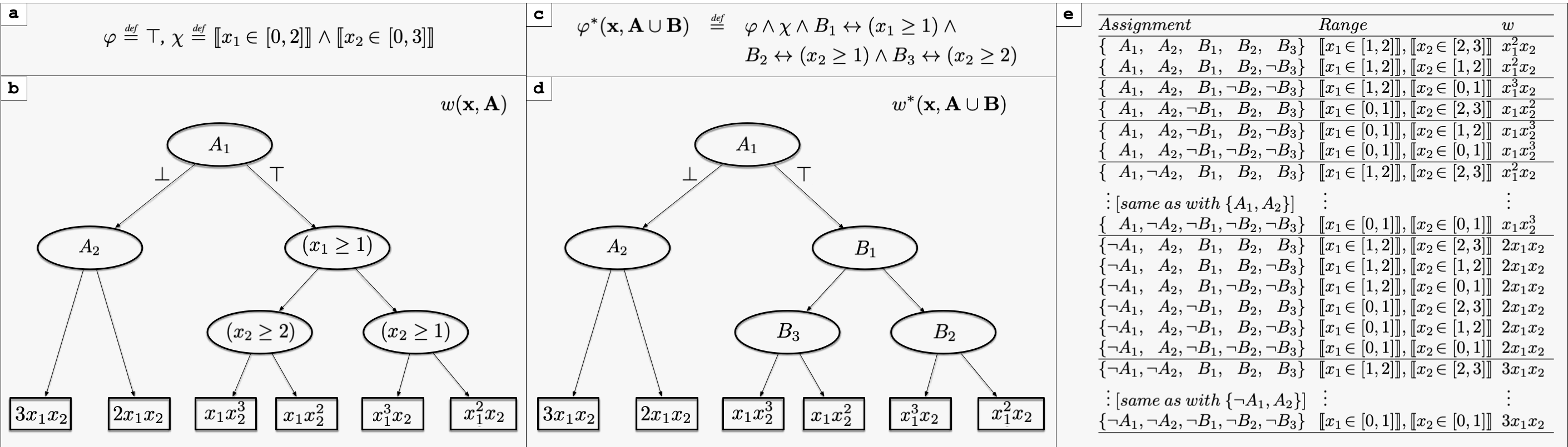
Figure 1: Example highlighting the efficiency issues of the WMI-PA algorithm. (a) definition of formula $\varphi$ (trivially true) and support $\chi$. (b) definition of the weight function $w(\mathbf{x},\mathbf{A})$. Round nodes indicate if-then-else conditions, with true and false cases on the right and left outgoing edges respectively. Squared nodes indicate ${\sf FI}^{\mathcal{LRA}}$ weight functions. (c) novel version of the formula $\varphi^{*}(\mathbf{x},\mathbf{A}\cup\mathbf{B})$ after the application of the LabelConditions(…) step of WMI-PA. (d) novel version of the weight function $w^{*}(\mathbf{x},\mathbf{A}\cup\mathbf{B})$, where all $\mathcal{LRA}$ conditions have been replaced with the fresh Boolean variables introduced in $\varphi^{*}(\mathbf{x},\mathbf{A}\cup\mathbf{B})$. (e) List of assignments obtained by WMI-PA on $\mathbf{A}\cup\mathbf{B}$. Notice the amount of assignments sharing the same ${\sf FI}^{\mathcal{LRA}}$ weight function.

Example 1

Let $\varphi\stackrel{{\scriptstyle\text{\tiny def}}}{{=}}\top$, $\chi\stackrel{{\scriptstyle\text{\tiny def}}}{{=}}\llbracket x_{1}\!\in[0,2]{}\rrbracket\wedge\llbracket x_{2}\!\in[0,3]{}\rrbracket$ (Figure 1(a)) and let $w(\mathbf{x},\mathbf{A})$ be a tree-structured weight function defined as in Figure 1(b). To compute ${\sf WMI}(\varphi\wedge\chi,w|\mathbf{x},\mathbf{A})$, six integrals have to be computed:

$x_{1}^{2}x_{2}$ on $\llbracket x_{1}\!\in[1,2]{}\rrbracket\wedge\llbracket x_{2}\!\in[1,3]{}\rrbracket$ (if $A_{1}=\top$)
$x_{1}^{3}x_{2}$ on $\llbracket x_{1}\!\in[1,2]{}\rrbracket\wedge\llbracket x_{2}\!\in[0,1]{}\rrbracket$ (if $A_{1}=\top$)
$x_{1}x_{2}^{2}$ on $\llbracket x_{1}\!\in[0,1]{}\rrbracket\wedge\llbracket x_{2}\!\in[2,3]{}\rrbracket$ (if $A_{1}=\top$)
$x_{1}x_{2}^{3}$ on $\llbracket x_{1}\!\in[0,1]{}\rrbracket\wedge\llbracket x_{2}\!\in[0,2]{}\rrbracket$ (if $A_{1}=\top$).
$2x_{1}x_{2}$ on $\llbracket x_{1}\!\in[0,2]{}\rrbracket\wedge\llbracket x_{2}\!\in[0,3]{}\rrbracket$ (if $A_{1}=\bot,A_{2}=\top$)
$3x_{1}x_{2}$ on $\llbracket x_{1}\!\in[0,2]{}\rrbracket\wedge\llbracket x_{2}\!\in[0,3]{}\rrbracket$ (if $A_{1}=\bot,A_{2}=\bot$)

When WMI-PA is used (Algorithm 1), applying LabelConditions(…) we obtain (Figure 1(c)):

$$\varphi^{*}(\mathbf{x},\mathbf{A}\cup\mathbf{B}) \stackrel{{\scriptstyle\text{\tiny def}}}{{=}} \varphi\wedge\chi\wedge B_{1}\leftrightarrow(x_{1}\geq 1)\wedge$$

$$B_{2}\leftrightarrow(x_{2}\geq 1)\wedge B_{3}\leftrightarrow(x_{2}\geq 2)$$

and the weight function $w^{*}(\mathbf{x},\mathbf{A}\cup\mathbf{B})$ shown in Figure 1(d). Then, by applying $\mathcal{T}\mathcal{T}\mathcal{A}({\sf PredAbs}_{[\varphi^{*}]}(\mathbf{A}^{*}))$ (row 2) we obtain 24 total assignments ${\mathcal{M}}^{\mathbf{A}^{*}}{}$ on $\mathbf{A}\cup\mathbf{B}$, as shown in Figure 1(e).. Notice that WMI-PA uselessly splits into 2 parts the integrals on $x_{1}^{2}x_{2}$ and $x_{1}x_{2}^{3}$ and into 6 parts the integral on $2x_{1}x_{2}$ and on $3x_{1}x_{2}$. Also, it repeats the very same integrals for $\{{A_{1},A_{2},...}\}$ and $\{{A_{1},\neg A_{2},...}\}$. $\diamond$

We highlight two facts. First, WMI-PA enumerates total truth assignments on the Boolean atoms $\mathbf{A}\cup\mathbf{B}$ in $\mathcal{T}\mathcal{T}\mathcal{A}(\exists\mathbf{x}.\varphi^{*})$ (6) (row 2 in Algorithm 1), assigning also unnecessary values. Second, WMI-PA labels $\mathcal{LRA}$ conditions in $w$ by means of fresh Boolean atoms $\mathbf{B}$ (row 1 in Algorithm 1). This forces the enumerator to assign all their values in every assignment, even when not necessary.

The key issue about WMI-PA is that the enumeration of $\mathcal{T}\mathcal{T}\mathcal{A}(\exists\mathbf{x}.\varphi^{*})$ in (6) and of $\mathcal{T}\mathcal{A}(\varphi^{*}_{[\mu^{\mathbf{A}^{*}}]})$ in (4) (rows 2 and 11 in Algorithm 1) is not aware of the conditional structure of the weight function $w$, in particular, it is not aware of the fact that often partial assignments to the set of conditions in $w^{*}$ (both Boolean and $\mathcal{LRA}$) are sufficient to identify the value of a ${\sf FIUC}^{\mathcal{LRA}}$ function (e.g $\{{A_{1},B_{1},B_{2}}\}$ suffices to identify $x_{1}^{2}x_{2}$, or $\{{\neg A_{1},A_{2}}\}$ suffices to identify $2x_{1}x_{2}$), so that it is forced to enumerate all total assignments extending them (e.g. $\{{A_{1},A_{2},B_{1},B_{2},B_{3}}\}$ and $\{{A_{1},A_{2},B_{1},B_{2},\neg B_{3}}\}$).

Thus, to cope with this issue, we need to modify WMI-PA to make it aware of the conditional structure of $w$.

4 Making WMI-PA Weight-Structure Aware

The key idea to prevent total enumeration works as follows. We do not rename with $\mathbf{B}$ the conditions $\mathbf{\Psi}$ in $w$ and, rather than enumerating total truth assignments for $\exists\mathbf{x}.\varphi^{*}$ as in (6)–(7), we enumerate partial assignments for $\exists\mathbf{x}.\varphi^{**}$ where $\varphi^{**}\stackrel{{\scriptstyle\text{\tiny def}}}{{=}}\varphi\wedge\chi\wedge{\sf sk}(w)$ and ${\sf sk}(w)$ –which we call the conditional skeleton of $w$– is a $\mathcal{LRA}$ formula s.t.:
$(a)$ its atoms are all and only the conditions in $\mathbf{\Psi}$,
$(b)$ is $\mathcal{LRA}$-valid, so that $\varphi\wedge\chi$ is equivalent to $\varphi\wedge\chi\wedge{\sf sk}(w)$,
$(c)$ any partial truth value assignment $\mu$ to the conditions $\mathbf{\Psi}$ which makes ${\sf sk}(w)$ true is such that $w_{[\mu]}$ is ${\sf FI}^{\mathcal{LRA}}$.
Thus, we have that (2) can be rewritten as:

$${\sf WMI}(\varphi,w|\mathbf{x},\mathbf{A}) = \sum_{\mu\in\mathcal{T}\mathcal{A}(\exists\mathbf{x}.\varphi^{**})}2^{|\mathbf{A}\setminus\mu|}\cdot{\sf WMI_{nb}}(\varphi^{**}_{[\mu]},w_{[\mu]}|\mathbf{x})$$ (9)

$$\varphi^{**} \stackrel{{\scriptstyle\text{\tiny def}}}{{=}} \varphi\wedge\chi\wedge{\sf sk}(w)$$ (10)

where $|\mathbf{A}\setminus\mu|$ is the number of Boolean atoms in $\mathbf{A}$ that are not assigned by $\mu$. Condition $(c)$ guarantees that ${\sf WMI_{nb}}(\varphi^{**}_{[\mu]},w_{[\mu]}|\mathbf{x})$ in (9) can be directly computed, without further partitioning. The $2^{|\mathbf{A}\setminus\mu|}$ factor in (9) resembles the fact that, if some Boolean atom $A_{i}\in\mathbf{A}$ is not assigned in $\mu$, then ${\sf WMI_{nb}}(\varphi^{**}_{[\mu]},w_{[\mu]}|\mathbf{x})$ should be counted twice because $\mu$ represents two assignments $\mu\cup\{{A_{i}}\}$ and $\mu\cup\{{\neg A_{i}}\}$ which would produce two identical integrals.

Notice that logic-wise ${\sf sk}(w)$ is non-informative because it is a valid formula. Nevertheless, the role of ${\sf sk}(w)$ is to mimic the structure of $w$ so that to “make the enumerator aware of the presence of the conditions $\mathbf{\Psi}{}$”, forcing every assignment $\mu$ to assign truth values also to these conditions which are necessary to make $w_{[\mu]}$ ${\sf FI}^{\mathcal{LRA}}$ and hence make ${\sf WMI_{nb}}(\varphi^{**}_{[\mu]},w_{[\mu]}|\mathbf{x})$ directly computable, without further partitioning.

An important issue is to avoid ${\sf sk}(w)$ blow up in size. E.g., one could use as ${\sf sk}(w)$ a formula encoding the conditional structure of an XADDs or (F)XSDDs, but this may cause a blow up in size, as discussed in Section 3.1.

In order to prevent such problems, we do not generate ${\sf sk}(w)$ explicitly. Rather, we build it as a disjunction of partial assignments over $\mathbf{\Psi}$ which we enumerate progressively. To this extent, we define ${\sf sk}(w)\stackrel{{\scriptstyle\text{\tiny def}}}{{=}}\exists\mathbf{y}.\llbracket y=w\rrbracket{}$ where $\llbracket y=w\rrbracket$ is a formula on $\mathbf{A}$,$\mathbf{x}$,$\mathbf{y}$ s.t. $\mathbf{y}\stackrel{{\scriptstyle\text{\tiny def}}}{{=}}\{{y,y_{1},...,y_{k}}\}$ is a set of fresh variables. Thus, $\mathcal{T}\mathcal{A}(\exists\mathbf{x}.(\varphi\wedge\chi\wedge\exists\mathbf{y}.\llbracket y=w\rrbracket{}))$ can be computed as $\mathcal{T}\mathcal{A}(\exists\mathbf{x}\mathbf{y}.(\varphi\wedge\chi\wedge\llbracket y=w\rrbracket{}))$ because the $\mathbf{y}$’s do not occur in $\varphi\wedge\chi$, with no need to generate ${\sf sk}(w)$ explicitly. The enumeration of $\mathcal{T}\mathcal{A}(\exists\mathbf{x}\mathbf{y}.(\varphi\wedge\chi\wedge\llbracket y=w\rrbracket{}))$ is performed by the very same SMT-based procedure used in Morettin et al. [2019].

$\llbracket y=w\rrbracket$ is obtained by taking $(y=w)$, s.t. $y$ is fresh, and recursively substituting bottom-up every conditional term $({\sf If}\ \psi_{i}\ {\sf Then}\ t_{i1}\ {\sf Else}\ {t_{i2}})$ in it with a fresh variable $y_{i}\in\mathbf{y}$, adding the definition of $(y_{i}=({\sf If}\ \psi_{i}\ {\sf Then}\ t_{i1}\ {\sf Else}\ {t_{i2}}))$ as

$$(\neg\psi_{i}\vee y_{i}=t_{i1})\wedge(\psi_{i}\vee y_{i}=t_{i2}).$$ (11)

This labeling&rewriting process, which is inspired to labeling CNF-ization [Tseitin, 1968], guarantees that the size of $\llbracket y=w\rrbracket$ is linear wrt. that of $w$. E.g., if (8) holds, then $\llbracket y=w\rrbracket$ is $(y=\prod_{i=1}^{N}y_{i})\wedge\bigwedge_{i=1}^{N}((\neg\psi_{i}\vee y_{i}=w_{i1}(\mathbf{x}))\wedge(\psi_{i}\vee y_{i}=w_{i2}(\mathbf{x})))$.

One problem with the above definition of $\llbracket y=w\rrbracket$ is that it is not a $\mathcal{LRA}$-formula, because $w$ may include multiplications or even transcendental functions out of the conditions $\mathbf{\Psi}$ , which makes SMT reasoning over it dramatically hard or even undecidable. We notice, however, that when computing $\mathcal{T}\mathcal{A}(\exists\mathbf{x}\mathbf{y}.(\varphi\wedge\chi\wedge\llbracket y=w\rrbracket{}))$ the arithmetical functions (including operators $+,-,*,/$) occurring in $w$ out of the conditions $\mathbf{\Psi}$ have no role, since the only fact that we need to guarantee for the validity of ${\sf sk}(w)$ is that they are indeed functions, so that $\exists y.(y=f(...))$ is always valid. (In substance, during the enumeration we are interested only in the truth values of the conditions $\mathbf{\Psi}$ in $\mu$ which make $w_{[\mu]}$ ${\sf FI}^{\mathcal{LRA}}$, regardless the actual values of $w_{[\mu]}$). Therefore we can safely substitute condition-less arithmetical functions (including operators $+,-,\cdot,/$) with some fresh uninterpreted function symbols, obtaining a $\mathcal{LRA}\cup\mathcal{EUF}$-formula $\llbracket y=w\rrbracket_{\mathcal{EUF}}$, which is relatively easy to solve by standard SMT solvers [Barrett et al., 2009]. It is easy to see that a partial assignment $\mu$ evaluating $\llbracket y=w\rrbracket$ to true is $\mathcal{LRA}$-satisfiable iff its corresponding assignment $\mu_{\mathcal{EUF}}$ is $\mathcal{LRA}\cup\mathcal{EUF}$-satisfiable. Therefore, we can modify the enumeration procedure into $\mathcal{T}\mathcal{A}(\exists\mathbf{x}\mathbf{y}.(\varphi\wedge\chi\wedge\llbracket y=w\rrbracket_{\mathcal{EUF}}{}))$.

Finally, we enforce the fact that the two branches of an if-then-else are alternative by adding to (11) a mutual-exclusion constraint $\neg(y_{i}=t_{i1})\vee\neg(y_{i}=t_{i2})$, so that the choice of the function is univocally associated to the list of decisions on the $\psi_{i}$s. The procedure producing $\llbracket y=w\rrbracket_{\mathcal{EUF}}$ is described in detail in Appendix, Algorithm 1.

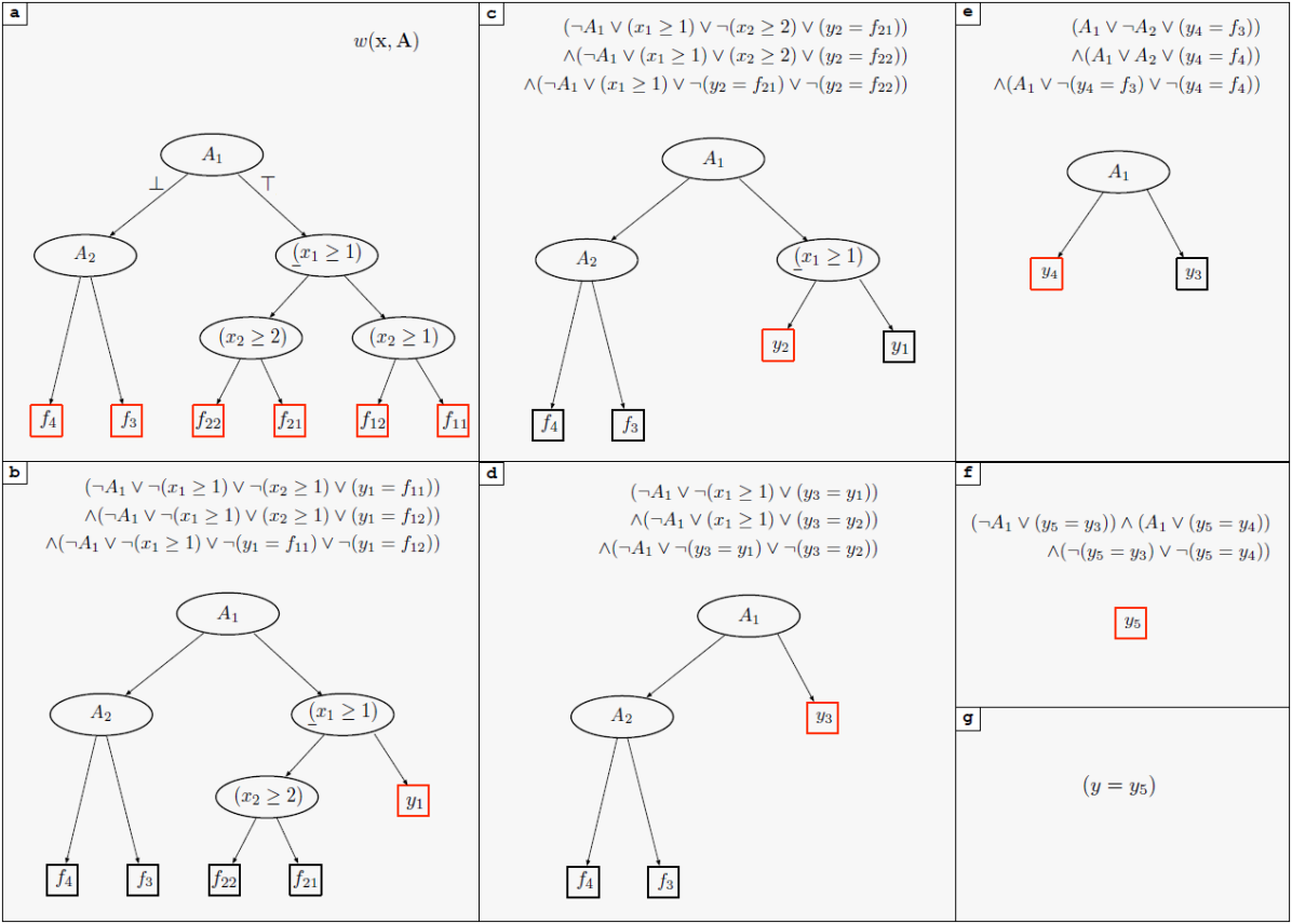
Figure 2: Example of bottom-up procedure for computing the relabeling function $\llbracket y=w\rrbracket_{\mathcal{EUF}}$. (a) Replacement of ${\sf FI}^{\mathcal{LRA}}$ weight functions (the leaves of the tree, highlighted in red) with $\mathcal{EUF}$ function symbols (we dropped the dependency on $x$ for compactness). (b-g) Sequence of relabeling steps. At each step, a conditional term is replaced by a fresh $\mathcal{LRA}$ variable $y_{i}$. The encoding of the variable in shown in the upper part, while the lower part shows the weight function with the branch of the conditional term replaced with $y_{i}$ (highlighted in red). The last step consists in renaming the top variable as $y$, so that $y=w(\mathbf{x},\mathbf{A}){}$. The relabeling function $\llbracket y=w\rrbracket_{\mathcal{EUF}}$ is simply the conjunction of the encodings in the different steps.

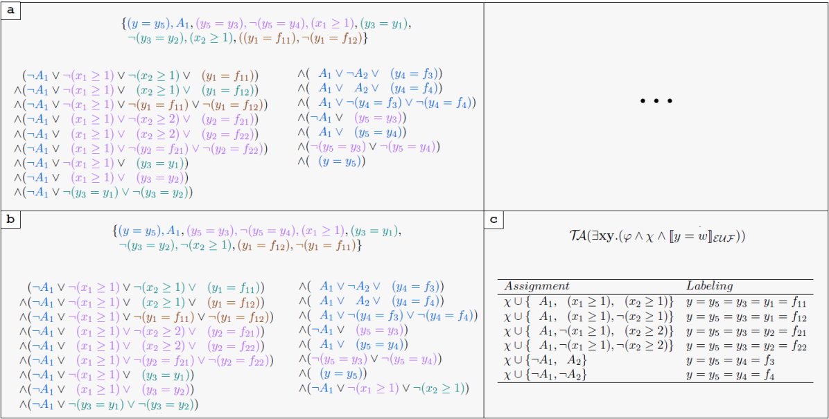
Figure 3: Example of structure-aware enumeration performed by SA-WMI-PA on the problem in Example 1. (a) Generation of the first assignment. The assignment is on top, while the bottom part shows the $\llbracket y=w\rrbracket_{\mathcal{EUF}}$ formula. Colors indicate the progression of the generation, in terms of atoms added (top) and parts of the formula to be removed as a consequence (bottom). For the sake of simplicity all atoms until the next atom in $\Psi\stackrel{{\scriptstyle\text{\tiny def}}}{{=}}\{{A_{1},A_{2},(x_{1}\geq 1),(x_{2}\geq 1),(x_{2}\geq 2)}\}$ (if any) are given the same color. (b) Generation of the second assignment. Note how the $\llbracket y=w\rrbracket_{\mathcal{EUF}}$ formula is enriched with the blocking clause $\neg A_{1}\vee\neg(x_{1}\geq 1)\vee\neg(x_{2}\geq 1)$ preventing the first assignment to be generated again. (c) Final result of the enumeration (which contains six assignments in total). The partial assignments are obtained by restricting the generated assignments on the conditions in $\Psi$ (and combining them with the atoms of $\chi$, which here are assigned deterministically.). For each assignment, the corresponding chain of equivalences of the $\mathbf{y}$s with the identified leaf ${\sf FI}^{\mathcal{LRA}}$ function is displayed.

Example 2

Consider the problem in Example 1. Figure 2 shows the relabeling process applied to the weight function $w$. The resulting $\llbracket y=w\rrbracket_{\mathcal{EUF}}$ formula is:

$\begin{array}[]{ll}\phantom{\wedge}\llbracket y=w\rrbracket(\mathbf{x}\cup\mathbf{y},\mathbf{A}){}\stackrel{{\scriptstyle\text{\tiny def}}}{{=}}\\ \phantom{\wedge}(\neg A_{1}\vee\neg(x_{1}\geq 1)\vee\neg(x_{2}\geq 1)&\vee\phantom{\neg}(y_{1}=f_{11}(\mathbf{x})))\\ \wedge(\neg A_{1}\vee\neg(x_{1}\geq 1)\vee\phantom{\neg}(x_{2}\geq 1)&\vee\phantom{\neg}(y_{1}=f_{12}(\mathbf{x})))\\ \wedge(\neg A_{1}\vee\neg(x_{1}\geq 1)\vee\neg(y_{1}=f_{11}(\mathbf{x}))&\vee\neg(y_{1}=f_{12}(\mathbf{x})))\\ \wedge(\neg A_{1}\vee\phantom{\neg}(x_{1}\geq 1)\vee\neg(x_{2}\geq 2)&\vee\phantom{\neg}(y_{2}=f_{21}(\mathbf{x})))\\ \wedge(\neg A_{1}\vee\phantom{\neg}(x_{1}\geq 1)\vee\phantom{\neg}(x_{2}\geq 2)&\vee\phantom{\neg}(y_{2}=f_{22}(\mathbf{x})))\\ \wedge(\neg A_{1}\vee\phantom{\neg}(x_{1}\geq 1)\vee\neg(y_{2}=f_{21}(\mathbf{x}))&\vee\neg(y_{2}=f_{22}(\mathbf{x})))\\ \wedge(\neg A_{1}\vee\neg(x_{1}\geq 1)&\vee\phantom{\neg}(y_{3}=y_{1}))\\ \wedge(\neg A_{1}\vee\phantom{\neg}(x_{1}\geq 1)&\vee\phantom{\neg}(y_{3}=y_{2}))\\ \wedge(\neg A_{1}\vee\neg(y_{3}=y_{1})\vee\neg(y_{3}=y_{2}))&\\ \wedge(\phantom{\neg}A_{1}\vee\neg A_{2}&\vee\phantom{\neg}(y_{4}=f_{3}(\mathbf{x})))\\ \wedge(\phantom{\neg}A_{1}\vee\phantom{\neg}A_{2}&\vee\phantom{\neg}(y_{4}=f_{4}(\mathbf{x})))\\ \wedge(\phantom{\neg}A_{1}\vee\neg(y_{4}=f_{3}(\mathbf{x}))\vee\neg(y_{4}=f_{4}(\mathbf{x})))&\\ \wedge(\neg A_{1}&\vee\phantom{\neg}(y_{5}=y_{3}))\\ \wedge(\phantom{\neg}A_{1}&\vee\phantom{\neg}(y_{5}=y_{4}))\\ \wedge(\neg(y_{5}=y_{3})\vee\neg(y_{5}=y_{4}))&\\ \wedge(\phantom{\neg}(y=y_{5}))&\\ \end{array}$

Figure 3 illustrates a possible enumeration process. The algorithm enumerates partial assignments satisfying $\varphi\wedge\chi\wedge\llbracket y=w\rrbracket_{\mathcal{EUF}}{}$, restricted on the conditions $\Psi\stackrel{{\scriptstyle\text{\tiny def}}}{{=}}\{{A_{1},A_{2},(x_{1}\geq 1),(x_{2}\geq 1),(x_{2}\geq 2)}\}$, which is equivalent to enumerate $\mathcal{T}\mathcal{A}(\exists\mathbf{x}\mathbf{y}.(\varphi\wedge\chi\wedge\llbracket y=w\rrbracket_{\mathcal{EUF}}{}))$. Assuming the enumeration procedure picks nondeterministic choices following the order of the above set  and assigning positive values first, then in the first branch the following satisfying partial assignment is generated, in order: $\begin{array}[]{l}\chi\cup\{(y=y_{5}),\underline{A_{1}},(y_{5}=y_{3}),\neg(y_{5}=y_{4}),\underline{(x_{1}\geq 1)},\\ (y_{3}=y_{1}),\neg(y_{3}=y_{2}),\underline{(x_{2}\geq 1)},(y_{1}=f_{11}(\mathbf{x})),\\ \neg(y_{1}=f_{12}(\mathbf{x}))\}.\end{array}$

(Notice that, following the chains of true equalities, we have $y=y_{5}=y_{3}=y_{1}=f_{11}(\mathbf{x})$.) Then the SMT solver extracts from it the subset $\{{A_{1},(x_{1}\geq 1),(x_{2}\geq 1)}\}$ restricted on the conditions in $\Psi$. Then the blocking clause $\neg A_{1}\vee\neg(x_{1}\geq 1)\vee\neg(x_{2}\geq 1)$ is added to the formula, which prevents to enumerate the same subset again. This forces the algorithm to backtrack and generate $\begin{array}[]{l}\chi\cup\{(y=y_{5}),\underline{A_{1}},(y_{5}=y_{3}),\neg(y_{5}=y_{4}),(x_{1}\geq 1),\\ (y_{3}=y_{1}),\neg(y_{3}=y_{2}),{\neg(x_{2}\geq 1)},(y_{1}=f_{12}(\mathbf{x})),\\ \neg(y_{1}=f_{11}(\mathbf{x}))\}.\end{array}$ producing the assignment: $\{{A_{1},(x_{1}\geq 1),\neg(x_{2}\geq 1)}\}$. 

Overall, the algorithm enumerates the following ordered collection of partial assignments restricted to $Atoms(\varphi\wedge\chi)\cup\mathbf{\Psi}$:
$\begin{array}[]{ll}\chi\cup\{{\phantom{\neg}A_{1},\phantom{\neg}(x_{1}\geq 1),\phantom{\neg}(x_{2}\geq 1)}\},&//y=...=f_{11}(\mathbf{x})\\ \chi\cup\{{\phantom{\neg}A_{1},\phantom{\neg}(x_{1}\geq 1),\neg(x_{2}\geq 1)}\},&//y=...=f_{12}(\mathbf{x})\\ \chi\cup\{{\phantom{\neg}A_{1},\neg(x_{1}\geq 1),\phantom{\neg}(x_{2}\geq 2)}\},&//y=...=f_{21}(\mathbf{x})\\ \chi\cup\{{\phantom{\neg}A_{1},\neg(x_{1}\geq 1),\neg(x_{2}\geq 2)}\},&//y=...=f_{22}(\mathbf{x})\\ \chi\cup\{{\neg A_{1},\phantom{\neg}A_{2}}\},&//y=...=f_{3}(\mathbf{x})\\ \chi\cup\{{\neg A_{1},\neg A_{2}}\}&//y=...=f_{4}(\mathbf{x})\\ \end{array}$

which correspond to the six integrals of Example 1. Notice that according to (2) the first four integrals have to be multiplied by 2, because the partial assignment $\{{A_{1}}\}$ covers two total assignments $\{{A_{1},A_{2}}\}$ and $\{{A_{1},\neg A_{2}}\}$. Notice also that the disjunction of the six partial assignments,
$(A_{1}\wedge(x_{1}\geq 1)\wedge(x_{2}\geq 1))\vee...\vee(\neg A_{1}\wedge\neg A_{2}),$ matches the definition of ${\sf sk}(w)$, which we have computed by progressive enumeration rather than encoded a priori. $\diamond$

Based on the previous ideas, we develop SA-WMI-PA, a novel “weight structure aware” variant of WMI-PA. The pseudocode of SA-WMI-PA is reported in Algorithm  2.

As with WMI-PA, we enumerate the assignments in two main steps: in the first loop (rows 3:-7:) we generate a set ${\mathcal{M}}^{\mathbf{A}^{*}}{}$ of partial assignments $\mu^{\mathbf{A}^{*}}$ over the Boolean variables $\mathbf{A}$, s.t. $\varphi^{**}_{[\mu^{\mathbf{A}}]}$ is $\mathcal{LRA}$-satisfiable and does not contain Boolean variables anymore. In Example 2 ${\mathcal{M}}^{\mathbf{A}^{*}}{}\stackrel{{\scriptstyle\text{\tiny def}}}{{=}}\{{\{{A_{1}}\},\{{\neg A_{1},A_{2}}\},\{{\neg A_{1},\neg A_{2}}\}}\}$. In the second loop (rows 11:-11:), for each $\mu^{\mathbf{A}^{*}}$ in ${\mathcal{M}}^{\mathbf{A}^{*}}{}$ we enumerate the set ${\mathcal{M}}^{\mathcal{LRA}}$ of $\mathcal{LRA}$-satisfiable partial assignments satisfying $\varphi^{**}_{[\mu^{\mathbf{A}^{*}}]}$ (that is, on $\mathcal{LRA}$ atoms in $Atoms(\varphi\wedge\chi)\cup\mathbf{\Psi}$), we compute the integral ${\sf WMI_{nb}}(\mu^{\mathcal{LRA}},w_{[\mu^{\mathbf{A}}*]}|\mathbf{x})$, multiply it by the $2^{|\mathbf{A}\setminus\mu^{\mathbf{A}^{*}}|}$ factor and add it to the result. In Example 2, if e.g. $\mu^{\mathbf{A}^{*}}{}=\{{A_{1}}\}$, $\mathcal{T}\mathcal{A}({\sf PredAbs}_{[\varphi^{**}_{[\mu^{\mathbf{A}^{*}}]}]}(Atoms(\varphi^{**}_{[\mu^{\mathbf{A}^{*}}]})))$ computes the four partial assignments $\{\chi\cup\{{(x_{1}\geq 1),(x_{2}\geq 1)}\},...,\chi\cup\{{\neg(x_{1}\geq 1),\neg(x_{2}\geq 2)}\}\}$.

Algorithm 2 SA-WMI-PA($\varphi$, $w$, $\mathbf{x}$, $\mathbf{A}$)

• ${\mathcal{M}}^{\mathbf{A}^{*}}\leftarrow\emptyset;vol\leftarrow 0$

• $\varphi^{**}\leftarrow\varphi\wedge\chi\wedge\llbracket y=w\rrbracket_{\mathcal{EUF}}{}$

• ${\mathcal{M}}^{\mathbf{A}}\leftarrow\mathcal{T}\mathcal{A}({\sf PredAbs}_{[\varphi^{**}]}(\mathbf{A}))$

• for $\mu^{\mathbf{A}}\in{\mathcal{M}}^{\mathbf{A}}$ do

  • ${\sf Simplify}(\varphi^{**}_{[\mu^{\mathbf{A}}]})$

  • if $\varphi^{**}_{[\mu^{\mathbf{A}}]}$ does not contain Boolean variables then

    • ${\mathcal{M}}^{\mathbf{A}^{*}}\leftarrow{\mathcal{M}}^{\mathbf{A}^{*}}\cup\{{\mu^{\mathbf{A}}}\}$

  • else

    • for $\mu^{\mathbf{A}}_{residual}\in\mathcal{T}\mathcal{T}\mathcal{A}({\sf PredAbs}_{[\varphi^{**}_{[\mu^{\mathbf{A}}]}]}(\mathbf{A}))$ do

      • ${\mathcal{M}}^{\mathbf{A}^{*}}\leftarrow{\mathcal{M}}^{\mathbf{A}^{*}}\cup\{{\mu^{\mathbf{A}}\wedge\mu^{\mathbf{A}}_{residual}}\}$

• for $\mu^{\mathbf{A}^{*}}\in{\mathcal{M}}^{\mathbf{A}^{*}}$ do

  • $k\leftarrow|\mathbf{A}\setminus\mu^{\mathbf{A}^{*}}|$

  • ${\sf Simplify}(\varphi^{**}_{[\mu^{\mathbf{A}^{*}}]})$

  • if ${\sf LiteralConjunction}(\varphi^{**}_{[\mu^{\mathbf{A}^{*}}]})$ then

    • $vol\leftarrow vol+2^{k}\cdot{\sf WMI_{nb}}(\varphi^{**}_{[\mu^{\mathbf{A}^{*}}]},w_{[\mu^{\mathbf{A}}*]}|\mathbf{x})$

  • else

    • ${\mathcal{M}}^{\mathcal{LRA}}\leftarrow\mathcal{T}\mathcal{A}({\sf PredAbs}_{[\varphi^{**}_{[\mu^{\mathbf{A}^{*}}]}]}(Atoms(\varphi^{**}_{[\mu^{\mathbf{A}^{*}}]})))$

    • for $\mu^{\mathcal{LRA}}\in{\mathcal{M}}^{\mathcal{LRA}}$ do

      • $vol\leftarrow vol+2^{k}\cdot{\sf WMI_{nb}}(\mu^{\mathcal{LRA}},w_{[\mu^{\mathbf{A}}*]}|\mathbf{x})$

• return $vol$

In detail, in row 2: we extend $\varphi\wedge\chi$ with $\llbracket y=w\rrbracket_{\mathcal{EUF}}{}$ to provide structure awareness. (We recall that, unlike with WMI-PA, we do not label $\mathcal{LRA}$ conditions with fresh Boolean variables $\mathbf{B}{}$.) Next, in row 3: we perform $\mathcal{T}\mathcal{A}({\sf PredAbs}_{[\varphi^{**}_{[\mu^{\mathbf{A}}]}]}(\mathbf{A}))$ to obtain a set ${\mathcal{M}}^{\mathbf{A}}{}$ of partial assignments restricted on Boolean atoms $\mathbf{A}$. Then, for each assignment $\mu^{\mathbf{A}}\in{\mathcal{M}}^{\mathbf{A}}$ we build the (simplified) residual $\varphi^{**}_{[\mu^{\mathbf{A}}]}$. Since $\mu^{\mathbf{A}}$ is partial, $\varphi^{**}_{[\mu^{\mathbf{A}}]}$ is not guaranteed to be free of Boolean variables $\mathbf{A}$, as shown in Example 3. If this is the case, we simply add $\mu^{\mathbf{A}}$ to ${\mathcal{M}}^{\mathbf{A}^{*}}$, otherwise we invoke $\mathcal{T}\mathcal{T}\mathcal{A}({\sf PredAbs}_{[\varphi^{**}_{[\mu^{\mathbf{A}}]}]}(\mathbf{A}))$ to assign the remaining variables and conjoin each assignment $\mu^{\mathbf{A}}_{residual}$ to $\mu^{\mathbf{A}}$, ensuring that the residual now contains only $\mathcal{LRA}$ atoms (rows 4:- 4:). The second loop (rows 11:-11:) resembles the main loop in WMI-PA, with the only relevant difference that, since $\mu^{\mathbf{A}^{*}}$ is partial, the integral is multiplied by a $2^{|\mathbf{A}\setminus\mu^{\mathbf{A}^{*}}|}$ factor.

Notice that in general the assignments $\mu^{\mathbf{A}^{*}}$ are partial even if the steps in rows 9:-10: are executed; the set of residual Boolean variables in $\varphi^{**}_{[\mu^{\mathbf{A}}]}$ are a (possibly much smaller) subset of $\mathbf{A}\setminus\mu^{\mathbf{A}}$ because some of them do not occur anymore in $\varphi^{**}_{[\mu^{\mathbf{A}}]}$ after the simplification, as shown in the following example.

Example 3

Let $\varphi\stackrel{{\scriptstyle\text{\tiny def}}}{{=}}(A_{1}\vee A_{2}\vee A_{3})\wedge(\neg A_{1}\vee A_{2}\vee(x\geq 1))\wedge(\neg A_{2}\vee(x\geq 2))\wedge(\neg A_{3}\vee(x\leq 3))$, $\chi\stackrel{{\scriptstyle\text{\tiny def}}}{{=}}\llbracket x_{1}\!\in[0,4]{}\rrbracket$ and $w(\mathbf{x},\mathbf{A})\stackrel{{\scriptstyle\text{\tiny def}}}{{=}}1.0$. Suppose $\mathcal{T}\mathcal{A}({\sf PredAbs}_{[\varphi^{**}]}(\mathbf{A}))$ finds the partial assignment $\{{(x\geq 0),(x\leq 4),A_{2},(x\geq 1),(x\geq 2),(x\leq 3)}\}$, whose projected version is $\mu^{\mathbf{A}}\stackrel{{\scriptstyle\text{\tiny def}}}{{=}}\{{A_{2}}\}$ (row 3:). Then $\varphi^{**}_{[\mu^{\mathbf{A}}]}$ reduces to $(\neg A_{3}\vee(x\leq 3))$, so that ${\mathcal{M}}^{\mathbf{A}^{*}}$ is $\{{\{{A_{2},A_{3}}\},\{{A_{2},\neg A_{3}}\}}\}$, avoiding branching on $A_{1}$. $\diamond$

We stress the fact that in our actual implementation, like with that of WMI-PA, the potentially-large sets ${\mathcal{M}}^{\mathbf{A}^{*}}$ and ${\mathcal{M}}^{\mathcal{LRA}}$ are not generated explicitly. Rather, their elements are generated, integrated and then dropped one-by-one, so that to avoid space blowup.

We highlight two main differences wrt. WMI-PA. First, unlike with WMI-PA, the generated assignments $\mu^{\mathbf{A}}$ on $\mathbf{A}$ are partial, each representing $2^{|\mathbf{A}\setminus\mu^{\mathbf{A}}|}$ total ones. Second, the assignments on (non-Boolean) conditions $\mathbf{\Psi}$ inside the $\mu^{\mathcal{LRA}}$s are also partial, whereas with WMI-PA the assignments to the $\mathbf{B}$s are total. This may drastically reduce the number of integrals to compute, as empirically demonstrated in the next section.

5 Experimental Evaluation

The novel algorithm SA-WMI-PA is compared to the original WMI-PA algorithm [Morettin et al., 2019], and the WMI solvers based on KC: XADD [Kolb et al., 2018], XSDD and FXSDD [Kolb et al., 2020]. Each of these methods is called from the Python framework pywmi [Kolb et al., 2019]. For both WMI-PA and SA-WMI-PA, we use MathSAT for SMT enumeration and LattE Integrale for computing integrals. For the KC algorithms we use PSiPSI [Gehr et al., 2016] as symbolic computer algebra backend. All experiments are performed on an Intel Xeon Gold 6238R @ 2.20GHz 28 Core machine with 128GB of ram and running Ubuntu Linux 20.04. The code of SA-WMI-PA is freely available at https://github.com/unitn-sml/wmi-pa.
For improved readability, in both the experiments we report runtime using cactus plots, i.e. the single problem instances are increasingly sorted by runtime for each algorithm separately. We highlight how, by construction, problem instances of the same tick of the x-axis are not guaranteed to be the same for different algorithms. Steeper slopes of an algorithm curve means less efficiency.

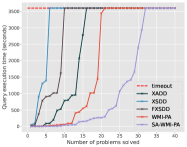
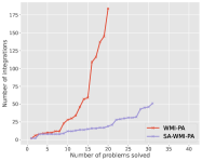
Figure 4: Cactus plots reporting execution time for all methods on the synthetic experiments (left); number of integrals (right) for WMI-PA and SA-WMI-PA.

5.1 Synthetic experiments

We first evaluate our algorithm on random formulas and weights, following the experimental protocol of Morettin et al. [2019]. We define two recursive procedures to generate $\mathcal{LRA}$ formulae and weight functions with respect to a positive integer number $D$, named depth:

$${\sf r}_{\varphi}(D)= \begin{cases}\bigoplus_{q=1}^{Q}{\sf r}_{\varphi}(D-1)\hskip 65.44142pt\text{ if }D>0\\ [\neg]A^{\mathbb{B}/\mathbb{R}}\hskip 101.00737pt\text{ otherwise}\\ \end{cases}$$

$${\sf r}_{w}(D)= \begin{cases}\begin{cases}\llbracket{\sf If}\ {\sf r}_{\varphi}(D)\ {\sf Then}\ {\sf r}_{w}(D-1)\ {\sf Else}\ {\sf r}_{w}(D-1){}\rrbracket&\\ \text{or}\\ {\sf r}_{w}(D-1)\otimes{\sf r}_{w}(D-1)\ \ \ \ \ \ \ \ \ \ \ \text{ if }D>0\\ \end{cases}\\ P_{\sf random}(\mathbf{x})\hskip 91.04872pt\text{ otherwise}\end{cases}$$

where $\bigoplus\in\{\bigvee,\bigwedge,\neg\bigvee,\neg\bigwedge\}$, $\otimes\in\{+,\cdot\}$ and $P_{\sf random}(\mathbf{x})$ is a random polynomial function. Using these procedure we generate instances of synthetic problems:

$$\chi(\mathbf{x},\mathbf{A}) = {\sf r}_{\varphi}(D)\wedge\bigwedge_{x\in\mathbf{x}}\llbracket x\!\in[l_{x},u_{x}]{}\rrbracket$$

$$w(\mathbf{x},\mathbf{A}) = {\sf r}_{w}(D)$$

$$\varphi_{{\sf query}}(\mathbf{x},\mathbf{A}) = {\sf r}_{\varphi}(D)$$

where $l_{x},u_{x}$ are real numbers such that $\forall x.(l_{x}<u_{x})$.

In contrast with the benchmarks used in other recent works [Kolb et al., 2018, 2020], the procedure is not strongly biased towards the generation of problems with structural regularities, offering a more neutral perspective on how the different techniques are expected to perform in the wild. The generated synthetic benchmark contains problems where the number of both Boolean and real variables is set to 3, while the depth of weights functions fits in the range $[4,7]$. Timeout was set to 3600 seconds, similarly to what has been done in previous works.

In this settings, the approaches based on a SMT oracle clearly outperform those based on KC (Fig. 4 left). In addition, SA-WMI-PA greatly improves over WMI-PA, thanks to a drastic reduction in the number of integrals computed (Fig. 4 right), with the advantage of our approach getting more evident when the weight functions are deeper.

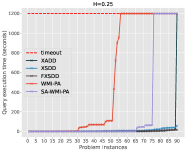
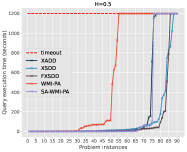
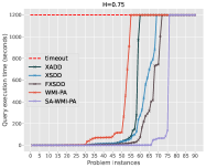
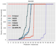
Figure 5: Cactus plots representing average query execution times and standard deviation in seconds on a set of DET problems with $H\in\{0.25,0.5,0.75,1\}$.

5.2 Density Estimation Trees

We explore the use of WMI solvers for marginal inference in real-world probabilistic models. In particular, we considered Density Estimation Trees (DETs) [Ram and Gray, 2011], hybrid density estimators encoding piecewise constant distributions. Having only univariate conditions in the internal nodes, DETs natively support tractable inference when single variables are considered. Answering queries like $Pr(X\leq Y)$ requires instead marginalizing over an oblique constraint, which is reduced to WMI: $Pr(X\leq Y)=\frac{WMI((X\leq Y)\wedge\chi_{DET},w_{DET})}{WMI(\chi_{DET},w_{DET})}$. Being able to address this type of queries is crucial to apply WMI-based inference to e.g. probabilistic formal verification tasks, involving constraints that the system should satisfy with high probability.

We considered a selection of hybrid datasets from the UCI repository [Dua and Graff, 2017], reported in Table 1 in the Appendix. Following the approach of Morettin et al. [2020], discrete numerical features were relaxed into continuous variables, while $n$-ary categorical features are one-hot encoded with $n$ binary variables.

After learning a DET on each dataset, we generated a benchmark of increasingly complex queries, 5 for each dataset, involving a ratio $H\in[0,1]$ of the continuous variables. More specifically, the queries are linear inequalities involving a number of variables $k=max(1,\lfloor H\cdot|\mathbf{x}|\rfloor)$. Figure 5 depicts the runtime of the algorithms for $H\in\{0.25,0.5,0.75,1\}$. Timeout was set to 1200 seconds. KC approaches have an edge for the simplest cases ($H\leq 0.5$) in which substantial factorization of the integrals is possible. Contrarily to many other probabilistic models, which are akin to the case in Section 3.1, DETs are well-suited for KC-based inference, due to the absence of arithmetic operations in the internal nodes. When the coupling between variables increases, however, the advantage of decomposing the integrals is overweight by the combinatorial reasoning capabilities of SA-WMI-PA. We remark that SA-WMI-PA is agnostic of the underlying integration procedure, and thus in principle it could also incorporate a symbolic integration component.

6 Conclusion

We presented the first SMT-based algorithm for WMI that is aware of the structure of the weight function. This is particularly beneficial when the piecewise density defined on top of SMT($\mathcal{LRA}$) constraints is deep, as it is often the case with densities learned from data. We evaluated our algorithmic ideas on both synthetic and real-world problems, obtaining state-of-the-art results in many settings of practical interest. Providing unprecedented scalability in the evaluation of complex probabilistic SMT problems, this contribution directly impacts the use of WMI for the probabilistic verification of systems. While the improvements described in this work drastically reduce the number of integrations required to compute a weighted model integral, the integration itself remains an obstacle to scalability. Combining the fast combinatorial reasoning offered by SMT solvers with symbolic integration is a promising research direction.

References

• Bacchus et al. [2009] Fahiem Bacchus, Shannon Dalmao, and Toniann Pitassi. Solving #SAT and Bayesian inference with backtracking search. Journal of Artificial Intelligence Research, 34(1):391–442, 2009.
• Barrett et al. [2009] C. W. Barrett, R. Sebastiani, S. A. Seshia, and C. Tinelli. Satisfiability Modulo Theories. In Handbook of Satisfiability, chapter 26, pages 825–885. IOS Press, 2009.
• Belle et al. [2015] V. Belle, A. Passerini, and G. Van den Broeck. Probabilistic inference in hybrid domains by weighted model integration. In Proceedings of 24th International Joint Conference on Artificial Intelligence (IJCAI), 2015.
• Belle et al. [2016] Vaishak Belle, Guy Van den Broeck, and Andrea Passerini. Component caching in hybrid domains with piecewise polynomial densities. In AAAI, 2016.
• Chavira and Darwiche [2008] Mark Chavira and Adnan Darwiche. On probabilistic inference by weighted model counting. Artificial Intelligence, 172(6-7):772–799, 2008. ISSN 0004-3702. 10.1016/j.artint.2007.11.002.
• Darwiche and Marquis [2002] A. Darwiche and P. Marquis. A knowledge compilation map. JAIR, 2002.
• Dos Martires et al. [2019] Pedro Zuidberg Dos Martires, Anton Dries, and Luc De Raedt. Exact and approximate weighted model integration with probability density functions using knowledge compilation. In Proceedings of the AAAI Conference on Artificial Intelligence, volume 33, pages 7825–7833, 2019.
• Dua and Graff [2017] Dheeru Dua and Casey Graff. UCI machine learning repository, 2017. URL http://archive.ics.uci.edu/ml.
• Feldstein and Belle [2021] Jonathan Feldstein and Vaishak Belle. Lifted reasoning meets weighted model integration. In Uncertainty in Artificial Intelligence, pages 322–332. PMLR, 2021.
• Gehr et al. [2016] Timon Gehr, Sasa Misailovic, and Martin Vechev. Psi: Exact symbolic inference for probabilistic programs. In International Conference on Computer Aided Verification, pages 62–83. Springer, 2016.
• Kolb et al. [2018] S. Kolb, M. Mladenov, S. Sanner, V. Belle, and K. Kersting. Efficient symbolic integration for probabilistic inference. In IJCAI, 2018.
• Kolb et al. [2019] Samuel Kolb, Paolo Morettin, Pedro Zuidberg Dos Martires, Francesco Sommavilla, Andrea Passerini, Roberto Sebastiani, and Luc De Raedt. The pywmi framework and toolbox for probabilistic inference using weighted model integration. In Proceedings of the Twenty-Eighth International Joint Conference on Artificial Intelligence, IJCAI-19, pages 6530–6532. International Joint Conferences on Artificial Intelligence Organization, 7 2019.
• Kolb et al. [2020] Samuel Kolb, Pedro Zuidberg Dos Martires, and Luc De Raedt. How to exploit structure while solving weighted model integration problems. In Uncertainty in Artificial Intelligence, pages 744–754. PMLR, 2020.
• Lahiri et al. [2006] S. K. Lahiri, R. Nieuwenhuis, and A. Oliveras. SMT techniques for fast predicate abstraction. In CAV, 2006.
• Morettin et al. [2017] Paolo Morettin, Andrea Passerini, and Roberto Sebastiani. Efficient weighted model integration via SMT-based predicate abstraction. In Proceedings of the Twenty-Sixth International Joint Conference on Artificial Intelligence, IJCAI-17, pages 720–728, 2017.
• Morettin et al. [2019] Paolo Morettin, Andrea Passerini, and Roberto Sebastiani. Advanced smt techniques for weighted model integration. Artificial Intelligence, 275, 04 2019.
• Morettin et al. [2020] Paolo Morettin, Samuel Kolb, Stefano Teso, and Andrea Passerini. Learning weighted model integration distributions. In Proceedings of the AAAI Conference on Artificial Intelligence, volume 34, pages 5224–5231, 2020.
• Ram and Gray [2011] Parikshit Ram and Alexander G Gray. Density estimation trees. In Proceedings of the 17th ACM SIGKDD international conference on Knowledge discovery and data mining, pages 627–635. ACM, 2011.
• Sang et al. [2004] Tian Sang, Fahiem Bacchus, Paul Beame, Henry A. Kautz, and Toniann Pitassi. Combining component caching and clause learning for effective model counting. In SAT, 2004.
• Sanner and Abbasnejad [2012] S. Sanner and E. Abbasnejad. Symbolic variable elimination for discrete and continuous graphical models. In AAAI, 2012.
• Tseitin [1968] G.S. Tseitin. On the complexity of derivations in the propositional calculus, page 115–125. Consultants Bureau, 1968. Part II.
• Zeng and Van den Broeck [2019] Z. Zeng and G. Van den Broeck. Efficient search-based weighted model integration. In UAI, 2019.
• Zeng et al. [2020a] Z. Zeng, P. Morettin, F. Yan, A. Vergari, and G. Van den Broeck. Scaling up hybrid probabilistic inference with logical and arithmetic constraints via message passing. In ICML, 2020a.
• Zeng et al. [2020b] Z. Zeng, P. Morettin, F. Yan, A. Vergari, and G. Van den Broeck. Probabilistic inference with algebraic constraints: Theoretical limits and practical approximations. In NeurIPS, 2020b.