When the Sun Goes Down: Repairing Photometric Losses for All-Day Depth Estimation

Abstract

Self-supervised deep learning methods for joint depth and ego-motion estimation can yield accurate trajectories without needing ground-truth training data. However, as they typically use photometric losses, their performance can degrade significantly when the assumptions these losses make (e.g. temporal illumination consistency, a static scene, and the absence of noise and occlusions) are violated. This limits their use for e.g. nighttime sequences, which tend to contain many point light sources (including on dynamic objects) and low signal-to-noise ratio (SNR) in darker image regions. In this paper, we show how to use a combination of three techniques to allow the existing photometric losses to work for both day and nighttime images. First, we introduce a per-pixel neural intensity transformation to compensate for the light changes that occur between successive frames. Second, we predict a per-pixel residual flow map that we use to correct the reprojection correspondences induced by the estimated ego-motion and depth from the networks. And third, we denoise the training images to improve the robustness and accuracy of our approach. These changes allow us to train a single model for both day and nighttime images without needing separate encoders or extra feature networks like existing methods. We perform extensive experiments and ablation studies on the challenging Oxford RobotCar dataset to demonstrate the efficacy of our approach for both day and nighttime sequences.

Abstract

In this supplementary material, we provide (i) further details about how we trained and evaluated our networks on the Oxford RobotCar dataset; (ii) a comparison of the requirements of our method vs. those of existing state-of-the-art approaches; and (iii) additional experiments and discussion relating to our estimation of ego-motion and lighting changes.

1 Introduction

An ability to capture 3D scene structure is crucial for many applications, including autonomous driving [1], robotic manipulation [2], and augmented reality [3]. Many methods use LiDAR or fixed-baseline stereo to acquire the depth needed to reconstruct a scene, but researchers have also long been interested in estimating depth from monocular images, driven by the ubiquity, low cost, low power consumption and ease of deployment of monocular cameras. By contrast, LiDAR can be power-hungry, and stereo rigs must be calibrated and time-synchronised to achieve good performance.

Multi-view monocular depth estimation approaches have long used variable-baseline stereo over multiple images to recover depth [4, 5]. Meanwhile, progress in deep learning has opened up the additional possibility of estimating depth from a single monocular image. Deep learning methods for depth estimation can be broadly divided into two types, namely supervised methods [6, 7], and self/unsupervised methods [8, 9, 10]. Typically, supervised approaches have achieved very good results for the dataset(s) on which they are trained, but their need for ground-truth information during training has often hindered their deployment in new domains.

By contrast, self/unsupervised methods have typically adopted the use of a geometry-based loss function, inspired by the strong physical principles of traditional methods [11, 12]. This loss function is commonly referred to as the photometric or appearance loss, and is based on the assumptions that (i) the scene is static (i.e. contains no moving objects), (ii) the illumination in the scene is diffusive (i.e. there are no specular reflections) and temporally consistent (i.e. the pixels to which any scene point projects in any two consecutive frames have the same intensity), and (iii) the images are free of noise and occlusions [11, 12, 13, 14]. In practice, many of these assumptions are at least partly false, which can lead to errors in the estimated depth: scenes are quite likely to contain dynamic objects (e.g. cars, cyclists and pedestrians, in an outdoor driving scenario), surface materials are rarely fully diffusive, and occlusions are common. During the day, it is somewhat reasonable to assume that the illumination is moderately temporally consistent for image sequences captured outdoors, as the sun is by far the dominant light source in that case, and the light it casts changes only slowly over time; however, at night, the numerous point light sources that are typically turned on after dark (e.g. car headlights, lamp posts, etc.) can cause the illumination to change drastically from one frame to the next. At night, also, the motion blur associated with the movement of dynamic objects in the scene (including the ego-vehicle) becomes worse, owing to the longer exposure times typically used when capturing night-time images [15, 16], and the signal-to-noise ratio of the (darker) images becomes much lower than it would be during daytime. Such issues, as illustrated in Figure 1, inhibit the straightforward use of deep networks based on photometric loss for night-time sequences.

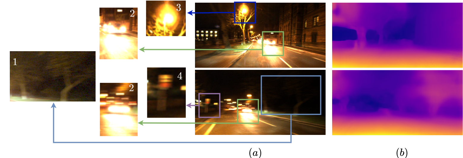
Figure 1: (a) The challenges posed by night-time images: (1) low visibility and noise (patch enhanced for better readability); (2) moving light sources with saturating image regions; (3) point light sources; (4) extreme motion blur. (b) Despite these adverse conditions, which violate the assumptions made by the photometric loss, our method can successfully estimate accurate depth maps.

In this paper, we address this problem by directly targeting violations of the temporal illumination consistency, static scene and noise-free assumptions on which the photometric loss relies. As shown by our day and night results in Table 1, these three together account for much of the discrepancy in performance between daytime and night-time. A lack of temporal illumination consistency caused by point light sources in the scene can cause pixels to be incorrectly matched between consecutive frames. To rectify this, we propose a novel per-pixel neural intensity transformation that learns to compensate for these light sources (see §3.2). Whilst conceptually straightforward, this approach is surprisingly effective, as our results in §4 demonstrate. Interestingly, they also show that it is able to operate well over wide (motion parallax) baselines, allowing us to leverage the better depth estimation performance that wider baselines offer. To correct for dynamic objects in the scene, as well as motion blur, we predict a per-pixel residual flow map (see §3.3) that we use to correct the reprojection correspondences induced by the estimated ego-motion and depth from the networks. This improves depth estimation performance at any time of day (see §4), but has additional theoretical benefits for night-time sequences because of the greater motion blur from which they typically suffer. Lastly, we robustify our approach against noise by incorporating Neighbour2Neighbour [17], a state-of-the-art denoising module, in our photometric loss formulation (see §3.4).

2 Related Work

Estimating depth from images has a long history in computer vision. Several methods use either stereo images [18, 19, 20], or two or more images taken from different viewing angles [21, 22, 23]. We try to solve this problem using a single monocular image, without any constraints on the scene of interest. Various methods have addressed this problem using supervised learning [6, 7, 24, 25, 26]. However, it is infeasible to have ground-truth depth maps for training on every scene, which limits the application of these methods and helps motivate unsupervised solutions to this problem.

Unsupervised Methods: Garg et al. [8] proposed a geometry-based loss function to train a network in a completely unsupervised fashion using a pair of stereo images. Monodepth [27] improved this by using differentiable image warping [28] and structural similarity-based [29] image comparison loss. SfMLearner [30] used only monocular images to jointly learn depth and ego-motion. It was further improved by combining stereo and monocular losses in [31, 32]. Later, GeoNet [33] and EPC [34] learnt per-pixel optical flow maps along with depth and ego-motion to mitigate the effect of moving objects. Some methods use GAN-based learning to train their systems [10, 35, 36]. Recently, Monodepth2 [37] extended Monodepth to the temporal domain, proposing a few architectural changes and robust loss functions to achieve state-of-the-art results. HR-Depth [38] used an effective skip connection and a convolution block to integrate spatial and semantic information. SD-SSMDE [39] introduced a two-stage training strategy to improve scale and inter-frame scale consistency in depth by utilising depth estimation from the first stage as a pseudo-label. Based on channel-wise attention, CADepth-Net [40] proposed structure perception and detail emphasis modules for capturing the context of scenes with the detail for the depth estimation. RM-Depth [41] proposed recurrent modulation units for an effective fusion of deep features with fewer parameters, and a warping-based motion field for moving objects to improve the scene rigidity, leading to enhanced depth estimation. More broadly, recent years have also seen a wide range of other advances in depth estimation, e.g. changes to the network architecture [42], the addition of extra loss functions [43], and better handling of dynamic objects [44]. However, all of these methods have been tested on standard daytime datasets, whereas our method is designed to work at night as well.

Nighttime Methods: All the methods above are trained using photometric loss as the main supervision signal, and with an assumption of temporal illumination consistency, which is not valid at night. A few methods, such as DeFeat-Net [45], ADFA [46] and [14], have explored how to estimate depth information from nighttime RGB images. DeFeat-Net [45] learns $n$-dimensional deep feature representations (assumed to be illumination-invariant) using a pixel-wise contrastive loss. The feature maps are simultaneously used along with the images for photometric loss calculation during training. ADFA [36] mimics a daytime depth estimation model by learning a new encoder that can generate ‘day-like’ features from nighttime images using a domain adaptation approach. Instead of feature translation as in [46], the authors in [14] propose a joint network for image translation and stereo image-based depth estimation. Recently, photometric losses are again used with an image enhancement module and a GAN-based depth regulariser in [47]. Liu et al. [48] divided the day and nighttime images into view-invariant and variant feature maps using separate encoders, and used the view-invariant information for depth estimation. All these methods either need two separate encoders for day and nighttime images [46, 48, 47], or need to learn an illumination-invariant feature space [45]. By contrast, our proposed method learns in a completely self-supervised fashion, without needing stereo images, ground-truth depth information or any additional feature learning.

3 Method

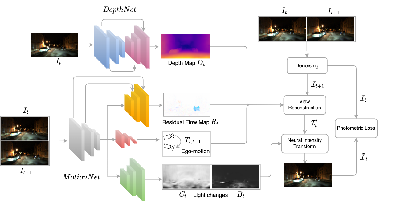
Figure 2: The architecture of our proposed method (see §3 for details).

3.1 Baseline Method

We first recap the core tenets of existing photometric loss methods, which typically use two networks, a depth network (or DepthNet) and a motion network (or MotionNet). The DepthNet takes an individual colour image as input, and is used to predict a depth image $D_{t}$ for each colour image $I_{t}$ in the input sequence. The MotionNet takes a consecutive pair of images $I_{t}$ and $I_{t+1}$ as input, and is used to output the ego-motion $T_{t,t+1}$ of the camera between them. The estimated depth and ego-motion can be used to reproject a pixel $\mathbf{u}=[u,v]^{\top}$ in frame $I_{t}$ into $I_{t+1}$, the subsequent frame in the sequence, via $\dot{V_{t}}(\mathbf{u})=KT_{t,t+1}D_{t}(\mathbf{u})K^{-1}\dot{\mathbf{u}}$, in which $\dot{\mathbf{u}}$ denotes the homogeneous form of $\mathbf{u}$, $K\in\mathbb{R}^{3\times 3}$ encodes the camera intrinsics, and $\dot{V_{t}}(\mathbf{u})\in\mathbb{R}^{3}$ denotes the homogeneous form of $V_{t}(\mathbf{u})\in\mathbb{R}^{2}$, a 2D point in the image plane of $I_{t+1}$ (which may or may not lie within the bounds of the actual image). This can be used to reconstruct an image $I^{\prime}_{t}$ by sampling from $I_{t+1}$ around the reprojected points, using bilinear interpolation [28] to achieve a smoother result. Formally,

$$\textstyle I^{\prime}_{t}(\mathbf{u})=\begin{cases}\mbox{interpolate}(I_{t+1},V_{t}(\mathbf{u}))&\mbox{if }\mathbf{u}\in M_{t}\\ \mathbf{0}&\mbox{otherwise},\end{cases}$$ (1)

in which $M_{t}=\{\mathbf{u}:\rho(V_{t}(\mathbf{u}))\in\Omega(I_{t+1})\}$ is the set of pixels whose reprojections into $I_{t+1}$, when rounded to the nearest pixel using $\rho$, fall within the image bounds $\Omega(I_{t+1})$. The reconstructed image $I^{\prime}_{t}$ can then be compared to the original image $I_{t}$ to calculate the loss values needed for training. The loss we target, namely photometric loss, has been used by many recent deep learning-based depth estimation techniques [8, 31, 30, 36]. It is normally calculated as a convex combination of pixel-wise difference and single-scale structural dissimilarity (SSIM) [29], via

$$\textstyle L_{p}^{(t)}=\frac{1}{|M_{t}|}\sum_{\mathbf{u}\in M_{t}}\left(\alpha\frac{1-\mathit{SSIM}(I_{t}(\mathbf{u}),I^{\prime}_{t}(\mathbf{u}))}{2}+(1-\alpha)\left|I_{t}(\mathbf{u})-I^{\prime}_{t}(\mathbf{u})\right|\right).$$ (2)

Most existing unsupervised methods (e.g. [30, 31, 37, 42]) use this as the backbone of their formulation. To ensure a fair comparison with current night-time state-of-the-art methods [45, 48, 47], we base our modifications in this paper on Monodepth2 [37], a commonly used baseline.

3.2 Lighting Change Compensation

The numerous point light sources that are typically turned on after dark (e.g. car headlights, lamp posts, etc.) can cause the illumination of a scene to change significantly from frame $I_{t}$ to frame $I_{t+1}$. A problematic special case occurs when a light source moves with the camera (e.g. car headlights), which can lead to large holes in the estimated depth directly in front of the ego-vehicle [45, 48]. In our approach, we compensate for the illumination changes by estimating a per-pixel transformation that, when applied to $I_{t+1}$, can mitigate the changes in lighting that have occurred since $I_{t}$. We draw some inspiration from [49, 50, 51], which use a single whole-image transformation based on two scalar values to compensate for the difference in exposure time between a pair of images, based on the observation that such a difference creates approximately uniform intensity changes over the entire image. However, in our case, the intensity changes are far from uniform over the image, owing to both the motions of the ego-vehicle and other objects in the scene, and the distances between the ego-vehicle and static point light sources. For this reason, we propose a per-pixel formulation here.

Our approach starts by passing the features produced by the last convolutional layer of the MotionNet through a lighting change decoder to estimate two per-pixel change images, $C_{t}$ and $B_{t}$ (see Figure 2). These (respectively) aim to capture the per-pixel changes in contrast (scale) and brightness (shift) that have occurred between the two input frames. As shown in Figure 4, the brightness image $B_{t}$ broadly captures the extra light added to the image by e.g. vehicle headlights, and the contrast image $C_{t}$ broadly captures the changes in ambient light due to the motion of the ego-vehicle towards or away from point light sources such as street lamps. We use these images to transform the reconstructed image $I^{\prime}_{t}$ via $\tilde{I}_{t}=C_{t}\odot I^{\prime}_{t}+B_{t}$, in which $\odot$ denotes the Hadamard product.

3.3 Motion Compensation

As seen in §3.1, the standard photometric loss makes use of correspondences between consecutive frames that have been established via reprojection, based on the ego-motion and depth estimated by the networks. Assuming that (i) the ego-motion and depth have been estimated well, (ii) the scene is static, and (iii) there is minimal motion blur, the correspondences established in this way will broadly match those that would have been established had we used the ground truth optic flow $\Phi_{t}(\cdot)$ from frame $t$ to frame $t+1$. However, if objects move with respect to the background scene, or anything visible in the image moves with respect to the ego-camera (which can cause motion blur), then the reprojection correspondences may be incorrect. To correct for these errors, we predict a residual flow map $R_{t}$, such that for each pixel $\mathbf{u}\in\Omega(I_{t})$, $R_{t}(\mathbf{u})\in\mathbb{R}^{2}$ is an estimate of $(\mathbf{u}+\Phi_{t}(\mathbf{u}))-V_{t}(\mathbf{u})$, the 2D offset from the reprojection correspondence of $\mathbf{u}$, namely $V_{t}(\mathbf{u})$, to its ground truth correspondence in frame $t+1$, namely $\mathbf{u}+\Phi_{t}(\mathbf{u})$. We can then add $R_{t}(\mathbf{u})$ to $V_{t}(\mathbf{u})$ for each pixel $\mathbf{u}$ to obtain a potentially more accurate correspondence for use in reconstructing $I^{\prime}_{t}$ via Equation 1.

Some methods [34, 33, 44] already exist that predict residual flow for daytime images. By contrast, we avoid using a separate encoder-decoder network or computationally-intensive image warping-based bilinear interpolation for supervision. Instead, we estimate residual flow using an efficient sparsity-based formulation. This involves introducing a residual flow decoder that takes the features of the final convolutional layer of the MotionNet as input and the features of previous layers in the MotionNet via skip connections, and outputs residual flow maps $\{R_{t,s}:s\in\{0,1,2,3\}\}$ at four different scales (each $R_{t,s}$ has a width and height that is $1/2^{s}$ that of $I_{t}$, and $R_{t,0}\equiv R_{t}$).

There is no direct supervision available to learn the residual flow maps. For this reason, we choose instead to encourage sparsity in the residual flow estimates, so that the estimated depth and ego-motion can explain the majority of the scene, and the left-over can be explained by the residual flow maps. To achieve this, we adopt the sparsity loss from [44], i.e.

$$\textstyle L_{r}^{(t)}=\sum_{s=0}^{3}\langle|R_{t,s}|\rangle/2^{s}\sum_{\mathbf{u}\in\Omega(I_{t,s})}\sqrt{1+|R_{t,s}(\mathbf{u})|/\langle|R_{t,s}|\rangle},$$ (3)

in which $I_{t,s}$ is a downsampled version of $I_{t}$ at scale $s$, and $\langle|R_{t,s}|\rangle$ is the spatial average of the absolute residual flow map $|R_{t,s}|$. By contrast with [44], here we introduce a normalising factor of $1/2^{s}$ at each scale, since the original loss was for scene flow, where the flow magnitude is independent of the resolution of the flow maps, which is not the case for the 2D residual flow we consider.

3.4 Image Denoising

Image noise is yet another key factor that affects the performance of the photometric loss. In practice, it is independent of the respective image, and is mainly caused by a low SNR in the darker regions of the image. Handling this noise is of crucial importance, as photometric loss is the only training signal, and supervises all of the modules we have mentioned thus far. To remove the noise from the images, we chose to use Neighbour2Neighbour [17], a state-of-the-art unsupervised denoising model trained on ImageNet with zero-mean Gaussian noise. The standard deviation values were varied from $5$ to $50$ during training. This model can either be used to denoise all images input to the network at both training time and test time, or it can be used solely at training time to denoise the images for the purpose of calculating the loss. In practice, we chose the latter approach, as denoising at test time has two major disadvantages: (i) it can significantly add to the computational burden at runtime, slowing down the depth estimation; and (ii) any errors in the denoising process can lead to downstream errors in the depth maps, even though the depth estimation model itself might have been trained well. By contrast, restricting denoising to training time has the advantage of allowing us to make the depth and motion networks robust to noise by training them on the original images.

3.5 Full Pipeline

We can now formulate our full pipeline as follows:

$$\textstyle D_{t} =\textstyle\mathcal{D}(I_{t}),\;f_{n}=\mathcal{ME}_{1:n}([I_{t},I_{t+1}])$$ (4)

$$\textstyle T_{t,t+1} =\textstyle\mathcal{MD}(f_{N}),\;R_{t}=\mathcal{RFD}(\{f_{n}:1\leq n\leq N\}),\;(C_{t},B_{t})=\mathcal{LCD}(f_{N})$$

$$\textstyle\mathcal{I}_{t} =\textstyle\mathcal{DN}(I_{t}),\;\mathcal{I}_{t+1}=\mathcal{DN}(I_{t+1})$$

$$\textstyle\mathcal{I}^{\prime}_{t} =\textstyle\mbox{reconstruct}(\mathcal{I}_{t+1},V_{t}+R_{t})$$

$$\textstyle\mathcal{\tilde{I}}_{t} =\textstyle C_{t}\odot\mathcal{I}^{\prime}_{t}+B_{t}$$

$$\textstyle L_{p}^{(t)} =\textstyle\frac{1}{|M_{t}|}\sum_{\mathbf{u}\in M_{t}}\left(\alpha\frac{1-\mathit{SSIM}(\mathcal{I}_{t}(\mathbf{u}),\mathcal{\tilde{I}}_{t}(\mathbf{u}))}{2}+(1-\alpha)\left|\mathcal{I}_{t}(\mathbf{u})-\mathcal{\tilde{I}}_{t}(\mathbf{u})\right|\right)$$

The inputs to our system are a consecutive pair of images $I_{t}$ and $I_{t+1}$, whilst $\mathcal{D}$ denotes the DepthNet, $\mathcal{ME}_{1:n}$ denotes the first $n$ layers of the $N$-layer MotionNet encoder, $\mathcal{MD}$ denotes the MotionNet decoder, $\mathcal{RFD}$ denotes the residual flow decoder, $\mathcal{LCD}$ denotes the lighting change decoder, and $\mathcal{DN}$ denotes the denoiser [17]. The reconstruct function reconstructs $\mathcal{I}^{\prime}_{t}$ as per Equation 1.

3.6 Making the Pipeline Bidirectional

Monodepth2 [37] calculates its photometric loss not only in the forwards direction, from $I_{t}$ to $I_{t+1}$, but also in the backwards direction, from $I_{t}$ to $I_{t-1}$, before combining the losses. This allows us to use the idea of minimum reprojection error to account for occluded pixels, and so we do the same. We also adopt the auto-masking losses $L_{a}^{(t)}$ from Monodepth2 [37], as even though our method can cope with moving objects, it is very difficult to use parallax to disentangle the motion of objects that are moving in the same direction and at the same speed as the ego-vehicle. We further include the commonly used edge-aware gradient smoothing loss $L_{g}^{(t)}$ [37] to maintain spatial smoothness over the estimated depth maps. Our final loss $L^{(t)}$ then becomes the weighted sum

$$\textstyle L^{(t)}=\min\left(L_{p-}^{(t)},L_{p+}^{(t)},L_{a-}^{(t)},L_{a+}^{(t)}\right)+\lambda_{r}\left(L_{r-}^{(t)}+L_{r+}^{(t)}\right)+\lambda_{g}L_{g}^{(t)},$$ (5)

in which $+$/$-$ denote the forward/backward versions of the losses, and $\lambda_{r},\lambda_{g}\in\mathbb{R}$ are the weights.

4 Experiments

In §4.1, we compare our depth estimation performance to a number of state-of-the-art approaches in a variety of different daytime and/or night-time contexts. In §4.2, we present a study on the effect of parallax to help explain the importance of our neural intensity transformation module. Finally, in §4.3, we perform an ablation study to analyse the contributions made by the three individual components of our approach. Further experiments can be found in the supplementary material.

4.1 Depth Evaluation

We compare with $4$ state-of-the-art unsupervised monocular methods: Monodepth2 [37], DeFeat-Net [45], ADDS-Depth-Night [48] and RNW [47] (see Figure 3 and Table 1). We tested our model with 3 different data variations: day only ($d$), night only ($n$), and a mix of day and night ($d\&n$). Monodepth2 [37] can be trained with all 3 configurations, although it has already been outperformed by DeFeat-Net [45] in the $d\&n$ setting. For the $d$ and $n$ settings, we outperform it by a significant margin in both error and accuracy (see Table 1). DeFeat-Net [45] and ADDS-Depth-Night [48] were originally trained with a $d\&n$ configuration. We evaluated the pre-trained models they released on our test split. Our method outperforms both methods by a significant margin on the nighttime sequences (see Table 1). Please note that we do not use any additional feature representation-based losses as used in DeFeat-Net [45], or paired day and night images as used in ADDS-Depth-Net [48]. RNW [47], another recent method, is also built on Monodepth2, but targets nighttime data only. As per Figure 3, our depth estimation results are sharp and better able to preserve edges than the competing methods. We also found that using a longer baseline improves depth estimation performance. However, naïvely using a wider baseline without also using our neural intensity transform can lead to a severe decrease in accuracy, particularly for nighttime images.

Test	Method	Train	Abs. Rel.	Sq. Rel.	RMSE	Log RMSE	$\delta<1.25$	$\delta<1.25^{2}$	$\delta<1.25^{3}$
Day	Monodepth2 [37]	d	0.219	4.525	7.641	0.285	0.679	0.862	0.930
	Ours	d	0.191	1.710	6.158	0.253	0.713	0.904	0.962
	DeFeat-Net [45]	d & n	0.247	2.980	7.884	0.305	0.650	0.866	0.943
	RNW [47]	d & n	0.297	2.608	7.996	0.359	0.431	0.773	0.930
	ADDS-Depth-Night [48]	d & n	0.239	2.089	6.743	0.295	0.614	0.870	0.950
	Ours	d & n	0.176	1.603	6.036	0.245	0.750	0.912	0.963
Night	Monodepth2 [37]	n	0.453	21.310	11.420	0.444	0.700	0.873	0.930
	RNW MCIE + SBM [47]	n	0.350	7.934	8.994	0.407	0.674	0.861	0.922
	Ours	n	0.186	1.656	6.288	0.248	0.728	0.919	0.969
	DeFeat-Net [45]	d & n	0.334	4.589	8.606	0.358	0.586	0.827	0.911
	ADDS-Depth-Night [48]	d & n	0.287	2.569	7.985	0.339	0.490	0.816	0.946
	RNW [47]	d & n	0.185	1.710	6.549	0.262	0.733	0.910	0.960
	Ours	d & n	0.174	1.637	6.302	0.245	0.754	0.915	0.964

Table 1: A quantitative comparison of our method. The results of Monodepth2 [37] are reported after retraining it. Those of DeFeat-Net [45] and ADDS-Depth-Night [48] are reported using the checkpoints from their public repositories. The evaluation uses a maximum depth of $50$m. Underlined methods use daytime images as main supervision or for regularisation losses.

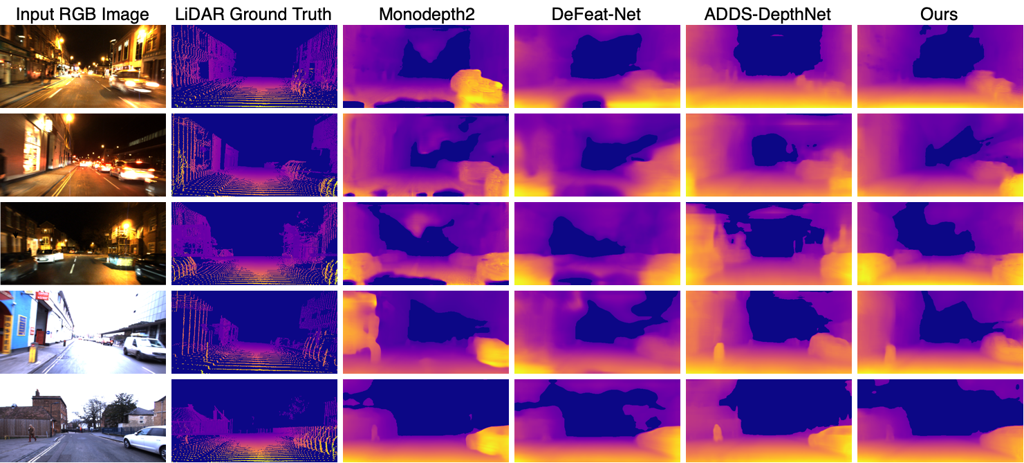
Figure 3: A qualitative comparison of our proposed method with the state of the art.

4.2 Effect of Parallax

To better understand how depth estimation performance is affected by increasing the average parallax (metric separation) between the images we use to calculate the photometric loss, we constructed a new nighttime training split by increasing the intra-triplet stride (see supplementary material) to $2$, which increased the average parallax between the images from $0.353$m to $0.706$m. Without our neural intensity transformation, the depth estimation performance significantly decreased compared to the original nighttime training split (see the difference between the RMSEs of the baseline in the top and bottom parts of Table 2). A key cause of this in night images is likely the headlights of the ego-vehicle, which can cause the pixel intensities to change drastically between frames. However, with our neural intensity transformation, the depth estimation performance was found to instead increase, which we hypothesise to be because by compensating for the lighting changes, we make it possible to exploit the stronger supervision that can be offered by a wider baseline.

4.3 Ablation Study

Lighting Change Compensation. In Figure 4(a), we show several reference images and their lighting change maps. The intensity changes are non-uniform, so we cannot use the existing correction approaches from [49, 50, 51]. We also observe that our method is able to clearly disentangle both the changes in ambient light resulting from movement towards/away from point light sources (captured by $C_{t}$) and the additional light added to the road pixels in the images by the ego-vehicle headlights (captured by $B_{t}$). Our neural intensity transform significantly reduces the RMSE error compared to the baseline (see Table 2), and is also able to fill in holes in front of the ego-vehicle (see Figure 3).

Motion Compensation. In Figure 4(b), we show several reference images and their residual flow and depth maps. In the second column, one can clearly see that our method is able to distinguish pixels on moving objects such as cars and pedestrians from static pixels. This effect can be observed for both daytime and nighttime images, showcasing the generality of our approach through a single unified training pipeline. In Table 2, it can be seen that correcting the reprojection correspondences using the residual flow map we predict leads to a significant improvement in accuracy.

Image Denoising. Denoising the images while calculating the training loss should ideally reduce the ambiguity in establishing pixel correspondences between the images, giving a robust supervision signal for training our system and thereby achieving lower error and higher accuracy. This effect can be clearly seen in the training error plot shown in Figure 4(c), where we compare our baseline+NIT model with and without denoising. The denoising results in much more accurate depth maps, improving both the RMSE and accuracy metrics as shown in Table 2.

Stride	Method	Abs. Rel.	Sq. Rel.	RMSE	Log RMSE	$\delta<1.25$	$\delta<1.25^{2}$	$\delta<1.25^{3}$
1	Baseline	0.266	5.647	6.305	0.331	0.759	0.901	0.947
	+ NIT	0.190	1.824	4.848	0.257	0.763	0.919	0.965
	+ Denoising	0.163	1.256	4.193	0.224	0.801	0.935	0.973
	Full Model	0.154	1.174	4.120	0.216	0.811	0.939	0.976
2	Baseline	0.602	63.914	14.726	0.467	0.785	0.902	0.939
	+ NIT	0.169	1.727	4.693	0.236	0.812	0.929	0.967
	Full Model	0.131	0.926	3.731	0.188	0.852	0.949	0.980

Table 2: Ablation study showing the importance of different modules in our system. The maximum depth was set to $30$m for this study. ‘Stride’ denotes intra-triplet stride (see supplementary material).

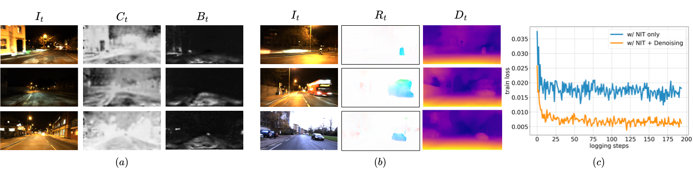
Figure 4: Visualisations of (a) estimated light changes; (b) residual flow and estimated depth; (c) the effects of denoising on the training loss over time.

5 Limitations

Our method has a number of limitations. First, as is typical of monocular methods, it is only able to estimate depth up to scale. Second, like most stereo approaches (whether variable-baseline like ours, or fixed-baseline with a rigid stereo rig), it struggles to preserve the detail of distant parts of the scene because of limited parallax. Third, it also struggles to recover structural detail from very dark image regions (e.g. see Figure 1(b)). And finally, in common with most vision-based depth estimation methods, it does not consistently perform well for transparent surfaces like glass.

6 Conclusions

In this paper, we propose a self-supervised method to learn a single model to estimate depth maps from monocular day and nighttime RGB images. By compensating for the illumination changes that can occur from one frame to the next, we enable accurate nighttime depth estimation in non-uniform lighting conditions. Moreover, by predicting per-pixel residual flow and using it to correct the reprojection correspondences induced by the estimated ego-motion and depth, we improve our method’s ability to cope with both moving objects in the scene and motion blur. Finally, by denoising the input images prior to calculating the photometric loss, we improve the loss’s ability to provide a strong supervision signal, making the entire system more robust and accurate.

Supplementary Material

Appendix A Training and Evaluation Details

A.1 Dataset Processing

We evaluated our method’s performance on both day and night sequences from the Oxford RobotCar dataset [52]. This dataset was collected over a one-year period by traversing the same route multiple times so as to include a variety of different weather and lighting conditions. We used the six sequences in the 2014-12-09-13-21-02 traversal for our daytime experiments, and the six sequences in the 2014-12-16-18-44-24 traversal for our night-time ones. We cropped the bottom 20% of each image to remove the car hood, and adjusted the camera intrinsics accordingly. We then filtered each sequence to produce a sub-sequence of keyframes such that each consecutive pair of keyframes was at least $0.5$m apart. We then constructed our training, validation and testing splits from triplets of images in the original sequence, each centred on one keyframe (at this stage with a stride of $1$). This process had the beneficial side-effect of filtering out most of the images that were captured when the ego-vehicle was stationary.

There are unfortunately no standard splits for the RobotCar dataset, and moreover the splits chosen by other methods [47, 48] overlapped geographically (see Figure 5(a)). For these reasons, we constructed our own splits by geographically dividing our triplets (constructed as above) into three daytime sets and three nighttime sets (see Figure 5(b)). The nighttime splits are comprised of $19,612$ triplets for training, $2,629$ triplets for validation and $4,559$ triplets for testing. The daytime splits are comprised of $17,790$ triplets for training, $6,693$ triplets for testing and $2,629$ triplets for validation. We used the GPS locations provided with the dataset to ensure that there was no overlap between the training and testing locations in the city. Our hope in constructing these new splits is that they will help enable fairer comparisons between methods on this dataset going forwards.

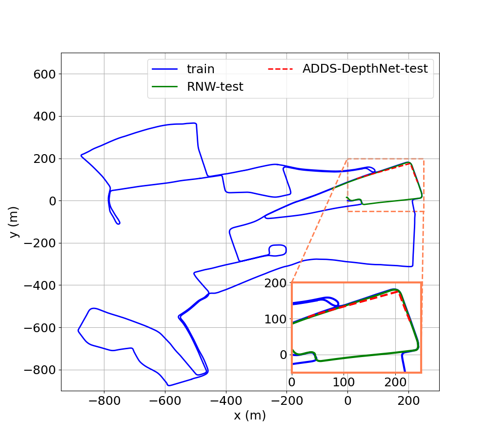
(a) Splits of RNW [47], ADDS-DepthNet [48]

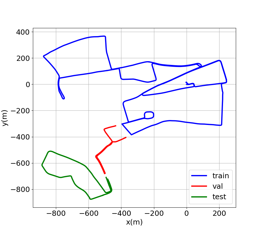
(b) Our splits

Figure 5: A geographic visualisation of the training and testing splits used by (a) RNW [47] and ADDS-DepthNet [48], and (b) our method, based on the GPS locations provided with the Oxford RobotCar dataset [52]. The splits of the methods in (a) clearly suffer from geographical overlap, whereas ours are explicitly constructed to be geographically disjoint, enabling fairer comparisons between methods on this dataset going forwards. (Best viewed in colour.)

A.2 Training

The networks were trained for $15$ epochs using PyTorch. The learning rate was set to $10^{-4}$. The loss function weights $\lambda_{r}$ and $\lambda_{g}$ (see main paper) were both set to $10^{-3}$. We used the popular Adam optimiser with $\beta_{1}=0.9$ and $\beta_{2}=0.99$ to train our network.

A.3 Evaluation

For depth evaluation, to avoid redundant computation due to the high camera frame rate, we sub-sampled the test set to have a 2m frame separation, resulting in 709 test images for nighttime and 702 images for daytime. We used the (sparse) LiDAR data provided with the dataset as ground truth for the evaluation, as no official per-pixel ground truth depth is available. As per common practice, we used a script from the Oxford RobotCar SDK to reproject LiDAR points from several nearby frames onto the current test frame to increase the number of points available for evaluation.

Scale: Like other methods trained using only monocular images, our method can only estimate depth maps up to a scale factor. When reporting results, we scale the predictions of all the methods using the median value approach suggested in [30].

Depth Truncation: Typically, a depth estimation benchmark will specify one or more maximum distance thresholds, and then, for each such threshold $\tau$, include only pixels whose ground-truth depth is $\leq\tau$ in the corresponding depth evaluation. This makes sense, since the intention is to determine the ability of a method to predict depths up to certain maximum distances.

However, for each $\tau$, most (if not all) existing unsupervised depth estimation methods also truncate their estimated depth values to $\tau$ (as opposed to e.g. counting pixels whose depth is estimated as being $>\tau$ as outliers). Unfortunately, this makes far less sense, and can have the unintended side-effect of biasing the evaluation in their favour. For example, consider a method that estimates a depth $d\gg\tau$ for a pixel $\mathbf{u}$ whose corresponding ground-truth depth is $\tau$. Without truncation, the error for this pixel will be $|d-\tau|\gg 0$, but with truncation, it will be $|\min{}(d,\tau)-\tau|=0$. In other words, this practice can lead to low errors wrongly being ascribed to mispredicted pixels, which can cause the overall error that is reported to be much lower than it otherwise would have been.

To avoid this problem, and as an alternative to explicitly counting outliers, we truncate all estimated depth values in this paper to a threshold $\tau^{\prime}\gg\tau$, thus limiting the maximum penalty for each outlier to at most $\tau^{\prime}-\tau$ (in practice, we set $\tau^{\prime}=100$m, which is much larger than $\tau=50$m, the largest maximum distance for which we report results). The difference this makes to the evaluation can be seen in Table 3.

$\tau^{\prime}$	Method	Abs. Rel.	Sq. Rel.	RMSE	Log RMSE	$\delta<1.25$	$\delta<1.25^{2}$	$\delta<1.25^{3}$
50m	RNW [47]	0.180	1.525	6.183	0.259	0.740	0.913	0.962
	Ours	0.171	1.481	6.009	0.242	0.758	0.917	0.965
100m	RNW [47]	0.185	1.710	6.549	0.262	0.733	0.910	0.960
	Ours	0.174	1.637	6.302	0.245	0.754	0.915	0.964

Table 3: The effects of truncating the depths estimated by different methods to different thresholds, for a maximum evaluation distance of $50$m, evaluated over our test set. The methods’ performance appears significantly better when the estimated depths are truncated to $50$m rather than $100$m.

Appendix B Ease-of-Deployment Comparison with State-of-the-Art Approaches

To better understand the relative deployability of our method, we compare it to three state-of-the-art approaches, namely DeFeat-Net [45], ADDS-DepthNet [48] and RNW [47]. Besides outperforming the existing models, our method also has several other advantages over them, including easier data and training requirements, as shown in Table 4.

DeFeat-Net [45] is trained with an additional feature space with pixel-wise contrastive learning, which is assumed to be illumination and weather invariant. This feature network is simultaneously learned with the depth and pose networks. We used their pre-trained model to compare against our method.

ADDS-DepthNet [48] is compared against our method using the pre-trained models released alongside their code on GitHub. The orthogonality loss proposed in their method requires corresponding daytime data. It is not possible to train this model with night-only data.

RNW [47] did not release their pre-trained models alongside their code. We retrained their model with our training data and reported the results. This method uses a GAN-based regularisation loss, through which they achieve an $\approx 93\%$ improvement over the baseline method. To achieve this, they needed to carefully train a model using daytime images, as the nighttime performance directly depends on how well the daytime model is trained.

The results reported in their paper are trained with a ResNet-50 model, whereas the model we use is ResNet-18. When we tried retraining their approach with ResNet-18, we observed a divergence of training after a few epochs. Training instability is a well-known issue that must be overcome when working with GANs, but this does highlight the relative difficulties of making even simple modifications to a GAN-based system such as RNW in comparison to our own approach. Notably, in spite of such training difficulties, RNW is the only approach that is very close to our method in terms of its error and accuracy metrics. However, unlike our method, their model can only be used for nighttime depth estimation.

Requirement	DeFeat-Net [45]	ADDS-DepthNet [48]	RNW [47]	Ours
No additional features	✗	✓	✓	✓
No daytime images	✓	✗	✗	✓
No paired day-night images	✓	✗	✓	✓
No GAN losses	✓	✓	✗	✓
Night-only training	✓	✗	✗	✓
Works for day and night	✓	✓	✗	✓

Table 4: Ease-of-deployment comparison of our method with three state-of-the-art approaches

Appendix C Ego-Motion Estimation

To evaluate the ability of our method to estimate the ego-motion of the camera, we compare the absolute trajectory error (ATE) [30, 36] it can achieve on our nighttime test sequence to the ATEs of three state-of-the-art methods, namely Monodepth2 [37], DeFeat-Net [45] and ADDS-DepthNet [48] (see Table 5). We also visualise the overall trajectory we estimate and compare it to those of other methods, as well as the ground truth (see Figure 6). Note that we estimate the ego-motion only up to scale, as our method uses monocular images during training. Moreover, the scale can drift over the course of the sequence, as there is no external constraint enforced to keep it constant.

We used the rescaling approach described in [30] for both our quantitative and qualitative pose estimation results. In both cases, our proposed method achieves results that are competitive with the state-of-the-art.

Method	$t_{ate}$ $(m)\downarrow$	$r_{ate}$ $(rad)\downarrow$
Monodepth2 [37]	0.01317 $\pm$ 0.01517	0.00036 $\pm$ 0.00040
DeFeat-Net [45]	0.03760 $\pm$ 0.01990	0.00115 $\pm$ 0.00129
ADDS-DepthNet [48]	0.01312 $\pm$ 0.01386	0.00083 $\pm$ 0.00061
Ours	0.01310 $\pm$ 0.01348	0.00041 $\pm$ 0.00039

Table 5: A quantitative comparison of our ATE errors to those of Monodepth2 [37], DeFeat-Net [45] and ADDS-DepthNet [48] on our nighttime test sequence. (The results are in the form mean $\pm$ std.)

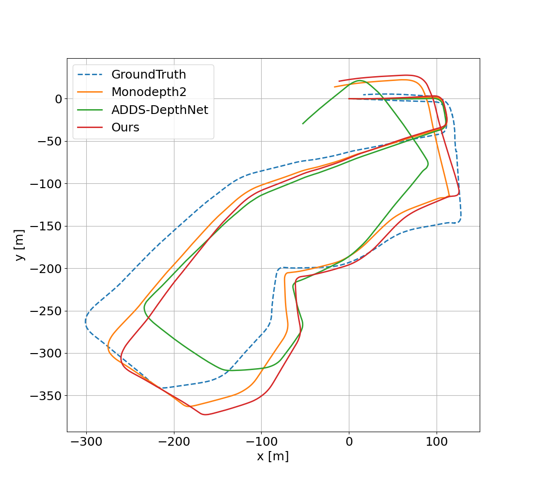
Figure 6: Comparing the trajectory estimated by our method for our nighttime test sequence to the trajectories estimated by Monodepth2 [37] and ADDS-DepthNet [48], and to the ground truth.

Appendix D Lighting Change Compensation

In this section, we aim to provide a greater understanding of the lighting change compensation technique we propose in the main paper by motivating it from first principles.

Recall that at frame $t$, our approach first predicts two per-pixel change images, $C_{t}$ and $B_{t}$, that aim to capture the per-pixel changes in contrast (scale) and brightness (shift) that occur between frame $t$ and frame $t+1$. It then uses these change images to transform the reconstructed image $I^{\prime}_{t}$ via $\tilde{I}_{t}=C_{t}\odot I^{\prime}_{t}+B_{t}$ before it is compared with image $I_{t}$.

A natural question to ask about this is: ‘why is this linear transformation an appropriate model of the lighting changes between frames $t$ and $t+1$?’ In this section, we will attempt to provide an answer.

D.1 Theoretical Background

Image Formation: Recall the basic Phong illumination model from Computer Graphics, which calculates the brightness at a 3D point $\mathbf{p}$ in world space when viewed from a direction $-\mathbf{\hat{V}}(\mathbf{p})$:

$$B(\mathbf{p})=B_{a}k_{a}+k_{d}\sum_{l\in\mathit{lights}}B_{l}\left((\mathbf{\hat{N}}(\mathbf{p})\cdot\mathbf{\hat{L}}_{l}(\mathbf{p}))+k_{s}(\mathbf{\hat{R}}_{l}(\mathbf{p})\cdot\mathbf{\hat{V}}(\mathbf{p}))^{k_{n}}\right).$$ (6)

In this, as usual, $B_{a}$ denotes the ambient illumination, $B_{l}$ denotes the brightness of light $l$, $\{k_{a},k_{d},k_{s}\}$ denote the {ambient,diffuse,specular} reflection coefficients and $k_{n}$ the specular exponent associated with the surface material, $\mathbf{\hat{N}}(\mathbf{p})$ denotes the unit normal to the surface at $\mathbf{p}$, $\mathbf{\hat{L}}_{l}(\mathbf{p})$ denotes a unit vector from $\mathbf{p}$ towards $\mathbf{p}_{l}$, the position of light $l$, $\mathbf{\hat{R}}_{l}(\mathbf{p})$ denotes the result of reflecting $\mathbf{\hat{L}}_{l}(\mathbf{p})$ across $\mathbf{N}(\mathbf{p})$, and $\mathbf{\hat{V}}(\mathbf{p})$ denotes a unit vector from $\mathbf{p}$ towards the viewer.

The image formation process can then be modelled as

$$I(\mathbf{u})=f(e\mathcal{V}(\mathbf{u})B(\mathbf{p})),$$ (7)

in which $\mathbf{u}$ is the pixel corresponding to $\mathbf{p}$ on the image plane, $f$ denotes the camera response function, $e$ denotes the exposure time, and $\mathcal{V}$ denotes the Vignetting function. This is commonly simplified (e.g. [49, 51]) by assuming that $f$ is the identity function and that there is no Vignetting effect, in which case the model simplifies to

$$I(\mathbf{u})=eB(\mathbf{p}).$$ (8)

Further Simplification: For our purposes here, we will simplify this model still further by assuming that the only illumination in the scene is diffuse, which allows us to approximate $B(\mathbf{p})$ as

$$B(\mathbf{p})\approx k_{d}\sum_{l\in\mathit{lights}}B_{l}(\mathbf{\hat{N}}(\mathbf{p})\cdot\mathbf{\hat{L}}_{l}(\mathbf{p})).$$ (9)

Whilst this assumption is not really true in practice (though the ambient illumination at night is likely to be negligible), it will significantly simplify our derivation in what follows.

Lighting Change Model: To model the change in lighting between frames $t$ and $t+1$ for a 3D world-space point $\mathbf{p}$ that is imaged at pixels $\mathbf{u}$ in $I_{t}$ and $\mathbf{u}^{\prime}$ in $I_{t+1}$, we can first approximate $I_{t}(\mathbf{u})$ and $I_{t+1}(\mathbf{u^{\prime}})$ using our image formation model:

$$I_{t}(\mathbf{u}) \approx e^{(t)}\;k_{d}\sum_{l\in\mathit{lights}}B_{l}^{(t)}(\mathbf{\hat{N}}(\mathbf{p})\cdot\mathbf{\hat{L}}_{l}^{(t)}(\mathbf{p}))$$ (10)

$$I_{t+1}(\mathbf{u^{\prime}}) \approx e^{(t+1)}\;k_{d}\sum_{l\in\mathit{lights}}B_{l}^{(t+1)}(\mathbf{\hat{N}}(\mathbf{p})\cdot\mathbf{\hat{L}}_{l}^{(t+1)}(\mathbf{p})).$$

In this, $e^{(t)}$ denotes the exposure time at frame $t$, $B_{l}^{(t)}$ denotes the brightness of light $l$ at frame $t$ and $\mathbf{\hat{L}}_{l}^{(t)}(\mathbf{p})$ denotes a unit vector from $\mathbf{p}$ towards $\mathbf{p}_{l}^{(t)}$, the position of light $l$ at frame $t$. Note that both the brightness and the position of each light in the scene are now assumed to potentially vary with time (e.g. a car headlight will move with the car).

We next observe that both $I_{t}$ and $I_{t+1}$ are actually 3-channel RGB images, not single-channel intensity images as in the simplest version of the Phong illumination model. In Computer Graphics, this is commonly handled by assigning a 3-channel RGB colour to each light, thus making each $B_{l}^{(t)}$ a 3-channel vector. However, it is more physically correct to think of the diffuse reflection coefficient $k_{d}$ as a 3-channel vector that captures the extent to which different components of white light get reflected/absorbed by the surface material. Moreover, it will turn out to be possible to eliminate $k_{d}$ in this case, and so for our purposes here, we will take this latter view.

To eliminate $k_{d}$, it suffices to divide $I_{t}(\mathbf{u})$ by $I_{t+1}(\mathbf{u^{\prime}})$ via

$$I_{t}(\mathbf{u})\oslash I_{t+1}(\mathbf{u})\approx\frac{e^{(t)}\sum_{l\in\mathit{lights}}B_{l}^{(t)}(\mathbf{\hat{N}}(\mathbf{p})\cdot\mathbf{\hat{L}}_{l}^{(t)}(\mathbf{p}))}{e^{(t+1)}\sum_{l\in\mathit{lights}}B_{l}^{(t+1)}(\mathbf{\hat{N}}(\mathbf{p})\cdot\mathbf{\hat{L}}_{l}^{(t+1)}(\mathbf{p}))}\mathbbm{1}=C_{t}^{\star}(\mathbf{u})\mathbbm{1},$$ (11)

in which $\oslash$ denotes Hadamard division and $\mathbbm{1}=(1,1,1)^{\top}\in\mathbb{R}^{3}$. This yields a scalar, $C_{t}^{\star}(\mathbf{u})$, that can clearly be multiplied by $I_{t+1}(\mathbf{u^{\prime}})$ to approximate $I_{t}(\mathbf{u})$ via $C_{t}^{\star}(\mathbf{u})I_{t+1}(\mathbf{u^{\prime}})\approx I_{t}(\mathbf{u})$. Interestingly, since $I^{\prime}_{t}(\mathbf{u})\approx I_{t+1}(\mathbf{u^{\prime}})$ as per the definition in the main paper, this means that $C_{t}^{\star}(\mathbf{u})I^{\prime}_{t}(\mathbf{u})\approx I_{t}(\mathbf{u})$, which we can also write as

$$I_{t}\approx C_{t}^{\star}\odot I^{\prime}_{t}.$$ (12)

This corresponds to a single-channel lighting change model in which we will aim to compensate for the lighting changes in $I^{\prime}_{t}$ by simply multiplying the value of each pixel in $I^{\prime}_{t}$ by its corresponding scaling factor.

D.2 Scale-only Model

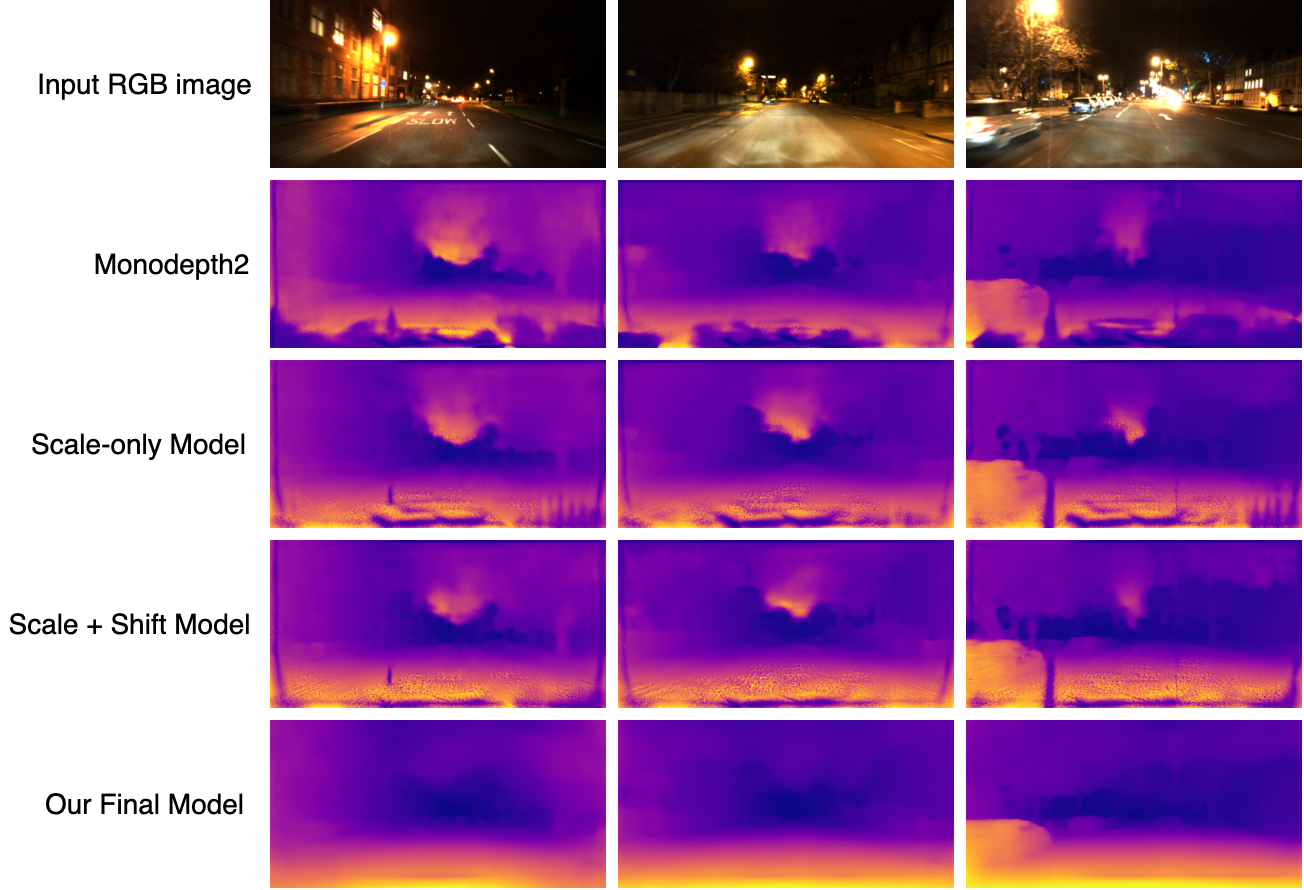
Figure 7: A qualitative comparison showing the differences in depth estimation performance between Monodepth2 [37], our scale-only lighting change model (see §D.2) and our scale + shift lighting change model (see §D.3). Our final model (which additionally includes the motion compensation and denoising components) achieves the best overall performance.

Based on the theoretical formulation in the previous sub-section, it makes sense to try to predict a single per-pixel change image $C_{t}$ for each frame $t$ (using a single-channel variant of the lighting change decoder described in the main paper) that can take the place of $C_{t}^{\star}$ in Equation 12 and be used to multiply $I^{\prime}_{t}$ to compensate for lighting changes. The effects of applying such a scale-only lighting change compensation technique to Monodepth2 [37] can be seen in Figure 7, in which it can be clearly seen that e.g. the sizes of the holes directly in front of the car have been significantly reduced. Noticeably, however, our scale-only model still struggles to cope with the strong intensity discontinuities caused by the car headlights in the close-range image region.

D.3 Scale + Shift Model

Since the scale-only model is a purely linear intensity transform, an additive term in the form of a shift channel $B_{t}$ enables an affine transformation, which provides an additional degree of freedom to the network for learning a suitable intensity transformation per pixel. As shown in Figure 7, this results in significant improvements in the estimated depth for the affected areas. We observed that our affine (scale+shift) model specifically improved depth estimation for pixels close to the camera that represent textureless road patches illuminated non-uniformly by the ego-vehicle’s headlights. We hypothesise that given the specific nature of this image region, the affine model benefits from additional learnable parameters.

Acknowledgments

This work was supported by Amazon Web Services via the Oxford-Singapore Human-Machine Collaboration Programme.

References

- Yurtsever et al. [2020] E. Yurtsever, J. Lambert, A. Carballo, and K. Takeda. A Survey of Autonomous Driving: Common Practices and Emerging Technologies. IEEE Access, 8:58443–58469, 2020.
- Sanchez et al. [2018] J. Sanchez, J.-A. Corrales, B.-C. Bouzgarrou, and Y. Mezouar. Robotic manipulation and sensing of deformable objects in domestic and industrial applications: a survey. IJRR, 37(7):688–716, 2018.
- Livingston et al. [2009] M. A. Livingston, Z. Ai, J. E. Swan, and H. S. Smallman. Indoor vs. Outdoor Depth Perception for Mobile Augmented Reality. In IEEE Virtual Reality Conference, pages 55–62, 2009.
- Newcombe et al. [2011] R. A. Newcombe, S. J. Lovegrove, and A. J. Davison. DTAM: Dense Tracking and Mapping in Real-Time. In ICCV, pages 2320–2327, 2011.
- Wang and Shen [2018] K. Wang and S. Shen. MVDepthNet: Real-time Multiview Depth Estimation Neural Network. In 3DV, pages 248–257, 2018.
- Eigen et al. [2014] D. Eigen, C. Puhrsch, and R. Fergus. Depth Map Prediction from a Single Image using a Multi-Scale Deep Network. In NeurIPS, pages 2366–2374, 2014.
- Liu et al. [2015] F. Liu, C. Shen, and G. Lin. Deep Convolutional Neural Fields for Depth Estimation from a Single Image. In CVPR, pages 5162–5170, 2015.
- Garg et al. [2016] R. Garg, V. K. BG, G. Carneiro, and I. Reid. Unsupervised CNN for Single View Depth Estimation: Geometry to the Rescue. In ECCV, pages 740–756, 2016.
- Zhan et al. [2018] H. Zhan, R. Garg, C. S. Weerasekera, K. Li, H. Agarwal, and I. Reid. Unsupervised Learning of Monocular Depth Estimation and Visual Odometry with Deep Feature Reconstruction. In CVPR, pages 340–349, 2018.
- Almalioglu et al. [2019] Y. Almalioglu, M. R. U. Saputra, P. P. B. de Gusmão, A. Markham, and N. Trigoni. GANVO: Unsupervised Deep Monocular Visual Odometry and Depth Estimation with Generative Adversarial Networks. In ICRA, pages 5474–5480, 2019.
- Kerl et al. [2013a] C. Kerl, J. Sturm, and D. Cremers. Dense Visual SLAM for RGB-D Cameras. In IROS, pages 2100–2106, 2013a.
- Kerl et al. [2013b] C. Kerl, J. Sturm, and D. Cremers. Robust Odometry Estimation for RGB-D Cameras. In ICRA, pages 3748–3754, 2013b.
- Comport et al. [2007] A. I. Comport, E. Malis, and P. Rives. Accurate Quadrifocal Tracking for Robust 3D Visual Odometry. In ICRA, pages 40–45, 2007.
- Sharma et al. [2020] A. Sharma, L.-F. Cheong, L. Heng, and R. T. Tan. Nighttime Stereo Depth Estimation using Joint Translation-Stereo Learning: Light Effects and Uninformative Regions. In 3DV, pages 23–31, 2020.
- Portz et al. [2012] T. Portz, L. Zhang, and H. Jiang. Optical Flow in the Presence of Spatially-Varying Motion Blur. In CVPR, pages 1752–1759, 2012.
- Rav-Acha and Peleg [2000] A. Rav-Acha and S. Peleg. Restoration of Multiple Images with Motion Blur in Different Directions. In Proceedings of the Fifth IEEE Workshop on Applications of Computer Vision, pages 22–28, 2000.
- Huang et al. [2021] T. Huang, S. Li, X. Jia, H. Lu, and J. Liu. Neighbor2Neighbor: Self-Supervised Denoising from Single Noisy Images. In CVPR, pages 14781–14790, 2021.
- Scharstein and Szeliski [2002] D. Scharstein and R. Szeliski. A Taxonomy and Evaluation of Dense Two-Frame Stereo Correspondence Algorithms. IJCV, 47(1-3):7–42, 2002.
- Scharstein and Pal [2007] D. Scharstein and C. Pal. Learning Conditional Random Fields for Stereo. In CVPR, pages 1–8, 2007.
- Zou and Li [2010] L. Zou and Y. Li. A Method of Stereo Vision Matching Based on OpenCV. In International Conference on Audio, Language and Image Processing, pages 185–190, 2010.
- Schönberger and Frahm [2016] J. L. Schönberger and J.-M. Frahm. Structure-from-Motion Revisited. In CVPR, pages 4104–4113, 2016.
- Dai et al. [2013] Y. Dai, H. Li, and M. He. Projective Multiview Structure and Motion from Element-Wise Factorization. TPAMI, 35(9):2238–2251, 2013.
- Yu and Gallup [2014] F. Yu and D. Gallup. 3D Reconstruction from Accidental Motion. In CVPR, pages 3986–3993, 2014.
- Ladický et al. [2014] L. Ladický, J. Shi, and M. Pollefeys. Pulling Things out of Perspective. In CVPR, pages 89–96, 2014.
- dos Santos Rosa et al. [2019] N. dos Santos Rosa, V. Guizilini, and V. Grassi Jr. Sparse-to-Continuous: Enhancing Monocular Depth Estimation using Occupancy Maps. In International Conference on Advanced Robotics, pages 793–800, 2019.
- Fu et al. [2018] H. Fu, M. Gong, C. Wang, K. Batmanghelich, and D. Tao. Deep Ordinal Regression Network for Monocular Depth Estimation. In CVPR, pages 2002–2011, 2018.
- Godard et al. [2017] C. Godard, O. Mac Aodha, and G. J. Brostow. Unsupervised Monocular Depth Estimation with Left-Right Consistency. In CVPR, pages 6602–6611, 2017.
- Jaderberg et al. [2015] M. Jaderberg, K. Simonyan, A. Zisserman, and K. Kavukcuoglu. Spatial Transformer Networks. In NeurIPS, pages 2017–2025, 2015.
- Wang et al. [2004] Z. Wang, A. C. Bovik, H. R. Sheikh, and E. P. Simoncelli. Image Quality Assessment: From Error Visibility to Structural Similarity. TIP, 13(4):600–612, 2004.
- Zhou et al. [2017] T. Zhou, M. Brown, N. Snavely, and D. G. Lowe. Unsupervised Learning of Depth and Ego-Motion from Video. In CVPR, pages 1851–1860, 2017.
- Vankadari et al. [2018] M. B. Vankadari, K. Das, A. Majumdar, and S. Kumar. UnDEMoN: Unsupervised Deep Network for Depth and Ego-Motion Estimation. In IROS, pages 1082–1088, 2018.
- Li et al. [2018] R. Li, S. Wang, Z. Long, and D. Gu. UnDeepVO: Monocular Visual Odometry through Unsupervised Deep Learning. In ICRA, pages 7286–7291, 2018.
- Yin and Shi [2018] Z. Yin and J. Shi. GeoNet: Unsupervised Learning of Dense Depth, Optical Flow and Camera Pose. In CVPR, pages 1983–1992, 2018.
- Luo et al. [2020] C. Luo, Z. Yang, P. Wang, Y. Wang, W. Xu, R. Nevatia, and A. Yuille. Every Pixel Counts++: Joint Learning of Geometry and Motion with 3D Holistic Understanding. TPAMI, 42(10):2624–2641, 2020.
- Aleotti et al. [2018] F. Aleotti, F. Tosi, M. Poggi, and S. Mattoccia. Generative Adversarial Networks for unsupervised monocular depth prediction. In ECCV-W, 2018.
- Vankadari et al. [2019] M. Vankadari, S. Kumar, A. Majumder, and K. Das. Unsupervised Learning of Monocular Depth and Ego-Motion using Conditional PatchGANs. In IJCAI, pages 5677–5684, 2019.
- Godard et al. [2019] C. Godard, O. Mac Aodha, M. Firman, and G. Brostow. Digging Into Self-Supervised Monocular Depth Estimation. In ICCV, pages 3828–3838, 2019.
- Lyu et al. [2021] X. Lyu, L. Liu, M. Wang, X. Kong, L. Liu, Y. Liu, X. Chen, and Y. Yuan. HR-Depth: High Resolution Self-Supervised Monocular Depth Estimation. In AAAI, pages 2294–2301, 2021.
- Petrovai and Nedevschi [2022] A. Petrovai and S. Nedevschi. Exploiting Pseudo Labels in a Self-Supervised Learning Framework for Improved Monocular Depth Estimation. In CVPR, pages 1578–1588, 2022.
- Yan et al. [2021] J. Yan, H. Zhao, P. Bu, and Y. Jin. Channel-Wise Attention-Based Network for Self-Supervised Monocular Depth Estimation. In 3DV, pages 464–473, 2021.
- Hui [2022] T.-W. Hui. RM-Depth: Unsupervised Learning of Recurrent Monocular Depth in Dynamic Scenes. In CVPR, pages 1675–1684, 2022.
- Guizilini et al. [2020] V. Guizilini, R. Ambru\cbs, S. Pillai, A. Raventos, and A. Gaidon. 3D Packing for Self-Supervised Monocular Depth Estimation. In CVPR, pages 2485–2494, 2020.
- Shu et al. [2020] C. Shu, K. Yu, Z. Duan, and K. Yang. Feature-metric Loss for Self-supervised Learning of Depth and Egomotion. In ECCV, pages 572–588, 2020.
- Li et al. [2021] H. Li, A. Gordon, H. Zhao, V. Casser, and A. Angelova. Unsupervised Monocular Depth Learning in Dynamic Scenes. PMLR, 155:1908–1917, 2021.
- Spencer et al. [2020] J. Spencer, R. Bowden, and S. Hadfield. DeFeat-Net: General Monocular Depth via Simultaneous Unsupervised Representation Learning. In CVPR, pages 14402–14413, 2020.
- Vankadari et al. [2020] M. Vankadari, S. Garg, A. Majumder, S. Kumar, and A. Behera. Unsupervised Monocular Depth Estimation for Night-time Images using Adversarial Domain Feature Adaptation. In ECCV, pages 443–459, 2020.
- Wang* et al. [2021] K. Wang*, Z. Zhang*, Z. Yan, X. Li, B. Xu, J. Li, and J. Yang. Regularizing Nighttime Weirdness: Efficient Self-supervised Monocular Depth Estimation in the Dark. In ICCV, pages 16055–16064, 2021.
- Liu et al. [2021] L. Liu, X. Song, M. Wang, Y. Liu, and L. Zhang. Self-supervised Monocular Depth Estimation for All Day Images using Domain Separation. In ICCV, pages 12737–12746, 2021.
- Jin et al. [2001] H. Jin, P. Favaro, and S. Soatto. Real-Time Feature Tracking and Outlier Rejection with Changes in Illumination. In ICCV, volume 1, pages 684–689, 2001.
- Baker and Matthews [2004] S. Baker and I. Matthews. Lucas-Kanade 20 Years On: A Unifying Framework. IJCV, 56(3):221–255, 2004.
- Yang et al. [2020] N. Yang, L. v. Stumberg, R. Wang, and D. Cremers. D3VO: Deep Depth, Deep Pose and Deep Uncertainty for Monocular Visual Odometry. In CVPR, pages 1281–1292, 2020.
- Maddern et al. [2017] W. Maddern, G. Pascoe, C. Linegar, and P. Newman. 1 year, 1000 km: The Oxford RobotCar Dataset. IJRR, 36(1):3–15, 2017.