Sampling spatial  Structures in geostatistical framework

Abstract

Extreme values geostatistics make it possible to model the asymptotic behaviors of random phenomena which depends on space or time parameters. In this paper, we propose new models of the extremal coefficient within a spatial stationary fields underlied by multivariate copulas. Some models of extensions of the extremogram and the cross-extremogram are constructed in a spatial framework. Moreover, both these two geostatistcal tools are modeled using the extremal variogram which characterizes the asymptotic stochastic behavior of the phenomena.

Keywords Extremal index, extremogram, variogram, copulas, stationary process, extreme values distributions

2010 MSC: 60G70, 62H11, 60G10.

1 Introduction

Geostatistics provide many tools for statistical analysis of spatial or spatio temporal datasets. This branch of statistics was developed originally in the years $1930$ by a pionering work of George Matheron [22] to predict the probability distributions of more grades for mining operations. Since, it became a subdomain of statistics based on the notion of random fields including petroleum geology, hydrogeology, geochemistry, geometallurgy, geography, forestry, environmental control, landscape ecology, soil science and agriculture.

In spatial statistical analysis, the variograms and the covariance functions are technical tools used in describing how the spatial continuity changes with a given separating distance between two pair of stations. So, the classical variogram provides a framework for modelling and predicting the variability of a given the stochastic spatial process.

The family of copulas provides a natural way to construct multivariate distribtutions whose marginals are uniform and not necessarily exchangeable. Let $X=\left(X_{1},...,X_{n}\right)$ be a random vector with multivariate continuous distribution function (c.d.f.) H and c.d.f marginal $H_{1},...,H_{n}.$ The copula of X (of the c.d.f. H respectively) is the multivariate c.d.f. C of the random vector $U=\left[H_{1}(x_{1}),\dots,H_{n}(x_{n})\right]$. Due to the continuity of $\left\{H_{i},1\leq i\leq n\right\},$ each component of U is standard uniformly distributed, i.e., $U_{i}\sim U(0,1)$ for $i=1,\dots,n.$

Particularly, every n-copula must satisfy the n-increasing property [14]. That means that, for any rectangle $B=\left[a,b\right]^{n}\subseteq\mathbb{R}^{n},$ the B-volume $C_{B}$ of C is positive, that is,

$$C_{B}=\int_{B}dC\left(u\right)=\sum_{i_{1}=1}^{2}\dots\sum_{i_{n}=1}^{2}\left(-1\right)^{i_{1}+\dots+i_{n}}C\left(u_{1i_{1}},\dots,u_{1i_{n}}\right)\geq 0.$$ (1)

In multivariate copulas analysis following canonical parameterization of H (see [4]) allows the use of copulas in stochastic analysis under the so called Sklar theorem $\left[9\right]$ or Nelsen $\left[12\right]$

$$C(u_{1},...,u_{n})=H[H_{1}^{-1}(u_{1}),...,H_{n}^{-1}(u_{n})]$$.

(2)

H^-1 being the generalized inverse such as $H^{-1}\left(x\right)=\inf\left\{t\in\left[0,1\right],F\left(t\right)\leq x\right\}$.

While modeling the main geostatistical tools Ouoba et al. [13]  have provided the copula-based variogram, correlogram and madogam and they pointed out that these tools do not take into account the extreme data observed in the different observation sites. However, the copula function makes it possible to model the extreme data and make it possible to detect any nonlinear link between different observation sites. It is therefore necessary to express the variogram and the covariogram according to the copula in order to be able to model the spatial structuring even if our giving includes extremes and to be able to detect the presence of some nonlinear dependence.
The variogram

$$\vartheta(s_{i},s_{j})=Var(Z(s_{i}))+Var(Z(s_{j}))-2\hat{c}(s_{i},s_{j}),$$

the covariogram $\hat{c}(s_{i},s_{j})$ and the copula function are linked by the relation:

$$\vartheta(s_{i},s_{j})=\sigma_{Z}^{2}(s_{i})+\sigma_{Z}^{2}(s_{j})-2\int_{0}^{1}\int_{0}^{1}F_{Z}^{-1}(u)F_{Z}^{-1}(v)c(u,v)dudv-2m_{i}m_{j}$$

$$\hat{c}(s_{i},s_{j})=\int_{0}^{1}\int_{0}^{1}F_{Z}^{-1}(u)F_{Z}^{-1}(v)c(u,v)dudv-m_{i}m_{j}$$

where $m_{i}$ and $m_{j}$ the respective averages of $Z(s_{i})$ and $Z(s_{j})$; $c(u,v)$ the copula density function attached to $Z(s_{i})$ and $Z(s_{j})$.

The major contribution of this article is to provide tools to model the dependence of extremes in the mining context. In section 2 we develop the tools needed to achieve our goals. Our main results are given in section 3, where we propose new models of the extremal coefficient in a spatial stationary field using multivariate copulas and the extensions of the extremogram and the crossed extremogram in a spatial framework using the extremal variogram which characterizes the asymptotic stochastic behavior of phenomena.

2 Back Ground

In this section we collect the necessary definitions and usefull properties on extremal dependence coefficient and tail dependence. So an overview of spatial framework and copulas functions is given as well as some statements of multivariate tail dependence coefficients.

Multivariate extreme values (MEV) theory is often presented in the framework of coordinatewise maxima, so the importance of distinction diminishes. Towards a multivariate analogue of Fisher-Tippett we are looking for some sort of multivariate limit distribution for conveniently normalized vectors of multivariate maxima. For an arbitrary index of set T denoting generally a space of time, a random vector $Y_{t}=\left\{Y_{j}\left(t\right);1\leq j\leq m,t\in T\right\}$ in $\mathbb{R}^{m}$ is said to be max-stable if, for all $n\in\mathbb{N},$ every $Y_{j}\left(t\right)=(Y_{j}^{(1)}\left(t\right);\ldots;Y_{j}^{(n)}\left(t\right))$ is a n-dimensionnal max-stable vector, that is, there exists suitable and time-varying non-random sequences $\left\{a_{n}\left(t\right)>0\right\}~{}~{}and~{}~{}\left\{b_{n}\left(t\right)\in\mathbb{R}^{d}\right\}~{}~{}such~{}~{}as~{}~{}$

$$\frac{1}{a_{n}(t)}\left[M_{n}(t)-b_{n}(t)\right]\stackrel{{\scriptstyle f.d.d}}{{\longrightarrow}}X(t);t\in T,$$ (3)

where $\stackrel{{\scriptstyle f.d.d}}{{\longrightarrow}}$ denotes the convergence for the finite-dimensional distributions while $M_{n}\left(t\right)=\max_{1\leq i\leq n}\left(X_{i}\left(t\right)\right);t\in T$ being the component-wise maxima of the time-variying vector $X\left(t\right)$.

Like in the non-spatial analysis, several canonical representations of max-stable processes have been suggested in spatial extreme values context.  In the same vain, Barro et al. (see [9] ) have propose the following result  allows us to characterize the general form of the one-dimensional marginal of the max-stable ST process $\left\{Y_{t}\right\}$ where $Y_{t}\left(x\right)=Y\left(x_{t}\right)$; $x_{t}\in\chi_{{}_{D}}\times T\subset R^{3}$. $\left(Y_{j}^{s}\left(t\right)\right);j\geq 0;t\in T;s\in S$ such that for each fixed couple $(t,s)$, the sequence is independent and identically distributed according to a joint cumulative function $G_{t}^{s}$. Under the assumption that this function is max-stable, every univariate margins $G_{t,i}^{s}$  lies its own domain of attraction and is expressed by on the space of interest $S_{\xi_{i},t,s}^{+}=\left\{z\in\mathbb{R};\sigma_{i,t,s}+\xi_{i,t,s}\left(y_{t,i}^{s}-\mu_{i,t,s}\right)>0;1\leq i\leq n\right\}$ by

$$G_{i}\left(y_{i}\left(s\right)\right)=\left\{\begin{tabular}[]{l}$\exp\left\{-\left[1+\xi_{i}\left(s\right)\left(\frac{y_{i}\left(s\right)-\mu_{i}\left(s\right)}{\sigma_{i}\left(s\right)}\right)\right]^{\frac{-1}{\xi_{i}\left(s_{i}\right)}}\right\}\hskip 14.22636pt$ {if }$\xi_{i}\left(s\right)\not=0$\\ \\ \\ $\exp\left\{-\exp\left\{-\left(\frac{y_{i}\left(s\right)-\mu_{i}\left(s\right)}{\sigma_{i}\left(s\right)}\right)\right\}\right\}$ \hskip 48.36958pt {if }$\xi_{i}\left(s\right)=0$\end{tabular}\right.;$$ (8)

and for all site s, the parameters $\left\{\mu_{i,t,s}\in\mathbb{R}\right\}$, $\left\{\sigma_{i,t,s}>0\right\}$ and $\left\{\xi_{i,t,s}\in\mathbb{R}\right\}$ are referred to as the location, the scale and the shape parameters respectively. Particularly, the different values of $\xi_{i}\left(s\right)\in\mathbb{R}$ allows 8 to be a spatial EV model, that is, to belong either to Frechet family, the Weibull one or Gumbel one.

In multivariate case if the one-dimensional margins of F are unit-Fréchet distributed let M be a non-empty subset of $N=\left\{1,...,n\right\}$ and $c_{{}_{M}}$ the n-dimensional vector of which the jth coordinate is one or zero according to $j\in M$ or $j\not\in M$. Then, the multivariate, $\theta_{M}$ is defined on the n-dimensional unit simplex, S${}_{n}=\left\{\left(t_{1}...,t_{n}\right)\in\left[0,1\right]^{n},\sum_{i=1}^{n}t_{i}\leq 1\right\},$ such as,

$$\theta_{M}=V(c_{{}_{M}})=\int_{S_{n}}\max_{j\in M}\left(\frac{w_{j}}{\left\|w\right\|_{1}}\right)dH\left(w_{j}\right),$$ (9)

where H is a finite non-negative measure of probability and $\left\|.\right\|_{1},$ the 1-norm, see [4], [5]. Particularly

$$P\left[F_{1}\left(x_{1}\right)\leq p,...,F_{n}\left(x_{n}\right)\leq p\right]=p^{\theta}~{}~{}for~{}~{}all~{}~{}0<p<1.$$ (10)

In spatial study, a natural way to measure dependence among spatial maxima stems from considering the distribution of the largest value that might be observed on domain of study.

Our main results are summaried by the following sections.

3 Spatial max-stability within geostatiscal framework

The extremal coefficient is the natural dependence measures for extreme value models which provides the magnitude of the asymptotic dependence of a random field at two points of the domain.

3.1 Context and definitions

The context in this study, is a mining ressource models one.

3.1.1 Problematic and variable

We consider a mining geographic area for example. By considering a subdivision, a paving of the domain. We consider a reference grade $\beta_{O}$ for the given ore. The domain is thus divided into two subdomains depending on whether the content of the locality is lower or higher than this reference.

Working hypotheses:

$\bullet$ The content depends on the locality and the depth h, that is to say $s=s\left(h\right).$

$\bullet$

The variable Y representing the content is linked to the locality $Y=Y\left(s\right)$ and therefore $Y=Y\left(s\left(h\right)\right).$ So we build a stochastic process?

In this study, let $\left\{Y_{s},s\in S\right\}$ a spatial stochastic process defined on a geographical domain $S=\left\{s_{1},\dots,s_{n}\right\}$  where $\left\{Y_{s},s\in S\right\}$ denotes the contents of a metal in a mining site.

Let n,k be naturel numbers such that $\left\{n\geq 2;~{}~{}1\leq k\leq n\right\}$ and let $N_{k}$ be a given subset of k elements of $N=\left\{1,\dots,n\right\},$ the set of the first n natural numbers.

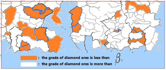
Figure 1: Domain of mining study.

Even in spatial stochastic context, three possible distributions can describe the asymptotic behavior of conveniently normalized extremal distributions at a given geographical locality s. These distributions are instead described by a class of dependence models. Specially in a spatial framework, let $D_{N}=\left\{s_{1},...,s_{N}\right\}\subset\mathbb{R}^{2}$ be the set of locations (geographical ereas, mines localities, …), sampled over a $\left[0,\frac{1}{s}\right]\times\left[0,\frac{1}{m}\right]$ rectangle $\left(m\in\mathbb{N}\right)$, where the phenomenas are observed. Let Y a variable of interest, observed at given site s and date t.

So, the relation (2.2) provides, for all $x_{t}=\left(x_{t}^{\left(1\right)};...;x_{t}^{\left(m\right)}\right)$ in $\mathbb{R}^{m}\times T$  the relation

$$C_{s(t)}(u_{1};...;u_{m})=F_{t}^{\check{s}}\left[\left(F_{t}^{\check{s}_{1}}(u_{1})\right)^{-1};...;\left(F_{t}^{\check{s}_{m}}(u_{m})\right)^{-1}\right].$$ (11)

Note that, for all $m\in\mathbb{N}$ and for all geographical locality s, the spatio-temporal unit simplex of $\mathbb{R}^{(m-1)}$ is given, under the notational by

$$\Delta_{t,m}^{\check{s}}=\left\{\lambda_{t}^{\check{s}}=\left(\lambda_{1}^{\check{s}_{1}};...;\lambda_{t}^{\check{s}_{m}}\right)\in\mathbb{R}_{+}^{m};\left\|\lambda_{t}^{\check{s}}\right\|=\sum_{i=1}^{m}\lambda_{t}^{\check{s}_{i}}=1\right\}.$$ (12)

3.1.2 Spatial max-stability

Definition 1

Let $Y=\left\{Y_{s(h)},s\in S,t\in T\right\}$ be a spatial process with parametric joint distribution $H_{t}^{\check{s}}.$ The following statements are satisfied  a sufficient condition for the process $H_{t}^{\check{s}}$ to be a ST-MEV distribution is that there exists two spatio-temporal non-random sequences $\left\{\alpha_{n}^{\check{s}}\left(t\right)>0\right\}$ and $\left\{\beta_{n}^{\check{s}}\left(t\right)\in\mathbb{R}\right\}$ such that

$$\lim_{n\uparrow\infty}P\left(\frac{M_{t}^{\check{s}}-\beta_{n}^{\check{s}}\left(t\right)}{\alpha_{n}^{\check{s}}\left(t\right)}\leq y_{t}^{\check{s}}\right)=\left(H_{1}\left(y_{t}^{\check{s}_{1}}{}\right),\dots,H_{m}\left(y_{t}^{\check{s}_{m}}{}\right)\right).$$ (13)

where $M_{t}^{\check{s}\left(i\right)}$ is univariate margins of the spatio-temporal componentwise vector of maxima.

As a corrolary of the above definition, (11) provides, for all $x_{t}=\left(x_{t}^{\left(1\right)};...;x_{t}^{\left(m\right)}\right)$ in $\mathbb{R}^{m}\times T$  the relation

$$C_{s(t)}(u_{1}^{t};...;u_{m}^{t})=H_{t}^{\check{s}}\left[\left(H_{1}^{\check{s}_{1}}(u_{1}^{t})\right);...;\left(H_{m}^{\check{s}_{m}}(u_{m}^{t})\right)\right],$$ (14)

where $u_{i}^{t}=H_{i}^{-1}\left(s_{i}(t)\right).$
Note that, for all $m\in\mathbb{N}$ and for all geographical locality s, the spatio-temporal unit simplex of $\mathbb{R}^{(m-1}$ is given, under the notational by

$$\Delta_{t,m}^{\check{s}}=\left\{\lambda_{t}^{\check{s}}=\left(\lambda_{1}^{\check{s}_{1}};...;\lambda_{t}^{\check{s}_{m}}\right)\in\mathbb{R}_{+}^{m};\left\|\lambda_{t}^{\check{s}}\right\|=\sum_{i=1}^{m}\lambda_{t}^{\check{s}_{i}}=1\right\}.$$ (15)

3.1.3 Domain Spatially discordant

In this sub-section, we consider a geographical domain D made up of several sites that we partition into two sub-domains depending on whether the sites in the domain have a mineral content higher than a reference value or not.

Definition 2

(Domain Spatially discordant)We define $N_{k}$-partition of a random vector $X=\left\{X_{1},\dots,X_{n},~{}~{}n\geq 2\right\}$ (or the partition of X in the direction of $N_{k}$) by the pairwise vector $\stackrel{{\scriptstyle\sim}}{{X}}=(\stackrel{{\scriptstyle\sim}}{{X}}_{N_{k}},\stackrel{{\scriptstyle\sim}}{{X}}_{\overline{N}_{k}})$ as:

$\bullet\stackrel{{\scriptstyle\sim}}{{X}}=(X_{N_{k},1},\dots,X_{N_{k},k})$ is the k-dimensional marginal vector of X whose component indexes are ordered in the subset $N_{k}$.

$\bullet\stackrel{{\scriptstyle\sim}}{{X}}=(X_{\overline{N}_{k},1},\dots,X_{\overline{N}_{k},n-k})$ is the $(n-k)$ dimensional marginal vector of X whose component indexes are ordered in $\overline{N}_{k}=C_{N}^{N_{k}}$, the complementary of $N_{k}$in N.

Similarly, every realisation $x=(x_{1},\dots,x_{n})$ of X can be decomposed into two parts

$$x=(\stackrel{{\scriptstyle\sim}}{{x}}_{N_{k}},\stackrel{{\scriptstyle\sim}}{{x}}_{\overline{N}_{k}})~{}~{}where~{}~{}\stackrel{{\scriptstyle\sim}}{{x}}_{N_{k}}=(x_{N_{k},1},\dots,x_{N_{k},k})~{}~{}and~{}~{}\stackrel{{\scriptstyle\sim}}{{x}}=(x_{\overline{N}_{k},1},\dots,x_{\overline{N}_{k},k})$$

are, respectively realizations of vectors $\stackrel{{\scriptstyle\sim}}{{X}}_{N_{k}}$ et $\stackrel{{\scriptstyle\sim}}{{X}}_{\overline{N}_{k}}$. If H, $H_{N_{k}}$ and $H_{\overline{N}_{k}}$ denote the distribution functions of the random vectors X, $\stackrel{{\scriptstyle\sim}}{{X}}_{N_{k}}$ and $stackrel{\sim}{X}_{\overline{N}_{k}}$, then for all realization $x=(x_{1},\dots,x_{n})$ of X we have

$$H_{N_{k}}(\stackrel{{\scriptstyle\sim}}{{x}}_{N_{k}}) = \displaystyle\lim_{\stackrel{{\scriptstyle\sim}}{{x}}_{\overline{N}_{k}}\rightarrow\stackrel{{\scriptstyle\sim}}{{x}}_{\overline{N}_{k}}^{\ast}}H(x)~{}and~{}H_{\overline{N}_{k}}(\stackrel{{\scriptstyle\sim}}{{x}}_{\overline{N}_{k}})=\displaystyle\lim_{\stackrel{{\scriptstyle\sim}}{{x}}_{N_{k}}\rightarrow\stackrel{{\scriptstyle\sim}}{{x}}_{N_{k}}^{\ast}}H(x)$$

$$~{}where~{}\stackrel{{\scriptstyle\sim}}{{x}}_{N_{k}}^{\ast} = (x_{N_{k},1}^{\ast},\dots,x_{N_{k},k}^{\ast})~{}and~{}\stackrel{{\scriptstyle\sim}}{{x}}^{\ast}=(x_{\overline{N}_{k},1}^{\ast},\dots,x_{\overline{N}_{k},k}^{\ast})$$

are the upper endpoints of the functions $H_{N_{k}}$ and $\stackrel{{\scriptstyle\sim}}{{X}}_{\overline{N}_{k}}$.

Definition 3

Given a $N_{k}-$partition $\stackrel{{\scriptstyle\sim}}{{X}}=\left\{\left(X_{N_{k}},\stackrel{{\scriptstyle\sim}}{{X}}_{\overline{N}_{k}}\right),1\leq k\leq n\right\}$ of $X=\left\{X_{1},\dots,X_{n}\right\}$ we define the upper $N_{k}-$discordance degree of X as the conditional probability given for all $x=(x_{1},\dots,x_{n})\in\mathbb{R}_{n}$ by $\delta_{N_{k}}^{+}(x)=P(\stackrel{{\scriptstyle\sim}}{{X}}_{N_{k}}>\stackrel{{\scriptstyle\sim}}{{x}}_{N_{k}}/\stackrel{{\scriptstyle\sim}}{{X}}_{\overline{N}_{k}}\leq\stackrel{{\scriptstyle\sim}}{{x}}_{\overline{N}_{k}})$. Similarly, the lower $N_{k}-$discordance degree of X is defined, for all $x=(x_{1},\dots,x_{n})\in\mathbb{R}_{n}$ by $\delta_{N_{k}}^{-}(x)=P(\stackrel{{\scriptstyle\sim}}{{X}}_{N_{k}}\leq\stackrel{{\scriptstyle\sim}}{{x}}_{N_{k}}/stackrel{\sim}{X}_{\overline{N}_{k}}>\stackrel{{\scriptstyle\sim}}{{x}}_{\overline{N}_{k}})$.

3.1.4 Spatial discordance rate

In the modeling of spatial extremes, the calculation of quantiles is very important. The following definition characterizes the probability that one of the margins $\stackrel{{\scriptstyle\sim}}{{X}}_{N_{k}}$ and $\stackrel{{\scriptstyle\sim}}{{X}}_{\overline{N}_{k}}$ exceeds $1/2$, while the values taken by the other are less than $1/2.$

Definition 4

Given the distribution H of a multivariate random vector $X=\left\{X_{1},\dots,X_{n}),n\geq 2\right\}$ with univariate margins $H_{i},1\leq i\leq n$ we define the upper $N_{k}-$median discordance degree of H by the real number denoted by $\delta_{N_{k},H}^{+}$ such as: $\delta_{N_{k},H}^{+}=\delta_{N_{k}}^{+}\left[(H_{1}^{-1}(\frac{1}{2}),\dots,H_{n}^{-1}(\frac{1}{2}))\right]$ where $H_{i}^{-1}$ is quantile function of $H_{i}.$ Similarly, the lower $N_{k}-$median discordance degree of H is defined by $\delta_{N_{k},H}^{-}=\delta_{N_{k}}^{-}\left[(H_{1}^{-1}(\frac{1}{2}),\dots,H_{n}^{-1}(\frac{1}{2}))\right]$

3.2 Spatial MDA and inferential properties

Spatial max-stable processes generalize the Multivariate Extreme Value (MEV) laws to the spatial context and hold information on the spatial dependence structure. Specifically a constructive definition is given as follows.

Definition 5

(see [9]) Let S be a spatial domain. We say that the process $\left\{Y(s),s\in\mathcal{S}\right\}$ is max-stable if all the marginal distributions are max-stable, that is to say exists for all $n$ two suites of continuous functions $\left\{\alpha_{n}(s)\right\}>0$ and $\left\{\beta_{n}(s)\right\}$ such as:

$$\lim_{n\rightarrow+\infty}\left\{\frac{\max_{i=1}^{n}X(s_{i})-\beta_{n}(s)}{\alpha_{n}(s)}\right\}=\left\{Y(s),s\in\right\},$$

with $X(s_{i})$ independent and identically distributed copies of $X$, a stochastic process representing for example a meteorological parameter. Without loss of generality and to consider only the spatial dependence of $\left\{Y(s),s\in\right\}$, it is more convenient to transform $Y$ into a simple max-stable process, ie with Frechet margins unit (ie $GEV\left(1,1,1\right)$) for all $s\in S$ via the following transformation:

$$Y_{F}(s)=\frac{-1}{\log\left\{G_{\mu(s),\sigma(s),\xi(s)}\left(Y(s)\right)\right\}}.$$

The study of extreme value theory have been extended both to spatial and multivariate contexts these last years. This section gives the relationship between the extremal coefficient via copula.

3.3 Stability spatial marginal

Theorem 6

Let G be a spatially max-stable multivariate distribution..  Then, under the condition of the max-stability of $\left\{Y\right\}$, the distributions underlying the marginal processes $\left\{Y_{t_{A}}\mathit{\ }\right\}$ and $\left\{Y_{t_{\bar{A}}}\mathit{\ }\right\}$ lies  respectively in the MDA of two parametric MEV models G_A and G${}_{\bar{A}}$. Moreover the distributions G_A and G${}_{\bar{A}}$ are marginal distributions of G.

Proof.  Let $\left\{\alpha_{n}>0\right\}$ and $\left\{\beta_{n}\in\mathbb{R}\right\}$ be the non-random  normalizing sequences of H. Then, their corresponding space and time extensions $\left\{\alpha_{n}^{\check{s}}\left(t\right)>0\right\}$ and $\left\{\beta_{n}^{\check{s}}\left(t\right)\in\mathbb{R}\right\}$ are defined on the set, $\mathbb{N}^{\ast}\times S\times T,$ such that

$$\lim_{n\uparrow\infty}P\left(\frac{M_{t}^{\check{s}}-\beta_{n}^{\check{s}}\left(t\right)}{\alpha_{n}^{\check{s}}\left(t\right)}\leq y_{t}^{\check{s}}\right)=\lim_{n\uparrow\infty}P\left[\cap_{i=1}^{n}\left(\frac{M_{t}^{\check{s}_{i}}-\beta_{i}^{\check{s}_{i}}\left(t\right)}{\alpha_{i}^{\check{s}_{i}}\left(t\right)}\leq y_{t}^{\check{s}_{i}}\right)\right]$$

Then,

$$\lim_{n\rightarrow\infty}P\left(\frac{M_{t}^{\check{s}}-\beta_{n}^{\check{s}}\left(t\right)}{\alpha_{n}^{\check{s}}\left(t\right)}\leq y_{t}^{\check{s}}\right)=\lim_{n\rightarrow\infty}P\left[\cap_{i=1}^{n}\left(Y_{t}^{\check{s}_{i}}\leq\alpha_{i}^{\check{s}}\left(t\right)y_{i}^{\check{s}}\left(t\right)+\beta_{i}^{\check{s}}\left(t\right)\right)\right].$$

That is equivalent, due to independence, to

$$\lim_{n\rightarrow\infty}P\left(\frac{M_{t}^{\check{s}}-\beta_{n}^{\check{s}}\left(t\right)}{\alpha_{n}^{\check{s}}\left(t\right)}\leq y_{t}^{\check{s}}\right)=\lim_{n\rightarrow\infty}\left(\prod_{i=1}^{n}P\left[\left(X_{i}^{\check{s}}\leq\alpha_{i}^{\check{s}}\left(t\right)y_{i}^{\check{s}}\left(t\right)+\beta_{i}^{\check{s}}\left(t\right)\right)\right]\right).$$

So, there exists a max-stable distribution G whose max-domain of attraction contains the MEV H. Then,

$$\lim_{n\rightarrow\infty}P\left(\frac{M_{t}^{\check{s}}-\beta_{n}^{\check{s}}\left(t\right)}{\alpha_{n}^{\check{s}}\left(t\right)}\leq y_{t}^{\check{s}}\right)=\lim_{n\rightarrow\infty}\left[G\left(\alpha_{i}^{\check{s}}y_{i}{}^{\check{s}}\left(t\right)+\beta_{i}^{\check{s}}\left(t\right)\right),\dots\alpha_{i}^{\check{s}}\left(t\right)y^{\check{s}}\left(t\right)+\beta_{i}^{\check{s}}\right]^{n}.$$

Finally, since the distribution G is max-stable

$$\lim_{n\rightarrow\infty}P\left(\frac{M_{t}^{\check{s}}-\beta_{n}^{\check{s}}\left(t\right)}{\alpha_{n}^{\check{s}}\left(t\right)}\leq y_{t}^{\check{s}}\right)=\left(H_{1}\left(y_{t}^{\check{s}\left(1\right)}{}\right),\dots,H_{n}\left(y_{t}^{\check{s}\left(n\right)}{}\right)\right).$$

The process $\left\{Y_{t}\right\}$ is max-stable by assumption, so Corollary 4 (see [9]) implies that the underlying distribution lies in the MDA of  a parametric extreme values model G. Equivalently there exist the normalizing sequences as in $(3.3)$ such as, for all $x_{t}\in\chi\times T,$

$$\lim_{n\rightarrow\infty}P\left(\cap_{i=1}^{n}\left\{\frac{M_{i}\left(x_{t}\right)-\mu_{i}\left(x_{t}\right)}{\sigma_{i}\left(x_{t}\right)}\leq y_{i}\right\}\right)=G\left(y_{1}\left(x_{t}\right),\dots,y_{n}\left(x_{t}\right)\right).$$ (16)

Setting $x_{t}=(x_{t_{A}},x_{t_{\bar{A}}})\in\chi\times T,$ the marginal distribution $G_{A}$ of G defined on the sub-domain $\chi_{A}$ is obtained asymptotically by

$$G_{A}(y\left(\mathit{\ }x_{t_{A}}\right)) = \lim_{x_{t_{\bar{A}}}\rightarrow x_{t_{\bar{A}}}^{\ast}}G(y\left(x_{t}\right))$$

$$= \lim_{x_{t_{\bar{A}}}\rightarrow x_{t_{\bar{A}}}^{\ast}}\left[\lim_{n\rightarrow\infty}P\left(\cap_{i=1}^{n}\left\{\frac{M_{i}\left(x_{t}\right)-\mu_{i}\left(x_{t}\right)}{\sigma_{i}\left(x_{t}\right)}\leq y_{i}\right\}\right)\right]$$

where $x_{t_{\bar{A}}}^{\ast}$ is the right endpoint of the distribution $G_{\bar{A}}.$ Then, it follows that

$$G_{A}(y\left(x_{t_{A}}\right)) = \lim_{n\rightarrow\infty}\left[\lim_{x_{t_{\bar{A}}}\rightarrow x_{t_{\bar{A}}}^{\ast}}P\left(\cap_{i=1}^{n}\left\{\frac{M_{i}\left(x_{t}\right)-\mu_{i}\left(x_{t}\right)}{\sigma_{i}\left(x_{t}\right)}\leq y_{i}\right\}\right)\right]$$

$$= \lim_{n_{A}\longrightarrow+\infty}\left[P\left(\cap_{i_{A}=1}^{n_{A}}\left\{\frac{M_{i_{A}}\left(x_{t_{A}}\right)-\mu_{i_{A}}\left(x_{t_{A}}\right)}{\sigma_{i_{A}}\left(x_{t_{A}}\right)}\leq y\left(x_{t_{A}}\right)\right\}\right)\right]$$

where the index $i_{A}$ is such as that $x_{t_{A}}\in\chi_{A}$. Therefore, there exist marginal ST normalizing sequences $\left(\sigma_{n_{A}}\left(x_{t_{A}}\right),\mu_{n_{A}}\left(x_{t_{A}}\right)\right)\in\mathbb{R}^{+}\times\mathbb{R}$ such that, the corresponding marginal component-wise maxima converge to $G_{A}$ according equality $\left(3.2\right).$ Finally, the underlying distribution of the ST marginal process $Y_{A}$ lies in the MDA of the n_A-dimensional parametric MEV distribution $G_{A}$, $n_{A}=\left|\chi_{A}\right|$, the number of observations sites in the sub-domain $\chi_{A}.$   

3.3.1 Spatial stability of the MDA

Theorem 7

Let $C_{H}$ be the spatial copula of the process $\left\{Y\left(x\right)\right\}$. Then, under the key assumption, the copula $C_{H}$ converge to a spatial extremal copula $C_{G}$.

Proof. Let consider the following notation of component-wise vector of spatio-temporal process.

$$Y_{t}^{\check{s}}\left(s\right)=Y\left(t,s\right)=\left\{\left(Y_{t_{1}}\left(s_{1}\right);...;Y_{t_{n}}\left(s_{n}\right)\right),s\in S,t\in T\right\}$$

is the response vector at a given time t from a spatio-temporal and max-stable model.

So, under this notation a realisation $y\left(t,s\right)=y_{t}\left(s\right)$ of $\ Y_{t}\left(s\right)$ is obtained as

$$y_{i,t}\left(s\right)=\mu_{i,t}\left(s_{i}\right)+\frac{\sigma_{i,t}\left(s_{i}\right)}{\xi_{i,t}\left(s_{i}\right)}\left[s_{t}\left(s\right)^{\xi_{t}^{\left(i\right)}\left(s\right)}-1\right]~{}~{}for~{}~{}i=1,\dots,m.$$ (17)

Equivalently, it comes that, for a given site s $D_{N}=\left\{s_{1},...,s_{N}\right\}\subset\mathbb{R}^{2}$

$$P\left(\frac{Y_{1}\left(s\right)-b_{n}^{\left(1\right)}\left(s\right)}{a_{n}^{\left(1\right)}\left(s\right)}\leq y_{1}\left(s\right);...;\frac{Y_{N}\left(s\right)-b_{n}^{\left(N\right)}\left(s_{n}\right)}{a_{n}^{\left(N\right)}\left(s_{n}\right)}\leq y_{N}\left(s\right)\right)^{n}=H\left(y_{1}\left(s\right);...;y_{N}\left(s\right)\right).$$ (18)

For simplicity reasons, let denote, like in the paper $\left[6\right]$ that $Y\left(t,s\right)=Y_{t}^{\check{s}}$ (which is different from $Y_{t}^{s}$, the s-th power of $Y_{t}).$Then, under this notational assumption the spatialized version of the joint distribution function F of Y is given by $F_{t}^{\check{s}}$for given vector of realization $y_{t}^{\check{s}}=\left(y_{t}^{\left(1\right)}\left(s\right),...,y_{t}^{\left(m\right)}\left(s\right)\right)$ such as

$$F_{t}^{\check{s}}\left(y_{1}\left(t,s\right),\dots,y_{m}\left(t,s\right)\right)=F\left(y_{1}^{\check{s}_{1}}\left(t\right);\dots;y_{m}^{s_{m}}\left(t\right)\right)=F\left(y_{1}\left(t,s\right);\dots;y_{m}\left(t,s\right)\right).$$

In the same vein, the spatio-temporal copula associated to the distribution G via Sklar parametrization (1) will be denoted as $C_{t}^{\check{s}}=\left(C_{1,t}^{\check{s}};\dots;C_{m,t}^{\check{s}}\right).$

The key assumption insures that the distribution of the process $\left\{Y\left(x\right)\right\}$ lies in the domain of attraction of a multivariate EVdistribution G. In particular, marginally there exist appropriate spatial coefficients of normalization $\left\{\sigma_{n,i}\left(x_{i}\right)>0\right\}$ and $\left\{\mu_{n,i}\left(x_{i}\right)\in\mathbb{R}\right\}$ such as

$$\lim_{n\rightarrow+\infty}H_{i}^{n}\left(\sigma_{n,i}\left(x_{i}\right)y_{i}\left(x_{i}\right)+\mu_{n,i}\left(x_{n,i}\right)\right)=G_{i}\left(y_{i}\left(x_{i}\right)\right)~{}~{}for~{}~{}all~{}~{}i=1,\dots,n.$$ (19)

More generally, in one hand, applying (7) to the joint dependence structure, it follows that

$$\left.\begin{tabular}[]{l}$\lim_{n\rightarrow+\infty}H^{n}\left(\sigma_{n,1}\left(x_{1}\right)y_{1}\left(x_{1}\right)+\mu_{n,1}\left(x_{n,1}\right);\dots;\sigma_{n,s}\left(x_{s}\right)y_{s}\left(x_{s}\right)+\mu_{n,s}\left(x_{n,s}\right)\right)$\\ \\ $\ =G\left(y_{1}\left(x_{1}\right);\dots;y_{s}\left(x_{s}\right)\right)=C_{G}\left(G\left(y_{1}\left(x_{1}\right)\right);\dots;G_{s}\left(y_{s}\left(x_{s}\right)\right)\right).$\end{tabular}\right\}$$ (23)

On the other hand however,

$$\left.\begin{tabular}[]{l}$H^{n}\left(\sigma_{n,1}\left(x_{1}\right)y_{1}\left(x_{1}\right)+\mu_{n,1}\left(x_{n,1}\right);...;\sigma_{n,s}\left(x_{s}\right)y_{s}\left(x_{s}\right)+\mu_{n,s}\left(x_{n,s}\right)\right)$\\ \\ $\ =C_{H}^{n}\left(H_{1}\left(\sigma_{n,1}\left(x_{1}\right)y_{1}\left(x_{1}\right)+\mu_{n,1}\left(x_{1}\right)\right);...;H_{s}\left(\sigma_{n,s}\left(x_{s}\right)y_{s}\left(x_{s}\right)+\mu_{n,s}\left(x_{s}\right)\right)\right).$\end{tabular}\right\}$$ (24)

Moreover, the copula C_H verifies the property of max-stability given by the relation (5).

Then, it results an asymptotical copula such as

$$\left.\begin{tabular}[]{l}$\lim_{n\rightarrow+\infty}H^{n}\left(\sigma_{n,1}\left(x_{1}\right)y_{1}\left(x_{1}\right)+\mu_{n,1}\left(x_{n,1}\right);\dots;\sigma_{n,s}\left(x_{s}\right)y_{s}\left(x_{s}\right)+\mu_{n,s}\left(x_{n,s}\right)\right)$\\ \\ $\ =\lim_{n\rightarrow+\infty}C_{H}^{n}\left(H_{1}\left(\sigma_{n,1}\left(x_{1}\right)y_{1}\left(x_{1}\right)+\mu_{n,1}\left(x_{1}\right)\right);\dots;H_{s}\left(\sigma_{n,s}\left(x_{s}\right)y_{s}\left(x_{s}\right)+\mu_{n,s}\left(x_{s}\right)\right)\right)$\\ \\ $\ \ =C_{H}\left(\left(Gy_{1}\left(x_{1}\right)\right);\dots;G_{s}\left(y_{s}\left(x_{s}\right)\right)\right).$\end{tabular}\right\}$$ (25)

Therefore, using simultaneously 23 and 25 it follows that, for all realization $y(x)$ of $\left\{Y\left(x\right)\right\}$

$$C_{G}\left(G\left(y_{1}\left(x_{1}\right)\right);...;G_{s}\left(y_{s}\left(x_{s}\right)\right)\right)=C_{H}\left(\left(Gy_{1}\left(x_{1}\right)\right);...;G_{s}\left(y_{s}\left(x_{s}\right)\right)\right).$$

Therefore, the uniqueness of the copula associated to the continuous distribution H (Sklar, 1959) allows us to conclud that $C_{H}$ is max-stable. Finally, the max-stability implies that $C_{H}$ is an extremal copula.   

4 Mains results

The extremal coefficient is the natural dependence measures for extreme value models which provides the magnitude of the asymptotic dependence of a random field at two points of the domain.

4.1 Extremal dependence index and Copulas function

The study of extreme value theory have been extended both to spatial and multivariate contexts these last years. This section gives the relationship between the extremal coefficient via copula.

Theorem 8

Let $\left\{Z\left(s\right),s\in\mathbb{R}^{2}\right\}$ be stationary max-stable random process with Fréchet marginal. Then, the extremal copula-based coefficient is given by:

$$\theta(h)=\left\{\begin{array}[]{cc}u_{\beta}(z)\left[\mu+\frac{\int_{0}^{1}F_{Z}^{-1}(u)dC_{h}(u,u)-\mu}{\Gamma(1-\xi)}\right]&if~{}\xi\neq 0\\ &\\ \exp\left\{\frac{\int_{0}^{1}F_{Z}^{-1}(u)dC_{h}(u,u)-\mu}{\sigma}\right\}&if~{}\xi=0\end{array}\right.,$$ (26)

where

$$u_{\beta}(z)=\left\{\begin{array}[]{cc}\left[1+\xi\left(\frac{z-\mu}{\sigma}\right)\right]^{1/\xi}&if~{}1+\xi\left(\frac{z-\mu}{\sigma}\right)>0\\ \\ 0&if~{}1+\xi\left(\frac{z-\mu}{\sigma}\right)\leq 0\end{array}\ \right.;for~{}all~{}z\in\mathbb{R},$$

and

$$\forall z>0,~{}~{}\Gamma(z)=\int_{0}^{+\infty}t^{z-1}e^{-t}dt.$$

Proof. Let Z be a stationary random field of the second order of form parameter $\xi<1$. The extremal coefficient is given using the underlying madogram by:

$$\theta(h)=\left\{\begin{array}[]{cc}u_{\beta}(z)\left[\mu+\frac{M(h)}{\Gamma(1-\xi)}\right]&if~{}\xi\neq 0\\ &\\ \exp\left\{\frac{M(h)}{\sigma}\right\}&if~{}\xi=0\end{array}\ \right..$$

where $M_{h}$ is the semi-variogram given by:

$$M(h)=\frac{E(|Z(x+h)-Z(x)|)}{2}.$$ (27)

So, for all, x$\in\mathbb{R}^{2}$ and by taking into account the fact that

$$|Z(x+h)-Z(x)|=2\max[Z(x+h),Z(x)]-Z(x+h)-Z(x)$$

the relation (3.2) provides:

$$M(h)=\frac{E\left(2\max[Z(x+h),Z(x)]-Z(x+h)-Z(x)\right)}{2}.$$

So, it follows that:

$$M(h)=E\left(\max[Z(x+h),Z(x)]\right)-\frac{1}{2}\left[E(Z(x+h))+E(Z(x))\right]$$

Then, for a stricly continous context,

$$M(h)=E\left(\max[Z(x+h),Z(x)]\right)-\mu,$$ (28)

where $\mu=E(Z(x+h))=E(Z(x)),$ is the means of $Z(.)$ is stationary in the second order.

$$E\left(\max[Z(x+h),Z(x)]\right)=\int_{-\infty}^{+\infty}zdC_{h}\left(F_{Z}(z),F_{Z}(z)\right).$$

Which gives

$$E\left(\max[Z(x+h),Z(x)]\right)=\int_{0}^{1}F_{Z}^{-1}(u)dC_{h}(u,u).$$ (29)

Then, using the formula (29) in (28), one obtain

$$M(h)=\int_{0}^{1}F_{Z}^{-1}(u)dC_{h}(u,u)-\mu.$$ (30)

So by using the relation (30) in the expression of the coefficient extremal we get

$$\theta(h)=\left\{\begin{array}[]{cc}u_{\beta}(z)\left[\mu+\frac{\int_{0}^{1}F_{Z}^{-1}(u)dC_{h}(u,u)-\mu}{\Gamma(1-\xi)}\right]&if~{}\xi\neq 0\\ &\\ \exp\left\{\frac{\int_{0}^{1}F_{Z}^{-1}(u)dC_{h}(u,u)-\mu}{\sigma}\right\}&if~{}\xi=0\end{array}\ \right..$$

Finaly, it yields the relation (26) as disserted.
  

Let $Z$ be a max-stable random field. The extremal coefficient and the copula function are related differently depending on the marginal distribution of the Z process.

Proposition 9

Let Z be a spatial domaine distributed according a stationary max-stable model G of with either or Gumbel or Weibull univariate marginal then, the extremal coefficient is given by:

$$\theta(h)=\left\{\begin{array}[]{cc}\frac{1}{1-G\left(F_{Z},C_{h},u\right)+\mu}&of~{}standard~{}Weibull,\\ &\\ \exp\left(G\left(F_{Z},C_{h},u\right)-\mu\right)&~{}of~{}standard~{}Gumbel\end{array}\ \right..$$ (31)

where $G\left(F_{Z},C_{h},u\right)=\int_{0}^{1}F_{Z}^{-1}(u)dC_{h}(u,u).$

Proof. Dealing with the case where the margins of Z are distributed according the Weibull model, it is well known that the extremal coefficient and the madogram are associated by the relation $\theta(h)=\frac{1}{1-M(h)}.$ So, using (30) in this relation, it comes, under the existence, that $\theta(h)=\frac{1}{1-\int_{0}^{1}F_{Z}^{-1}(u)dC_{h}(u,u)+\mu}.$ Hence the first result of (31).

Similarly, if the margins of Z are Brown-Resnick model (see [12]), then $\theta(h)=\exp(M(h))$. So, using (30) in this relationship, it comes back that

$$\theta(h)=\exp\left(\int_{0}^{1}F_{Z}^{-1}(u)dC_{h}(u,u)-\mu\right).$$

Hence the last result of (31)   

Figure 2: Graph of Extremal coefficient for a Brown-Resnick process.2.

The following section allows us to construct a model of the extremogram and the cross-extremogram via copula function to determine the distributional dependence of the random variables of the random field Z depending on the inter-site distance.

4.2 Sampling extremogram with Copulas

In this subsection, we model the extremogram function using a copula function for all $A\subset\mathbb{R}_{\ast}^{+}$ and $a\in A$. We obtain the following result see([19]; [20]; [21]).

Theorem 10

Consider $F_{i,Z}$ the distribution function of the random variable $Z_{i}$ and $U_{i}$ the uniform transformation of $F_{i,Z}$. Then, a copula-based extremogram is given, for all $x_{i},x_{j}\in\mathbb{R}^{d}$, by:

$$\rho_{AA}(h_{ij})=\rho_{(a,+\infty)}(h_{ij})=2-\lim_{u\rightarrow 1^{-}}\frac{1-C_{h_{ij}}(u,u)}{1-u},$$

where $h_{ij}$ is the separating distance between $x_{i},x_{j}.$

Proof. It is well known that $\rho_{AA}(h_{ij})=\lim\limits_{z\rightarrow\infty}P\left(\frac{Z(x_{j})}{z}\in A/\frac{Z(x_{i})}{z}\in A\right)$. Such as: $A=(a,+\infty)$, this expression can be written as,

$$\rho_{AA}(h_{ij})=\lim\limits_{z\rightarrow+\infty}\frac{P\left(\frac{Z(x_{j})}{z}>a,\frac{Z(x_{i})}{z}>a\right)}{P(\frac{Z(x_{i})}{z}>a)}.$$

Then, it is easy to show that,

$$\rho_{AA}(h_{ij})=\lim\limits_{z\rightarrow+\infty}\frac{P\left(Z(x_{j})>az,Z(x_{i})>az\right)}{P(Z(x_{i})>az)},$$

Z being a stationary random field. Under the assumption that $F_{i}(az)=F_{j}(az)=u$.

Then, it follows that,

$$\rho_{AA}(h_{ij})=\lim\limits_{u\rightarrow 1^{-}}\frac{P(U_{j}>u,U_{i}>u)}{P(U_{i}>u)}.$$

Nevertheless, using the survival copula, when have:

$$P(U_{j}>u,U_{i}>u)=1-u-u+C_{h_{ij}}(u,u).$$

Therefore,

$$\rho_{AA}(h_{ij})=\lim\limits_{u\rightarrow 1^{-}}\frac{1-2u+C_{h_{ij}}(u,u)}{1-u}.$$

Then, based on a result of Cooley & al. [$7$], it follows that:

$$\rho_{AA}(h_{ij})=\lim\limits_{u\rightarrow 1^{-}}\left[2-\frac{1-C_{h_{ij}}(u,u)}{1-u}\right].$$

So, as disserted

$$\rho_{AA}(h_{ij})=\rho_{(a,+\infty)}(h)=2-\lim_{u\rightarrow 1^{-}}\frac{1-C_{h_{ij}}(u,u)}{1-u}.$$

In the particular case where $a=1$, that is $F_{i}(az)=F_{i}(z)$ the extremogram merges with the upper tail dependence measure. So,

$$\rho_{AA}(h_{ij})=\lim_{u\rightarrow 1^{-}}2-\frac{1-C_{h_{ij}}(u,u)}{1-u}=2-\lim_{u\rightarrow 1^{-}}\frac{1-C_{h_{ij}}(u,u)}{1-u}=\chi(h_{ij}).$$

For the particular case where $a=1$. Moreover If $\rho_{(1,+\infty)}(h_{ij})=0$, then the random variables $Z_{i}$ and $Z_{j}$ are asymptotically independent   

In a second case, considering that $A\subset\mathbb{R}_{\ast}^{-}$ and $a\in A$, we obtain next relation of the extremogram via the underlying copula. In particular, if $\chi_{h}$ is reduced to a single site $x$, the law of $Y^{\ast}$ is either the Frechet distribution, the Gumbel or the Weibull distribution.

The following result provides a copula-based extension of the extremogram of the process.

Proposition 11

The extremogram $\rho_{AA}$ and the copula function $C_{h_{ij}}$ are linked by the relation:

$$\rho_{AA}(h_{ij})=\lim_{u\rightarrow 0^{+}}\frac{C_{h_{ij}}(u,u)}{u},~{}u\in[0,1].$$ (32)

Proof. It is well known that $\rho_{AA}(h_{ij})=\lim\limits_{z\rightarrow-\infty}P\left(\frac{Z(x_{j})}{z}\in A/\frac{Z(x_{i})}{z}\in A\right)$.
Since $A=(-\infty,a)$, it follows that:

$$\rho_{AA}(h_{ij})=\lim\limits_{z\rightarrow-\infty}P\left(\frac{Z(x_{j})}{z}\leq a\big{/}\frac{Z(x_{i})}{z}\leq a\right).$$

Then,

$$\rho_{AA}(h_{ij})=\lim\limits_{z\rightarrow-\infty}P\left(Z(x_{j})\leq az/Z(x_{i})\leq az\right).$$

Thus,

$$\rho_{AA}(h_{ij})=\lim\limits_{u\rightarrow 0^{+}}P(U_{j}\leq u/U_{i}\leq u).$$

Therefore,

$$\rho_{AA}(h_{ij})=\lim\limits_{u\rightarrow 0^{+}}\frac{P(U_{j}\leq u,U_{i}\leq u)}{P(U_{i}\leq u)}.$$

Hence the result (32) as disserted.
  

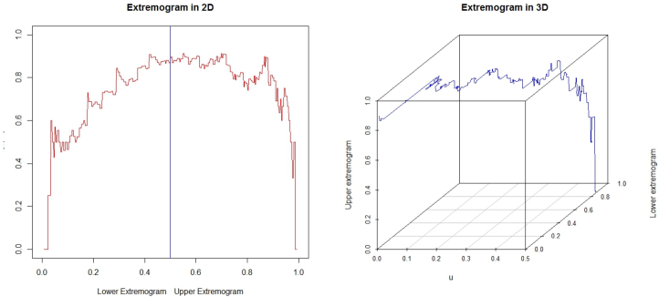
Figure 3: Graph of theoretical Extremogram .

This figures gives the representation in $2D$ and $3D$ for $A=(-\infty,1)$ and $A=(1,+\infty)$. We denote by upper extremogram for $A=(1,+\infty)$ and lower extremogram for $A=(-\infty,1).$ above the figure.

The following subsection gives a relation between the cross-extremogram and the copula function.

4.3 Cross-extremogram sampling with Spatial copulas

The following result provides a characterization of the cross extremogram in a copula contex, for two given sites $s_{i}$ and $s_{j}$.

Theorem 12

For two given sites $s_{i}$ and $s_{j}$ separated by $h_{ij}$, the extremal coefficient it given by:

$$\rho_{AB}(h_{ij})=1-\lim_{(u_{1i},u_{2j})\rightarrow(1^{-},1^{-})}\frac{u_{2j}-C_{h_{ij}}(u_{1i},u_{2j})}{1-u_{1i}}.$$ (33)

Proof. Let $F_{ji}(Z(x_{i}))=U_{ji}$ be the univariate distribution functions obtained by integral transforms to the variables $Z_{j}(x_{i})$ with $x_{j}-x_{i}=h_{ij},1\leq i,j\leq n,i\neq j$. It is well known that

$$\rho_{AB}(h_{ij})=\lim_{z\rightarrow\infty}P\left(Z_{2}(s_{j})\in zB/Z_{1}(s_{i})\in zA\right).$$

Since $A=(a,\infty)$ and $B=(b,\infty)$, it follows that

$$\rho_{AB}(h_{ij})=\lim_{z\rightarrow\infty}P\left(Z_{2}(s_{j})\in zB/Z_{1}(s_{i})\in zA\right).$$

It follow that,

$$\rho_{AB}(h_{ij})=\lim_{z\rightarrow\infty}P\left(Z_{2}(s_{j})\geq bz/Z_{1}(s_{i})\geq az\right).$$

So,

$$\rho_{AB}(h_{ij})=\lim_{z\rightarrow\infty}\frac{P\left(Z_{2}(s_{j})\geq bz,Z_{1}(s_{i})\geq az\right)}{P\left(Z_{1}(s_{i})\geq az\right)}.$$

$$\rho_{AB}(h_{ij})=\lim_{z\rightarrow\infty}\frac{\hat{H}_{h_{ij}}(bz,az)}{P\left(Z_{1}(s_{i})\geq az\right)}$$

with $\hat{H}_{h_{ij}}(bz,az)$ the survival function of the variables $Z_{2}(s_{j})$ and $Z_{1}(s_{i}).$

Moreover, if $C_{h_{ij}}$ is the jointed copula underlying the distribution of $Z_{1}(s_{i})$ and $Z_{2}(s_{j})$, then, it follows that:

$$\hat{H}_{h_{ij}}(bz,az)=1-F_{1i}(az)-F_{2j}(bz)+H_{h_{ij}}(bz,az)=1-F_{1i}(az)-F_{2j}(bz)+C_{h_{ij}}(F_{2j}(bz),F_{1i}(az)),$$

Likewise

$$P\left(Z_{1}(s_{i})\geq az\right)=1-P\left(Z_{1}(s_{i})<az\right)=1-F_{1i}(az).$$

By replacing these two last relations in (28), we obtain the following result:

$$\rho_{AB}(h_{ij})=\lim_{z\rightarrow\infty}\frac{1-F_{1i}(az)-F_{2j}(bz)+C_{h_{ij}}(F_{1i}(az),F_{2j}(bz))}{1-F_{1i}(az)}.$$ (34)

Let us consider $u_{1i}=F_{1i}(az)$ et $u_{2j}=F_{2j}(bz)$. When $z\longrightarrow+\infty$ then $u_{1i}\longrightarrow 1^{-}$ and $u_{2j}\longrightarrow 1^{-}.$ By using these transformations in the relation (34), it follows that:

$$\rho_{AB}(h_{ij})=\lim_{(u_{1i},u_{2j})\rightarrow(1^{-},1^{-})}\frac{1-u_{1i}-u_{2j}+C_{h_{ij}}(u_{1i},u_{2j})}{1-u_{1i}}.$$

So

$$\rho_{AB}(h_{ij})=1-\lim_{(u_{1i},u_{2j})\rightarrow(1^{-},1^{-})}\frac{u_{2j}-C_{h_{ij}}(u_{1i},u_{2j})}{1-u_{1i}}.$$

Hence the result (33) as disserted   

The following results provides an asymptotic statement.

Proposition 13

Consider $F_{ij}(az)=u_{ij}\in[0,1]$ the distribution function of the variable $Z_{j}(x_{i})$. If $z\longmapsto+\infty$, then $u_{ij}\longmapsto 1^{-}$ The relation (36) is written according to the copula by the relation:

$$\left(\begin{array}[]{c}\rho_{AA}^{11}(h_{ij})\\ \\ \\ \rho_{BB}^{22}(h_{ij})\\ \\ \\ \rho_{AB}^{12}(h_{ij})\\ \\ \\ \rho_{BA}^{21}(h_{ij})\end{array}\right)=\left(\begin{array}[]{c}1-\displaystyle\lim_{u_{11}\rightarrow 1^{-}}\frac{u_{11}-C_{h_{ij}}\left(u_{11},u_{11}\right)}{1-u_{11}}\\ \\ 1-\displaystyle\lim_{u_{22}\rightarrow 1^{-}}\frac{u_{22}-C_{h_{ij}}\left(u_{22},u_{22}\right)}{1-u_{22}}\\ \\ 1-\displaystyle\lim_{(u_{11},u_{22})\rightarrow(1^{-},1^{-})}\frac{u_{22}-C_{h_{ij}}\left(u_{22},u_{11}\right)}{1-u_{11}}\\ \\ 1-\displaystyle\lim_{(u_{11},u_{22})\rightarrow(1^{-},1^{-})}\frac{u_{11}-C_{h_{ij}}\left(u_{11},u_{22}\right)}{1-u_{22}}\end{array}\right)$$ (35)

Proof. In matrix form, the extremogram and the crossed extremogram can be written, (see Muneya et al. [$18$]), for all $x,x+h\in\mathbb{R}^{d}$, such as,

$$\left(\begin{array}[]{c}\rho_{AA}^{11}(h)\\ \\ \rho_{BB}^{22}(h)\\ \\ \rho_{AB}^{12}(h)\\ \\ \rho_{BA}^{21}(h)\end{array}\right)=\lim_{z\rightarrow+\infty}\left(\begin{array}[]{ccc}P\left(Z_{1}(x+h)\in zA/Z_{1}(x)\in zA\right)&&\\ &&\\ P\left(Z_{2}(x+h)\in zB/Z_{2}(x)\in zB\right)&&\\ &&\\ P\left(Z_{2}(x+h)\in zB/Z_{1}(x)\in zA\right)&&\\ &&\\ P\left(Z_{1}(x+h)\in zA/Z_{2}(x)\in zB\right)&&\end{array}\right)$$ (36)

Consider $B=A=(a,+\infty)$. Z being stationary, let $u_{1i}=u_{1j}=u_{11}$. With these transformations the relation (33) is written in the form,

$$\rho_{AA}^{11}(h_{ij})=\displaystyle\lim_{u_{11}\rightarrow 1^{-}}\frac{1-2u_{11}+C_{h_{ij}}\left(u_{11},u_{11}\right)}{1-u_{11}}.$$

Hence the first expression of (35).

In the same way, let us consider that $A=B=(b,+\infty)$ and $u_{2j}=u_{2i}=u_{22}$, the relation (33) is written in the form,

$$\rho_{BB}^{22}(h_{ij})=\displaystyle\lim_{u_{22}\rightarrow 1^{-}}\frac{1-2u_{22}+C_{h_{ij}}\left(u_{22},u_{22}\right)}{1-u_{22}}.$$

Hence the second expression of (35).

Similarly for $A=(a,+\infty)$ and $B=(b,+\infty)$, let $u_{1i}=u_{1j}=u_{11}$ and $u_{2j}=u_{2i}=u_{22}$. The relation (33) is written in the form,

$$\rho_{AB}^{12}(h_{ij})=\displaystyle\lim_{(u_{11},u_{22})\rightarrow(1^{-},1^{-})}\frac{1-u_{22}-u_{11}+C_{h_{ij}}\left(u_{22},u_{11}\right)}{1-u_{11}}.$$

By swapping A and B, $u_{11}$ and $u_{22}$ will change location. So this new relationship is still written in the form,

$$\rho_{BA}^{21}(h_{ij})=\displaystyle\lim_{(u_{22},u_{11})\rightarrow(1^{-},1^{-})}\frac{1-u_{11}-u_{22}+C_{h_{ij}}\left(u_{11},u_{22}\right)}{1-u_{22}}.$$

Hence the third and fourth expressions of (35).   

The following section is used to characterize the asymptotic dependence of extremes through the extremogram.

4.4 Asymptotic dependence and extremogram model

Consider a random variable $T(x)$ of a spatial process $T=\left\{T(x),x\in\mathbb{R}^{d}\right\}$ of standardized marginalized $F_{T}(T(x))$ .

Theorem 14

Let $Z=\left\{Z(x),x\in\mathbb{R}^{d}\right\}$ be a spatial stationary process such that $Z(.)=\frac{-1}{\log(F_{T}(T(.)))}$ . The marginal distribution of $Z$ are Fréchet standard marginal. The extremogram of random field Z(.) in two sites $x,x+h\in\mathbb{R}^{d}$ is define such as,

$$\rho_{AA}(h)=\mathcal{L}_{h}(u)(u)^{1-\frac{1}{\eta_{h}}};$$ (37)

where $\eta(h)\in(0,1]$ is the tail dependence coefficient, $A=(a;\infty)~{}~{}with~{}~{}a\in(0,1]$ and $\mathcal{L}(.)$ a slowly varying function.

Before giving the proof of the above theorem, let’s note that, even in a spatial study, there no loss of generality in dealing with Fréchet marginal, for any continuous function f, the transformation $f\left(Y_{i}\left(x\right)\right)=\frac{-1}{\log\left(Y_{i}\left(x\right)\right)}$ gives approximatively this distribution. Indeed, the parameters of the GEV in (2) as smooth function of the explanatory variables (longitude, altitude, elevation etc.) such as:

$$Y\left(x\right)=\mu\left(x\right)+\frac{\sigma\left(x\right)}{\xi\left(x\right)}\left[Z\left(x\right)^{\xi\left(x\right)}-1\right]~{}~{}where~{}~{}Z\left(x\right)\sim~{}Unit-Fr\'{e}chet,$$

for some partially correlation. That needs to model both spatial behaviour of marginal parameters and spatial joint dependence.

Proof. Considering $A=(a;\infty),a\in(0;1]$, the extremogram is written

$$\rho_{AA}(h)=\lim\limits_{z\rightarrow+\infty}\frac{P(Z(x+h)>az,Z(x)>az)}{P(Z(x)>az)}.$$

According to Ledford and Tawn $[16]$, when z tends towards infinity,

$$P(Z_{2}>r,Z_{1}>r)\sim\mathcal{L}(r)(r)^{1-\frac{1}{\eta}}.$$ (38)

Using (38), for any spatial process Z at two sites $x$ and $x+h$ when z tends towards infinity, we can write

$$P(Z(x+h)>az/Z(x)>az)\displaystyle\sim\mathcal{L}_{h}(az)(az)^{1-\frac{1}{\eta_{h}}}.$$ (39)

Thus, let $F(Z(x))$ be the distribution function of $Z(x)$ and $F(Z(x+h))$ the distribution function of $Z(x+h)$. According to the above, when z tends towards infinity, it follows that:

$$P(F(Z(x+h))>F(az)/F(Z(x))>F(az))\sim\mathcal{L}_{h}(az)(az)^{1-\frac{1}{\eta_{h}}}.$$ (40)

Considering $U=F(Z(x))$, $V=F(Z(x+h))$ and $u=F(az)$, it follows that:

$$P(V>u/U>u)\sim\mathcal{L}_{h}(u)(u)^{1-\frac{1}{\eta_{h}}},$$ (41)

when z tends towards infinity.
Using (41) in the expression of the extremogram, it follows that:

$$\rho_{AA}(h)=\mathcal{L}_{h}(u)(u)^{1-\frac{1}{\eta_{h}}}$$

Hence (37) as disserted   

Ancona and Tawn $[2]$ proposed a measure of extreme dependence called extreme variogram. This measure of dependence is expressed as a function of the dependence of tail by the relation:

$$\gamma_{E}(h)=2(1-\eta(h)).$$ (42)

Thus, the extremogram is modeled according to the extreme variogram by the following result.

Corollary 15

Let $\gamma_{E}(h)$ be the extreme variogram of two stationary random variables. The extremogram is linked to the extreme variogram by the relation:

$$\rho_{AA}(h)=\mathcal{L}_{h}(u)(u)^{-\frac{\gamma_{E}(h)}{2-\gamma_{E}(h)}};$$ (43)

with $\gamma_{E}(h)\in[0;2)$

Proof. From the relation (42), we can say that $\eta(h)=1-\frac{1}{2}\gamma_{E}(h).$. Using this relation in (37), it follows that:

$$\rho_{AA}(h)=\mathcal{L}_{h}(u)(u)^{1-\frac{2}{2-\gamma_{E}(h)}}.$$

Hence the expression,

$$\rho_{AA}(h)=\mathcal{L}_{h}(u)(u)^{\frac{-\gamma_{E}(h)}{2-\gamma_{E}(h)}}.$$

 

In the following, we estimate the extremogram using the relation (37). In this relationship, estimation of the extremogram requires estimation of the slowly varying function and the tail dependence coefficient. The following result gives the estimate of the extremogram.

Proposition 16

Consider two spatial random variables $Z(x)~{}and~{}Z(x+h);~{}x,~{}x+h\in\mathbb{R}^{d}$ of respective marginal distribution function $F_{Z}(Z(x))~{}and~{}F_{Z}(Z(x+h))$ . Let W$(.)$ considering

$$W(h)=\min\left\{\frac{-1}{\log\left(F_{Z}(Z(x)\right)};\frac{-1}{\log\left(F_{Z}(Z(x+h)\right)}\right\},$$

the estimated extremogram is written, for a fixed threshold $u_{h}$, in the form,

$$\hat{\rho}_{AA}(h)=\hat{c}_{h}(u)(u)^{1-\frac{1}{\hat{\eta}(h)}}.$$ (44)

Where

$$\hat{c}_{h}(u)=\frac{n_{u_{h}}}{n}u_{h}^{\frac{1}{\hat{\eta}(h)}}~{}~{}~{}~{};~{}~{}~{}~{}\hat{\eta}(h)=\frac{1}{n_{u_{h}}}\sum_{k=1}^{n_{u_{h}}}\log\left\{\frac{\hat{w}_{k}(h)-u_{h}}{u_{h}}\right\},$$

with $\hat{w}_{k}(h),k=1,\dots,n_{u_{h}}$ are the observations $\hat{W}(h)$ exceeding the threshold $u_{h}$.

Proof. The extremogram is expressed by the relation,

$$\rho_{AA}(h)=\lim\limits_{z\rightarrow+\infty}\frac{P(Z(x+h)>z,Z(x)>z)}{P(Z(x)>z)}=\lim\limits_{z\rightarrow+\infty}\frac{P(W(h)>z)}{P(Z(x)>z)}.$$

Ledford $([15];~{}[16])$ proposed to consider $\mathcal{L}_{h}(u)$ as constant that is,$\mathcal{L}_{h}(u)=c_{h}$ for all values z exceeding the threshold $u_{h}$. Using the observations of the independent replications of the spatial process approximate independent observations on $\hat{W}(h)$ are obtained, where $\hat{W}(h)$ is the approximation to the variable $W(h)$. From model (40) and n independent observations, the log-likelihood is

$$l(c_{h},\eta_{h})=(n-n_{u_{h}})\log\left(1-\frac{c_{h}}{u_{h}^{1/\eta_{h}}}\right)+n_{u_{h}}\log\left(\frac{c_{h}}{\eta_{h}}-c_{h}\right)-\frac{1}{\eta_{h}}\sum_{i=1}^{n_{u_{h}}}\hat{w}_{i}(h),$$

where $\left\{\hat{w}_{i}(h)\right\},i=1,\dots,n_{u_{h}}$ are the observations of $\hat{W}(h)$ above the threshold $u_{h}$. Using the maximum likelihood method, the estimate of $c_{h}$ is written,

$$c_{h}=\frac{n_{u_{h}}}{n}u_{h}^{\frac{1}{\hat{\eta}(h)}},$$

and using the Hill estimator method, the estimate of $\eta_{h}$ is written,

$$\hat{\eta}(h)=\frac{1}{n_{u_{h}}}\sum_{k=1}^{n_{u_{h}}}\log\left\{\frac{\hat{w}_{k}(h)-u_{h}}{u_{h}}\right\}.$$

Where $\hat{w}_{k}(h),k=1,\dots,n_{u_{h}}$ are the observations $\hat{W}(h)$ exceeding the threshold $u_{h}$. Hence the result,

$$\hat{\rho}_{AA}(h)=\hat{c}_{h}(u)(u)^{1-\frac{1}{\hat{\eta}(h)}}.$$ (45)

 

5 Conclusion and Discussion

In this study, we have been modeling some technical tools of spatial prediction within a copula-based space.  Thus, the extremal coefficient and the extremogram have been expressed via the underlying copulas. These results are important insofar as we want to determine the inter-site distribution dependence of a definite area.

The results of this paper make it possible to find a relation between the extremal coefficient and the extremogram using  the copula function. These new model are very crucial since the copula is a parametrization of  nomber of variables which do not deal with the marginal distribution. Hence, they allow not only to determine the distributional dependence of spatial or temporal extremes, but also, and above all, the conditional distributional dependence between these extremes in various observation sites.

References

• [1] A.C.Davison, R.Huser.E.Thibaud,”Geostatistics of Dependence and Asymptotically Independent Extremes", Math Geosci(2013) 45:511-529, DOI 10.1007/s11004-013-9469-y
• [2] Ancona-Navarrete, M.A., Dependence modelling and spatial prediction for extreme values, PhD Thesis, Lancaster University, Lancaster, 2000.
• [3] Basrak, B., Davis, R.A.and Mikosch.T.(2002). ”A Characterization of Multivariate Regular Variation. Ann.Appl.pro.12,908-20.
• [4] Beirlant, J., Goegebeur, Y., Segers, J. and Teugels, J. (2004) "Statistics of Extremes: Theory and Applications". John Wiley & Sons, Hoboken. Print ISBN:9780471976479, Online ISBN:9780470012383, DOI:10.1002/0470012382.
• [5] Beirlant J., Goegebeur Y, Segers J. and Teugels,J. (2005). Statistics of Extremes: theory and application, Wiley, Chichester, England.
• [6] Bondar, I., McLaughlin, K., & Israelsson, H. (2005). Improved Event Location Uncertainty Estimates, 27th Seismic Research Review, 299-307
• [7] Bordossy, A. (2006). Copula based geostatistical models for groundwater quality parameters. Water Resources Research 42.
• [8] Cooley D. Poncet P. and P. Naveau (2006). Variograms for max-stable random .elds. In Dependence in 8 Probability and Statistics. Lecture Notes in Statistics 187 373.390. Springer, New York
• [9] Diakarya Barro, Blami Koté and Soumaïla Moussa. "Spatial stochastic framework for sampling time parametric max-stable processes", International Journal of Statistics and Probability, vol. 1, no. 2, p. 203, 2012. DOI :10.5539/ijsp.v1n2p203.
• [10] Diakarya Barro, Saliou Diouf and Blami Koté (2012). Geostatistical Analysis with Conditional Extremal Copulas- International Journal of Statistics and Probability. Vol. 1, no. 2, pp 244-249. http://dx.doi.org/10.5539/ijsp.v1n2p244
• [11] Diakarya Barro, Simplice Doussou-Gbété, Saliou Diouf, "Stochastic Dependence Modelling Using Conditional Elliptical Processes", (2012) Journal of Mathematics Research; Vol. 4, No. 6 pp: 130-138 http://dx.doi.org/10.5539/jmr.v4n6p130.
• [12] Dossou-Gbete Simplice, Blaise Somé and Barro Diakarya (2009). Modelling the Dependence of Parametric Bivariate Extreme Value Copulas - Asian Journal of Mathematics & Statistics. Vol 2, Issue3, pp: 41-54 DOI: 10.3923/ajms.2009.41.54.
• [13] Fabrice Ouoba, Barro Diakarya, Hay Yoba Talkibing - Geostatistical Analysis with Copula-based Models of Madograms, Correlograms and Variograms - European Journal of Pure and Applied Mathematics 12 (3), 1052-1068. https://doi.org/10.29020/nybg.ejpam.v12i3.3389.
• [14] G. Frahm - On the extremal dependence coefficient of multivariate distributions.Statistics & Probability Letters 76(14):1470-1481 DOI:10.1016/j.spl.2006.03.006
• [15] H. Kazianka, J. Pils, Copula-based geostatistical modeling of Continuous and discrete data including Covariates", Stoch Environ Res Risk Assess (2010) 24:661-673, DOI. 101007/s 00477-009-0353-8
• [16] Joe, H.(1997),”Multivariate Models and Dependence Concepts ,” Chapman & Hall, London.
• [17] Ledford, A.w.and Tawn, J.A.,”Modelling dependence within joint tail region ,” J.R. Statist. Soc.B 59,475-499, (1997).
• [18] Ledford, A.w.and Tawn, J.A.,”Statistics for near independence in multivariate extreme values,” Biometrika 83,16-187,(1996).
• [19] Martin Larsson and Sidney I.Resnick, Long-Range Tail Dependence: EDM vs.Extremogram, w 911NF-07-1-0078 at Cornell University.
• [20] Muneya matsui and Thomas Mikosch,”The Extremogram and the Cross-Extremogram for a bivariate Garch (1,1) process",doi.10.1017/apr.2016.51
• [21] Richard A. Davis and Thomas Mikosch (2009). The extremogram: A correlogram for Extreme Events, November 13, 2008
• [22] Xavier Emery,”Géostatistique linéaire", Ecole des Mines de Paris, Centre de Géostatistique, 35,rue Saint Honoré , 77 305 Fontainebleau Cedex, France
• [23] Yong Bum Cho and Richard A. Davis, Department of statistics, Columbia University Souvik GHOSH, Asymptotic Properties of the Empirical Spatial Extremogram. Scandinavian Journal of statistics doi: 10.1111/sjos.12202