Understanding the high-mass binary black hole population from stable mass transfer and super-Eddington accretion in bpass

Abstract

With the remarkable success of the LVK consortium in detecting binary black hole mergers, it has become possible to use the population properties to constrain our understanding of the progenitor stars’ evolution. The most striking features of the observed primary black hole mass distributions are the extended tail up to $100\text{M}_{\odot}$ and an excess of masses at $35\text{M}_{\odot}$. Currently, isolated binary population synthesis have difficulty explaining these features. Using the well-tested bpass detailed stellar binary evolution models to determine mass transfer stability, accretion rates, and remnant masses, we postulate that stable mass transfer with super-Eddington accretion is responsible for the extended tail. These systems are able to merge within the Hubble time due to more stable mass transfer at higher donor masses with higher mass ratios and spin-orbit coupling allowing the orbits to shrink sufficiently. Furthermore, we find that in bpass the $35\text{M}_{\odot}$ excess is not due to pulsational pair-instability, as previously thought, but a feature caused by stable mass transfer, whose regime is limited by the mass transfer stability, quasi-homogeneous evolution, and stellar winds. These findings are at odds with those from other population synthesis codes but in agreement with other recent studies using detailed binary evolution models.

1 Introduction

In the years following the first observed binary black hole (BBH) merger in 2015, the number of observations has increased dramatically to a total of 76 BBH mergers with the release of Gravitational Wave Transient Catalogue 3 (GTWC-3; Abbott et al. 2021). This growing population is a window into the stellar physics governing the life and death of their progenitors. However, due to the million to billion year lifetimes, direct observation of their evolution is impossible. Therefore, population synthesis is used to probe the origins of merging BBH systems (see Mandel & Broekgaarden, 2021, and references therein) with the assumed evolutionary physics leaving imprints on the primary remnant mass, spin, and mass ratio distributions of the merging BBH population. However, GWTC-3 has shown that the BBH population is not yet well understood with the observed primary black hole (BH) mass ($\text{M}_{\text{1,BH}}$) distribution extending up to $100\text{M}_{\odot}$ - beyond the expected maximum (Heger & Woosley, 2002; Woosley et al., 2002; Woosley, 2017; Farmer et al., 2019; Renzo & Zapartas, 2020; Woosley & Heger, 2021; Mehta et al., 2022; Farag et al., 2022) - and an excess at $35\text{M}_{\odot}$ that is not connected to the turn-off of the distribution. From an isolated binary evolution perspective, the shape of this distribution is mostly influenced by the supernova and mass transfer prescriptions.

Depending on the supernova prescription, the primary remnant mass distribution can be drastically different (Mandel et al., 2020; Shao & Li, 2021; Ghodla et al., 2022b) with pulsational pair-instability supernovae (PPISN) and pair-instability supernovae (PISN) leaving the largest imprint on the distribution at high black hole masses (Spera & Mapelli, 2017; Marchant et al., 2019; Stevenson et al., 2019). These processes take place when extremely massive stars ($\text{M}_{\text{ZAMS}}\gtrsim 70\text{M}_{\odot}$; $\text{M}_{\text{He}}\gtrsim 30\text{M}_{\odot}$) enter a high-temperature, low-density regime in their core allowing for electron-positron pair production. At high core masses ($\text{M}_{\text{He}}\gtrsim 65\text{M}_{\odot}$), this leads to a single pulsational that completely disrupts the star, the PISN, and leaves no remnant behind (Fowler & Hoyle, 1964; Rakavy & Shaviv, 1967; Heger & Woosley, 2002). At smaller core masses, pulsational pair-instability drives mass ejection of the star through multiple pulsations. Eventually, the stellar structure exits the high-temperature, low-density regime and the star continues to evolve normally until it undergoes a core-collapse supernova. The supernova occurring after a pulsational pair-instability phase are referred of which the progenitors have experienced pulsational pair-instability are referred to as PPISN. As a consequence of the mass ejection, a large range of Zero-Age Main-Sequence (ZAMS) masses converge to a narrow range of helium core masses between $35-50\text{M}_{\odot}$ (Woosley, 2017). Depending on the remnant mass prescription, these result in similar BH masses and a pile-up before an absence of them due to PISN (Heger & Woosley, 2002; Woosley et al., 2002; Stevenson et al., 2019; Marchant et al., 2019; Farmer et al., 2019). It is, therefore, expected that a pile-up is associated with a cut-off in the primary BH mass distribution. Since more massive stars ($\text{M}\gtrsim 260\text{M}_{\odot}$; $\text{M}_{\text{He}}\gtrsim 140\text{M}_{\odot}$ ) completely collapse into a BH, the pair-instability disruption creates a gap in the isolated BH mass distribution, also know as the ’upper mass gap’ or ’PISN mass gap’. The lower edge of this gap is at $\text{M}_{\text{BH}}\approx 50\text{M}_{\odot}$ (see Woosley & Heger, 2021, and references therein). This limit can be raised using rapid rotation (Marchant & Moriya, 2020; Woosley & Heger, 2021) or altering the nuclear reaction rates (Woosley & Heger, 2021; Mehta et al., 2022; Farag et al., 2022) to include more massive BHs, which have been observed in the PISN mass gap, such as GW190521. However, the pile-up mass from PPISN increases as well, further decreasing the association with the observed excess at $35\text{M}_{\odot}$.

Without altering the stellar physics, such massive BBH merger could also be explained by non-isolated binary formation pathways (Yang et al., 2019; Rodriguez et al., 2019; Santoliquido et al., 2020; Di Carlo et al., 2020; Renzo et al., 2020b; Mapelli et al., 2021; Bouffanais et al., 2021; Zevin et al., 2021; Arca-Sedda et al., 2020, 2021; Costa et al., 2022; Ballone et al., 2022; Banerjee, 2022). Each would leave imprints on the properties of the merging BBH population and could challenge the standard isolated binary evolution formation pathway.

Another possibility for the existence of BHs in the PISN mass gap is mass transfer onto the BH from a companion (van Son et al., 2020; Woosley & Heger, 2021). This occurs when the radius of the star, the donor star, expands beyond its Roche Lobe Radius and, thus, mass is transferred to the companion, the accretor. This can drastically alter the mass ratios and evolution of the star with the stability and the accretion efficiency determining the outcome of this mass transfer.

If the radius of the donor star contracts or remains constant as a response to mass loss during the Roche Lobe Overflow (RLOF), the mass transfer is stable. If, on the other hand, the star expands as a response to mass transfer, the positive feedback-loop results in the donor star engulfing the whole system in a Common Envelope (CE) phase (Paczynski, 1976; Webbink, 1984; Iben & Livio, 1993; Podsiadlowski, 2001; Ivanova et al., 2013), where part or all of the envelope is removed from the system. The accretion onto the BH during the CE phase is limited (De et al., 2020), but RLOF before and/or after the CE can result in accretion onto the BH and its effects is poorly explored for high-mass stars.

Systems undergoing CE are, currently, considered the main formation channel for merging BBH systems (Dominik et al., 2012; Belczynski et al., 2016; Bavera et al., 2021; Zevin et al., 2021; Zevin & Bavera, 2022; van Son et al., 2022) with only the high-mass primary mass systems being formed through stable mass transfer (SMT) (Neijssel et al., 2019; van Son et al., 2022). However, stable mass transfer (SMT) has been shown to play a more important role than previously thought with accretion being more stable in detailed stellar models than those used in rapid population synthesis (Marchant et al., 2021; Gallegos-Garcia et al., 2021; Klencki et al., 2021), like compas (Riley et al., 2022), startrack (Belczynski et al., 2016), mobse (Giacobbo et al., 2018), and cosmic (Breivik et al., 2020) which use stability criteria based on the evolutionary phase of the star from Hurley et al. (2002). Using improved stability criteria Olejak et al. (2021) has shown that more stable mass transfer takes place in startrack. While this results in an extended primary BH mass range up to $55\text{M}_{\odot}$, it is unable to predict more massive primary mass BHs.

Super-Eddington accretion onto the BH during SMT could allow the primary BH to gain a significant amount of mass to become a PISN mass gap BH (van Son et al., 2020). However, for SMT systems to merge within the Hubble time, they need to lose angular momentum to reduce the size of their orbit. With Eddington luminosity limited accretion, this happens through mass loss from the system during RLOF, but this does not occur for super-Eddington accretion and BHs in the PISN mass gap are unable to merge within the Hubble time (van Son et al., 2020; Bavera et al., 2021; Zevin & Bavera, 2022). Thus, most BBH population synthesis codes limit the accretion onto the BH to the Eddington luminosity. On the other hand, super-Eddington accretion onto a BH is a candidate for Ultra Luminous X-ray sources (Woosley & Heger, 2021) and is theoretically possible (Sądowski & Narayan, 2016; Woosley & Heger, 2021)

Since the high end of the primary BH mass distribution is not yet well understood, we predict the properties of the BBH population using detailed stellar models. These models from bpass (Eldridge et al., 2017; Stanway & Eldridge, 2018) allow for super-Eddington accretion onto a BH and modelling of the response of the donor star to the mass loss without relying on parameterisation for this response. In combination with the star formation history and metallicity evolution from the state-of-the-art TNG-100 simulation, we predict the primary mass and mass ratio distributions of the merging BBH population, and compare them against the observed population. In Section 2, we discuss bpass, its prescription for mass transfer stability and efficiency, remnant mass, and PPISN prescription. We present our results in Section 3, where explore the formation pathways of the merging BBH systems and describe the formation of features matching observation in the high BH mass range in Section 4. In Section 5, we discuss how the stability criteria of mass transfer create this outcome. We look at the impact from (P)PISN and quasi-homogeneous evolution on the $\text{M}_{\text{1,BH}}$ distribution and its features, in Section 6. In Section 7, we discuss how this relates to the current view and what limitations our predictions have. We present our conclusions in Section 8.

2 Method

2.1 Population synthesis

To calculate the number of merging BBH systems within the Hubble time, we use the detailed stellar models and population synthesis of Binary Population Synthesis And Spectral Synthesis (bpass) v2.2.1 (Eldridge et al., 2017; Stanway & Eldridge, 2018). Here, we will give a short overview of relevant mechanics and changes compared to previous work (Eldridge et al., 2019; Tang et al., 2020; Briel et al., 2022). We implement improvements made by Ghodla et al. (2022b) to rejuvenation and the merger time calculation and use the cosmological star formation history from the TNG100-1 simulation (Springel et al., 2018; Nelson et al., 2018; Pillepich et al., 2018; Naiman et al., 2018; Marinacci et al., 2018), as in Briel et al. (2022). We use the cosmological parameters from Aghanim et al. (2020) ($h=0.6766$, $\Omega_{\text{M}}=0.3111$, and $\Omega_{\Lambda}=0.6889$).

bpass is a population synthesis suite that uses a grid of $\sim 250,000$ 1D theoretical stellar models that include single and binary evolution and contains 13 metallicities mass fractions ranging from $10^{-5}$ to $0.04$. It uses a custom version of the Cambridge stars code (Eggleton, 1971), and is described in Eldridge et al. (2008); Eldridge et al. (2017) and Stanway et al. (2018). It implements metallicity dependent wind mass loss rates from de Jager et al. (1988), Vink et al. (2001) for OB stars and Nugis & Lamers (2000) for hydrogen depleted Wolf-Rayet stars.

The fiducial bpass v2.2.1. population is weighted using initial binary parameters from Moe & Di Stefano (2017) and a Kroupa (2001) initial mass function extended up to $300\text{M}_{\odot}$. This has been tested against a wealth of observables and can self-consistently reproduce a number of massive star evolutionary characteristics, young and old stellar populations (Eldridge & Stanway, 2009; Wofford et al., 2016; Eldridge et al., 2017; Stanway & Eldridge, 2018), and transients rates (Eldridge & Stanway, 2016; Eldridge et al., 2019; Tang et al., 2020; Ghodla et al., 2022b; Briel et al., 2022).

bpass implements a unique method in evolving binary systems to reduce computational time. Before the first supernova, the primary star is evolved in detail using the adapted STARS code (Eggleton, 1971), while the secondary star is evolved using the single star rapid evolution equations from Hurley et al. (2002). This is know as the primary model. After the fate of the primary star has been determined and a natal kick has been applied, a secondary model is selected and the secondary star is evolved in detail, either as a single star or as a binary with a compact object, contingent on the outcome of the primary. If the secondary has accreted more than 5 per cent of its initial mass and has a metallicity fraction of 0.004 or below, the secondary model is, instead, replaced by a quasi-homogeneous model (QHE). We explore a more detailed accretion QHE prescription by Ghodla et al. (2022a) in Section 6.1. Once the secondary also reaches the end of its life, its fate is determined and a natal kick is applied again. If the system is still bound, and contains two compact objects, the coalescence time is calculated using Peters (1964). We define this as the merger time of the system, while the delay time includes the lifetime of the progenitor stars before the formation of the secondary BH.

2.2 Remnant mass prescription

In the fiducial bpass population, the remnant mass is determined by calculating the remaining bound mass after injecting $10^{51}$ erg into the star while taking into account its internal structure (Eldridge & Tout, 2004). The remnant receives a natal kick from a Maxwell-Boltzmann distribution with $\sigma=265$ km s^-1 (Hobbs et al., 2005) for masses below $3\text{M}_{\odot}$ and is otherwise reduced by a factor $\text{M}_{\text{remnant}}/1.4\text{M}_{\odot}$. Per model we sample 1000 kicks from this distribution to cover the effects of the supernova on the binary.

While the standard bpass output does contain a PISN prescription Woosley et al. (2002), it does not contain a PPISN prescription. This process, however, is essential in determining the BBH population (Stevenson et al., 2019; Marchant et al., 2019; Broekgaarden et al., 2021), as its thought to result in the upper mass gap and a pile-up of events. For this work, we implement the prescription from Farmer et al. (2019) based on the CO core of the progenitor, while keeping the standard bpass prescription in the other regimes. Since no upper limit based on the CO core is currently available (for an overview of limits see Woosley & Heger, 2021), we use the upper limit based on the He core mass from Woosley et al. (2002). This results in the prescription in Equation 1, which transitions smoothly between regimes, as shown in Figure 1.

$$\text{M}_{\text{CO}}<38\ \text{M}_{\odot}\longrightarrow \>10^{51}\text{erg injection}$$

$$38\ \text{M}_{\odot}\leq\text{M}_{\text{CO}}<60\ \text{M}_{\odot}\longrightarrow$$ Farmer et al. (2019)

$$\text{M}_{\text{CO}}\geq 60\ \text{M}_{\odot}\text{ and }\text{M}_{\text{He}}<133\ \text{M}_{\odot}\longrightarrow \>\text{M}_{\text{rem}}=0$$

$$\text{M}_{\text{He}}\geq 133\ \text{M}_{\odot}\longrightarrow \>10^{51}\text{erg injection}$$ (1)

Figure 1 shows the relation between CO core and remnant masses for the primary and secondary models resulting in BBH mergers. In Section 6.2, we explore the effect of the Fryer et al. (2012) prescriptions and (P)PISN on the $\text{M}_{\text{1,BH}}$ distributions. Furthermore, we change baryonic masses into gravitational masses, following (Fryer et al., 2012) with $\text{M}_{\text{grav}}=0.9\text{M}_{\text{bar}}$ for remnant masses above $3\text{M}_{\odot}$ and for masses below we use

$$\text{M}_{\text{grav}}=2\frac{\sqrt{1+3\text{M}_{\text{bar}}-1}}{3}$$ (2)

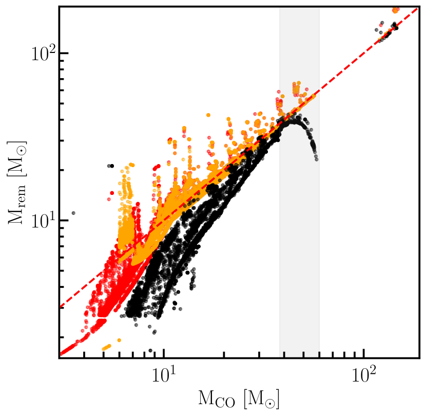
Figure 1: The remnant mass over the CO core for the primary and secondary models at their formation resulting into BBH mergers at $z=0$ using the prescription used in this work (black), and the Rapid (orange) and Delayed (red) prescriptions from Fryer et al. (2012). At $\text{M}_{\text{CO}}>11$, the Fryer et al. (2012) are similar and overlap. The PPISN regime is marked in grey. We indicate where the remnant is the same size as the carbon-oxygen core (red dashed line). Section 6.2.1 discusses the impact of the Fryer et al. (2012) prescriptions on the $\text{M}_{\text{1,BH}}$ distribution.

2.3 Mass transfer

Mass transfer is one of the most important effects in binary evolution with about 50-70 per cent of massive stars experiencing it during their lifetime (Sana et al., 2012, 2013). Determining the stability of this mass transfer is challenging, because it requires detailed modelling of the structure of the star to determine its response to the mass loss $\zeta=\text{d}\log R/\text{d}\log M$. To this end, rapid population synthesis codes use approximations for this response based on the evolutionary phase of the star (Belczynski et al., 2020; Olejak & Belczynski, 2021; Riley et al., 2022). However, bpass uses detailed stellar models that calculate the equations describing the stellar interior in a time resolved manner, thus we directly model the response of the donor radius, which leads to significant differences in the donor response (Woods & Ivanova, 2011; Pavlovskii & Ivanova, 2015). When a star fills its Roche Lobe, mass is transferred based on the amount of overflow according to Hurley et al. (2002):

$$\dot{\text{M}}_{\text{d}}=F(\text{M}_{\text{d}})[\ln(\text{R}_{\text{d}}/\text{R}_{\text{RL}})]^{3}\text{M}_{\odot}\text{yr}^{-1}$$ (3)

$$\text{with }F(\text{M}_{\text{d}}) =3\times 10^{-6}[\text{min}(\text{M}_{\text{d}},5.0)]^{2}$$ (4)

Equation 3 shows the mass loss rate from the donor star with its mass as $\text{M}_{\text{d}}$, and its radius and Roche Lobe radius as $\text{R}_{\text{d}}$ and $\text{R}_{\text{RL}}$, respectively. The material in this process can be accreted by a companion star, but it is limited to $\dot{\text{M}}_{\text{a}}\leq\text{M}_{\text{a}}/\tau_{KH}$, where $\text{M}_{\text{a}}$ is the mass of the accretor star. A compact object below $3\text{M}_{\odot}$ (Chamel et al., 2013) is limited to the Eddington luminosity, as per (Cameron & Mock, 1967). The accretion is unrestricted for masses above this limit, since the accretion onto a BH is uncertain and multiple methods for super-Eddington accretion have been proposed Wiktorowicz et al. (see 2015, and references therein). Additional material is lost to the system with its angular momentum by treating this as a wind from the donor star.

When RLOF takes place, we also consider tidal forces due to the interaction. Due to tidal locking, they can spin up the components of the binary using angular momentum of the orbit, which can result in significant orbital shrinkage depending on the properties of the binary. In some cases, a runaway effect causes the system to merge, also known as the Darwin Instability (Darwin, 1879).

If, due to the response of the donor star to mass loss or due to the tidal interactions, the donor star radius expands past the orbital separation of the system, we assume a CE takes place (for a more detailed description of our CE prescription, see Stevance et al. in prep.). In our CE prescription, we remove mass from the star as quickly as the detailed model allows, and relate the binding energy of the material lost to the orbital energy. This process conserves angular momentum, takes into account the structure of the stars, and does not require the envelope to be completely stripped. However, it results in longer duration CE phases, albeit still significantly shorter than the thermal timescale of the stars and should not influence the predictions of the binary evolution (Eldridge et al., 2017). Once the radius shrinks below the orbital separation the CE phase ends. Our CE treatment is close to the $\gamma$ formalism (Nelemans et al., 2000; Nelemans & Tout, 2005) due to the angular momentum conservation, as reported in Stevance et al. (in prep.), and we retroactively calculate the $\alpha_{\text{CE}}\lambda$ from our detailed models for comparison against the $\alpha\text{-}\lambda$ formalism used in rapid population synthesis codes (Ivanova et al., 2013). This results in equivalent values for $\alpha_{\text{CE}}\lambda$ ranging from 3 to 30 (Eldridge et al. 2017; Stevance et al. in prep.). Since $\alpha_{\text{CE}}$ is a free parameter based on the conversion efficiency of binding energy to orbital energy and $\lambda$ a parameter to determine how the structure of the star affects the binding energy, we do not separate them. Before and after the CE phase, mass can be transferred onto the companion, but accretion is non-existent during the CE. Mass transfer continues until its radius shrinks to below the Roche Lobe radius.

3 Formation Pathways

3.1 Cosmic Merger Rate over Redshift

From the intrinsic properties of the merging BBH population of the GWTC-3 analysis, bpass can predict the total cosmic rate of BBH over redshift, the mass ratio distribution and primary mass distribution. In Figure 2, we show the redshift evolution of the BBH merger rate over redshift against the observed intrinsic rate from their power law + peak (PP) population model. It consists of an over-redshift-evolving merger rate power-law and a Gaussian. The predicted rate using the TNG-100 star formation history results in a lower rate than observations. However, it is important to keep in mind that the rate is not only dependent on the assumed physics, but also the cosmic star formation history, which can have drastic effects on the final calculated cosmic rate (Chruslinska & Nelemans, 2019; Neijssel et al., 2019; Santoliquido et al., 2021; Broekgaarden et al., 2021). We use the same population data, but use the empirical star formation history prescription from Briel et al. (2022), which uses the Madau & Dickinson (2014) star formation history and the Langer & Norman (2006) metallicity evolution, and find that the rate at $z=0$ aligns with observations. However, the evolution over redshift remains shallower than found by Abbott et al. (2021).

It is promising that the TNG-100 rate is below the observed rate, since our prediction only includes BBH mergers from isolated binary evolution. Other processes, such as triples and dynamic mergers, are likely to contribute to the observed rate, which are absent in our prediction. These could add at least 30 per cent to the total BBH observed rate (Zevin et al., 2021). However, care should be taken with formation channel predictions due to uncertainties in star formation and stellar physics (Broekgaarden et al., 2021).

The current TNG-100 BBH merger rate is lower than reported in Briel et al. (2022), which is due to the improved merger time calculation and the treatment of rejuvenation during mass transfer, as described in Ghodla et al. (2022b). The latter provides a smoothing of the BBH delay time distribution, while the former generates more accurate merger time predictions. Together, these improvements increase the merger time for some systems and, thus, reduce the BBH mergers within the Hubble time. We report the BBH, black-hole neutron-star, and binary neutron star merger rates at $z=0$ in Table 1 for completion. Except for the BBH rate, these align with current observational constraints from Abbott et al. (2021).

	BBH	BHNS	BNS
	[yr-1 Gpc-3]
Predicted	6.5	27.0	93.1
Abbott et al. (2021)	10 – 130	7.4 – 320	13 – 1900

Table 1: The compact object rates at $z=0$ for the TNG-100 star formation history. The observed rates from Abbott et al. (2021) are the combined 90 per cent confidence intervals for their models for the non-evolving and redshift evolving merger rates.

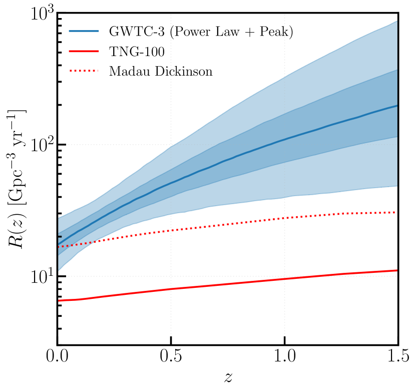
Figure 2: The predicted evolution of the intrinsic BBH merger rate (red solid) over redshift using the TNG-100 cosmic star formation history compared to found evolution found by Abbott et al. (2021) using their over redshift evolving PP model (blue) with 50 per cent (dark blue) and 90 per cent (light blue) credible bounds. The BBH merger rate using the Madau & Dickinson (2014) cosmic star formation history (red dashed) with the same BBH population as TNG100 is shown to indicate the error from the star formation history.

3.2 Population Properties

More understanding can be gained from the properties of the population. While observations are still limited, one has to be cautious drawing strong conclusions from these comparison, but the most constraint observables from GWTC-3 are the primary mass and mass ratio distribution. In Figure 3 we compare the predicted population against the intrinsic observed population from the pp model from Abbott et al. (2021). We split the $\text{M}_{\text{1,BH}}$ space into 40 logarithmic spaced bins between 2 and 200 $\text{M}_{\odot}$. Unless otherwise stated we use this binning for all $\text{M}_{\text{1,BH}}$ distributions. In Appendix A, we perform a Poisson error calculation, bootstrap sampling, and apply a kernel density function to determine the uncertainty associated with this distribution, which is limited.

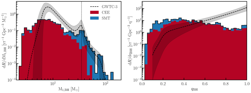
Figure 3: The event rate density over the primary BH mass (left) and the mass ratio (right) at $z=0$ with the results from the PP model from Abbott et al. (2021) as the dashed line. The gray area is the 95 per cent confidence interval. The presence of a common envelope in the evolution of the BBH merger progenitor has been marked with red, while blue indicated that no common envelope has taken place and only stable mass transfer has occurred during the life of the BBH progenitor system. The vertical dotted line indicates the $35\text{M}_{\odot}$ BH mass. $\mathrm{q}_{\mathrm{BH}}$ is split into 40 linear bins between 0 and 1.

While the predicted rate over mass ratio with $q_{\text{BH}}=\text{M}_{\text{2,BH}}/\text{M}_{\text{1,BH}}$, where $\text{M}_{\text{2,BH}}$ is the mass of the secondary BH in Figure 3 does increase rapidly at low $q_{\text{BH}}$, it does not continue to increase with increasing $q_{\text{BH}}$ and instead drops beyond $q_{\text{BH}}\sim 0.4$. This might be due to our CE prescription, which dominates the mass ratio distribution, or the remnant mass prescription (for the latter, see Section 6.2).

Although the mass ratio distribution does not agree with the observed values, we find good agreement in the high-mass regime of the $\text{M}_{\text{1,BH}}$ distribution between our predictions and GWTC-3. The predicted distribution contains a double peak structure with a peak near $5\text{M}_{\odot}$ and $35\text{M}_{\odot}$ with the latter agreeing with observations. Moreover, it extends into the PISN mass gap with masses over $100\text{M}_{\odot}$, as shown in Figure 3. However, it does over predict the low mass BBH mergers ($\text{M}_{\text{1,BH}}\lesssim 5\text{M}_{\odot}$) and underestimates the number of systems near $10\text{M}_{\odot}$.

The well-matched nature of the predictions to observations in the high BH mass regime raises questions about the formation of the high-mass BHs and their merger time. Moreover, the peak at $35\text{M}_{\odot}$ seems to be disconnected from the turn-off of the $\text{M}_{\text{1,BH}}$ distribution, as observed; this calls into question its connection to PPISN, which is thought to lead to a pile-up at the end of the primary BH mass distribution near $\sim 40-50\text{M}_{\odot}$ (Marchant et al., 2019; Renzo et al., 2020a; Woosley & Heger, 2021). Because these questions are linked, the Section 4 will cover these components in detail, but here we will discuss the formation channels giving rise to the $\text{M}_{\text{1,BH}}$ distribution.

To this end, we tag BBH merger progenitor model that undergo CE during their evolution as CEE, and models that only experience SMT as SMT. If multiple mass transfer phases take place during the evolution, we check if any of them is unstable, if so we tag the model as undergoing CEE. If no interactions take place, the model is tagged as NON. We perform the tagging for the primary and secondary models.

In Figure 3, we separate the $\text{M}_{\text{1,BH}}$ distribution into a formation channel with a CE in their evolution, and in a pure SMT sample, that only contains systems (primary and secondary models) with stable mass transfer. We find that high-mass BH ($20-115\text{M}_{\odot}$) are increasingly formed through systems only undergoing SMT, which is in agreement with Neijssel et al. (2019) and van Son et al. (2022). The majority of these events have mass ratios below $q_{\text{BH}}<0.4$.

To see what models these systems come from, Figure 4 shows that the main channels contributing to the SMT only channel are SMT+SMT with SMT in the primary and secondary model, and SMT+NON, where after SMT in the primary model no interaction in the secondary model takes place. Both channels originate from massive stars ($\text{M}_{\text{1,ZAMS}}>60\text{M}_{\odot}$) with a slightly less massive companion ($\text{M}_{\text{2,ZAMS}}>35\text{M}_{\odot}$). This is further motivated by the central figure, which shows the fraction of events going through a formation pathway at a given $\text{M}_{\text{1,ZAMS}}$ and $\text{M}_{\text{2,ZAMS}}$. While these systems originate from similar populations, they undergo drastically different evolution. The NON+SMT systems only contribute 0.30 per cent to the total merging BBH rate, but originate from a wide variety of initial masses.

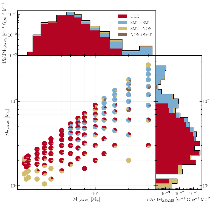
Figure 4: The ZAMS distributions of $M_{1}$ and $M_{2}$ for systems leading to a BBH merger at $z=0$. The SMT channel has been split into its individual formation channels, since it dominates the high $\text{M}_{\text{1,BH}}$ regime. Each circle contains the systems at those $\text{M}_{\text{1,ZAMS}}$ and $\text{M}_{\text{2,ZAMS}}$ and are split into their formation pathways, weighted according to the systems weight w.r.t. total weight at this $\text{M}_{\text{1,ZAMS}}$ and $\text{M}_{\text{2,ZAMS}}$. $\text{M}_{\text{1,ZAMS}}$ is split into 16 bins, which are the ZAMS masses in the bpass grid. $\text{M}_{\text{2,ZAMS}}$ is split into 40 bins between 2 and 300 $\text{M}_{\odot}$.

Nearly all BBH merger progenitor systems interacted during their lifetime and the CE and SMT channel result in different remnant mass outcomes. Figure 5 shows the period evolution separated per evolutionary phase and mass transfer case. In the left column, i.e. the evolution of the binary before the first supernova where the primary star, $\text{M}_{1}$, initiates mass transfer, while the right column shows the period evolution of the secondary binary models, where the initial primary star has become a compact object and the secondary star, $\text{M}_{2}$, fills its Roche Lobe. Throughout the evolution we keep the definition of the primary (1) and secondary (2) the same, as such in the primary (secondary) models $\text{M}_{1}$ is $\text{M}_{\text{d}}$ ($\text{M}_{\text{a}}$) and $\text{M}_{2}$ is $\text{M}_{\text{a}}$ ($\text{M}_{\text{d}}$).

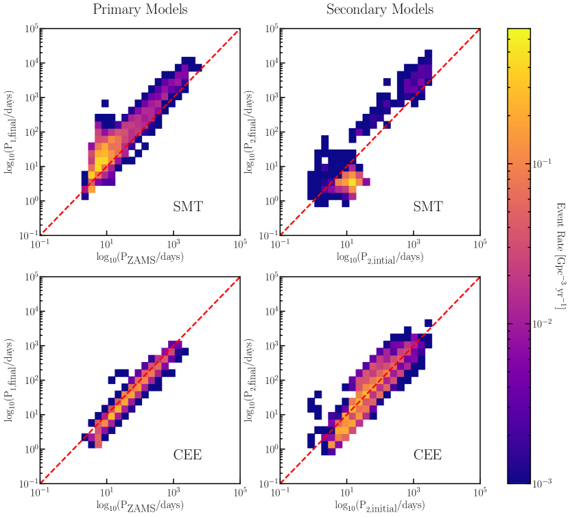
Figure 5: The period evolution of the merging BBH progenitors. The left column contains the primary binary models in the simulation, i.e. the evolution before the primary supernova. The right column contains the secondary binary models after the first supernova. The x-axis represents the period at the start of the model. This means that the P in the left column represents the ZAMS period of the systems. They y-axis represents the period at the end of the model evolution, which does not include the SN. Between the primary (left) and secondary (left) binary models the remnant mass prescription is applied to the primary star. The primary ($1$) and secondary ($2$) stars defined at the beginning of the evolution and we do not change this definition throughout the evolution. The final mass ratio is not the BBH mass ratio, since the remnant mass prescription still needs to be applied to the secondary star. The rows are split between SMT and CEE taking place in this model. The periods are logarithmic binned in 30 bins between $10^{-1}$ and $10^{5}$., The dashed red line indicates that the period has remained unchanged throughout the evolution, e.g. $\text{P}_{\text{initial}}=\text{P}_{\text{final}}$.

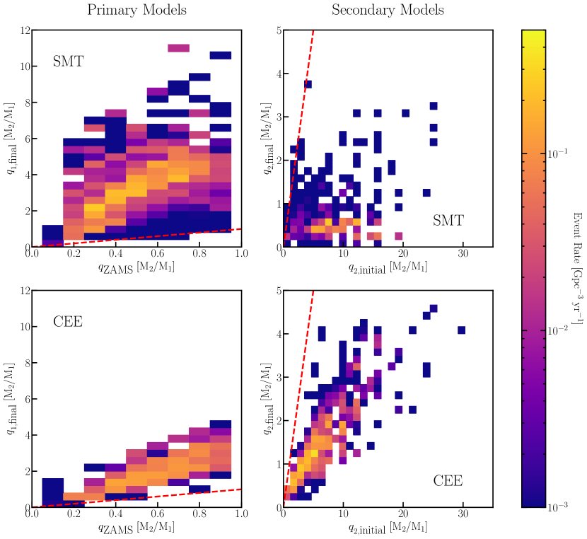
Figure 6: Same as Figure 5, but for the mass ratio. Depending on the $q$ value the binning is different. The $q_{\text{ZAMS}}$ bins are centred around the $q$ values used by bpass, 0.1 to 0.9 with steps of 0.1. $q_{\text{1,final}}$, $q_{\text{2,initial}}$, and $q_{\text{2,final}}$ each contains 30 bins linearly spaced between $0\text{--}12$, $0\text{--}35$, and $0\text{--}5$, respectively. The dashed red line indicates that the period has remained unchanged throughout the evolution, e.g. $q_{\text{initial}}=q_{\text{final}}$.

In the initial phase of the evolution (left), we see that SMT (top) leads to larger periods and, thus larger separations than systems experiencing CEE (bottom). This is a result of material being transferred from the more initially massive star to the less massive in the system. At the start of mass transfer, this results in an orbit shrinkage, but once the mass ratio becomes more equal the orbit starts to widen (Soberman et al., 1997; van Son et al., 2020).

Looking at the mass ratio evolution of SMT systems during the primary phase of the binary evolution in Figure 6 (top left), we see that the mass ratios flip and increase up to $q_{\text{1,final}}=\text{M}_{2}/\text{M}_{1}=11$ when the primary star dies, with most systems laying between 2 and 6. The CEE channel (bottom left) is only able to achieve a maximum mass ratio of $q_{\text{1, final}}=5$ with most models between 0.5 and 4, but does reduce the periods for most systems, as expected.

The remnant mass prescription further increases the mass ratio up to $q_{\text{2, i}}=30$ by reducing the primary mass, as can be seen in the right column in Figure 6. This column contains the secondary models split between those experiencing SMT and CE, thus, a model in SMT could have experience SMT, CE, or not interacted in the primary model. Most of the systems undergoing only SMT after the first supernova have an initial mass ratios between $5<q_{\text{2,i}}<20$. A few low contributing systems have more extreme mass ratios up to $q_{\text{2, i}}=25$, which are unexpected in the context of SMT and we will explore these further in Section 5.2. Eventually, the mass transfer stops and the systems reach mass ratios between 0 and 1, which will be further reduced by the remnant mass prescription. Thus, super-Eddington accretion on to the BH leads to a mass reversal, such that the $\text{M}_{\text{1,ZAMS}}$ also becomes $\text{M}_{\text{1,BH}}$. This results in limited mass ratio reversal (Zevin & Bavera, 2022; Broekgaarden et al., 2022; Mould et al., 2022), as will be discussed in Section 7.3.

The common envelope in the second phase of the systems evolution decreases the mass ratio linearly, e.g. a higher initial mass ratio leads to a higher final mass ratio. Since we tag a system as CEE if the undergoes a single CE phase during the phase of the systems evolution, we do not identify multiple mass transfer phases in the system, which occur in our model. Therefore, phases of SMT in a system undergoing CE can alter the mass ratio and periods.

In general, systems experiencing only SMT in the secondary model, have on average smaller periods at the end of the model than those that have experienced CE. The reason for the orbital shrinkage depends on the binary model parameters, but most shrinkage is caused by tidal synchronisation reducing the angular momentum in the orbit. Most systems are below the critical mass ratio for the Darwin Instability ($q>12$) (Eggleton, 2011), but those above are able to avoid it due to rapid changes in the mass ratio (Stȩpień, 2011), the rapid shrinkage of the donor radius, and/or increased winds due to high helium surface abundance. We further discuss the stability of these models in Section 5.

The right column of Figure 5 shows that the period change in during the CEE interaction spreads out its original distribution and reduces the period for systems with period $\lesssim 10^{1.5}$. The SMT channel reduces the period of such systems more significantly than the CEE channel. Furthermore, two main clusters of period can be identified around $10^{1}$ and around $10^{3}$ with limited systems in between these period. This is a result of interaction on the Hertzsprung gap being mostly unstable and will be discussed more in Section 5. However, both channels have systems with final periods that are unable to merge when assuming a circular orbit, e.g. $10^{4}$ days. We find that these systems come from higher metallicity populations, and have eccentricities near unity due to the natal kick they received, as such they are able to merge within the Hubble time. This shows that it is possible to get BBH systems merging within the Hubble time, even when considering super-Eddington accretion, while retaining a significant amount of mass, thus resulting in more massive BBH systems.

We further separate the formation pathways per metallicity and per evolutionary model in Figure 7. The highest contribution comes from the SMT+CEE (45.24 per cent), where the primary model only experiences SMT and the secondary contains a CE phase. The next largest formation channel is CEE+CEE (31.17 per cent) channels, where a CE takes place in both the primary and secondary model. The dominance of CE in the formation of merging BBHs is in agreement with other population synthesis codes (Dominik et al., 2012; Belczynski et al., 2016; Bavera et al., 2021; Zevin et al., 2021; Zevin & Bavera, 2022; van Son et al., 2022). The SMT+CEE distribution contains mergers originating from a variety of metallicities, but lower mass primary mass systems originate from higher metallicities than the higher primary mass systems due to the mass loss from stellar winds. The CEE+CEE distribution, on the other hand, has a higher contribution from low metallicity star formation. Following these high contributing events is the SMT+NON channel, where the binary only interacts before the first supernova (6.95 per cent). This distribution is dominated by mergers from low metallicity ($Z<0.006$) star formation with a large contribution between 30 to 40 $\text{M}_{\odot}$ from $Z=0.0001$. While this channel contains the largest primary BH mass, most other events are constrained to $\text{M}_{1}<40\text{M}_{\odot}$. The next largest formation pathway, the CEE+NON channel (6.79 per cent), is also limited to $\text{M}_{1}<40\text{M}_{\odot}$ and low metallicity. Similarly, CEE+SMT only occurs at low metallicity, but has a specific mass regime (15 to 55 $\text{M}_{\odot}$) and only contributes 0.08 per cent. The events only interacting in the primary preferentially come from low metallicity events, while systems interacting only in the secondary phase originate from higher metallicity environments. The SMT+SMT channel (6.55 per cent) forms most of the high primary mass BH systems, similar to the distribution shown by van Son et al. (2022). We note a metallicity dependence in the primary mass with low primary mass BHs originating from higher metallicity environments, as a result of the formation pathway discussed in Section 4.1.

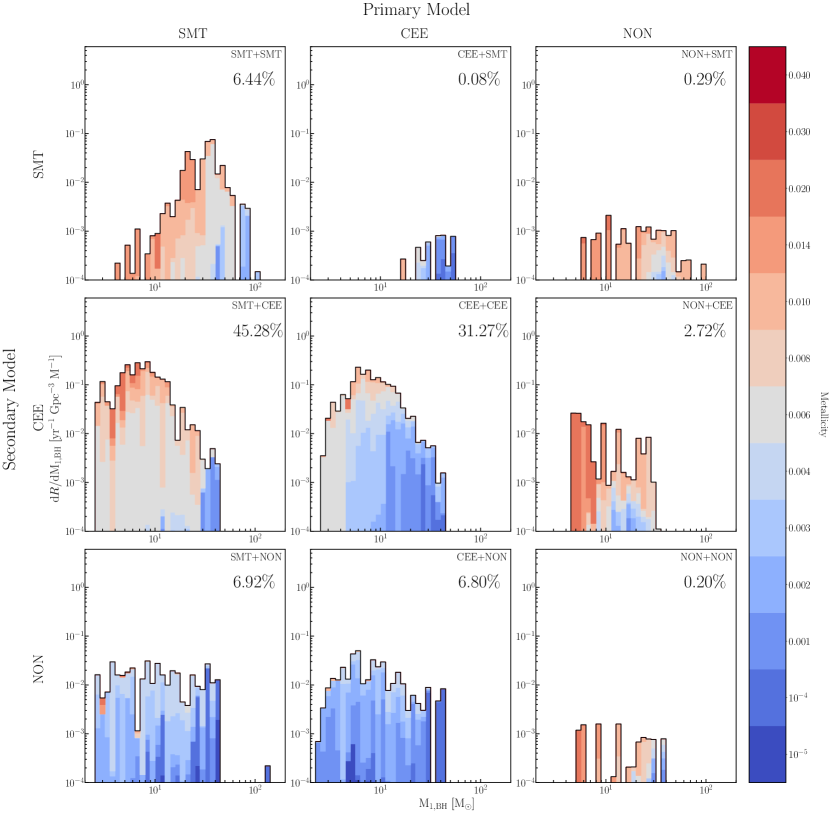
Figure 7: The predicted event rate at $z=0$ over primary BH mass separated by formation channels coloured by the metallicity at which the binary system was formed. The column are split based on only SMT, CEE, or NON occurring in the primary model, as described in Section 3.2. The rows are the same, but for the secondary models. The percentages is the contribution of that formation channel to the total BBH merger rate.

4 Primary remnant mass distribution features

Mass transfer is a defining feature for the outcome of the binary system and stable mass transfer leads to higher mass systems. We find a distribution that matches the high-mass properties of the observed intrinsic primary mass distribution. These are the extended mass range and an excess at $35\text{M}_{\odot}$. In the next sections, we cover these two findings in more details.

4.1 The $35\text{M}_{\odot}$ Excess

In Figure 3, we find an excess of systems near M${}_{1}\approx 35\text{M}_{\odot}$, similar to observations, which previously has been attributed to a pile-up of PPISN events. We tag the systems undergoing PPISN and find that only the high end of the peak is a result of the PPISN.

As shown in Figure 8, the majority of $\sim 35\text{M}_{\odot}$ BH progenitors do not experience PPISN. Instead, we find that the peak consists of systems only undergoing SMT with PPISN being present around $40\text{M}_{\odot}$ bin. The CEE channel, on the other hand, has a decreasing rate until $35\text{M}_{\odot}$, after which it slightly increases due to PPISN events. Since other population synthesis codes are dominated by CEE systems, the pile-up is logically attributed to PPISN. However, since in this mass regime bpass is dominated by SMT, this is not the main formation process for the $35\text{M}_{\odot}$ peak.

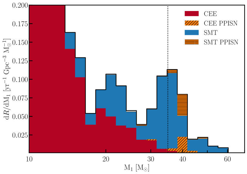
Figure 8: The primary remnant mass distribution at $z=0$ rebinned to 50 logarithmic spaced bins and zoomed in on the $35\text{M}_{\odot}$ excess, where the systems are split into the SMT and CEE channels with the PPISN tagged per channel. The systems experiencing PPISN are above $35\text{M}_{\odot}$ (dashed line). The majority of the peak if formed through the SMT channel. The black line represent the total event rate, which also contains non-interacting systems. An additional excess near $20\text{M}_{\odot}$ can be identified and is discussed in Section 7.4.

The main contributors to the $35\text{M}_{\odot}$ peak within the SMT channel are the SMT+SMT and SMT+NON formation pathways. These channels originate from massive stars ($M_{1}>60\text{M}_{\odot}$) with a slightly less massive companion ($M_{2}>35\text{M}_{\odot}$), as shown in Figure 4. While these systems originate from similar populations, they undergo drastically different evolution. Therefore, we look at each pathway separately in the following sections.

4.1.1 Single stable mass transfer only (SMT+NON)

Because these systems only interact before the first supernova, the first formed BH remains unchanged in mass after its formation and, thus, come from initially massive stars that have experienced or are close to the lower limit of PPISN.

The non-interacting nature after the first SN in this system makes sure that the primary BHs do not continue to grow after their formation. This is a result of the companion experiencing QHE which occurs in bpass when 5 per cent of its initial mass being accreted from the primary at low metallicities. This explains the low average metallicity of this channel in Figure 7, since QHE is limited to systems with a metallicity of 0.004 or below. The majority of systems in this channel undergo QHE. Our QHE models are assumed to be fully mixed during hydrogen burning, thus their mean molecular weight increases with the progression of nuclear burning. This leads to the radius of the star shrinking rather than expanding, as would occur with normal main sequence stars. Thus, QHE stars fail to fill their Roche Lobe and do not interact with their companion. The BH companion will be unable to grow further and PPISN systems only contribute to the high end of the peak near $35\text{M}_{\odot}$ through the SMT+NON formation channel.

4.1.2 Double stable mass transfer only (SMT+SMT)

The SMT+SMT formation pathway is more complicated than the SMT+NON channel due to interactions in multiple evolutionary phases. Similar to SMT+NON these merging BBHs come from very massive ZAMS stars, but they do not all experience PPISN.

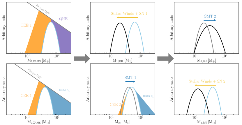
Figure 9: A cartoon depiction of the BBH distribution and the stellar physics that restricts stable mass transfer at low metallicity. The peaks represent the SMT channel at each stage. From the Kroupa IMF (grey), most systems do not result into a BH or merge within the Hubble time. In the primary models, the low ends of the $\text{M}_{\text{1,ZAMS}}$ and $\text{M}_{\text{2,ZAMS}}$ distributions are limited by mass transfer stability (CEE 1; orange), while the high-mass regime is limited by QHE (purple). As a result of limited high-mass contribution, the secondary is also limited (max q; blue). As metallicity increases, the $\text{M}_{\text{1,iBH}}$ shifts towards lower masses due to stellar winds. Also in the primary model, $\text{M}_{\text{2,ZAMS}}$ increases due to SMT onto it, resulting in the $\text{M}_{\text{2,i}}$ distribution. In the secondary model, CE restricts $\text{M}_{\text{2,i}}$ at the low end (CEE 2; orange), while the low end is limited by the maximum mass ratio. During this phase, $\text{M}_{\text{1,iBH}}$ increases in mass due to SMT to give the $\text{M}_{\text{1,BH}}$ distribution in the top right Figure. $\text{M}_{\text{2,i}}$ losses material due to SMT, stellar winds, and the supernova, and results in the $\text{M}_{\text{2,BH}}$ distribution in the bottom right Figure. Black and blue peaks lines peaks indicate the BH and stellar distribution, respectively. Gray distributions are the distributions from the previous phase.

Instead, limitations from mass transfer stability, QHE, and stellar winds restrict the SMT+SMT channel to form BHs around $35\text{M}_{\odot}$. We distinguish between the regime with QHE ($Z<0.006$) and without, because QHE restricts further interactions in bpass. Figure 9 shows a cartoon depiction of how each process in the QHE regime restricts the SMT+SMT formation pathway. Most low ZAMS primary and secondary masses will not form a BH or merge within the Hubble time.

At QHE metallicities, $\text{M}_{\text{1,ZAMS}}$ is restricted at the high end due to QHE (see Section 6.1 for more details). Due to the high masses, these models often interact stably and have a lot of material available for mass transfer. Since the timescales of the primary and secondary as similar (see Appendix B), accretion is efficient and the models are likely to undergo QHE. This restricts further interactions and makes it impossible for the QHE systems to merge within the Hubble time. As a result of the limited $\text{M}_{\text{1,ZAMS}}$, $\text{M}_{\text{2,ZAMS}}$ is also restricted, since we define $\text{M}_{\text{1,ZAMS}}>\text{M}_{\text{2,ZAMS}}$.

The low end of $\text{M}_{\text{1,ZAMS}}$ is limited by CE. If the donor star is less massive, it is more likely to undergo unstable mass transfer and, thus, does not contribute to the SMT channel (see Section 5 about the stability). Similarly if the companion star is too small compared to the primary mass, it will experience CE due to the large mass ratio and restricts the bottom of the secondary mass distribution.

Further limitations are introduced at later stages of the evolution. For example, the formation of the first BH, $\text{M}_{\text{1,iBH}}$, at the lowest metallicities is limited by the (P)PISN, creating a pile-up around $40\text{M}_{\odot}$. However, the contribution of these events is limited and at higher metallicities stellar winds limit the maximum $\text{M}_{\text{1,iBH}}$ mass. Furthermore, since the accretion before the first SN is limited due to QHE, the secondary mass distribution ($\text{M}_{\text{2,i}}$) is similar to the ZAMS distribution ($\text{M}_{\text{2,ZAMS}}$). The exception is that the low end is further restricted by the mass transfer stability of the interaction in the secondary model, e.g. low secondary mass stars are more likely to experience CE, while higher mass systems are more likely to interact stably. At low metallicity this results in mass ratios close to unity. As a result of these mechanism, low metallicity systems are at the PISN limit and have limited accretion.

As metallicity increases, mass transfer becomes more stable during the core-helium burning. Since the material available for mass transfer during this phase is limited, QHE can be avoided, while $\text{M}_{\text{2,i}}$ can still transfer a significant amount of material onto $\text{M}_{\text{1,iBH}}$. We discuss this further in Section 4.2.

At metallicities above $0.004$, QHE no longer restricts the maximum $\text{M}_{\text{1,ZAMS}}$. Instead it is restricted by the IMF, and higher mass primaries and secondaries can interact stably. This increases the systems contributing to the merger rate and the material available for the formation of BHs. At the same time, mass loss due to stellar winds has also increased, which decreases $\text{M}_{\text{1,iBH}}$ and $\text{M}_{\text{2,BH}}$. The interplay between the mass transfer and stellar winds results an initial increase in BH mass with increased metallicity till the stellar winds become stronger and reduce the BH mass again. Since mass is stored on the companion and transferred back onto the BH, a transition to BBH systems with high $\text{M}_{\text{1,BH}}$ and small $\text{M}_{\text{2,BH}}$ (q closer to 0) takes place, as metallicity increases.

We now turn our attention to the actual distributions in the SMT+SMT channel in Figure 10. The left most Figures shows that most of the systems originate from $Z>0.004$; above the QHE limit. While the contribution of systems below the QHE limit to the peak is limited, these systems play an important role in the high-end of $\text{M}_{\text{1,BH}}$ and will be discussed in Section 4.2.

Above the QHE limit, systems with $Z=0.006$ (grey) cover a large range of $50<\text{M}_{\text{1,ZAMS}}<300$. As metallicity increases (redder), the high end of $\text{M}_{\text{1,ZAMS}}$ becomes restricted due to stellar winds keeping the radius of the star small and limiting interactions. Furthermore, the material available for mass transfer and $\text{M}_{\text{1,iBH}}$ formation reduces. Thus, as metallicity increases $\text{M}_{\text{1,iBH}}$ decreases and the change in mass between $\text{M}_{\text{2,ZAMS}}$ and $\text{M}_{\text{2,i}}$ decreases.

The $\text{M}_{\text{1,iBH}}$ distribution after the first SN is similar to the single star remnants with the same ZAMS mass, but is more extended to the low and high end. The less massive BHs are due to enhanced mass loss, reducing the core mass of stars and leading to less massive remnants as discussed by Laplace et al. (2021). The more massive BHs are, however, more surprising, but were also found in Eldridge & Stanway (2016). These are a consequence of mass transfer preventing the opening of a convective zone at the edge of the helium core post-main sequence. This convective region would normally dredge-up core material decreasing its mass. By preventing its formation, the final core mass is greater than expected. This process is only revealed by the detailed evolution models.

With limited material available for the BH to grow during the second phase of SMT, $\text{M}_{\text{1,BH}}$ decreases with increasing metallicity. Due to this process, the $35\text{M}_{\odot}$ peak contains a metallicity distribution, where as $\text{M}_{\text{1,BH}}$ increases, metallicity decreases. The combination of stellar wind, QHE, and stability criteria result in the placement of this peak near $35\text{M}_{\odot}$. Furthermore, $\text{M}_{\text{2,i}}$ has additional mass loss at higher metallicity due to stellar winds. Due to which, $\text{M}_{\text{2,BH}}$ decreases and the mass ratio of the final BBH systems increases. Moreover, these systems are also formed more recently and most require eccentric orbits to be able to merge within the Hubble time.

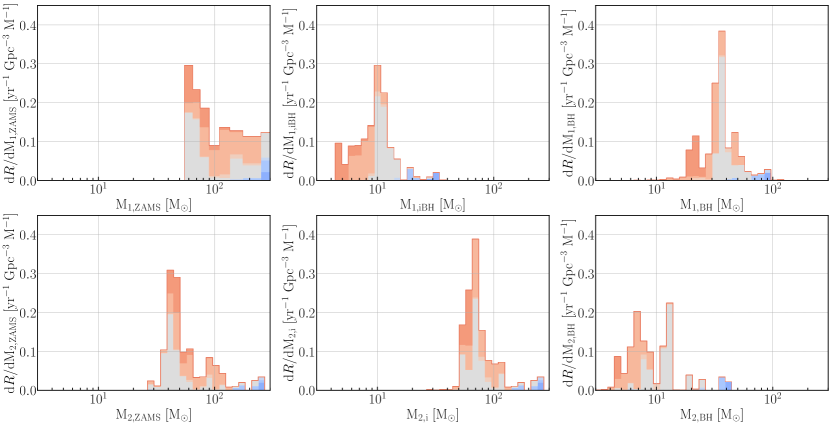
Figure 10: The evolution of the primary and secondary masses in the SMT+SMT channel separated by metallicity. Standard binning (40 bins) is used, except for $\text{M}_{\text{1,ZAMS}}$ for which we use the values of the bpass grid. The left most figures show the ZAMS distribution, the middle figures the masses right after the first supernova, and the right figures the final remnant masses of the merging BBHs in this channel.

4.2 The formation of upper mass gap BHs ($>50\text{M}_{\odot}$)

The formation of high-mass BH is difficult due to the PPISN and PISN mechanism reducing the BH progenitors mass or completely disrupting it, respectively. Furthermore, the formation of a common envelope will shed a significant amount of stellar material from the system, further reducing the available mass for BH formation. In agreement with Neijssel et al. (2019) and van Son et al. (2022), we find that high-mass BH ($20-115\text{M}_{\odot}$) are increasingly formed through systems only undergoing stable mass transfer, as shown in Figure 3. However, we find significantly higher masses than predicted by rapid population synthesis codes (Bavera et al., 2021; Olejak & Belczynski, 2021; van Son et al., 2022).

This is a direct result of super-Eddington accretion onto the BH, which results in no mass loss from the system during accretion, except for wind drive mass loss. However, van Son et al. (2020) and Bavera et al. (2021) have shown that a super-Eddington accretion rate onto a BH leads to fewer mergers within the Hubble time due to reduced mass and angular momentum loss from the system. Thus, for the systems to be able to merge, their periods need to shrink sufficiently during the systems evolution. This can either happen through angular momentum loss from the system, mass transfer from the more massive star to its companion, or tidal synchronisation. Since super-Eddington accretion limits the former, we focus our attention on the latter two.

The $\text{M}_{\text{1,BH}}$ distribution in Figure 7 shows that the high-mass BHs come from high-mass sub-QHE limit metallicity $\text{M}_{\text{1,ZAMS}}$ systems with massive $\text{M}_{\text{2,ZAMS}}$. During the initial phase of the evolution mass is transferred to the companion, but the amount transferred is limited, because QHE would limit further interactions, if accretion was more than 5 per cent of the companion mass. The formed $\text{M}_{\text{1,iBH}}$ is, therefore, limited by (P)PISN. As a result of the supernova, the systems have large mass ratios ($q_{\text{2,final}}\sim 5-10$). But because $\text{M}_{\text{2,i}}$ are massive, they are able to interact stably (see Section 5) and due to the interaction taking place on the main-sequence, a significant amount of material is transferred onto the BH.

Since the initial mass ratio was larger, mass is transferred from the most massive star to the less massive BH, which reduces the period. Furthermore, as a result of the high mass ratio, tidal forces are strong and further reduces the period. A CE is avoided by the ’fast’ radial shrinkage of the donor star, and the ’fast’ increase of the BH mass due to the super-Eddington accretion, as such the mass ratio approaches unity and the radius of the donor star does not reach the separation of the system. These interactions are on a longer than thermal timescale, although the thermal timescale is short due to the massive nature of the donor star.

5 Mass Transfer Stability

We have shown that using detailed stellar models with PPISN and super-Eddington accretion onto BHs leads to an extended mass tail up to $100\text{M}_{\odot}$ and an overdensity near $35\text{M}_{\odot}$, as observed by the LIGO/VIRGO/KAGRA collaboration. These are both an effect of increased stable mass transfer. As such, this section covers an overview of the nature of the detailed models, how the stability criteria influence the features in the $\text{M}_{\text{1,BH}}$ distribution, and a comparison against more detailed mass transfer stability determination. The Supplementary Material explores the stability of the primary and secondary models in bpass.

5.1 Nature of the envelope

As discussed in Section 2.3, a star can respond to mass loss by expanding or contracting, which depends on the properties of the envelope of the star. In general, if a star as a convective envelope it expands due to adiabatic mass loss, while it contracts if the envelope is radiative (Hjellming & Webbink, 1987; Soberman et al., 1997). However, work by Ge et al. (2010, 2015, 2020a, 2020b) has shown that metallicity, radius and evolutionary phase also influence the mass transfer stability. Most rapid population synthesis BBH merger predictions do not take this into account (startrack, mobse, cosmic, compas; Belczynski et al., 2016; Giacobbo et al., 2018; Breivik et al., 2020; Riley et al., 2022) and instead use an adiabatic model based on the evolutionary phase to determine the stability of mass transfer, as per Hurley et al. (2002). This leads to more unstable mass transfer, since, for example, convective envelope criteria are applied to core-helium burning stars that can have radiative envelopes (for an overview see Klencki et al., 2020; Klencki et al., 2021). Furthermore, other detailed mass transfer simulations have shown that BH-star systems are more likely to undergo SMT (Pavlovskii et al., 2017; Marchant & Moriya, 2020; Marchant et al., 2021), impact population of merging BBHs (Gallegos-Garcia et al., 2021), and that the donor response is very different than the simplified adiabatic model and holds across stellar codes (stars, mesa, Heyney-type code) (Woods & Ivanova, 2011; Passy et al., 2012).

Since bpass is based on the Cambridge stars code, stability is determined by following the equations of stellar structure through mass loss, which allows us to determine the nature of the envelope over a large mass and metallicity range. Since mass transfer alters the stellar evolution and the internal structure of the donor star, we turn our attention to single stars to determine the convective or radiative nature of the donor envelope, because this is the structure of the star just before the onset of RLOF. Section 1 in the Supplementary Material covers the evolution of the envelope over age, mass, and metallicity. We find that at nearly all massive stars spend their main-sequence with a radiative envelope. Post-Main Sequence the envelope depends on the initial mass and metallicity. At $Z>0.002$, $\textrm{M}_{\textrm{ZAMS}}\leq 26$ have convective envelopes after core-helium burning initiates. Figure 11 shows this for $Z=0.006$. Above this mass, the envelopes only have a short period of convection before core-helium burning initiates, after which the star has a radiative envelope, which is similar to results found by Klencki et al. (2021). This indicates that interactions during this phase are more stable than estimated by rapid population synthesis codes. Below $Z<0.002$, the star becomes convective during core helium burning at $\textrm{M}_{\textrm{ZAMS}}\geq 21$. Below this limit, the absence of metals restricts the formation of a convective envelope till late in the core-helium burning phase. At $Z=10^{-5}$, the convective zone is completely avoided at these low masses.

Figure 11: The radiative (blue) or convective (red) nature of the envelope of single stars at $Z=0.006$ from ZAMS to the end of Helium core burning. The process for extraction from the single star models is discussed in the Supplementary material. For models that did not reach the end of core helium burning, we interpolate between ZAMS masses. We indicate the ZAMS (solid black line) and the end of the Main-Sequence (dashed black line).

This shows that metallicity, age, and mass all influence the nature of the envelope in single star. In binaries, short mass transfer phases could alter the internal structure of the star in such a way that at later stages in the donors evolution the envelope no longer becomes convective. Thus, without detailed treatment of the internal structure at the moment of mass, BHs formed through SMT are missed in rapid population synthesis codes.

5.2 Mass Ratio Exploration

The resulting $q$ values for SMT onto the BH in Figure 6 are more extreme than typically found in detailed binary models (Marchant et al., 2021; Gallegos-Garcia et al., 2021). Although the mass ratios at the moment of mass transfer are less extreme, values up to $q=23$ remain. This could indicate that our determination for CE is too constricting, since our stability determination only considers the donor radius and the separation of the system. Thus, in this section, we explore how the high-mass features in $\text{M}_{\text{1,BH}}$ depend on the mass ratios and explore the extreme mass ratio systems.

5.2.1 Mass Ratio Cuts

Since the high-mass features predominantly come from the SMT+SMT channel, we perform two cuts at $q<10$ and $q<5$ based on the mass ratio at the moment of mass transfer onto the BH. The $q<10$ cut in Figure 12 shows that large mass ratios ($q>10$) are only a fraction of the SMT+SMT channel. Moreover, the cuts show that the $35\text{M}_{\odot}$ peak is dominated by $q<5$ systems with the spread around the peak being a result of more extreme mass ratios ($q<10$). As a consequence, the upper mass gap systems undergo SMT with mass ratios between 5 and 10, and the stability criteria could influence the existence of these systems. These mass ratios are larger than generally considered stable, but are not unreasonable at low metallicity and high donor mass. In Section 5.3, we compare our stability criteria other detailed work, and the Supplementary Material describes that these models are stable due the super-Eddington accretion and faster shrinkage of the donor star radius than the Roche Lobe.

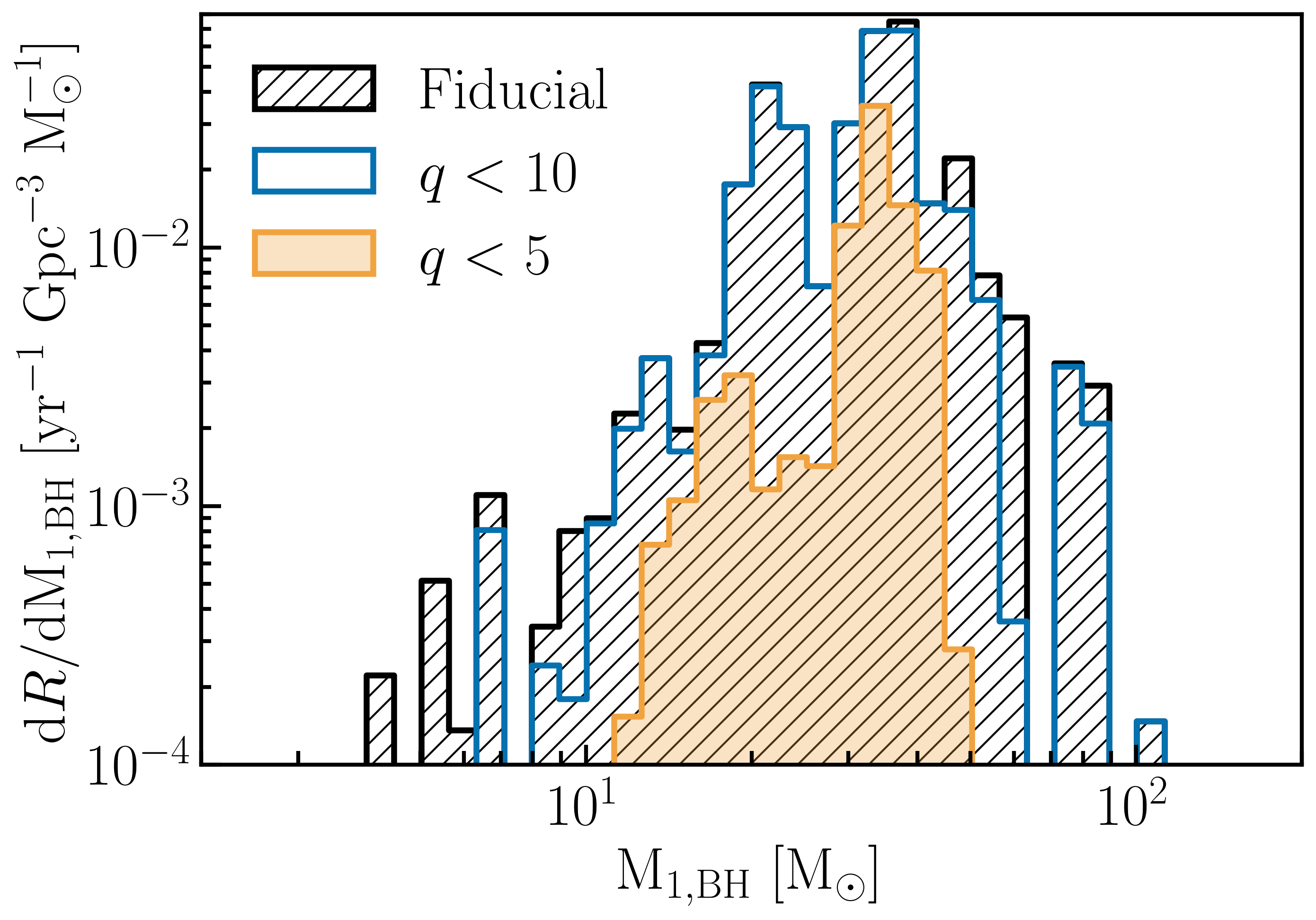
Figure 12: The primary BH mass ($\text{M}_{\text{1,BH}}$) distribution at $z=0$ from the SMT+SMT channel with the fiducial model (black) and two cuts based on the mass ratios at the moment of mass transfer with $q<10$ (blue) and $q<5$ (orange).

5.2.2 Extreme Mass Ratios

Some BH-star systems undergoing have extreme mass ratios with $q_{\text{2,initial}}$ up to 25, as shown in Figure 6. The actual mass ratio at the moment of RLOF is less extreme due to mass loss, but some $q>15$ remain. These systems all interact on the main-sequence and occur between a small BH (3-6 $\text{M}_{\odot}$) and a large star ($70\textrm{--}140\text{M}_{\odot}$) at $Z>0.01$, where stellar winds are strong. As a result, the primary loses mass quickly, while the amount of RLOF is small. This reduces the mass ratio and, thus, avoids the Darwin Instability. Due to the strong stripping of the star, stellar winds become stronger and limit further interactions. Although these systems exist, their contribution to the $\text{M}_{\text{1,BH}}$ distribution is minimal and limited to the low mass regime.

5.3 Comparison to the literature

Because some $q\approx 25$ systems undergo SMT and the $q\approx 5\textrm{--}10$ for the high-mass $\text{M}_{\text{1,BH}}$ is higher than conventional main-sequence interactions, we compare the bpass stability to other detailed analyses of the stability of mass transfer. In the Supplementary Material, we further describe the mass transfer stability in bpass.

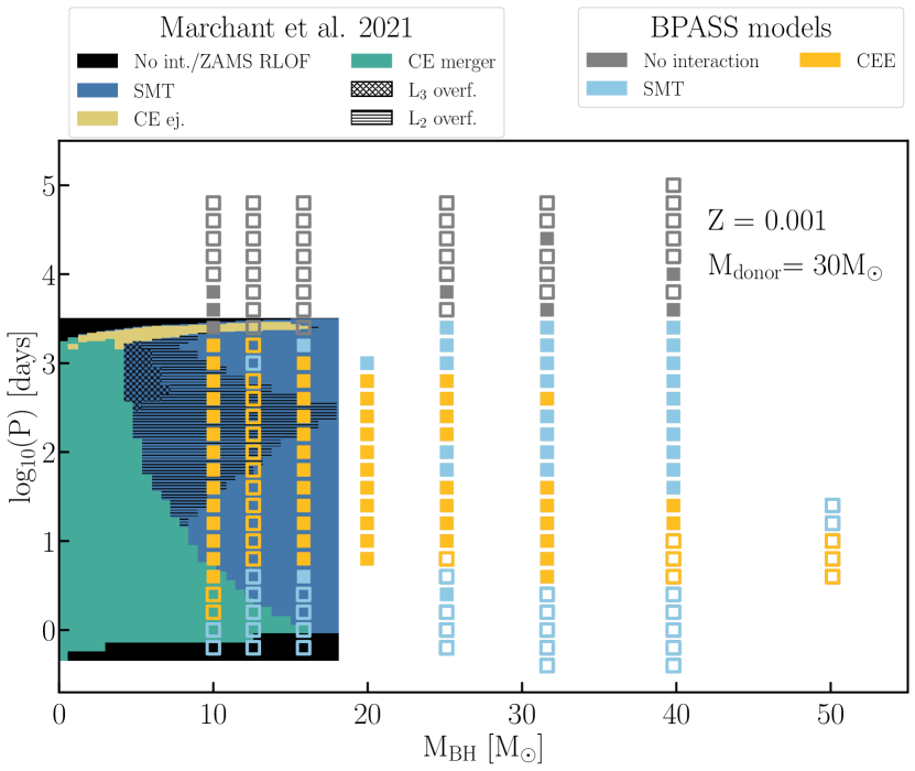
Figure 13: Mass transfer stability comparison between Marchant et al. (2021) models ($Z=0.00142$) and the BPASS models ($Z=0.001$). The Marchant et al. (2021) CE and SMT interactions leading to BBH mergers within the Hubble time have been grouped together to those taking longer. The solid squares mark the models contributing at the event rate at $z=0$, while the open squares do not contribute to the BBH merger rate.

Marchant et al. (2021) explored the stability of mass transfer using detailed treatment of the mass flow through $\textrm{L}_{1}$ and mass loss through the outer Lagrangian point of the donor star ($\textrm{L}_{2}$/$\textrm{L}_{3}$) using mesa (Paxton et al., 2011; Paxton et al., 2013, 2015, 2018, 2019) at a metallicity of $Z=0.00142$ and a $\text{M}_{\text{d}}=30\text{M}_{\odot}$. Figure 13 shows their results with overlapped the stability of the bpass models at the closest metallicity ($Z=0.001$) at $M_{\textrm{donor}}=30\text{M}_{\odot}$.

Although the overlap between the simulations is limited, bpass contains CE in regions where SMT is predicted by Marchant et al. (2021). This is most likely due to the synchronisation of the donor spin with the orbit when RLOF takes place, which shrinks the orbital separation and in general leads to more frequent CE, which is not considered in Marchant et al. (2021). Interestingly, non of the CE interaction at this metallicity and mass in bpass lead to a merger, but they do not probe far into the CE merger regime from Marchant et al. (2021).

In bpass SMT occurs pro-dominantly during the main-sequence and during core-helium burning, when the envelope of the donor star is radiative and the star evolves on a nuclear timescale. When the mass ratio is reversed ($\text{M}_{\text{d}}\lesssim\mathrm{M}_{\mathrm{BH}}$), the system can interact stably during the Hertzsprung gap at $Z=0.001$ and donor mass. However, the stability during this phase is highly dependent on the donor mass, metallicity, and mass ratio (see Supplementary Material).

A larger donor mass range using similar stellar evolution was explored by Gallegos-Garcia et al. (2021) at $Z=0.00142$. As with Marchant et al. (2021), we find that more CE takes place due to the tidal forces, and that more SMT takes place on the main-sequence. Furthermore, similar to Gallegos-Garcia et al. (2021), we find that for higher donor masses, the stability on the main-sequence increases.

While the above comparison indicates that bpass has more CE at the donor masses explored by Marchant et al. (2021) and Gallegos-Garcia et al. (2021), the majority of companion masses in the SMT+SMT channel have masses $\gtrsim 30\text{M}_{\odot}$ and are at a metallicity higher than $Z=0.001$, see Figure 7. Ge et al. (2020a) explores thermal timescale mass transfer and $L_{2}$ overflow at an even larger range of donor masses and at a higher metallicity ($Z=0.02$). Since nearly all of our interaction take place on a longer than thermal timescale, we look at the critical mass ratio from $L_{2}$ overflow (their figure 9). All the donor stars in our secondary models, that lead to BBH mergers at $z=0$, lie on the right side of their figure 9. In general, we find that if the star fills its Roche Lobe, while evolving on a thermal timescale, such during the Hertzsprung gap, the system undergoes CE. The bpass models interact stably during their Main-Sequence evolution and in the late stages with a few exceptions.

When the star interacts with the BH during the Main-Sequence, the critical mass ratio is less than in later stages of the evolution according to Ge et al. (2020a). However, it is important to note that the stability criteria are at $Z=0.02$, while the SMT in the secondary model in bpass comes from lower metallicities, especially when considering the upper mass gap BHs. At lower metallicities, the opacity and, thus, radius is small, as such the $L_{2}$ overflow could take place at higher mass ratio on the Main-Sequence. However, a more detailed analysis of the interactions is required.

The closest matching BH and donor mass system for which stability has been explored is by Shao & Li (2022), who explored case A interactions between a $30\text{M}_{\odot}$ BH and a $80\text{M}_{\odot}$ donor star at $Z=0.02$ and $Z=0.001$ using mesa with limited super-Eddington accretion ($10\text{M}_{\text{Edd}}$). These are similar to the bpass models that are progenitors to the PISN mass gap BHs.

bpass does not treat outflow out of the outer Lagrangian point, which could result in more CE and mergers, but also the opportunity for more SMT systems to reach periods that can merge within the Hubble time. However, in bpass the CE that occur just Post-Main Sequence early in the HG appear very different to those that occur with a deep convective envelope. In the former the orbit radius changes little, while in the latter significant orbit shrinkage occurs. In the former this would be similar to mass loss through the $L_{2}$ point with not much mass transfer occur and the orbit remaining constant compared to the strong CE we expect at higher periods and separations. Furthermore, whether or not the star expands past its outer Lagrangian point, is determined by the mass loss rate due to mass transfer. Marchant et al. (2021) showed that a more detailed prescription of this rate could increase the mass loss and reduce the expansion of the star, which limits the $L_{2}$ outflow. However, the interplay between mass loss rate due to mass transfer and outflow through the $L_{2}$ point impacts the evolution of the systems in a non-linearly and has not been explored at the high donor masses and metallicities that form the highmass regime of the $\text{M}_{\text{1,BH}}$ distribution. A more detailed investigation is required to understand the influences of the mass transfer rate at high donor star masses at low metallicity and their impact on the observed BBH merger rate, but this is beyond the scope of this work.

6 Robustness of $\text{M}_{\text{1,BH}}$ features

As discussed in Section 4, many aspects of stellar evolution come together to shape the features the $\text{M}_{\text{1,BH}}$ distribution. The BBH rate and distribution is rather robust against some evolutionary parameters, such as the natal kick prescription (Broekgaarden et al., 2021). This is further confirmed by Figure A3 in Ghodla et al. (2022b), where the $35\text{M}_{\odot}$ overdensity and extended tail remain between different natal kick prescriptions. However, the BBH rate and distribution is very dependent on the star formation history and metallicity evolution (Chruslinska et al., 2019; Tang et al., 2020; Broekgaarden et al., 2021). In Briel et al. (2022), we have shown that the combination of bpass and the TNG star formation history results in electromagnetic and gravitational wave transient close to observations. Moreover, the features in the high-mass $\text{M}_{\text{1,BH}}$ distribution remain when using the empirical star formation history from Briel et al. (2022). The stellar wind prescription can also alter the merging primary mass BH distribution by altering the mass available for mass transfer and the compact remnant (Broekgaarden et al., 2021; Dorozsmai & Toonen, 2022).

Section 5 covered the influence of the stability criteria on the primary BH mass distribution features. In the following Sections, we explore how the QHE limit and remnant mass prescriptions influence the distribution.

6.1 Quasi-Homogeneous Evolution Limit

The fiducial version of bpass uses a hard QHE limit, where below $Z=0.006$ QHE takes place if the companion star accretes more than 5 per cent of its initial mass. Together with the stellar winds, this determines the upper-edge of the $35\text{M}_{\odot}$ excess. As shown in Figure 14, lowering the QHE limit from $Z\leq 0.004$ to $Z\leq 0.001$ causes an increase in high-mass $\text{M}_{\text{1,BH}}$ around $40\text{M}_{\odot}$ and around the $10\text{M}_{\odot}$ peak, while pushing it towards higher BH masses. Furthermore, a plateau around $20\text{M}_{\odot}$ becomes clear as a result of SMT. While QHE is likely to occur at metallicities $0.001\leq Z\leq 0.004$ , this shows that QHE restricts the formation pathway for BBH in bpass by limiting further binary interactions. Although this choice is physically motivated, in some cases, the star might spin down and still expand resulting in binary interactions.

Instead of a hard limit, QHE through accretion is more likely to be a more gradual process dependent on the mass and angular momentum accreted. Using a more detailed prescription for accretion QHE, created using mesa, Ghodla et al. (2022a) has shown that in bass less systems undergo QHE, especially at low ZAMS masses. In the high ZAMS mass regime, QHE remains similar to the fiducial bpass model. In Figure 14, we show the primary remnant mass distribution using the QHE prescription from Ghodla et al. (2022a). The more detailed prescription adds additional systems to the high-ends of the $10\text{M}_{\odot}$ peak and the $35\text{M}_{\odot}$ excess, shifting both to a slightly higher mass, while the upper mass gap BHs remain.

Figure 14: The $\text{M}_{\text{1,BH}}$ distribution at $z=0$ for the QHE limit ($Z\leq 0.004$) implemented in standard bpass (red), lowered to $Z\leq 0.001$ (green), and the accretion based QHE prescription from Ghodla et al. (2022a) (blue).

6.2 Remnant mass prescriptions

While we are able to accurately predict the high end of the primary BH mass distribution, the lower end of our prediction does not align with observations. Since this regime is dominated by common envelope evolution, our prescription may need adjustment, but this is beyond the scope of this work. Another option could be the remnant mass prescription, since this will mostly influence the lower mass regime, except for the (P)PISN prescriptions which influences the high mass regime. To explore the former, we implement the rapid and delayed remnant mass prescriptions of Fryer et al. (2012) in Figure 15. And we alter the (P)PISN prescriptions to show that the high mass features in the $\text{M}_{\text{1,BH}}$ distribution remain.

6.2.1 Fryer Rapid/Delayed

To explore the effect of the remnant mass prescription, we have implemented the rapid and delayed remnant mass prescription of Fryer et al. (2012) in Figure 15. Note that these do not implement PPISN.

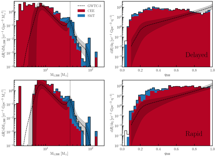
Figure 15: The primary BH mass (left) and mass ratio (right) distribution at $z=0$ of the Fryer et al. (2012) delayed (top) and rapid (bottom) remnant mass prescriptions, split into CEE and SMT formation channels. The Rapid prescription has some BHs with small primary masses, possibly due to accretion onto a NS, such that a BH is formed. $35\text{M}_{\odot}$ is marked with a dashed line.

Both prescriptions increase the number of systems around $10\text{M}_{\odot}$, bringing the predicted distribution above the observed intrinsic rate. This is most likely a result of the fact that fiducial bpass injects $10^{51}$ erg into the star, which could cause too much material to be ejected from low mass stars. However, the Delayed prescription also increases the number of systems between 2 and 5 $\text{M}_{\odot}$, while Rapid does not include these systems and has a mass gap between 3 and $5\text{M}_{\odot}$. Figure 1 shows that the Rapid and Delayed prescription are similar in the high mass regime, since both assume full fallback onto the BH. In the low mass regime, the prescriptions differ significantly from each other and from the bpass prescription. bpass generally predicts smaller remnant masses for larger CO cores than both Fryer prescriptions do, and could result in the significantly different low $\text{M}_{\text{1,BH}}$ regime. While this makes it difficult to untangle the influence from CEE, it also shows that the extended tail and excess near $35\text{M}_{\odot}$ remain with other remnant prescriptions than implemented in fiducial bpass.

6.2.2 (P)PISN

We have implemented the PPISN prescription from Farmer et al. (2019) for $\text{M}_{\text{CO}}\geq 38$, which results in a smooth transition between different remnant mass prescriptions. van Son et al. (2020) found an additional bump at $30\text{M}_{\odot}$ as a result of a non-smooth transition between the CCSN and PPISN prescription. This is not present in our remnant mass distribution. Moreover, fiducial bpass does not contain this PPISN prescription, but the $35\text{M}_{\odot}$ excess is still present.

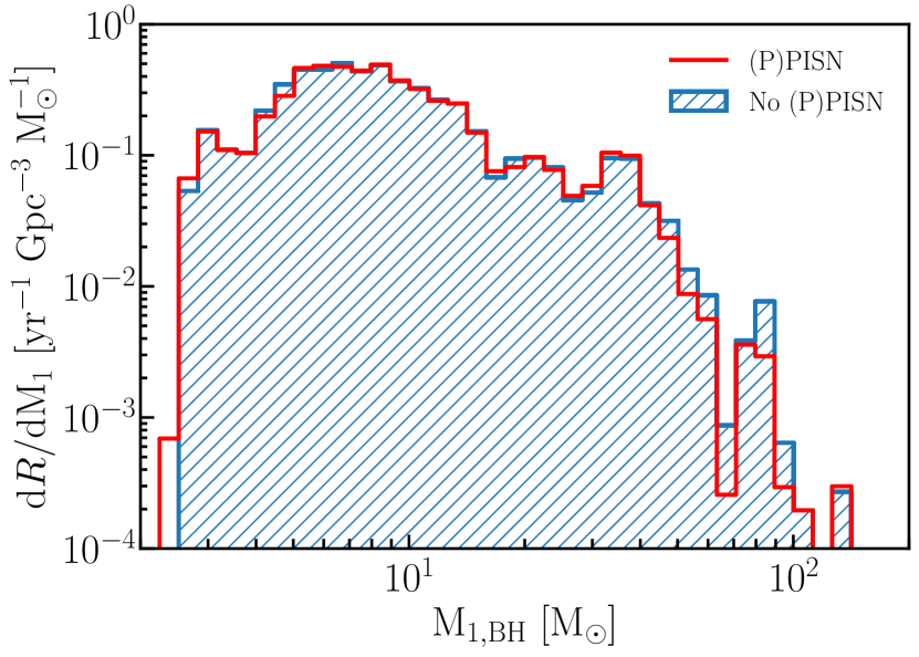
Figure 16: The $\text{M}_{\text{1,BH}}$ distribution at $z=0$ of merging BBHs for the model presented in this work with PPISN and PISN (red) and for a model without PPISN and PISN (blue). The impact of (P)PISN in bpass on the distribution is minimal.

Furthermore, in Figure 16 we have removed the PPISN and PISN prescriptions from the population synthesis and find only subtle changes in the merger rate in the PISN mass gap region. This in contrast to findings by Stevenson et al. (2019), who found that the (P)PISN influences the high-mass $\text{M}_{\text{1,BH}}$ regime. Because most of the high primary mass systems in bpass are created through accretion onto BHs with initial masses between $10-30\text{M}_{\odot}$, the impact of (P)PISN is limited in bpass, as those BHs do not come from progenitors experiencing PPISN.

7 Caveats and Uncertainties

7.1 BH spin

Besides stability of mass transfer, the efficiency of mass transfer is an important factor. To achieve high-mass BHs, we require stable mass transfer with super-Eddington accretion onto the BH. This can leave an imprint on the spin of the population, since a large amount of material is accreted from the companion. This should lead to a non-negligible spin (Zevin & Bavera, 2022) and even high spins for case A stable mass transfer (Shao & Li, 2022), albeit it is unclear if the BH remains rotating (Tchekhovskoy et al., 2012). bpass does not currently track the spin of BHs. Thus, as an alternative, we look at the amount of accreted material onto the BH, which we use as a proxy for the spin.

We find that most material is accreted by BHs in systems with $q\lesssim 0.5$, which would results in these BHs spinning with a positive spin. Furthermore, high chirp-mass systems have a lot of accreted material, as is expected, since the large chirp mass systems require material to remain in the systems. These relations are in agreement with relations for SMT systems found by Zevin et al. (2021); Zevin & Bavera (2022), and could align the observed correlation between high chirp-masses ($\mathcal{M}>40M_{\odot}$) and a positive effective spin found by (Abbott et al., 2021) under the assumption of thin disk accretion (Bardeen, 1970; King & Kolb, 1999). As such, further analysis is required to find the spin of our predicted merging BBH systems.

Another observable could be the observed BH+star binaries, which are often quickly rotating, with BH masses around $10\textrm{--}20\text{M}_{\odot}$ and have high companion masses ($31-70\text{M}_{\odot}$) (for an overview of systems, see Conclusion of Shao & Li, 2022). These systems might have been spun up during a previous mass transfer phase before a the current observed mass transfer phase. This is similar to the interactions in our models, where an initial SMT interaction takes place on the Main-Sequence, followed by a SMT or CEE interaction during a later stage of the evolution. The observed companions are often a giant or supergiant and have short periods (Miller-Jones et al., 2021; Orosz et al., 2007, 2009). Albeit depending on the metallicity and mass ratio, our models undergo SMT if the star is in this phase. However, a detailed analysis of these BH binaries is required to determine their presence in bpass and relation to the BBH merger population.

7.2 Super-Eddington Accretion

Super-Eddington accretion is required to conserve enough mass in the binary system to form massive BHs, but also to allow for more stable mass transfer due to a fast changing mass ratios. For spherically symmetric accretion, the Eddington Luminosity restricts the accretion rate onto a BH. The accretion rates onto the BH in our models are generally more than 100 times Eddington limited accretion and in rare occasions reaches $10^{4}$ times the Eddington rate. If the accretion is limited, it is uncertain whether or not the BH is still able to accrete similar amounts through longer accretion periods.

A radiation pressure dominated disk could increase the accretion rate up to 10 times Eddington (Begelman, 2002; Ruszkowski & Begelman, 2003), which can be sufficient to grow the BH. As shown by Mapelli et al. (2009) and Zampieri & Roberts (2009), marginal super-Eddington accretion could result in $30-80\text{M}_{\odot}$ BHs from low metallicity environments.

However, most bpass models accrete at a higher rate. To achieve these, other accretion methods have to occur, such as near radial inflow, neutrino emission, advection into the event horizon, or semi-relativistic polar outflows (Popham et al., 1999; Begelman, 2002; Ruszkowski & Begelman, 2003; Sądowski & Narayan, 2016; Takeo et al., 2020; Yoshioka et al., 2022). These can result in super-Eddington accretion rates between 100 and 1000 times the limit, which where most of the accretion in our models occur.

Since the super-Eddington accretion takes place on a longer than thermal timescale, these systems spend a reasonable amount of time transferring mass at a super-Eddington rate. This should make it possible to observe these systems, especially because they could emit at a super-Eddington luminosity (Klencki et al., 2022). Observationally, these could be similar to very and ultra luminous X-ray sources, like Holmberg II X-1 (Cseh et al., 2014), M101 X-1 (Liu et al., 2013; Shen et al., 2015), M83 ULX-1 (Soria et al., 2012, 2015), IC 342 X-1 (Das et al., 2021). These systems are thought to consists of a companion star and a stellar mass BH with super-Eddington accretion (Ebisawa et al., 2003; Motch et al., 2014; Ogawa et al., 2021; Wielgus et al., 2022; Ambrosi et al., 2022), although this is an area of active discussion, since it could also be an intermediate mass BH (Ramsey et al., 2006).

7.3 Mass Ratio Reversal

Super-Eddington accretion does not only leave an imprint on the spin of the systems, but also the mass ratios. Recent work from Zevin et al. (2021) has indicated that up to 72 per cent of BBH systems can undergo mass ratio reversal in optimal condition and even up to 82 per cent in populations from Broekgaarden et al. (2022). In this process, the initially more massive star become the less massive BH in the BBH merger. Observationally, mass ratio reversal is thought to be limited (Mould et al., 2022). By implementing super-Eddington accretion onto the BH, this process becomes rare and only 4 per cent of BBH systems reverse mass ratio in our population due to the material being accreted instead of blown away from the system. The mass ratio reversal that does take place in bpass is restricted to the low $\text{M}_{\text{1,BH}}$ regime with most being a result of CEE. Thus, super-Eddington accretion and more stable mass transfer leads to limited mass ratio reversal in merging BHs.

7.4 Additional Substructure in the $\text{M}_{\text{1,BH}}$ distribution

With GWTC-3, modest confidence for more substructure in the primary remnant mass distribution was found with a drop in merger rate at $14\text{M}_{\odot}$ (Abbott et al., 2021). The bpass primary BH mass distribution has a reduced number of events at $18\text{M}_{\odot}$, as is visible in Figure 8. This structure is caused by a drop in CEE systems, while the SMT channel does not increase yet. This may be caused by SMT not being able to shrink the orbit of the system sufficiently for it to merge within the Hubble time, while a CE phase is avoided by our mass transfer stability criteria. Albeit less clearly, the same substructure remains between different remnant mass prescriptions, as can be seen in Figure 15. Interestingly, in Section 6.1 this substructure becomes a plateau when QHE is limited to lower metallicities. Further investigation of this substructure will be required in the future, when the properties of the observed population are more constraint.

7.5 Other Formation Pathways

Due to approximations made in bpass models, the companion star will always be a main-sequence star before the first supernova. This limits the ability to probe interactions of double cored systems.

While we are able to predict high primary BH masses using isolated binary evolution, other formation pathways could contribute to the total BBH merger rate, such as dynamical interaction (Mapelli et al., 2021, for an overview, see). These would leave their own imprint on the population of merging BBH holes, such as random spin alignment (Zevin et al., 2021). However, due to uncertainties in other region of compact object predictions, such as the stellar physics in the isolated binary evolution, care should be taken when constraining formation pathways (Broekgaarden et al., 2021; Mandel & Broekgaarden, 2021).

In the high primary BH mass regime, hierarchical mergers have been suggested as a possibility for their formation. However, this would lead to an isotropic orientated spin distribution, which is not currently observed (Abbott et al., 2021).

8 Conclusions

We have combined bpass, a population synthesis code with detailed stellar models, with the metallicity evolution and star formation history of the TNG-100 simulation. On its own, the fiducial bpass populations can self-consistently reproduce a number of massive star evolutionary characteristics, young and old stellar populations (Wofford et al., 2016; Eldridge & Stanway, 2009; Eldridge et al., 2017; Stanway & Eldridge, 2018), and transients rates (Eldridge & Stanway, 2016; Eldridge et al., 2019; Tang et al., 2020; Ghodla et al., 2022b; Briel et al., 2022). We implement a PPISN prescription and predict the properties of the merging BBH population.

1. We find that similar to Neijssel et al. (2019) and van Son et al. (2022) that high primary BH mass mergers are a result of stable mass transfer. Moreover, our stability determination and implementation of super-Eddington accretion results in an extended primary BH mass distribution up to $100\text{M}_{\odot}$ with an excess at $35\text{M}_{\odot}$.

2. The $35\text{M}_{\odot}$ peak is not dominated by PPISN, but is a result of stable mass transfer, QHE, and stellar winds. While PPISN systems still contribute to this peak, it is not the major formation pathway for these systems. Instead, QHE limits the high-end of the peak, while unstable mass transfer limits the lower edge. In combination with the stellar winds, this results in an excess at $35\text{M}_{\odot}$, as discussed in Section 4.1.

3. The PISN mass gap BHs are a result of super-Eddington accretion in BH+star systems with $5<q<10$ (see Section 4.2). These systems are able to merge within the Hubble time due to tidal forces during Roche Lobe Overflow bringing the system together. Radial shrinkage due to mass loss and the efficient accretion by the BH, which flips the mass ratio, allows this interaction to be stable. These high-mass systems create a disconnect between the excess and the cut-off of the primary BH mass distribution, as observed.

4. Super-Eddington accretion also restricts the amount of mass ratio reversal to 4 per cent with most occurring in systems undergoing CEE (Section 7.3). Furthermore, the large amount of mass transferred onto the primary BH could leave an imprint on the spin of the BH, visible during merger. While we are currently unable to predict the spin of the system, we find that most mass is transferred in merging systems with $q\lesssim 0.5$ and high chirp masses, similar to values found by Zevin et al. (2021), aligning with observations (Section 7.1).

5. Besides the standard bpass remnant mass prescription, which injects $10^{51}$ erg into the star to determine the remnant mass, we also implement the Fryer et al. (2012) prescriptions without PPISN. Because the prescriptions are similar in the high CO core mass regime, the $35\text{M}_{\odot}$ and upper mass gap BHs remain, but the low mass regime of the $\text{M}_{\text{1,BH}}$ distribution and the mass ratio distribution changes significantly with Rapid prescription providing a closer match to the observed distributions.

6. Completely removing the PPISN and/or PISN prescription only minimally impacts the $\text{M}_{\text{1,BH}}$ distribution, because the majority of BBH progenitors in bpass do not experience PPISN or PISN.

7. Quasi-homogeneous evolution is an essential physical process in shaping the $\text{M}_{\text{1,BH}}$ distribution. Altering the QHE selection does significantly alter the $\text{M}_{\text{1,BH}}$ distribution, as discussed in Section 6.1. If high amount of mass are transferred to the companion before the first supernova, further interactions are limited due to QHE. Allowing for less QHE, the rate of the $35\text{M}_{\odot}$ excess increases and shifts it to higher masses. Implementing a detailed determination of the accretion QHE from Ghodla et al. (2022a) based on the amount of material accreted, only slightly alters the final $\text{M}_{\text{1,BH}}$ distribution.

8. Because we use detailed stellar models, we model the response of the donor star due to mass loss instead of implementing prescriptions based on the evolutionary phase of the star. We find that the stability of mass transfer depends on metallicity, mass, and age, similar to Ge et al. (2010, 2015, 2020a, 2020b). For comparison, we show the nature of the envelope for our single star models over a large range of metallicity, ZAMS masses, and ages. Most importantly, the envelope during core-helium burning is often radiative, while rapid population synthesis codes based on Hurley et al. (2002) often assume that these stars have a convective nature (for more detail, see Klencki et al., 2021). As a result, more systems undergo nuclear timescale stable mass transfer in bpass, especially at larger mass ratios between a BH and stellar companion.

While the evolution of single stars is complex and non-linear, evolution of binary stars is even more extreme. All relevant factors have to be taken into account with QHE and the stability and efficiency of mass transfer being essential in understanding the high-mass regime of the primary BH mass distribution. Besides constraining other observable properties of the population synthesis, such as (Ultra-Luminous) X-Ray binaries, future GW observations will be able to further constraint the properties of the merging BBH population and restrict the formation pathways.

Data Availability

The bpass models can be found at https://bpass.auckland.ac.nz/. The code for plots can be found on our organisational github https://github.com/UoA-Stars-And-Supernovae. The envelope and mass transfer stability data in machine readable format can be found on Github or in the Supplementary Material.

Appendix A Model uncertainties

bpass is based on a limited number of stellar models (250.000) and one concern could be the number of models contributing to the $\text{M}_{\text{1,BH}}$ distribution. To this end we calculate the number of models after the natal kick (465.047) contributing to each bin in the $\text{M}_{\text{1,BH}}$ distribution and calculate the Poisson error for each bins. The number of models after the natal kick are larger due to sampling of the natal kick distribution. The resulting Poisson errors are insignificant and, except for the lowest mass bin, are unnoticeable when added to Figure 3.

Because the ZAMS mass grid at high masses is sparse in bpass, we have selected a logarithmic binning for the $\text{M}_{\text{1,BH}}$ space to combine the systems in this regime. In Figure 17, we show the $\text{M}_{\text{1,BH}}$ distribution with linear bins of a $2\text{M}_{\odot}$ width. As can be seen the high-mass regime is sparsely populated, but the number of models contributing to each bin is still results in insignificant errors. Furthermore, the $35\text{M}_{\odot}$ excess and a substructure at $20\text{M}_{\odot}$ are still present.

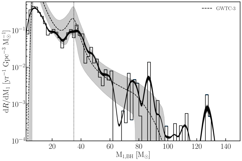
Figure 17: The $\text{M}_{\text{1,BH}}$ distribution using linear bins with a width of $2\text{M}_{\odot}$. The vertical dotted line indicates $35\text{M}_{\odot}$ and the dashed line with gray area is the GWTC-3 intrinsic population and the 95 per cent confidence interval using their pp model (Abbott et al., 2021). The thick black line are kernel density estimates from 1000 resampled populations.

Instead of binning the bpass output, we can instead apply a kernel density estimate (KDE) to the individual $\text{M}_{\text{1,BH}}$ merger samples. Using Scott’s rule for bandwidth determination, we get the solid black line in Figure 3. The KDE fluctuates significantly due to the undersampling of masses in the high-mass regime and small event rates. The $35\text{M}_{\odot}$ peak wider and peaks slightly higher and the substructure at $20\text{M}_{\odot}$ is clearly visible. This indicates that both these features are part of distribution and not a binning artefact. Furthermore, we perform 1000 resamplings of the data by redrawing the same number of models as the original $\text{M}_{\text{1,BH}}$ distribution with each model weighted equally. We run the new populations through the KDE, which show as the thick solid black line in Figure 17. Although some statistical uncertainty is present, it does not significantly impact the $\text{M}_{\text{1,BH}}$ distribution or its features.

The features in the $\text{M}_{\text{1,BH}}$ distribution remain when changing bins and when applying a kernel density estimation. While the high $\text{M}_{\text{1,BH}}$ range is undersampled, sufficient models contribute to each mass for the statistical error to be negligible. Of course, this does not take into account uncertainty based on the implemented physics.

Appendix B Homology

In the context of mass transfer the thermal timescale of the star are important because it limits the accretion onto the companion star. Within bpass this limit is $\dot{\mathrm{M}}=\mathrm{M}_{2}/\tau_{\mathrm{KH}}$. Thus, the timescale at which the primary loses the mass and at which the secondary star can accrete this material determines the mass lost from the system. To be able to get massive BHs, it is essential that material remains in the system and that the timescales are similar. To understand the behaviour of the stellar models, we use homology relations to determine the dependence of the thermal timescale on mass between different stars (Found in most stellar structure text books, such as Eldridge & Tout, 2019). The thermal timescale is proportional to the mass, luminosity and radius of the star, as per Equation 5.

$$\tau_{\text{KH}}\propto\frac{M^{2}}{RL}$$ (5)

To determine the dependence solely on mass, we setup a few basic scaling relations that approximate the behaviour of massive stars before turning our attention to specific regimes. From the first two stellar structure equations, we get the following main homology relations in which $\rho_{c}$ and $P_{c}$ are the central temperatures of the star with mass $M$ and radius $R$.

$$\rho_{c}\propto\frac{M}{R^{3}}$$ (6)

$$P_{c}\propto\frac{M^{2}}{R^{4}}$$ (7)

We use the stelar structure equation of radiative energy transport and electron scattering ($\kappa\propto 1+X$) for the star. After applying Equation 6, we get Equation 8.

$$\frac{T_{c}}{R}\propto\frac{\kappa\rho_{c}L}{R^{2}T_{c}^{3}}\longrightarrow L\propto T_{c}^{4}\frac{R^{4}}{M}\frac{1}{1+X},$$ (8)

where $T_{c}$ is the central temperature, $L$ the luminosity of the star, and $X$ the hydrogen fraction.

Finally, we use the energy generation of the star to get Equation 9. Since the main energy generation for massive stars is through the CNO-cycle, we have $\nu\approx 18$.

$$\frac{L}{R}\propto R^{2}\rho_{c}^{2}T_{c}^{\nu}\longrightarrow L\propto\frac{M^{2}}{R^{3}}T_{c}^{18}$$ (9)

B.1 Gas pressure dominated

At the low end of massive stars, the star is dominated by gas pressure and the equation of state follows the ideal gas law, where $\mu$ is the mean molecular weight in the star.

$$P_{c}\propto\frac{\rho_{c}T_{c}}{\mu}\longrightarrow T_{c}\propto\mu\frac{M}{R}$$ (10)

This allows us to transform Equations 8 into

$$L\propto\frac{\mu^{4}}{1+X}M^{3}$$ (11)

And combine it with 9 to get:

$$L\propto\mu^{18}\frac{M^{20}}{R^{21}}\longrightarrow\frac{\mu^{4}}{1+X}M^{3}\propto\mu^{18}\frac{M^{20}}{R^{21}}$$ (12)

Eventually, we get the relation between radius and mass.

$$R\propto\mu^{18/21}(1+X)M^{17/21}$$ (13)

Combining Equations 11, 12, 13 with Equation 5, we find that for the ideal gas equation of state, the thermal timescale scales as follows:

$$\tau_{\text{KH}}\propto\frac{M^{2}}{M^{17/21}M^{3}}\propto M^{-38/21}\propto M^{-1.81}$$ (14)

B.2 Radiation pressure dominated

At higher masses, radiation pressure plays an essential role in supporting the star. Thus, the ideal gas equation of state is no longer valid. While the actual dynamics will be a combination of radiation and gas pressure, we can look at the extreme example with only radiation pressure. Instead of Equation 10, we get the following relation for the central temperature

$$P_{c}\propto T^{4}_{c}\longrightarrow T^{4}_{c}\propto\frac{M^{2}}{R^{4}}$$ (15)

This gives us the following equations for the luminosity and radius.

$$L\propto\frac{1}{1+X}M$$ (16)

$$L\propto\frac{M^{10}}{R^{21}}\longrightarrow\frac{M}{1+X}\propto\frac{M^{10}}{R^{21}}\longrightarrow R\propto M^{10/21}$$ (17)

Using them we find the relation between the thermal timescale and mass in radiation pressure only regime.

$$\tau_{\text{KH}}\propto M^{11/21}\propto M^{0.52}$$ (18)

B.3 Relations within the bpass models

The previous two sections cover two extreme cases. In reality, both the gas and radiation pressure contribute to the total internal pressure in the star. However, the difference in thermal timescale dependence on the mass is significant and means that at higher masses, where radiation pressure dominates, the thermal timescale becomes constant with mass.

To verify this, we plot the thermal timescale at ZAMS of all bpass single star models in Figure 18. At sub-solar metallicity, where BBH mergers are though to originate from (Belczynski et al., 2010; Stevenson et al., 2017, 2019; Santoliquido et al., 2021), the thermal timescale becomes close to constant for high masses. Thus, if mass is lost on a thermal timescale, most of it can be accreted by the companion, because the timescales are similar.

At higher metallicities, the timescales no longer become constant, which is most likely due to the change in the opacity of the star.

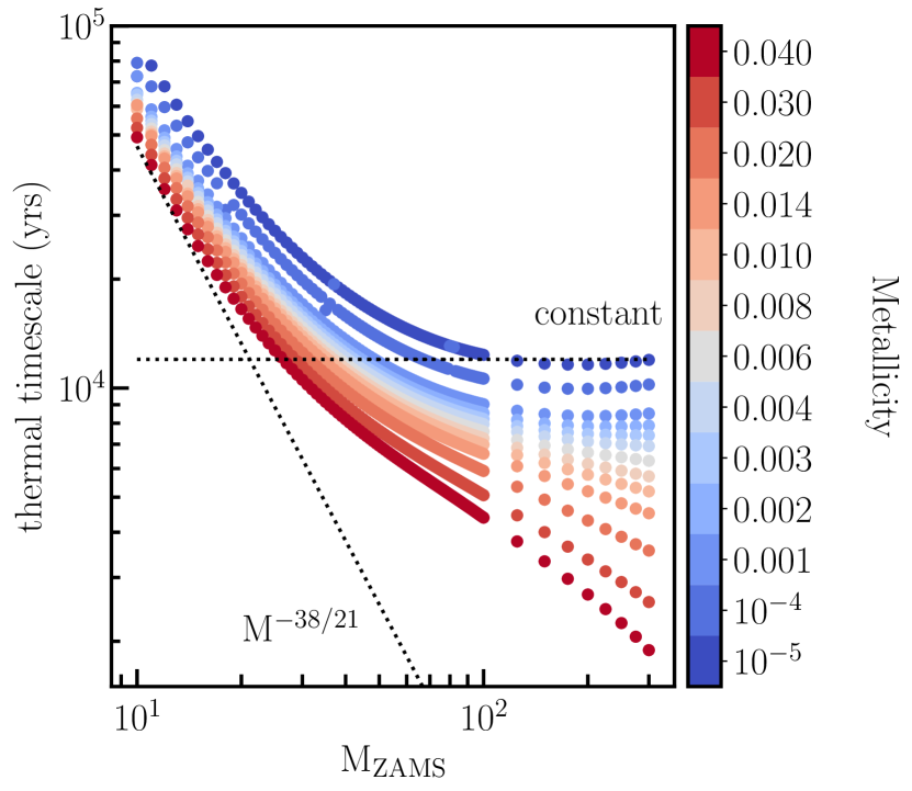
Figure 18: The thermal timescale at ZAMS of all bpass single star model per metallicity. The dashed lines indicate a $\tau_{\text{KH}}\propto M^{-38/21}$ relation and the thermal timescale being constant.

References

- Abbott et al. (2021) Abbott R., Collaboration T. L. S., Collaboration T. V., Collaboration T. K. S., 2021, ArXiv211103634 Astro-Ph Physicsgr-Qc
- Aghanim et al. (2020) Aghanim N., et al., 2020, A&A, 641, A6
- Ambrosi et al. (2022) Ambrosi E., Zampieri L., Pintore F., Wolter A., 2022, Mon. Not. R. Astron. Soc., 509, 4694
- Arca-Sedda et al. (2020) Arca-Sedda M., Mapelli M., Spera M., Benacquista M., Giacobbo N., 2020, Astrophys. J., 894, 133
- Arca-Sedda et al. (2021) Arca-Sedda M., Mapelli M., Benacquista M., Spera M., 2021, ArXiv210912119 Astro-Ph Physicsgr-Qc
- Ballone et al. (2022) Ballone A., Costa G., Mapelli M., MacLeod M., 2022, Formation of Black Holes in the Pair-Instability Mass Gap: Hydrodynamical Simulation of a Head-on Massive Star Collision
- Banerjee (2022) Banerjee S., 2022, Binary Black Hole Mergers from Young Massive Clusters in the Pair-Instability Supernova Mass Gap (arXiv:2109.14612), doi:10.48550/arXiv.2109.14612
- Bardeen (1970) Bardeen J. M., 1970, Nature, 226, 64
- Bavera et al. (2021) Bavera S. S., et al., 2021, Astron. Astrophys., 647, A153
- Begelman (2002) Begelman M. C., 2002, ApJ, 568, L97
- Belczynski et al. (2010) Belczynski K., Dominik M., Bulik T., O’Shaughnessy R., Fryer C., Holz D. E., 2010, Astrophys. J., 715, L138
- Belczynski et al. (2016) Belczynski K., Repetto S., Holz D. E., O’Shaughnessy R., Bulik T., Berti E., Fryer C., Dominik M., 2016, ApJ, 819, 108
- Belczynski et al. (2020) Belczynski K., et al., 2020, A&A, 636, A104
- Bouffanais et al. (2021) Bouffanais Y., Mapelli M., Santoliquido F., Giacobbo N., Di Carlo U. N., Rastello S., Artale M. C., Iorio G., 2021, ArXiv210212495 Astro-Ph
- Breivik et al. (2020) Breivik K., et al., 2020, Astrophys. J., 898, 71
- Briel et al. (2022) Briel M. M., Eldridge J. J., Stanway E. R., Stevance H. F., Chrimes A. A., 2022, Mon. Not. R. Astron. Soc.
- Broekgaarden et al. (2021) Broekgaarden F. S., et al., 2021, Impact of Massive Binary Star and Cosmic Evolution on Gravitational Wave Observations II: Double Compact Object Rates and Properties
- Broekgaarden et al. (2022) Broekgaarden F. S., Stevenson S., Thrane E., 2022, Signatures of Mass Ratio Reversal in Gravitational Waves from Merging Binary Black Holes (arXiv:2205.01693)
- Cameron & Mock (1967) Cameron A. G. W., Mock M., 1967, Nature, 215, 464
- Chamel et al. (2013) Chamel N., Haensel P., Zdunik J. L., Fantina A. F., 2013, Int. J. Mod. Phys. E, 22, 1330018
- Chruslinska & Nelemans (2019) Chruslinska M., Nelemans G., 2019, Mon. Not. R. Astron. Soc., 488, 5300
- Chruslinska et al. (2019) Chruslinska M., Nelemans G., Belczynski K., 2019, Mon. Not. R. Astron. Soc., 482, 5012
- Costa et al. (2022) Costa G., Ballone A., Mapelli M., Bressan A., 2022, Mon. Not. R. Astron. Soc.
- Cseh et al. (2014) Cseh D., et al., 2014, Monthly Notices of the Royal Astronomical Society: Letters, 439, L1
- Darwin (1879) Darwin G. H., 1879, Proc. R. Soc. Lond., 29, 168
- Das et al. (2021) Das S., Nandi A., Agrawal V. K., Dihingia I. K., Majumder S., 2021, Mon. Not. R. Astron. Soc., 507, 2777
- De et al. (2020) De S., MacLeod M., Everson R. W., Antoni A., Mandel I., Ramirez-Ruiz E., 2020, Astrophys. J., 897, 130
- Di Carlo et al. (2020) Di Carlo U. N., et al., 2020, Mon. Not. R. Astron. Soc., 498, 495
- Dominik et al. (2012) Dominik M., Belczynski K., Fryer C., Holz D. E., Berti E., Bulik T., Mandel I., O’Shaughnessy R., 2012, ApJ, 759, 52
- Dorozsmai & Toonen (2022) Dorozsmai A., Toonen S., 2022, Importance of Stable Mass Transfer and Stellar Winds for the Formation of Gravitational Wave Sources (arXiv:2207.08837), doi:10.48550/arXiv.2207.08837
- Ebisawa et al. (2003) Ebisawa K., Życki P., Kubota A., Mizuno T., Watarai K.-y., 2003, ApJ, 597, 780
- Eggleton (1971) Eggleton P. P., 1971, Monthly Notices of the Royal Astronomical Society, 151, 351
- Eggleton (2011) Eggleton P., 2011, Evolutionary Processes in Binary and Multiple Stars
- Eldridge & Stanway (2009) Eldridge J. J., Stanway E. R., 2009, Monthly Notices of the Royal Astronomical Society, 400, 1019
- Eldridge & Stanway (2016) Eldridge J. J., Stanway E. R., 2016, Mon. Not. R. Astron. Soc., 3313, 3302
- Eldridge & Tout (2004) Eldridge J. J., Tout C. A., 2004, Mon. Not. R. Astron. Soc., 353, 87
- Eldridge & Tout (2019) Eldridge J. J., Tout C. A., 2019, The Structure and Evolution of Stars. World Scientific Publishing Co. Pte. Ltd, doi:10.1142/p974
- Eldridge et al. (2008) Eldridge J. J., Izzard R. G., Tout C. A., 2008, Mon. Not. R. Astron. Soc., 384, 1109
- Eldridge et al. (2017) Eldridge J. J., Stanway E. R., Xiao L., McClelland L. A. S., Taylor G., Ng M., Greis S. M. L., Bray J. C., 2017, Publ. Astron. Soc. Aust., 34, e058
- Eldridge et al. (2019) Eldridge J. J., Stanway E. R., Tang P. N., 2019, Mon. Not. R. Astron. Soc., 482, 870
- Farag et al. (2022) Farag E., Renzo M., Farmer R., Chidester M. T., Timmes F. X., 2022, Resolving The Peak Of The Black Hole Mass Spectrum
- Farmer et al. (2019) Farmer R., Renzo M., de Mink S. E., Marchant P., Justham S., 2019, Astrophys. J., 887, 53
- Fowler & Hoyle (1964) Fowler W. A., Hoyle F., 1964, ApJS, 9, 201
- Fryer et al. (2012) Fryer C. L., Belczynski K., Wiktorowicz G., Dominik M., Kalogera V., Holz D. E., 2012, ApJ, 749, 91
- Gallegos-Garcia et al. (2021) Gallegos-Garcia M., Berry C. P. L., Marchant P., Kalogera V., 2021, Astrophys. J., 922, 110
- Ge et al. (2010) Ge H., Hjellming M. S., Webbink R. F., Chen X., Han Z., 2010, Astrophys. J., 717, 724
- Ge et al. (2015) Ge H., Webbink R. F., Chen X., Han Z., 2015, Astrophys. J., 812, 40
- Ge et al. (2020a) Ge H., Webbink R. F., Han Z., 2020a, Astrophys. J. Suppl. Ser., 249, 9
- Ge et al. (2020b) Ge H., Webbink R. F., Chen X., Han Z., 2020b, Astrophys. J., 899, 132
- Ghodla et al. (2022a) Ghodla S., Eldridge J. J., Stanway E. R., Stevance H. F., 2022a, Evaluating Accretion & Tidally Induced Chemically Homogeneous Evolution in Stellar Binaries: Electromagnetic Implications
- Ghodla et al. (2022b) Ghodla S., van Zeist W. G. J., Eldridge J. J., Stevance H. F., Stanway E. R., 2022b, Mon. Not. R. Astron. Soc., 511, 1201
- Giacobbo et al. (2018) Giacobbo N., Mapelli M., Spera M., 2018, Monthly Notices of the Royal Astronomical Society, 474, 2959
- Harris et al. (2020) Harris C. R., et al., 2020, Nature, 585, 357
- Heger & Woosley (2002) Heger A., Woosley S. E., 2002, ApJ, 567, 532
- Hjellming & Webbink (1987) Hjellming M. S., Webbink R. F., 1987, Astrophys. J., 318, 794
- Hobbs et al. (2005) Hobbs G., Lorimer D. R., Lyne A. G., Kramer M., 2005, Mon. Not. R. Astron. Soc., 360, 974
- Hunter (2007) Hunter J. D., 2007, Comput. Sci. Eng., 9, 90
- Hurley et al. (2002) Hurley J. R., Tout C. A., Pols O. R., 2002, Mon. Not. R. Astron. Soc., 329, 897
- Iben & Livio (1993) Iben I. J., Livio M., 1993, Publ. Astron. Soc. Pac., 105, 1373
- Ivanova et al. (2013) Ivanova N., et al., 2013, Astron. Astrophys. Rev., 21, 59
- King & Kolb (1999) King A. R., Kolb U., 1999, Monthly Notices of the Royal Astronomical Society, 305, 654
- Klencki et al. (2020) Klencki J., Nelemans G., Istrate A. G., Pols O., 2020, A&A, 638, A55
- Klencki et al. (2021) Klencki J., Nelemans G., Istrate A. G., Chruslinska M., 2021, Astron. Astrophys., 645, 27
- Klencki et al. (2022) Klencki J., Istrate A., Nelemans G., Pols O., 2022, Astron. Amp Astrophys. Vol. 662 IdA56 NUMPAGES24NUMPAGES Pp, 662, A56
- Kroupa (2001) Kroupa P., 2001, MNRAS, 322, 231
- Langer & Norman (2006) Langer N., Norman C. A., 2006, The Astrophysical Journal Letters, 638, L63
- Laplace et al. (2021) Laplace E., Justham S., Renzo M., Götberg Y., Farmer R., Vartanyan D., de Mink S. E., 2021, Astron. Amp Astrophys. Vol. 656 IdA58 NUMPAGES29NUMPAGES Pp, 656, A58
- Liu et al. (2013) Liu J.-F., Bregman J. N., Bai Y., Justham S., Crowther P., 2013, Nature, 503, 500
- Madau & Dickinson (2014) Madau P., Dickinson M., 2014, Annu. Rev. Astron. Astrophys., 52, 415
- Mandel & Broekgaarden (2021) Mandel I., Broekgaarden F. S., 2021, Rates of Compact Object Coalescences
- Mandel et al. (2020) Mandel I., Mueller B., Riley J., de Mink S. E., Vigna-Gomez A., Chattopadhyay D., 2020, Mon. Not. R. Astron. Soc., 500, 1380
- Mapelli et al. (2009) Mapelli M., Colpi M., Zampieri L., 2009, Mon. Not. R. Astron. Soc., 395, L71
- Mapelli et al. (2021) Mapelli M., et al., 2021, ArXiv210305016 Astro-Ph
- Marchant & Moriya (2020) Marchant P., Moriya T. J., 2020, Astron. Amp Astrophys. Vol. 640 IdL18 NUMPAGES8NUMPAGES Pp, 640, L18
- Marchant et al. (2019) Marchant P., Renzo M., Farmer R., Pappas K. M. W., Taam R. E., de Mink S. E., Kalogera V., 2019, Astrophys. J., 882, 36
- Marchant et al. (2021) Marchant P., Pappas K. M. W., Gallegos-Garcia M., Berry C. P. L., Taam R. E., Kalogera V., Podsiadlowski P., 2021, Astron. Astrophys., 650, A107
- Marinacci et al. (2018) Marinacci F., et al., 2018, Mon. Not. R. Astron. Soc., 480, 5113
- Mehta et al. (2022) Mehta A. K., Buonanno A., Gair J., Miller M. C., Farag E., deBoer R. J., Wiescher M., Timmes F. X., 2022, Astrophys. J., 924, 39
- Miller-Jones et al. (2021) Miller-Jones J. C. A., et al., 2021, Science, 371, 1046
- Moe & Di Stefano (2017) Moe M., Di Stefano R., 2017, ApJS, 230, 15
- Motch et al. (2014) Motch C., Pakull M. W., Soria R., Grisé F., Pietrzyński G., 2014, Nature, 514, 198
- Mould et al. (2022) Mould M., Gerosa D., Broekgaarden F. S., Steinle N., 2022, Which Black Hole Formed First? Mass-ratio Reversal in Massive Binary Stars from Gravitational-Wave Data (arXiv:2205.12329), doi:10.48550/arXiv.2205.12329
- Naiman et al. (2018) Naiman J. P., et al., 2018, Mon. Not. R. Astron. Soc., 477, 1206
- Neijssel et al. (2019) Neijssel C. J., et al., 2019, Monthly Notices of the Royal Astronomical Society, 490, 3740
- Nelemans & Tout (2005) Nelemans G., Tout C. A., 2005, Mon. Not. R. Astron. Soc., 356, 753
- Nelemans et al. (2000) Nelemans G., Verbunt F., Yungelson L. R., Portegies Zwart S. F., 2000, Astron. Astrophys., 360, 1011
- Nelson et al. (2018) Nelson D., et al., 2018, Mon. Not. R. Astron. Soc., 475, 624
- Nugis & Lamers (2000) Nugis T., Lamers H. J. G. L. M., 2000, Astron. Astrophys., 360, 227
- Ogawa et al. (2021) Ogawa T., Ohsuga K., Makino Y., Mineshige S., 2021, Publications of the Astronomical Society of Japan, 73, 701
- Olejak & Belczynski (2021) Olejak A., Belczynski K., 2021, ApJL, 921, L2
- Olejak et al. (2021) Olejak A., Belczynski K., Ivanova N., 2021, Astron. Astrophys., 651, 17
- Orosz et al. (2007) Orosz J. A., et al., 2007, Nature, 449, 872
- Orosz et al. (2009) Orosz J. A., et al., 2009, ApJ, 697, 573
- Paczynski (1976) Paczynski B., 1976, in Structure and Evolution of Close Binary Systems. D. Reidel Publishing Co., Cambridge, England, p. 75
- Passy et al. (2012) Passy J.-C., Herwig F., Paxton B., 2012, Astrophys. J., 760, 90
- Pavlovskii & Ivanova (2015) Pavlovskii K., Ivanova N., 2015, Mon. Not. R. Astron. Soc., 449, 4415
- Pavlovskii et al. (2017) Pavlovskii K., Ivanova N., Belczynski K., Van K. X., 2017, Mon. Not. R. Astron. Soc., 465, 2092
- Paxton et al. (2011) Paxton B., Bildsten L., Dotter A., Herwig F., Lesaffre P., Timmes F., 2011, Astrophys. J. Suppl. Ser., 192, 3
- Paxton et al. (2013) Paxton B., et al., 2013, Astrophys. J. Suppl. Ser., 208, 4
- Paxton et al. (2015) Paxton B., et al., 2015, Astrophys. J. Suppl. Ser., 220, 15
- Paxton et al. (2018) Paxton B., et al., 2018, Astrophys. J. Suppl. Ser., 234, 34
- Paxton et al. (2019) Paxton B., et al., 2019, Astrophys. J. Suppl. Ser., 243, 10
- Peters (1964) Peters P. C., 1964, Phys. Rev., 136, B1224
- Pillepich et al. (2018) Pillepich A., et al., 2018, Mon. Not. R. Astron. Soc., 475, 648
- Podsiadlowski (2001) Podsiadlowski P., 2001, in Evolution of Binary and Multiple Star Systems; A Meeting in Celebration of Peter Eggleton’s 60th Birthday.. p. 239
- Popham et al. (1999) Popham R., Woosley S. E., Fryer C., 1999, Astrophys. J., 518, 356
- Rakavy & Shaviv (1967) Rakavy G., Shaviv G., 1967, The Astrophysical Journal, 148, 803
- Ramsey et al. (2006) Ramsey C. J., Williams R. M., Gruendl R. A., Chen C. H. R., Chu Y.-H., Wang Q. D., 2006, Astrophys. J., 641, 241
- Reback et al. (2020) Reback J., et al., 2020, Pandas-Dev/Pandas: Pandas 1.0.3, Zenodo, doi:10.5281/zenodo.3715232
- Renzo & Zapartas (2020) Renzo M., Zapartas E., 2020, Contrib. Astron. Obs. Skaln. Pleso, 50, 472
- Renzo et al. (2020a) Renzo M., Farmer R. J., Justham S., de Mink S. E., Götberg Y., Marchant P., 2020a, Monthly Notices of the Royal Astronomical Society, 493, 4333
- Renzo et al. (2020b) Renzo M., Cantiello M., Metzger B. D., Jiang Y. F., 2020b, Astrophys. J., 904, L13
- Riley et al. (2022) Riley J., et al., 2022, Astrophys. J. Suppl. Ser., 258, 34
- Rodriguez et al. (2019) Rodriguez C. L., Zevin M., Amaro-Seoane P., Chatterjee S., Kremer K., Rasio F. A., Ye C. S., 2019, Phys. Rev. D, 100, 043027
- Ruszkowski & Begelman (2003) Ruszkowski M., Begelman M. C., 2003, ApJ, 586, 384
- Sądowski & Narayan (2016) Sądowski A., Narayan R., 2016, Mon. Not. R. Astron. Soc., 456, 3929
- Sana et al. (2012) Sana H., et al., 2012, Science, 337, 444
- Sana et al. (2013) Sana H., et al., 2013, Astron. Amp Astrophys. Vol. 550 IdA107 NUMPAGES22NUMPAGES Pp, 550, A107
- Santoliquido et al. (2020) Santoliquido F., Mapelli M., Bouffanais Y., Giacobbo N., Di Carlo U. N., Rastello S., Artale M. C., Ballone A., 2020, Astrophys. J., 898, 152
- Santoliquido et al. (2021) Santoliquido F., Mapelli M., Giacobbo N., Bouffanais Y., Artale M. C., 2021, Mon. Not. R. Astron. Soc., 502, 4877
- Shao & Li (2021) Shao Y., Li X.-D., 2021, Astrophys. J., 920, 81
- Shao & Li (2022) Shao Y., Li X.-D., 2022, Astrophys. J., 930, 26
- Shen et al. (2015) Shen R.-F., Duran R. B., Nakar E., Piran T., 2015, Mon. Not. R. Astron. Soc. Lett., 447, L60
- Soberman et al. (1997) Soberman G. E., Phinney E. S., van den Heuvel E. P. J., 1997, Astron. Astrophys., pp 620–635
- Soria et al. (2012) Soria R., Kuntz K. D., Winkler P. F., Blair W. P., Long K. S., Plucinsky P. P., Whitmore B. C., 2012, ApJ, 750, 152
- Soria et al. (2015) Soria R., Kuntz K. D., Long K. S., Blair W. P., Plucinsky P. P., Winkler P. F., 2015, ApJ, 799, 140
- Spera & Mapelli (2017) Spera M., Mapelli M., 2017, Monthly Notices of the Royal Astronomical Society, 470, 4739
- Springel et al. (2018) Springel V., et al., 2018, Mon. Not. R. Astron. Soc., 475, 676
- Stanway & Eldridge (2018) Stanway E. R., Eldridge J. J., 2018, Mon. Not. R. Astron. Soc., 479, 75
- Stanway et al. (2018) Stanway E. R., Hoskin M. J., Lane M. A., Brown G. C., Childs H. J., Greis S. M., Levan A. J., 2018, Mon. Not. R. Astron. Soc., 475, 1829
- Stȩpień (2011) Stȩpień K., 2011, Astron. Amp Astrophys. Vol. 531 IdA18 NUMPAGES4NUMPAGES Pp, 531, A18
- Stevenson et al. (2017) Stevenson S., Vigna-Gómez A., Mandel I., Barrett J. W., Neijssel C. J., Perkins D., de Mink S. E., 2017, Nat. Commun., 8, 14906
- Stevenson et al. (2019) Stevenson S., Sampson M., Powell J., Vigna-Gómez A., Neijssel C. J., Szécsi D., Mandel I., 2019, Astrophys. J., 882, 121
- Takeo et al. (2020) Takeo E., Inayoshi K., Mineshige S., 2020, Mon. Not. R. Astron. Soc., 497, 302
- Tang et al. (2020) Tang P. N., Eldridge J. J., Stanway E. R., Bray J. C., 2020, Mon. Not. R. Astron. Soc. Lett., 493, L6
- Tchekhovskoy et al. (2012) Tchekhovskoy A., McKinney J. C., Narayan R., 2012, J. Phys.: Conf. Ser., 372, 012040
- Vink et al. (2001) Vink J. S., de Koter A., Lamers H. J. G. L. M., 2001, Astron. Astrophys., 369, 574
- Webbink (1984) Webbink R. F., 1984, The Astrophysical Journal, 277, 355
- Wielgus et al. (2022) Wielgus M., et al., 2022, Mon. Not. R. Astron. Soc., 514, 780
- Wiktorowicz et al. (2015) Wiktorowicz G., Sobolewska M., Sądowski A., Belczynski K., 2015, Astrophys. J., 810, 20
- Wofford et al. (2016) Wofford A., et al., 2016, Mon. Not. R. Astron. Soc., 457, 4296
- Woods & Ivanova (2011) Woods T. E., Ivanova N., 2011, Astrophys. J., 739, L48
- Woosley (2017) Woosley S. E., 2017, ApJ, 836, 244
- Woosley & Heger (2021) Woosley S. E., Heger A., 2021, Astrophys. J., 912, L31
- Woosley et al. (2002) Woosley S. E., Heger A., Weaver T. A., 2002, Rev. Mod. Phys., 74, 1015
- Yang et al. (2019) Yang Y., et al., 2019, Phys. Rev. Lett., 123, 181101
- Yoshioka et al. (2022) Yoshioka S., Mineshige S., Ohsuga K., Kawashima T., Kitaki T., 2022, Large-Scale Outflow Structure and Radiation Properties of Super-Eddington Flow: Dependence on the Accretion Rates
- Zampieri & Roberts (2009) Zampieri L., Roberts T. P., 2009, Mon. Not. R. Astron. Soc., 400, 677
- Zevin & Bavera (2022) Zevin M., Bavera S. S., 2022, ArXiv220302515 Astro-Ph Physicsgr-Qc
- Zevin et al. (2021) Zevin M., et al., 2021, ApJ, 910, 152
- de Jager et al. (1988) de Jager C., Nieuwenhuijzen H., van der Hucht K. A., 1988, Astron. Astrophys. Suppl. Ser. ISSN 0365-0138, 72, 259
- van Son et al. (2020) van Son L. A. C., et al., 2020, Astrophys. J., 897, 100
- van Son et al. (2022) van Son L. A. C., et al., 2022, Astrophys. J., 931, 17