Chemical Evolution of R-process Elements in Stars (CERES)

Abstract

Aims. The Chemical Evolution of R-process Elements in Stars (CERES) project aims to provide a homogeneous analysis of a sample of metal-poor stars ([Fe/H]¡–1.5). We present the stellar parameters and the chemical abundances of elements up to Zr for a sample of 52 giant stars.

Methods. We relied on a sample of high signal-to-noise UVES spectra. We determined stellar parameters from Gaia photometry and parallaxes. Chemical abundances were derived using spectrum synthesis and model atmospheres.

Results. We determined chemical abundances of 26 species of 18 elements: Na, Mg, Al, Si, Ca, Sc, Ti, V, Cr, Mn, Fe, Co, Ni, Cu, Zn, Sr, Y, and Zr. For several stars, we were able to measure both neutral and ionised species, including Si, Sc, Mn, and Zr. We have roughly doubled the number of measurements of Cu for stars at [Fe/H] $\leq-2.5$. The homogeneity of the sample made it possible to highlight the presence of two Zn-rich stars ([Zn/Fe]$\sim$+0.7), one r-rich and the other r-poor. We report the existence of two branches in the [Zn/Fe] versus [Ni/Fe] plane and suggest that the high [Zn/Fe] branch is the result of hypernova nucleosynthesis. We discovered two stars with peculiar light neutron-capture abundance patterns: CES1237+1922 (also known as BS 16085-0050), which is $\sim$1 dex underabundant in Sr, Y, and Zr with respect to the other stars in the sample, and CES2250-4057 (also known as HE 2247-4113), which shows a $\sim$1 dex overabundance of Sr with respect to Y and Zr.

Conclusions. The high quality of our dataset allowed us to measure hardly detectable ions. This can provide guidance in the development of line formation computations that take deviations from local thermodynamic equilibrium and hydrodynamical effects into account.

1 Introduction

The elements beyond the Fe-peak, that is, all elements with atomic number $Z>30$, are commonly referred to as ‘heavy elements’ or ‘neutron-capture’ (n-capture) elements, as the most efficient way to form these elements is through neutron captures. A neutron capture tends to create a nucleus that is away from the nuclear stability valley, and the system tries to fall back to the valley through $\beta$ decay.

From a theoretical point of view, three neutron-capture processes can be distinguished, depending on the neutron flux. When the seed nucleus has time to $\beta$ decay after each neutron capture, one refers to this as the slow neutron-capture process ($s$ process), which occurs at neutron densities of less than about $10^{8}$ cm^-3 (e.g. Busso et al., 1999, and references therein). The rapid neutron-capture process ($r$ process) occurs when the neutron flux is so high that a seed nucleus can capture several neutrons before decaying. The $r$ process requires neutron densities in excess of $10^{24}$ cm^-3 (e.g. Kratz et al., 2007, and references therein). In the intermediate neutron density regime ($10^{14}\rm\,cm^{-3}\leq N_{n}\leq 10^{16}\,cm^{-3}$) one talks about the intermediate neutron-capture process ($i$ process; Cowan & Rose, 1977). Sometimes in the literature, Zn ($Z=30$) is not considered part of this set of elements since it may also be formed through different nucleosynthetic channels, but neutron captures are definitely a possibility for synthesising Zn (Bisterzo et al., 2004). The same is true for Cu, but we consider Cu to be part of the iron-peak elements.

Observationally, it has been known for many years that, in metal-poor stars, the abundance ratios [X/Fe], where X is an n-capture element, show a large scatter as a function of [Fe/H] (McWilliam et al., 1995; Burris et al., 2000; François et al., 2007; Hansen et al., 2012), at variance with the lighter elements, for example Mg, which show a very tight relation with [Fe/H] (McWilliam et al., 1995; Cayrel et al., 2004; Bonifacio et al., 2009). This has generally been interpreted as evidence that the production of n-capture elements occurs in different sites and under different physical conditions, in contrast to the lighter elements that are formed in either hydrostatic or explosive burning in Type II or Type Ia supernovae (SNe) (see e.g. Arnett, 1996).

Based on then-existing observations and theoretical considerations, Truran (1981) argued that in metal-poor stars the n-capture elements can only be formed through the $r$ process, essentially because the only then-recognised source of $s-$process nucleosynthesis, asymptotic giant branch stars, would not have had enough time to enrich the interstellar medium before the metallicity rose above $\rm[Fe/H]=-1.5$. This is sometimes referred to as the $r-$only paradigm. It is currently believed that fast rotating massive stars can produce $s-$process elements and deliver them through their winds, prior to the SN explosion (Prantzos et al., 1990; Pignatari et al., 2010; Choplin et al., 2018; Banerjee et al., 2018; Skúladóttir et al., 2020). Although the site of the $i$ process has not yet been robustly identified, it is considered for the production of some isotopes (Hampel et al., 2016; Côté et al., 2018; Denissenkov et al., 2019; Koch et al., 2019; Skúladóttir et al., 2020; Choplin et al., 2021). More exotic phenomena, such as proton ingestion phenomena, are also believed to be responsible for the production of some n-capture elements (Hollowell et al., 1990; Fujimoto et al., 2000; Cristallo et al., 2009; Caffau et al., 2019). Even if Truran’s intuition is probably correct and the majority of n-capture elements at low metallicities are formed by the $r$ process, other processes cannot be ignored and may, in fact, contribute to the large scatter observed in the abundance ratios of these elements and to the variety of abundance patterns. Furthermore, it is now accepted that the $r$ process is not universal, but can occur in different astrophysical sites under different physical conditions, of which at least two are necessary to explain the observations (Qian & Wasserburg, 2001, 2007; Hansen et al., 2014b; Spite et al., 2018; Skúladóttir & Salvadori, 2020).

The Chemical Evolution of R-process Elements in Stars (CERES) project has the objective of characterising the abundances of as many n-capture elements as possible in a sample of giant stars of low metallicity ([Fe/H]$<-1.5$). The aim of CERES is to provide a high quality set of abundances that can be used to test different theoretical scenarios. To achieve this, we rely on a set of high resolution and high signal-to-noise ratio (S/N) spectra, and on the photometry and parallaxes provided by the Gaia satellite (Gaia Collaboration et al., 2016) to analyse all the stars in a homogeneous way. In this first paper of the series, we provide the atmospheric parameters and abundances of 18 elements, Na, Mg, Al, Si, Ca, Sc, Ti, V, Cr, Mn, Fe, Co, Ni, Cu, Zn, Sr, Y, and Zr, the last three of which are n-capture elements. Abundances of other n-capture elements shall be provided in subsequent papers of the series, based on the same atmospheric parameters.

The current paper is organised as follows: Sect. 2 describes the sample and observations, Sect. 3 the analysis, including stellar parameter and abundance determination, Sect. 4 details the results, and Sect. 5 provides a discussion. Finally, Sect. 6 presents our conclusions.

2 Sample selection and observational data

2.1 Sample selection

With the goal to derive as complete abundance patterns as possible – in particular with regard to the heavy elements – we targeted metal-poor stars ([Fe/H]$<-1.5$) with fewer than five measured heavy elements (Z¿30). The initial target sample was based on stars from Frebel et al. (2006); François et al. (2007); Hansen et al. (2012, 2020), the metal-poor tail of GALactic Archaeology with HERMES (GALAH; Buder et al., 2018), with further metal-poor candidates from Roederer et al. (2014b); Yong et al. (2013); Barklem et al. (2005). We avoided overlap with the R-Process Alliance survey (e.g. Hansen et al., 2018; Sakari et al., 2018) and the Hamburg/ESO R-process Enhanced Star (HERES) survey (Christlieb et al., 2004) as these stars typically have already been observed to target n-capture elements. The candidates were then checked against the literature, for example the Stellar Abundances for Galactic Archaeology (SAGA) database (Suda et al., 2008), to ensure that there were only a few available heavy element abundance measurements. Finally, we removed binaries and mainly avoid stars classified in the literature as carbon-enhanced metal-poor (CEMP) stars, as the strong CH and CN molecular bands affect the accuracy of heavy element abundance measurements.

As most of the heavy element absorption transitions fall in the blue part of the spectrum, a high S/N is needed in the blue wavelength range (S/N=50 in more metal-rich stars, and S/N=120 in the most metal-poor ones at 390 nm), resulting in considerable exposure times. To keep the observations feasible we thus limited the target sample to V¡12.2. Finally, from the stars where the Eu abundance is known, we included a mixture of high and low values to probe r-poor as well as r-rich stars. In case no Eu abundance is known, we keep the star in the sample for follow-up observations. Details about the final sample and observations can be found in Table LABEL:tab:obs_log in the appendix.

2.2 Observations

The target stars were observed with the Ultraviolet and Visual Echelle Spectrograph (UVES) of the Very Large Telescope (VLT) at the European Southern Observatory (ESO) (Dekker et al., 2000) during two runs (November 2019 and March 2020) with differing exposures to reach a S/N of 50 to 120 per pixel at 390 nm for most stars (see Table LABEL:tab:obs_log). For stars with $\rm[Fe/H]<-2.7$, a S/N of 200 per pixel was requested. The observations were carried out using a 1” slit, 1x1 binning, and a dichroic (Dic 1) where the blue and red arms were centred on 390 and 564 nm, respectively. This resulted in high-resolution ($R>40\,000$) spectra that owing to the excellent observing conditions (low airmass, $<1.5$, and seeing, $<$1$\aas@@fstack{\prime\prime}$0), reached a median resolution of 49800 in the blue arm and 47500 in the red arm. In a few cases these requests were violated (airmass 1.6 and/or seeing as large as 1$\aas@@fstack{\prime\prime}$5) and the reduced spectra attained, nevertheless the required S/N. Further details related to the observations can be found in the observing log (Table LABEL:tab:obs_log).

Our own observations were complemented with archival data of comparable quality. All the archival data used were acquired prior to 2019. In Table LABEL:tab:obs_log, the wavelength ranges covered by different UVES arms are the following: $303<\lambda<388$ nm for BLUE346, $326<\lambda<454$ nm for BLUE390, $458<\lambda<668$ nm for RED564, and $476<\lambda<684$ nm for RED580.

3 Analysis

3.1 Chromospheric activity

As a preliminary step we inspected the Ca ii H and K lines of all our targets to find signs of chromospheric activity. We found four stars that are clearly active and present emission in the core of the Ca ii H and K lines: CES0547-1739, CES0747-0405, CES0900-6222, and CES1116-7250. Three more stars, show minor signs of activity, and should be further investigated: CES0919-6958, CES0413+0636, and CES0424-1501. Of the lines we used for abundance analysis only the Na i D resonance lines are sensitive to chromospheric effects, yet we do not notice any systematic effect on the abundances derived from these lines with respect to those derived from other lines. Thus, our analysis is likely immune to the effects of the chromosphere. It would be yet interesting to further investigate the chromospheres of these stars and their variations with time. Observations of the He I 1083  nm line, with a proper modelling of their chromosphere could provide He abundances for these stars (see e.g. Pasquini et al., 2011, and references therein).

3.2 Stellar parameters

Table 1: Stellar parameters and Gaia de-reddened G magnitude for stars in our sample.

Star	G0	$\mathrm{T_{eff}}$	$\mathrm{\log g}$	$\mathrm{v_{turb}}$	[Fe$/$H]
	mag	K	dex	$\mathrm{km\,s^{-1}}$	dex
CES0031–1647	8.20	4960	1.83	1.91	-2.49
CES0045–0932	8.70	5023	2.29	1.76	-2.95
CES0048–1041	10.48	4856	1.68	1.93	-2.48
CES0055–3345	9.36	5056	2.45	1.66	-2.36
CES0059–4524	14.66	5129	2.72	1.56	-2.39
CES0102–6143	13.45	5083	2.37	1.75	-2.86
CES0107–6125	13.36	5286	2.97	1.54	-2.59
CES0109–0443	13.30	5206	2.74	1.69	-3.23
CES0215–2554	8.91	5077	2.00	1.91	-2.73
CES0221–2130	10.21	4908	1.84	1.84	-1.99
CES0242–0754	14.72	4713	1.36	2.03	-2.90
CES0301+0616	12.65	5224	3.01	1.51	-2.93
CES0338–2402	9.67	5244	2.78	1.62	-2.81
CES0413+0636	8.06	4512	1.10	2.01	-2.24
CES0419–3651	12.64	5092	2.29	1.78	-2.81
CES0422–3715	9.26	5104	2.46	1.68	-2.45
CES0424–1501	9.68	4646	1.74	1.74	-1.79
CES0430–1334	9.71	5636	3.07	1.63	-2.09
CES0444–1228	12.21	4575	1.40	1.92	-2.54
CES0518–3817	14.12	5291	3.06	1.49	-2.49
CES0527–2052	13.72	4772	1.81	1.84	-2.75
CES0547–1739	11.53	4345	0.90	2.01	-2.05
CES0747–0405	10.32	4111	0.54	2.08	-2.25
CES0900–6222	10.47	4329	0.94	1.98	-2.11
CES0908–6607	10.85	4489	0.90	2.12	-2.62
CES0919–6958	10.76	4430	0.70	2.17	-2.46
CES1116–7250	10.08	4106	0.48	2.14	-2.74
CES1221–0328	15.72	5145	2.76	1.6	-2.96
CES1222+1136	9.64	4832	1.72	1.93	-2.91
CES1226+0518	7.79	5341	2.84	1.60	-2.38
CES1228+1220	9.29	5089	2.04	1.87	-2.32
CES1237+1922	11.85	4960	1.86	1.95	-3.19
CES1245–2425	10.26	5023	2.35	1.72	-2.85
CES1322–1355	10.26	4960	1.81	1.96	-2.93
CES1402+0941	5.83	4682	1.35	2.01	-2.79
CES1405–1451	6.73	4642	1.58	1.81	-1.87
CES1413–7609	10.04	4782	1.72	1.87	-2.52
CES1427–2214	8.61	4913	1.99	1.85	-3.05
CES1436–2906	7.75	5280	3.15	1.42	-2.15
CES1543+0201	12.6	5157	2.77	1.57	-2.65
CES1552+0517	10.12	5013	2.30	1.72	-2.60
CES1732+2344	8.58	5370	2.82	1.65	-2.57
CES1804+0346	6.45	4390	0.80	2.12	-2.48
CES1942–6103	11.68	4748	1.53	2.01	-3.34
CES2019–6130	11.38	4590	1.13	2.09	-2.97
CES2103–6505	12.95	4916	2.05	1.85	-3.58
CES2231–3238	12.84	5222	2.67	1.67	-2.77
CES2232–4138	13.18	5194	2.76	1.59	-2.58
CES2250–4057	9.96	5634	2.51	1.88	-2.14
CES2254–4209	14.68	4805	1.98	1.79	-2.88
CES2330–5626	13.71	5028	2.31	1.75	-3.10
CES2334–2642	13.30	4640	1.42	2.02	-3.48

The stellar parameters for our sample of stars were derived using Gaia Early Data Release 3 (EDR3) photometry ($G$, $G_{BP}-G_{RP}$) and parallaxes (Gaia Collaboration et al., 2016, 2021). We defined a grid in the parameter space using ATLAS 9 model atmospheres by Castelli & Kurucz (2003). The sub-grid we used has effective temperatures ($\mathrm{T_{eff}}$), surface gravities ($\mathrm{\log g}$)  and metallicity ([M/H]) in the range of $3500\leq\mathrm{T_{eff}}\leq 6000$, $0\leq\mathrm{\log g}\leq 4$, and $-4\leq$ [M/H] $\leq+0.5$, The $\alpha$-elements are enhanced by $+$0.4 dex for all models with [M/H] $\leq-1$, and they are solar-scaled for higher metallicity models. The microturbulent velocity is 2 $\mathrm{km\,s^{-1}}$ for all models. Theoretical values of $G_{BP}-G_{RP}$, bolometric correction ($BC_{G}$), and extinction coefficients $A_{G}$, E($G_{BP}-G_{RP}$), using the reddening law of Fitzpatrick et al. (2019), were computed for the entire grid. $G$ and $G_{BP}-G_{RP}$ were de-reddened using the reddening maps by Schlafly & Finkbeiner (2011, $A_{V}$=0.81). Effective temperatures and surface gravities were derived iteratively using the procedure described in Koch-Hansen et al. (2021). The errors on the effective temperature can be conservatively estimated by changing the $G_{BP}-G_{RP}$ by 0.02 mag. This is larger than the purely photometric errors, but we include also the uncertainty on the reddening. The new effective temperatures are offset by 88 K that we round to an error of $\pm 100$ K. According to Bonifacio et al. (2018), the mean difference between the 3D corrected and 1D bolometric corrections computed from ATLAS 9 models is around 0.02 mag for stars with stellar parameters similar to those of our sample stars. We consider this value as the typical uncertainty on the bolometric correction. Surface gravities are offset by approximately 0.035 dex with a 100 K change in $\mathrm{T_{eff}}$, while a 0.02 mag change in the bolometric correction implies a 0.01 dex change in $\mathrm{\log g}$. Taking into account the $1\sigma$ errors on parallaxes, the surface gravities are offset by about 0.02 dex. Microturbulent velocities ($\mathrm{v_{turb}}$) were estimated using the calibration derived by Mashonkina et al. (2017a). The uncertainty on $\mathrm{v_{turb}}$ is 0.5 $\mathrm{km\,s^{-1}}$, according to the maximum discrepancy between microturbulences derived from spectroscopy and from the formula in Mashonkina et al. (2017a) . The derived stellar parameters are shown in Table 1, coordinates and other names for the targets can be found in Table LABEL:tab:obs_log. [Fe/H] indicates the iron abundance derived from Fe I. The mean uncertainty on [Fe/H] is 0.13 dex, which corresponds to the mean line-to-line scatter.

3.3 Line broadening

In all the spectra analysed with a resolving power $R\ga 60\,000$, the line width is often not dominated by the instrumental resolution but by the macroturbulence. In fact, the observed width is a convolution of instrumental resolution and macroturbulence and needs to be determined for each star and each instrumental resolution. To derive chemical abundances, we developed a procedure to estimate the line broadening in $\mathrm{km\,s^{-1}}$($\mathrm{v_{broad}}$) for each observed spectrum. We first measured the full width half maximum (FWHM) for a set of isolated and non-saturated lines in the observed spectra. We then measured the FWHM for the same lines for a set of synthetic spectra, broadened assuming a Gaussian macroturbulence, for several values of $\mathrm{v_{broad}}$. The stellar parameters of the synthetic spectra were chosen to be close to the parameters of the star analysed. For this purpose we used the parameters determined as described in Sect. 3.2 and first guess metallicities derived from our first run of the code My God It’s Full Of Stars (MyGIsFOS; see Sect. 3.4; Sbordone et al. 2014), assuming a broadening of 7 $\mathrm{km\,s^{-1}}$ for all stars. The mean FWHM over the set of synthetic lines was determined for each input $\mathrm{v_{broad}}$. This provided a relation between the input macroturbulence and the mean measured FWHM. Interpolation in this relation to the value of the FWHM measured in the observed spectrum provided the adopted $\mathrm{v_{broad}}$. This value was used to broaden the synthetic grid input to MyGIsFOS (see Sect.3.4). The values of $\mathrm{v_{broad}}$ we obtained for each spectrum are listed in Table LABEL:tab:obs_log. The stellar parameters of the synthetic spectra used for the broadening estimate are listed in Table 2. The list of lines used to determine the broadening was different for the blue arm and the red arm of the UVES spectra, since the two arms often have different slit widths and therefore instrumental resolution. To perform this procedure we needed the lines to be on the linear part of the curve of growth. Since some lines that are non-saturated at low metallicities may become saturated at higher metallicities, for each setup we employed two line lists as a function of the stellar metallicity: one at $\rm[Fe/H]<-2.5$ and another at $\rm[Fe/H]\geq-2.5$. The typical uncertainty on $\mathrm{v_{broad}}$ is 0.3 $\mathrm{km\,s^{-1}}$for stars with $\mathrm{v_{broad}}$ $\sim 7$ $\mathrm{km\,s^{-1}}$, and 2.0 $\mathrm{km\,s^{-1}}$ for stars with $\mathrm{v_{broad}}$ $\sim 10$ $\mathrm{km\,s^{-1}}$.

Table 2: Range of atmospheric parameters of the synthetic spectra used for the broadening estimates.

$\mathrm{T_{eff}}$ start	$\mathrm{T_{eff}}$ end	$\mathrm{T_{eff}}$ step	$\mathrm{\log g}$	$\mathrm{v_{turb}}$
K	K	K	dex	$\mathrm{km\,s^{-1}}$
4000	5200	200	1.5	2.0
5200	5600	200	3.0	2.0

3.4 Chemical abundances

We derived chemical abundances of Na, Mg, Al, Si, Ca, Sc, Ti, V, Cr, Mn, Fe, Co, Ni, Cu, Zn, Y, and Zr, for our sample stars using the code MyGIsFOS (Sbordone et al., 2014). MyGIsFOS is an automatic pipeline that performs a $\chi^{2}$ minimisation fit on the profile of the selected lines using a grid of synthetic spectra. The grid has been computed with the code SYNTHE (see Kurucz 2005; Sbordone et al. 2004) based on 1D plane-parallel model atmospheres in local thermodynamic equilibrium (LTE), computed with the code ATLAS 12 (Kurucz, 2005). Sr abundances were derived by matching the observed spectrum around Sr lines with a synthetic one computed using the LTE spectral line analysis code Turbospectrum (Alvarez & Plez, 1998; Plez, 2012). The atomic data used in this study are provided by the Gaia-ESO Survey (GES) line list (Heiter et al., 2021, and references therein) complemented with atomic data from two lists from Castelli’s website that cover the wavelength range not covered by the GES list from 300 to 420 nm. We were also able to detect the Si II line at 385.6 nm in 22 stars, the Sc I line at 391.1 nm in 19 stars, the Mn II line at 412.8 nm in 38 stars, and the Zr I line at 473.9 nm in seven stars.

The derived chemical abundances with uncertainties are provided in machine readable format at the Centre de Données astronomiques de Strasbourg (CDS). An example of the table provided at the CDS is shown in Table 3. Chemical abundances are expressed in the form A(X) and [X/H], where $A(X)=\log(X/H)+12$, and $[X/H]=\log_{10}(X/H)-\log_{10}(X/H)_{\odot}$. The abundance ratios [X/Fe] are expressed as $\mathrm{[{X\textsc{I}}/{Fe\textsc{I}}]=[{X\textsc{I}}/H]-[{Fe\textsc{I}}/H]}$ for neutral species and as $\mathrm{[{X\textsc{II}}/{Fe\textsc{II}}]=[{X\textsc{II}}/H]-[{Fe\textsc{II}}/H]}$ for singly ionised species. The uncertainties s(X) represent the line-to-line scatter when the number of lines is $\geq 2$. When the abundance was derived from only one line, we adopted as s(X) the mean line-to-line scatter over the stars with $\geq 2$ lines of the same element X. For Si II, Sc I, Mn II, and Zr I abundances, we adopted as s(X) the mean line-to-line scatter of the other ionisation state. We adopted the solar abundances provided by Caffau et al. (2011a, b) and Lodders et al. (2009) (see Table 4).

Table 3: Derived chemical abundances with errors for our sample stars.

Star	Nlines	A(FeI)	s(FeI)	[FeI/H]	Nlines	A(FeII)	s(FeII)	[FeII/H]	…
		dex	dex			dex	dex
CES0031-1647	304	5.03	0.12	-2.49	26	5.22	0.09	-2.31	…
CES0045-0932	176	4.57	0.14	-2.95	12	4.72	0.19	-2.80	…
CES0048-1041	314	5.04	0.13	-2.48	26	5.19	0.13	-2.33	…
CES0055-3345	340	5.16	0.11	-2.36	28	5.28	0.12	-2.24	…
CES0059-4524	146	5.13	0.09	-2.39	8	5.26	0.09	-2.26	…
…

Table 4: Solar abundance values adopted in this work.

Element	A(X)	References
Na	6.30	Lodders et al. (2009)
Mg	7.54	Lodders et al. (2009)
Al	6.47	Lodders et al. (2009)
Si	7.52	Lodders et al. (2009)
Ca	6.33	Lodders et al. (2009)
Sc	3.10	Lodders et al. (2009)
Ti	4.90	Lodders et al. (2009)
V	4.00	Lodders et al. (2009)
Cr	5.64	Lodders et al. (2009)
Mn	5.37	Lodders et al. (2009)
Fe	7.52	Caffau et al. (2011b)
Co	4.92	Lodders et al. (2009)
Ni	6.23	Lodders et al. (2009)
Cu	4.21	Lodders et al. (2009)
Zn	4.62	Lodders et al. (2009)
Sr	2.92	Lodders et al. (2009)
Y	2.21	Lodders et al. (2009)
Zr	2.62	Caffau et al. (2011a)

4 Results

4.1 Comparison with literature

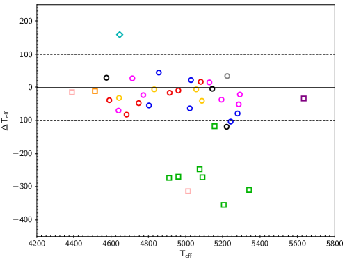
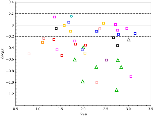
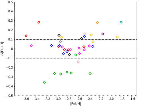
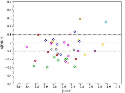
Figure 1: Comparison between this work and the literature: $\mathrm{T_{eff}}$ (upper-left panel), $\mathrm{\log g}$ (upper-right panel), Fe i (lower-left panel), and Fe ii (lower-right panel). Open circles denote $\mathrm{T_{eff}}$ and $\mathrm{\log g}$ derived from photometry, open squares denote the same derived from spectroscopy, and open triangles indicate $\mathrm{\log g}$ derived from theoretical isochrones. Data are from Barklem et al. (2005) (black), Cayrel et al. (2004) (red), Hansen et al. (2020) (cyan), Ishigaki et al. (2012) (yellow), Johnson (2002) (pink), Lai et al. (2008) (grey), Luck & Bond (1985) (orange), Mashonkina et al. (2017b) (blue), Pereira et al. (2013) (purple), Roederer et al. (2014b) (green), and Siqueira Mello et al. (2014) (magenta).

In Fig. 1 we compare our derived stellar parameters with those determined by other studies in the literature. Some stars were observed in the framework of the Large Program ‘First Stars’ (PI: R. Cayrel), and for these stars we use the results obtained in Cayrel et al. (2004) for the comparison, even if more recent values are available in literature.

In this study, we rely on Gaia EDR3 photometry and parallaxes to derive the stellar parameters (Sect. 3.2). However, in the traditional spectroscopic method, the effective temperature is obtained by requiring that there is no trend between the abundance and excitation potential of Fe i lines (i.e. excitation equilibrium). The surface gravity, instead, is obtained by requiring that Fe i and Fe ii lines provide the same abundance (i.e. ionisation equilibrium). Another way of deriving surface gravity is to use theoretical isochrones, assuming the age, metallicity, and effective temperature of the star.

As shown in Fig. 1 (upper-left panel), $\mathrm{T_{eff}}$ values in the literature appear in line with our derived temperatures, with an average $\Delta$$\mathrm{T_{eff}}$=–72 K ($\sigma$=113 K), where $\Delta$$\mathrm{T_{eff}}$=$\mathrm{T_{eff}}$(literature)-$\mathrm{T_{eff}}$(this study) is compatible with our $\pm$100 K uncertainties on $\mathrm{T_{eff}}$. One exception to this good agreement is Roederer et al. (2014b), where six out of seven stars have effective temperatures $\sim$300 K lower than our derived values. For the star CES1552+0517, Johnson (2002) also determined a $\mathrm{T_{eff}}$ $\sim$300 K lower than our derived value. As discussed in Mucciarelli & Bonifacio (2020), for metal-poor stars with [Fe/H]$\sim-2.5$, the spectroscopic $\mathrm{T_{eff}}$ and $\mathrm{\log g}$ appear to be lower than the photometric ones by $\sim$350 K and $\sim$1.0 dex, respectively. This is in agreement with the observed discrepancy.

Surface gravities in the literature appear lower than our derived values (see Fig. 1, upper-right panel), with average $\Delta$$\mathrm{\log g}$=$-0.35$ ($\sigma$=0.32). The largest discrepancy in $\mathrm{\log g}$ is found for the Roederer et al. (2014b) values, which are systematically $\sim-0.75$ dex lower than our derived $\mathrm{\log g}$. This result is not surprising, given their discrepancy with our $\mathrm{T_{eff}}$. Since Roederer et al. (2014b) determined their $\mathrm{\log g}$ using theoretical isochrones, we expect that along the red giant branch (RGB) the cooler the star, the lower is the surface gravity.

We also determined spectroscopic surface gravities for our sample stars and found that those are in agreement with literature values within 0.1 dex. The observed discrepancy between spectroscopic and photometric $\mathrm{\log g}$ seems to arise from the different iron abundance obtained from Fe i and Fe ii lines. At low metallicities, the neutral species are more affected by non-local thermodynamic equilibrium (NLTE) effects than ionised ones (e.g. Amarsi et al., 2016), which implies that the total abundance derived from each of the two species are different. Hence, when using ionisation equilibrium to derive $\mathrm{\log g}$, these over-ionisation effects can lead to an underestimation of the star’s surface gravity. A possible way to avoid this is to apply NLTE corrections before imposing ionisation equilibrium, as done in Mashonkina et al. (2017a), whose results are in good agreement with this work (blue squares in Fig. 1, upper-right panel).

In Fig. 1 (lower panels) we compare our derived chemical abundances for Fe i and Fe ii with those in literature. Our results are in general agreement with the literature abundances, with average values $\Delta$[Fe I/H]=+0.01 ($\sigma=0.15$ dex) and $\Delta$[Fe II/H]=$-0.08$ ($\sigma=0.14$ dex). We note that the [Fe/H] derived by Roederer et al. (2014b) are systematically lower than our values, which is a direct consequence of adopting lower $\mathrm{T_{eff}}$ and $\mathrm{\log g}$.

4.2 Alpha elements: Mg, Si, Ca, and Ti

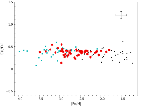
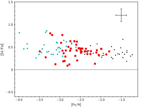
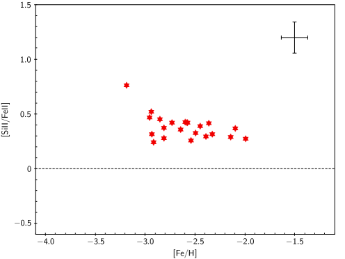
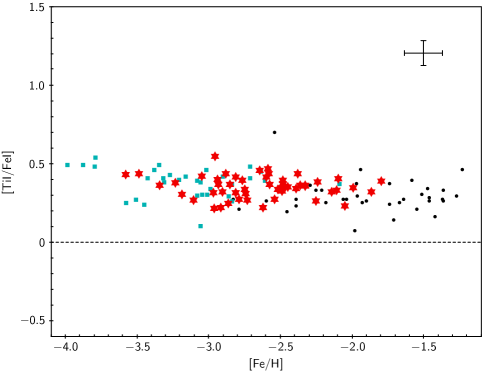
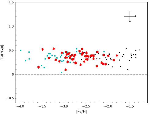
Figure 2: Elemental abundance ratios of Mg I, Si I, Si II, Ca I, Ti I, and Ti II as a function of [Fe/H] for stars in our sample (red star symbols). Cyan squares and black dots represent the same quantities for stars in Cayrel et al. (2004) and Ishigaki et al. (2012), respectively. A representative error is plotted in the upper-right corner of each panel.

Figure 2 shows the derived Mg I, Si I, Si II, Ca I, Ti I, and Ti II over Fe abundance ratios as a function of [Fe/H] for our sample of stars. Our results are compared to the values obtained by Cayrel et al. (2004) and Ishigaki et al. (2012) for giant stars in the same metallicity range. The abundance ratios of all elements are in good agreement with the results found in previous studies. All elements are enhanced respect to the Fe abundance (with sample averages and standard deviations of [Mg I/Fe I] = +0.50 $\pm$ 0.11, [Si I/Fe I] = +0.41 $\pm$ 0.16, [Si II/Fe II] = +0.38 $\pm$ 0.11, [Ca I/Fe I] = +0.37 $\pm$ 0.07, [Ti I/Fe I] = +0.35 $\pm$ 0.07, [Ti II/Fe II] = +0.35 $\pm$ 0.10), and the abundance ratios remain constant at different metallicities. The dispersion around the mean abundance ratio is equal or smaller than the mean uncertainty ($\sigma$) for Si, Ca and Ti ($\sigma_{{Si\textsc{I}}}=0.16$ dex, $\sigma_{{Si\textsc{II}}}=0.20$ dex, $\sigma_{{Ca\textsc{I}}}=0.08$ dex, $\sigma_{{Ti\textsc{I}}}=0.09$ dex, $\sigma_{{Ti\textsc{II}}}=0.11$ dex) but slightly larger for Mg ($\sigma_{{Mg\textsc{I}}}=0.07$ dex). The scatter appears to become larger at lower metallicities, as it was already observed by Cayrel et al. (2004) in their sample of stars, this is expected since at lower metallicities the lines become weaker. The error estimates are in line with what expected from the S/Ns.

We find a mean difference between [Si II/H] and [Si I/H] of $0.06\pm 0.14$ dex, and a mean difference between [Ti II/H] and [Ti I/H] of $0.13\pm 0.06$ dex. These differences are likely due to NLTE effects. Mashonkina et al. (2016a) found minimal departures from LTE for the lower levels of Si I lines typically used as abundance indicators in F-G-K stars. On the other hand, NLTE effects are particularly strong for Ti I lines (see Mashonkina et al., 2016b). According to Mashonkina et al. (2016b), for stars with stellar parameters similar to those of our targets, the NLTE corrections for Ti I are all positive, up to 0.4 dex, while the corrections for Ti II are positive and $<0.1$ dex. These values are compatible with the difference in Ti abundances observed in our stars.

4.3 Light odd-Z elements: Na and Al

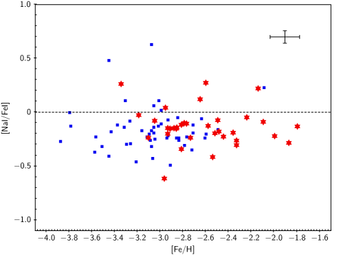
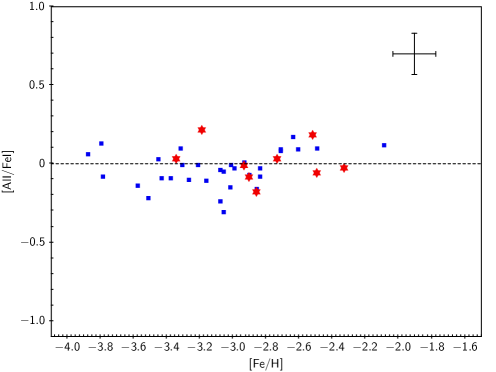
Figure 3: NLTE abundance ratios of Na and Al as a function of [Fe/H] for stars in our sample (red star symbols). Blue squares are stars from Andrievsky et al. (2007, 2008) for Na and Al, respectively. A representative error is plotted in the upper-right corner.

Sodium abundances were derived from the Na I lines at 498.3 nm, 568.2 nm, 568.8 nm, and 616.0 nm and from the Na D resonance lines at 588.9 nm (D1) and 589.5 nm (D2). As Na i lines, especially the Na i D doublet, are known for being strongly sensitive to NLTE effects (e.g. Mashonkina et al., 1993; Baumüller et al., 1998), we applied the NLTE corrections provided by Lind et al. (2011) to each line to obtain a more accurate measurement of Na abundances. The NLTE corrections for Na i lines are all negative, with an average of –0.26 dex and down to –0.57 dex for the Na i D doublet.

Aluminium abundances were derived from the Al I resonance lines at 394.4 nm and 396.1 nm. Similarly to the Na D doublet, the Al resonance doublet is sensitive to NLTE effects, and when these lines are used in LTE approximation, the derived Al abundances are severely underestimated (Baumueller & Gehren, 1997; Norris et al., 2001). To avoid this, we applied the NLTE corrections by Andrievsky et al. (2008). Nine stars in our sample have $\mathrm{T_{eff}}$ in the temperature range of the Andrievsky et al. grid, so we provide NLTE Al abundances only for these stars. The NLTE corrections are all positive, with an average of +0.63 dex.

The derived abundance ratios of Na and Al over Fe as a function of [Fe/H] are shown in Fig. 3. These are compared to the NLTE values obtained for the First Stars Large Program stars in Andrievsky et al. (2007) and Andrievsky et al. (2008), respectively. Again, our results appear in line with previous studies. The abundance ratios show a large scatter (0.17 dex for Na I, and 0.12 dex for Al I), and no clear trend with [Fe/H].

4.4 Iron-peak elements

4.4.1 Sc and V

The derived abundance ratios of [Sc I/Fe I], [Sc II/Fe II], [V I/Fe I], and [V II/Fe II] as a function of [Fe/H] are shown in Fig. 4, and compared to literature values for giant stars of similar metallicity. The mean abundance ratios and standard deviations are $-0.09\pm 0.13$ for [Sc I/Fe I], $-0.10\pm 0.10$ for [V I/Fe I], $0.15\pm 0.10$ for [Sc II/Fe II], and $0.05\pm 0.12$ dex for [V II/Fe II]. The trend appears flat down to the lowest measured [Fe/H] for both elements. This is in agreement with the results obtained by other authors.

We find a mean difference between [Sc II/H] and [Sc I/H] of $0.37\pm 0.16$ dex, and a mean difference between [V II/H] and [V I/H] of $0.27\pm 0.11$ dex. These large discrepancies seem to suggest that NLTE effects on Sc and V are important. Zhang et al. (2008) and Zhao et al. (2016) provide NLTE corrections for Sc in cool dwarf stars, but we are not currently aware of any NLTE studies of scandium conducted on metal-poor giant stars. Similarly, we are not aware of any studies that have performed NLTE corrections for V. However, we note that Ou et al. (2020) found a difference between [V II/H] and [V I/H] of $0.25\pm 0.01$ dex, which is in excellent agreement with that found in this study. Similar results have been obtained by Roederer et al. (2014b) and Hansen et al. (2020), who found higher V II than V I. We would like to stress that hyperfine splitting for Sc and V lines is not taken into account in the adopted GES line list. Roederer et al. (2014b) pointed out that the lack of hyperfine splitting for V II might lower V II abundances by $<0.1$ dex. We expect a similar behaviour for Sc II abundances. This may partially explain why we do not find an ionisation equilibrium for scandium and vanadium.

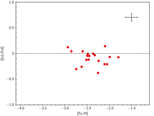
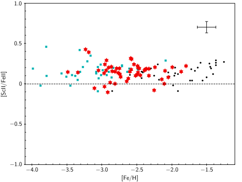
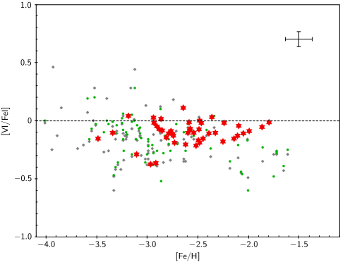
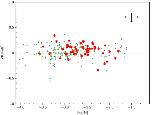
Figure 4: Elemental abundance ratios of Sc and V as a function of [Fe/H] for stars in our sample (red stars). Cyan squares and black dots represent Sc abundances for stars in the Large Program (Cayrel et al., 2004) and in Ishigaki et al. (2013), respectively. Green dots and grey diamonds represent V abundances for stars in Roederer et al. (2014b) and Ou et al. (2020), respectively. A representative error is plotted in the upper-right corner of each panel.

4.4.2 Cr and Mn

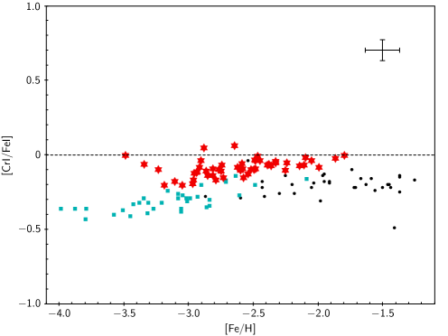
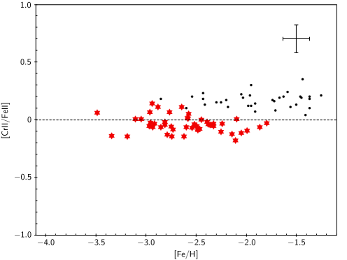
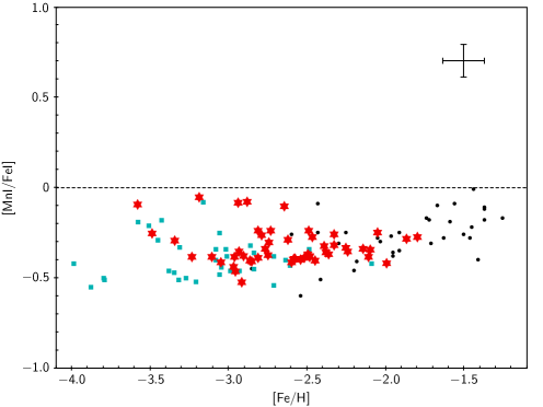
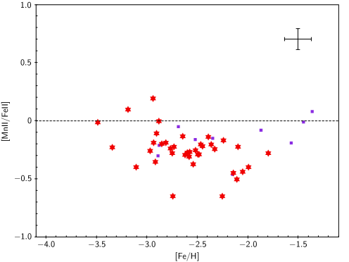
Figure 5: Elemental abundance ratios of Cr and Mn as a function of [Fe/H] for stars in our sample (red star symbols). Cyan squares and black dots are from Cayrel et al. (2004) and Ishigaki et al. (2013), respectively. Purple squares represent NLTE [Mn/Fe] abundance ratios for stars in Eitner et al. (2020). A representative error is plotted in the upper-right corner of each panel.

In Fig. 5 we compare the derived [Cr I/Fe I], [Cr II/Fe II], [Mn I/Fe I], and [Mn II/Fe II] abundance ratios to the values obtained in Cayrel et al. (2004) and in Ishigaki et al. (2013). The mean abundance ratios and standard deviations are [Cr I/Fe I]=$-0.09\pm 0.06$, [Cr II/Fe II]=$-0.04\pm 0.07$, [Mn I/Fe I]=$-0.33\pm 0.10$, and [Mn II/Fe II]=$-0.26\pm 0.17$. Contrary to Mn, for which the values found are in agreement with the literature, both [Cr I/Fe I] and [Cr II/Fe II] abundance ratios appear to differ from previous results.

For the stars that we have in common with the other studies, the derived [Cr I/Fe I] ratios are 0.17 dex and 0.12 dex higher than the values in Cayrel et al. (2004) and Ishigaki et al. (2013), respectively. On the contrary, the derived [Cr II/Fe II] ratios are 0.21 dex lower than the values in Ishigaki et al. (2013). Another difference compared to literature (see e.g. Cayrel et al., 2004; Bonifacio et al., 2009) is that the [Cr I/Fe I] ratio does not decrease with metallicity in our sample, but instead seems to increase again at the lowest observed metallicities ([Fe/H] $<-3.2$).

The difference in the [Cr I/Fe I] abundance ratios with Ishigaki et al. (2013) results seems to arise from the different Fe I abundances, as the mean [Cr I/H] is almost the same in both studies ($\Delta$[Cr I/H]$\sim 0.01$). However, we note that the mean [Cr I/H] abundance in our sample is 0.2 dex higher than in Cayrel et al. (2004). In this case, the difference in the abundance ratios is probably due to the different line selections. Cayrel et al. (2004) relied mainly on Cr I resonance lines to derive Cr abundance. In Ishigaki et al. (2013) and in this study these lines were excluded from the line list, and the same set of Cr I lines were used. To test this hypothesis, we derived the Cr I abundance for the star CES1942-6103 (CS22891-209) employing the same lines used in Cayrel et al. (2004). We obtained A(Cr I) $=2.02\pm 0.14$ dex, which is in excellent agreement with the value found by Cayrel et al. (2004) (A(Cr I) $=2.01\pm 0.16$ dex). This confirms that the Cr I abundance depends on the lines chosen for the analysis and that the observed trend with metallicity is probably due to NLTE effects, which affect each line differently. We underline that for Cr I we used $gf$ values taken from Sobeck et al. (2007), which are more recent than those used in Cayrel et al. (2004).

Similarly to the Cr I, we observe a discrepancy of –0.18 dex between our mean [Cr II/H] abundance and that of Ishigaki et al. (2013), as they adopted a different set of Cr II lines. For Cr ii we used the $gf$ values of Nilsson et al. (2006). The accuracy of the lifetimes used by these authors to derive the oscillator strengths has been questioned by Scott et al. (2015) in their solar abundance analysis. However, Sneden et al. (2016), in their analysis of the metal-poor dwarf HD 84937, showed that the use of the Nilsson et al. (2006) values considerably reduces the line-to-line scatter with respect to what was obtained using earlier $gf$ values. For this reason, we decided to keep the $gf$ values of Nilsson et al. (2006).

We find a mean difference between [Cr II/H] and [Cr I/H] of $0.18\pm 0.09$ dex, and a mean difference between [Mn II/H] and [Mn I/H] of $0.20\pm 0.10$ dex. According to Bergemann & Cescutti (2010) and Bergemann & Gehren (2008), these discrepancies are due to NLTE effects on neutral Cr and Mn. The NLTE corrections provided by Bergemann & Cescutti (2010) and Bergemann & Gehren (2008) for stars with similar parameters to those of our targets are between +0.20 and +0.60 dex for Cr I, and between +0.40 and +0.60 for Mn I. No corrections are available for the Cr II and Mn II lines we used, but we expect them to be positive and $<0.1$ dex, similar to the corrections calculated for metal-poor dwarf stars (Bergemann & Gehren, 2008; Bergemann & Cescutti, 2010; Bergemann et al., 2019). If we assume that the ionised species, which are the majority species in these stars, are formed close to LTE, the result of applying the above NLTE corrections to our Cr I and Mn I abundances would be to worsen the ionisation balance for both elements. A possible explanation is that hydrodynamical effects have not been taken into account.

For many lines of several elements the 1D NLTE corrections are positive while the 3D NLTE corrections are negative, and the full 3D NLTE correction is lower than the 1D NLTE. Bergemann et al. (2019) have computed 3D NLTE corrections for several Mn I lines and for one Mn II line. The 3D NLTE corrections for Mn I lines are positive and, surprisingly, larger than the 1D NLTE (see Fig. 17 of Bergemann et al., 2019), while the Mn II 348.8 nm line has the expected behaviour, with the 3D NLTE correction being smaller than the 1D NLTE correction. It thus seems that if the 3D NLTE corrections were applied, the ionisation balance for Mn would be worse than in LTE.

In the lower-right panel of Fig. 5, we compare our LTE Mn ii abundances with the NLTE abundances of Eitner et al. (2020). In their study, they found a difference between Mn II and Mn I between 0.1 and 0.45 dex in the LTE approximation, which is in agreement with our results. In the NLTE approximation, this discrepancy becomes lower than 0.1 dex. This is further evidence that the difference between the ionised and neutral species is due to NLTE effects that affect the Mn I lines.

4.4.3 Co, Ni, Cu, and Zn

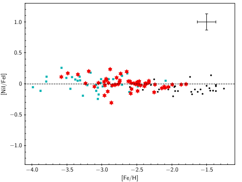
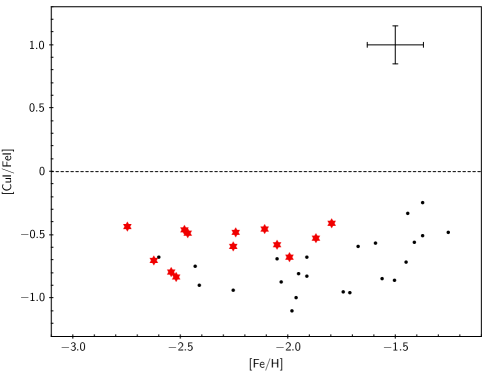
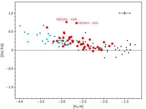
Figure 6: Elemental abundance ratios of Co, Ni, Cu, and Zn as a function of [Fe/H] for stars in our sample (red star symbols). Cyan squares and black dots represent the same quantities for stars in the Large Program (Cayrel et al., 2004) and in Ishigaki et al. (2013), respectively. A representative error is plotted in the upper-right corner of each panel.

Figure 6 shows the comparison between [Co I/Fe I], [Ni I/Fe I], [Cu I/Fe I], and [Zn I/Fe I] abundance ratios as a function of [Fe/H] for our stars and the same quantities in literature. We observe a decreasing trend with metallicity for Co and Zn, and a flat trend with a mean value around zero for Ni. Our results appear in agreement with previous studies and confirm the trend with metallicity found by other authors (Cayrel et al., 2004; Takeda et al., 2005; Lai et al., 2008; Ishigaki et al., 2013, and references therein).

Previous studies have found that the [Cu/Fe] abundance ratio decreases with decreasing metallicity in LTE (see e.g. Andrievsky et al., 2018; Roederer & Barklem, 2018; Shi et al., 2018). However, the NLTE analysis of Andrievsky et al. (2018) found that the decrease is much smaller, with [Cu/Fe]$\ga-0.3$, and for the extremely metal-poor giant CD –38 245 ([Fe/H]=–4.19) they found [Cu/Fe]=-0.07. Both our results and those of Ishigaki et al. (2013) are based on LTE and they seem to suggest that the trend with metallicity flattens out at [Fe/H]$<-1.8$ for giant stars. We note that our derived [Cu I/Fe I] ratios are $\sim 0.25$ dex higher than the values found by Ishigaki et al. (2013) for stars in the same range of metallicity. The origin of this discrepancy is not clear, since we do not have any Cu measurement in common with Ishigaki et al. (2013).

4.4.4 Zn-rich stars: CES1543+0201 and CES2254-4209

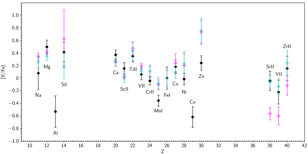
Figure 7: Elemental abundance ratios versus atomic number, Z, for stars in the sample with –3.1 $<$ [Fe/H] $<$ –2.4. Coloured symbols indicate abundance patterns for stars CES1543+0201 (magenta) and CES2254-4209 (cyan) with errors. Black symbols indicate the average abundance ratios of Zn-normal stars. Black error bars represent the standard deviation around the mean abundance. Abundance ratios of neutral and ionised species are scaled to their Fe counterpart.

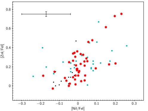
Figure 8: [Zn/Fe] versus [Ni/Fe] abundance ratios for stars in our sample (red star symbols). Cyan squares and black dots represent the same quantities for stars of similar metallicity in the Large Program (Cayrel et al., 2004) and in Ishigaki et al. (2013), respectively. A representative error is plotted in the upper-left corner.

In Fig. 6, in the panel showing [Zn/Fe], two stars stand out from the trend defined by the others and by the measurements in the literature, showing [Zn/Fe] $\sim+0.7$. CES2254–4209 (also known as HE2252–4225) was discovered in the context of the HERES survey by Mashonkina et al. (2014) as an $r-$enhanced star ([$r$/Fe]=+0.80). Mashonkina et al. (2014) found a lower enhancement for CES2254-4209 ([Zn/Fe]=+0.43), mostly due to the fact that both Fe and Zn abundances have been derived by applying NLTE corrections. The measured abundance of Th and the anomalously high Th/Eu ratio, corresponding to a radioactive age of $1.5\pm 1.5$ Gyr, classify it as an actinide boost star, a class that still only contains a handful of stars and whose prototype is CS 31082–001 (Cayrel et al., 2001; Hill et al., 2002). Such an occurrence may suggest that the overabundance of Zn is in fact due to its production through the $r$ process. However, the other Zn-rich star, CES1543+0201 (also known as CS 30312-100), initially discovered by Aoki et al. (2002), has been classified as a CEMP star ([C/Fe]=+0.98) with no enhancement of n-capture elements (CEMP-no) by Aoki et al. (2007). This star has been analysed in detail in Roederer et al. (2014b), who found a similar enhancement as in our study ([Zn/Fe]=+0.71).

In Fig. 7 we show abundance patterns for stars CES1543+0201 (magenta) and CES2254–4209 (cyan). We tried to fit these patterns with different SN yields using STARFIT (Heger & Woosley, 2010). For the lighter elements, the low mass SNe ($\sim$12 $\rm M_{\odot}$) derived by STARFIT provide reasonable fits to the observations, as quantified by $\chi^{2}$ statistics, while they fail to reproduce the observed Zn abundance, and some models also fail at explaining the Sc abundances. This is expected since such models cannot account for the neutrino-driven ejecta, where the weak $r$ process and/or the $\nu$p process may contribute to these and heavier elements.

From the abundance patterns in Fig. 7, we notice that the two Zn-rich stars also show a slight enhancement in Ni compared to the mean value observed for the sample stars of similar metallicity. In their study of Zn abundances in RGB stars of the Sculptor dwarf galaxy, Skúladóttir et al. (2017) found a correlation between Zn and Ni abundances. We checked whether this correlation was also present in our sample by performing a non-parametric Kendall’s $\tau$ test, and we found a correlation probability of 99.9%. Looking at Fig. 8, we note that the stars seem to follow two different branches in the plane for [Ni/Fe]$>$0.05. For some stars [Zn/Fe] increases with [Ni/Fe], while for the others [Zn/Fe] remains approximately constant as [Ni/Fe] increases. In our opinion, this pattern could be due to a different explosion energy of the SN for a given mass of the progenitor star (see e.g. Nomoto et al., 2013, and references therein). Hypernovae (HNe), a type of core collapse SNe with extremely large explosion energies ($\gtrsim 10^{52}$ erg), are able to produce a much larger amount of iron-peak elements, especially Zn, than classical SNe via $\alpha-$rich freeze-out (e.g. Galama et al., 1998; Iwamoto et al., 1998; Nomoto et al., 2001; Umeda & Nomoto, 2002). It is therefore possible that the Zn-rich stars in our sample formed in a gas cloud pre-enriched by HNe, while stars with approximately constant [Zn/Fe] formed from gas enriched by SNe with lower explosion energies.

4.5 Light n-capture elements: Sr, Y, and Zr

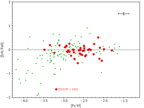
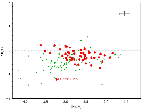
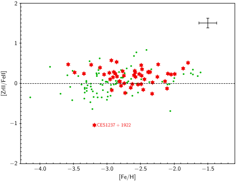
Figure 9: Elemental abundance ratios of Sr, Y, and Zr as a function of [Fe/H] for stars in our sample (red star symbols). Green dots represent Sr, Y, and Zr abundances derived in Roederer et al. (2014b). A representative error is plotted in the upper-right corner of each panel.

The derived [Sr II/Fe II], [Y II/Fe II], and [Zr II/Fe II] abundance ratios as a function of [Fe/H] are shown in Fig. 9, and compared to literature values for giant stars of similar metallicity. Our results appear in general agreement with previous studies. For stars in Roederer et al. (2014b), we note that for [Fe/H]¡$-3.0$ the dispersions around the mean value become larger and the abundance ratios of Sr and Y seem to decrease with metallicity. These trends have also been observed in other studies (see e.g. François et al., 2007). This is not the case for our targets, for which the trend remains approximately flat at these metallicities, with sample averages and standard deviations of [Sr II/Fe II]=$-0.08\pm 0.32$, [Y II/Fe II]=$-0.24\pm 0.25$, and [Zr II/Fe II]=$+0.16\pm 0.26$. We stress the fact that, at metallicities below –3, we only have measurements for about five stars in our sample, so it is possible that this difference in trend with the literature could be due to poor statistics.

For the seven stars for which we were able to measure Zr I, we find a mean difference between [Zr II/H] and [Zr I/H] of $0.57\pm 0.09$ dex. We suspect that this difference is due to strong NLTE effects. According to Velichko et al. (2010), NLTE corrections for Zr II are $\sim$ +0.2 dex for giant stars with [Fe/H] $\sim$ –3. At solar metallicity, the NLTE corrections for Zr I are about +0.3 dex, while no correction is available for metal-poor stars.

5 Discussion

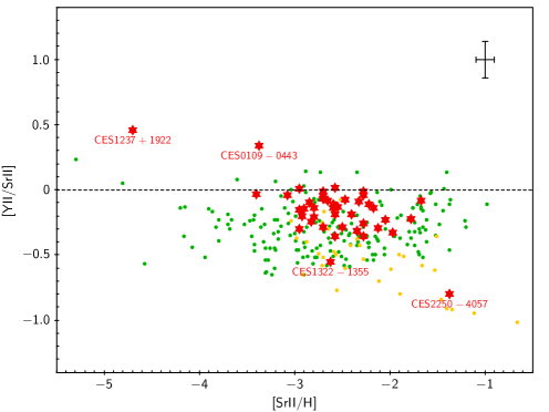
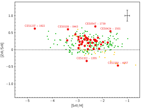
Figure 10: [Y II/Sr II] and [Zr II/Sr II] as a function of [Sr II/H] for stars in our sample (red star symbols). Green dots represent the same quantities derived for main sequence, RGB, and sub-giant stars in the Roederer et al. (2014b) sample. Yellow dots are the same quantities derived for horizontal branch stars in the Roederer et al. (2014b) sample. A representative error is plotted in the upper-right corner of each panel.

Figure 11: Normalised spectra of stars CES1237+1922 (red) and CES1322–1355 (black) around the Sr II line at 421.5 nm (left panel), the Y II line at 378.8 nm (central panel), and the Zr II line at 383.6 nm (right panel). The stars have similar stellar parameters ($\mathrm{T_{eff}}$=4960, $\mathrm{\log g}$=1.8, $\mathrm{v_{turb}}$=1.9, [Fe/H]=–3).

The abundances of Sr, Y, and Zr are critical to constrain the astrophysical conditions of their production site once nuclear physics uncertainties are reduced (Psaltis et al., 2022). The variations in the observationally derived abundances could be due to differences in the analysis as described above; therefore, it is important to have homogeneously derived abundances for a large number of stars, as we presented here. In homogeneous analyses, the variations found in the observations can be linked to different astrophysical conditions and thus be used to constrain the site. A potential contribution to Sr, Y, and Zr are neutrino-driven ejecta in core-collapse SNe, where changes in the conditions (entropy, neutron richness, and expansion timescale) result in different patterns (see e.g. Hansen et al., 2014b). Since Sr, Y, and Zr are produced in SNe by a process that runs close to stability, the nuclear physics uncertainties are small or can be constrained by experiments in the near future. Therefore, homogeneous abundances of the lighter heavy elements are a strong diagnostic for the conditions in SN explosions.

In Fig. 10 we note that there are stars that show a [Y II/Sr II] and [Zr II/Sr II] ratio that is different, higher or lower, from the average of the other stars in the sample. In the following subsections we present these peculiar stars, and defer a deeper discussion on their abundance pattern in future articles, when a more complete inventory of the n-capture element abundances will be available.

5.1 CES1237+1922

The star CES1237+1922 (also known as BS 16085-0050) is deficient in Sr, Y and Zr compared to stars of similar metallicity (see Fig. 9 and 11), with A(Sr II)=$-1.78\pm 0.04$ ([Sr II/Fe II]=$-1.66$), A(Y II)=$-2.03\pm 0.05$ ([Y II/Fe II]=$-1.21$), and A(Zr II)=$-1.46\pm 0.12$ ([Zr II/Fe II]=$-1.04$). The chemical composition of this star was first studied by Giridhar et al. (2001), who noted it for being rich in $\alpha$-elements. This finding is confirmed by our analysis, as for this star we derived A(Mg I)=$+5.12\pm 0.04$ ([Mg I/Fe I]=$+0.77$) and A(Ca I)=$+3.68\pm 0.10$ ([Ca I/Fe I]=$+0.54$). Sr abundance derived by Giridhar et al. (2001) was low, and so was that in Honda et al. (2004). This is essentially in line with our analysis, once the lower gravity adopted by Giridhar et al. (2001) is accounted for, with respect to ours and that of Honda et al. (2004). There are very few stars that have such low abundances of all three elements that populate the first peak of n-capture elements. We looked for stars with similar light n-capture elements abundances as CES1237+1922 in the SAGA database (Suda et al., 2008). We found that there are only seven stars with similar Sr and Y abundances, and only two of these have a measurement of Zr.

Figure 10 shows how CES1237+1922 stands out with respect to the rest of our sample (see also Figs. 1 and 3 of François et al., 2007). Qian & Wasserburg (2008) noted the difficulty in explaining the stars with low abundances of first peak elements. In a scenario in which all n-capture elements are formed via the $r$ process, they invoked three distinct $r-$process sites to explain the observations. Faint SNe, with mixing and fall-back (Iwamoto et al., 2005), are appealing sites since they show an excess of hydrostatic burning products with respect to the explosive products, thus explaining the exceptional stars with very low [Sr,Y,Zr/Fe].

Several studies have shown that the observed abundances of the first peak elements and that of second peak elements in low metallicity stars require the existence of at least two sites for n-capture nucleosynthesis (e.g. Hansen et al., 2012, 2014a, 2014b; Spite et al., 2018). The Galactic chemical evolution models of Prantzos et al. (2018) seem incapable of producing low [Sr/Fe], [Y/Fe] and [Zr/Fe] ratios as observed in CES1237+1922, even in the unrealistic hypothesis of switching off completely the $r-$process contribution.

Another possibility would be that the $\alpha-$elements and Sr, Y, and Zr are produced in a neutrino-driven SN, while heavy n-capture elements (second peak and heavier) come from an $r-$process event where first peak elements are underproduced compared to heavier ones, like, for example, neutron star merger dynamical ejecta (Korobkin et al., 2012) and disk ejecta (Wu et al., 2016). The low abundance of Sr, Y, and Zr relative to the iron-group elements could point to proton-rich ejecta from SN explosions. Under such conditions, the $\nu$p process can also produce Sr, Y, and Zr; however, their abundances are low relative to the iron-group nuclei (Hansen et al., 2014b; Fröhlich et al., 2006; Wanajo, 2006; Pruet et al., 2006).

5.2 CES0109-0443

CES0109-0443 (also known as CS 22183-031) is underabundant in Sr with respect to Y and Zr, with [Y II/Sr II]=+0.34 and [Zr II/Sr II]=+0.59 (Fig. 10). This star was identified for the first time as an $r$-process-enhanced metal-poor star by Honda et al. (2004), with [Eu/Fe]=+1.2. It has also been analysed in detail by Roederer et al. (2014b), who confirmed the high enhancement in $r-$process material (Roederer et al., 2014b, a). For this star Roederer et al. (2014b) derived A(Sr)=$-0.84$ dex, A(Y)=$-1.61$ dex, and A(Zr)=$-0.7$ dex, which are significantly lower than those found in this study (A(Sr)=$-0.45\pm 0.07$ dex, A(Y)=$-0.82\pm 0.14$ dex, and A(Zr)=$-0.16\pm 0.06$ dex). Since the lines used in our study and in Roederer et al. (2014b) are approximately the same but the parameters are different, we derived the abundances of these elements using the parameters obtained in Roederer et al. (2014b), and we found that our results are consistent with theirs. We conclude that the origin of the discrepancy is only due to the different choice of stellar parameters.

5.3 CES2250–4057 and CES1322–1355

The star CES2250–4057 (also known as CD-41 15048 also known as HE 2247-4113) is overabundant in Sr with respect to Y and Zr, with [Y II/Sr II]=$-0.80$ and [Zr II/Sr II]=$-0.46$ (Fig. 10). For this star we derived A(Sr II)=$+1.55\pm 0.07$ ([Sr II/Fe II]=$+0.51$), A(Y II)=$+0.04\pm 0.09$ ([Y II/Fe II]=$-0.29$), and A(Zr II)=$+0.79\pm 0.06$ ([Zr II/Fe II]=$+0.05$). This pattern is striking in our sample, and more generally in the literature, with about a dozen stars showing a similar behaviour. This star is one of the Bidelman-MacConnell ‘weak-metal’ stars (Bidelman & MacConnell, 1973; Norris et al., 1985). It is a red horizontal branch star and has been studied by Pereira et al. (2013) as a potential star that is escaping the Galaxy. They do not measure Sr, but their Y and Zr abundances are compatible with ours, within errors, especially after the 0.6 dex lower gravity is accounted for. So this overabundance of Sr has not been noted before. In Fig. 10 we highlighted with yellow dots the horizontal branch stars in Roederer et al. (2014b). The star CES2250–4057 lies in the region occupied by other red horizontal branch stars.

There is another, slightly milder, case of this behaviour in our sample (Fig. 10), CES1322–1355 (also known as HE 1320–1339), for which we derived A(Sr II)=$+0.30\pm 0.05$ ([Sr II/Fe II]=$+0.16$), A(Y II)=$-0.96\pm 0.13$ ([Y II/Fe II]=$-0.40$), and A(Zr II)=$-0.33\pm 0.07$ ([Zr II/Fe II]=$-0.17$). This star was initially studied within the HERES survey (Barklem et al., 2005), who found [Sr/Fe]$=+0.23\pm 0.16$ and [Y/Fe]$=-0.13\pm 0.15$. This star has been analysed also by Sakari et al. (2018) who provide [Sr/Fe]$=+0.50\pm 0.14$. Our results are in line with previous studies once we take the different choice of stellar parameters into account. Sakari et al. (2018) classified this star as limited-r, a classification introduced by Frebel (2018) ([Eu/Fe] $<0.3$, [Sr/Ba] $>0.5$, and [Sr/Eu] $>0.0$) with the aim of capturing the stars enriched under the condition of low neutron-to-seed ratios, a process more often referred to as ‘weak-r’ process. Yet since they do not have measurements of Y and Zr, Sakari et al. (2018) did not note the overabundance of Sr ([Y II/Sr II]=$-0.55$ and [Zr II/Sr II]=$-0.33$).

5.4 CES0547-1739 and CES0424-1501

Looking at the right panel in Fig. 10, we note that there are two stars (CES0547-1739 and CES0424-1501) with an overabundance of Zr with respect to Sr and Y, with [Zr II/Sr II]=$+0.68$ and [Zr II/Y II]=$+0.70$ for CES0547-1739, and [Zr II/Sr II]=$+0.54$ and [Zr II/Y II]=$+0.62$ for CES0424-1501. Star CES0547-1739 (also known as TYC 5922-517-1) has previously been observed by the GALAH survey, which provided stellar parameters and chemical abundances for some elements (Martell et al., 2017; Buder et al., 2018). As no Sr and Zr abundance is present in the literature for this star, we provide them in this study for the first time. Star CES0424-1501 (also known as BD-15 779) has been studied in detail by Hansen et al. (2020), who found [Zr/Sr]$=+0.38$ and [Zr/Y]$=+0.68$. These results are compatible with ours taking into account the uncertainties and the difference in stellar parameters.

6 Conclusions

In this study we present a homogeneous set of stellar parameters and a chemical abundance analysis of elements from Na to Zr for a sample of 52 Galactic halo giant stars with $-3.58\leq$ [Fe/H] $\leq-1.79$. We compared our results to the ones in the literature and find a good agreement with previous studies. For stars that have a few chemical abundances in the literature, we completed the chemical inventory of light elements.

The main conclusions of this study are the following:

• For 22 stars we were able to measure the Si II abundances thanks to the high S/N and resolution of our dataset. Similar measures are not available in the literature for these stars. Quite interestingly, Si is very close to ionisation balance, with our parallax-based gravities, which suggests that either the NLTE effects are not large or they are similar for the neutral and singly ionised lines. This is in agreement with the results obtained by Amarsi et al. (2020), who find that NLTE effects on Si are small for stars in the GALAH survey, although the metallicity of the stars in their sample is higher than ours.

• We were able to measure Sc I in 19 metal-poor giants, again a novelty with respect to previous studies. The ionisation imbalance is on average 0.37 dex. It would be interesting to study NLTE effects on Sc I to see if this is the cause of the ionisation imbalance.

• For Cr we have a very important result: for our choice of lines we find a flat trend of [Cr/Fe] $\approx 0$, both for the neutral and the singly ionised species, in our LTE treatment. This trend is theoretically expected since Cr and Fe are both formed under the same physical conditions. Previous investigations (e.g. McWilliam et al., 1995; Cayrel et al., 2004) relied heavily on Cr I resonance lines, which are strongly affected by NLTE effects. This has been observationally confirmed by Bonifacio et al. (2009), who find that, for their sample of extremely metal-poor giants, the [Cr ii/Fe] is around zero, while [Cr i/Fe] decreases with decreasing metallicity, suggesting NLTE effects on the Cr i lines. This is supported by the large scatter in Cr abundances, both from ionised and neutral species, from chemical studies of individual stars (Sneden et al., 2016).

• We were able to measure Mn II abundances for 38 stars; again, this measure is not generally available. Existing NLTE and 3D NLTE computations do not seem able to explain the ionisation imbalance and in fact seem to worsen it. Further theoretical investigation of the line formation of Mn I and Mn II stars is desirable.

• We have roughly doubled the number of measurements of Cu in the metallicity regime [Fe/H] $\leq-2.5$.

• We highlighted the existence of two Zn-rich stars in the sample. Both stars were previously known, and our measurements are consistent with the literature. The fact that one of the two stars (CES2254–4209) is rich in $r$-process elements (and is in fact an actinide boost star) while the other (CES1543+0201) is not essentially rules out the hypothesis that this enhancement is due to the production of Zn through neutron captures.

• We noted the existence of two branches in the [Zn/Fe] versus [Ni/Fe] plane and suggest that the high [Zn/Fe] branch is due to a contribution of HNe to the chemical enrichment of the gas out of which the stars were formed. These two branches are also present in the (Cayrel et al., 2004) sample, but they were not reported before. Our data help make the presence of the two branches more obvious.

• The measurement of Sr, Y, and Zr highlighted several stars with a peculiar pattern. CES1237+1922 is deficient in all three elements compared to the other stars in the sample. CES2250-4057 shows abundances of Y and Zr that are compatible with those of other stars with similar metallicity; however, [Sr/H] is about 1 dex more abundant than [Y/H] and [Zr/H], making the production site of Sr - Zr far from clear.

The high quality of our spectra, both in terms of S/N and resolving power, allowed us to measure many weak lines that are in general not measured in stars in this metallicity range. In this way, we provided a unique sample of measures of Si II, Sc I, and Mn II. These observations can provide important guidelines in the development of line formation computations, more sophisticated than those presented here, that take deviations from LTE and hydrodynamical effects into account.

The homogeneity of our analysis was crucial in highlighting any chemical peculiarities in the stars of our sample. Stellar parameters derived in this study will be used to determine the heavy n-capture element abundances in future papers of this project, and this will allow us to draw more conclusions about the chemistry of these peculiar stars.

Appendix A Observation log

Table 5: Observation log.

Name ID	CERES name	RA2000	DEC2000	UVES arm	R	$\mathrm{v_{broad}}$	Date	MJD	exp. time	S/N	slit
						$\mathrm{km\,s^{-1}}$			s	px-1	”
HD2796	CES0031-1647	00:31:16.91	-16:47:40.8	BLU390	71050	7.2	2005-11-18	53692.01	300	123	0.4
				RED580	107200	7.3	2005-11-18	53692.01	300	259	0.3
HD4306	CES0045-0932	00:45:27.16	-09:32:39.8	BLU346	40970	7.7	2001-10-09	52191.14	697	131	1.0
							2001-10-09	52191.12	660	126	1.0
							2001-10-09	52191.12	660	134	1.0
							2001-10-09	52191.13	697	129	1.0
							2001-10-09	52191.11	660	129	1.0
				RED580	56990	6.9	2001-10-09	52191.11	305	241	0.7
							2001-10-09	52191.12	305	233	0.7
							2001-10-09	52191.13	305	261	0.7
							2001-10-09	52191.11	305	244	0.7
							2001-10-09	52191.12	305	240	0.7
							2001-10-09	52191.12	305	239	0.7
BD-11_145	CES0048-1041	00:48:24.31	-10:41:30.9	BLU390	40970	8.8	2019-11-19	58806.05	2200	128	1.0
				RED564	42310	8.0	2019-11-19	58806.05	2200	0	1.0
HD5426	CES0055-3345	00:55:41.05	-33:45:11.5	BLU390	40970	7.0	2019-11-20	58807.05	900	160	1.0
				RED564	42310	6.4	2019-11-20	58807.05	900	360	1.0
HE0057-4541	CES0059-4524	00:59:59.28	-45:24:53.4	BLU390	40970	6.7	2007-11-07	54411.04	3600	24	1.0
							2007-11-07	54411.14	3600	24	1.0
							2007-11-07	54411.10	3600	26	1.0
							2007-11-07	54411.18	3600	23	1.0
							2007-11-08	54412.23	3600	21	1.0
							2007-11-08	54412.18	3600	26	1.0
BPSCS22953-003	CES0102-6143	01:02:15.87	-61:43:45.8	BLU390	49620	8.2	2002-08-03	52489.18	1800	18	0.8
							2002-08-03	52489.20	1800	20	0.8
				RED564	87410	6.8	2002-08-03	52489.18	1800	19	0.4
							2002-08-03	52489.20	1800	21	0.4
HE0105-6141	CES0107-6125	01:07:37.85	-61:25:17.7	BLU390	40970	6.6	2007-11-09	54413.22	4500	30	1.0
BPSCS22183-031	CES0109-0443	01:09:05.09	-04:43:21.3	BLU390	40970	7.1	2017-09-26	58022.22	3005	62	1.0
HD13979	CES0215-2554	02:15:20.85	-25:54:54.9	BLU390	40970	8.4	2019-11-19	58806.18	600	147	1.0
				RED564	42310	8.6	2019-11-19	58806.18	600	330	1.0
BD-22_395	CES0221-2130	02:21:57.94	-21:30:43.0	BLU390	40970	8.7	2019-11-20	58807.07	2200	141	1.0
				RED564	42310	8.8	2019-11-20	58807.07	2200	357	1.0
HE0240-0807	CES0242-0754	02:42:57.73	-07:54:35.4	BLU390	40970	8.0	2007-11-07	54411.23	3600	19	1.0
							2007-11-08	54412.27	4500	16	1.0
							2007-11-10	54414.07	3600	17	1.0
							2007-11-10	54414.03	3600	12	1.0
							2007-11-10	54414.11	3600	18	1.0
							2007-11-10	54414.21	3600	19	1.0
							2007-11-10	54414.17	3600	19	1.0
							2007-11-10	54414.25	3600	15	1.0
BPSCS31078-018	CES0301+0616	03:01:00.69	+06:16:31.8	BLU390	40970	6.7	2019-11-19	58806.08	4200	57	1.0
							2019-11-19	58806.13	4200	59	1.0
				BLU390	40970	6.7	2017-10-01	58027.19	3005	65	1.0
				RED564	42310	6.2	2019-11-19	58806.08	4200	141	1.0
							2019-11-19	58806.13	4200	142	1.0
HE0336-2412	CES0338-2402	03:38:41.49	-24:02:50.3	BLU346	40970	6.7	2001-12-13	52256.14	1175	122	1.0
							2001-12-13	52256.15	1175	122	1.0
							2001-12-13	52256.05	1475	121	1.0
							2001-12-13	52256.18	1175	111	1.0
							2001-12-13	52256.17	1175	119	1.0
							2001-12-13	52256.03	1475	124	1.0
				RED580	56990	6.3	2001-12-13	52256.15	560	180	0.7
							2001-12-13	52256.16	560	165	0.7
							2001-12-13	52256.14	560	165	0.7
							2001-12-13	52256.15	560	180	0.7
							2001-12-13	52256.19	560	163	0.7
							2001-12-13	52256.17	560	166	0.7
							2001-12-13	52256.17	560	175	0.7
							2001-12-13	52256.18	560	159	0.7
BD+06_648	CES0413+0636	04:13:13.11	+06:36:01.8	BLU390	40970	9.7	2019-11-20	58807.21	600	70	1.0
				RED564	42310	8.4	2019-11-20	58807.21	600	322	1.0
BPSCS22186-023	CES0419-3651	04:19:45.53	-36:51:36.0	BLU390	40970	7.5	2006-10-18	54026.30	2400	60	1.0
							2019-11-19	58806.21	3600	64	1.0
							2019-11-19	58806.25	3600	52	1.0
				RED564	42310	7.6	2019-11-19	58806.21	3600	144	1.0
							2019-11-19	58806.25	3600	122	1.0
							2006-10-18	54026.30	2400	137	1.0
HD27928	CES0422-3715	04:22:55.14	-37:15:49.2	BLU390	40970	7.2	2019-11-19	58806.20	900	148	1.0
				RED564	42310	7.3	2019-11-19	58806.20	900	333	1.0
BD-15_779	CES0424-1501	04:24:45.64	-15:01:50.7	BLU390	40970	8.0	2020-03-02	58910.99	2700	157	1.0
				RED564	42310	7.6	2020-03-02	58910.99	2700	506	1.0
HE0428-1340	CES0430-1334	04:30:51.42	-13:34:08.1	BLU390	40970	7.2	2019-11-20	58807.13	1800	159	1.0
				RED564	42310	7.7	2019-11-20	58807.13	1800	344	1.0
HE0442-1234	CES0444-1228	04:44:51.71	-12:28:45.5	BLU390	58640	7.4	2003-02-05	52675.11	3600	37	0.6
							2003-02-05	52675.15	3197	28	0.6
							2003-02-05	52675.06	3600	35	0.6
							2003-02-06	52676.06	3600	44	0.6
							2003-02-06	52676.11	3600	39	0.6
							2003-02-08	52678.12	3600	31	0.6
				RED580	66320	7.3	2003-02-05	52675.06	3600	129	0.6
							2003-02-05	52675.15	3205	114	0.6
							2003-02-05	52675.11	3600	136	0.6
							2003-02-06	52676.06	3600	149	0.6
							2003-02-06	52676.11	3600	139	0.6
							2003-02-08	52678.12	3600	124	0.6
HE0516-3820	CES0518-3817	05:18:12.92	-38:17:32.7	BLU390	40970	6.7	2007-11-09	54413.33	3600	29	1.0
HE0524-2055	CES0527-2052	05:27:04.44	-20:52:42.1	BLU390	40970	8.3	2007-11-07	54411.32	3600	38	1.0
							2007-11-07	54411.28	3600	39	1.0
							2007-11-08	54412.33	3300	25	1.0
							2007-11-10	54414.30	3600	30	1.0
TYC5922-517-1	CES0547-1739	05:47:20.81	-17:39:41.0	BLU390	40970	10.0	2019-11-20	58807.23	4080	49	1.0
							2019-11-20	58807.27	4080	43	1.0
				RED564	42310	8.4	2019-11-20	58807.23	4080	224	1.0
							2019-11-20	58807.27	4080	204	1.0
TYC4840-159-1	CES0747-0405	07:47:15.82	-04:05:46.1	BLU390	40970	11.2	2020-03-03	58911.03	2500	38	1.0
							2020-03-03	58911.06	2500	36	1.0
							2020-03-04	58912.02	1800	28	1.0
							2020-03-04	58912.04	1800	31	1.0
				RED564	42310	10.0	2020-03-03	58911.03	2500	267	1.0
							2020-03-03	58911.05	2500	259	1.0
							2020-03-04	58912.02	1800	215	1.0
							2020-03-04	58912.04	1800	229	1.0
TYC8931-1111-1	CES0900-6222	09:00:52.59	-62:22:52.8	BLU390	40970	8.9	2019-11-19	58806.30	4200	53	1.0
							2019-11-20	58807.33	2200	25	1.0
				RED564	42310	8.2	2019-11-19	58806.30	4200	278	1.0
							2019-11-20	58807.33	2200	161	1.0
TYC8939-2532-1	CES0908-6607	09:08:07.51	-66:07:33.9	BLU390	40970	8.8	2020-03-04	58912.19	3600	60	1.0
				RED564	42310	9.1	2020-03-04	58912.19	3600	250	1.0
TYC9200-2292-1	CES0919-6958	09:19:16.29	-69:58:39.9	BLU390	40970	8.9	2020-03-04	58912.15	3600	50	1.0
				RED564	42310	7.6	2020-03-04	58912.15	3600	242	1.0
UCAC2_1106907	CES1116-7250	11:16:54.01	-72:50:16.1	BLU390	40970	10.3	2020-03-04	58912.23	3600	24	1.0
				RED564	42310	9.4	2020-03-04	58912.23	3600	213	1.0
HE1219-0312	CES1221-0328	12:21:34.14	-03:28:39.6	BLU346	58640	5.6	2004-02-20	53055.33	3600	6	0.6
							2004-02-20	53055.37	3600	5	0.6
							2004-02-20	53055.28	3600	6	0.6
							2004-04-16	53111.07	1198	1	0.6
							2004-05-11	53136.02	3600	6	0.6
							2004-05-11	53136.06	3600	6	0.6
							2004-05-24	53149.09	3600	4	0.6
							2004-05-23	53149.00	3600	4	0.6
							2004-05-24	53149.04	3600	4	0.6
							2005-01-19	53389.32	3600	6	0.6
							2005-04-08	53468.12	3600	6	0.6
							2005-04-08	53468.16	3600	6	0.6
							2005-04-08	53468.21	3600	6	0.6
							2005-04-10	53470.18	3600	7	0.6
							2005-04-10	53470.13	3600	6	0.6
							2005-04-10	53470.09	3600	6	0.6
							2005-04-11	53471.10	3600	6	0.6
							2005-04-11	53471.15	3600	5	0.6
				RED580	66320	6.4	2004-02-20	53055.28	3600	36	0.6
							2004-02-20	53055.33	3600	34	0.6
							2004-02-20	53055.37	3600	33	0.6
							2004-04-16	53111.07	1201	15	0.6
							2004-05-11	53136.02	3600	34	0.6
							2004-05-11	53136.06	3600	35	0.6
							2004-05-24	53149.09	3600	29	0.6
							2004-05-23	53149.00	3600	29	0.6
							2004-05-24	53149.04	3600	29	0.6
							2005-01-19	53389.32	3600	35	0.6
							2005-04-08	53468.16	3600	35	0.6
							2005-04-08	53468.12	3600	35	0.6
							2005-04-08	53468.21	3600	34	0.6
							2005-04-10	53470.13	3600	36	0.6
							2005-04-10	53470.09	3600	33	0.6
							2005-04-10	53470.18	3600	37	0.6
							2005-04-11	53471.10	3600	34	0.6
							2005-04-11	53471.15	3600	33	0.6
HD107752	CES1222+1136	12:22:52.72	+11:36:25.5	BLU390	40970	8.0	2020-03-03	58911.22	2400	163	1.0
							2020-03-03	58911.25	2400	163	1.0
				RED564	42310	8.1	2020-03-03	58911.22	2400	426	1.0
							2020-03-03	58911.25	2400	424	1.0
HD108317	CES1226+0518	12:26:36.83	+05:18:09.0	BLU346	40970	7.7	2002-02-04	52309.29	260	154	1.0
							2002-02-04	52309.29	260	127	1.0
							2002-02-04	52309.30	260	160	1.0
							2002-02-04	52309.31	260	155	1.0
							2002-02-04	52309.29	250	158	1.0
							2002-02-04	52309.30	260	132	1.0
							2002-02-04	52309.28	250	161	1.0
				RED580	56990	6.3	2002-02-04	52309.30	107	232	0.7
							2002-02-04	52309.30	107	170	0.7
							2002-02-04	52309.29	107	200	0.7
							2002-02-04	52309.30	107	182	0.7
							2002-02-04	52309.29	107	186	0.7
							2002-02-04	52309.30	107	202	0.7
							2002-02-04	52309.31	107	218	0.7
							2002-02-04	52309.30	107	168	0.7
							2002-02-04	52309.29	107	222	0.7
							2002-02-04	52309.31	107	205	0.7
HD108577	CES1228+1220	12:28:16.86	+12:20:41.1	BLU390	40970	8.8	2020-03-03	58911.20	1100	147	1.0
				RED564	42310	8.9	2020-03-03	58911.20	1100	359	1.0
BPSBS16085-0050	CES1237+1922	12:37:46.68	+19:22:49.6	BLU390	40970	7.9	2020-03-04	58912.28	3000	76	1.0
							2020-03-04	58912.32	3000	76	1.0
				RED564	42310	8.0	2020-03-04	58912.28	3000	182	1.0
							2020-03-04	58912.32	3000	189	1.0
HE1243-2408	CES1245-2425	12:45:53.85	-24:25:02.4	BLU390	40970	7.5	2020-03-03	58911.12	3250	133	1.0
							2020-03-03	58911.16	3250	138	1.0
				RED564	42310	7.6	2020-03-03	58911.12	3250	342	1.0
							2020-03-03	58911.16	3250	346	1.0
HE1320-1339	CES1322-1355	13:22:44.11	-13:55:31.4	BLU390	40970	8.3	2020-03-03	58911.28	2600	141	1.0
							2020-03-03	58911.31	2600	149	1.0
				RED564	42310	8.3	2020-03-03	58911.28	2600	340	1.0
							2020-03-03	58911.31	2600	358	1.0
HD122563	CES1402+0941	14:02:31.85	+09:41:09.9	BLU346	65030	7.0	2002-02-19	52324.39	86	84	0.5
							2002-02-19	52324.39	86	96	0.5
				RED564	51690	8.0	2000-04-12	51646.27	60	431	0.8
							2000-04-12	51646.27	60	413	0.8
							2000-04-12	51646.27	60	407	0.8
HD122956	CES1405-1451	14:05:13.02	-14:51:25.5	BLU346	40970	8.6	2003-06-07	52797.97	250	109	1.0
				RED564	42310	8.3	2000-04-12	51646.33	120	362	1.0
							2000-04-12	51646.34	120	376	1.0
TYC9427-1414-1	CES1413-7609	14:13:11.18	-76:09:50.4	BLU390	40970	8.1	2020-03-04	58912.36	2800	111	1.0
				RED564	42310	7.7	2020-03-04	58912.36	2800	341	1.0
HD126587	CES1427-2214	14:27:00.36	-22:14:39.0	BLU346	40970	7.6	2002-03-22	52355.33	836	178	1.0
							2002-03-22	52355.32	836	170	1.0
							2002-03-22	52355.34	836	170	1.0
							2002-03-22	52355.31	836	172	1.0
							2002-03-23	52356.32	827	161	1.0
							2002-03-23	52356.31	827	164	1.0
				RED580	56990	7.0	2002-03-22	52355.32	390	293	0.7
							2002-03-22	52355.31	390	303	0.7
							2002-03-22	52355.33	390	306	0.7
							2002-03-22	52355.34	390	301	0.7
							2002-03-22	52355.32	390	290	0.7
							2002-03-22	52355.34	390	288	0.7
							2002-03-22	52355.31	390	288	0.7
							2002-03-22	52355.33	390	307	0.7
HD128279	CES1436-2906	14:36:48.51	-29:06:46.6	BLU346	40970	5.9	2003-08-07	52858.99	800	252	1.0
				BLU346	40970	5.9	2002-02-04	52309.36	250	190	1.0
							2002-02-04	52309.36	250	184	1.0
							2002-02-04	52309.36	250	191	1.0
				RED564	42310	6.8	2000-04-12	51646.32	600	551	1.0
BPSCS30312-100	CES1543+0201	15:43:31.66	+02:01:17.3	BLU390	40970	6.9	2006-03-20	53814.39	900	27	1.0
							2006-03-20	53814.38	900	29	1.0
							2006-03-20	53814.40	900	28	1.0
				RED580	42310	6.5	2006-03-20	53814.4	900	76	1.0
							2006-03-20	53814.38	900	77	1.0
							2006-03-20	53814.39	900	74	1.0
BD+05_3098	CES1552+0517	15:52:17.26	+05:17:44.3	BLU390	40970	6.9	2020-03-03	58911.34	2200	148	1.0
				RED564	42310	7.1	2020-03-03	58911.34	2200	359	1.0
BD+23_3130	CES1732+2344	17:32:41.62	+23:44:11.6	BLU390	49620	6.3	2000-04-16	51650.35	600	151	0.8
							2000-04-16	51650.34	600	151	0.8
							2000-04-16	51650.33	600	155	0.8
HD165195	CES1804+0346	18:04:40.07	+03:46:44.7	BLU346	40970	9.3	2003-09-07	52889.02	625	108	1.0
				RED564	42310	8.5	2000-04-12	51646.36	120	352	1.0
							2000-04-12	51646.36	120	370	1.0
BPSCS22891-209	CES1942-6103	19:42:02.18	-61:03:44.5	BLU390	40970	7.7	2006-10-15	54023.97	1200	44	1.0
				RED580	42310	8.6	2006-10-15	54023.97	1200	133	1.0
BPSCS22873-166	CES2019-6130	20:19:22.04	-61:30:15.1	BLU390	40970	8.6	2006-10-17	54025.98	600	25	1.0
				RED580	42310	8.9	2006-10-17	54025.98	600	95	1.0
BPSCS22897-008	CES2103-6505	21:03:11.86	-65:05:08.9	BLU346	53750	7.3	2008-04-22	54578.36	5200	30	0.7
							2008-05-12	54598.36	5200	30	0.7
							2008-05-22	54608.26	5200	28	0.7
							2008-06-24	54641.36	5200	18	0.7
							2008-06-24	54641.30	5200	19	0.7
							2008-06-27	54644.17	5200	19	0.7
BPSCS29491-069	CES2231-3238	22:31:02.19	-32:38:36.5	BLU390	71050	4.5	2005-11-20	53694.08	3600	40	0.4
							2005-11-20	53694.12	3600	39	0.4
				RED580	51690	6.9	2004-10-03	53281.00	3600	119	0.8
HE2229-4153	CES2232-4138	22:32:49.05	-41:38:25.2	BLU390	40970	7.1	2007-11-08	54412.05	2700	52	1.0
							2007-11-09	54413.01	2700	27	1.0
							2007-11-09	54413.99	2700	46	1.0
				RED580	51690	6.8	2008-04-28	54584.36	1800	73	0.8
HE2247-4113	CES2250-4057	22:50:14.02	-40:57:42.8	BLU390	40970	10.9	2019-11-19	58806.01	1500	160	1.0
							2019-11-19	58806.03	1500	170	1.0
				RED564	42310	11.6	2019-11-19	58806.01	1500	328	1.0
							2019-11-19	58806.03	1500	342	1.0
HE2252-4225	CES2254-4209	22:54:58.57	-42:09:19.4	BLU390	49620	7.1	2004-10-20	53298.15	3900	18	0.8
							2005-05-18	53508.39	3300	19	0.8
							2005-06-14	53535.29	3600	18	0.8
							2005-06-14	53535.34	3600	19	0.8
							2005-07-04	53555.37	3600	23	0.8
							2005-07-04	53555.33	3600	23	0.8
							2005-07-04	53555.29	3600	21	0.8
							2005-07-06	53557.32	3600	22	0.8
							2005-07-06	53557.37	3600	23	0.8
							2005-07-10	53561.26	3600	25	0.8
				RED580	51690	7.3	2005-05-18	53508.39	3300	54	0.8
							2005-06-14	53535.29	3600	55	0.8
							2005-06-14	53535.34	3600	56	0.8
							2005-07-04	53555.33	3600	63	0.8
							2005-07-04	53555.37	3600	62	0.8
							2005-07-04	53555.29	3600	60	0.8
							2005-07-06	53557.37	3600	63	0.8
							2005-07-06	53557.32	3600	61	0.8
							2005-07-10	53561.26	3600	67	0.8
HE2327-5642	CES2330-5626	23:30:37.09	-56:26:14.4	BLU390	49620	7.0	2004-11-15	53324.07	3600	46	0.8
							2005-08-05	53587.17	3600	43	0.8
							2005-08-05	53587.26	3600	36	0.8
							2005-08-05	53587.21	3600	42	0.8
							2005-08-10	53592.29	3600	45	0.8
				RED564	42310	8.1	2007-11-03	54407.02	3000	57	1.0
							2008-01-25	54490.03	3000	75	1.0
BPSCS30315-029	CES2334-2642	23:34:26.70	-26:42:14.0	BLU390	40970	7.6	2007-11-06	54410.99	3600	36	1.0
							2007-11-08	54412.09	3600	44	1.0
							2007-11-08	54412.13	3600	40	1.0

Table 5: Continued.