Sublinear-Time Clustering Oracle for Signed Graphs

Abstract

Social networks are often modeled using signed graphs, where vertices correspond to users and edges have a sign that indicates whether an interaction between users was positive or negative. The arising signed graphs typically contain a clear community structure in the sense that the graph can be partitioned into a small number of polarized communities, each defining a sparse cut and indivisible into smaller polarized sub-communities. We provide a local clustering oracle for signed graphs with such a clear community structure, that can answer membership queries, i.e., “Given a vertex $v$, which community does $v$ belong to?”, in sublinear time by reading only a small portion of the graph. Formally, when the graph has bounded maximum degree and the number of communities is at most $O(\log n)$, then with $\tilde{O}(\sqrt{n}\operatorname{poly}(1/\epsilon))$ preprocessing time, our oracle can answer each membership query in $\tilde{O}(\sqrt{n}\operatorname{poly}(1/\epsilon))$ time, and it correctly classifies a $(1-\epsilon)$-fraction of vertices w.r.t. a set of hidden planted ground-truth communities. Our oracle is desirable in applications where the clustering information is needed for only a small number of vertices. Previously, such local clustering oracles were only known for unsigned graphs; our generalization to signed graphs requires a number of new ideas and gives a novel spectral analysis of the behavior of random walks with signs. We evaluate our algorithm for constructing such an oracle and answering membership queries on both synthetic and real-world datasets, validating its performance in practice.

1 Introduction

Finding clusters (or communities) in graphs is a well-studied and fundamental problem in computer science. While classically this problem has been studied in unsigned graphs, several recent works have focused on signed graphs, where each edge has a sign indicating whether the interaction between two nodes was friendly or hostile. This setting has been motivated by polarization in social networks, where the users form groups that have mostly friendly interactions within each group but there may exist hostile interactions between opposing groups (see, e.g., Bonchi et al. (2019); Xiao et al. (2020); Ordozgoiti et al. (2020); Atay & Liu (2020)).

More concretely, in a signed graph $G=(V,E,\sigma)$, each edge $e=(u,v)\in E$ is associated with a sign $\sigma(e)\in\{+,-\}$ indicating a positive (friendly) or negative (hostile) relation between the two vertices $u$ and $v$. To model polarization, Harary (1953) proposed the notion of balanced graphs: a graph is balanced if it can be partitioned into two subsets $V_{1}$ and $V_{2}$ such that the induced subgraphs $G[V_{1}]$ and $G[V_{2}]$ only contain positive edges, while all edges with one endpoint in $V_{1}$ and the other endpoint in $V_{2}$ have a negative sign. For example, in a social network like Twitter the groups $V_{1}$ and $V_{2}$ could correspond to users of opposing opinions (e.g., Democrats and Republicans) that have a conflict but that behave nicely within their respective groups.

To detect polarization in social networks, several recent works have aimed at finding nearly-balanced communities inside signed graphs, i.e., their goal was to find induced subgraphs that after the removal of only few edges become balanced and are sparsely connected to the outside Bonchi et al. (2019); Mercado et al. (2019); Xiao et al. (2020). Often the resulting communities are minimal in the sense that they are nearly-balanced and they cannot be further divided into smaller nearly-balanced communities. We will also refer to these communities as polarized. The main drawback of many existing methods for finding polarized communities is that they are inherently global, i.e., they need to process the full graph and return a partitioning of all vertices. In practice, however, the graphs are often so large that methods which aim to cluster all vertices have prohibitively high running times. Additionally, when mining social networks, the full graph is often not available because social network providers, such as Twitter, limit the amount of data that is available due to privacy constraints.

Fortunately, in many settings we only require the community membership information for a small number of vertices, or we just want to know if two given vertices belong to the same cluster or not. This could be the case, for example, when an analyst wishes to find out whether two users are part of the same polarized discussion or not. Furthermore, even in settings when the amount of data is limited (like in the Twitter example above), it seems feasible to explore the local neighborhood (e.g., by performing random walks) of each user that shall be classified.

Our contributions. We provide a local clustering oracle for signed graphs. The oracle preprocesses a small part of the graph and after the preprocessing finished, for a queried vertex $v$ it can answer the following query:

• WhichCluster($v$): Returns which cluster $v$ belongs to.

Here, we assume that there is a set of (hidden) ground-truth clusters and WhichCluster($v$) returns the index of the cluster $v$ belongs to. Ideally, when two nodes $u,v$ belong to the same ground-truth cluster, then the queries WhichCluster($u$) and WhichCluster($v$) will return the same result, and if $u,v$ belong to different clusters, the results will be different.

Both the preprocessing time as well as the query time of our clustering oracle are sublinear in the size of the input graph. This is particularly useful when the clustering information is only required for a small number of vertices. More concretely, our oracle has preprocessing time $\tilde{O}(\sqrt{n}\operatorname{poly}(1/\epsilon))$, where $n$ is the number of vertices in the graph and $\epsilon>0$ is an error parameter. The query procedure has query time $\tilde{O}(\sqrt{n}\operatorname{poly}(1/\epsilon))$. Such clustering oracles have been previously studied for unsigned graphs Peng (2020) from a theoretical point of view but none were known for signed graphs and it was unclear how well they perform in practice.

In a nutshell, the query procedure WhichCluster($v$) performs $\tilde{O}(\sqrt{n}\operatorname{poly}(1/\epsilon))$ random walks of length $O(\log n)$ starting at $v$ and then aggregates the information from these random walks into a sparse vector $\mathbf{m}_{v}$ with $\tilde{O}(\sqrt{n}\operatorname{poly}(1/\epsilon))$ non-zero entries. We define a pseudometric $\Delta$ on the space of these vectors and show that the vectors of vertices from the same community have “small” $\Delta$-distance, while the vectors of vertices from different communities have “large” $\Delta$-distance. We describe the details in Sec. 3.1.

Example 1.

One possible application of our oracle is the clustering of an online social networks such as Twitter. The user interactions on Twitter can be interpreted as a signed graph with some hidden communities. Now it is possible to label (e.g., by hand) a small number of users for several nearly-balanced communities. These users can be used as seed nodes for the oracle and then the oracle can be used to efficiently classify users based on which community they belong to. This addresses the issue that the Twitter graph is too large to cluster it completely. Additionally, as researchers we do not have access to the full Twitter graph but it seems feasible to perform a small number of short random walks from each user that shall be classified.

We provide a theoretical analysis of the oracle for bounded-degree graphs with a constant (or logarithmic) number of “well-behaved” nearly-balanced communities. We show that when we apply WhichCluster($v$) to all vertices, then the oracle classifies a $(1-\epsilon)$-fraction of the vertices correctly. See Thm. 4 for the formal statement of our result. To obtain this result, we relate the spectrum of the graph’s normalized signed Laplacian to the random walks performed by the query procedures. Therefore, we give a novel spectral analysis of the behavior of random walks with signs, which essentially keep track whether the random walk traversed an even or an odd number of negative edges. Then we relate the $\Delta$-distance of signed random walk vectors to the eigenvalues/eigenvectors of the signed Laplacian. See Sec. 3.2 for a precise statement of our technical contribution and App. D for an overview of our analysis.

Our theoretical contributions. Our theoretical results are inspired by sublinear clustering oracles for unsigned graphs, and some notions and lemmas look superficially similar to the counterparts in unsigned graphs (e.g., Czumaj et al. (2015); Peng (2020)). However, to generalize these oracles to signed graphs we need several new ideas. We will now briefly discuss these new ideas.

First, the clustering oracle in unsigned graphs is based on the following intuitive idea: a random walk starting from a randomly chosen vertex of some cluster $U$ will first be trapped in $U$, and the corresponding distribution converges to the uniform distribution on $U$ (for simplicity, we assume the graph is regular); later, the random walk moves out of $U$ and then the distribution converges to the uniform distribution on the whole graph. In signed graphs, this intuition is no longer true. In particular, the distribution of a signed random walk does not necessarily converge to a stationary distribution (if it exists). Interestingly, we show that (informally) in a polarized cluster $U$ with a bipartition $V_{1}$ and $V_{2}$ corresponding to the two opposing groups, a signed random walk converges to either a scaled version of the uniform distribution on $V_{1}$, or a scaled version of the uniform distribution on $V_{2}$. To this end, we show that (see Lem. 6) if we map vertices to the spectral embedding defined by the first $k$ eigenvectors of the signed normalized Laplacian matrix of the graph, then the embedded points are centered around two opposite centers. To contrast, in unsigned graphs, the spectral embedding of most vertices in the same cluster are close to one single center. To show the existence of two opposite centers, we develop a new property relating the eigenvectors and the polarized clusters, which may be useful for future work on clustering in signed graphs.

Second, for unsigned oracles, it suffices to consider the $\ell_{2}^{2}$-distance between two random walk distributions starting from any two vertices $u,v$ to decide if $u,v$ are similar or not (i.e., if they belong to the same cluster or not). For signed oracles, since each polarized cluster has two opposite centers, we need to introduce a pseudometric distance $\tilde{\Delta}$ between the corresponding vectors to compare the similarity of two vertices. That is, for any two vertices $u,v$ with random walk vectors $\mathbf{m}_{u},\mathbf{m}_{v}$, we define

$$\tilde{\Delta}_{u,v}:=\min\{\lVert\mathbf{m}_{u}-\mathbf{m}_{v}\rVert_{2}^{2},\lVert\mathbf{m}_{u}+\mathbf{m}_{v}\rVert_{2}^{2}\}.$$

Intuitively, if $u,v$ belong to the same polarized cluster with a bipartition $V_{1},V_{2}$, then either the distance $\lVert\mathbf{m}_{u}-\mathbf{m}_{v}\rVert_{2}^{2}$ is small (corresponding to the case that $u,v$ belong to the same part in the bipartition), or $\lVert\mathbf{m}_{u}+\mathbf{m}_{v}\rVert_{2}^{2}$ is small (corresponding to the case that $u,v$ belong to two different parts). Furthermore, if $u,v$ belong to two different clusters, then neither of these two distances is small.

Third, to characterize the cluster structure of a signed graph $G$, it is somehow natural to use the signed bipartiteness ratio (see Sec. 2), a signed analogue of conductance in unsigned graphs. However, we find that one cannot use the signed bipartiteness ratio of a graph to characterize the inside structure of a potential polarized cluster (see App. B). We resolve this by introducing a new notion called inner signed bipartiteness ratio $\beta^{\text{inner}}(G)$ of $G$ that is a minimization function by considering all vertex subsets of at most half the total volume of the graph (see Eqn. (1) and Def. 3).

Our practical contributions. We provide the first implementations of signed and unsigned oracles. While our signed oracles with theoretical guarantees can only distinguish between different communities, we also provide a heuristic extension which allows for queries of the type: “In which opposing group of a community is vertex $v$?” In practice, such a query could be used, e.g., to decide whether a user in a social network is a Democrat or a Republican.

We evaluate our algorithms on synthetic and on real-world datasets (Sec. 4) and show that our oracles are practical. Our methods work well even when the graphs do not satisfy the bounded degree assumption from our theoretical analysis. Furthermore, our algorithms outperform existing methods when the graphs contain large communities. We further provide novel real-world datasets which contain signed graphs with a small number of large ground-truth communities; to the best of our knowledge, these are the first public datasets with this property and we make them freely available.

Related work. Finding communities in signed graphs has received a lot of attention. One line of works models polarized communities as (nearly) balanced subgraphs in a signed graph Kunegis et al. (2010); Chiang et al. (2012); Bonchi et al. (2019); Cucuringu et al. (2019, 2020); Mercado et al. (2019); Xiao et al. (2020); Chu et al. (2016); Chiang et al. (2014, 2012). Xiao et al. (2020) provide a local algorithm for finding nearly balanced subgraphs. The algorithm of Xiao et al. (2020) requires a set of seed nodes and returns a subgraph with small signed bipartiteness ratio; we compare our algorithm against this work in the experiments. Ordozgoiti et al. (2020) find large (exactly) balanced subgraphs. In another line of work, polarized communities were modeled using $k$-way balanced graphs Chiang et al. (2012) and signed stochastic block models Mercado et al. (2016, 2019) or using correlation clustering Bansal et al. (2004); Cesa-Bianchi et al. (2012); these results are not directly comparable to our work since we consider $k$ disjoint (nearly) $2$-way balanced subgraphs while these works try to find a single partitioning of the graph that reveals $k$ communities. Interestingly, many of these works are based on spectral graph theory (e.g., Kunegis et al. (2010); Chiang et al. (2012); Xiao et al. (2020); Ordozgoiti et al. (2020); Mercado et al. (2016, 2019)).

Jung et al. (2016, 2020) use signed random walks with restarts to rank users in social networks but, unlike in our work, they do not relate the signed random walks to the spectrum of the signed graph.

Sublinear-time algorithms for clustering unsigned graphs have been studied using the notion of conductance (rather than the signed bipartiteness ratio). Czumaj et al. (2015) gave a property testing algorithm which can decide whether a graph is $k$-clusterable or is far from being $k$-clusterable in sublinear time. Interestingly, the algorithm by Czumaj et al. (2015) can be adapted to a sublinear-time clustering oracle. Peng (2020) extended this to a robust clustering oracle that reports the clustering information of graphs with noisy partial information. Chiplunkar et al. (2018) and Gluch et al. (2021) provided further improvements.

Intriguingly, the algorithm by Pons & Latapy (2006) is also based on clustering the vectors of short random walks and is very popular in practice (e.g., it is implemented in the igraph software package Csardi & Nepusz (2006)). The similarity measure used in Pons & Latapy (2006) is quite similar to the one which was independently proposed by Czumaj et al. (2015), though the latter is focusing on using a small number of random walks to estimate the measure (rather than computing it directly) and thus achieving a sublinear-time algorithm. Therefore, one can view the results of Czumaj et al. (2015) and of this paper as a further theoretical justification for the practical success of the work of Pons & Latapy (2006).

2 Preliminaries

Let $G=(V,E,\sigma)$ be an unweighted signed graph with $n$ vertices, $m$ edges and edge signs $\sigma(e)\in\{+,-\}$. The degree $d_{G}(u)$ of a vertex $u$ is $d_{G}(u)=\left|\{v\colon(u,v)\in E\}\right|$; note that the degree does not take into account the signs of the edges. For any set $S\subseteq V$, let $\operatorname{vol}_{G}(S)=\sum_{u\in S}d_{G}(v)$. The volume of $G$ is $\operatorname{vol}(G)=\sum_{u\in V}d_{G}(u)$.

For $V_{1},V_{2}\subseteq V$, we set $E(V_{1},V_{2})=\{(u,v)\in E\colon u\in V_{1},v\in V_{2}\}$. Furthermore, we set $E^{+}(V_{1},V_{2})=\{(u,v)\in E(V_{1},V_{2}):\sigma(uv)=+\}$ and $E^{-}(V_{1},V_{2})=\{(u,v)\in E(V_{1},V_{2}):\sigma(uv)=-\}$. When $V_{1}=V_{2}$, we set $E(V_{1})=E(V_{1},V_{1})$. To maintain consistency with previous works, we set $\left|E(V_{1})\right|$ to twice the number of edges in $G[V_{1}]$ (but we do not make this change for $\left|E(V_{1},V_{1})\right|$). We define $\left|E^{+}(V_{1})\right|$ and $\left|E^{-}(V_{1})\right|$ analogously to $\left|E(V_{1})\right|$.

Signed bipartiteness ratio. Following the work of Xiao et al. (2020), we use the signed bipartiteness ratio to capture polarization between two opposing groups in a graph. A pair $(V_{1},V_{2})$ is a sub-bipartition of $V$ if $\emptyset\neq V_{1}\cup V_{2}\subseteq V$ and $V_{1}\cap V_{2}=\emptyset$. For a sub-bipartition $(V_{1},V_{2})$ of $V$ we set $\operatorname{vol}_{G}(V_{1},V_{2})=\sum_{u\in V_{1}\cup V_{2}}d_{G}(u)$. Now the signed bipartiteness ratio of $(V_{1},V_{2})$ is given by

$$\beta_{G}(V_{1},V_{2}):=\frac{e_{G}(V_{1},V_{2})}{\operatorname{vol}_{G}(V_{1},V_{2})},$$

where

$$e_{G}(V_{1},V_{2})= 2\left|E_{G}^{+}(V_{1},V_{2})\right|+\left|E_{G}^{-}(V_{1})\right|+\left|E_{G}^{-}(V_{2})\right|$$

$$+\left|E_{G}(V_{1}\cup V_{2},\overline{V_{1}\cup V_{2}})\right|.$$

Observe that when $\beta_{G}(V_{1},V_{2})$ is small then the induced subgraph $G[V_{1}\cup V_{2}]$ is close to balanced (i.e., $G[V_{1}]$ and $G[V_{2}]$ contain only few negative edges and there are mostly negative edges between $V_{1}$ and $V_{2}$), and the vertices in $V_{1}\cup V_{2}$ are sparsely connected to the rest of the graph (i.e., there are few edges from $V_{1}\cup V_{2}$ to $V\setminus(V_{1}\cup V_{2})$).

For a set of vertices $\emptyset\neq U\subseteq V$, we define the signed bipartiteness ratio of $U$ in $G$ as $\beta_{G}(U):=\min_{(V_{1},V_{2})\colon V_{1}\cup V_{2}=U}\beta_{G}(V_{1},V_{2})$, where the minimum is taken over all partitions $(V_{1},V_{2})$ of $U$. For a graph $G$, we define the (classic) signed bipartiteness ratio of $G$ as

$$\beta(G) :=\min_{\emptyset\neq U\subseteq V}\beta_{G}(U)$$

$$=\min_{(V_{1},V_{2}):\textrm{sub-bipartition of $V$}}\beta_{G}(V_{1},V_{2}).$$

Observe that a set of vertices $U$ is balanced if and only if $U$ can be partitioned into subsets $V_{1}$ and $V_{2}$ such that $\beta_{G[U]}(V_{1},V_{2})=0$ if and only if $\beta(G[U])=0$. Thus, one can interpret the signed bipartiteness ratio as a measure for how close a certain subgraph is to being balanced. The sets $V_{1}$ and $V_{2}$ that partition $U$ are sometimes called biclusters.

Spectral signed graph theory. Next, we introduce definitions for the spectral analysis of signed graphs. We use bold letters to denote vectors and matrices. Let $\mathbf{D}$ be the $n\times n$ diagonal degree matrix of $G$, i.e., $\mathbf{D}_{uu}=d_{G}(u)$ for all $u\in V$. Let $\mathbf{A}^{\sigma}$ be the $n\times n$ signed adjacency matrix, i.e., $\mathbf{A}^{\sigma}_{uv}=\sigma(uv)$ if $(u,v)\in E$, and $\mathbf{A}^{\sigma}_{uv}=0$, otherwise. Let $\mathbf{I}$ be the $n\times n$ identity matrix.

We call $\mathbf{L}^{\sigma}:=\mathbf{D}-\mathbf{A}^{\sigma}$ the signed (unnormalized) Laplacian matrix, and $\mathbf{\mathcal{L}}^{\sigma}:=\mathbf{I}-\mathbf{D}^{-1/2}\mathbf{A}^{\sigma}\mathbf{D}^{-1/2}$ the signed normalized Laplacian matrix. It is well-known that all eigenvalues of $\mathbf{\mathcal{L}}^{\sigma}$ are in the interval $[0,2]$ and we list them in non-decreasing order as $0\leq\lambda_{1}\leq\cdots\leq\lambda_{n}\leq 2$.

For $k\in[n]$, the $k$-way signed bipartiteness ratio of $G$ is

$$\beta_{k}(G) :=\min_{U_{1},\dots,U_{k}}\max_{i=1,\dots,k}\beta_{G}(U_{i})$$

$$=\min_{\{(V_{2i-1},V_{2i})\}_{i=1}^{k}}\max_{i=1,\dots,k}\beta_{G}(V_{2i-1},V_{2i}).$$

Here, the minima are taken over all possible choices of $k$ non-empty, disjoint sets $U_{i}\subset V$ and disjoint sub-bipartitions $(V_{2i-1},V_{2i})$, respectively. Intuitively, $\beta_{k}(G)$ is small iff $G$ contains $k$ disjoint communities that are close to balanced iff $G$ contains $k$ polarized communities.

Atay & Liu (2020) provided a Cheeger-type inequality that relates the $k$-way signed bipartiteness ratio to the eigenvalues $\lambda_{k}$ of the signed normalized Laplacian $\mathbf{\mathcal{L}}^{\sigma}$.

Theorem 2 (Higher-order Signed Cheeger Inequality Atay & Liu (2020)).

There exists a constant $C_{1}$ such that for all signed graphs $G$ and $k\in[n]$, $\frac{\lambda_{k}}{2}\leq\beta_{k}(G)\leq C_{1}k^{3}\sqrt{\lambda_{k}}$.

Finally, $\mathbf{W}=\frac{\mathbf{I}+\mathbf{D}^{-1}\mathbf{A}^{\sigma}}{2}$ is the walk matrix that corresponds to lazy random walks in a signed graph $G$. Additionally, for $t\in\mathbb{N}$ and $v\in V$, we set $\mathbf{p}_{v}^{t}=\mathbf{1}_{v}\mathbf{W}^{t}$, where $\mathbf{1}_{v}$ is the $n$-dimensional indicator vector that has a $1$ in the $v$’th entry and is $0$ in all other entries.

3 Main Result and Algorithm

In this section, we formally present our main result and give the details of our clustering oracle. To state our theorem, we first need to introduce two new definitions. For a signed graph $G=(V,E,\sigma)$, we define the inner signed bipartiteness ratio of $G$ as

$$\beta^{\text{inner}}(G):=\min_{\emptyset\neq U\subseteq V\colon\operatorname{vol}(U)\leq\frac{1}{2}\operatorname{vol}(G)}\beta_{G}(U).$$ (1)

Note that we only consider subsets $U$ of volume at most $\frac{1}{2}\operatorname{vol}(G)$; this is in contrast with the definition of $\beta(G)$, in which the minimum is taken over all possible subsets $U$. The definition (1) resembles the inner conductance that has been used to study the clusterability of unsigned graphs (e.g., Gharan & Trevisan (2014); Czumaj et al. (2015)), though in contrast with $\beta(G)$, it is not directly associated with the signed Cheeger inequality.

Next, we define the notion of clusterability under which we will obtain our theoretical results.

Definition 3.

Let $k\in\mathbb{N}$, $\beta_{\text{in}},\beta_{\text{out}}\in\mathbb{R}_{>0}$ and let $G=(V,E,\sigma)$ be an unweighted signed graph. We say that $G$ is $(k,\beta_{\text{in}},\beta_{\text{out}})$-clusterable if there exists a partition of $V$ into $k$ disjoint subsets $(U_{1},\dots,U_{k})$ such that $\beta_{G}(U_{i})\leq\beta_{\text{out}}$ and $\beta^{\text{inner}}(G[U_{i}])\geq\beta_{\text{in}}$ for all $i\in[k]$. Each subset $U_{i}$ is called a $(\beta_{\text{in}},\beta_{\text{out}})$-cluster and the corresponding partitioning is called a $(k,\beta_{\text{in}},\beta_{\text{out}})$-clustering. Furthermore, if each subset $U_{i}$ satisfies that $|U_{i}|\geq\Omega(\frac{n}{k})$, then we call the partition $(U_{1},\dots,U_{k})$ a balanced $(k,\beta_{\text{in}},\beta_{\text{out}})$-clustering.

Let us briefly explain this definition; it is handy to think of $\beta_{\text{out}}$ as very small and $\beta_{\text{out}}\ll\beta_{\text{in}}$. The first condition that $\beta_{G}(U_{i})\leq\beta_{\text{out}}$ for all $i=1,\dots,k$ ensures that the graph contains $k$ communities which are nearly-balanced and that can be viewed as polarized communities. The second condition ($\beta^{\text{inner}}(G[U_{i}])\geq\beta_{\text{in}}$ for all $i=1,\dots,k$) ensures that each of the nearly-balanced communities is minimal in the sense that it cannot be further decomposed into more balanced communities.

We remark that at first glance it might be surprising that in Definition 3, we use $\beta^{\text{inner}}(G[U_{i}])$ instead of $\beta(G[U_{i}])$ to measure the indivisibility of $G[U_{i}]$ into smaller nearly-balanced communities. However, in App. B we show that if $\beta_{G}(U_{i})$ is small, then $\beta(G[U_{i}])$ is also small. This indicates that $\beta(G[U])$ is not an appropriate measure for this characterization.

Now we state our main result. We consider signed graphs $G$ of degree at most $d$, where $d$ is a constant throughout the paper. We assume that we have query access to the adjacency list of $G$, i.e., for any vertex $v$ and an index $i\leq d$, we can query the $i$-th neighbor of $v$ in constant time if it exists (if no such neighbor exists we get a special symbol ‘$\bot$’). Let $P\triangle Q$ denote the symmetric difference. In the following, we let $d>10$, $k\geq 1$, $\epsilon\in(0,1)$ and $\beta_{\text{in}}\in(0,1)$. Let $n$ be an integer such that $n\geq\frac{1800k^{2}\log(k)}{\gamma\epsilon}$, where $\gamma\in(0,1]$ is a constant.

Theorem 4.

Let $G=(V,E,\sigma)$ be a signed graph with $|V|=n$ vertices and maximum degree at most $d$. Suppose that $G$ has a balanced $(k,\beta_{\text{in}},\beta_{\text{out}})$-clustering $U_{1},\cdots,U_{k}$, $\beta_{\text{out}}<\frac{\epsilon\beta_{\text{in}}^{2}}{C^{\prime}\log(k)k^{7}d^{3}\log n}$, where $C^{\prime}$ is some sufficiently large constant, and $\left|U_{i}\right|\geq\gamma\frac{n}{k}$ for all $i=1,\dots,k$. There exists an algorithm that has query access to the adjacency list of $G$ and constructs a clustering oracle in $O(\sqrt{n}\cdot\operatorname{poly}(\frac{kd\cdot\log n}{\epsilon\beta_{\text{in}}}))$ preprocessing time. Furthermore, with probability at least $0.9$, the following hold:

1. Using the oracle, the algorithm can answer any WhichCluster query in $O(\sqrt{n}\cdot\operatorname{poly}(\frac{kd\cdot\log n}{\epsilon\beta_{\text{in}}}))$ time.

2. Let $P_{i}:=\{u\in V:\textsc{WhichCluster}(u)=i\}$, $i\in[k]$, be the clusters defined by WhichCluster. Then there exists a permutation $\pi:[k]\to[k]$ such that for all $i\in[k]$, $\left|P_{\pi(i)}\triangle U_{i}\right|\leq O(\epsilon/\log k)|U_{i}|$.

The theorem asserts that if the input graph $G$ has bounded degree and satisfies the assumptions from Def. 3 with $\beta_{\text{out}}\ll\beta_{\text{in}}$, then our clustering oracle has preprocessing and query time $\tilde{O}(\sqrt{n}\operatorname{poly}(1/\epsilon))$. Furthermore, the second item implies that if we pick $\epsilon$ small enough, we can make the number of misclassified vertices arbitrarily small. In particular, for any $\delta>0$ we can pick $\epsilon$ such that the oracle classifies at least a $(1-\delta)$-fraction of the vertices correctly.

3.1 The Algorithm

Now we present the implementation of our clustering oracle. The main building block of our oracle are lazy signed random walks which we will discuss first. Based on a sequence of random walks starting at a vertex $u$, we will define a sparse vector $\mathbf{m}_{u}$. We will then use the vectors $\mathbf{m}_{u}$ and $\mathbf{m}_{v}$ to estimate distances $\delta_{uv}$ between vertices $u$ and $v$ with the intuition that $u$ and $v$ are in the same cluster iff $\delta_{uv}$ is small. We will also discuss the preprocessing of the oracle and the query procedures.

Lazy signed random walks. We introduce lazy signed random walks. Intuitively, a lazy signed random walk is a lazy random walk on the unsigned version of the graph that keeps track of the sign of the walk. Here, the sign of the walk is the multiplication of the signs of all traversed edges.

More formally, a lazy signed random walk of length $t$ from a vertex $u$ proceeds as follows. Initially, at step $T=0$, we start at vertex $u_{0}:=u$ with sign $s_{0}:=+$. Suppose that at step $0\leq T<t$ we are at vertex $u_{T}$ with sign $s_{T}\in\{+,-\}$. Then at the step $T+1$, with probability $\frac{1}{2}$ we stay at $u_{T}$ and keep the sign unchanged (i.e., $u_{T+1}=v_{t},s_{T+1}=s_{T}$), and with the remaining $\frac{1}{2}$ probability, we choose a random neighbor $v$ of $u_{T}$ with probability $\frac{1}{d_{G}(u_{T})}$, and move to $v$ and update $u_{T+1}=v,s_{T+1}=\sigma(e_{T+1})s_{T}$, where $e_{T+1}=\{u_{T},v\}$. Thus, if a walk traverses the edges $e_{1},\dots,e_{t}$ then the final sign of the walk is $\prod_{i=1}^{t}\sigma(e_{i})$. Later, we will set the number of steps to $t=\Theta(\log n)$.

Vectors from sequences of random walks. Next, given a start vertex $u$, we describe how to obtain a sparse vector $\mathbf{m}_{u}\in\mathbb{R}^{n}$ based on a sequence of lazy signed random walks. In Sec. D, we will argue that $\mathbf{m}_{u}$ essentially serves as a (sparse) approximation of the vector $\mathbf{p}_{u}^{t}\mathbf{D}^{-1/2}$, where $\mathbf{p}_{u}^{t}=\mathbf{1}_{u}\mathbf{W}^{t}$, $\mathbf{W}$ is the walk matrix and $\mathbf{D}$ is the degree matrix as defined in Sec. 2.

Suppose that we perform $R$ lazy signed random walks of length $t$ from vertex $u$ and let $v_{1},\dots,v_{R}$ be the vertices at which these random walks finish with respective signs $s_{1},\dots,s_{R}$. Now we define two vectors $\mathbf{m}_{u}^{+},\mathbf{m}_{u}^{-}\in\mathbb{R}_{\geq 0}^{n}$ as follows. We set $\mathbf{m}_{u}^{+}(v)$ to the fraction of random walks that ended in vertex $v$ with sign $+$, i.e., $\mathbf{m}_{u}^{+}(v)=\frac{\left|\{i\colon v_{i}=v,\,s_{i}=+\}\right|}{R}$ for all $v\in V$. Similarly, we set $\mathbf{m}_{u}^{-}(v)=\frac{\left|\{i\colon v_{i}=v,\,s_{i}=-\}\right|}{R}$. Finally, we set $\mathbf{m}_{u}=(\mathbf{m}_{u}^{+}-\mathbf{m}_{u}^{-})\mathbf{D}^{-1/2}$.

Note that $\mathbf{m}_{u}$ can have positive and negative entries. Furthermore, the $R$ random walks can end in at most $R$ different vertices, and thus $\mathbf{m}_{u}$ has at most $R$ non-zero entries. Later, we will set $R=\tilde{O}(\sqrt{n}\operatorname{poly}(1/\epsilon))$.

We now introduce our key subroutine EstDotProd($u$,$v$,$t$,$\alpha$) and the pseudocode of the routine is presented in Alg. 1. Consider two vertices $u$ and $v$, the random walk length $t$ and a technical parameter $\alpha$ that we will set in the proof of Thm. 4. Then EstDotProd($u$,$v$,$t$,$\alpha$) computes the two vectors $\mathbf{m}_{u}$ and $\mathbf{m}_{v}$ and calculates their dot product. This is repeated $h=O(\log n)$ times and then the median of these dot products is returned. We will later (Lem. 12) show that the output of EstDotProd($u$,$v$,$t$,$\alpha$) gives an approximation of $\langle\mathbf{p}_{u}^{t}\mathbf{D}^{-1/2},\mathbf{p}_{v}^{t}\mathbf{D}^{-1/2}\rangle$ with small error.

Preprocessing. We present the preprocessing phase of the oracle in Alg. 2. Here, we make use of the fact (see Sec. D for details) that when two vertices $u$ and $v$ are from the same cluster, then

$$\Delta_{uv}:=\min\{ \lVert\mathbf{p}_{u}^{t}\mathbf{D}^{-1/2}-\mathbf{p}_{v}^{t}\mathbf{D}^{-1/2}\rVert^{2}_{2},$$

$$\lVert\mathbf{p}_{u}^{t}\mathbf{D}^{-1/2}+\mathbf{p}_{v}^{t}\mathbf{D}^{-1/2}\rVert^{2}_{2}\}$$

should be small, whereas if $u$ and $v$ are from different clusters then $\Delta_{uv}$ should be large. However, since our algorithm has no access to the vectors $\mathbf{p}_{u}^{t}$ and $\mathbf{p}_{v}^{t}$, we will need to use EstDotProd to obtain an estimate $\delta_{uv}$ as approximation of $\Delta_{uv}$.

The preprocessing starts by sampling a set $S$ of $O(k\log k)$ vertices. Essentially this ensures that from each of the $k$ clusters, $S$ contains at least one vertex. Now for all pairs of vertices $u,v\in S$, we compute $\delta_{uv}$ as approximation of $\Delta_{uv}$ by rewriting the norms inside the definition $\Delta_{uv}$ as dot products and then estimating each of these dot products using EstDotProd. More concretely, we observe that

$$\Delta_{uv}=\min\{Y_{uu}+Y_{vv}-2Y_{uv},Y_{uu}+Y_{vv}+2Y_{uv}\},$$ (2)

where $Y_{ab}=\langle\mathbf{p}_{a}^{t}\mathbf{D}^{-1/2},\mathbf{p}_{b}^{t}\mathbf{D}^{-1/2}\rangle$ for $a,b\in V$. Next, we let $X_{ab}=\textsc{EstDotProd}(a,b)$ and we define

$$\delta_{uv}=\min\{X_{uu}+X_{vv}-2X_{uv},X_{uu}+X_{vv}+2X_{uv}\}.$$ (3)

We cluster the vertices in $S$ as follows. We create an auxiliary graph $H$ with vertex set $S$ and without edges. Then we add edges for each pair of vertices $u$ and $v$ such that $\delta_{uv}$ is “small”, i.e., if $\delta_{uv}<\frac{1}{2dn}$. In our proof of Thm. 4, we will show that if the conditions of the theorem hold, then $H$ consists of $k$ cliques corresponding to the $k$ clusters in the $(k,\beta_{\text{in}},\beta_{\text{out}})$-clustering. Thus, the preprocessing will correctly identify at least one vertex from each cluster.

Query procedure. For a query WhichCluster($v$), we proceed similarly to how we clustered the vertices in $S$ in the preprocessing. More concretely, given $v$ as input to the query, we compute $\delta_{uv}$ for all $u\in S$. If $\delta_{uv}\leq\frac{1}{2dn}$ for some $u\in S$ then we return that $v$ belongs to the cluster of $u$. For the full details, see Alg. 3.

3.2 Main Technical Contribution

To prove Thm. 4, our global proof strategy is as follows. First, we show that two vertices $u$ and $v$ are from the same cluster if and only if $\Delta_{uv}$ is small (see Lem.s 9 and 10). Second, we show that $X_{uv}$ does not introduce too much error for estimating $\langle\mathbf{p}_{v}^{t}\mathbf{D}^{-1/2},\mathbf{p}_{u}^{t}\mathbf{D}^{-1/2}\rangle$ (see Lem. 12). This then implies that with a large probability $\delta_{uv}$ is close to $\Delta_{uv}$ and, thus, $\delta_{uv}$ is small iff $u$ and $v$ are from the same cluster. We give more intuition and details of our proof strategy in App. D.

This strategy is similar to the one by Czumaj et al. (2015) for unsigned graphs. However, even though our global proof strategy is similar, we still have to contribute a significant amount of new ideas to extend the clustering oracle from the unsigned to the signed setting. We will now discuss some of these challenges in more detail.

One particular challenge was showing that $\Delta_{uv}$ is small if $u$ and $v$ are from the same cluster (see Lem. 9). To prove this, we need two technical lemmas that constitute our main technical contribution. One of them (Lem. 6) provides a connection between bicluster membership and the entries of the eigenvectors of the signed normalized Laplacian. We believe this result is of independent interest and will find further applications in the analysis of signed graphs.

Let $\mathbf{v}_{1},\cdots,\mathbf{v}_{n}$ be the orthonormal row eigenvectors of $\mathbf{\mathcal{L}}^{\sigma}$ s.t. $\lambda_{i}\mathbf{v}_{i}=\mathbf{v}_{i}\mathbf{\mathcal{L}}^{\sigma}$. Thus $\mathbf{v}_{i}\mathbf{v}_{j}^{\top}=1$ if $i=j$ and $\mathbf{v}_{i}\mathbf{v}_{j}^{\top}=0$ otherwise. Let $\mathbf{v}^{\prime}_{i}=\mathbf{v}_{i}\mathbf{D}^{-1/2}$. For a subset $U\subseteq V$, let $\mu_{U}=\operatorname{vol}_{G[U]}(U)$ be the total volume of the induced graph $G[U]$, i.e., the sum of degrees of all vertices in $G[U]$.

The first lemma says there is a gap between $\lambda_{k}$ and $\lambda_{k+1}$ if a graph is $(k,\beta_{\text{in}},\beta_{\text{out}})$-clusterable, which allows us to use the first $k$ eigenvectors $\mathbf{v}_{1},\dots,\mathbf{v}_{k}$ to bound $\Delta_{uv}$. The proof makes use of our new definition of inner signed bipartiteness ratio of a graph. We defer the proof details to App. E.1.

Lemma 5.

If $G$ is signed and $(k,\beta_{\text{in}},\beta_{\text{out}})$-clusterable, then $\lambda_{i}\leq 2\beta_{\text{out}}$ for all $i\leq k$ and $\lambda_{i}\geq\frac{\beta_{\text{in}}^{2}}{C_{1}^{2}(k+1)^{6}}$ for all $i\geq k+1$, where $C_{1}$ is the constant from Thm. 2.

For our second lemma consider a cluster $U$ with $\beta^{\text{inner}}(G[U])\geq\beta_{\text{in}}$ and $\beta_{G}(U)\leq\beta_{\text{out}}$. Then there exists a partition of $U$ into biclusters $V_{1}$ and $V_{2}$ such that $\beta_{G}(V_{1},V_{2})=\beta_{G}(U)\leq\beta_{\text{out}}$, i.e., $V_{1}$ and $V_{2}$ correspond to the two polarized groups inside cluster $U$. Intuitively, our lemma asserts that for most vertices $u\in U$, the sign of the entry $\mathbf{v}^{\prime}_{i}(u)$ ($i=1,\dots,k$) reveals whether $u\in V_{1}$ or $u\in V_{2}$. In other words, we show that each vector $\mathbf{v}^{\prime}_{i}$ ($i=1,\dots,k$), approximately reveals a biclustering of $U$ into two polarized communities.

Slightly more precisely, we will show that if $i\leq k$ then for each “typical” vertex pair $u,v\in U$, it holds that $\mathbf{v}^{\prime}_{i}(u)\approx\mathbf{v}^{\prime}_{i}(v)$ if $u,v\in V_{1}$ or $u,v\in V_{2}$, and $\mathbf{v}^{\prime}_{i}(u)\approx-\mathbf{v}^{\prime}_{i}(v)$ otherwise. To do so, we establish a novel connection between the structure of each balanced cluster and the geometric embedding from these $k$ eigenvectors: we relate the signed indicator vector $\mathbf{1}_{V_{1},V_{2}}$ to the first eigenvector $\mathbf{w}_{1}$ of (the normalized signed Laplacian of) the subgraph $G[U]$, and we use the variational characterization of the second eigenvector of $G[U]$ to analyze the $\mathbf{v}^{\prime}_{i}$ restricted on $U$. Here, $\mathbf{1}_{V_{1},V_{2}}\in\mathbb{R}^{U}$ is the vector with $\mathbf{1}_{V_{1},V_{2}}(u)=1$ if $u\in V_{1}$ and $\mathbf{1}_{V_{1},V_{2}}(u)=-1$ if $u\in V_{2}$. We present the proof of the lemma in App. E.2.

Lemma 6.

Let $\alpha\in(0,1)$. Suppose $G=(V,E,\sigma)$ is signed and $(k,\beta_{\text{in}},\beta_{\text{out}})$-clusterable. Let $U$ be a cluster of $G$ with $\beta^{\text{inner}}(G[U])\geq\beta_{\text{in}}$ and $\beta_{G}(U)\leq\beta_{\text{out}}$. Then there exists a partition $V_{1},V_{2}$ of $U$, a subset $\widetilde{U}$ of $U$, and constants $c_{i},1\leq i\leq k$, such that $|c_{i}|\leq 3d$, $|\widetilde{U}|\geq(1-\alpha)|U|$, and for each $i\leq k$,

• if $u\in V_{1}\cap\widetilde{U}$, then $\left|\mathbf{v}^{\prime}_{i}(u)-c_{i}\cdot\frac{1}{\sqrt{\mu_{U}}}\right|\leq\frac{64dC_{1}}{\beta_{\text{in}}}\cdot\sqrt{\frac{\beta_{\text{out}}}{\alpha\cdot\mu_{U}}}$

• if $u\in V_{2}\cap\widetilde{U}$, then $\left|\mathbf{v}^{\prime}_{i}(u)+c_{i}\cdot\frac{1}{\sqrt{\mu_{U}}}\right|\leq\frac{64dC_{1}}{\beta_{\text{in}}}\cdot\sqrt{\frac{\beta_{\text{out}}}{\alpha\cdot\mu_{U}}}$

where $C_{1}$ is the constant from Thm. 2.

4 Experiments

We experimentally evaluated our algorithms on a MacBook Pro with 16 GB RAM and a 2 GHz Quad-Core Intel Core i5. Our algorithms were implemented in C++11.We always performed 8 WhichCluster-queries in parallel. See App. F for more implementation details. Our source code is available on github.

Quality measure. In our evaluation, we consider a set of ground-truth clusters $U_{1},\dots,U_{k}$ and the output of an algorithm $\tilde{U}_{1},\dots,\tilde{U}_{s}$. We assume w.l.o.g. that $s\geq k$. The accuracy of the clustering is $\min_{\pi}\frac{1}{m}\sum_{i=1}^{k}\left|U_{i}\cap\tilde{U}_{\pi(i)}\right|$, where $\pi\colon[k]\to[s]$ is an injective function and $m=\sum_{i}\left|U_{i}\right|$ is the number of elements in the ground-truth clusters. Thus, the accuracy measures how many elements were classified correctly; since $\pi$ is injective, each $U_{i}$ must be mapped to a different $\tilde{U}_{j}$. When a cluster $\tilde{U}_{j}$ contains an element $v\not\in\bigcup_{i}U_{i}$, we remove $v$ from $\tilde{U}_{j}$ (this can happen when we do not have ground-truth information for all vertices).

Algorithms. First, we consider our signed oracles rw-seeded and rw-unseeded, resp., obtain ground-truth seed nodes or randomly picked vertices in the preprocessing (see App. F). Second, we implemented two unsigned oracles which operate on the underlying unsigned graph (see App. F); we denote them rw-u-seeded and rw-u-unseeded, depending on their initialization.

As baselines we use FOCG by Chu et al. (2016) and polarSeeds by Xiao et al. (2020). FOCG is a global algorithm that requires access to the full graph and enumerates nearly-balanced communities. polarSeeds is a local algorithm that requires some seed nodes as input and explores the graph locally to find a subgraph with small signed bipartiteness ratio. We used the implementations provided by the authors and ran them with the default parameters.

Since our focus was on practically efficient oracle data structures, we did not compare against the oracle by Gluch et al. (2021), as it is of highly theoretical nature, and involves several subroutines that hinder the implementation in practice.

We consider two types of experiments: (1) Clustering a graph $G$ into polarized communities $U_{1},\dots,U_{k}$ (as per Def. 3) and (2) biclustering $G$ into opposing polarized groups $(V_{1},V_{2}),(V_{3},V_{4}),\dots,(V_{2k-1},V_{2k})$. For the biclustering setting, we consider a heuristic of our oracle which does not take absolute values when computing $\mathbf{m}_{x}$ (see App. F for details). In both cases, we use the corresponding versions of the algorithms; to avoid blowing up the notations, we use the same algorithm names for the clustering and biclustering versions.

Evaluation on synthetic data. Due to lack of space, we present our experiments on synthetic data in App. G. Our experiments show that our oracles outperform the baselines when the clusters are large. The unsigned oracle works well for clustering but only the signed oracle can recover the biclusters $(V_{2i-1},V_{2i})$. Also, the seeded oracles outperform the unseeded oracles and our oracle scale linearly in the number the number of steps and the walk lengths.

We also note that FOCG and polarSeeds do not perform very well on the synthetic datasets. We believe the main reason is that these algorithms were built to find “small” clusters which do not necessarily partition the graph; in contrast, our method is strongest in the presence of large clusters that partition the graph. This large-vs-small cluster intuition is also corroborated by our experiments on synthetic data in Figure 3(a) in the appendix: as the number $k$ of clusters increases, the clusters get smaller and the performance of polarSeeds improves. If we increased $k$ further, the performance of polarSeeds would improve further and eventually outperform our methods.

Evaluation on real-world data. Since we are not aware of public signed graph datasets with a small number of large ground-truth communities, we created our own real-world data. We make them available on github.3

We obtained our graphs from English-language Wikipedia by considering Wikipedia pages about politicians and the articles linked on their pages. We selected five countries (UK, Germany, Austria, Spain and US) and for each we selected a number of politicians (UK: 2307, Germany: 1444, Austria: 190, Spain: 546, US: 5053); this gives the ground-truth clusters $U_{i}$. The politicians from the clusters $U_{i}$ belong to one of two opposing parties, which splits each $U_{i}$ into opposing groups $V_{2i-1}$ and $V_{2i}$. In our graphs, the vertices correspond to Wikipedia pages of politicians and articles that are linked on the politicians’ pages. An edge $(u,v)$ indicates that page $u$ has a link to page $v$. The sign for an edge $(u,v)$ is $-$ if $u$ and $v$ are politicians from the same country and they are in opposing parties (e.g., Democrats and Republicans in the US); otherwise, we set the sign to $+$.

Table 1: Statistics for real-world datasets. Here, $\left|E^{-}\right|$ denotes the number of negative edges, $\overline{\text{deg}}$ and $\text{deg}_{\max}$ denote the average degree and maximum degree, and $\left|V\right|_{\text{labeled}}$ denotes the number of vertices with ground-truth labels.

Dataset	$\left|V\right|$	$\left|E\right|$	$\left|E^{-}\right|/\left|E\right|$	$\overline{\text{deg}}$	$\text{deg}_{\max}$	$\left|V\right|_{\text{labeled}}$
WikiS	9 211	395 038	0.39	140.3	1 503	9 211
WikiM	34 404	904 768	0.28	52.6	3 407	9 453
WikiL	258 259	3 187 096	0.08	24.7	6 017	9 540

We created three dataset. WikiL contains all politicans and all articles linked on their pages; we included all edges that contain at least one politician. On WikiL, the signed bipartiteness ratios of the three large communities (UK, Germany, US) is $\approx 0.66$ and for the smaller communities (Austria, Spain) it is $\approx 0.9$. We also consider two smaller versions of WikiL: WikiS is the largest connected component of $G[P]$, where $G$ is the graph given by WikiL and $P$ is the set of politician nodes in WikiL; WikiM is the largest connected component of $G[P\cup V^{\prime}]$, where $V^{\prime}$ is a randomly sampled set containing 10% of the non-politician nodes from WikiL. Note that for WikiL and WikiM we only have a ground-truth clustering for a subset of the vertices (namely, for the politician nodes). We present statistics of the datasets in Table 1. In our experiments, we use the undirected versions of these datasets, i.e., each directed edge is made undirected.

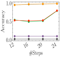
() Vary #steps: clustering

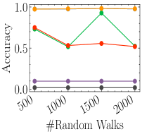
(a) Vary #walks: clustering

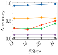
(b) Vary #steps: biclustering

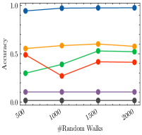
(c) Vary #walks: biclustering

Figure 1: Accuracies of the algorithms on WikiS. We consider clustering (Figs. 1() and 1(a)) and biclustering (Figs. 1(b) and 1(c)) experiments, with varying number of steps (Figs. 1() and 1(b)) and varying number of random walks (Figs. 1(a) and 1(c)). Since FOCG and polarSeeds do not use the number of steps and random walks as input, we only ran them once.

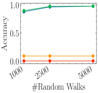
() WikiL: clustering

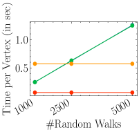
(a) WikiL: avg. query time

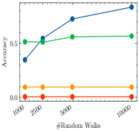
(b) WikiM: biclustering

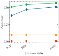
(c) WikiL: biclustering

Figure 2: Results on WikiM and WikiL for varying numbers of random walks. We present accuracies for clustering on WikiL (Fig. 2()), and for biclustering in WikiM (Fig. 2(b)) and in WikiL (Fig. 2(c)). The running time per vertex for clustering in WikiL is given in Fig. 2(a). Since FOCG and polarSeeds do not use random walks as input, we only ran them once.

Experiments on WikiS. Fig. 1 shows our results on WikiS. Unless stated otherwise, our oracles used $1000$ random walks of length $20$. For clustering (biclustering) experiments, the seeded oracles obtained $10$ ($5$) seeds for each $U_{i}$ ($V_{i}$); the unseeded oracles sampled $5k$ vertices, where $k=5$ for clustering and $k=10$ for biclustering. For the clustering experiments (Figs. 1() and 1(a)), the seeded oracles achieve almost perfect accuracy; the unseeded methods are worse and benefit from longer random walks (Fig. 1()). For the biclustering experiments (Figs. 1(b) and 1(c)), rw-seeded is by far the best method and achieves excellent accuracies. rw-u-seeded consistently achieves accuracies above 50% but below 60%; this suggests that rw-u-seeded successfully finds the clusters $U_{i}$ (as shown by the clustering results) but, as it ignores the edge signs, it places the vertices into the biclusters $V_{2i-1}$ and $V_{2i}$ only slightly better than random. For biclustering, the unseeded methods do not perform well. FOCG and polarSeeds achieve low accuracies, since they return too small clusters.

Experiments on WikiM and WikiL. Fig. 2 presents our results on the larger datasets. We did not run the unseeded oracles, since in WikiM and WikiL not all vertices are contained in ground-truth communities. We used random walks of length $24$ for WikiM and of length $20$ for WikiL; we initialized the seeds as for WikiS. Fig. 2() shows that even on WikiL, the seeded oracles find the clusters $U_{i}$ with almost perfect accuracy. Furthermore, the algorithms scale linearly in the number of random walks and on average queries takes less than 1.4 seconds (Fig. 2(a)). However, compared to WikiS, we obtain lower accuracies for the biclustering experiments: while on WikiM, rw-seeded still achieves accuracies over 83% with enough random walks (Fig. 2(b)), for WikiL even with 10 000 random walks, rw-seeded only achieves an accuracy of 50% (Fig. 2(c)). We blame this on the fact that in WikiL the ground-truth clusters are relatively small (they contain only 3.7% of the vertices). Additionally, in WikiL the fraction of negative edges is only 8%, and thus only few random walks will encounter a negative edge and rw-seeded cannot benefit from the edge-sign information. As before, FOCG and polarSeeds have low accuracies.

Conclusion. Our oracles are successful for finding polarized communities $U_{i}$, even when the graphs do not have bounded degrees (as in our theoretical analysis). rw-seeded is successful in finding the biclusters $(V_{2i-1},V_{2i})$, as long as they are large enough and there are enough negative edges.

5 Conclusion

We presented a local clustering oracle for signed graphs. Given a vertex $u$, the oracle can return the cluster membership of $u$ in sublinear time. Such a data structure is desirable when the input graphs are large and the cluster membership is only required for a small number of vertices. We proved that if the graph satisfies a clusterability assumption, then the oracle returns correct cluster memberships for a $(1-\epsilon)$-fraction of the vertices w.r.t. a hidden set of ground-truth clusters. We also evaluated the oracle practically, showing that it achieves good results for large clusters.

In the future it will be interesting to provide a theoretical analysis for our biclustering heuristic; here, ideas from Trevisan (2012) might be helpful. From a practical point of view it would be interesting to obtain improvements for our biclustering heuristic, which allow to find small biclusters $(V_{2i-1},V_{2i})$ when there are few negative edges. Two directions for this might be as follows: (1) For a node $u$, first identify the cluster $U_{i}$ of $u$ using the unsigned oracle and then use auxiliary information to decide whether $u$ belongs to $V_{2i-1}$ or to $V_{2i}$. (2) When the underlying graph contains few negative edges, bias the random walks of rw-seeded such that it takes disproportionately many negative edges.

Appendix A Overview of the Appendix

The appendix is organized as follows:

• Appendix B: We provide further motivation for our choice of the inner signed bipartiteness ratio.

• Appendix C: We present the pseudocode for our algorithms.

• Appendix D: We give an overview of our proof strategy.

• Appendix E: We present the full proofs for all claims in the main text.

• Appendix F: We give details on the implementations of our algorithms, including parameter tuning.

• Appendix G: We evaluate our algorithm on synthetically generated data.

Appendix B Further Motivation of the Inner Signed Bipartiteness Ratio

We provide further motivation for the inner signed bipartiteness ratio. Recall that we set

$$\beta^{\text{inner}}(G):=\min_{\emptyset\neq U\subseteq V\colon\operatorname{vol}(U)\leq\frac{1}{2}\operatorname{vol}(G)}\beta_{G}(U).$$

First, let us justify our intuition that if $\beta^{\text{inner}}(G)$ is large, then $\beta^{\text{inner}}(G)$ cannot be decomposed into two nearly-balanced communities. To make this more formal, recall the definition of $\beta_{2}(G)=\min_{U_{1},U_{2}}\max_{i=1,2}\beta_{G}(U_{i})$, where the minimum is taken over all partitions $U_{1},U_{2}$ of $V$ with $U_{1},U_{2}\neq\emptyset$. Now note that if we could split $G$ into two nearly-balanced communities, then we would have that $\beta_{2}(G)$ is small. Thus, we show that if $\beta^{\text{inner}}(G)$ is large then $\beta_{2}(G)$ is at least as large. This justifies our informal intuition above.

Lemma 7.

It holds that $\beta_{2}(G)\geq\beta^{\text{inner}}(G)$. In particular, if $\beta_{\text{in}}\in\mathbb{R}_{\geq 0}$ and $\beta^{\text{inner}}(G)\geq\beta_{\text{in}}$ then $\beta_{2}(G)\geq\beta_{\text{in}}$.

Proof.

We prove the first claim by contradiction, i.e., suppose that $\beta^{\text{inner}}(G)=\beta_{\text{in}}$ and $\beta_{2}(G)<\beta_{\text{in}}=\beta^{\text{inner}}(G)$. Then there exists a partition $U_{1},U_{2}$ of $V$ such that $\beta_{G}(U_{1})<\beta_{\text{in}}$ and $\beta_{G}(U_{2})<\beta_{\text{in}}$. Next, since $U_{1}$ and $U_{2}$ form a partition of $V$, we must have that $\operatorname{vol}(U_{1})\leq\frac{1}{2}\operatorname{vol}(G)$ or $\operatorname{vol}(U_{2})\leq\frac{1}{2}\operatorname{vol}(G)$. This implies that there exists a set $U\in\{U_{1},U_{2}\}$ such that $\operatorname{vol}(U)\leq\frac{1}{2}\operatorname{vol}(G)$ and $\beta_{G}(U)<\beta_{\text{in}}$. Thus, $\beta^{\text{inner}}(G)<\beta_{\text{in}}$. But this contradicts our assumption that $\beta^{\text{inner}}(G)=\beta_{\text{in}}$.

The second claim of the lemma immediately follows from applying the first claim. ∎

Why do we not assume that $\beta(G[U_{i}])$ is large? Next, we discuss why we cannot replace the inner signed bipartiteness ratio $\beta^{\text{inner}}(G)$ with the (classic) signed bipartiteness ratio $\beta(G[U_{i}])$ in Def. 3. To see this, consider Def. 3 with $\beta^{\text{inner}}(G[U_{i}])\geq\beta_{\text{in}}$ replaced by $\beta(G[U_{i}])\geq\beta_{\text{in}}$ for all $i=1,\dots,k$. Again, we consider the the setting with $\beta_{\text{in}}>\beta_{\text{out}}$. Intuitively, this would mean that subgraph $G[U_{i}]$ is “far from balanced” on its inside (since $\beta(G[U_{i}])$ is large) while outside it is close to balanced (since $\beta_{G}(U_{i})$ is small).

Unfortunately, we show that if $\beta_{\text{in}}>\beta_{\text{out}}$ then no graph can satisfy this new definition. Before we give a more general proof, consider the following example. Consider a graph $G$ which consists of two positive cliques among vertices $V_{1}$ and $V_{2}$ and in between $V_{1}$ and $V_{2}$ there is biclique consisting only of negative edges. Then $\beta(G)=0$ and $\beta(V_{1},V_{2})=0$ but also $\beta(G[V_{1}])=0$ and $\beta(G[V_{2}])=0$ (since graphs with only positive edges are balanced).

Now we give a more general result showing that for any $U\subseteq V$, we have that $\beta(G[U])\leq\beta_{G}(U)$. Therefore, the previously proposed definition that avoids the inner signed bipartiteness ratio cannot work: it implies that $\beta_{\text{in}}\leq\beta(G[U_{i}])\leq\beta_{G}(U_{i})\leq\beta_{\text{out}}$ but this contradicts our assumption that $\beta_{\text{in}}>\beta_{\text{out}}$.

Lemma 8.

For any two disjoint subsets $V_{1},V_{2}\subseteq V$, it holds that $\beta(G[V_{1}\cup V_{2}])\leq\beta_{G}(V_{1},V_{2})$. Furthermore, for any $U\subseteq V$, it holds that $\beta(G[U])\leq\beta_{G}(U)$.

Proof.

We have that

$$\beta(G[V_{1}\cup V_{2}])$$

$$\leq\beta_{G[V_{1}\cup V_{2}]}(V_{1},V_{2})$$

$$=\frac{2\left|E_{G}^{+}(V_{1},V_{2})\right|+\left|E_{G}^{-}(V_{1})\right|+\left|E_{G}^{-}(V_{2})\right|}{\operatorname{vol}_{G[V_{1}\cup V_{2}]}(V_{1},V_{2})}$$

$$\leq\frac{2\left|E_{G}^{+}(V_{1},V_{2})\right|+\left|E_{G}^{-}(V_{1})\right|+\left|E_{G}^{-}(V_{2})\right|+\left|E_{G}(V_{1}\cup V_{2},\overline{V_{1}\cup V_{2}})\right|}{\operatorname{vol}_{G[V_{1}\cup V_{2}]}(V_{1},V_{2})+\left|E_{G}(V_{1}\cup V_{2},\overline{V_{1}\cup V_{2}})\right|}$$

$$=\beta_{G}(V_{1},V_{2}),$$

where we have used that for $a,b,c>0$ and $a\leq b$, it holds that $\frac{a}{b}\leq\frac{a+c}{b+c}$.

Now for any subset $U$, let $V_{1},V_{2}$ be a partition of $U$ such that $\beta_{G}(U)=\beta_{G}(V_{1},V_{2})$. Then by the above calculation, we have that

$$\beta(G[U])\leq\beta_{G[U]}(V_{1},V_{2})\leq\beta_{G}(V_{1},V_{2})=\beta_{G}(U).\qed$$

Is the underlying unsigned graph clusterable? Next, we argue that our condition from Def. 3 is not implied by previous definitions that were based on the conductance of unsigned graphs (e.g., in Czumaj et al. (2015)). In other words, it is possible that our methods finds the planted clusters in the signed graph while this would not be possible by only looking at the underlying unsigned graph.

First, recall that for an unsigned graph $G^{\textrm{un}}=(V,E)$ and a set of vertices $S\subseteq V$, the conductance of $S$ is given by $\phi_{G^{\textrm{un}}}(S)=\frac{\left|E(S,V\setminus S)\right|}{\operatorname{vol}(S)}$. Furthermore, we let $\phi(G^{\textrm{un}})$ denote the conductance of $G^{\textrm{un}}$ which is given by $\phi(G^{\textrm{un}})=\min\{\phi_{G^{\textrm{un}}}(S)\colon\operatorname{vol}(S)\leq\operatorname{vol}(G^{\textrm{un}})/2\}$.

Now consider the unsigned graph $G^{\textrm{un}}$ that is obtained by removing all the signs on the edges from $G$. We argue that a $(k,\beta_{\text{in}},\beta_{\text{out}})$-clustering of $G$ does not imply a $(k,\beta_{\text{in}},\beta_{\text{out}})$-clustering of $G^{\textrm{un}}$, i.e., $G^{\textrm{un}}$ contains a $k$-partition $C_{1},\dots,C_{k}$ such that the inner conductance of $C_{i}$, denoted $\phi(G^{\textrm{un}}[C_{i}])$, is at least $\beta_{\text{in}}$ and the outer conductance of $C_{i}$, denoted $\phi_{G}(C_{i})$, is at most $\beta_{\text{out}}$ for each $i$. Therefore, one could not apply the previous clustering oracle for conductance-based clustering of $G^{\textrm{un}}$ and recover the underlying clusters in our problem. We give a brief explanation next.

Suppose that $U_{1},\dots,U_{k}$ is a $(k,\beta_{\text{in}},\beta_{\text{out}})$-clustering of $G$. Then, indeed, it is true that each $U_{i}$ has small outer conductance in $G^{\textrm{un}}$, since we have that $\phi_{G^{\textrm{un}}}(U_{i})\leq\beta_{G}(U_{i})\leq\beta_{\text{out}}$. However, the inner conductance of $U_{i}$ in $G^{\textrm{un}}$ can be arbitrarily small: Even though the inner signed bipartiteness ratio of $U_{i}$ is large, it can happen that there is a very small subset $S_{i}\subseteq U_{i}$ (say, of size $O(\log n)$) such that there are almost no edges leaving $S_{i}$ but all edges in $S_{i}$ have sign $-$ and $S_{i}$ is far from being balanced. Thus, there exists a subset $S_{i}$ in $U_{i}$ whose (outer) conductance is almost $0$ in $G^{\textrm{un}}$ but the inner signed bipartiteness ratio of $S_{i}$ and $U_{i}$ is large.

Note that the previous example with the set $S_{i}$ also shows that it is possible that $G$ contains a sparse cut and, therefore, $\mathbf{p}_{u}^{t}$ does not converge to the uniform distribution of $V$.

Appendix C Pseudocode for Our Algorithms

Algorithm 1 Estimating the dot product $\langle\mathbf{p}_{u}^{t}\mathbf{D}^{-1/2},\mathbf{p}_{v}^{t}\mathbf{D}^{-1/2}\rangle$

1:procedure EstDotProd($u,v,t,\alpha$)

2:     $R\leftarrow\frac{40000d^{2}k^{1.5}\sqrt{n}}{\alpha^{1.5}}$

3:     for all $i=1,\cdots,h=O(\log n)$ do

4:         for $x\in\{u,v\}$ do

5:              Perform $R$ lazy signed random walks of length $t$ starting at vertex $x$ with sign $+$.

6:              for each $w\in V$ do

7:                  $\mathbf{m}^{+}_{x}(w)\leftarrow$ the fraction of walks that end at $w$ with sign $+$.

8:                  $\mathbf{m}^{-}_{x}(w)\leftarrow$ the fraction of walks that end at $w$ with sign $-$.

9:                   $\mathbf{m}_{x}\leftarrow(\mathbf{m}_{x}^{+}-\mathbf{m}_{x}^{-})\mathbf{D}^{-1/2}$.                        

10:         $\chi_{i}\leftarrow\langle\mathbf{m}_{u},\mathbf{m}_{v}\rangle$.      

11:     Let $X_{uv}$ be the median value of $\chi_{1},\cdots,\chi_{h}$.

12:     return $X_{uv}$

Algorithm 2 Preprocessing: Constructing a clustering oracle

1:procedure BuildOracle($G,k,d,\beta_{\text{in}},\epsilon,\gamma$)

2:     $s\leftarrow\frac{20k\log({k})}{\gamma}$, $\alpha\leftarrow\frac{\epsilon}{90s}$, $t\leftarrow\frac{C^{\prime\prime}k^{6}d^{3}\log n}{\epsilon\cdot\beta_{\text{in}}^{2}}$ for constant $C^{\prime\prime}$

3:     Sample a set $S$ of $s$ vertices independently and uniformly at random from $V$.

4:     for $v\in S$ do $\triangleright$ test if $||\mathbf{p}_{v}^{t}\mathbf{D}^{-1/2}||_{2}^{2}=O(\frac{k^{2}\log(k)}{\gamma\epsilon\cdot n})$

5:         $X_{vv}\leftarrow$EstDotProd($v,v,t,\alpha$)

6:         if $X_{vv}\geq\frac{4000k^{2}\log(k)}{\gamma\epsilon\cdot n}$ then

7:               abort and return Fail               

8:     let $H$ be an empty graph with vertex set $S$

9:     for each pair $u,v\in S$ do $\triangleright$ test if $\Delta_{uv}\leq\frac{1}{4nd}$

10:         $X_{vv}\leftarrow$EstDotProd($v,v,t,\alpha$)

11:         $X_{uu}\leftarrow$EstDotProd($u,u,t,\alpha$)

12:         $X_{uv}\leftarrow$EstDotProd($u,v,t,\alpha$)

13:          $\delta_{uv}\leftarrow\min\{X_{vv}+X_{uu}-2X_{uv},X_{vv}+X_{uu}+2X_{uv}\}$

14:         if $\delta_{uv}\leq\frac{1}{2dn}$ then

15:               add edge $(u,v)$ to $H$               

16:     if $H$ is the union of $k$ connected components (CCs) then

17:         label the components by “$1,2,\dots,k$’

18:         label each vertex $u\in V_{H}$ with the same index as its component, denoted $\ell(u)$

19:         return $H$ and its vertex labeling $\ell$

20:     else

21:         return Fail      

Algorithm 3 Answering the community membership of a vertex $v$

1:procedure WhichCluster($G,v,H,\ell$)

2:     for $u\in V_{H}$ do

3:         $X_{vv}\leftarrow$EstDotProd($v,v,t,\alpha$)

4:         $X_{uu}\leftarrow$EstDotProd($u,u,t,\alpha$)

5:         $X_{uv}\leftarrow$EstDotProd($u,v,t,\alpha$)

6:          $\delta_{uv}\leftarrow\min\{X_{vv}+X_{uu}-2X_{uv},X_{vv}+X_{uu}+2X_{uv}\}$

7:         if $\delta_{uv}\leq\frac{1}{2dn}$ then

8:              abort and return the label $\ell(u)$               

9:     return a random number from $\{1,2,\dots,k\}$

Appendix D Analysis Overview

In this section, we give an overview of the analysis and provide the main technical lemmas of our analysis. All missing proofs can be found in App. E.

Intuition. We begin by providing some intuition for our algorithm and our analysis.

We start by establishing some properties of lazy signed random walks. First, suppose that we perform the lazy random walks without the signs on the underlying unsigned graph $G^{\textrm{un}}$ with the corresponding transition probability matrix $\mathbf{W}^{\textrm{un}}:=\frac{\mathbf{I}+\mathbf{D}^{-1}\mathbf{A}^{\textrm{un}}}{2}$, where $\mathbf{A}^{\textrm{un}}$ is the adjacency matrix of $G^{\textrm{un}}$. Then the probability that a random walk started at vertex $u$ ends in vertex $v$ is $\mathbf{Pr}\left(v_{t}=v\right)=\mathbf{q}_{u}^{t}(v)$, where $\mathbf{q}_{u}^{t}=\mathbf{1}_{u}(\mathbf{W}^{\textrm{un}})^{t}$. Second, when we add the sign, then we are interested in the quantity

$$\mathbf{p}_{u}^{t}(v)=\mathbf{Pr}\left(v_{t}=v,s_{t}=+\right)-\mathbf{Pr}\left(v_{t}=v,s_{t}=-\right),$$

i.e., $\mathbf{p}_{u}^{t}(v)$ is the probability of reaching $v$ with a positive sign minus the probability of reaching $v$ with a negative sign. Observe that $\mathbf{p}_{u}^{t}(v)$ can be described by the walk matrix $\mathbf{W}=\frac{\mathbf{I}+\mathbf{D}^{-1}\mathbf{A}^{\sigma}}{2}$, i.e., $\mathbf{p}_{u}^{t}(v)=[\mathbf{1}_{u}\mathbf{W}^{t}](v)$ for all $v$. Note that while $\mathbf{q}_{u}^{t}$ (for unsigned random walks) gives a distribution, this is not the case for $\mathbf{p}_{u}^{t}$. In fact, $\mathbf{p}_{u}^{t}$ can potentially even contain negative entries and $\mathbf{p}_{u}^{t}$ does not necessarily converge to the uniform distribution of $V$ as it can happen that $V$ contains a sparse cut (we discuss this in App. B). In the following, we call such a vector $\mathbf{p}_{u}^{t}$ the discrepancy vector of a lazy signed random walk of length $t$ starting from $u$.

Next, consider a signed graph $G$ and a $(k,\beta_{\text{in}},\beta_{\text{out}})$-clustering $U_{1},\dots,U_{k}$ of $G$ as per Def. 3. Let $U\in\{U_{1},\dots,U_{k}\}$ be one of the clusters. Since by assumption we have that $\beta_{G}(U)\leq\beta_{\text{out}}$, there exists a partition of $U$ into subsets $V_{1}$ and $V_{2}$ with $\beta_{G}(V_{1},V_{2})\leq\beta_{\text{out}}$. Then, intuitively, for a typical vertex $u\in U$, a short random walk starting from $u$ of has the following properties:

1. Since the walk is short (this is crucial), the walk will be “trapped” in $U$, as there are only few edges leaving $U$. Thus, for the discrepancy vector it should hold that $\sum_{v\in U}\left|\mathbf{p}_{u}^{t}(v)\right|\gg\sum_{v\in V\setminus U}\left|\mathbf{p}_{u}^{t}(v)\right|$.

2. If $u\in V_{1}$ then most walks ending at vertices $v\in V_{1}$ should have a positive sign and most walks ending at vertices $V\in V_{2}$ should have negative sign. Thus, for the discrepancy vector $\mathbf{p}_{u}^{t}$ it should hold that $\mathbf{p}_{u}^{t}(v)>0$ if $v\in V_{1}$ and $\mathbf{p}_{u}^{t}(v)<0$ if $v\in V_{2}$. Similarly, if $u\in V_{2}$ then the same holds with flipped signs.

3. Let $u\in U$. If two vertices $x,y$ are from the same sub-communities (i.e., $x,y\in V_{1}$ or $x,y\in V_{2}$), then $\mathbf{p}_{u}^{t}(x)\approx\mathbf{p}_{u}^{t}(y)$, i.e., the discrepancy on $x$ is close to the discrepancy on $y$.

Now let us discuss how we can use the discrepancy vectors $\mathbf{p}_{u}^{t}$ and $\mathbf{p}_{v}^{t}$ to decide whether $u$ and $v$ are in the same cluster or not. Our goal is to find a distance function $\Delta_{uv}=\Delta_{uv}(\mathbf{p}_{u}^{t},\mathbf{p}_{v}^{t})$ such that $\Delta_{uv}$ is small iff $u$ and $v$ are from the same cluster $U$.

First, consider vertices $u\in U_{i}$ and $v\in U_{j}$, $i\neq j$, from different clusters. Then Property (i) suggests that $\mathbf{p}_{u}^{t}$ and $\mathbf{p}_{v}^{t}$ have most of their mass in different entries and thus $\lVert\mathbf{p}_{u}^{t}-\mathbf{p}_{v}^{t}\rVert_{2}^{2}$ should be large.

Second, consider vertices $u,v\in U$ from the same cluster. Let $U=V_{1}\cup V_{2}$ as above. If $u,v\in V_{1}$ or $u,v\in V_{2}$ then the properties above suggest $\mathbf{p}_{u}^{t}\approx\mathbf{p}_{v}^{t}$ and thus $\lVert\mathbf{p}_{u}^{t}-\mathbf{p}_{v}^{t}\rVert_{2}^{2}\approx 0$ is small. However, if $u\in V_{1}$ and $v\in V_{2}$, then $\mathbf{p}_{u}^{t}\approx-\mathbf{p}_{v}^{t}$ by Property (ii) and (iii) and thus $\lVert\mathbf{p}_{u}^{t}-\mathbf{p}_{v}^{t}\rVert_{2}^{2}\approx\lVert 2\mathbf{p}_{u}^{t}\rVert_{2}^{2}$ will still be large. However, this issue can be mitigated if we use $\mathbf{r}_{u}^{t}=\left|\mathbf{p}_{u}^{t}\right|$ and $\mathbf{r}_{v}^{t}=\left|\mathbf{p}_{v}^{t}\right|$ instead of $\mathbf{p}_{u}^{t}$ and $\mathbf{p}_{v}^{t}$. Here, the absolute values are applied component-wise, i.e., $\mathbf{r}_{u}^{t}(v)=\left|\mathbf{p}_{u}^{t}(v)\right|$ for all $v$.

Therefore, in our analysis we would like to use $\lVert\mathbf{r}_{u}^{t}-\mathbf{r}_{v}^{t}\rVert^{2}_{2}$ as a distance measure. However, due to some technical difficulties in the analysis of this quantity, we cannot use the vectors $\mathbf{r}_{u}^{t}$ and instead we consider $\min\{\lVert\mathbf{p}_{u}^{t}-\mathbf{p}_{v}^{t}\rVert^{2}_{2},\lVert\mathbf{p}_{u}^{t}+\mathbf{p}_{v}^{t}\rVert^{2}_{2}\}$ which behaves similar to taking the absolute values and also fixes the issue with Property (ii). After adding some degree corrections, we arrive at our final distance measure $\Delta_{uv}=\min\{\lVert\mathbf{p}_{u}^{t}\mathbf{D}^{-1/2}-\mathbf{p}_{v}^{t}\mathbf{D}^{-1/2}\rVert^{2}_{2},\lVert\mathbf{p}_{u}^{t}\mathbf{D}^{-1/2}+\mathbf{p}_{v}^{t}\mathbf{D}^{-1/2}\rVert^{2}_{2}\}$. Note that $\Delta$ is a pseudometric distance, i.e., one may have that $\Delta_{uv}=0$ for distinct vectors $\mathbf{p}_{u}^{t}$ and $\mathbf{p}_{v}^{t}$.

D.1 Main Technical Lemmas

We give a technical overview of our analysis. Note that while our high-level proof strategy is relatively similar to the one used in Czumaj et al. (2015) for unsigned graphs, the concrete proofs are often quite different. It required a substantial amount of work and new ideas to obtain our results for signed graphs.

Random walks from the same cluster. First, we show that if $U$ is a polarized community with large inner signed bipartiteness ratio and small (outer) bipartiteness ratio, then for most of the vertices $u,v\in U$ their distance $\Delta_{uv}$ is small.

Lemma 9.

Let $\alpha,\gamma\in(0,1)$. Let $G=(V,E,\sigma)$ be a signed, $d$-bounded degree, $(k,\beta_{\text{in}},\beta_{\text{out}})$-clusterable graph. Let $U$ be a subset of $V$ such that $\left|U\right|\geq\gamma n$, $\beta^{\text{inner}}(G[U])\geq\beta_{\text{in}}$ and $\beta_{G}(U)\leq\beta_{\text{out}}$. Then for all $t\geq\frac{4C_{1}^{2}(k+1)^{6}\log n}{\beta_{\text{in}}^{2}}$, $\beta_{\text{out}}<\alpha_{1}\beta_{\text{in}}^{2}$ where $\alpha_{1}=\frac{\alpha\gamma}{800000C_{1}^{2}kd^{3}}$, there exists a subset $\widetilde{U}\subseteq U$ with $\left|\widetilde{U}\right|\geq(1-\alpha)\left|U\right|$ and for all $u,v\in\widetilde{U}$, it holds that $\Delta_{uv}\leq\frac{1}{4nd}$.

Proving Lem. 9 was one of the main obstacles for obtaining our results. We will give an overview of its proof and our main technical contribution in Sec. 3.2.

Random walks from two different clusters. We further show that if we have two disjoint communities $U_{1}$ and $U_{2}$, then for most vertices $u\in U_{1}$ and $v\in U_{2}$ their distance $\Delta_{uv}$ must be large. Note that while Lem. 9 assumes a lower bound on the walk length $t$, Lem. 10 assumes an upper bound on $t$. Thus, it is crucial that the random walks have the correct length $\Theta(\log n)$.

Lemma 10.

Let $U_{1}$ and $U_{2}$ be two disjoint subsets with $\beta_{G}(U_{1}),\beta_{G}(U_{2})\leq\beta_{\text{out}}$. Let $0<\alpha<1$. For any $0\leq t\leq\frac{\alpha}{8\beta_{\text{out}}}$, there exist subsets $\widehat{U_{1}}\subseteq U_{1},\widehat{U_{2}}\subseteq U_{2}$ such that $|\widehat{U_{1}}|\geq(1-\alpha)|U_{1}|$, $|\widehat{U_{2}}|\geq(1-\alpha)|U_{2}|$, and for any $u\in\widehat{U_{1}}$ and $v\in\widehat{U_{2}}$, it holds that $\Delta_{uv}\geq\frac{1}{nd}$.

$\ell_{2}^{2}$-norm of the vector $\mathbf{p}_{v}^{t}\mathbf{D}^{-1/2}$. Based on the previous two lemmas, our goal will be to test whether $\Delta_{uv}\leq\frac{1}{4nd}$ or $\Delta_{uv}\geq\frac{1}{nd}$. To this end, we wish to use EstDotProd to approximate $\Delta_{uv}$ via Eqn.s (2) and (3). To prove this, we first give a useful bound on the $\ell_{2}^{2}$-norm of the vectors $\mathbf{p}_{v}^{t}\mathbf{D}^{-1/2}$.

Lemma 11.

Let $\alpha\in(0,1)$. Suppose $G=(V,E,\sigma)$ is a signed and $(k,\beta_{\text{in}},\beta_{\text{out}})$-clusterable graph. Then there exists a set $V^{\prime}\subseteq V$ of size $\left|V^{\prime}\right|\geq(1-\alpha)\left|V\right|$ such that for all $u\in V^{\prime}$ and all $t\geq\frac{C_{1}^{2}(k+1)^{6}\log n}{\beta_{\text{in}}^{2}}$, we have that $\lVert\mathbf{p}_{v}^{t}\mathbf{D}^{-1/2}\rVert^{2}_{2}\leq\frac{2k}{\alpha n}$.

Estimating the dot product. Now we prove that EstDotProd($u$,$v$,$t$,$\alpha$) estimates $\langle\mathbf{p}_{u}^{t}\mathbf{D}^{-1/2},\mathbf{p}_{v}^{t}\mathbf{D}^{-1/2}\rangle$ with small error.

Lemma 12.

Let $\alpha\in(0,1)$ be a number such that $\frac{2k}{\alpha}\leq n$. Suppose $G=(V,E,\sigma)$ is a signed and $(k,\beta_{\text{in}},\beta_{\text{out}})$-clusterable graph. Let $t\geq\frac{C_{1}^{2}(k+1)^{6}\log n}{\beta_{\text{in}}^{2}}$. Let $V^{\prime}\subseteq V$ be the set of vertices satisfying the property given by Lem. 11. Then EstDotProd($u,v,t,\alpha$) outputs $X_{uv}$ such that with probability $1-1/n^{3}$, it holds that

$$\left|X_{uv}-\langle\mathbf{p}_{v}^{t}\mathbf{D}^{-1/2},\mathbf{p}_{u}^{t}\mathbf{D}^{-1/2}\rangle\right|\leq\frac{1}{20nd}$$

for all $u,v\in V^{\prime}$. Furthermore, EstDotProd($u,v,t,\alpha$) runs in time $O(\frac{d^{2}k^{1.5}t\log n}{\alpha^{1.5}}\cdot\sqrt{n})$.

To prove Thm. 4, we first show that an overwhelming fraction of the vertices are “well-behaved” in the senses of Lem.s 9–11. Then, if we only consider these “well-behaved” vertices, we can apply Lem. 12 and this will classify all of these vertices correctly with high probability.

Appendix E Deferred Proofs

E.1 Proof of Lemma 5

Now we prove Lem. 5, which is restated in the following for the sake of readability. See 5

Proof of Lemma 5.

Since $G$ is $(k,\beta_{\text{in}},\beta_{\text{out}})$-clusterable, there exists a partition of $V$ into clusters $(C_{1},\dots,C_{k})$ such that $\beta^{\text{inner}}(G[C_{i}])\geq\beta_{\text{in}}$ and $\beta_{G}(C_{i})\leq\beta_{\text{out}}$ for all $i\in[k]$. Therefore, $\beta_{k}(G)\leq\max_{i}\beta_{G}(C_{i})\leq\beta_{\text{out}}$. Now Thm. 2 implies that $\lambda_{k}\leq 2\beta_{k}(G)\leq 2\beta_{\text{out}}$. Thus, $\lambda_{1}\leq\cdots\leq\lambda_{k}\leq 2\beta_{\text{out}}$.

The next part shows that $\lambda_{k+1}\geq\frac{\beta_{\text{in}}^{2}}{C_{1}^{2}(k+1)^{6}}$. Consider any $k+1$ disjoint subsets $V_{1},\dots,V_{k+1}$.

Now observe that there must exist a subset $V_{i_{0}}\in\{V_{1},\dots,V_{k+1}\}$ with following property: for all $i\in[k]$, $\operatorname{vol}(V_{i_{0}}\cap C_{i})\leq\frac{1}{2}\operatorname{vol}(C_{i})$. To see that this is the case, suppose that the statement is false, i.e., no such subset exists. Then by pigeonhole principle there must exist indices $j_{1}$, $j_{2}$ with $j_{1}\neq j_{2}$ and index $j_{3}$ such that $V_{j_{1}}\cap C_{j_{3}}$ and $V_{j_{2}}\cap C_{j_{3}}$ have volume more than $\frac{1}{2}\operatorname{vol}(C_{j_{3}})$. This is a contradiction since the sets $V_{j_{1}}$ and $V_{j_{2}}$ are mutually disjoint.

For the rest of the proof, consider the subset $V_{i_{0}}$ with the above property. Consider an arbitrary partition $L,R$ of $V_{i_{0}}$, such that $L\cup R=V_{i_{0}}$ and $L\cap R=\emptyset$. Let $L_{i}=C_{i}\cap L$ and $R_{i}=C_{i}\cap R$. Observe that $V_{i_{0}}=\bigcup_{i}(L_{i}\cup R_{i})$ since $V=\bigcup_{i}C_{i}$. Since $\beta^{\text{inner}}(G[C_{i}])\geq\beta_{\text{in}}$ and $\operatorname{vol}(L_{i}\cup R_{i})\leq\frac{1}{2}\operatorname{vol}(C_{i})$ for all $i\leq k$, we get that $\beta_{G[C_{i}]}(L_{i}\cup R_{i})\geq\beta_{\text{in}}$ for all $i\in[k]$. In particular, this implies that $\beta_{G[C_{i}]}(L_{i},R_{i})=\frac{e_{G[C_{i}]}(L_{i},R_{i})}{\operatorname{vol}(L_{i}\cup R_{i})}\geq\beta_{\text{in}}$ for all $i\in[k]$. Thus,

$$\beta_{G}(L,R) =\frac{e_{G}(L,R)}{\operatorname{vol}(L\cup R)}$$

$$=\frac{2\left|E^{+}_{G}(L,R)\right|+\left|E^{-}_{G}(L)\right|+\left|E^{-}_{G}(R)\right|+\left|E_{G}(L\cup R,V\setminus(L\cup R))\right|}{\operatorname{vol}(L\cup R)}$$

$$\geq\frac{1}{\operatorname{vol}(L\cup R)}\sum_{i\in[k]}\Big{[}2\left|E^{+}_{G}(L_{i},R_{i})\right|+\left|E^{-}_{G}(L_{i})\right|+\left|E^{-}_{G}(R_{i})\right|+\left|E_{G}(L_{i}\cup R_{i},C_{i}\setminus(L_{i}\cup R_{i}))\right|\Big{]}$$

$$=\frac{\sum_{i\in[k]}e_{G[C_{i}]}(L_{i},R_{i})}{\sum_{i\in[k]}\operatorname{vol}(L_{i}\cup R_{i})}$$

$$\geq\frac{\sum_{i\in[k]}\beta_{\text{in}}\operatorname{vol}(L_{i}\cup R_{i})}{\sum_{i\in[k]}\operatorname{vol}(L_{i}\cup R_{i})}$$

$$\geq\beta_{\text{in}}.$$

Since $L,R$ is an arbitrary partition of $V_{i_{0}}$, it holds that $\beta_{G}(V_{i_{0}})\geq\beta_{\text{in}}$. Thus, $\beta_{k+1}(G)\geq\beta_{\text{in}}$. Now Thm. 2 implies that $\lambda_{k+1}\geq\frac{\beta_{\text{in}}^{2}}{C_{1}^{2}(k+1)^{6}}$. ∎

E.2 Proof of Lemma 6

Now we prove Lem. 6, which is restated in the following for the sake of readability. See 6

Proof.

The proof is based on the following intuition. Recall the definitions of vectors $\mathbf{v}^{\prime}_{i},\mathbf{1}_{V_{1},V_{2}},\mathbf{w}_{1}$ from the above discussion. Since both $\mathbf{v}^{\prime}_{i}$ and a scalar multiplications of $\mathbf{1}_{V_{1},V_{2}}$ have small total ‘discrepancy’ over the set of all edges (i.e., Ineq. (4) and (7)), and the ratio between the total ‘discrepancy’ over all the edges and the total ‘discrepancy’ over all vertices (w.r.t. some centers defined by $\mathbf{w}_{1}$) is large (i.e., Ineq. (8)), one can guarantee both that $\mathbf{v}_{i}^{\prime}$ and a scaled multiplication of $\mathbf{1}_{V_{1},V_{2}}$ are close to (another scalar multiplication of) $\mathbf{w}_{1}$. We now give the details.

Since $G$ is $(k,\beta_{\text{in}},\beta_{\text{out}})$-clusterable, we can apply Lem. 5 to obtain $\lambda_{k+1}\geq\frac{\beta_{\text{in}}^{2}}{C_{1}^{2}(k+1)^{6}}$ and $\lambda_{i}\leq 2\beta_{\text{out}}$ for all $i\in[k]$.

Since for any $i\leq k$, $\mathbf{v}_{i}\mathbf{\mathcal{L}}^{\sigma}=\lambda_{i}\mathbf{v}_{i}$, we have $\mathbf{v}_{i}\mathbf{D}^{-1/2}(\mathbf{D}-\mathbf{A}^{\sigma})\mathbf{D}^{-1/2}=\lambda_{i}\mathbf{v}_{i}$, and thus

$$\lambda_{i} =\mathbf{v}_{i}\mathbf{D}^{-1/2}(\mathbf{D}-\mathbf{A}^{\sigma})\mathbf{D}^{-1/2}\mathbf{v}_{i}^{\top}$$

$$=\mathbf{v}^{\prime}_{i}(\mathbf{D}-\mathbf{A}^{\sigma}){\mathbf{v}^{\prime}_{i}}^{\top}$$

$$=\sum_{(u,v)\in E}\left(\mathbf{v}^{\prime}_{i}(u)-\sigma(uv)\mathbf{v}^{\prime}_{i}(v)\right)^{2}.$$

Thus, for any $i\leq k$,

$$\sum_{(u,v)\in E}\left(\mathbf{v}^{\prime}_{i}(u)-\sigma(uv)\mathbf{v}^{\prime}_{i}(v)\right)^{2}\leq 2\beta_{\text{out}}.$$ (4)

Now consider the subgraph $H=G[U]$ induced by the subset $U$. Denote the set of vertices of $H$ as $V_{H}=U$ and the set of edges of $H$ as $E_{H}$. By assumption on $U$, $\beta^{\text{inner}}(H)\geq\beta_{\text{in}}$ and $\beta_{G}(V[H])\leq\beta_{\text{out}}$.

Let $\lambda_{1}(H),\lambda_{2}(H)$ be the first and second eigenvalues of the normalized Laplacian matrix $\mathbf{\mathcal{L}}_{H}^{\sigma}$ of $H$. Next, let $\mathbf{D}_{H}$ be the degree matrix of $H$ and let $\mathbf{A}_{H}^{\sigma}$ denote the signed adjacency matrix of $H$.

Now we consider a partition $(V_{1},V_{2})$ of $U$ such that $\beta_{G}(U)=\beta_{G}(V_{1},V_{2})\leq\beta_{\text{out}}$. Then it holds that $\beta(H)\leq\beta_{H}(V_{1},V_{2})\leq\beta_{G}(V_{1},V_{2})\leq\beta_{\text{out}}$. Therefore, by Thm. 2,

$$\lambda_{1}(H)\leq 2\beta_{\text{out}}.$$

Let $\mathbf{1}_{V_{1},V_{2}}\in\mathbb{R}^{V_{H}}$ such that $\mathbf{1}_{V_{1},V_{2}}(u)=1$ if $u\in V_{1}$ and $-1$ otherwise. Set $\mathbf{b}:=\frac{\mathbf{1}_{V_{1},V_{2}}}{\sqrt{\mu_{U}}}$. Then it holds that

$$\sum_{(u,v)\in E}(\mathbf{b}(u)-\sigma(uv)\mathbf{b}(v))^{2} =\frac{\mathbf{1}_{V_{1},V_{2}}}{\sqrt{\mu_{U}}}(\mathbf{D}_{H}-\mathbf{A}_{H}^{\sigma})\frac{\mathbf{1}_{V_{1},V_{2}}\top}{\sqrt{\mu_{U}}}$$

$$=\frac{1}{\mu_{U}}\sum_{(u,v)\in E(H)}(\mathbf{1}_{V_{1},V_{2}}(u)-\sigma(u,v)\mathbf{1}_{V_{1},V_{2}}(v))^{2}$$

$$=\frac{2|E^{+}(V_{1},V_{2})|+|E^{-}(V_{1})|+|E^{-}(V_{2})|}{\mu_{U}}$$ (5)

$$=\beta_{H}(V_{1},V_{2})$$ (6)

$$\leq\beta_{\text{out}}.$$ (7)

Let $\mathbf{w}_{1}\in\mathbb{R}^{V_{H}}$ be an eigenvector corresponding to $\lambda_{1}(H)$ such that $\mathbf{w}_{1}\mathbf{w}_{1}^{\top}=1$, then it holds that $\mathbf{w}_{1}\mathbf{\mathcal{L}}_{H}^{\sigma}=\lambda_{1}(H)\mathbf{w}_{1}$.

Now since $\beta^{\text{inner}}(H)=\beta^{\text{inner}}(G[U])\geq\beta_{\text{in}}$, we know (see App. B) that $\beta_{2}(H)=\beta_{2}(G[U])\geq\beta^{\text{inner}}(G[U])\geq\beta_{\text{in}}$. Thus, by Thm. 2,

$$\lambda_{2}(H)\geq\frac{\beta_{2}(H)^{2}}{64C_{1}^{2}}\geq\frac{\beta_{\text{in}}^{2}}{64C_{1}^{2}}.$$

Now by the variational characterization of the eigenvalues (see, e.g., Eqn. (1.7) in Chung (1997)), we have

$$\lambda_{2}(H)=\min_{\mathbf{f}\in\mathbb{R}^{V_{H}}}\max_{c\in\mathbb{R}}\frac{\sum_{(u,v)\in E_{H}}(\mathbf{f}(u)-\sigma(uv)\mathbf{f}(v))^{2}}{\sum_{u}(\mathbf{f}(u)-c\cdot\mathbf{w}_{1}(u))^{2}d_{H}(u)}.$$ (8)

Now for any $i\leq k$, if we let $\mathbf{f}={\mathbf{v}^{\prime}_{i}}_{|H}$, i.e., the function $\mathbf{v}^{\prime}_{i}$ that is restricted on $H$, in Inequality (8), and let

$$c_{1,i}:=\arg\min_{c\in\mathbb{R}:c\neq 0}{\sum_{u}(\mathbf{f}(u)-c\cdot\mathbf{w}_{1}(u))^{2}d_{H}(u)},$$

then we have that

$$\frac{\sum_{(u,v)\in E_{H}}(\mathbf{v}^{\prime}_{i}(u)-\sigma(uv)\mathbf{v}^{\prime}_{i}(v))^{2}}{\sum_{u}(\mathbf{v}^{\prime}_{i}(u)-c_{1,i}\cdot\mathbf{w}_{1}(u))^{2}d_{H}(u)}\geq\lambda_{2}(H)\geq\frac{\beta_{\text{in}}^{2}}{64C_{1}^{2}}.$$ (9)

If we let $\mathbf{f}={\mathbf{b}}$ in Inequality (8), and let

$$c_{2}:=\arg\min_{c\in\mathbb{R}:c\neq 0}{\sum_{u}(\mathbf{b}(u)-c\cdot\mathbf{w}_{1}(u))^{2}d_{H}(u)}.$$

Thus,

$$\frac{\sum_{(u,v)\in E_{H}}(\mathbf{b}(u)-\sigma(uv)\mathbf{b}(v))^{2}}{\sum_{u}(\mathbf{b}(u)-c_{2}\cdot\mathbf{w}_{1}(u))^{2}d_{H}(u)}\geq\lambda_{2}(H)\geq\frac{\beta_{\text{in}}^{2}}{64C_{1}^{2}}.$$ (10)

Therefore, by Inequalities (4), (7), (9) and (10), it holds that

$$\begin{split}&\sum_{u}(\mathbf{v}^{\prime}_{i}(u)-c_{1,i}\cdot\mathbf{w}_{1}(u))^{2}d_{H}(u)\leq\frac{128C_{1}^{2}\beta_{\text{out}}}{\beta_{\text{in}}^{2}},\text{ and }\\ &\sum_{u}(\mathbf{b}(u)-c_{2}\cdot\mathbf{w}_{1}(u))^{2}d_{H}(u)<\frac{128C_{1}^{2}\beta_{\text{out}}}{\beta_{\text{in}}^{2}}.\end{split}$$ (11)

Equivalently,

$$\lVert\mathbf{v}^{\prime}_{i}\mathbf{D}^{1/2}-c_{1,i}\mathbf{w}_{1}\mathbf{D}^{1/2}\rVert_{2}^{2}\leq\frac{128C_{1}^{2}\beta_{\text{out}}}{\beta_{\text{in}}^{2}}<\frac{1}{4},\text{ and }$$

$$\lVert c_{2}\mathbf{w}_{1}\mathbf{D}^{1/2}-\mathbf{b}\mathbf{D}^{1/2}\rVert_{2}^{2}\leq\frac{128C_{1}^{2}\beta_{\text{out}}}{\beta_{\text{in}}^{2}}<\frac{1}{4},$$

where we make use the fact that $512C_{1}^{2}\beta_{\text{out}}<\beta_{\text{in}}^{2}$.

Recall that $\mathbf{v}^{\prime}_{i}=\mathbf{v}_{i}\mathbf{D}^{-1/2}$ and $\mathbf{b}=\frac{\mathbf{1}_{V_{1},V_{2}}}{\sqrt{\mu_{U}}}$. Therefore,

$$\lVert\mathbf{v}^{\prime}_{i}\mathbf{D}^{1/2}\rVert_{2}^{2} =\sum_{u\in V_{H}}{\mathbf{v}^{\prime}_{i}}^{2}(u)d_{H}(u)$$

$$=\sum_{u\in V_{H}}{\mathbf{v}_{i}}^{2}(u)d_{H}(u)^{-1}\cdot d_{H}(u)$$

$$\leq\sum_{u\in V}\mathbf{v}_{i}^{2}(u)$$

$$=1$$

and

$$\lVert\mathbf{b}\mathbf{D}^{1/2}\rVert_{2}^{2}=\sum_{u\in V_{H}}\mathbf{b}^{2}(u)d_{H}(u)=1.$$

By the above inequalities, we have

$$|c_{1,i}|\cdot\lVert\mathbf{w}_{1}\mathbf{D}^{1/2}\rVert_{2}\leq\frac{1}{2}+\lVert\mathbf{v}^{\prime}_{i}\mathbf{D}^{1/2}\rVert_{2}=\frac{3}{2},$$

and

$$\frac{1}{2}=\lVert\mathbf{b}\mathbf{D}^{1/2}\rVert_{2}-\frac{1}{2}\leq|c_{2}|\cdot\lVert\mathbf{w}_{1}\mathbf{D}^{1/2}\rVert_{2}\leq\frac{1}{2}+\lVert\mathbf{b}\mathbf{D}^{1/2}\rVert_{2}=\frac{3}{2}.$$

By the fact that $d\geq d_{u}\geq 1$ for any vertex $u\in H$ and that $\lVert\mathbf{w}_{1}\mathbf{D}^{1/2}\rVert_{2}^{2}=\sum_{u}\mathbf{w}_{1}^{2}(u)d_{u}$, we have

$$d=\sum_{u}d\mathbf{w}_{1}^{2}(u)\geq\lVert\mathbf{w}_{1}\mathbf{D}^{1/2}\rVert_{2}^{2}\geq\sum_{u}\mathbf{w}_{1}^{2}(u)=1.$$

Furthermore, we have that

$$|c_{1,i}|\leq\frac{3}{2},\quad$$

and

$$\frac{1}{2d}\leq|c_{2}|\leq\frac{3}{2}.$$

Let $B_{1}=\{u\colon\left|\mathbf{v}^{\prime}_{i}(u)-c_{1,i}\cdot\mathbf{w}_{1}(u)\right|^{2}\geq\frac{256C_{1}^{2}\beta_{\text{out}}}{\alpha\beta_{\text{in}}^{2}\mu_{U}}\}$, and $B_{2}=\{u\colon\left|\mathbf{b}(u)-c_{2}\cdot\mathbf{w}_{1}(u)\right|^{2}\geq\frac{256C_{1}^{2}\beta_{\text{out}}}{\alpha\beta_{\text{in}}^{2}\mu_{U}}\}$. By Inequality (11), the fact that $d_{H}(u)\geq 1$ for any $u\in V_{H}$ and an averaging argument, we have $|B_{1}|\leq\frac{\alpha|U|}{2}$, and $|B_{2}|\leq\frac{\alpha|U|}{2}$. Therefore, by letting $\widetilde{U}=U\setminus(B_{1}\cup B_{2})$, we have $|\widetilde{U}|\geq(1-\alpha)|U|$, and it holds that

$$\left|\mathbf{v}^{\prime}_{i}(u)-c_{1,i}\cdot\mathbf{w}_{1}(u)\right|^{2}\leq\frac{256C_{1}^{2}\beta_{\text{out}}}{\alpha\beta_{\text{in}}^{2}\mu_{U}},$$

and

$$\left|\mathbf{b}(u)-c_{2}\cdot\mathbf{w}_{1}(u)\right|^{2}\leq\frac{256C_{1}^{2}\beta_{\text{out}}}{\alpha\beta_{\text{in}}^{2}\mu_{U}}.$$

for any $u\in\widetilde{U}$. Thus,

$$\left|\mathbf{v}^{\prime}_{i}(u)-c_{1,i}\cdot\mathbf{w}_{1}(u)\right|\leq\frac{16C_{1}}{\beta_{\text{in}}}\cdot\sqrt{\frac{\beta_{\text{out}}}{\alpha\cdot\mu_{U}}},$$

and

$$\left|\frac{c_{1,i}}{c_{2}}\mathbf{b}(u)-c_{1,i}\cdot\mathbf{w}_{1}(u)\right| \leq\frac{|c_{1,i}|}{|c_{2}|}\frac{16C_{1}}{\beta_{\text{in}}}\cdot\sqrt{\frac{\beta_{\text{out}}}{\alpha\mu_{U}}}$$

$$\leq\frac{3/2}{1/(2d)}\frac{16C_{1}}{\beta_{\text{in}}}\cdot\sqrt{\frac{\beta_{\text{out}}}{\alpha\mu_{U}}}$$

$$\leq\frac{48dC_{1}}{\beta_{\text{in}}}\cdot\sqrt{\frac{\beta_{\text{out}}}{\alpha\mu_{U}}}.$$

Now for each $i\leq k$ we let $c_{i}:=\frac{c_{1,i}}{c_{2}}$. Then $|c_{i}|\leq\frac{3/2}{1/(2d)}=3d$, and for any vertex $u\in\widetilde{U}$, it holds that

$$\left|\mathbf{v}^{\prime}_{i}(u)-c_{i}\cdot\mathbf{b}(u)\right| \leq\left|\mathbf{v}^{\prime}_{i}(u)-c_{1,i}\cdot\mathbf{w}_{1}(u)\right|+\left|\frac{c_{1,i}}{c_{2}}\mathbf{b}(u)-c_{1,i}\cdot\mathbf{w}_{1}(u)\right|$$

$$\leq\frac{64dC_{1}}{\beta_{\text{in}}}\cdot\sqrt{\frac{\beta_{\text{out}}}{\alpha\mu_{U}}}.$$

Finally, by the definition of $\mathbf{b}=\frac{\mathbf{1}_{V_{1},V_{2}}}{\sqrt{\mu_{U}}}$, we know that for each $i\leq k$,

• if $u\in V_{1}\cap\widetilde{U}$, then $\left|\mathbf{v}^{\prime}_{i}(u)-c_{i}\cdot\frac{1}{\sqrt{\mu_{U}}}\right|\leq\frac{64dC_{1}}{\beta_{\text{in}}}\cdot\sqrt{\frac{\beta_{\text{out}}}{\alpha\mu_{U}}}$,

• if $u\in V_{2}\cap\widetilde{U}$, then $\left|\mathbf{v}^{\prime}_{i}(u)+c_{i}\cdot\frac{1}{\sqrt{\mu_{U}}}\right|\leq\frac{64dC_{1}}{\beta_{\text{in}}}\cdot\sqrt{\frac{\beta_{\text{out}}}{\alpha\mu_{U}}}$. ∎

E.3 Proof of Lemma 9

Now we prove Lem. 9, which is restated in the following for the sake of readability. See 9

Proof.

Since

$$\mathbf{p}_{u}^{t}=\mathbf{1}_{u}\mathbf{W}^{t} =\mathbf{1}_{u}\left(\frac{\mathbf{I}+\mathbf{D}^{-1}\mathbf{A}^{\sigma}}{2}\right)^{t}$$

$$=\mathbf{1}_{u}\left(\frac{\mathbf{D}^{-1/2}(\mathbf{I}+\mathbf{D}^{-1/2}\mathbf{A}^{\sigma}\mathbf{D}^{-1/2})\mathbf{D}^{1/2}}{2}\right)^{t}$$

$$=\mathbf{1}_{u}\mathbf{D}^{-1/2}\left(\frac{\mathbf{I}+\mathbf{D}^{-1/2}\mathbf{A}^{\sigma}\mathbf{D}^{-1/2}}{2}\right)^{t}\mathbf{D}^{1/2}$$

$$=\mathbf{1}_{u}\mathbf{D}^{-1/2}\left(\mathbf{I}-\frac{\mathbf{\mathcal{L}}_{G}}{2}\right)^{t}\mathbf{D}^{1/2}$$

$$=\mathbf{1}_{u}\mathbf{D}^{-1/2}\sum_{i}(1-\lambda_{i}/2)^{t}\mathbf{v}_{i}^{\top}\mathbf{v}_{i}\mathbf{D}^{1/2}.$$

Recall that $\mathbf{v}^{\prime}_{i}=\mathbf{v}_{i}\mathbf{D}^{-1/2}$. We have that,

$$\mathbf{p}_{u}^{t}\mathbf{D}^{-1/2} =\mathbf{1}_{u}\mathbf{D}^{-1/2}\sum_{i}(1-\lambda_{i}/2)^{t}\mathbf{v}_{i}^{\top}\mathbf{v}_{i}$$

$$=\sum_{i}(1-\lambda_{i}/2)^{t}\frac{\mathbf{v}_{i}(u)}{\sqrt{d_{G}(u)}}\mathbf{v}_{i}$$

$$=\sum_{i}(1-\lambda_{i}/2)^{t}\mathbf{v}^{\prime}_{i}(u)\mathbf{v}_{i}.$$

Therefore we get that

$$\lVert\mathbf{p}_{u}^{t}\mathbf{D}^{-1/2}-\mathbf{p}_{v}^{t}\mathbf{D}^{-1/2}\rVert^{2}_{2}$$

$$=\lVert\sum_{i=1}^{n}(\mathbf{v}^{\prime}_{i}(u)-\mathbf{v}^{\prime}_{i}(v))(1-\lambda_{i}/2)^{t}\mathbf{v}_{i}\rVert_{2}^{2}$$

$$=\sum_{i=1}^{n}(\mathbf{v}^{\prime}_{i}(u)-\mathbf{v}^{\prime}_{i}(v))^{2}(1-\lambda_{i}/2)^{2t}$$

$$\leq\sum_{i=1}^{k}(\mathbf{v}^{\prime}_{i}(u)-\mathbf{v}^{\prime}_{i}(v))^{2}+\sum_{i=k+1}^{n}(\mathbf{v}^{\prime}_{i}(u)-\mathbf{v}^{\prime}_{i}(v))^{2}\left(1-\lambda_{i}/2\right)^{2t}$$

$$\leq\sum_{i=1}^{k}(\mathbf{v}^{\prime}_{i}(u)-\mathbf{v}^{\prime}_{i}(v))^{2}+\left(1-\lambda_{k+1}/2\right)^{2t}\sum_{i=k+1}^{n}2\left(\frac{\mathbf{v}_{i}(u)^{2}}{d_{G}(u)}+\frac{\mathbf{v}_{i}(v)^{2}}{d_{G}(v)}\right)$$

$$\leq\sum_{i=1}^{k}(\mathbf{v}^{\prime}_{i}(u)-\mathbf{v}^{\prime}_{i}(v))^{2}+4\left(1-\frac{\beta_{\text{in}}^{2}}{2C_{1}^{2}(k+1)^{6}}\right)^{2t}$$

$$\leq\sum_{i=1}^{k}(\mathbf{v}^{\prime}_{i}(u)-\mathbf{v}^{\prime}_{i}(v))^{2}+4\exp\left(-\frac{\beta_{\text{in}}^{2}t}{C_{1}^{2}(k+1)^{6}}\right),$$

where in the fourth step we used that $(\mathbf{v}^{\prime}_{i}(u)-\mathbf{v}^{\prime}_{i}(v))^{2}\leq 2(\mathbf{v}^{\prime}_{i}(u)^{2}+\mathbf{v}^{\prime}_{i}(v)^{2})$ by the Cauchy–Schwarz inequality and the definition of $\mathbf{v}^{\prime}_{i}$. In the fifth step we used that $\sum_{i=k+1}^{n}\mathbf{v}_{i}(u)^{2}\leq\sum_{i=1}^{n}\mathbf{v}_{i}(u)^{2}=1$ and that $\lambda_{k+1}\geq\frac{\beta_{\text{in}}^{2}}{C_{1}^{2}(k+1)^{6}}$ by Lem. 5, as well as $d_{G}(u)\geq 1$, for any $u\in V$. Similarly,

$$\lVert\mathbf{p}_{u}^{t}\mathbf{D}^{-1/2}+\mathbf{p}_{v}^{t}\mathbf{D}^{-1/2}\rVert^{2}_{2}\leq\sum_{i=1}^{k}(\mathbf{v}^{\prime}_{i}(u)+\mathbf{v}^{\prime}_{i}(v))^{2}+4\exp\left(-\frac{\beta_{\text{in}}^{2}t}{C_{1}^{2}(k+1)^{6}}\right).$$

We apply Lem. 6 on the set $U$ and let $\widetilde{U}\subseteq U$, $V_{1},V_{2}$ be the partition of $U$ with the property specified in Lem. 6. Now we consider two vertices $u,v\in\widetilde{U}$. We now distinguish four cases:

• Case 1: If $u,v\in V_{1}$, then for all $i\in[k]$,

  $$\left|\mathbf{v}^{\prime}_{i}(u)-\mathbf{v}^{\prime}_{i}(v)\right| \leq\left|\mathbf{v}^{\prime}_{i}(u)-c_{i}\cdot\frac{1}{\sqrt{\mu_{U}}}\right|+\left|\mathbf{v}^{\prime}_{i}(v)-c_{i}\cdot\frac{1}{\sqrt{\mu_{U}}}\right|$$

  $$\leq\frac{128dC_{1}}{\beta_{\text{in}}}\cdot\sqrt{\frac{\beta_{\text{out}}}{\alpha\mu_{U}}}.$$

  Thus,

  $$\lVert\mathbf{p}_{u}^{t}\mathbf{D}^{-1/2}-\mathbf{p}_{v}^{t}\mathbf{D}^{-1/2}\rVert^{2}_{2} \leq\sum_{i=1}^{k}(\mathbf{v}^{\prime}_{i}(u)-\mathbf{v}^{\prime}_{i}(v))^{2}+4\exp\left(-\frac{\beta_{\text{in}}^{2}t}{C_{1}^{2}(k+1)^{6}}\right)$$

  $$\leq\frac{20000kd^{2}C_{1}^{2}\beta_{\text{out}}}{\beta_{\text{in}}^{2}\cdot\alpha\mu_{U}}+4\exp\left(-\frac{\beta_{\text{in}}^{2}t}{C_{1}^{2}(k+1)^{6}}\right)$$

  $$\leq\frac{20000kd^{2}C_{1}^{2}\beta_{\text{out}}}{\beta_{\text{in}}^{2}\cdot\alpha|U|}+4\exp\left(-\frac{\beta_{\text{in}}^{2}t}{C_{1}^{2}(k+1)^{6}}\right)$$

  $$\leq\frac{20000kd^{2}C_{1}^{2}\beta_{\text{out}}}{\beta_{\text{in}}^{2}\cdot\alpha\gamma n}+4\exp\left(-\frac{\beta_{\text{in}}^{2}t}{C_{1}^{2}(k+1)^{6}}\right)$$

  $$\leq\frac{1}{4nd},$$

  where in the second to last inequality, we use the assumption that $\beta_{\text{out}}<\alpha_{1}\beta_{\text{in}}^{2}$ such that $\alpha_{1}=\alpha_{1}(k,\alpha,\gamma,d)=\frac{\alpha\gamma}{800000C_{1}^{2}kd^{3}}$ and that $t\geq\frac{4C_{1}^{2}(k+1)^{6}\log n}{\beta_{\text{in}}^{2}}$.

• Case 2: If $u,v\in V_{2}$, then for all $i\in[k]$,

  $$\left|\mathbf{v}^{\prime}_{i}(u)-\mathbf{v}^{\prime}_{i}(v)\right| \leq\left|\mathbf{v}^{\prime}_{i}(u)+c_{i}\cdot\frac{1}{\sqrt{\mu_{U}}}\right|+\left|\mathbf{v}^{\prime}_{i}(v)+c_{i}\cdot\frac{1}{\sqrt{\mu_{U}}}\right|$$

  $$\leq\frac{128dC_{1}}{\beta_{\text{in}}}\cdot\sqrt{\frac{\beta_{\text{out}}}{\alpha\mu_{U}}}.$$

  Thus, similarly as above,

  $$\lVert\mathbf{p}_{u}^{t}\mathbf{D}^{-1/2}-\mathbf{p}_{v}^{t}\mathbf{D}^{-1/2}\rVert^{2}_{2} \leq\frac{20000kd^{2}C_{1}^{2}\beta_{\text{out}}}{\beta_{\text{in}}^{2}\cdot\alpha\mu_{U}}+4\exp\left(-\frac{\beta_{\text{in}}^{2}t}{C_{1}^{2}(k+1)^{6}}\right)$$

  $$\leq\frac{1}{4nd}.$$

• Case 3: If $u\in V_{1},v\in V_{2}$, then for all $i\in[k]$,

  $$\left|\mathbf{v}^{\prime}_{i}(u)+\mathbf{v}^{\prime}_{i}(v)\right| \leq\left|\mathbf{v}^{\prime}_{i}(u)-c_{i}\cdot\frac{1}{\sqrt{\mu_{U}}}\right|+\left|\mathbf{v}^{\prime}_{i}(v)+c_{i}\cdot\frac{1}{\sqrt{\mu_{U}}}\right|$$

  $$\leq\frac{128dC_{1}}{\beta_{\text{in}}}\cdot\sqrt{\frac{\beta_{\text{out}}}{\alpha\mu_{U}}}.$$

  Thus, similarly as above,

  $$\lVert\mathbf{p}_{u}^{t}\mathbf{D}^{-1/2}+\mathbf{p}_{v}^{t}\mathbf{D}^{-1/2}\rVert^{2}_{2} \leq\sum_{i=1}^{k}(\mathbf{v}^{\prime}_{i}(u)+\mathbf{v}^{\prime}_{i}(v))^{2}+4\exp\left(-\frac{\beta_{\text{in}}^{2}t}{C_{1}^{2}(k+1)^{6}}\right)$$

  $$\leq\frac{20000kd^{2}C_{1}^{2}\beta_{\text{out}}}{\beta_{\text{in}}^{2}\cdot\alpha\mu_{U}}+4\exp\left(-\frac{\beta_{\text{in}}^{2}t}{C_{1}^{2}(k+1)^{6}}\right)$$

  $$\leq\frac{1}{4nd}.$$

• Case 4: If $u\in V_{2},v\in V_{1}$ then for all $i\in[k]$,

  $$\left|\mathbf{v}^{\prime}_{i}(u)+\mathbf{v}^{\prime}_{i}(v)\right| \leq\left|\mathbf{v}^{\prime}_{i}(u)+c_{i}\cdot\frac{1}{\sqrt{\mu_{U}}}\right|+\left|\mathbf{v}^{\prime}_{i}(v)-c_{i}\cdot\frac{1}{\sqrt{\mu_{U}}}\right|$$

  $$\leq\frac{128dC_{1}}{\beta_{\text{in}}}\cdot\sqrt{\frac{\beta_{\text{out}}}{\alpha\mu_{U}}}.$$

  Thus, similarly as above

  $$\lVert\mathbf{p}_{u}^{t}\mathbf{D}^{-1/2}+\mathbf{p}_{v}^{t}\mathbf{D}^{-1/2}\rVert^{2}_{2} \leq\frac{20000kd^{2}C_{1}^{2}\beta_{\text{out}}}{\beta_{\text{in}}^{2}\cdot\alpha\mu_{U}}+4\exp\left(-\frac{\beta_{\text{in}}^{2}t}{C_{1}^{2}(k+1)^{6}}\right)$$

  $$\leq\frac{1}{4nd}.$$

Therefore, for any two vertices $u,v\in\widetilde{U}$, we have that

$$\Delta_{uv}=\min\{\lVert\mathbf{p}_{u}^{t}\mathbf{D}^{-1/2}-\mathbf{p}_{v}^{t}\mathbf{D}^{-1/2}\rVert^{2}_{2},\lVert\mathbf{p}_{u}^{t}\mathbf{D}^{-1/2}+\mathbf{p}_{v}^{t}\mathbf{D}^{-1/2}\rVert^{2}_{2}\}\leq\frac{1}{4nd}.$$

∎

E.4 Proof of Lemma 10

Now we prove Lem. 10, which is restated in the following for the sake of readability. See 10

Proof.

Let $0<\alpha<1$. Consider a subset $C=(V_{1},V_{2})$ with $\beta_{G}(V_{1},V_{2})\leq\beta_{\text{out}}$. We first show that for any $t\geq 0$, there exists a subset $\widehat{C}\subseteq C$ such that $\operatorname{vol}(\widehat{C})\geq(1-\alpha)\operatorname{vol}(C)$ and for any $v\in\widehat{C}$, $\sum_{w\in C}\left|\mathbf{1}_{v}\mathbf{W}^{t}(w)\right|\geq 1-\frac{2t\beta_{\text{out}}}{\alpha}$. To do so, we first introduce some notations. For any vertex subset $C=(V_{1},V_{2})\subseteq V$, we define vectors $y_{V_{1},V_{2}}$ and $1_{V_{1},V_{2}}$ as

$$\mathbf{y}_{V_{1},V_{2}}(u)=\begin{cases}\frac{d_{u}}{\operatorname{vol}(C)}&\quad\text{if }u\in V_{1},\\ -\frac{d_{u}}{\operatorname{vol}(C)}&\quad\text{if }u\in V_{2},\\ 0&\quad\text{otherwise},\end{cases}$$

$$\mathbf{1}_{V_{1},V_{2}}(u)=\begin{cases}1&\quad\text{if }u\in V_{1},\\ -1&\quad\text{if }u\in V_{2},\\ 0&\quad\text{otherwise}.\end{cases}$$

We first show the following result.

Claim 13.

For all $t\geq 0$, $\mathbf{y}_{V_{1},V_{2}}\mathbf{W}^{t}\mathbf{1}_{V_{1},V_{2}}^{\top}\geq 1-t\beta_{\text{out}}$.

Proof.

We prove for any $t\geq 0$,

$$\mathbf{y}_{V_{1},V_{2}}\mathbf{W}^{t}\mathbf{1}_{V_{1},V_{2}}^{\top}-\mathbf{y}_{V_{1},V_{2}}\mathbf{W}^{t+1}\mathbf{1}_{V_{1},V_{2}}^{\top}\leq\beta_{\text{out}}.$$

Note that once the above inequality is proven, the claim follows from the fact that $\mathbf{y}_{V_{1},V_{2}}\mathbf{W}^{0}\mathbf{1}_{V_{1},V_{2}}^{\top}=\mathbf{y}_{V_{1},V_{2}}\mathbf{1}_{V_{1},V_{2}}^{\top}=1.$

Let $\mathbf{x}$ be the vector such that $\mathbf{x}^{\top}=\mathbf{W}^{t}\mathbf{1}_{V_{1},V_{2}}^{\top}$. Note that for any vertex $w\in V$, it holds that $|\mathbf{x}(w)|\leq 1$. Therefore,

$$\mathbf{y}_{V_{1},V_{2}}\mathbf{W}^{t}\mathbf{1}_{V_{1},V_{2}}^{\top}-\mathbf{y}_{V_{1},V_{2}}\mathbf{W}^{t+1}\mathbf{1}_{V_{1},V_{2}}^{\top}$$

$$=\mathbf{y}_{V_{1},V_{2}}(\mathbf{I}-\mathbf{W})W^{t}\mathbf{1}_{V_{1},V_{2}}^{\top}$$

$$=\mathbf{y}_{V_{1},V_{2}}\mathbf{D}^{-1}\frac{\mathbf{D}-\mathbf{A}^{\sigma}}{2}\mathbf{W}^{t}\mathbf{1}_{V_{1},V_{2}}^{\top}$$

$$=\frac{1}{2\operatorname{vol}(C)}\mathbf{1}_{V_{1},V_{2}}(\mathbf{D}-\mathbf{A}^{\sigma})\mathbf{W}^{t}\mathbf{1}_{V_{1},V_{2}}$$

$$=\frac{1}{2\operatorname{vol}(C)}\sum_{(u,v)\in E}\left(\mathbf{1}_{V_{1},V_{2}}(u)-\sigma(u,v)\mathbf{1}_{V_{1},V_{2}}(v)\right)\cdot\left(\mathbf{x}(u)-\sigma(u,v)\mathbf{x}(v)\right)$$

$$\leq\frac{1}{2\operatorname{vol}(C)}\sum_{(u,v)\in E}\left|\mathbf{1}_{V_{1},V_{2}}(u)-\sigma(u,v)\mathbf{1}_{V_{1},V_{2}}(v)\right|\cdot\left|\mathbf{x}(u)-\sigma(u,v)\mathbf{x}(v)\right|$$

$$\leq\frac{1}{2\operatorname{vol}(C)}\sum_{(u,v)\in E}2\cdot\left|\mathbf{1}_{V_{1},V_{2}}(u)-\sigma(u,v)\mathbf{1}_{V_{1},V_{2}}(v)\right|$$

$$=\frac{1}{\operatorname{vol}(C)}\cdot(2|E_{G}^{+}(V_{1},V_{2})|+2|E_{G}^{-}(V_{1})|+2|E_{G}^{-}(V_{2})|+|E_{G}(C,\overline{C})|)$$

$$\leq 2\beta_{G}(V_{1},V_{2})\leq 2\beta_{\text{out}}.\qed$$

By the above claim, we have

$$\sum_{v\in C}\frac{d_{v}}{\operatorname{vol}(C)}\sum_{w\in C}\left|\mathbf{1}_{v}\mathbf{W}^{t}(w)\right|$$

$$\geq \sum_{v\in V_{1}}\frac{d_{v}}{\operatorname{vol}(C)}{\mathbf{1}_{v}\mathbf{W}^{t}\mathbf{1}_{V_{1},V_{2}}^{\top}}-\sum_{v\in V_{2}}\frac{d_{v}}{\operatorname{vol}(C)}{\mathbf{1}_{v}\mathbf{W}^{t}\mathbf{1}_{V_{1},V_{2}}^{\top}}$$

$$= \mathbf{y}_{V_{1},V_{2}}\mathbf{W}^{t}\mathbf{1}_{V_{1},V_{2}}^{\top}\geq 1-2t\beta_{\text{out}}.$$

Thus,

$$\sum_{v\in C}\frac{d_{v}}{\operatorname{vol}(C)}(1-\sum_{w\in C}|\mathbf{1}_{v}\mathbf{W}^{t}(w)|) =1-\sum_{v\in C}\frac{d_{v}}{\operatorname{vol}(C)}\sum_{w\in C}\left|\mathbf{1}_{v}\mathbf{W}^{t}(w)\right|$$

$$\leq 2t\beta_{\text{out}}.$$

Let $Q_{C}=\{v:\sum_{w\in C}\left|\mathbf{1}_{v}\mathbf{W}^{t}(w)\right|\leq 1-\frac{2dt\beta_{\text{out}}}{\alpha}\}$. Then,

$$\sum_{v\in C}\frac{d_{v}}{\operatorname{vol}(C)}(1-\sum_{w\in C}\left|\mathbf{1}_{v}\mathbf{W}^{t}(w)\right|) \geq\sum_{v\in Q_{C}}\frac{d_{v}}{\operatorname{vol}(C)}(1-\sum_{w\in C}\left|\mathbf{1}_{v}\mathbf{W}^{t}(w)\right|)$$

$$\geq\frac{\operatorname{vol}(Q_{C})}{\operatorname{vol}(C)}\frac{2dt\beta_{\text{out}}}{\alpha}$$

$$\geq\frac{|Q_{C}|}{d|C|}\frac{2dt\beta_{\text{out}}}{\alpha}\enspace.$$

Thus, $|Q_{C}|\leq\alpha|C|$. Therefore, if we set $\widehat{C}=C\setminus Q_{C}$, then $|\widehat{C}|\geq(1-\alpha)|C|$, and for any $v\in\widehat{C}$,

$$\sum_{w\in C}\left|\mathbf{1}_{v}\mathbf{W}^{t}(w)\right|\geq 1-\frac{2dt\beta_{\text{out}}}{\alpha}.$$

Now for any two disjoint sets $C_{1}=(V_{1},V_{2})$ and $C_{2}=(V_{1}^{\prime},V_{2}^{\prime})$, we define $\widehat{C_{1}}$ and $\widehat{C_{2}}$ for $C_{1}$ and $C_{2}$, respectively. Thus, $|\widehat{C_{1}}|\geq(1-\alpha)|C_{1}|$ and $|\widehat{C_{2}}|\geq(1-\alpha)|C_{2}|$. Furthermore, for any $t\geq 1$ and $0<\alpha<1$, for any $u\in\widehat{C_{1}}$ and $v\in\widehat{C_{2}}$:

$$\sum_{w\in C_{1}}|\mathbf{1}_{u}\mathbf{W}^{t}(w)| \geq 1-\frac{2dt\beta_{\text{out}}}{\alpha},$$

and

$$\sum_{w\in C_{2}}|\mathbf{1}_{v}\mathbf{W}^{t}(w)| \geq 1-\frac{2dt\beta_{\text{out}}}{\alpha}.$$

Since $C_{1}$ and $C_{2}$ are disjoint, we have

$$\sum_{w\in C_{1}}|\mathbf{1}_{v}\mathbf{W}^{t}(w)|\leq 1-\sum_{w\in C_{2}}|\mathbf{1}_{v}\mathbf{W}^{t}(w)|\leq\frac{2dt\beta_{\text{out}}}{\alpha},$$

and

$$\sum_{w\in C_{2}}|\mathbf{1}_{u}\mathbf{W}^{t}(w)|\leq 1-\sum_{w\in C_{1}}|\mathbf{1}_{u}\mathbf{W}^{t}(w)|\leq\frac{2dt\beta_{\text{out}}}{\alpha}.$$

Let $\mathbf{q}_{u}^{t}$ be the vector such that $\mathbf{q}_{u}^{t}(w)=\left|\mathbf{1}_{v}\mathbf{W}^{t}(w)\right|$. Therefore, for any $t\geq 0$,

$$\lVert(\mathbf{q}_{u}^{t}-\mathbf{q}_{v}^{t})\mathbf{D}^{-1/2}\rVert_{2}^{2}$$

$$=\sum_{w\in V}(\mathbf{q}_{u}^{t}(w)-\mathbf{q}_{v}^{t}(w))^{2}\frac{1}{d_{G}(w)}$$

$$=\left(\sum_{w\in V}(\mathbf{q}_{u}^{t}(w)-\mathbf{q}_{v}^{t}(w))^{2}\frac{1}{d_{G}(w)}\right)\cdot\left(\sum_{w\in V}d_{G}(w))\cdot\frac{1}{\operatorname{vol}(G)}\right)$$

$$\geq\frac{(\sum_{w\in V}\left|\mathbf{q}_{u}^{t}(w)-\mathbf{q}_{v}^{t}(w)\right|)^{2}}{\operatorname{vol}(G)}\qquad\textrm{(by Cauchy Schwarz inequality)}$$

$$\geq\frac{(\sum_{w\in V}\left|\left|\mathbf{1}_{u}\mathbf{W}^{t}(w)\right|-\left|\mathbf{1}_{v}\mathbf{W}^{t}(w)\right|\right|)^{2}}{\operatorname{vol}(G)}$$

$$\geq\frac{1}{\operatorname{vol}(G)}\left[\sum_{w\in C_{1}}(|\mathbf{1}_{u}\mathbf{W}^{t}(w)|-|\mathbf{1}_{v}\mathbf{W}^{t}(w)|)+\sum_{w\in C_{2}}(|\mathbf{1}_{v}\mathbf{W}^{t}(w)|-|\mathbf{1}_{u}\mathbf{W}^{t}(w)|)\right]^{2}$$

$$=\frac{1}{\operatorname{vol}(G)}\left[\sum_{w\in C_{1}}|\mathbf{1}_{u}\mathbf{W}^{t}(w)|-\sum_{w\in C_{1}}|\mathbf{1}_{v}\mathbf{W}^{t}(w)|+\sum_{w\in C_{2}}|\mathbf{1}_{v}\mathbf{W}^{t}(w)|-\sum_{w\in C_{2}}|\mathbf{1}_{u}\mathbf{W}^{t}(w)|\right]^{2}$$

$$\geq\frac{(2\cdot(1-\frac{2dt\beta_{\text{out}}}{\alpha}-\frac{2dt\beta_{\text{out}}}{\alpha}))^{2}}{\operatorname{vol}(G)}$$

$$=\frac{(2\cdot(1-\frac{4dt\beta_{\text{out}}}{\alpha}))^{2}}{\operatorname{vol}(G)}.$$

In particular, if $t\leq\frac{\alpha}{8d\beta_{\text{out}}}$, then $\lVert(\mathbf{q}_{u}^{t}-\mathbf{q}_{v}^{t})\mathbf{D}^{-1/2}\rVert^{2}_{2}\geq\frac{1}{\operatorname{vol}(G)}\geq\frac{1}{nd}$.

The lemma then follows from the fact that

$$\Delta_{uv} =\min\{\lVert\mathbf{p}_{u}^{t}\mathbf{D}^{-1/2}-\mathbf{p}_{v}^{t}\mathbf{D}^{-1/2}\rVert^{2}_{2},\lVert\mathbf{p}_{u}^{t}\mathbf{D}^{-1/2}+\mathbf{p}_{v}^{t}\mathbf{D}^{-1/2}\rVert^{2}_{2}\}$$

$$\geq\lVert\mathbf{q}_{u}^{t}\mathbf{D}^{-1/2}-\mathbf{q}_{v}^{t}\mathbf{D}^{-1/2}\rVert_{2}^{2}.$$

∎

E.5 Proof of Lemma 11

Now we prove Lem. 11, which is restated in the following for the sake of readability. See 11

Proof.

Recall that $\mathbf{v}_{i}$ is the $i$-th eigenvector of $\mathbf{\mathcal{L}}_{G}^{\sigma}$, and $\mathbf{v}^{\prime}_{i}=\mathbf{v}_{i}\mathbf{D}^{-1/2}$. For all $u\in V$, we set $\delta(u)=\sum_{i=1}^{k}\mathbf{v}^{\prime}_{i}(u)^{2}$. Since we have that $\lVert\mathbf{v}_{i}\rVert_{2}^{2}=1$ and $d_{G}(u)\geq 1$,

$$\sum_{u\in V}\delta(u)=\sum_{u\in V}\sum_{i=1}^{k}\frac{\mathbf{v}_{i}(u)^{2}}{d_{G}(u)}=\sum_{i=1}^{k}\sum_{u\in V}\frac{\mathbf{v}_{i}(u)^{2}}{d_{G}(u)}\leq k.$$

Thus, the average value of $\delta(u)$ over all $u$ is $\frac{k}{n}$. This implies that there exists a subset of vertices $V^{\prime}\subseteq V$ of size $\left|V^{\prime}\right|\geq(1-\alpha)\left|V\right|$ such that $\delta(u)\leq\frac{k}{\alpha n}$ for all $u\in V^{\prime}$.

Furthermore, we have that $\mathbf{1}_{u}=\sum_{i=1}^{n}\mathbf{v}_{i}(u)\mathbf{v}_{i}$ and $\mathbf{p}_{u}^{t}\mathbf{D}^{-1/2}=\sum_{i=1}^{n}\mathbf{v}^{\prime}_{i}(u)\left(1-\frac{\lambda_{i}}{2}\right)^{t}\mathbf{v}_{i}$. We now get that

$$\lVert\mathbf{p}_{u}^{t}\mathbf{D}^{-1/2}\rVert_{2}^{2} =\lVert\sum_{i=1}^{n}\mathbf{v}^{\prime}_{i}(u)\left(1-\frac{\lambda_{i}}{2}\right)^{t}\mathbf{v}_{i}\rVert_{2}^{2}$$

$$=\sum_{i=1}^{n}\mathbf{v}^{\prime}_{i}(u)^{2}\left(1-\frac{\lambda_{i}}{2}\right)^{2t}$$

$$=\sum_{i=1}^{k}\mathbf{v}^{\prime}_{i}(u)^{2}\left(1-\frac{\lambda_{i}}{2}\right)^{2t}+\sum_{i=k+1}^{n}\mathbf{v}^{\prime}_{i}(u)^{2}\left(1-\frac{\lambda_{i}}{2}\right)^{2t}$$

$$=\sum_{i=1}^{k}\mathbf{v}^{\prime}_{i}(u)^{2}+\left(1-\frac{\lambda_{k+1}}{2}\right)^{2t}\sum_{i=k+1}^{n}\mathbf{v}^{\prime}_{i}(u)^{2}$$

$$\leq\delta(u)+\left(1-\frac{\lambda_{k+1}}{2}\right)^{2t}$$

$$\leq\frac{k}{\alpha n}+\left(1-\frac{\beta_{\text{in}}^{2}}{2C_{1}^{2}(k+1)^{6}}\right)^{2t}$$

$$\leq\frac{k}{\alpha n}+\exp\left(-\frac{\beta_{\text{in}}^{2}t}{C_{1}^{2}(k+1)^{6}}\right)$$

$$\leq\frac{2k}{\alpha n},$$

where we used that $\lambda_{k+1}\geq\frac{\beta_{\text{in}}^{2}}{C_{1}^{2}(k+1)^{6}}$ by Lem. 5 and in the last step we used that $t\geq\frac{C_{1}^{2}(k+1)^{6}\log n}{\beta_{\text{in}}^{2}}$. ∎

E.6 Proof of Lemma 12

Now we prove Lem. 12, which is restated in the following for the sake of readability. See 12

Proof.

This proof is based on Chiplunkar et al. (2018, Lem. 19). However, since the vectors we are analyzing may contain negative entries, we need to give a more refined analysis on the variance of the corresponding estimator.

Let $u,v\in V^{\prime}$. Recall that $\mathbf{p}_{u}^{t}=\mathbf{1}_{u}\mathbf{W}^{t}$ and $\mathbf{p}_{v}^{t}=\mathbf{1}_{v}\mathbf{W}^{t}$. By Lem. 11 we have that $\lVert\mathbf{p}_{u}^{t}\mathbf{D}^{-1/2}\rVert_{2},\lVert\mathbf{p}_{v}^{t}\mathbf{D}^{-1/2}\rVert_{2}\leq\sqrt{\frac{2k}{\alpha n}}$. Let $\eta\in(0,1)$ be a parameter that will be specified later. Let $R$ be an integer such that $R^{2}\geq\frac{6}{\eta^{2}}\cdot\frac{2k}{\alpha n}$ and $R\geq\frac{24}{\eta^{2}}\cdot\left(\frac{2k}{\alpha n}\right)^{1.5}$.

For $x\in\{u,v\}$, we perform $R$ lazy signed random walks from $x$ of length $t$. Let $X_{x,w}^{r,s}$ be a random variable that is $\frac{1}{\sqrt{d_{G}(w)}}$ if the $r$’th walk that starts at vertex $x$ ends at vertex $w$ with sign $s\in\{+,-\}$. Set $X_{x,w}^{r}=X_{x,w}^{r,+}-X_{x,w}^{r,-}$. Observe that $\mathbf{E}\left[X_{x,w}^{r}\right]=\frac{\mathbf{p}_{x}^{t}(w)}{\sqrt{d_{G}(w)}}$ for all $w\in V$.

Let $\mathbf{m}^{s}_{x}(w)$ be the fraction of walks that start at $x$ and end at $w$ with sign $s$, for $x\in\{u,v\}$. Let $\mathbf{m}_{x}=\mathbf{m}^{+}_{x}\mathbf{D}^{-1/2}-\mathbf{m}^{-}_{x}\mathbf{D}^{-1/2}$.

Now for any pair of vertices $u,v\in V^{\prime}$, observe that

$$\langle\mathbf{m}_{u},\mathbf{m}_{v}\rangle=\frac{1}{R^{2}}\sum_{w\in V}\left(\sum_{r_{u}=1}^{R}X_{u,w}^{r_{u}}\right)\left(\sum_{r_{v}=1}^{R}X_{v,w}^{r_{v}}\right).$$

This implies that

$$\mathbf{E}\left[\langle\mathbf{m}_{u},\mathbf{m}_{v}\rangle\right] =\mathbf{E}\left[\frac{1}{R^{2}}\sum_{w\in V}\left(\sum_{r_{u}=1}^{R}X_{u,w}^{r_{u}}\right)\left(\sum_{r_{v}=1}^{R}X_{v,w}^{r_{v}}\right)\right]$$

$$=\frac{1}{R^{2}}\sum_{w\in V}R\frac{\mathbf{p}_{u}^{t}(w)}{\sqrt{d_{G}(w)}}\cdot R\frac{\mathbf{p}_{v}^{t}(w)}{\sqrt{d_{G}(w)}}$$

$$=\sum_{w\in V}\frac{\mathbf{p}_{u}^{t}(w)}{\sqrt{d_{G}(w)}}\frac{\mathbf{p}_{v}^{t}(w)}{\sqrt{d_{G}(w)}}=\langle\mathbf{p}_{u}^{t}\mathbf{D}^{-1/2},\mathbf{p}_{v}^{t}\mathbf{D}^{-1/2}\rangle.$$

Next, we wish to compute $\mathbf{Var}\left[\langle\mathbf{m}_{u},\mathbf{m}_{v}\rangle\right]=\mathbf{E}\left[\langle\mathbf{m}_{u},\mathbf{m}_{v}\rangle^{2}\right]-\mathbf{E}\left[\langle\mathbf{m}_{u},\mathbf{m}_{v}\rangle\right]^{2}$. We start by computing $\mathbf{E}\left[\langle\mathbf{m}_{u},\mathbf{m}_{v}\rangle^{2}\right]$:

$$\mathbf{E}\left[\langle\mathbf{m}_{u},\mathbf{m}_{v}\rangle^{2}\right] =\mathbf{E}\left[\frac{1}{R^{4}}\sum_{w\in V}\sum_{w^{\prime}\in V}\sum_{r_{u}=1}^{R}\sum_{r_{u}^{\prime}=1}^{R}\sum_{r_{v}=1}^{R}\sum_{r_{v}^{\prime}=1}^{R}X_{u,w}^{r_{u}}X_{u,w^{\prime}}^{r_{u}^{\prime}}X_{v,w}^{r_{v}}X_{v,w^{\prime}}^{r_{v}^{\prime}}\right]$$

$$=\frac{1}{R^{4}}\sum_{w\in V}\sum_{w^{\prime}\in V}\sum_{r_{u}=1}^{R}\sum_{r_{u}^{\prime}=1}^{R}\sum_{r_{v}=1}^{R}\sum_{r_{v}^{\prime}=1}^{R}\mathbf{E}\left[X_{u,w}^{r_{u}}X_{u,w^{\prime}}^{r_{u}^{\prime}}X_{v,w}^{r_{v}}X_{v,w^{\prime}}^{r_{v}^{\prime}}\right].$$

We perform a case distinction in order to bound $\mathbf{E}\left[X_{u,w}^{r_{u}}X_{u,w^{\prime}}^{r_{u}^{\prime}}X_{v,w}^{r_{v}}X_{v,w^{\prime}}^{r_{v}^{\prime}}\right]$:

• If $w\neq w^{\prime}$, then

  $$\mathbf{E}\left[X_{u,w}^{r_{u}}X_{u,w^{\prime}}^{r_{u}^{\prime}}X_{v,w}^{r_{v}}X_{v,w^{\prime}}^{r_{v}^{\prime}}\right]=\begin{cases}\frac{\mathbf{p}_{u}^{t}(w)}{\sqrt{d_{G}(w)}}\cdot\frac{\mathbf{p}_{v}^{t}(w)}{\sqrt{d_{G}(w)}}\cdot\frac{\mathbf{p}_{u}^{t}(w^{\prime})}{{\sqrt{d_{G}(w^{\prime})}}}\cdot\frac{\mathbf{p}_{v}^{t}(w^{\prime})}{\sqrt{d_{G}(w^{\prime})}}&\quad\text{if $r_{u}\neq r_{u}^{\prime}$ and $r_{v}\neq r_{v^{\prime}}$},\\ 0&\quad\text{otherwise}.\end{cases}$$

• If $w=w^{\prime}$, $r_{u}=r_{u}^{\prime}$ and $r_{v}=r_{v}^{\prime}$ then

  $$\mathbf{E}\left[X_{u,w}^{r_{u}}X_{u,w}^{r_{u}}X_{v,w}^{r_{v}}X_{v,w}^{r_{v}}\right]\leq\frac{\left|\mathbf{p}_{u}^{t}(w)\right|}{\sqrt{d_{G}(w)}}\cdot\frac{\left|\mathbf{p}_{v}^{t}(w)\right|}{\sqrt{d_{G}(w)}}\cdot\frac{1}{\sqrt{d_{G}(w)}}\cdot\frac{1}{\sqrt{d_{G}(w)}}.$$

• If $w=w^{\prime}$, $r_{u}=r_{u}^{\prime}$ and $r_{v}\neq r_{v}^{\prime}$ then

  $$\mathbf{E}\left[X_{u,w}^{r_{u}}X_{u,w}^{r_{u}}X_{v,w}^{r_{v}}X_{v,w}^{r_{v}^{\prime}}\right]\leq\frac{\left|\mathbf{p}_{u}^{t}(w)\right|}{\sqrt{d_{G}(w)}}\cdot\frac{\left|\mathbf{p}_{v}^{t}(w)\right|}{\sqrt{d_{G}(w)}}\cdot\frac{1}{\sqrt{d_{G}(w)}}\cdot\frac{\left|\mathbf{p}_{v}^{t}(w)\right|}{\sqrt{d_{G}(w)}}.$$

• If $w=w^{\prime}$, $r_{u}\neq r_{u}^{\prime}$ and $r_{v}=r_{v}^{\prime}$ then

  $$\mathbf{E}\left[X_{u,w}^{r_{u}}X_{u,w}^{r_{u}^{\prime}}X_{v,w}^{r_{v}}X_{v,w}^{r_{v}}\right]\leq\frac{\left|\mathbf{p}_{u}^{t}(w)\right|}{\sqrt{d_{G}(w)}}\cdot\frac{\left|\mathbf{p}_{v}^{t}(w)\right|}{\sqrt{d_{G}(w)}}\cdot\frac{\left|\mathbf{p}_{u}^{t}(w)\right|}{\sqrt{d_{G}(w)}}\cdot\frac{1}{\sqrt{d_{G}(w)}}.$$

• If $w=w^{\prime}$, $r_{u}\neq r_{u}^{\prime}$ and $r_{v}\neq r_{v}^{\prime}$ then

  $$\mathbf{E}\left[X_{u,w}^{r_{u}}X_{u,w}^{r_{u}^{\prime}}X_{v,w}^{r_{v}}X_{v,w}^{r_{v}^{\prime}}\right]\leq\frac{\left|\mathbf{p}_{u}^{t}(w)\right|}{\sqrt{d_{G}(w)}}\cdot\frac{\left|\mathbf{p}_{v}^{t}(w)\right|}{\sqrt{d_{G}(w)}}\cdot\frac{\left|\mathbf{p}_{u}^{t}(w)\right|}{\sqrt{d_{G}(w)}}\cdot\frac{\left|\mathbf{p}_{v}^{t}(w)\right|}{\sqrt{d_{G}(w)}}.$$

Thus, we obtain that

$$\quad\mathbf{E}\left[\langle\mathbf{m}_{u},\mathbf{m}_{v}\rangle^{2}\right]$$

$$=\frac{1}{R^{4}}\sum_{w\in V}\sum_{w^{\prime}\in V}\sum_{r_{u}=1}^{R}\sum_{r_{u}^{\prime}=1}^{R}\sum_{r_{v}=1}^{R}\sum_{r_{v}^{\prime}=1}^{R}\mathbf{E}\left[X_{u,w}^{r_{u}}X_{u,w^{\prime}}^{r_{u}^{\prime}}X_{v,w}^{r_{v}}X_{v,w^{\prime}}^{r_{v}^{\prime}}\right]$$

$$\leq\frac{R^{2}(R-1)^{2}}{R^{4}}\sum_{w\in V}\sum_{w^{\prime}\neq w}\frac{{\mathbf{p}_{u}^{t}(w)}}{\sqrt{d_{G}(w)}}\cdot\frac{{\mathbf{p}_{v}^{t}(w)}}{\sqrt{d_{G}(w)}}\cdot\frac{{\mathbf{p}_{u}^{t}(w^{\prime})}}{\sqrt{d_{G}(w^{\prime})}}\cdot\frac{{\mathbf{p}_{v}^{t}(w^{\prime})}}{\sqrt{d_{G}(w^{\prime})}}$$

$$\quad+\frac{1}{R^{2}}\sum_{w\in V}\frac{\left|\mathbf{p}_{u}^{t}(w)\right|\cdot\left|\mathbf{p}_{v}^{t}(w)\right|}{{d_{G}^{2}(w)}}+\frac{1}{R}\sum_{w\in V}\frac{\left|\mathbf{p}_{u}^{t}(w)\right|\cdot\left|\mathbf{p}_{v}^{t}(w)\right|^{2}}{d_{G}^{2}(w)}$$

$$\quad+\frac{1}{R}\sum_{w\in V}\frac{\left|\mathbf{p}_{u}^{t}(w)\right|^{2}\cdot\left|\mathbf{p}_{v}^{t}(w)\right|}{d_{G}^{2}(w)}+\sum_{w\in V}\frac{\left|\mathbf{p}_{u}^{t}(w)\right|^{2}\cdot\left|\mathbf{p}_{v}^{t}(w)\right|^{2}}{d_{G}^{2}(w)}$$

$$=\sum_{w,w^{\prime}\in V}\frac{{\mathbf{p}_{u}^{t}(w)}\cdot{\mathbf{p}_{v}^{t}(w)}\cdot{\mathbf{p}_{u}^{t}(w^{\prime})}\cdot{\mathbf{p}_{v}^{t}(w^{\prime})}}{{d_{G}(w)}d_{G}(w^{\prime})}$$

$$\quad-\left(\frac{2R-1}{R^{2}}\right)\sum_{w\in V}\sum_{w^{\prime}\neq w}\frac{{\mathbf{p}_{u}^{t}(w)}\cdot{\mathbf{p}_{v}^{t}(w)}\cdot{\mathbf{p}_{u}^{t}(w^{\prime})}\cdot{\mathbf{p}_{v}^{t}(w^{\prime})}}{{d_{G}(w)}d_{G}(w^{\prime})}$$

$$\quad+\frac{1}{R^{2}}\sum_{w\in V}\frac{\left|\mathbf{p}_{u}^{t}(w)\right|\cdot\left|\mathbf{p}_{v}^{t}(w)\right|}{{d_{G}^{2}(w)}}+\frac{1}{R}\sum_{w\in V}\frac{\left|\mathbf{p}_{u}^{t}(w)\right|\cdot\left|\mathbf{p}_{v}^{t}(w)\right|^{2}}{d_{G}^{2}(w)}$$

$$\quad+\frac{1}{R}\sum_{w\in V}\frac{\left|\mathbf{p}_{u}^{t}(w)\right|^{2}\cdot\left|\mathbf{p}_{v}^{t}(w)\right|}{d_{G}^{2}(w)},$$

This implies that

$$\quad\mathbf{Var}\left[\langle\mathbf{m}_{u},\mathbf{m}_{v}\rangle\right]=\mathbf{E}\left[\langle\mathbf{m}_{u},\mathbf{m}_{v}\rangle^{2}\right]-\mathbf{E}\left[\langle\mathbf{m}_{u},\mathbf{m}_{v}\rangle\right]^{2}$$

$$\leq\sum_{w,w^{\prime}\in V}\frac{{\mathbf{p}_{u}^{t}(w)}\cdot{\mathbf{p}_{v}^{t}(w)}\cdot{\mathbf{p}_{u}^{t}(w^{\prime})}\cdot{\mathbf{p}_{v}^{t}(w^{\prime})}}{{d_{G}(w)}d_{G}(w^{\prime})}$$

$$\quad-\left(\frac{2R-1}{R^{2}}\right)\sum_{w\in V}\sum_{w^{\prime}\neq w}\frac{{\mathbf{p}_{u}^{t}(w)}\cdot{\mathbf{p}_{v}^{t}(w)}\cdot{\mathbf{p}_{u}^{t}(w^{\prime})}\cdot{\mathbf{p}_{v}^{t}(w^{\prime})}}{{d_{G}(w)}d_{G}(w^{\prime})}$$

$$\quad+\frac{1}{R^{2}}\sum_{w\in V}\frac{\left|\mathbf{p}_{u}^{t}(w)\right|\cdot\left|\mathbf{p}_{v}^{t}(w)\right|}{{d_{G}^{2}(w)}}+\frac{1}{R}\sum_{w\in V}\frac{\left|\mathbf{p}_{u}^{t}(w)\right|\cdot\left|\mathbf{p}_{v}^{t}(w)\right|^{2}}{d_{G}^{2}(w)}$$

$$\quad+\frac{1}{R}\sum_{w\in V}\frac{\left|\mathbf{p}_{u}^{t}(w)\right|^{2}\cdot\left|\mathbf{p}_{v}^{t}(w)\right|}{d_{G}^{2}(w)}-\left(\sum_{w\in V}\frac{\mathbf{p}_{u}^{t}(w)}{\sqrt{d_{G}(w)}}\frac{\mathbf{p}_{v}^{t}(w)}{\sqrt{d_{G}(w)}}\right)^{2}$$

$$\leq\frac{1}{R^{2}}\sum_{w\in V}\frac{\left|\mathbf{p}_{u}^{t}(w)\right|}{\sqrt{d_{G}(w)}}\cdot\frac{\left|\mathbf{p}_{v}^{t}(w)\right|}{\sqrt{d_{G}(w)}}+\frac{1}{R}\sum_{w\in V}\frac{\left|\mathbf{p}_{u}^{t}(w)\right|}{\sqrt{d_{G}(w)}}\cdot\left(\frac{\left|\mathbf{p}_{v}^{t}(w)\right|}{\sqrt{d_{G}(w)}}\right)^{2}$$

$$\quad+\frac{1}{R}\sum_{w\in V}\left(\frac{\left|\mathbf{p}_{u}^{t}(w)\right|}{\sqrt{d_{G}(w)}}\right)^{2}\cdot\frac{\left|\mathbf{p}_{v}^{t}(w)\right|}{\sqrt{d_{G}(w)}}$$

$$\quad+\frac{2}{R}\sum_{w,w^{\prime}\in V}\frac{\left|\mathbf{p}_{u}^{t}(w)\right|\cdot\left|\mathbf{p}_{v}^{t}(w)\right|\cdot\left|\mathbf{p}_{u}^{t}(w^{\prime})\right|\cdot\left|\mathbf{p}_{v}^{t}(w^{\prime})\right|}{{d_{G}(w)}d_{G}(w^{\prime})}$$

$$\leq\frac{1}{R^{2}}\lVert\mathbf{p}_{u}^{t}\mathbf{D}^{-1/2}\rVert_{2}\cdot\lVert\mathbf{p}_{v}^{t}\mathbf{D}^{-1/2}\rVert_{2}+\frac{1}{R}\lVert\mathbf{p}_{u}^{t}\mathbf{D}^{-1/2}\rVert_{2}\cdot\lVert\mathbf{p}_{v}^{t}\mathbf{D}^{-1/2}\rVert^{2}_{4}$$

$$\quad+\frac{1}{R}\lVert\mathbf{p}_{u}^{t}\mathbf{D}^{-1/2}\rVert_{4}^{2}\cdot\lVert\mathbf{p}_{v}^{t}\mathbf{D}^{-1/2}\rVert_{2}+\frac{2}{R}\left(\sum_{w\in V}\frac{\left|\mathbf{p}_{u}^{t}(w)\right|\cdot\left|\mathbf{p}_{v}^{t}(w)\right|}{{d_{G}(w)}}\right)^{2}$$

$$\leq\frac{1}{R^{2}}\lVert\mathbf{p}_{u}^{t}\mathbf{D}^{-1/2}\rVert_{2}\cdot\lVert\mathbf{p}_{v}^{t}\mathbf{D}^{-1/2}\rVert_{2}+\frac{1}{R}\lVert\mathbf{p}_{u}^{t}\mathbf{D}^{-1/2}\rVert_{2}\cdot\lVert\mathbf{p}_{v}^{t}\mathbf{D}^{-1/2}\rVert^{2}_{2}$$

$$\quad+\frac{1}{R}\lVert\mathbf{p}_{u}^{t}\mathbf{D}^{-1/2}\rVert_{2}^{2}\cdot\lVert\mathbf{p}_{v}^{t}\mathbf{D}^{-1/2}\rVert_{2}+\frac{2}{R}\lVert\mathbf{p}_{u}^{t}\mathbf{D}^{-1/2}\rVert_{2}^{2}\cdot\lVert\mathbf{p}_{v}^{t}\mathbf{D}^{-1/2}\rVert_{2}^{2},$$

where in the last step we have used the Cauchy-Schwarz inequality and the monotonicity of the $\ell_{p}$-norms, which gives $\lVert\mathbf{x}\rVert_{4}\leq\lVert\mathbf{x}\rVert_{2}$, for any vector $\mathbf{x}$.

Now recall that $\lVert\mathbf{p}_{u}^{t}\mathbf{D}^{-1/2}\rVert_{2},\lVert\mathbf{p}_{v}^{t}\mathbf{D}^{-1/2}\rVert_{2}\leq\sqrt{\frac{2k}{\alpha n}}$. Recall that $\frac{2k}{\alpha}\leq n$ and thus $\frac{2k}{\alpha n}\leq 1$. This implies that

$$\mathbf{Var}\left[\langle\mathbf{m}_{u},\mathbf{m}_{v}\rangle\right] \leq\frac{1}{R^{2}}\cdot\frac{2k}{\alpha n}+\frac{2}{R}\cdot\left(\frac{2k}{\alpha n}\right)^{1.5}+\frac{2}{R}\cdot\left(\frac{2k}{\alpha n}\right)^{2}$$

$$\leq\frac{1}{R^{2}}\cdot\frac{2k}{\alpha n}+\frac{4}{R}\cdot\left(\frac{2k}{\alpha n}\right)^{1.5}.$$

Now Chebyshev’s Inequality implies that:

$$\mathbf{Pr}\left(\left|\langle\mathbf{m}_{u},\mathbf{m}_{v}\rangle-\langle\mathbf{p}_{u}^{t}\mathbf{D}^{-1/2},\mathbf{p}_{v}^{t}\mathbf{D}^{-1/2}\rangle\right|\geq\eta\right)$$

$$=\mathbf{Pr}\left(\left|\langle\mathbf{m}_{u},\mathbf{m}_{v}\rangle-\mathbf{E}\left[\langle\mathbf{m}_{u},\mathbf{m}_{v}\rangle\right]\right|\geq\eta\right)$$

$$\leq\frac{\mathbf{Var}\left[\langle\mathbf{m}_{u},\mathbf{m}_{v}\rangle\right]}{\eta^{2}}$$

$$\leq\frac{1}{\eta^{2}}\cdot\left(\frac{1}{R^{2}}\cdot\frac{2k}{\alpha n}+\frac{4}{R}\cdot\left(\frac{2k}{\alpha n}\right)^{1.5}\right)$$

$$\leq\frac{1}{3}.$$

In the last inequality we have used that $R^{2}\geq\frac{6}{\eta^{2}}\cdot\frac{2k}{\alpha n}$ and $R\geq\frac{24}{\eta^{2}}\cdot\left(\frac{2k}{\alpha n}\right)^{1.5}$.

Now we let $\eta=\frac{1}{20nd}$ and $R=\frac{40000d^{2}k^{1.5}\sqrt{n}}{\alpha^{1.5}}$ so that the above conditions on $R$ are satisfied. Thus, with probability at least $1-\frac{1}{3}=\frac{2}{3}$, the estimate $\langle\mathbf{m}_{u},\mathbf{m}_{v}\rangle$ satisfies that

$$\left|\langle\mathbf{m}_{u},\mathbf{m}_{v}\rangle-{\langle\mathbf{p}_{u}^{t}\mathbf{D}^{-1/2},\mathbf{p}_{v}^{t}\mathbf{D}^{-1/2}\rangle}\right|\leq\frac{1}{20nd}.$$

Now note that the algorithm EstDotProd($u,v,t,\alpha$) repeatedly invokes the above subroutine for $h=O(\log n)$ times and outputs the median of the corresponding estimates $\langle\mathbf{m}_{u},\mathbf{m}_{v}\rangle$, we are guaranteed that with probability at least $1-1/n^{3}$, the output $X_{uv}$ satisfies that

$$\left|X_{uv}-{\langle\mathbf{p}_{u}^{t}\mathbf{D}^{-1/2},\mathbf{p}_{v}^{t}\mathbf{D}^{-1/2}\rangle}\right|\leq\frac{1}{20nd}.$$

To obtain the runtime result, observe that for each run of the subroutine, the algorithm only performs $R$ random walks of length $t$ from both $u$ and $v$, which can be done in $O(Rt)$ time. Thus, each of the vectors $\mathbf{m}_{u}$ and $\mathbf{m}_{v}$ has at most $R$ non-zero entries and the dot product $\langle\mathbf{m}_{u},\mathbf{m}_{v}\rangle$ can be computed in time $O(R)$. Finally, since we run the subroutine for $O(\log n)$ times, the total running time is thus $O(Rt\log n)=O(\frac{d^{2}k^{1.5}t\sqrt{n}\log n}{\alpha^{1.5}})$.

This finishes the proof of the lemma. ∎

E.7 Proof of Thm. 4

Now we prove Thm. 4, which is restated in the following for the sake of readability. See 4

Proof.

Given the above lemmas, we can prove our main theorem as follows. Recall that $C^{\prime\prime}>0$ is some large constant. Note that we have selected the random walk length $t=\frac{C^{\prime\prime}k^{6}d^{3}\log n}{\beta_{\text{in}}^{2}}$.

Let $s=\frac{20k}{\gamma}\log({k})$, $\alpha=\frac{\epsilon}{90s}$. Recall that $\beta_{\text{out}}<\frac{\epsilon\beta_{\text{in}}^{2}}{C^{\prime}\log(k)k^{7}d^{3}\log n}$. Note that $t\leq\frac{\alpha}{8\beta_{\text{out}}}$ by changing appropriately large $C^{\prime\prime}$. Note that $\frac{2k}{\alpha}=\frac{1800k^{2}\log(k)}{\gamma\epsilon}\leq n$.

Correctness. Let $U_{1},\dots,U_{k}$ be a $(k,\beta_{\text{in}},\beta_{\text{out}})$-clustering of $G$ such that each cluster has size at least $\frac{\gamma n}{k}$, for some universal constant $\gamma>0$. For any $u\in V$, let $U_{u}$ be the cluster that contains $u$. We call a vertex $u$ bad, if either:

• $u\in V\setminus V^{\prime}$, where $V^{\prime}$ is the set as defined in Lem. 11 with $\alpha=\frac{\epsilon}{90s}$,

• $u\in U_{u}\setminus\widetilde{U_{u}}$, where $\widetilde{U_{u}}$ is as defined in Lem. 9 with $\alpha=\frac{\epsilon}{90s}$, or

• $u\in U_{u}\setminus\widehat{U_{u}}$, where $\widehat{U_{u}}$ is as defined in Lem. 10 with $\alpha=\frac{\epsilon}{90s}$.

Let $B$ denote the set of all bad vertices. Note that

$$|B|\leq\left(\frac{\epsilon}{90s}+\frac{\epsilon}{90s}+\frac{\epsilon}{90s}\right)\cdot n=\frac{\epsilon\cdot n}{30s}.$$

We call a vertex $u$ good, if it is not bad.

Note that since each cluster $U$ has size at least $\frac{\gamma n}{k}$, it holds that

$$|B|\leq\frac{\gamma\epsilon\cdot n}{600k\log({k})}\leq O\left(\frac{\epsilon}{\log({k})}\right)|U|.$$

Thus, with probability at least $1-\frac{\epsilon}{30s}\cdot s\geq 1-\frac{1}{30}$, all the vertices in $S$ are good. In the following, we will assume that this is the case.

Note further that since each cluster $U$ satisfies that $|U|\geq\frac{\gamma n}{k}$ for some $\gamma=\Omega(1)$, it holds that with probability at least $1-(1-\frac{\gamma}{k})^{s}\geq 1-\frac{1}{30k}$, there exists at least one vertex in $S$ that is from cluster $U$. Thus, for all the $k$ clusters $U$, with probability at least $1-\frac{1}{30}$, there exists at least one vertex in $S$ that is from cluster $U$.

By Lem. 11, we know that for any $v\in S$, $\lVert\mathbf{p}_{v}^{t}\mathbf{D}^{-1/2}\rVert_{2}^{2}\leq\frac{2k}{n}\cdot\frac{90s}{\epsilon}=\frac{3600k^{2}\log(k)}{\gamma\epsilon\cdot n}$. Let $u,v$ be two different vertices in $S$. By Lem. 12, with probability at least $1-\frac{1}{n^{3}}$, we can estimate each term $\langle\mathbf{p}_{x}^{t}\mathbf{D}^{-1/2},\mathbf{p}_{y}^{t}\mathbf{D}^{-1/2}\rangle$ within an additive error at most $\frac{1}{20nd}$, for any $\{x,y\}\in\{u,v\}$. This also implies that with probability at least $1-\frac{|S|^{2}}{n^{3}}\geq 1-\frac{1}{n^{2}}$, for all vertex pairs $x,y\in S$, we have an estimate $X_{xy}$ such that

$$\left|X_{xy}-\langle\mathbf{p}_{x}^{t}\mathbf{D}^{-1/2},\mathbf{p}_{y}^{t}\mathbf{D}^{-1/2}\rangle\right|\leq\frac{1}{20nd}.$$

In the following, we will assume the above inequality holds for any $x,y\in S$.

Since $v$ is good for each $v\in S$, we know that $X_{vv}\leq\frac{3600k^{2}\log(k)}{\gamma\epsilon\cdot n}+\frac{1}{20nd}\leq\frac{4000k^{2}\log(k)}{\gamma\epsilon\cdot n}$. Thus, Line 7 of Alg. 2 will not happen.

Note that

$$\Delta_{uv}=\min\{\lVert\mathbf{p}_{u}^{t}\mathbf{D}^{-1/2}-\mathbf{p}_{v}^{t}\mathbf{D}^{-1/2}\rVert^{2}_{2},\lVert\mathbf{p}_{u}^{t}\mathbf{D}^{-1/2}+\mathbf{p}_{v}^{t}\mathbf{D}^{-1/2}\rVert^{2}_{2}\},$$

where

$$\lVert\mathbf{p}_{u}^{t}\mathbf{D}^{-1/2}-\mathbf{p}_{v}^{t}\mathbf{D}^{-1/2}\rVert^{2}_{2}=\langle\mathbf{p}_{u}^{t}\mathbf{D}^{-1/2},\mathbf{p}_{u}^{t}\mathbf{D}^{-1/2}\rangle-2\langle\mathbf{p}_{u}^{t}\mathbf{D}^{-1/2},\mathbf{p}_{v}^{t}\mathbf{D}^{-1/2}\rangle+\langle\mathbf{p}_{v}^{t}\mathbf{D}^{-1/2},\mathbf{p}_{v}^{t}\mathbf{D}^{-1/2}\rangle,$$

and

$$\lVert\mathbf{p}_{u}^{t}\mathbf{D}^{-1/2}+\mathbf{p}_{v}^{t}\mathbf{D}^{-1/2}\rVert^{2}_{2}=\langle\mathbf{p}_{u}^{t}\mathbf{D}^{-1/2},\mathbf{p}_{u}^{t}\mathbf{D}^{-1/2}\rangle+2\langle\mathbf{p}_{u}^{t}\mathbf{D}^{-1/2},\mathbf{p}_{v}^{t}\mathbf{D}^{-1/2}\rangle+\langle\mathbf{p}_{v}^{t}\mathbf{D}^{-1/2},\mathbf{p}_{v}^{t}\mathbf{D}^{-1/2}\rangle.$$

Since our estimates $X_{vv},X_{uv},X_{uu}$ approximate $\langle\mathbf{p}_{u}^{t}\mathbf{D}^{-1/2},\mathbf{p}_{u}^{t}\mathbf{D}^{-1/2}\rangle$, $\langle\mathbf{p}_{u}^{t}\mathbf{D}^{-1/2},\mathbf{p}_{v}^{t}\mathbf{D}^{-1/2}\rangle$ $\langle\mathbf{p}_{v}^{t}\mathbf{D}^{-1/2},\mathbf{p}_{v}^{t}\mathbf{D}^{-1/2}\rangle$ within an additive error $\frac{1}{20nd}$, respectively, we can approximate $\Delta_{uv}$ within an additive error at most $4\cdot\frac{1}{20nd}=\frac{1}{5nd}$, i.e., the estimate $\delta_{uv}$ (at Line 13 of Alg. 2) satisfies that $\left|\delta_{uv}-\Delta_{uv}\right|\leq\frac{1}{5nd}$.

Now recall that each cluster $U$ satisfies that $|U|\geq\frac{\gamma}{k}n$ for some $\gamma=\Omega(1)$ and that $\beta_{\text{out}}<\frac{\epsilon\beta_{\text{in}}^{2}}{C^{\prime}\log(k)k^{7}d^{3}\log n}$. Note that the precondition of Lem. 9 is satisfied. Now let $S_{U}=S\cap U$, and let $u,v\in S$. Then:

• If $u,v$ belong to the same cluster, by Lem. 9, we know that $\Delta_{uv}\leq\frac{1}{4nd}$. Then it holds that $\delta_{uv}\leq\Delta_{uv}+\frac{1}{5nd}<\frac{1}{2nd}$. Thus, an edge $(u,v)$ will be added to $H$ (at line 15 of Alg. 2).

• If $u,v$ belong to two different clusters, by Lem. 10, we know $\Delta_{uv}\geq\frac{1}{nd}$. Then it holds that $\delta_{uv}\geq\Delta_{uv}-\frac{1}{5nd}>\frac{1}{2nd}$. Thus, an edge $(u,v)$ will not be added to $H$.

Therefore, with probability at least $1-\frac{1}{30}-\frac{1}{n^{2}}-\frac{1}{30}\geq 0.9$, the similarity graph $H$ has the following properties:

1. all vertices in $V(H)$ (i.e., $S$) are good,

2. all vertices in $S$ that belong to the same cluster $U$ form a clique, denoted by $H_{U}$,

3. there is no edge between any two cliques $H_{U_{i}}$ and $H_{U_{j}}$ that correspond to two different clusters $U_{i},U_{j}$,

4. there are exactly $k$ cliques in $H$, each corresponding to some cluster.

Now let us consider a membership query, i.e., the subroutine WhichCluster($G,v,H,\ell$) for some vertex $v\in V$. We will show that any good vertex $v$ will be correctly classified. In the following, we will assume that $v$ is good.

Since all the vertices in $S$ are good, we know that for any vertex $u\in U_{v}\cap S$, by Lem. 9, $\Delta_{uv}\leq\frac{1}{4nd}$, and by the same argument as above, with probability at least $1-1/n^{2}$, the estimate $\delta_{uv}$ (at Line 6 of Alg. 3) satisfies that $\delta_{uv}<\frac{1}{2nd}$. Thus, the label for $v$ outputted by WhichCluster will be the same as the $\ell(u)$, the label of $u$.

On the other hand, for any other vertex $u\in S\setminus U_{v}$, by Lem. 10, $\Delta_{uv}\geq\frac{1}{nd}$, and by the same argument as above, with probability at least $1-1/n^{2}$, the estimate $\delta_{uv}$ (at Line 6 of Alg. 3) satisfies that $\delta_{uv}>\frac{1}{2nd}$. This further implies that the label of $v$ will be different from the label of $u$.

Thus, all good vertices are correctly classified with probability at least $1-\frac{2}{30}-\frac{n}{n^{2}}\geq 0.9$. Assuming this holds, then the set of misclassified vertices is a subset of all bad vertices, which implies that there exists a permutation $\pi:[k]\to[k]$ such that

$$|P_{\pi(i)}\triangle U_{i}|\leq|B|\leq O\left(\frac{\epsilon}{\log(k)}\right)\cdot|U_{i}|.$$

Running time. We first note that by Lem. 12, the subroutine EstDotProd($u,v,t,\alpha$) (i.e., Alg. 1) runs in time $O(\frac{d^{2}k^{1.5}t\log n}{\alpha^{1.5}}\cdot\sqrt{n})=O(\sqrt{n}\operatorname{poly}(\frac{kd\cdot\log n}{\epsilon\beta_{\text{in}}}))$.

For the algorithm BuildOracle, it invokes the subroutine EstDotProd for $O(s^{2})$ times and uses the outputted estimates to construct the similarity graph $H$, which in total takes $O(s^{2}\cdot\frac{d^{2}k^{1.5}t\log n}{\alpha^{1.5}}\cdot\sqrt{n})=O(\sqrt{n}\operatorname{poly}(\frac{kd\cdot\log n}{\epsilon\beta_{\text{in}}}))$ time.

For the algorithm WhichCluster, it invokes the subroutine EstDotProd for $O(s)$ times and uses uses the outputted estimates to answer, which in total takes $O(s\cdot\frac{d^{2}k^{1.5}t\log n}{\alpha^{1.5}}\cdot\sqrt{n})=O(\sqrt{n}\operatorname{poly}(\frac{kd\cdot\log n}{\epsilon\beta_{\text{in}}}))$ time. ∎

Appendix F Implementation Details

We describe the practical implementations of our oracle data structures. We also discuss an unsigned oracle and a heuristic algorithm for biclustering. Furthermore, we discuss how to practically determine the parameters for our algorithms.

Practical changes to our signed oracle. We start by giving some details on the implementation of our algorithm and the changes that we have made compared to the theoretical version.

First, we do not set $\delta_{uv}$ as described in Eqn. (3). Instead, we follow the intuition from Sec. D and use the vectors $\mathbf{r}_{u}^{t}$ rather than $\mathbf{p}_{u}^{t}$ in the definition of $\delta_{uv}$. Recall that $\mathbf{r}_{u}^{t}=\left|\mathbf{p}_{u}^{t}\right|$, where the absolute values are taken component-wise. Therefore, we change Line 9 in Alg. 1 to $\mathbf{m}_{x}\leftarrow\left|(\mathbf{m}_{x}^{+}-\mathbf{m}_{x}^{-})\mathbf{D}^{-1/2}\right|$. Preliminary experiments (not reported here) showed that this provides slightly better results than when using the original choice of $\delta_{uv}$. Furthermore, we only run the subroutine EstDotProd once (rather than $h=O(\log n)$ times).

Next, for a WhichCluster($v$) query, the theoretical algorithm returns that $v$ belongs to the cluster of vertex $u\in S$ if $\delta_{uv}\leq\frac{1}{2dn}$. However, in practice the the upper bound $\frac{1}{2dn}$ is not a suitable choice. Thus, we assign $v$ to the cluster of $u=\arg\min_{w\in S}\delta_{wv}$.

Seeded and unseeded initialization. We consider two different initialization strategies: (1) when ground-truth seed nodes are available and (2) when use a randomized initialization.

In Case (1), when a small set of ground-truth seed nodes is available for each ground-truth cluster, we skip the preprocessing from Alg. 2 and take the vertex labels provided from the ground-truth seed nodes; we do not perform any other preprocessing.

In Case (2), we randomly sample a set $S$ of vertices as in Alg. 2. However, we build the auxiliary graph $H$ differently. Recall that in Alg. 2, we inserted all edges $(u,v)\in S\times S$ into $H$ with $\delta_{uv}\leq\frac{1}{2dn}$. Preliminary experiments indicated that this upper bound is not a good choice in practice. Instead, we insert edges into $H$ until it has $k$ connected components (note that, initially, $H$ has $\left|S\right|$ connected components). More concretely, we compute the pairwise distances $\delta_{uv}$ for all $u,v\in S$. Then we iterate over these distances in non-decreasing order and insert the corresponding edges into $H$ until $H$ has exactly $k$ connected components. To obtain more robust distance estimates for $\delta_{uv}$, we compute 5 samples of $\delta_{uv}$, $u,v\in S$, and take the median; we only do this during the preprocessing phase for this algorithm (and not for queries as per Alg. 3).

Heuristic biclustering oracle. So far, we considered oracles for finding polarized communities $U_{1},\dots,U_{k}$ (see Def. 3). However, we did not consider partitioning each $U_{i}$ into biclusters $(V_{2i-1},V_{2i})$, that reveal the polarized groups in $U_{i}$. We now present a heuristic biclustering oracle for this purpose.

The heuristic biclustering oracle works exactly as the clustering oracle, with the following two changes. First, we do not take absolute values when computing $\mathbf{m}_{x}$, i.e., in Line 9 in Alg. 1 we set $\mathbf{m}_{x}\leftarrow(\mathbf{m}_{x}^{+}-\mathbf{m}_{x}^{-})\mathbf{D}^{-1/2}$. Second, when computing $\delta_{uv}$, we now set $\delta_{uv}\leftarrow X_{uu}+X_{vv}-2X_{uv}$. These changes correspond to our intuition from Sec. D that $\mathbf{m}_{u}$ approximates $\mathbf{p}_{u}^{t}\mathbf{D}^{-1/2}$ and that $\delta_{uv}\approx\lVert\mathbf{p}_{u}^{t}-\mathbf{p}_{v}^{t}\rVert_{2}^{2}$ is small iff $u$ and $v$ are from the same bicluster $V_{j}$. This intuition is also supported by our analysis via Lem.s 10 and 6. However, this is only a heuristic because it appears challenging to prove that our estimate $\delta_{uv}$ is large if $u\in V_{1}$ and $v\in V_{2}$; the main challenge is that we are only allowed a query time of $\tilde{O}(\sqrt{n})$.

Unsigned oracle. To evaluate our oracles, it will be interesting to compare against an unsigned oracle, i.e., an oracle which ignores the edge signs and only considers the underlying unsigned graph. To this end, we consider unsigned versions of our clustering oracle and our heuristic biclustering oracle. Algorithmically, the only change is that we assume that all edges have sign $+$. The resulting unsigned oracle is almost identical to the oracle in Czumaj et al. (2015).

Parameter tuning. To run our algorithms, one has to determine two crucial parameters: the length and the number of random walks. For both of them, our analysis requires the parameters $\alpha$ and $\beta_{\text{in}}$, which are not available in practice and it seems infeasible to estimate them. Therefore, we briefly describe how parameter tuning can be performed to obtain good choices for the length and the number of random walks.

Given a graph $G$, suppose that for a small set of vertices $V_{\text{labeled}}$ we know their ground-truth communities. Now we build the oracle for several different parameters for the length and number of random walks. For each parameter setting, we run WhichCluster($v$) for all $v\in V_{\text{labeled}}$ and check if $v$ was classified correctly. At the end, we pick the parameter setting with the most correct answers.

Observe that the above procedure does not require a full clustering of $G$ and can be used even when $V_{\text{labeled}}$ is small. Further observe that we could also split $V_{\text{labeled}}$ into a training set (used for the seed nodes), a validation set (used for determining the best parameters) and a test set (for estimating the overall accuracy).

Appendix G Experiments on Synthetic Data

We evaluate our algorithms on synthetic datasets. We generated random graphs by starting with an empty graph and partitioning $n$ vertices into equally-sized clusters $U_{1},\dots,U_{k}$ with $U_{i}=(V_{2i-1},V_{2i})$ for all $i\in[k]$. We inserted edges $(u,v)$ with the following probabilities: $p_{\text{intra}}$ if $u,v\in V_{i}$, $p_{\text{cross}}$ if $u\in V_{2i-1}$ and $v\in V_{2i}$, $q$ if $u\in U_{i},v\not\in U_{i}$. For all inserted edges, we set their sign to $+$ ($-$) with probability $p_{\text{sign}}$ if $u,v\in V_{i}$ ($u\in V_{2i-1},v\in V_{2i}$) and to sign $-$ ($+$) with probability $1-p_{\text{sign}}$ otherwise. If $u\in U_{i},v\not\in U_{i}$ then we set the sign to $+$ with probability $q_{\text{sign}}$ and to $-$ with probability $1-q_{\text{sign}}$. When not stated otherwise, we set $n=2000$, $k=6$, $p_{\text{intra}}=0.8$, $p_{\text{cross}}=0.4$, $q=0.05$, $p_{\text{sign}}=0.8$ and $q_{\text{sign}}=0.9$. For each experiment we have created $5$ random graphs and we report average accuracies and their standard deviations.

Clustering experiments. We present our results for finding clusters $U_{1},\dots,U_{k}$ in Fig. 3. We ran the oracles with $t=2$ random walk steps and $R=400$ random walks, unless stated otherwise. The seeded oracles and polarSeeds obtained 6 seed vertices from each $U_{i}$; the unseeded oracles randomly sampled $3k$ seeds.

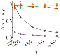
() Vary $n$

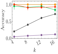
(a) Vary $k$

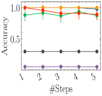
(b) Vary #steps

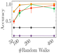
(c) Vary #walks

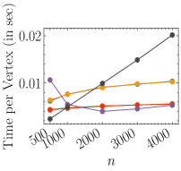
(d) Vary $n$: avg. query time

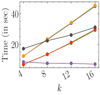
(e) Vary $k$: time

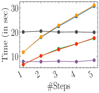
(f) Vary #steps: time

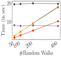
(g) Vary #walks: time

Figure 3: Clustering results on synthetic data. We consider varying number of vertices $n$ (Figs. 3() and 3(d)), varying number of communities $k$ (Figs. 3(a) and 3(e)), varying random walk length (Figs. 3(b) and 3(f)), and varying number of random walks (Figs. 3(c) and 3(g)). Figs. 3()–3(c) report the clustering accuracies, Fig. 3(d) reports the running time per vertex in seconds, and Figs. 3(e)–3(g) report total running times in seconds. Markers are mean values and error bars are one standard deviation over 5 datasets.

In Fig. 3() we vary the number of vertices $n$ while keeping $k=6$ fixed. rw-seeded and rw-u-seeded deliver almost perfect accuracy, i.e., they classify almost all vertices correctly; we note that in the plot, the lines of rw-seeded and rw-u-seeded are essentially identical and thus the line for rw-seeded is hard to see. rw-unseeded and rw-u-unseeded also deliver good results. Furthermore, polarSeeds works well when the clusters are small (for $n=500$ there are 83 vertices in each cluster) but its performance decays as the clusters get larger. FOCG generally returns clusterings of low quality because it returns many clusters of very small sizes.

In Fig. 3(a), we fix $n$ and vary $k=4,8,12,16$. Again, we observe a similar behavior as before: our oracles outperform the competitors, and the competitors improve for smaller clusters ($k$ larger).

We also varied the parameters for the oracles. In Fig. 3(b), we set the number of random walk steps to $1,2,3,4,5$. We see that even with very short random walks, the algorithms deliver very good results. However, as the number of steps increases, the solution quality slightly decreases (see, e.g., rw-seeded or rw-u-unseeded). This confirms the theoretical analysis of Lem.s 9 and 10.

In Fig. 3(c), we set the random walks lengths to $50,100,200,4000$. rw-seeded and rw-u-seeded return excellent clusterings when at least $200\approx 4.5\cdot\sqrt{n}$ random walks are performed.

In Figs. 3(d)–3(g) we report the running times of the algorithms. Our oracles scale linearly in the number of steps (Fig. 3(f)), and the number of random walks (Fig. 3(g)). Furthermore, since our number of seed nodes depends on the number of communities $k$, the oracles scale linearly in $k$ (Fig. 3(e)). In Fig. 3(d) we report the running time, normalized by the number of vertices in the graph; for our oracle data structures this corresponds to the time they spend on each query. We observe that the query times of the oracles increases only very moderately as the number of vertices $n$ increases; we blame this slight increase on the internal data structures (such as hash maps) that we use to store our graphs. This is in contrast to polarSeeds, for which the running time per vertex is increasing (Fig. 3(d)). For FOCG we observe that it scales linearly in the number of vertices (since in Fig. 3(d) the average time per vertex is nearly constant for $n\geq 1000$) and its running time slightly decreases as it finds better communities (Figs. 3(a) and 3(e))

Biclustering experiments. In Fig. 4 we present our results for finding biclusters $(V_{1},V_{2}),(V_{3},V_{4}),\dots,(V_{2k-1},V_{2k})$. Thus, we run the biclustering versions of the algorithms. The oracles used $t=2$ random walk steps and $R=600$ random walks, unless stated otherwise. The seeded oracles and polarSeeds obtained 3 seed vertices from each $V_{i}$; the unseeded oracles randomly sampled $6k$ seed vertices in the preprocessing.

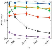
() Vary $n$

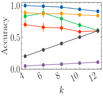
(a) Vary $k$

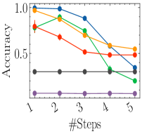
(b) Vary #steps

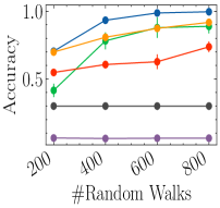
(c) Vary #walks

Figure 4: Biclustering results on synthetic data. We vary the number of vertices $n$ (Fig. 4()), the number of communities $k$ (Fig. 4(a)), the random walk length (Fig. 4(b)) and the number of random walks (Fig. 4(c)). We report the achieved accuracies; markers are mean values over 5 different datasets, and error bars are one standard deviation over the 5 datasets.

Again, our oracles obtain better results than the baseline algorithms, which typically return too small clusters. Furthermore, the signed oracles rw-seeded and rw-unseeded outperform the unsigned oracles rw-u-seeded and rw-u-unseeded, resp. This shows that the edge signs are necessary to split the clusters $U_{i}$ into biclusters $V_{2i-1}$ and $V_{2i}$. Compared to the clustering setting from before, the biclustering algorithms are more sensitive to the number steps (Fig. 4(b)), and they also require more random walks (Fig. 4(c)).

Conclusion. Our experiments suggest that our oracles outperform the baselines when the clusters are large. Also, to recover the biclusters $(V_{2i-1},V_{2i})$, it is necessary to use the edge signs. Furthermore, the seeded methods outperform the unseeded methods.

References

- Atay & Liu (2020) Atay, F. M. and Liu, S. Cheeger constants, structural balance, and spectral clustering analysis for signed graphs. Discrete Mathematics, 343(1):111616, 2020.
- Bansal et al. (2004) Bansal, N., Blum, A., and Chawla, S. Correlation clustering. Mach. Learn., 56(1-3):89–113, 2004.
- Bonchi et al. (2019) Bonchi, F., Galimberti, E., Gionis, A., Ordozgoiti, B., and Ruffo, G. Discovering polarized communities in signed networks. In Proceedings of the 28th ACM International Conference on Information and Knowledge Management, pp. 961–970, 2019.
- Cesa-Bianchi et al. (2012) Cesa-Bianchi, N., Gentile, C., Vitale, F., and Zappella, G. A correlation clustering approach to link classification in signed networks. In Mannor, S., Srebro, N., and Williamson, R. C. (eds.), COLT, volume 23, pp. 34.1–34.20, 2012.
- Chiang et al. (2012) Chiang, K., Whang, J. J., and Dhillon, I. S. Scalable clustering of signed networks using balance normalized cut. In CIKM, pp. 615–624. ACM, 2012.
- Chiang et al. (2014) Chiang, K., Hsieh, C., Natarajan, N., Dhillon, I. S., and Tewari, A. Prediction and clustering in signed networks: a local to global perspective. J. Mach. Learn. Res., 15(1):1177–1213, 2014.
- Chiplunkar et al. (2018) Chiplunkar, A., Kapralov, M., Khanna, S., Mousavifar, A., and Peres, Y. Testing graph clusterability: Algorithms and lower bounds. CoRR, abs/1808.04807, 2018. URL http://arxiv.org/abs/1808.04807. Conference version appeared in FOCS 2018.
- Chu et al. (2016) Chu, L., Wang, Z., Pei, J., Wang, J., Zhao, Z., and Chen, E. Finding gangs in war from signed networks. In KDD, pp. 1505–1514, 2016.
- Chung (1997) Chung, F. R. Spectral Graph Theory. Number 92. American Mathematical Soc., 1997.
- Csardi & Nepusz (2006) Csardi, G. and Nepusz, T. The igraph software package for complex network research. InterJournal, Complex Systems:1695, 2006. URL https://igraph.org.
- Cucuringu et al. (2019) Cucuringu, M., Davies, P., Glielmo, A., and Tyagi, H. SPONGE: A generalized eigenproblem for clustering signed networks. In AISTATS, volume 89, pp. 1088–1098. PMLR, 2019.
- Cucuringu et al. (2020) Cucuringu, M., Singh, A. V., Sulem, D., and Tyagi, H. Regularized spectral methods for clustering signed networks. CoRR, abs/2011.01737, 2020.
- Czumaj et al. (2015) Czumaj, A., Peng, P., and Sohler, C. Testing cluster structure of graphs. CoRR, abs/1504.03294, 2015. URL http://arxiv.org/abs/1504.03294. Conference version appeared in STOC 2015.
- Gharan & Trevisan (2014) Gharan, S. O. and Trevisan, L. Partitioning into expanders. In Proceedings of the twenty-fifth annual ACM-SIAM symposium on Discrete algorithms, pp. 1256–1266. SIAM, 2014.
- Gluch et al. (2021) Gluch, G., Kapralov, M., Lattanzi, S., Mousavifar, A., and Sohler, C. Spectral clustering oracles in sublinear time. CoRR, abs/2101.05549, 2021. Conference version appeared in SODA 2021.
- Harary (1953) Harary, F. On the notion of balance of a signed graph. Michigan Mathematical Journal, 2(2):143–146, 1953.
- Jung et al. (2016) Jung, J., Jin, W., Sael, L., and Kang, U. Personalized ranking in signed networks using signed random walk with restart. In ICDM, pp. 973–978, 2016.
- Jung et al. (2020) Jung, J., Jin, W., and Kang, U. Random walk-based ranking in signed social networks: model and algorithms. Knowl. Inf. Syst., 62(2):571–610, 2020.
- Kunegis et al. (2010) Kunegis, J., Schmidt, S., Lommatzsch, A., Lerner, J., De Luca, E. W., and Albayrak, S. Spectral analysis of signed graphs for clustering, prediction and visualization. In SDM, pp. 559–570, 2010.
- Mercado et al. (2016) Mercado, P., Tudisco, F., and Hein, M. Clustering signed networks with the geometric mean of laplacians. In NIPS, pp. 4421–4429, 2016.
- Mercado et al. (2019) Mercado, P., Tudisco, F., and Hein, M. Spectral clustering of signed graphs via matrix power means. In ICML, pp. 4526–4536, 2019.
- Ordozgoiti et al. (2020) Ordozgoiti, B., Matakos, A., and Gionis, A. Finding large balanced subgraphs in signed networks. In WWW, pp. 1378–1388, 2020.
- Peng (2020) Peng, P. Robust Clustering Oracle and Local Reconstructor of Cluster Structure of Graphs. In SODA, pp. 2953–2972, 2020.
- Pons & Latapy (2006) Pons, P. and Latapy, M. Computing communities in large networks using random walks. J. Graph Algorithms Appl., 10(2):191–218, 2006.
- Trevisan (2012) Trevisan, L. Max cut and the smallest eigenvalue. SIAM Journal on Computing, 41(6):1769–1786, 2012.
- Xiao et al. (2020) Xiao, H., Ordozgoiti, B., and Gionis, A. Searching for polarization in signed graphs: a local spectral approach. In WWW, pp. 362–372, 2020.