Joint Precoding for Active Intelligent Transmitting Surface Empowered Outdoor-to-Indoor Communication in mmWave Cellular Networks

Abstract

Outdoor-to-indoor communications in millimeter-wave (mmWave) cellular networks have been one challenging research problem due to the severe attenuation and the high penetration loss caused by the propagation characteristics of mmWave signals. We propose a viable solution to implement the outdoor-to-indoor mmWave communication system with the aid of an active intelligent transmitting surface (active-ITS), where the active-ITS allows the incoming signal from an outdoor base station (BS) to pass through the surface and be received by the indoor user-equipments (UEs) after shifting its phase and magnifying its amplitude. Then, the problem of joint precoding of the BS and active-ITS is investigated to maximize the weighted sum-rate (WSR) of the communication system. An efficient block coordinate descent (BCD) based algorithm is developed to solve it with the suboptimal solutions in nearly closed-forms. In addition, to reduce the size and hardware cost of an active-ITS, we provide a block-amplifying architecture to partially remove the circuit components for power-amplifying, where multiple transmissive-type elements (TEs) in each block share a same power amplifier. Simulations indicate that active-ITS has the potential of achieving a given performance with much fewer TEs compared to the passive-ITS under the same total system power consumption, which makes it suitable for application to the size-limited and aesthetic-needed scenario, and the inevitable performance degradation caused by the block-amplifying architecture is acceptable.

I Introduction

Millimeter-wave (mmWave) cellular networks are capable of supplying the ever-increasing demand of rates for advanced fifth-generation communications thanks to their abundant available bandwidth. However, a fundamental challenge for mmWave communications is that the mmWave signal experience a severe attenuation and a high penetration loss compared with the lower frequency bands, which makes mmWave signals highly vulnerable to obstacles [1, 2, 3]. The emerging technique of reconfigurable intelligent surfaces (RISs) have been proposed as a promising candidate for alleviating the unfavorable properties of mmWave signals. RIS is an ultra-thin metasurface comprising multiple programmable elements, which enables to achieve a high beamforming gain by smartly manipulating the incident signal for proactively customizing the radio propagation environment [4, 5, 6]. More importantly, RIS can significantly reduce the outage caused by the presence of random blockages through establishing virtual line-of-sight (LoS) links between base stations (BSs) and user equipments (UEs), which can considerably enhance the reliability of mmWave communications, especially in harsh urban propagation environments [7, 8, 9]. These benefits have inspired a lot of work to investigate RIS-assisted mmWave communication networks and verify that RIS in favor of enhancing the signal strength, extending the service range, and improving the spectral- and energy-efficiency [10, 11, 12, 13].

On the other hand, outdoor-to-indoor communication in mmWave cellular networks is a common communication scenario as the most mobile data traffic is consumed indoors, however, which is challenging since BSs and UEs are located on the opposite side of building structures [14], e.g., walls and windows, while penetrating them leads a severe attenuation (measurements have shown that around 40 and 28 dB for tinted-glass and brick [15], respectively), which limits the feasibility for an outdoor BS communicates with indoor UEs inside the buildings. Relay enabled system is a potential solution for outdoor-to-indoor mmWave communications but has some drawbacks, e.g., expensive hardware components and high signal processing complexity [16], while these shortcomings of relays can be overcome by utilizing the superiority of the RISs [17, 18]. However, the widely studied RISs-assisted systems focused on traditional reflective-type RISs, also referred to intelligent reflecting surfaces (IRSs) [19], as objects hanging on walls or facades of buildings, which face a placement restriction: both BSs and UEs have to be located on the front side of an IRS, and hence IRSs can only achieve a half-space coverage and are not up to the outdoor-to-indoor communication. As a remedy, some works [20, 21] innovative deployed multiple IRSs in a cooperative multi-hop manner to bypass the obstacle. Nevertheless, this does not apply to outdoor-to-indoor communications due to no matter where IRSs are placed, the signal after reflecting cannot bypass the wall to UEs behind the IRSs [17, 19].

To challenge this restriction and facilitate more flexible deployment of RIS, the novel concept of transmissive(refractive)-type RIS, also named intelligent transmitting surfaces (ITS) has been proposed [22, 23]. ITS is a meta-material reflection-less surface structure [24], which is equipped with a large number of transmissive-type elements (TEs), provides beam shaping, steering, and focus capabilities [25]. A key feature of ITS is that the incoming signal can pass through each TE, and then the refracted signal can be received by UEs behind the ITS. More importantly, ITSs can be flexibly deployed by coexisting with existing infrastructures in the middle of a communication environment, such as embedded in walls or windows between two different environments (outdoor-to-indoor, room-to-room, etc.) [19, 17]. ITSs can fully unleash the potential of RISs on breaking the half-space (reflection space) limitation of signal propagation manipulated by IRS, and so that covers the back side space (transmission space) .

However, identically with the reflective cascaded channel in the IRS-assisted communication, the transmissive cascaded channel in the ITS-assisted communication will still suffer a multiplicative fading effect [30], which potentially causes the ITS achieve a poor performance gain. A common approach to improve the performance gain of RISs is increasing the number of reflective-type elements (REs) or TEs [31]. Intuitively speaking, this approach is feasible for the IRS but might not be practical for the ITS due to that the number of TEs is limited by the physical size of windows and the aesthetic appearance effect, which might be the price to be paid for that the ITS is embedded with existing building structures [19]. Additionally, the substantial electromagnetic penetration loss when the mmWave signal impinges upon and penetrates the ITS cannot be negligible [17]. These concerns imply that the performance gain reaped by the ITS might be worthy weak.

To this end, the deployment of an active-ITS will bring a notable leap forward for improving performance in the outdoor-to-indoor mmWave communication. The noticeable difference between the active-ITS and the passive-ITS is that the former can refract the incoming signals after amplifying amplitudes and shifting phases simultaneously, rather than only refracting them after changing phases as done by the latter, which offer an extra flexibility to reconfigure the incident signal. Identical to the principle of active REs [32, 33, 34], an active TE equips with an additional power amplifier for magnifying the signal amplitude [35]. In this way, active-ITS brings an extra degree of freedom (DOF) in the beamforming, and the number of TEs of active-ITS can be beneficially reduced compared with the passive-ITS with a same performance [36, 37]. The active-ITS seems to act as an active concave lens [13] that directly refracts the incident signal with power amplification at the electromagnetic level. Nevertheless, it still takes the advantages of the passive-ITS that does not have expensive and power-consuming ratio-frequency (RF) chains, and hence has no capability for signal processing [38, 39, 40], which is fundamentally different from conventional amplify-and-forward (AF) relays [30].

Motivated by the above background, we aim to utilize the superiority of an active-ITS to alleviate the negative effects of the mmWave signal so that to implement the challenging but important outdoor-to-indoor communication system in the mmWave cellular network with a high performance. Particularly, the main contributions of this paper are summarized as follows:

• To our best knowledge, this is the first work to implement outdoor-to-indoor mmWave communication with the aid of an active-ITS, where the incoming signal can be refracted to the back side of the active-ITS after magnifying its amplitude and manipulating its phase.

• To jointly optimize the precoding matrix of both the BS and active-ITS in the outdoor-to-indoor mmWave communication system, we formulate a weighted sum-rate (WSR) maximization problem, which is non-convex and challenging to obtain its corresponding globally optimal solution. Consequently, we propose a compromising approach to solve it, where the original problem is transformed into an equivalent form, and then a block coordinate descent (BCD) based algorithm is employed to obtain the suboptimal solutions in nearly closed-forms of the linear precoding matrix of the BS, and the power amplification factor matrix and the transmissive phase-shifting matrix of the active-ITS.

• In order to reduce the size and hardware cost of the active-ITS, we provide a block-amplifying architecture to partially remove the circuit components for power-amplifying, where multiple TEs in each block share a same power amplifier. Then, we extend the proposed algorithm under the element-amplifying architecture to jointly optimize the precoding matrix under the block-amplifying architecture.

• Simulation results demonstrate that the active-ITS can significantly improve the WSR performance of the outdoor-to-indoor mmWave communication system, and the inevitable performance loss caused by the block-amplifying ITS architecture is acceptable.

The organization of the rest of this work is organized as follows. In Section II, we describe the active-ITS empowered outdoor-to-indoor communications in the mmWave cellular network model, and formulate the WSR maximization problem. In Section III, we propose an efficient joint design algorithm to solve it. Then, in Section IV, the proposed algorithm is extended to solve the problem with the block-amplifying ITS architecture. Simulation results are presented in Section V, and finally the paper is concluded in Section VI.

Notations: Scalars, vectors, and matrices are presented by lower-case, bold-face lower-case, and bold-face upper-case letters, respectively. $\mathcal{C}\mathcal{N}\left(\mathbf{0},\mathbf{I}\right)$ denotes the circularly symmetric complex Gaussian (CSCG) distribution with zero mean and covariance matrix $\mathbf{I}_{N}$, where $\mathbf{I}_{N}$ denotes an $N\times N$ identity matrix. $\operatorname{Vecd}\left\{\cdot\right\}$ forms a vector out of the diagonal of its matrix argument. $\circ$ denote the Hadamard products. $\mathbf{A}^{\operatorname{H}}$ and $\operatorname{Tr}\left(\mathbf{A}\right)$ denote the Hermitian and trace operators of matrix $\mathbf{A}$, respectively. $\operatorname{Re}\left\{a\right\}$ is the real part of a scalar $a$.

II SYSTEM MODEL AND PROBLEM FORMULATION

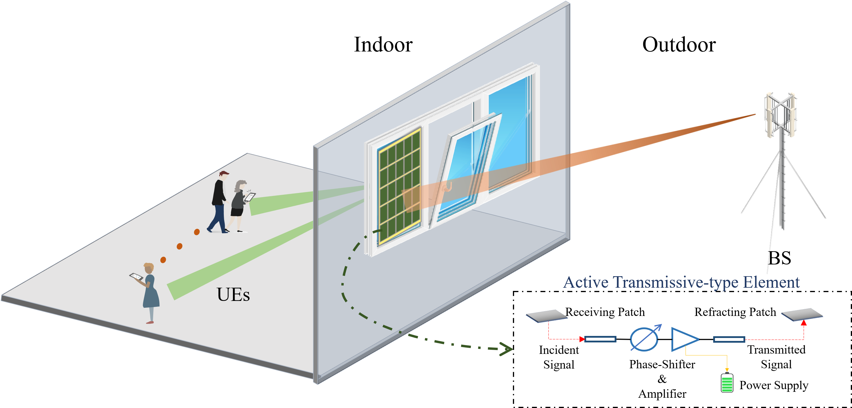
Fig. 1: A system model schematic of the active-ITS empowered outdoor-to-indoor mmWave communication.

As shown in Fig. 1, we consider the downlink of an outdoor-to-indoor mmWave communication scenario, where the direct-link channels from the BS to UEs are assumed severely blocked by the concrete-wall and the tinted-glass, and hence, fall into almost complete outage [10]. Thanks to the transmissive characteristic of the ITS, the incoming mmWave signal can pass through the surface when impinge upon it, and hence, the signal can be refracted from the outdoor BS to the indoor UEs through the ITS. To alleviate the severe attenuation of mmWave signals and greatly reduce the number of TEs of the ITS for application to the size-limited window, we assume each active TE of the ITS can not only shift the phase of the incident signal, but also amplify the amplitude of the incident signal with the aid of the power supply [35]. In addition, a smart controller is attached to the active-ITS and responsible to operate the active-ITS with the transmissive coefficients, which are coordinated by the BS [22, 41, 42, 43].

II-A Channel Model

Let $M_{t}$, $M_{r}$, and $N$ denote the number of the transmitting antennas, the receiving antennas, and the TEs equipped by the BS, UEs, and active-ITS, respectively. The complicated uniform planar arrays (UPA) antenna configuration is employed at the BS, UEs, and active-ITS, which is more practical than uniform linear array (ULA) for RIS-assisted systems[11]. In addition, due to the low diffraction from objects of mmWave signals, mmWave channels are usually characterized according to the widely used Saleh-Valenzuela model [10, 11, 12, 13]. Hence, the channel matrices from the BS to the active-ITS and from the active-ITS to the $k$-th UE are denoted by $\mathbf{G}\in\mathbb{C}^{N\times M_{t}}$ and $\mathbf{H}_{k}\in\mathbb{C}^{N\times M_{r}},\forall k\in K$, respectively, which can be mathematically determined as follows

$$\mathbf{G} =\sqrt{\frac{M_{t}N}{L_{\text{BI}}}}\sum\nolimits_{l=1}^{L_{\text{BI}}}{\alpha_{l}\mathbf{a}_{\text{ITS}}\left(\nu_{l}^{\text{AOA}},\vartheta_{l}^{\text{AOA}}\right)\mathbf{a}_{\text{BS}}^{\operatorname{H}}\left(\nu_{l}^{\text{AOD}},\vartheta_{l}^{\text{AOD}}\right)},$$ (1a)

$$\mathbf{H}_{k} =\sqrt{\frac{M_{r}N}{P_{\text{IU}}}}\sum\nolimits_{p=1}^{P_{\text{IU}}}{\beta_{p}\mathbf{a}_{\text{UE}}\left(\nu_{p}^{\text{AOA}},\vartheta_{p}^{\text{AOA}}\right)\mathbf{a}_{\text{ITS}}^{\operatorname{H}}\left(\nu_{p}^{\text{AOD}},\vartheta_{p}^{\text{AOD}}\right)},\forall k\in K,$$ (1b)

where $L_{\text{BI}}$ and $P_{\text{IU}}$ are the number of propagation paths between the BS and the active-ITS, and between the active-ITS and the $k$-th UE, and where variables $\alpha_{l}$ and $\beta_{p}$ denote the complex gains for links, with $l=1$ and $p=1$ stand for the LoS path and the remaining are NLoS paths. $\mathbf{a}_{\text{BS}}\left(\nu_{l}^{\text{AOD}},\vartheta_{l}^{\text{AOD}}\right)$ and $\mathbf{a}_{\text{ITS}}\left(\nu_{p}^{\text{AOD}},\vartheta_{p}^{\text{AOD}}\right)$ are transmit array response vectors of the BS and the active-ITS, $\mathbf{a}_{\text{UE}}\left(\nu_{l}^{\text{AOA}},\vartheta_{l}^{\text{AOA}}\right)$ and $\mathbf{a}_{\text{ITS}}\left(\nu_{p}^{\text{AOA}},\vartheta_{p}^{\text{AOA}}\right)$ are receive array response vectors of the UEs and the active-ITS, respectively, where $\nu^{\text{AOA}}$ ($\nu^{\text{AOD}}$) and $\vartheta^{\text{AOA}}$ ($\vartheta^{\text{AOD}}$) denote the azimuth and elevation angles of arrival (departure), respectively. The typical array response vector for the UPA model can be mathematically expressed by

$$\mathbf{a}\left(\nu,\vartheta\right)= \frac{1}{\sqrt{HV}}\left[1,\cdots,e^{j\frac{2\pi d}{\lambda}\left(h\sin\left(\vartheta\right)\sin\left(\nu\right)+v\cos\left(\vartheta\right)\right)},\right.$$

$$\qquad\qquad\qquad\qquad\cdots,\left.e^{j\frac{2\pi d}{\lambda}\left(\left(H-1\right)\sin\left(\vartheta\right)\sin\left(\nu\right)+\left(V-1\right)\cos\left(\vartheta\right)\right)}\right]^{\operatorname{T}},$$ (2)

where $H$ and $V$ denote the number of TEs (antennas) in the horizontal and vertical directions of the active-ITS (BS/UEs), and the element spacing is set to be $d=\lambda/2$. To unveil the theoretical upper bound of performance gain achieved by the active-ITS, we follow the assumption [29, 18, 41, 42, 43] that the full instantaneous channel state information (CSI) knowledge can be perfectly estimated at the BS and all the calculations are performed at the BS.

II-B System Model

Let $\mathbf{A}=\operatorname{diag}\left(a_{1},a_{2},\cdots,a_{N}\right)\in\mathbb{R}^{N\times N}$ and $\bm{\Theta}=\operatorname{diag}\left(e^{j\varphi_{1}},e^{j\varphi_{2}},\cdots,e^{j\varphi_{N}}\right)\in\mathbb{C}^{N\times N}$ represent the power amplification factor matrix and the transmissive phase-shifting matrix at the active-ITS with $a_{n}\geq 1$ and $\varphi_{n}\in\left[0,2\pi\right)$, $\forall n\in N$.

The signal from the BS is given by $\mathbf{x}=\sum_{k=1}^{K}{\mathbf{W}_{k}\mathbf{s}_{k}},\forall k\in K$, where $\mathbf{s}_{k}\in\mathbb{C}^{s\times 1}$ represents $s$ desired streams for the $k$-th UE and satisfies $\mathbf{s}_{k}\sim\mathcal{C}\mathcal{N}\left(\bm{0}_{s},\mathbf{I}_{s}\right)$, and $\mathbf{W}_{k}\in\mathbb{C}^{M_{t}\times s}$ denotes the linear precoding matrix. As a result, the signal received at the active-ITS is given by

$$\mathbf{y}_{\operatorname{ITS}}^{r}=\mathbf{G}\mathbf{x}+\bm{\upsilon},$$ (3)

where $\bm{\upsilon}\in\mathbb{C}^{N\times 1}$ is additive white Gaussian noise (AWGN) and satisfying $\bm{\upsilon}\sim\mathcal{C}\mathcal{N}\left(\bm{0}_{N},\delta^{2}\mathbf{I}_{N}\right)$.

Then, by employing an active-ITS, the refracted signal can be denoted by

$$\mathbf{y}_{\operatorname{ITS}}^{t}=\kappa\mathbf{A}\bm{\Theta}\left(\mathbf{G}\mathbf{x}+\bm{\upsilon}\right),$$ (4)

where $\kappa$ characterizes the extent of loss corresponding to the absorption and the reflection of the signal power when the mmWave signal impinges upon and penetrates the ITS. The noise $\bm{\upsilon}$ after power amplifying cannot be negligible, which is significantly different from the conventional passive-ITS [33]. For simplicity of presentation, let $\bm{\Phi}\triangleq\mathbf{A}\circ\bm{\Theta}$ denotes the transmissive coefficient matrix, where each diagonal element is denoted by $\Phi_{n,n}=a_{n}e^{j\varphi_{n}},\forall n\in N$.

The signal received by the $k$-th UE can be mathematically expressed as follows

$$\mathbf{y}_{k}= \kappa\mathbf{H}_{k}^{\operatorname{H}}\mathbf{\Phi}\mathbf{G}\mathbf{W}_{k}\mathbf{s}_{k}+\sum\nolimits_{i=1,i\neq k}^{K}{\kappa\mathbf{H}_{k}^{\operatorname{H}}\mathbf{\Phi}\mathbf{G}\mathbf{W}_{i}\mathbf{s}_{i}}+\kappa\mathbf{H}_{k}^{\operatorname{H}}\mathbf{\Phi}\bm{\upsilon}+\mathbf{n}_{k},\forall k\in K,$$ (5)

where $\mathbf{n}_{k}\in\mathbb{C}^{M_{r}\times 1}$ represents the thermal noise at the $k$-th UE and satisfying $\mathbf{n}_{k}\sim\mathcal{C}\left(\bm{0}_{M_{r}},\sigma_{k}^{2}\mathbf{I}_{M_{r}}\right)$.

Therefore, the signal-to-interference-plus-noise-ratio (SINR) at the $k$-th UE is given by

$$\bm{\Gamma}_{k}=\kappa^{2}\mathbf{H}_{k}^{\operatorname{H}}\mathbf{\Phi}\mathbf{G}\mathbf{W}_{k}\mathbf{W}_{k}^{\operatorname{H}}\mathbf{G}^{\operatorname{H}}\mathbf{\Phi}^{\operatorname{H}}\mathbf{H}_{k}\mathbf{V}_{k}^{\operatorname{-1}},\forall k\in K,$$ (6)

where $\mathbf{V}_{k}$ denotes the interference-plus-noise covariance matrix and can be expressed by

$$\mathbf{V}_{k} =\sum\nolimits_{i=1,i\neq k}^{K}{\kappa^{2}\mathbf{H}_{k}^{\operatorname{H}}\mathbf{\Phi}\mathbf{G}\mathbf{W}_{i}\mathbf{W}_{i}^{\operatorname{H}}\mathbf{G}^{\operatorname{H}}\mathbf{\Phi}^{\operatorname{H}}\mathbf{H}_{k}}+\kappa^{2}\delta^{2}\mathbf{H}_{k}^{\operatorname{H}}\mathbf{\Phi}\mathbf{\Phi}^{\operatorname{H}}\mathbf{H}_{k}+\sigma_{k}^{2}\mathbf{I}_{M_{r}},\forall k\in K.$$ (7)

Accordingly, the achievable data rate of the $k$-th UE is given by

$$\mathcal{R}_{k}=\log\left|\mathbf{I}+\bm{\Gamma_{k}}\right|,\forall k\in K.$$ (8)

II-C Problem Formulation

In this paper, we aim to maximize the WSR of the outdoor-to-indoor mmWave communication system by joint optimizing the linear precoding matrix at the BS, i.e., $\mathbf{W}$, and the transmissive coefficient matrix at the active-ITS, i.e., $\bm{\Phi}$, while satisfying the constraints of the maximum power budgets at the BS and active-ITS, and the transmissive phase-shifting at each TE. Based on the above discussions, the WSR maximization problem can be formulated as follows

$$\mathcal{P}_{1}:\mathop{\max}_{\mathbf{W},\mathbf{\Phi}}\quad \mathcal{R}\left(\mathbf{W},\mathbf{\Phi}\right)={\sum\nolimits_{k=1}^{K}{\alpha_{k}\log\left|\mathbf{I}+\bm{\Gamma_{k}}\right|}},$$ (9a)

$$\operatorname{s.t.}\quad \sum\nolimits_{k=1}^{K}{\|\mathbf{W}_{k}\|_{\operatorname{F}}^{2}}\leq P_{\operatorname{BS}}^{\max},$$ (9b)

$$\sum\nolimits_{k=1}^{K}{\kappa^{2}\|\mathbf{\Phi}\mathbf{G}\mathbf{W}_{k}\|_{\operatorname{F}}^{2}}+\delta^{2}\kappa^{2}\|\mathbf{\Phi}\|_{\operatorname{F}}^{2}\leq P_{\operatorname{ITS}}^{\max},$$ (9c)

$$\angle\bm{\Phi}_{n,n}\in\left[0,2\pi\right),\forall n\in N,$$ (9d)

where $\bm{\alpha}=\left[\alpha_{1},\alpha_{2},\cdots,\alpha_{K}\right]$ denotes the weighting factor vector with each element $\alpha_{k}$ is a predetermined value depending on the fairness and the required quality of service for applications, and where $P_{\operatorname{BS}}^{\max}$ and $P_{\operatorname{ITS}}^{\max}$ are the budgets of the transmission power and the amplification power at the BS and the active-ITS, respectively.

Remark 1: If we remove the amplifying power budget constraint in (9c) and set $\mathbf{A}=\mathbf{I}$, Problem $\mathcal{P}_{1}$ reduce to the WSR maximization problem for conventional passive-RIS assisted communication systems [41, 42, 43]. However, the additional constraint and the optimization of the power amplification factor matrix [44] make Problem $\mathcal{P}_{1}$ even more challenging to solve.

III The Proposed Suboptimal Joint Precoding Algorithm

The formulated problem $\mathcal{P}_{1}$ is non-convex and arduous to tackle optimally, in this section, we propose an efficient joint precoding algorithm to handle it with suboptimal solutions. Particularly, to facilitate the solution development, we first reformulate the original problem as an equivalent but tractable form, and then a BCD-based method is provided to solve the transformed problem.

III-A Problem Reformulation and Decomposition

First, to deal with the complexity of the objective function in the formulated WSR maximization problem $\mathcal{P}_{1}$, we transform it into an equivalent weighted minimum mean-square error (WMMSE) minimization problem [45, 41, 42].

Let us assume that the MMSE estimator $\mathbf{U}=\left\{\mathbf{U}_{k}\in\mathbb{C}^{M_{r}\times s},\forall k\in K\right\}$ are applied to UEs, and accordingly, the estimated signal vector of the $k$-th UE is given by

$$\mathbf{\hat{s}}_{k}=\mathbf{U}_{k}^{\operatorname{H}}\mathbf{y}_{k},\forall k\in K.$$ (10)

Therefore, the MMSE matrix of the $k$-th UE is given by

$$\mathbf{E}_{k}= \mathbb{E}_{\mathbf{x},\bm{\upsilon},\mathbf{n}}\left[\left(\mathbf{\hat{s}}_{k}-\mathbf{s}_{k}\right)\left(\mathbf{\hat{s}}_{k}-\mathbf{s}_{k}\right)^{\operatorname{H}}\right]$$

$$= \sum\nolimits_{i=1}^{K}{\kappa^{2}\mathbf{U}_{k}^{\operatorname{H}}\mathbf{H}_{k}^{\operatorname{H}}\mathbf{\Phi}\mathbf{G}\mathbf{W}_{i}\mathbf{W}_{i}^{\operatorname{H}}\mathbf{G}^{\operatorname{H}}\mathbf{\Phi}^{\operatorname{H}}\mathbf{H}_{k}\mathbf{U}_{k}}+\kappa^{2}\delta^{2}\mathbf{U}_{k}^{\operatorname{H}}\mathbf{H}_{k}^{\operatorname{H}}\mathbf{\Phi}\mathbf{\Phi}^{\operatorname{H}}\mathbf{H}_{k}\mathbf{U}_{k}$$

$$+\sigma_{k}^{2}\mathbf{U}_{k}^{\operatorname{H}}\mathbf{U}_{k}+\mathbf{I}_{s}-\kappa\mathbf{U}_{k}^{\operatorname{H}}\mathbf{H}_{k}^{\operatorname{H}}\mathbf{\Phi}\mathbf{G}\mathbf{W}_{k}-\kappa\mathbf{W}_{k}^{\operatorname{H}}\mathbf{G}^{\operatorname{H}}\mathbf{\Phi}^{\operatorname{H}}\mathbf{H}_{k}\mathbf{U}_{k},\forall k\in K.$$ (11)

By introducing an auxiliary variable $\mathbf{F}_{k}\in\mathbb{C}^{s\times s}$ for the $k$-th UE and defining $\mathbf{F}=\left\{\mathbf{F}_{k},\forall k\in K\right\}$, problem $\mathcal{P}_{1}$ can be equivalently transformed into

$$\mathcal{P}_{2}:\mathop{\max}_{\mathbf{F},\mathbf{U},\mathbf{W},\mathbf{\Phi}}\; {\sum\nolimits_{k=1}^{K}{\alpha_{k}h_{k}\left(\mathbf{F},\mathbf{U},\mathbf{W},\mathbf{\Phi}\right)}}$$ (12a)

$$\operatorname{s.t.}\; \eqref{p11}-\eqref{p13},$$ (12b)

where $h_{k}\left(\mathbf{F},\mathbf{U},\mathbf{W},\mathbf{\Phi}\right)=\log\left|\mathbf{F}_{k}\right|-\operatorname{Tr}\left(\mathbf{F}_{k}\mathbf{E}_{k}\right)+s,\forall k\in K$.

Although the above problem has been significantly simplified compared with problem $\mathcal{P}_{1}$, it is still challenging to tackle. Fortunately, based on the fact that the objective function in (12a) is concave with respect to any one of the four variables (i.e., $\mathbf{U}$, $\mathbf{F}$, $\mathbf{W}$, and $\bm{\Phi}$) when the other three variables being fixed, which makes the problem more amenable. In the following, we provide an efficient BCD-based algorithm for solving problem $\mathcal{P}_{2}$ in an iterative manner.

Note that the MMSE decoding matrix $\mathbf{U}$ and the auxiliary matrix $\mathbf{F}$ do not exist in any constraints in problem $\mathcal{P}_{2}$, which implies that with fixed $\mathbf{W}$ and $\bm{\Theta}$, the calculation of $\mathbf{F}^{\star}$ and $\mathbf{U}^{\star}$ constitute a pair of unconstrained optimization problems. Therefore, the optimal solutions can be obtained by setting the first-order partial derivatives of the objective function of problem $\mathcal{P}_{2}$ with respect to $\mathbf{U}_{k},\forall k\in K$ and $\mathbf{F}_{k},\forall k\in K$ to be zeros, respectively. After some matrix manipulations, the optimal closed-form solutions can be respectively determined by

$$\mathbf{U}_{k}^{\star}=\left(\mathbf{\bar{V}}_{k}\right)^{\operatorname{-1}}\mathbf{H}_{k}^{\operatorname{H}}\mathbf{\Phi}\mathbf{G}\mathbf{W}_{k},\forall k\in K,$$ (13)

where $\mathbf{\bar{V}}_{k}=\mathbf{V}_{k}+{\kappa^{2}\mathbf{H}_{k}^{\operatorname{H}}\mathbf{\Phi}\mathbf{G}\mathbf{W}_{k}\mathbf{W}_{k}^{\operatorname{H}}\mathbf{G}^{\operatorname{H}}\mathbf{\Phi}^{\operatorname{H}}\mathbf{H}_{k}}$, and

$$\mathbf{F}_{k}^{\star}=\left(\mathbf{E}_{k}^{\star}\right)^{\operatorname{-1}},\forall k\in K,$$ (14)

where $\mathbf{E}_{k}^{\star}$ is determined by

$$\mathbf{E}_{k}^{\star}=\mathbf{I}_{s}-\mathbf{W}_{k}^{\operatorname{H}}\mathbf{G}^{\operatorname{H}}\bm{\Phi}^{\operatorname{H}}\mathbf{H}_{k}\mathbf{\bar{V}}_{k}^{\operatorname{-1}}\mathbf{H}_{k}^{\operatorname{H}}\bm{\Phi}\mathbf{G}\mathbf{W}_{k},\forall k\in K.$$ (15)

Once both $\mathbf{U}^{\star}$ and $\mathbf{F}^{\star}$ are determined, the remaining work is to optimize the linear precoding matrix $\mathbf{W}$ and the transmissive coefficient matrix $\mathbf{\Phi}$. Note that $\mathbf{W}$ and $\mathbf{\Phi}$ are intricately coupled in $\mathbf{E}_{k},\forall k\in K$, we consider decomposing problem $\mathcal{P}_{2}$ into two subproblem with respect to these two variables. In particular, the two subproblems can be expressed by

$$\mathcal{P}_{3}:\mathbf{W}^{\star}=\arg\mathop{\min}_{\mathbf{W}} {\sum_{k=1}^{K}{\alpha_{k}\operatorname{Tr}\left(\mathbf{F}_{k}\mathbf{E}_{k}\right)}},\operatorname{s.t.}\;\eqref{p11}\;\text{and}\;\eqref{p12},$$ (16a)

$$\mathcal{P}_{4}:\mathbf{\Phi}^{\star}=\arg\mathop{\min}_{\mathbf{\Phi}} {\sum_{k=1}^{K}{\alpha_{k}\operatorname{Tr}\left(\mathbf{F}_{k}\mathbf{E}_{k}\right)}},\operatorname{s.t.}\;\eqref{p12}\;\text{and}\;\eqref{p13}.$$ (16b)

In the rest of this section, we propose a pair of methods to solve the above two subproblems.

III-B Linear Precoding Matrix Optimization

In this subsection, we focus on the subproblem state in (16a) for optimizing linear precoding matrix $\mathbf{W}^{\star}$ at the BS with the fixed transmissive coefficient matrix $\bm{\Phi}$. Since the part terms of the objective function in problem (16a), i.e., $\operatorname{Tr}\left({\alpha_{k}\kappa^{2}\delta^{2}\mathbf{U}_{k}^{\operatorname{H}}\mathbf{H}_{k}^{\operatorname{H}}\mathbf{\Phi}\mathbf{\Phi}^{\operatorname{H}}\mathbf{H}_{k}\mathbf{U}_{k}}\right)$, and $\operatorname{Tr}\left({\sigma_{k}^{2}\mathbf{U}_{k}^{\operatorname{H}}\mathbf{U}_{k}}\right)+\mathbf{I}_{s}$ are irrelevant constants with respect to $\mathbf{W}$, and hence, by omitting them, the optimal solution of $\mathbf{W}$ can be determined by solving the following subproblem

$$\mathcal{P}_{3\mbox{-}1}:\mathop{\min}_{\mathbf{W}}\quad \sum_{k=1}^{K}{\operatorname{Tr}\left({\mathbf{W}_{k}^{\operatorname{H}}\mathbf{Q}\mathbf{W}_{k}}\right)}-\sum_{k=1}^{K}{\operatorname{Tr}\left({\alpha_{k}\kappa\mathbf{F}_{k}\mathbf{U}_{k}^{\operatorname{H}}\mathbf{H}_{k}^{\operatorname{H}}\mathbf{\Phi}\mathbf{G}\mathbf{W}_{k}}\right)}$$

$$-\sum_{k=1}^{K}{\operatorname{Tr}\left({\alpha_{k}\kappa\mathbf{F}_{k}\mathbf{W}_{k}^{\operatorname{H}}\mathbf{G}^{\operatorname{H}}\mathbf{\Phi}^{\operatorname{H}}\mathbf{H}_{k}\mathbf{U}_{k}}\right)},$$ (17a)

$$\operatorname{s.t.}\quad \sum_{k=1}^{K}{\operatorname{Tr}\left({\mathbf{W}_{k}^{\operatorname{H}}\mathbf{W}_{k}}\right)}\leq P_{\operatorname{BS}}^{\max},$$ (17b)

$$\sum_{k=1}^{K}{\operatorname{Tr}\left({\kappa^{2}\mathbf{W}_{k}^{\operatorname{H}}\mathbf{G}^{\operatorname{H}}\mathbf{\Phi}^{\operatorname{H}}\mathbf{\Phi}\mathbf{G}\mathbf{W}_{k}}\right)}\leq\hat{P}_{\operatorname{ITS}}^{\max},$$ (17c)

where $\hat{P}_{\operatorname{ITS}}^{\max}\triangleq P_{\operatorname{ITS}}^{\max}-\operatorname{Tr}\left(\delta^{2}\kappa^{2}\bm{\Phi}^{\operatorname{H}}\bm{\Phi}\right)$, and $\mathbf{Q}=\sum_{k=1}^{K}{\alpha_{k}\kappa^{2}\mathbf{G}^{\operatorname{H}}\bm{\Phi}^{\operatorname{H}}\mathbf{H}_{k}\mathbf{U}_{k}\mathbf{F}_{k}\mathbf{U}_{k}^{\operatorname{H}}\mathbf{H}_{k}^{\operatorname{H}}\bm{\Phi}}\mathbf{G}$.

It can be proved that $\mathbf{Q}$ is a positive semi-definite matrix, therefore the objective function in (17a) is a convex function. In addition, the constraints in (17b) and (17c) are convex with respect to $\mathbf{W}$, and so problem $\mathcal{P}_{3\mbox{-}1}$ constitutes a convex optimization problem, which can be effectively solved by employing convex solver toolbox, e.g., CVX [46]. Instead of relying on the generic solver with high computational complexity, we provide the following duality method to further proceed with problem $\mathcal{P}_{3\mbox{-}1}$ efficiently.

By introducing a pair of auxiliary variables $\lambda\geq 0$ and $\mu\geq 0$, the constraints in (17b) and (17c) can be combined as

$$\lambda\sum_{k=1}^{K}{\operatorname{Tr}\left({\mathbf{W}_{k}^{\operatorname{H}}\mathbf{W}_{k}}\right)}+\mu\sum_{k=1}^{K}{\operatorname{Tr}\left({\kappa^{2}\mathbf{W}_{k}^{\operatorname{H}}\mathbf{G}^{\operatorname{H}}\mathbf{\Phi}^{\operatorname{H}}\mathbf{\Phi}\mathbf{G}\mathbf{W}_{k}}\right)}\leq P_{\operatorname{sum}}^{\max},$$ (18)

where the constant $P_{\operatorname{sum}}^{\max}$ is defined by $P_{\operatorname{sum}}^{\max}\triangleq\lambda P_{\operatorname{BS}}^{\max}+\mu\hat{P}_{\operatorname{ITS}}^{\max}$. Consequently, problem $\mathcal{P}_{3\mbox{-}1}$ can be recast by

$$\mathcal{P}_{3\text{-}2}:g\left(\lambda,\mu\right)\triangleq\left\{\mathop{\min}_{\mathbf{W}}\,\eqref{p21o},\;\operatorname{s.t.}\,\eqref{p22wa}\right\}.$$ (19)

It is evident that a feasible solution of problem $\mathcal{P}_{3\mbox{-}1}$ is also feasible for problem $\mathcal{P}_{3\mbox{-}2}$. The relation of the optimal values between the two problems is shown in the following result.

Lemma 1.

The optimal value of problem $\mathcal{P}_{3\text{-}2}$ for any given pair of $\left\{\lambda,\mu\right\}$, $\lambda\geq 0$, $\mu\geq 0$, is an lower bound on the optimal value of problem $\mathcal{P}_{3\text{-}1}$. Furthermore, the optimal value of the dual problem, i.e., $\mathop{\max}_{\lambda,\mu}\,g\left(\lambda,\mu\right)$, is equal to that of problem $\mathcal{P}_{3\text{-}1}$.

Proof.

This lemma follows Propositions 4 and 5 in [47], and hence, is omitted here for brevity. ∎

With the fixed variables $\left\{\lambda,\mu\right\}$, by introducing a Lagrangian multiplier $\varepsilon\geq 0$ associated with the combined constraint in (18), the corresponding Lagrangian function can be represented by

$$\mathcal{L}\left(\mathbf{W},\varepsilon\right)= \sum_{k=1}^{K}{\operatorname{Tr}\left({\mathbf{W}_{k}^{\operatorname{H}}\mathbf{\hat{Q}}\left(\varepsilon\right)\mathbf{W}_{k}}\right)}-\sum_{k=1}^{K}{\operatorname{Tr}\left({\alpha_{k}\kappa\mathbf{F}_{k}\mathbf{U}_{k}^{\operatorname{H}}\mathbf{H}_{k}^{\operatorname{H}}\mathbf{\Phi}\mathbf{G}\mathbf{W}_{k}}\right)}$$

$$-\sum_{k=1}^{K}{\operatorname{Tr}\left({\alpha_{k}\kappa\mathbf{F}_{k}\mathbf{W}_{k}^{\operatorname{H}}\mathbf{G}^{\operatorname{H}}\mathbf{\Phi}^{\operatorname{H}}\mathbf{H}_{k}\mathbf{U}_{k}}\right)}-\varepsilon P_{\operatorname{sum}}^{\max},$$ (20)

where $\mathbf{\hat{Q}}\left(\varepsilon\right)\triangleq\mathbf{Q}+\varepsilon\left(\lambda\mathbf{I}_{M_{t}}+\mu\kappa^{2}\mathbf{G}^{\operatorname{H}}\mathbf{\Phi}^{\operatorname{H}}\mathbf{\Phi}\mathbf{G}\right)$.

Accordingly, the Karush–Kuhn–Tucker (KKT) conditions of problem $\mathcal{P}_{3\text{-}2}$ are given by

$$\nabla_{\mathbf{W}_{k}}{\mathcal{L}\left(\mathbf{\tilde{W}},\varepsilon\right)}=2\frac{\partial\mathcal{L}\left(\mathbf{\tilde{W}},\varepsilon\right)}{\partial{\mathbf{W}_{k}^{\ast}}} =\bm{0},\forall k,$$ (21a)

$$\varepsilon f\left(\mathbf{W}_{k}\left(\varepsilon\right)\right) =0,\forall k,$$ (21b)

where $f\left(\mathbf{W}_{k}\left(\varepsilon\right)\right)=\lambda\sum_{k=1}^{K}{\operatorname{Tr}\left({\mathbf{W}_{k}^{\operatorname{H}}\mathbf{W}_{k}}\right)}+\mu\sum_{k=1}^{K}{\operatorname{Tr}\left({\kappa^{2}\mathbf{W}_{k}^{\operatorname{H}}\mathbf{G}^{\operatorname{H}}\mathbf{\Phi}^{\operatorname{H}}\mathbf{\Phi}\mathbf{G}\mathbf{W}_{k}}\right)}-P_{\operatorname{sum}}^{\max}$.

From the first KKT condition in (21a), with a fixed $\varepsilon$, the optimal solution of $\mathbf{W}_{k},\forall k$ is calculated by

$$\mathbf{W}_{k}\left(\varepsilon\right)=\alpha_{k}\kappa\mathbf{\hat{Q}}\left(\varepsilon\right)^{\operatorname{-1}}\mathbf{G}^{\operatorname{H}}\mathbf{\Phi}^{\operatorname{H}}\mathbf{H}_{k}\mathbf{U}_{k}\mathbf{F}_{k},\forall k\in K.$$ (22)

Then, the dual variable $\varepsilon$ should be determined for satisfying the second KKT condition in (21b). We search $\varepsilon$ for two cases, i.e., $\varepsilon=0$ and $\varepsilon>0$. For the former case, if the inverse of $\mathbf{Q}$ exists and $f\left(\mathbf{W}_{k}\left(0\right)\right)\leq 0$ holds, the optimal solution for the $k$-th UE can be obtained by

$$\mathbf{W}_{k}=\mathbf{W}_{k}\left(0\right)=\alpha_{k}\kappa\mathbf{Q}^{\operatorname{-1}}\mathbf{G}^{\operatorname{H}}\mathbf{\Phi}^{\operatorname{H}}\mathbf{H}_{k}\mathbf{U}_{k}\mathbf{F}_{k},\forall k\in K.$$ (23)

Otherwise, we have to find $\varepsilon$ for ensuring $f\left(\mathbf{W}_{k}\left(\varepsilon\right)\right)=0$ satisfied. Note that $f\left(\mathbf{W}_{k}\left(\varepsilon\right)\right)$ is a monotonically decreasing function of $\varepsilon$ that enables a bisection search method to find $\varepsilon$ [41]. Then, the remaining work is to solve the following dual problem

$$\mathop{\max}_{\lambda,\mu}\,g\left(\lambda,\mu\right).$$ (24)

We employ the iterative subgradient method [42] to find the solutions. First, the subgradient directions of the above problem are determined by

$$f_{P_{\text{BS}}}=\sum_{k=1}^{K}{\operatorname{Tr}\left({\mathbf{W}_{k}^{\operatorname{H}}\mathbf{W}_{k}}\right)}-P_{\text{BS}}^{\max},$$ (25a)

$$f_{P_{\text{ITS}}}=\sum_{k=1}^{K}{\operatorname{Tr}\left({\kappa^{2}\mathbf{W}_{k}^{\operatorname{H}}\mathbf{G}^{\operatorname{H}}\mathbf{\Phi}^{\operatorname{H}}\mathbf{\Phi}\mathbf{G}\mathbf{W}_{k}}\right)}-\hat{P}_{\text{ITS}}^{\max}.$$ (25b)

Then, the values of $\lambda$ and $\mu$ can be updated in an iterative manner, the details are summarized in Algorithm 1, where $\xi$ denotes the step size of the subgradient algorithm, $\epsilon$ represents the tolerance, and the superscript stands for the number of iteration. The overall dual-based method for optimizing the linear precoding matrix at the BS is summarized in Algorithm 2, and the optimal solution $\mathbf{W}^{\star}$ can be obtained when the algorithm converged.

Algorithm 1 Iterative Subgradient algorithm

1:  Initialize: $\lambda^{\operatorname{0}}$, $\mu^{\operatorname{0}}$, and iteration index $p=0$.

2:  repeat

3:     $\lambda^{{p+1}}$$\leftarrow\lambda^{{p}}+\xi f_{P_{\text{BS}}}$,

4:     $\mu^{{p+1}}$ $\leftarrow\mu^{{p}}+\xi f_{P_{\text{ITS}}}$.

5:  until $\left|\lambda^{{p+1}}-\lambda^{{p}}\right|\leq\epsilon$ and $\left|\mu^{{p+1}}-\mu^{{p}}\right|\leq\epsilon$.

Algorithm 2 Dual-based Algorithm for Calculating $\mathbf{W}$

1:  Initialize: $\lambda^{\operatorname{0}}$, $\mu^{\operatorname{0}}$, $\mathbf{W}^{\operatorname{0}}$, $\varepsilon^{\operatorname{0}}$, and iteration index $r=0$.

2:  Calculate the value of the function in (17a) as $v\left(\mathbf{W}^{\operatorname{0}}\right)$.

3:  repeat

4:     Calculate $\mathbf{W}^{\operatorname{r+1}}$ and search $\varepsilon^{\operatorname{r+1}}$,Update $\lambda^{\operatorname{r+1}}$ and $\mu^{\operatorname{r+1}}$ by employing Algorithm 1,

5:  until $|v\left(\mathbf{W}^{\operatorname{r+1}}\right)-v\left(\mathbf{W}^{\operatorname{r}}\right)|/v\left(\mathbf{W}^{\operatorname{r}}\right)\leq\varepsilon$.

6:  Output: $\mathbf{W}^{\star}=\mathbf{W}^{\operatorname{r}}$.

III-C Transmissive Coefficient Matrix Optimization

Now, we consider to solve the subproblem of optimizing the transmissive coefficient matrix at the active-ITS. With the fixed $\mathbf{W}^{\star}$ by employing Algorithm 2 and define $\mathbf{\tilde{W}}=\sum_{i=1}^{K}{\mathbf{W}_{i}\mathbf{W}_{i}^{\operatorname{H}}}$, after dropping the constant terms, problem $\mathcal{P}_{4}$ can be simplified expressed by

$$\mathcal{P}_{4}^{\prime}:\mathop{\min}_{\mathbf{\Phi}}\; \sum_{k=1}^{K}{\alpha_{k}\kappa^{2}\operatorname{Tr}\left(\mathbf{F}_{k}\mathbf{U}_{k}^{\operatorname{H}}\mathbf{H}_{k}^{\operatorname{H}}\mathbf{\Phi}\mathbf{G}\mathbf{\tilde{W}}\mathbf{G}^{\operatorname{H}}\mathbf{\Phi}^{\operatorname{H}}\mathbf{H}_{k}\mathbf{U}_{k}\right)}$$

$$+\sum_{k=1}^{K}{\alpha_{k}\kappa^{2}\delta^{2}\operatorname{Tr}\left(\mathbf{F}_{k}\mathbf{U}_{k}^{\operatorname{H}}\mathbf{H}_{k}^{\operatorname{H}}\mathbf{\Phi}\mathbf{\Phi}^{\operatorname{H}}\mathbf{H}_{k}\mathbf{U}_{k}\right)}$$

$$-\sum_{k=1}^{K}{\alpha_{k}\kappa\operatorname{Tr}\left(\mathbf{F}_{k}\mathbf{U}_{k}^{\operatorname{H}}\mathbf{H}_{k}^{\operatorname{H}}\mathbf{\Phi}\mathbf{G}\mathbf{W}_{k}\right)}$$

$$-\sum_{k=1}^{K}{\alpha_{k}\kappa\operatorname{Tr}\left(\mathbf{F}_{k}\mathbf{W}_{k}^{\operatorname{H}}\mathbf{G}\mathbf{\Phi}^{\operatorname{H}}\mathbf{H}_{k}\mathbf{U}_{k}\right)}$$ (26)

$$\operatorname{s.t.}\; \eqref{p12}\;\operatorname{and}\;\eqref{p13}.$$

Note that the above problem is still difficult to tackle. In the following, we transform problem $\mathcal{P}_{4}^{\prime}$ into an equivalent form by employing some further algebraic manipulations. First, by defining $\mathbf{D}_{k}=\alpha_{k}\mathbf{H}_{k}\mathbf{U}_{k}\mathbf{F}_{k}\mathbf{U}_{k}^{\operatorname{H}}\mathbf{H}_{k}^{\operatorname{H}}$, $\mathbf{D}=\sum_{k=1}^{K}{\mathbf{D}_{k}}$, and $\mathbf{T}=\kappa^{2}\mathbf{G}\mathbf{\tilde{W}}\mathbf{G}^{\operatorname{H}}$, we have

$$\sum_{k=1}^{K}{\alpha_{k}\kappa^{2}\operatorname{Tr}\left(\mathbf{F}_{k}\mathbf{U}_{k}^{\operatorname{H}}\mathbf{H}_{k}^{\operatorname{H}}\mathbf{\Phi}\mathbf{G}\mathbf{\tilde{W}}\mathbf{G}^{\operatorname{H}}\mathbf{\Phi}^{\operatorname{H}}\mathbf{H}_{k}\mathbf{U}_{k}\right)} =\operatorname{Tr}\left(\mathbf{\Phi}^{\operatorname{H}}\mathbf{D}\mathbf{\Phi}\mathbf{T}\right),$$ (27a)

$$\sum_{k=1}^{K}{\alpha_{k}\operatorname{Tr}\left(\mathbf{F}_{k}\mathbf{U}_{k}^{\operatorname{H}}\mathbf{H}_{k}^{\operatorname{H}}\mathbf{\Phi}\mathbf{\Phi}^{\operatorname{H}}\mathbf{H}_{k}\mathbf{U}_{k}\right)} =\operatorname{Tr}\left(\mathbf{\Phi}^{\operatorname{H}}\mathbf{D}\mathbf{\Phi}\right),$$ (27b)

$$\sum_{k=1}^{K}{\kappa^{2}\operatorname{Tr}\left({\mathbf{W}_{k}^{\operatorname{H}}\mathbf{G}^{\operatorname{H}}\mathbf{\Phi}^{\operatorname{H}}\mathbf{\Phi}\mathbf{G}\mathbf{W}_{k}}\right)} =\operatorname{Tr}\left(\mathbf{\Phi}^{\operatorname{H}}\mathbf{\Phi}\mathbf{T}\right).$$ (27c)

Then, by defining $\mathbf{C}_{k}=\alpha_{k}\kappa\mathbf{H}_{k}\mathbf{U}_{k}\mathbf{F}_{k}\mathbf{W}_{k}^{\operatorname{H}}\mathbf{G}$ and $\mathbf{C}=\sum_{k=1}^{K}{\mathbf{C}_{k}}$, we have

$$\sum_{k=1}^{K}{\alpha_{k}\kappa\operatorname{Tr}\left(\mathbf{F}_{k}\mathbf{U}_{k}^{\operatorname{H}}\mathbf{H}_{k}^{\operatorname{H}}\mathbf{\Phi}\mathbf{G}\mathbf{W}_{k}\right)} =\operatorname{Tr}\left(\mathbf{C}^{\operatorname{H}}\mathbf{\Phi}\right),$$ (28a)

$$\sum_{k=1}^{K}{\alpha_{k}\kappa\operatorname{Tr}\left(\mathbf{F}_{k}\mathbf{W}_{k}^{\operatorname{H}}\mathbf{G}\mathbf{\Phi}^{\operatorname{H}}\mathbf{H}_{k}\mathbf{U}_{k}\right)} =\operatorname{Tr}\left(\mathbf{\Phi}^{\operatorname{H}}\mathbf{C}\right).$$ (28b)

Further, we define a sequence of equalities as follows

$$\operatorname{Tr}\left(\mathbf{\Phi}^{\operatorname{H}}\mathbf{D}\mathbf{\Phi}\mathbf{T}\right) \triangleq\bm{\phi}^{\operatorname{H}}\mathbf{\Omega}\bm{\phi},$$ (29a)

$$\operatorname{Tr}\left(\mathbf{\Phi}^{\operatorname{H}}\mathbf{C}\right) \triangleq\bm{\phi}^{\operatorname{H}}\mathbf{c},$$ (29b)

$$\operatorname{Tr}\left(\mathbf{\Phi}\mathbf{C}^{\operatorname{H}}\right) \triangleq\mathbf{c}^{\operatorname{H}}\bm{\phi},$$ (29c)

where $\bm{\Omega}=\mathbf{D}\circ\mathbf{T}^{\operatorname{T}}$, $\bm{\phi}=\operatorname{Vecd}\left(\bm{\Phi}\right)$, and $\mathbf{c}=\operatorname{Vecd}\left(\mathbf{C}\right)$, with $\operatorname{Vecd}\left(\mathbf{X}\right)$ forms a vector out of the diagonal of its matrix argument. The above equalities given above follow from the properties in [48, Theorem 1.11].

Here, our object is to obtain the transmissive coefficient vector of the active-ITS, $\bm{\phi}$, which consists of power amplification factor and phase-shifting, i.e., $\mathbf{a}$ and $\bm{\theta}$, where $\mathbf{a}=\operatorname{Vecd}\left(\mathbf{A}\right)$ and $\bm{\theta}=\operatorname{Vecd}\left(\bm{\Theta}\right)$, respectively. Consequently, we have $\bm{\phi}=\mathbf{a}\circ\bm{\theta}$.

According to the fact that $\operatorname{Tr}\left(\bm{\Phi}^{\operatorname{H}}\bm{\Phi}\right)=\mathbf{a}^{\operatorname{T}}\mathbf{a}$, we have

$$\operatorname{Tr}\left(\bm{\Phi}^{\operatorname{H}}\bm{\Phi}\right) =\sum_{n=1}^{N}{a_{n}^{2}},$$ (30a)

$$\operatorname{Tr}\left(\mathbf{\Phi}^{\operatorname{H}}\mathbf{D}\mathbf{\Phi}\right) =\sum_{n=1}^{N}{a_{n}^{2}D_{\operatorname{n,n}}},$$ (30b)

$$\operatorname{Tr}\left(\mathbf{\Phi}^{\operatorname{H}}\mathbf{\Phi}\mathbf{T}\right) =\sum_{n=1}^{N}{a_{n}^{2}T_{\operatorname{n,n}}}.$$ (30c)

In addition, the constraint on the amplification power budget in (9d) can be recast by

$$\sum_{n=1}^{N}{a_{n}^{2}T_{\operatorname{n,n}}}+\delta^{2}\kappa^{2}\sum_{n=1}^{N}{a_{n}^{2}}\leq P_{\operatorname{ITS}}^{\max}.$$ (31)

Based on the above discussion, problem $\mathcal{P}_{4}^{\prime}$ can be equivalently transformed as follows

$$\mathcal{P}_{4\mbox{-}1}:\mathop{\min}_{\mathbf{a},\bm{\theta}}\; f\left(\mathbf{a},\bm{\theta}\right)=\left(\mathbf{a}^{\operatorname{T}}\circ\bm{\theta}^{\operatorname{H}}\right)\mathbf{\Omega}\left(\mathbf{a}\circ\bm{\theta}\right)+\delta^{2}\kappa^{2}\sum_{n=1}^{N}{a_{n}^{2}D_{\operatorname{n,n}}}$$

$$-\left(\mathbf{a}^{\operatorname{T}}\circ\bm{\theta}^{\operatorname{H}}\right)\mathbf{c}-\mathbf{c}^{\operatorname{H}}\left(\mathbf{a}\circ\bm{\theta}\right),$$ (32a)

$$\operatorname{s.t.}\; \sum_{n=1}^{N}{a_{n}^{2}\left(T_{\operatorname{n,n}}+\delta^{2}\kappa^{2}\right)}\leq P_{\operatorname{ITS}}^{\max},$$ (32b)

$$\angle\theta_{n}=\varphi_{n}\in\left[0,2\pi\right),\forall n\in N.$$ (32c)

Although problem $\mathcal{P}_{4-1}$ has been significantly simplified compared with problem $\mathcal{P}_{4}^{\prime}$, it is still non-convex. As a result, the dual-based algorithm cannot be employed here due to the dual gap is not zero. Therefore, we consider transform the above challenging problem into an equivalent form by employing a price mechanism [49]:

$$\mathcal{P}_{4\mbox{-}1}^{\prime}:\mathop{\min}_{\mathbf{a},\bm{\theta}}\; h\left(\mathbf{a},\bm{\theta}\right)=f\left(\mathbf{a},\bm{\theta}\right)+\eta g\left(\mathbf{a}\right)$$ (33a)

$$\operatorname{s.t.}\; \eqref{p312}.$$ (33b)

where $\eta\geq 0$ is the introduced price of the function $g\left(\mathbf{a}\right)=\sum_{n=1}^{N}{a_{n}^{2}\left(T_{\operatorname{n,n}}+\delta^{2}\kappa^{2}\right)}$, which is the left hand of constraint in (32b). The value of $\eta$ can be obtained by employing the bisection search method similar to search $\varepsilon$ [49].

Then, for a given $\eta$, we propose an efficient element-wise alternate sequential optimization (ASO) algorithm [18, 50] to obtain the high-quality suboptimal solutions of the power amplification factor vector $\mathbf{a}$ and the transmissive phase-shifting vector $\bm{\theta}$ [44].

More specifically, we further express the terms of the objective function $h\left(\mathbf{a},\bm{\theta}\right)$ as follows

$$\left(\mathbf{a}^{\operatorname{T}}\circ\bm{\theta}^{\operatorname{H}}\right)\mathbf{\Omega}\left(\mathbf{a}\circ\bm{\theta}\right)$$

$$= \sum_{i=1,i\neq n}^{N}{\left(\mathbf{a}^{\operatorname{T}}\circ\bm{\theta}^{\operatorname{H}}\right)\bm{\Omega}_{:,i}a_{i}\theta_{i}}+\left(\mathbf{a}^{\operatorname{T}}\circ\bm{\theta}^{\operatorname{H}}\right)\bm{\Omega}_{:,n}a_{n}\theta_{n}$$

$$= \sum_{i=1,i\neq n}^{N}{a_{n}\theta_{n}^{*}\Omega_{n,i}a_{i}\theta_{i}}+\sum_{j=1,j\neq n}^{N}{\sum_{i=1,i\neq n}^{N}{a_{j}\theta_{j}^{*}\Omega_{j,i}a_{i}\theta_{i}}}+a_{n}\theta_{n}^{*}\Omega_{n,n}a_{n}\theta_{n}+\sum_{i=1,i\neq n}^{N}{a_{i}\theta_{i}^{*}\Omega_{i,n}a_{n}\theta_{n}},$$ (34)

and

$$\left(\mathbf{a}^{\operatorname{T}}\circ\bm{\theta}^{\operatorname{H}}\right)\mathbf{c}=a_{n}\theta_{n}^{*}c_{n}+\sum_{i=1,i\neq n}^{N}{a_{i}\theta_{i}^{*}c_{i}}.$$ (35)

It can be readily verified that $\mathbf{\Omega}=\mathbf{D}\circ\mathbf{T}^{\operatorname{T}}$ is a positive semi-definite matrix due to $\mathbf{D}$ and $\mathbf{T}^{\operatorname{T}}$ are semi-definite matrices, and hence, we have $\Omega_{n,i}=\Omega_{i,n}^{*}$. Similarly, the constraint on the amplification power budget in (31) can be expressed by $a_{n}^{2}\left(T_{\operatorname{n,n}}+\delta^{2}\kappa^{2}\right)\leq{\bar{P}}_{\operatorname{ITS}}^{\max}$ where ${\bar{P}}_{\operatorname{ITS}}^{\max}=P_{\operatorname{ITS}}^{\max}-\sum_{i=1,i\neq n}^{N}{a_{i}^{2}\left(T_{{i,i}}+\delta^{2}\kappa^{2}\right)}$. Clearly, the objective function $h\left(\mathbf{a},\bm{\theta}\right)$ can be recast as an equivalent function with respect to the transmissive coefficients of $n$-th active TE, i.e., $a_{n}$ and $\theta_{n}$, which is given by

$$f\left(a_{n},\theta_{n}\right)= 2\operatorname{Re}\left\{a_{n}\theta_{n}^{*}\left(\sum_{i=1,i\neq n}^{N}{\Omega_{n,i}a_{i}\theta_{i}}-c_{n}\right)\right\}+a_{n}^{2}\Omega_{n,n}+\delta^{2}\kappa^{2}{a_{n}^{2}D_{\operatorname{n,n}}}+\eta a_{n}^{2}\left(T_{\operatorname{n,n}}+\delta^{2}\kappa^{2}\right)+\chi_{n},$$ (36)

where $\chi_{n}$ is a constant value with respect to the $n$-th pair of optimization variables $\left\{a_{n},\theta_{n}\right\}$, which is given by

$$\chi_{n}=\sum_{j=1,j\neq n}^{N}{\sum_{i=1,i\neq n}^{N}{a_{j}\theta_{j}^{*}\Omega_{j,i}a_{i}\theta_{i}}}+\delta^{2}\kappa^{2}\sum_{i=1,i\neq n}^{N}{a_{i}^{2}D_{\operatorname{i,i}}}+2\operatorname{Re}\left\{\sum_{i=1,i\neq n}^{N}{a_{i}\theta_{i}^{*}c_{i}}\right\}+\eta\sum_{i=1,i\neq n}^{N}{a_{i}^{2}\left(T_{{i,i}}+\delta^{2}\kappa^{2}\right)}.$$ (37)

Consequently, we can only investigate the following problem for sequentially optimizing a pair of values $\left\{a_{n},\theta_{n}\right\}$ while fixing the remaining $N-1$ pairs. By omitting the constant term $\chi_{n}$ in $f\left(a_{n},\theta_{n}\right)$, which has no impact on optimizing $\left\{a_{n},\theta_{n}\right\}$, and defining $e_{n}=\sum_{i=1,i\neq n}^{N}{\Omega_{n,i}a_{i}\theta_{i}}-c_{n}$, we have the following surrogate problem with respect to $\left\{a_{n},\theta_{n}\right\}$, and takes the forms

$$\mathcal{P}_{4\text{-}2}:\mathop{\min}_{a_{n},\theta_{n}}\; 2\operatorname{Re}\left\{a_{n}\theta_{n}^{*}e_{n}\right\}+a_{n}^{2}\Omega_{n,n}+\delta^{2}\kappa^{2}{a_{n}^{2}D_{\operatorname{n,n}}}+\eta a_{n}^{2}\left(T_{\operatorname{n,n}}+\delta^{2}\kappa^{2}\right),$$ (38a)

$$\operatorname{s.t.}\; \eqref{p312}.$$ (38b)

Note that $\theta_{n}$ only appear in the constraints of (32c), we decompose problem $\mathcal{P}_{4\text{-}2}$ into two subproblems as follows

$$\mathcal{P}_{4\text{-}3\text{-}1} :\mathop{\min}_{\theta_{n}}\;\operatorname{Re}\left\{a_{n}\theta_{n}^{*}e_{n}\right\},\,\operatorname{s.t.}\eqref{p312},$$ (39a)

$$\mathcal{P}_{4\text{-}3\text{-}2} :\mathop{\min}_{a_{n}}\;\eqref{p32},$$ (39b)

In particular, an equivalent expression for problem $\mathcal{P}_{4\text{-}3\text{-}1}$ is given by

$$\mathop{\min}_{\varphi_{n}}\quad \cos\left(-\varphi_{n}+\angle e_{n}\right),$$ (40a)

$$\operatorname{s.t.}\quad \varphi_{n}\in\left[0,2\pi\right).$$ (40b)

The optimal solution of the above problem is

$$\varphi_{n}=\angle e_{n}-\pi.$$ (41)

Note that Problem $\mathcal{P}_{4\text{-}3\text{-}2}$ is a unconstrained optimization problem, and with the obtained solution of $\varphi_{n}$ in (41), the value of (40a) can be calculated as $-1$, and hence, the term of $2\operatorname{Re}\left\{a_{n}\theta_{n}^{*}e_{n}\right\}$ in (38a) reduce to $-2a_{n}$. Consequently, the solution to $\mathcal{P}_{4\text{-}3\text{-}2}$ is given in a semi-closed-form expression as follows

$$a_{n}=\frac{1}{\delta^{2}\kappa^{2}D_{n,n}+\Omega_{n,n}+\eta\left(T_{n,n}+\delta^{2}\kappa^{2}\right)}.$$ (42)

Based on the above discussions, a pair of $\left\{a_{n},\theta_{n}\right\},n=1,\cdots,N$ can be conducted by successively optimizing with the other $N-1$ pairs being fixed, and then repeat until the convergence is attained. The details of the element-wise ASO algorithm are summarized in Algorithm 3. It can be readily verified Algorithm 3 is guaranteed to converge and obtain a high quality suboptimal solution [51].

Algorithm 3 Element-wise ASO Algorithm for Calculating $\bm{\Phi}$

1:  Initialize $\mathbf{a}^{0}$, $\bm{\theta}^{0}$, and iteration index $l=0$.

2:  Let the value of the function in (32a) as $\rho^{0}\left(\mathbf{a}^{0},\bm{\theta}^{0}\right)$.

3:  repeat

4:     Sequentially Optimizing: $\mathbf{a}_{n}^{l+1}$ and $\bm{\varphi}_{n}^{l+1}$, $\forall n\in N$, by using (42) and (41), respectively;

5:     Calculate $\rho^{l+1}\left(\mathbf{a}^{l+1},\bm{\theta}^{l+1}\right)$;

6:  until $\left|\rho^{l+1}-\rho^{l}\right|\leq\varepsilon$, output $\mathbf{a}^{\star}\triangleq\mathbf{a}^{l}$, $\bm{\varphi}^{\star}\triangleq\bm{\varphi}^{l}$.

III-D Convergence and Complexity Analysis

The detailed description of the proposed BCD-based joint precoding algorithm is summarized in Algorithm 4, we update one of the variables while the others being fixed. Algorithm 4 guarantees to converge which can be proved as follows. For each updating step, with the fixed other variables, it can be readily proved that the value of the objective function $\mathcal{R}\left(\mathbf{W},\bm{\Phi}\right)$ is monotonically increasing after each updating step. Additionally, since the power budget constraints at the BS and active-ITS, $\mathcal{R}$ is upper bounded by a finite value, thus Algorithm 4 guarantees to converge.

Then, let us now briefly analyze the total computational complexity of Algorithm 4. The complexities for updating $\mathbf{U}$ and $\mathbf{F}$ in steps 4 and 5 are $\mathcal{O}\left(KM_{r}^{3}\right)$ and $\mathcal{O}\left(Ks^{3}\right)$, respectively. For step 6 that update the linear precoding matrix of the BS by employing Algorithm 2, the main complexity contribution of Algorithm 2 is calculating the inverse operation, which is on the order of $\mathcal{O}\left(KM_{t}^{3}\right)$, and the number of iterations required for employing Algorithm 2 is $\mathcal{I}_{\operatorname{Dual}}$. The complexity of Algorithm 3 is $\mathcal{O}\left(N^{2}\right)$ for each iteration, and the number of iterations is $\mathcal{I}_{\operatorname{ASO}}$. Therefore, the total complexity of Algorithm 4 is $\mathcal{O}\left(\mathcal{I}_{\operatorname{BCD}}\left(KM_{r}^{3}+Ks^{3}+\mathcal{I}_{\operatorname{Dual}}KM_{t}^{3}+\mathcal{I}_{\operatorname{ASO}}N^{2}\right)\right)$, where $\mathcal{I}_{\operatorname{BCD}}$ is the total number of iterations of Algorithm 4.

Algorithm 4 BCD-based Joint Precoding Algorithm for Solving Problem $\mathcal{P}_{1}$

1:  Initialize $\mathbf{W}^{\left(\operatorname{0}\right)}$, $\mathbf{A}^{\left(\operatorname{0}\right)}$, $\bm{\Theta}^{\left(\operatorname{0}\right)}$,and iteration index $t=0$.

2:  repeat

3:     Calculate $\bm{\Phi}^{\left(\operatorname{t}\right)}=\mathbf{A}^{\left(\operatorname{t}\right)}\circ\bm{\Theta}^{\left(\operatorname{t}\right)}$;

4:     Updating $\mathbf{U}^{\left(\operatorname{t+1}\right)}$ by using (13);

5:     Updating $\mathbf{F}^{\left(\operatorname{t+1}\right)}$, by using (14);

6:     Updating $\mathbf{W}^{\left(\operatorname{t+1}\right)}$, by employing Algorithm 2;

7:     Updating $\bm{\Theta}^{\left(\operatorname{t+1}\right)}$ and $\mathbf{A}^{\left(\operatorname{t+1}\right)}$, by employing Algorithm 3;

8:  until ${{\left|{{\mathcal{R}^{\left(\operatorname{t+1}\right)}}-{\mathcal{R}^{\left(\operatorname{t}\right)}}}\right|}}<\varepsilon$, output $\mathbf{W}^{\star}\triangleq\mathbf{W}^{\left(\operatorname{t}\right)}$, $\mathbf{A}^{\star}\triangleq\mathbf{A}^{\left(\operatorname{t}\right)}$, and $\bm{\Theta}^{\star}\triangleq\bm{\Theta}^{\left(\operatorname{t}\right)}$.

IV The Proposed Block-Amplifying architecture of active-ITS

In this section, we provide a block-amplifying architecture of active-ITS to partially remove the circuit components for power-amplifying, which is beneficial for reducing the surface size and hardware cost. More specifically, as illustrated in Fig. 2, the total active TEs are divided into several blocks, and the TEs in each block are assumed to share a same power amplifier. Compared with element-amplifying architecture, the block-amplifying architecture can reduce the scale of the power-amplifying circuit, which makes it further suitable for application to the size-limited scenario. In addition, by partially removing the circuit components for power amplifying, the total power consumption of the block-amplifying architecture reduce to $NP_{\operatorname{SW}}+RP_{\operatorname{DC}}$, where $R$ ($R\leq N$) denotes the number of blocks, $P_{\operatorname{SW}}$ represent the power consumption for switching phase-shifting of each TE, and $P_{\operatorname{DC}}$ is the direct current biasing power for power-amplifying of each block [36]. Clearly, the power consumption of the block-amplifying architecture is less than that of the element-amplifying architecture, i.e., $N\left(P_{\operatorname{SW}}+P_{\operatorname{DC}}\right)$, which means that the more power will be used to perform the amplitude-magnifying, while it can compensate for some inevitable performance loss caused by such a architecture. For example, we consider a block-amplifying ITS with $N=60$ ,$R=10$, $P_{ITS}^{\max}=15$ dBm (31.6 mW), and follow the setting in [34, 36] that $P_{\operatorname{SW}}=-10$ dBm (0.1 mW) and $P_{\operatorname{DC}}=-5$ dBm (0.316 mW), and hence the total power consumption of the active-ITS for the element-amplifying architecture and block-amplifying architecture are 24.96 mW and 9.16 mW, and corresponding the power used for performing amplitude-magnifying are $6.64$ mW and $22.44$ mW, respectively.

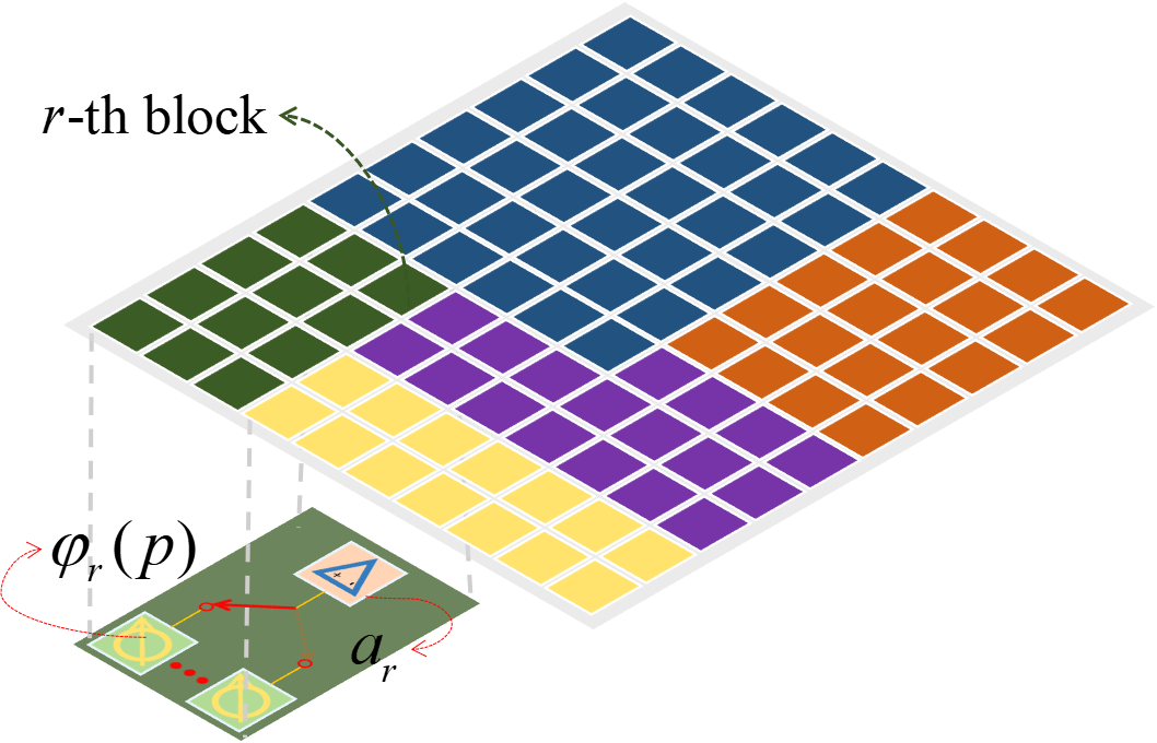
Fig. 2: Block-amplifying architecture of active-ITS.

Note that the variables $\mathbf{U}$, $\mathbf{F}$, $\mathbf{W}$, and $\mathbf{\Theta}$ can be directly obtained as that under element-amplifying architecture case, and hence, the remaining work is to optimize the power amplifying factor matrix, i.e., $\mathbf{A}$, under the block-amplifying architecture case. In the following, we extend the proposed ASO algorithm from the element-wise form into the block-wise form, which can optimize $\mathbf{A}$ in a block-by-block manner.

Remark 2: From a mathematical point of view, since the element-amplifying architecture can be interpreted as a special case ($R=N$) of the block-amplifying architecture, the proposed ASO Algorithm under the block-wise form is a superset of the element-wise form.

Particularly, we partition the power amplifying factor $\mathbf{a}$ into $R$ blocks, i.e., $\mathbf{a}=\left[\mathbf{a}_{1}^{\operatorname{T}},\mathbf{a}_{2}^{\operatorname{T}},\cdots,\mathbf{a}_{R}^{\operatorname{T}}\right]\in\mathbb{R}^{N\times 1}$, where $\mathbf{a}_{r}\in\mathbb{R}^{{\hat{N}}_{r}\times 1}$ is the power amplifying factor vector corresponding to ${\hat{N}}_{r}$ TEs in the $r$-th block, which is given by

$$\mathbf{a}_{r}=\left[{{\mathbf{a}}_{r}\left(1\right),{\mathbf{a}}_{r}\left(2\right),\cdots,{\mathbf{a}}_{r}\left({\hat{N}}_{r}\right)}\right]^{\operatorname{T}}={a}_{r}\bm{1}_{{\hat{N}}_{r}}^{\operatorname{T}},$$ (43)

where $\mathbf{a}_{r}\left({m}\right)$ is the $\left(\sum_{l=1}^{r-1}{{\hat{N}}_{l}}+m\right)$-th element of $\mathbf{a}$ with $r=2,3,\cdots,R$ and $m=1,2,\cdots,{\hat{N}}_{r}$.

Here, let us revisit problem $\mathcal{P}_{4\text{-}1}$ stated in (32). First, $\left(\mathbf{a}^{\operatorname{T}}\circ\bm{\theta}^{\operatorname{H}}\right)\mathbf{\Omega}\left(\mathbf{a}\circ\bm{\theta}\right)$ can be expanded as

$$\left(\mathbf{a}^{\operatorname{T}}\circ\bm{\theta}^{\operatorname{H}}\right)\mathbf{\Omega}\left(\mathbf{a}\circ\bm{\theta}\right)$$

$$= \sum_{i=1,i\neq r}^{R}{\left(\mathbf{a}^{\operatorname{T}}\circ\bm{\theta}^{\operatorname{H}}\right)\bm{\Omega}_{i}\left(\mathbf{a}_{i}\circ\bm{\theta}_{i}\right)}+\left(\mathbf{a}^{\operatorname{T}}\circ\bm{\theta}^{\operatorname{H}}\right)\bm{\Omega}_{r}\left(\mathbf{a}_{r}\circ\bm{\theta}_{r}\right)$$

$$= \sum_{i=1,i\neq r}^{R}{\left(\mathbf{a}_{i}^{\operatorname{T}}\circ\bm{\theta}_{i}^{\operatorname{H}}\right)\bm{\Omega}_{i,r}\left(\mathbf{a}_{r}\circ\bm{\theta}_{r}\right)}+\sum_{i=1,i\neq r}^{R}{\sum_{j=1}^{R}{\left(\mathbf{a}_{j}^{\operatorname{T}}\circ\bm{\theta}_{j}^{\operatorname{H}}\right)\bm{\Omega}_{j,i}\left(\mathbf{a}_{i}\circ\bm{\theta}_{i}\right)}}+\left(\mathbf{a}_{r}^{\operatorname{T}}\circ\bm{\theta}_{r}^{\operatorname{H}}\right)\bm{\Omega}_{r,r}\left(\mathbf{a}_{r}\circ\bm{\theta}_{r}\right),$$

$$= \sum_{i=1,i\neq r}^{R}{\left(\left(\mathbf{a}_{i}^{\operatorname{T}}\circ\bm{\theta}_{i}^{\operatorname{H}}\right)\bm{\Omega}_{i,r}\left(\mathbf{a}_{r}\circ\bm{\theta}_{r}\right)+{\left(\mathbf{a}_{i}^{\operatorname{T}}\circ\bm{\theta}_{i}^{\operatorname{H}}\right)\bm{\Omega}_{i,r}\left(\mathbf{a}_{r}\circ\bm{\theta}_{r}\right)}\right)}$$

$$+\sum_{i=1,i\neq r}^{R}{\sum_{j=1}^{R}{\left(\mathbf{a}_{j}^{\operatorname{T}}\circ\bm{\theta}_{j}^{\operatorname{H}}\right)\bm{\Omega}_{j,i}\left(\mathbf{a}_{i}\circ\bm{\theta}_{i}\right)}}+\left(\mathbf{a}_{r}^{\operatorname{T}}\circ\bm{\theta}_{r}^{\operatorname{H}}\right)\bm{\Omega}_{r,r}\left(\mathbf{a}_{r}\circ\bm{\theta}_{r}\right),$$ (44)

where $\bm{\Omega}=\left[\bm{\Omega}_{1},\bm{\Omega}_{2},\cdots,\bm{\Omega}_{R}\right]$ and $\bm{\theta}=\left[\bm{\theta}_{1}^{\operatorname{T}},\bm{\theta}_{2}^{\operatorname{T}},\cdots,\bm{\theta}_{R}^{\operatorname{T}}\right]^{\operatorname{T}}$, with

$$\bm{\Omega}_{r} =\left[\bm{\Omega}_{1,r},\bm{\Omega}_{2,r},\cdots,\bm{\Omega}_{R,r}\right]^{\operatorname{T}}\in\mathbb{C}^{N\times{\hat{N}}_{r}},$$ (45a)

$$\bm{\theta}_{r} =\left[\bm{\theta}_{r}\left(1\right),\bm{\theta}_{r}\left(2\right),\cdots,\bm{\theta}_{r\left({{\hat{N}}_{r}}\right)}\right]^{\operatorname{T}}\in\mathbb{C}^{{\hat{N}}_{r}\times 1},$$ (45b)

where $\bm{\theta}_{r}\left({m}\right)$ denotes the $\left(\sum_{l=1}^{r-1}{{\hat{N}}_{l}}+m\right)$-th element of $\bm{\theta}$ with $r=2,3,\cdots,R$ and $m=1,2,\cdots,{\hat{N}}_{r}$.

By employing the property $\bm{\Omega}_{i,r}=\bm{\Omega}_{i,r}^{\operatorname{H}}$ , (IV) can be rewritten as

$$\left(\mathbf{a}^{\operatorname{T}}\circ\bm{\theta}^{\operatorname{H}}\right)\mathbf{\Omega}\left(\mathbf{a}\circ\bm{\theta}\right)$$

$$= 2\operatorname{Re}\left\{\sum_{i=1,i\neq r}^{R}{\left(\mathbf{a}_{i}^{\operatorname{T}}\circ\bm{\theta}_{i}^{\operatorname{H}}\right)\bm{\Omega}_{i,r}\left(\mathbf{a}_{r}\circ\bm{\theta}_{r}\right)}\right\}+\sum_{i=1,i\neq r}^{R}{\sum_{j=1}^{R}{\left(\mathbf{a}_{j}^{\operatorname{T}}\circ\bm{\theta}_{j}^{\operatorname{H}}\right)\bm{\Omega}_{j,i}\left(\mathbf{a}_{i}\circ\bm{\theta}_{i}\right)}}$$

$$+\left(\mathbf{a}_{r}^{\operatorname{T}}\circ\bm{\theta}_{r}^{\operatorname{H}}\right)\bm{\Omega}_{r,r}\left(\mathbf{a}_{r}\circ\bm{\theta}_{r}\right).$$ (46)

Then, note that the term $\sum_{i=1,i\neq r}^{R}{\left(\mathbf{a}_{i}^{\operatorname{T}}\circ\bm{\theta}_{i}^{\operatorname{H}}\right)\bm{\Omega}_{i,r}\left(\mathbf{a}_{r}\circ\bm{\theta}_{r}\right)}$ in (IV) can be expanded by

$$\sum_{i=1,i\neq r}^{R}{\left(\mathbf{a}_{i}^{\operatorname{T}}\circ\bm{\theta}_{i}^{\operatorname{H}}\right)\bm{\Omega}_{i,r}\left(\mathbf{a}_{r}\circ\bm{\theta}_{r}\right)}= \sum_{i=1,i\neq r}^{R}{a_{r}a_{i}\left(\bm{1}_{{\hat{N}}_{r}}^{\operatorname{T}}\circ\bm{\theta}_{r}^{\operatorname{H}}\right)\bm{\Omega}_{r,i}\left(\bm{1}_{{\hat{N}}_{i}}\circ\bm{\theta}_{i}\right)}$$

$$= \sum_{i=1,i\neq r}^{R}{a_{r}a_{i}\bm{\theta}_{r}^{\operatorname{H}}\bm{\Omega}_{r,i}\bm{\theta}_{i}}.$$ (47)

Similarly, we have

$$\left(\mathbf{a}_{r}^{\operatorname{T}}\circ\bm{\theta}_{r}^{\operatorname{H}}\right)\bm{\Omega}_{r,r}\left(\mathbf{a}_{r}\circ\bm{\theta}_{r}\right) =a_{r}^{2}\bm{\theta}_{r}^{\operatorname{H}}\bm{\Omega}_{r,r}\bm{\theta}_{r},$$ (48a)

$$\left(\mathbf{a}^{\operatorname{T}}\circ\bm{\theta}^{\operatorname{H}}\right)\mathbf{c} =a_{r}\bm{\theta}_{r}^{\operatorname{H}}\mathbf{c}_{r}+\sum\nolimits_{i=1,i\neq r}^{R}{a_{i}\bm{\theta}_{i}^{\operatorname{H}}\mathbf{c}_{i}}.$$ (48b)

By defining $\mathbf{d}=\operatorname{Vecd}\left(\mathbf{D}\right)$ and $\mathbf{t}=\operatorname{Vecd}\left(\mathbf{T}\right)$, and then partition the two vector into $R$ blocks, i.e., $\mathbf{d}=\left[\mathbf{d}_{1}^{\operatorname{T}},\mathbf{d}_{2}^{\operatorname{T}},\cdots,\mathbf{d}_{R}^{\operatorname{T}}\right]\in\mathbb{C}^{N\times 1}$ and $\mathbf{t}=\left[\mathbf{t}_{1}^{\operatorname{T}},\mathbf{t}_{2}^{\operatorname{T}},\cdots,\mathbf{t}_{R}^{\operatorname{T}}\right]\in\mathbb{C}^{N\times 1}$, we have

$$\operatorname{Tr}\left(\bm{\Phi}^{\operatorname{H}}\mathbf{D}\bm{\Phi}\right) =a_{r}^{2}\sum_{p=1}^{{\hat{N}}_{r}}{\mathbf{d}_{r}\left(p\right)}+\sum_{i=1,i\neq r}^{R}{a_{i}^{2}\sum_{q=1}^{{\hat{N}}_{i}}{\mathbf{d}_{i}\left(q\right)}},$$ (49a)

$$\operatorname{Tr}\left(\bm{\Phi}^{\operatorname{H}}\bm{\Phi}\mathbf{T}\right) =a_{r}^{2}\sum_{p=1}^{{\hat{N}}_{r}}{\mathbf{t}_{r}\left(p\right)}+\sum_{i=1,i\neq r}^{R}{a_{i}^{2}\sum_{q=1}^{{\hat{N}}_{i}}{\mathbf{t}_{i}\left(q\right)}}.$$ (49b)

Similarly, we have

$$\operatorname{Tr}\left(\bm{\Phi}^{\operatorname{H}}\bm{\Phi}\right) =a_{r}^{2}{\hat{N}}_{r}+\sum\nolimits_{i=1,i\neq r}^{R}{a_{i}^{2}{{\hat{N}}_{i}}}.$$ (50)

Consequently, problem $\mathcal{P}_{4\text{-}1}$ can be reformulated by

$$\mathcal{P}_{5}:\mathop{\min}_{a_{r}}\; f\left(a_{r}\right)=a_{r}^{2}m_{r}+2\operatorname{Re}\left\{a_{r}z_{r}\right\}+\chi_{r},$$ (51a)

$$\operatorname{s.t.}\; a_{r}^{2}g_{r}\leq{\hat{P}}_{\operatorname{ITS}}^{\max},$$ (51b)

where

$$m_{r} =\bm{\theta}_{r}^{\operatorname{H}}\bm{\Omega}_{r,r}\bm{\theta}_{r}+\delta^{2}\kappa^{2}\sum_{p=1}^{{\hat{N}}_{r}}{\mathbf{d}_{r}\left(p\right)},$$ (52a)

$$z_{r} =\sum_{i=1,i\neq r}^{R}{a_{i}\bm{\theta}_{r}^{\operatorname{H}}\bm{\Omega}_{r,i}\bm{\theta}_{i}}-\bm{\theta}_{r}^{\operatorname{H}}\mathbf{c}_{r},$$ (52b)

$$g_{r} =\sum_{p=1}^{{\hat{N}}_{r}}{\mathbf{t}_{r}\left(p\right)}+\kappa^{2}\delta^{2}{\hat{N}}_{r},$$ (52c)

$${\hat{P}}_{\operatorname{ITS}}^{\max} =P_{\operatorname{ITS}}^{\max}-\sum_{i=1,i\neq r}^{R}{a_{i}^{2}\sum_{q=1}^{{\hat{N}}_{i}}{\mathbf{t}_{i}\left(q\right)}}-\kappa^{2}\delta^{2}\sum_{i=1,i\neq r}^{R}{a_{i}^{2}{{\hat{N}}_{i}}},$$ (52d)

and where $\chi_{r}$ denotes a constant value with respect to $a_{r}$ and does not affect its solution, and is given by

$$\chi_{r}=\sum_{i=1,i\neq r}^{R}{\sum_{j=1}^{R}{a_{j}a_{i}\bm{\theta}_{j}^{\operatorname{H}}\bm{\Omega}_{j,i}\bm{\theta}_{i}}}+2\operatorname{Re}\left\{\sum_{i=1,i\neq r}^{R}{a_{i}\bm{\theta}_{i}^{\operatorname{H}}\mathbf{c}_{i}}\right\}+\kappa^{2}\delta^{2}\sum_{i=1,i\neq r}^{R}{a_{i}^{2}\sum_{q=1}^{{\hat{N}}_{i}}{\mathbf{d}_{i}\left(q\right)}}.$$ (53)

The above problem can be solved similarly to (42) and hence it is omitted for brevity.

Based on the above discussions, $\mathbf{a}_{r},\forall r$ can be conducted by successively optimizing with the other $R-1$ blocks being fixed, and then repeat until the convergence is attained [51].

V Simulation Result

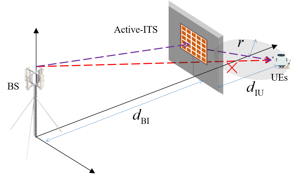
Fig. 3: The simulated active-ITS empowered outdoor-to-indoor mmWave communication.

In this section, numerical results are provided to evaluate the WSR performance achieved by the proposed BCD-based joint precoding algorithm under the two architectures of active-ITSs.

V-A Simulation Setup

We consider a three-dimensional setup as illustrated in Fig. 3, where the BS at the outdoor communicates with UEs at the indoor with the aid of an active-ITS. The BS, active-ITS, and UEs are assumed in a straight line, and heights of them are 3m, 6m, and 1.5m, respectively, and the total horizontal distances $d_{\text{BU}}=d_{\text{BI}}+d_{\text{IU}}=50$ m. The $K=4$ UEs are uniformly and randomly distributed in a circle centered at $(0\operatorname{m},50\operatorname{m})$ with a radius of $5$ m.

For array response vector, the azimuth angles of arrival $\upsilon^{\operatorname{AOA}}$ and departure $\upsilon^{\operatorname{AOD}}$ are uniformly distributed in the interval $\left[-\pi,\pi\right)$. The elevation angles of arrival $\vartheta^{\operatorname{AOA}}$ and departure $\vartheta^{\operatorname{AOD}}$ are uniformly distributed in the interval $\left[-\pi/2,\pi/2\right)$. The complex gains of LOS paths $\alpha_{l},\forall l$ and $\beta_{p},\forall p$ are independently distributed with $\mathcal{C}\mathcal{N}\left(0,10^{-0.1{\operatorname{PL}}}\right)$, where the distance-dependent path loss $\operatorname{PL}$ for both the LoS and the NLoS paths can be modeled by

$$\operatorname{PL}=\operatorname{PL_{0}}+10b\log_{10}\left(D\right)+\zeta\,\text{dB},$$ (54)

where $D$ denotes the individual link distance and $\zeta$ denotes lognormal shadow fading following $\zeta\sim\mathcal{N}\left(0,\sigma_{\zeta}^{2}\right)$. As the real-world channel measurements for the carrier frequency of 28 GHz suggested in [3, Table I], the values of the parameters in (54) are set as $\operatorname{PL_{0}}=61.4$, $b=2$, and $\sigma_{\zeta}=5.8$ dB for the LoS paths, and $\operatorname{PL_{0}}=72$, $b=2.92$, and $\sigma_{\zeta}=8.7$ dB for NLoS paths. The bandwidth $B=251$ MHz, the noise power is $\sigma^{2}=-174+10\log_{10}B=-90$ dBm. Unless otherwise stated, the other adopted simulation parameters are set as follows: the distance between the BS and ITS of $d_{\operatorname{BI}}=45$ m, the circuit power consumption for phase-shifting and power-amplifying are $P_{\operatorname{SW}}=-10$ dBm and $P_{\operatorname{DC}}=-5$ dBm [34], the power budgets of the BS and active-ITS are $P_{\operatorname{BS}}^{\max}=30$ dBm and $P_{\operatorname{ITS}}^{\max}=30$ dBm, the number of TEs of $N=10\times 4$, the number of antennas of $M_{t}=4\times 2$ and $M_{r}=2\times 2$, the weighting factor of $\alpha_{k}=1,\forall k$, the penetration efficiency of $\kappa=0.8$, and the target accuracy of $\varepsilon=10^{-3}$.

Without loss of generality, for the block-amplifying ITS architecture, we adopt an evenly-block strategy, where the number of TEs in each block is equal and set as 5 and 10, i.e., “Block-amplifying ITS, $N_{B}=5$” and “Block-amplifying ITS, $N_{B}=10$”. We also introduce a baseline scheme “Block-amplifying ITS, $N_{B}=N$”, where all TEs of ITS share the same power amplifier, so all the active TEs have identical amplitudes, i.e., $a_{n}=a,\forall n\in N$ [36]. In addition, due to that the active-ITS requires an additional power, i.e., $P_{\operatorname{ITS}}^{\max}$, and hence, for fair comparisons, we assume that the power budget at the BS for the passive-ITS scheme (referred as “Without-amplifying ITS”) is allocated an additional amount of $P_{\operatorname{ITS}}^{\max}$, i.e., $P_{\operatorname{BS,passive}}^{\max}=P_{\operatorname{ITS}}^{\max}+P_{\operatorname{BS,active}}^{\max}$, so that all the compared schemes have the same total power consumption.

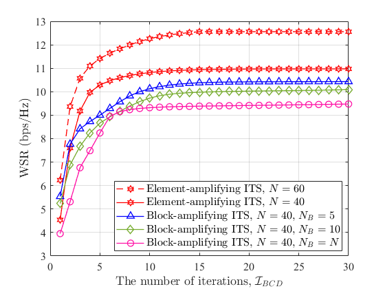
Fig. 4: WSR against the number of iterations, $\mathcal{I}_{BCD}$.

V-B Convergence Behavior

In this subsection, we investigate the convergence behavior of the proposed BCD-based algorithm for the different architectures of active-ITSs with different numbers of TEs. As shown in Fig. 4, we plot the curves of the WSR performance achieved by the proposed algorithm for the active-ITS schemes (include Element-amplifying ITS and Block-amplifying ITS) against the number of iterations. In particular, it can be observed that the curve with $N=60$ TEs converges slower than that of $N=40$ TEs, and the curves of both the element-amplifying architecture and the block-amplifying architecture converge to corresponding stationary points after a few iterations. The observation is consistent with our expectations. It can be concluded that the proposed algorithm has good convergence behavior and the convergence speed is sensitive to the number of TEs of an active-ITS, and the impact of $N_{B}$ on the convergence speed is slight.

V-C The impact of key parameters on WSR performances

In this subsection, we study the WSR performance achieved by the proposed algorithms for both the active-ITS scheme and the passive-ITS scheme (i.e., Without-amplifying ITS) versus the key parameters of the considered system setting. All the simulation results as follows are averaged over 1,000 independent channel realizations.

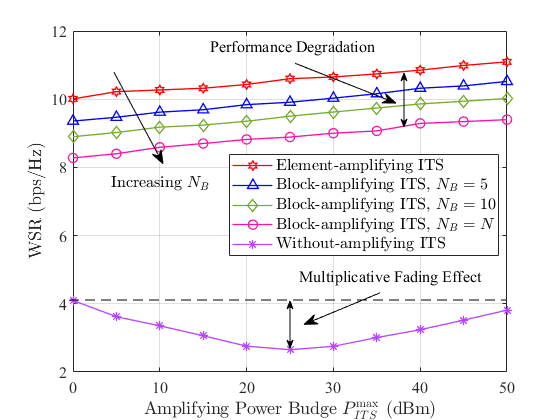
Fig. 5: WSR against the position of the active-ITS, $d_{\operatorname{BI}}$.

In Fig. 5, we investigate the WSR performance for different locations of the ITS by varying the distance between the BS and ITS, i.e., $d_{\operatorname{BI}}$. One important observation is that with increasing $d_{\operatorname{BI}}$, the WSR performance achieved by the active-ITS scheme monotonically increase, which is different from the passive-ITS scheme, which achieve the highest and the worst WSR performances when passive-ITS are deployed close to the BS(UEs) and at the middle location due to the multiplicative fading effect. This interesting observation indicates that the active-ITS should to be deployed closer to UEs for fully unleashing its potential on achieving a better WSR performance. Intuitively speaking, the deployment strategy meets the requirements of a practical outdoor-to-indoor communication scenario where the active-ITS is usually very close to the UEs, i.e., $d_{\operatorname{IU}}\ll d_{\operatorname{BI}}$. In addition, it can be observed that the active-ITS schemes perform constantly better than passive-ITS scheme in all locations, which implies that the active-ITS brings a significant performance gain compared with the passive-ITS due to the amplified signal is only attenuated once. More importantly, it can be seen that the WSR of “Element-amplifying ITS” scheme outperforms that of the “Block-amplifying ITS” schemes, which can be attributed to that the block-amplifying architecture of active-ITS inevitably lost some DoF for proactively configuring the wireless channels. This observation indicates the importance of carefully optimizing the power amplification factor matrix at the active-ITS for enhancing the WSR performance. Nevertheless, considering that such a block-amplifying architecture of active-ITS can reduce the scale of the power-amplifying circuit for application to space-limited scenarios, the resulting slight performance gap is acceptable.

The WSR performances versus the number of TEs with $P_{\operatorname{ITS}}^{\max}=30$ dBm and $P_{\operatorname{ITS}}^{\max}=20$ dBm are shown in Fig. 6. It illustrates that with the increasing number of TEs, both curves of the active-ITS and the passive-ITS schemes monotonically increases, since more TEs introduce more DoFs to proactively configure the wireless channel which yields a higher WSR performance. Meanwhile, it also illustrates the superiority of the active-ITS that brings a large benefit to WSR performance compared with the passive-ITS. Particularly, the usage of active ITSs can greatly reduce the number of TEs compared with passive ITS case for reaping a given performance level, and hence greatly decrease both the size and the complexity of ITS, which is beneficial for embedding in space-limited and aesthetic-needed building structures. It can be explained by that when equipped a small number of active TEs in the active-ITS, according to the constraint in (9c), a larger power amplification factor will be allocated at each active TE. In addition, it can be observed that with a small number of TEs, the performance degradation between element-amplifying ITS and block-amplifying ITS is slight with $P_{\operatorname{ITS}}^{\max}=20$ dBm, while the performance gap in the large $N$ regime also is acceptable. This observation is because that for a large number of TEs at the active-ITS, the block-amplifying architecture has more power to amplify the signal, which can compensate for some of the loss of performance. This observation highlights the effectiveness of the proposed block-amplifying architecture.

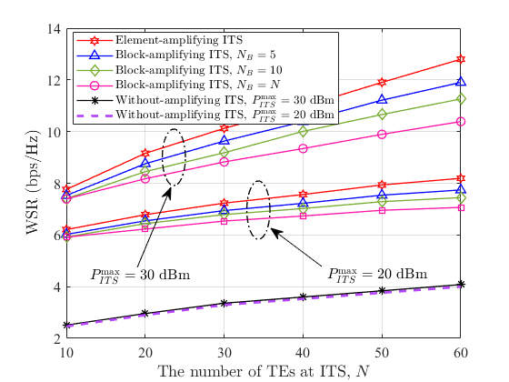
Fig. 6: WSR against the number of TEs.

We plot the WSR performance against the amplifying power budget at ITS in Fig. 7. As expected, it can be observed that all the WSR performances of all schemes increase as $P_{\operatorname{ITS}}^{\max}$ increase. More specifically, the WSR performances achieved by the active-ITS schemes outperform that of passive-ITS, which indicates that the active-ITS can exploit a part of the power for fighting with the multiplicative path loss effect influence and achieving a higher WSR performance than the passive-ITS scheme for the same power consumption. In addition, it can be concluded from Fig. 7 that the active-ITS scheme can significantly reduce the power consumption compared to the passive-ITS scheme when achieving a given performance level. More importantly, it can be observed that the performance degradation caused by the block-amplifying architecture of the active-ITS is slight when $P_{ITS}^{\max}=15$ dBm, which is because that the more power is used for the circuit static power consumption in the small $P_{ITS}^{\max}$ regime.

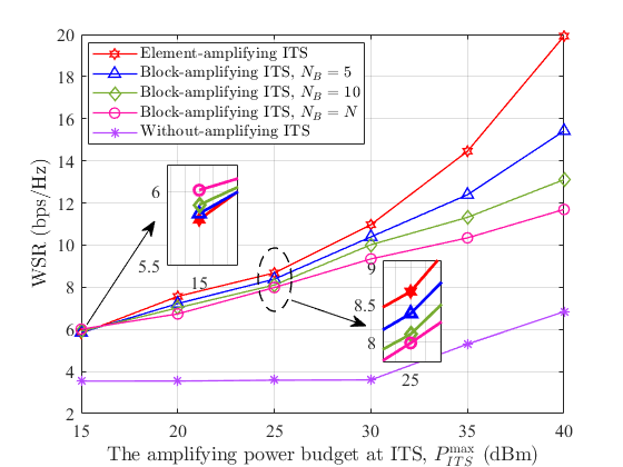
Fig. 7: WSR against the amplifying power budget $P_{\operatorname{ITS}}^{\max}$ at the active-ITS.

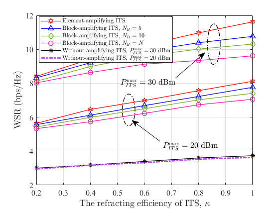
Fig. 8: WSR against the refracting efficiency $\kappa$.

Fig. 8 illustrates the WSR performance against the refracting efficiency of ITSs. It can be observed that the refracting efficiency of ITS has a substantial impact on the WSR performance, whereas expected, with the increasing $\kappa$, the WSR achieved by the active-ITS schemes increased significantly. The refracting efficiency of an ITS is determined by the hardware components, which is used to characterize the power loss caused by signal absorption and signal reflection when the mmWave signal impinges upon and penetrate the ITS. This figure demonstrates the benefits of active-ITS that can exploit the additional power amplifiers to compensate for the power loss caused by the practical hardware component.

VI Conclusion

In this paper, an active-ITS empowered outdoor-to-indoor mmWave communication system was investigated, where the active-ITS benefited on greatly reducing the number of TEs while maintaining a given performance compared with the passive-ITS. To jointly optimize the linear precoding matrix of the BS and transmissive coefficients of the active-ITS, we formulated a WSR maximization problem, and then a BCD-based joint precoding algorithm was proposed for solving it. In order to further reduce the size and hardware cost of active-ITS, a block-amplifying architecture was proposed to partially remove the hardware components for power amplifying. And then we extended the proposed BCD-based joint precoding algorithm into the block-wise form for optimizing the transmissive coefficients of the active-ITS under the block-amplifying architecture. Simulation results demonstrated that the active-ITS could significantly enhance the system performance, and the inevitable performance degradation caused by the block-amplifying ITS architecture was acceptable.

References

• [1] R. W. Heath, N. González-Prelcic, S. Rangan, W. Roh, and A. M. Sayeed, “An Overview of Signal Processing Techniques for Millimeter Wave MIMO Systems,” IEEE Journal of Selected Topics in Signal Processing, vol. 10, no. 3, pp. 436–453, Apr. 2016.
• [2] M. Di Renzo, “Stochastic Geometry Modeling and Analysis of Multi-Tier Millimeter Wave Cellular Networks,” IEEE Transactions on Wireless Communications, vol. 14, no. 9, pp. 5038–5057, Sep. 2015.
• [3] M. R. Akdeniz, Y. Liu, M. K. Samimi, S. Sun, S. Rangan, T. S. Rappaport, and E. Erkip, “Millimeter Wave Channel Modeling and Cellular Capacity Evaluation,” IEEE Journal on Selected Areas in Communications, vol. 32, no. 6, pp. 1164–1179, Jun. 2014.
• [4] X. Hu, C. Zhong, Y. Zhu, X. Chen, and Z. Zhang, “Programmable Metasurface-Based Multicast Systems: Design and Analysis,” IEEE Journal on Selected Areas in Communications, vol. 38, no. 8, pp. 1763–1776, Aug. 2020.
• [5] M. A. ElMossallamy, H. Zhang, L. Song, K. G. Seddik, Z. Han, and G. Y. Li, “Reconfigurable Intelligent Surfaces for Wireless Communications: Principles, Challenges, and Opportunities,” IEEE Transactions on Cognitive Communications and Networking, vol. 6, no. 3, pp. 990–1002, Sep. 2020.
• [6] M. Di Renzo, A. Zappone, M. Debbah, M. S. Alouini, C. Yuen, J. de Rosny, and S. Tretyakov, “Smart Radio Environments Empowered by Reconfigurable Intelligent Surfaces: How It Works, State of Research, and The Road Ahead,” IEEE Journal on Selected Areas in Communications, vol. 38, no. 11, pp. 2450–2525, Nov. 2020.
• [7] G. Zhou, C. Pan, H. Ren, K. Wang, M. Elkashlan, and M. D. Renzo, “Stochastic Learning-Based Robust Beamforming Design for RIS-Aided Millimeter-Wave Systems in the Presence of Random Blockages,” IEEE Transactions on Vehicular Technology, vol. 70, no. 1, pp. 1057–1061, Jan. 2021.
• [8] P. Wang, J. Fang, L. Dai, and H. Li, “Joint Transceiver and Large Intelligent Surface Design for Massive MIMO mmWave Systems,” IEEE Transactions on Wireless Communications, vol. 20, no. 2, pp. 1052–1064, Feb. 2021.
• [9] Y. Chen, Y. Wang, and L. Jiao, “Robust Transmission for Reconfigurable Intelligent Surface Aided Millimeter Wave Vehicular Communications With Statistical CSI,” IEEE Transactions on Wireless Communications, vol. 21, no. 2, pp. 928–944, Feb. 2022.
• [10] Y. Xiu, J. Zhao, E. Basar, M. D. Renzo, W. Sun, G. Gui, and N. Wei, “Uplink Achievable Rate Maximization for Reconfigurable Intelligent Surface Aided Millimeter Wave Systems With Resolution-Adaptive ADCs,” IEEE Wireless Communications Letters, vol. 10, no. 8, pp. 1608–1612, Aug. 2021.
• [11] H. Niu, Z. Chu, F. Zhou, C. Pan, D. W. K. Ng, and H. X. Nguyen, “Double Intelligent Reflecting Surface-Assisted Multi-User MIMO Mmwave Systems With Hybrid Precoding,” IEEE Transactions on Vehicular Technology, vol. 71, no. 2, pp. 1575–1587, Feb. 2022.
• [12] C. Feng, W. Shen, J. An, and L. Hanzo, “Joint Hybrid and Passive RIS-Assisted Beamforming for MmWave MIMO Systems Relying on Dynamically Configured Subarrays,” IEEE Internet of Things Journal, pp. 1–1, 2022.
• [13] V. Jamali, A. M. Tulino, G. Fischer, R. R. Müller, and R. Schober, “Intelligent Surface-Aided Transmitter Architectures for Millimeter-Wave Ultra Massive MIMO Systems,” IEEE Open Journal of the Communications Society, vol. 2, pp. 144–167, Dec. 2021.
• [14] D. W. K. Ng, M. Breiling, C. Rohde, F. Burkhardt, and R. Schober, “Energy-Efficient 5G Outdoor-to-Indoor Communication: SUDAS Over Licensed and Unlicensed Spectrum,” IEEE Transactions on Wireless Communications, vol. 15, no. 5, pp. 3170–3186, May. 2016.
• [15] H. Zhao, R. Mayzus, S. Sun, M. Samimi, J. K. Schulz, Y. Azar, K. Wang, G. N. Wong, F. Gutierrez, and T. S. Rappaport, “28 GHz Millimeter Wave Cellular Communication Measurements for Reflection and Penetration Loss in and Around Buildings in New York City,” in 2013 IEEE International Conference on Communications (ICC), Jun. 2013, pp. 5163–5167.
• [16] K. Ntontin and C. Verikoukis, “Relay-Aided Outdoor-to-Indoor Communication in Millimeter-Wave Cellular Networks,” IEEE Systems Journal, vol. 14, no. 2, pp. 2473–2484, Jun. 2020.
• [17] M. Nemati, B. Maham, S. R. Pokhrel, and J. Choi, “Modeling RIS Empowered Outdoor-to-Indoor Communication in mmWave Cellular Networks,” IEEE Transactions on Communications, vol. 69, no. 11, pp. 7837–7850, Nov. 2021.
• [18] Q. Wu and R. Zhang, “Beamforming Optimization for Wireless Network Aided by Intelligent Reflecting Surface With Discrete Phase Shifts,” IEEE Transactions on Communications, vol. 68, no. 3, pp. 1838–1851, Mar. 2020.
• [19] E. Basar and H. V. Poor, “Present and Future of Reconfigurable Intelligent Surface-Empowered Communications [Perspectives],” IEEE Signal Processing Magazine, vol. 38, no. 6, pp. 146–152, Nov. 2021.
• [20] W. Mei and R. Zhang, “Distributed Beam Training for Intelligent Reflecting Surface Enabled Multi-Hop Routing,” IEEE Wireless Communications Letters, vol. 10, no. 11, pp. 2489–2493, Nov. 2021.
• [21] B. Zheng, C. You, and R. Zhang, “Double-IRS Assisted Multi-User MIMO: Cooperative Passive Beamforming Design,” IEEE Transactions on Wireless Communications, vol. 20, no. 7, pp. 4513–4526, Jul. 2021.
• [22] S. Zeng, H. Zhang, B. Di, Y. Tan, Z. Han, H. V. Poor, and L. Song, “Reconfigurable Intelligent Surfaces in 6G: Reflective, Transmissive, or Both?” IEEE Communications Letters, vol. 25, no. 6, pp. 2063–2067, Jun. 2021.
• [23] K. Liu, Z. Zhang, L. Dai, and L. Hanzo, “Compact User-Specific Reconfigurable Intelligent Surfaces for Uplink Transmission,” IEEE Transactions on Communications, vol. 70, no. 1, pp. 680–692, Jan. 2022.
• [24] N. Landsberg and E. Socher, “Design and Measurements of 100 GHz Reflectarray and Transmitarray Active Antenna Cells,” IEEE Transactions on Antennas and Propagation, vol. 65, no. 12, pp. 6986–6997, Dec. 2017.
• [25] C. Pfeiffer and A. Grbic, “Metamaterial Huygens’ Surfaces: Tailoring Wave Fronts with Reflectionless Sheets,” Physical Review Letters, vol. 110, no. 19, pp. 197 401–197 401, May. 2013.
• [26] Y. Liu, X. Mu, J. Xu, R. Schober, Y. Hao, H. V. Poor, and L. Hanzo, “STAR: Simultaneous Transmission and Reflection for 360° Coverage by Intelligent Surfaces,” IEEE Wireless Communications, vol. 28, no. 6, pp. 102–109, Dec. 2021.
• [27] M. Aldababsa, A. Khaleel, and E. Basar, “Simultaneous Transmitting and ReflectingIntelligent Surfaces-Empowered NOMA Networks,” arXiv preprint arXiv:2110.05311, 2021.
• [28] X. Mu, Y. Liu, L. Guo, J. Lin, and R. Schober, “Simultaneously Transmitting And Reflecting (STAR) RIS Aided Wireless Communications,” IEEE Transactions on Wireless Communications, vol. 21, no. 5, pp. 3083–3098, 2022.
• [29] S. Zhang, H. Zhang, B. Di, Y. Tan, M. Di Renzo, Z. Han, H. Vincent Poor, and L. Song, “Intelligent Omni-Surfaces: Ubiquitous Wireless Transmission by Reflective-Refractive Metasurfaces,” IEEE Transactions on Wireless Communications, vol. 21, no. 1, pp. 219–233, Jan. 2022.
• [30] Z. Zhang, L. Dai, X. Chen, C. Liu, F. Yang, R. Schober, and H. V. Poor, “Active RIS vs. passive RIS: Which will prevail in 6G?” arXiv preprint arXiv:2103.15154, 2021.
• [31] S. Zhang and R. Zhang, “Intelligent Reflecting Surface Aided Multi-User Communication: Capacity Region and Deployment Strategy,” IEEE Transactions on Communications, vol. 69, no. 9, pp. 5790–5806, Sep. 2021.
• [32] L. Dong, H.-M. Wang, and J. Bai, “Active Reconfigurable Intelligent Surface Aided Secure Transmission,” IEEE Transactions on Vehicular Technology, vol. 71, no. 2, pp. 2181–2186, Feb. 2022.
• [33] D. Xu, X. Yu, D. W. Kwan Ng, and R. Schober, “Resource Allocation for Active IRS-Assisted Multiuser Communication Systems,” in 2021 55th Asilomar Conference on Signals, Systems, and Computers, Oct. 2021, pp. 113–119.
• [34] R. Long, Y.-C. Liang, Y. Pei, and E. G. Larsson, “Active Reconfigurable Intelligent Surface-Aided Wireless Communications,” IEEE Transactions on Wireless Communications, vol. 20, no. 8, pp. 4962–4975, Aug. 2021.
• [35] M. H. Khoshafa, T. M. N. Ngatched, M. H. Ahmed, and A. R. Ndjiongue, “Active Reconfigurable Intelligent Surfaces-Aided Wireless Communication System,” IEEE Communications Letters, vol. 25, no. 11, pp. 3699–3703, Sep. 2021.
• [36] K. Zhi, C. Pan, H. Ren, K. K. Chai, and M. Elkashlan, “Active RIS Versus Passive RIS: Which Is Superior with the Same Power Budget?” IEEE Communications Letters, vol. 26, no. 5, pp. 1150–1154, 2022.
• [37] C. You and R. Zhang, “Wireless Communication Aided by Intelligent Reflecting Surface: Active or Passive?” IEEE Wireless Communications Letters, vol. 10, no. 12, pp. 2659–2663, Dec. 2021.
• [38] R. A. Tasci, F. Kilinc, E. Basar, and G. C. Alexandropoulos, “An Amplifying RIS Architecture with a Single Power Amplifier: Energy Efficiency and Error Performance Analysis,” arXiv preprint arXiv:2111.09855, 2021.
• [39] N. T. Nguyen, D. Vu, K. Lee, and M. Juntti, “Hybrid Relay-Reflecting Intelligent Surface-Assisted Wireless Communications,” IEEE Transactions on Vehicular Technology, pp. 1–1, 2022.
• [40] X. Ying, U. Demirhan, and A. Alkhateeb, “Relay Aided Intelligent Reconfigurable Surfaces: Achieving the Potential Without So Many Antennas,” CoRR, vol. abs/2006.06644, 2020. [Online]. Available: https://arxiv.org/abs/2006.06644
• [41] C. Pan, H. Ren, K. Wang, W. Xu, M. Elkashlan, A. Nallanathan, and L. Hanzo, “Multicell MIMO Communications Relying on Intelligent Reflecting Surfaces,” IEEE Transactions on Wireless Communications, vol. 19, no. 8, pp. 5218–5233, Aug. 2020.
• [42] M. Hua, Q. Wu, D. W. K. Ng, J. Zhao, and L. Yang, “Intelligent Reflecting Surface-Aided Joint Processing Coordinated Multipoint Transmission,” IEEE Transactions on Communications, vol. 69, no. 3, pp. 1650–1665, Mar. 2021.
• [43] X. Xie, C. He, H. Luan, Y. Dong, K. Yang, F. Gao, and Z. J. Wang, “A Joint Optimization Framework for IRS-assisted Energy Self-sustainable IoT Networks,” IEEE Internet of Things Journal, pp. 1–1, 2022.
• [44] M.-M. Zhao, Q. Wu, M.-J. Zhao, and R. Zhang, “Exploiting Amplitude Control in Intelligent Reflecting Surface Aided Wireless Communication With Imperfect CSI,” IEEE Transactions on Communications, vol. 69, no. 6, pp. 4216–4231, Jun. 2021.
• [45] Q. Shi, M. Razaviyayn, Z. Luo, and C. He, “An Iteratively Weighted MMSE Approach to Distributed Sum-Utility Maximization for a MIMO Interfering Broadcast Channel,” IEEE Transactions on Signal Processing, vol. 59, no. 9, pp. 4331–4340, Sep. 2011.
• [46] M. Grant and S. Boyd, “CVX: Matlab Software for Disciplined Convex Programming, Version 2.1,” http://cvxr.com/cvx, Mar. 2014.
• [47] L. Zhang, R. Zhang, Y.-C. Liang, Y. Xin, and H. V. Poor, “On Gaussian MIMO BC-MAC Duality With Multiple Transmit Covariance Constraints,” IEEE Transactions on Information Theory, vol. 58, no. 4, pp. 2064–2078, Apr. 2012.
• [48] X. Zhang, Matrix Analysis and Applications.   Cambridge University Press, 2017.
• [49] C. Pan, H. Ren, K. Wang, M. Elkashlan, A. Nallanathan, J. Wang, and L. Hanzo, “Intelligent Reflecting Surface Aided MIMO Broadcasting for Simultaneous Wireless Information and Power Transfer,” IEEE Journal on Selected Areas in Communications, vol. 38, no. 8, pp. 1719–1734, Jun 2020.
• [50] S. Zhang and R. Zhang, “Capacity Characterization for Intelligent Reflecting Surface Aided MIMO Communication,” IEEE Journal on Selected Areas in Communications, vol. 38, no. 8, pp. 1823–1838, Aug. 2020.
• [51] G. Cui, X. Yu, G. Foglia, Y. Huang, and J. Li, “Quadratic Optimization With Similarity Constraint for Unimodular Sequence Synthesis,” IEEE Transactions on Signal Processing, vol. 65, no. 18, pp. 4756–4769, Sep. 2017.