Fewest-Switches Surface Hopping with Long Short-Term Memory Networks

Abstract

The mixed quantum-classical dynamical simulation is essential to study nonadiabatic phenomena in photophysics and photochemistry. In recent years, many machine learning models have been developed to accelerate the time evolution of the nuclear subsystem. Herein, we implement long short-term memory (LSTM) networks as a propagator to accelerate the time evolution of the electronic subsystem during the fewest-switches surface hopping (FSSH) simulations. A small number of reference trajectories are generated using the original FSSH method, and then the LSTM networks can be built, accompanied by careful examination of typical LSTM-FSSH trajectories that employ the same initial condition and random numbers as the corresponding reference. The constructed network is applied to FSSH to further produce a trajectory ensemble to reveal the mechanism of nonadiabatic processes. Taking Tully’s three models as test systems, the collective results can be reproduced qualitatively. This work demonstrates that LSTM is applicable to the most popular surface hopping simulations.

Yantai-Jingshi Institute of Material Genome Engineering, Yantai 265505 Shandong, China Yantai-Jingshi Institute of Material Genome Engineering, Yantai 265505 Shandong, China

TOC graphic

Dynamical simulations governed by the laws of quantum mechanics are indispensable for providing intuitive views of photophysical and photochemical processes.^{1, 2, 3} Although a fully quantum treatment on both nuclear and electronic motion should be employed in principle, such a simulation is too computationally expensive for medium-sized or larger polyatomic molecules. The requirement of prior knowledge about potential energy surface (PES) further hampers its application on realistic molecular systems with high dimensionality. As an alternative, the mixed quantum-classical molecular dynamics (MQC-MD) approach provides a powerful tool to study the mechanism of photochemical reactions, including the excited-state lifetimes and the quantum yields of photoproducts on different reaction channels. During MQC-MD simulations, the nuclei are represented as classical particles but incorporate quantum feedback from the electronic motion. Many theoretical models and algorithms for MQC-MD have been developed over the past decades.^{4, 5, 6, 7, 8, 9} The most popular method is the fewest-switches surface hopping (FSSH)^{10, 11}, in which the nuclei travel classically on a single PES in an adiabatic electronic state with a probability of switching to any other state. The hopping probability is extracted from the time evolution of electronic degrees of freedom. Despite its simplicity for implementation and great success in many applications^{12, 13, 14}, the computational cost on FSSH is still much more expensive than ground-state MD, especially with the growing demand of simulations on photodynamics in long timescale.¹⁵ At each time step, electronic structure calculations on ground and excited electronic states, including potential energies, gradients as well as nonadiabatic coupling vectors (NACVs) between different states, are usually required at a high level of theory. How to accelerate dynamical simulations remains an important topic if we are willing to extend FSSH to a broader prospect.

In recent years, we have witnessed the prosperity of machine learning (ML) assisted chemical researches.^{16, 17, 18, 19, 20} Several ML techniques such as kernel ridge regression and artificial neural network have been proved as promising tools to provide a relation between molecular structure and ground-state potential energy, so-called ML-based PES or ML-based force field.^{21, 22, 23, 24, 25, 26, 27, 28} Because of its great potential to achieve high computational accuracy and high efficiency on MD simulations simultaneously, the extension to MQC-MD is attractive and seems to be straightforward. In principle, each of adiabatic PESs can be individually fitted as the same as the proposed ML-based force fields. However, the nonadiabatic coupling vectors between adiabatic states have become a challenge for a fully ML-based MQC-MD simulations. One solution is based on the Landau-Zener formalism such as Zhu-Nakamura dynamics^{29, 30}, in which the probability of surface hopping can be obtained only from adiabatic energies and gradients, without the need to compute NACVs. It has been successfully applied to ML-based nonadiabatic molecular dynamics approaches recently^{31, 32}, but the limitation of Landau-Zener formalism as well as its influence on final simulation results is not easy to realize or control. Another way is to improve ML models to fit the reference values of NACVs.^{33, 34, 35, 36} Despite its success on some systems, it is worthy noting that machine learning on nonadiabatic coupling is a nontrivial issue for high-dimensional molecules because NACV keeps almost negligible in most regions of PES but becomes very sensitive to small changes of nuclear positions in the vicinity of conical intersections. The construction on a high-quality ML database is also extremely time-consuming in practice on account of multi-configuration electronic structure calculations for accurate reference values.

In the above approaches, machine learning models are developed and applied to predict potential energies, gradients and nonadiabatic coupling vectors instead of electronic structure calculations, while the time evolution of nuclei and electrons is still governed by the Newton’s second law and the time-dependent Schrödinger equation, respectively. A time series of nuclear positions, velocities and elements of electronic density matrix is obtained and updated during simulations. It suggests employing machine learning to propagate nuclear and/or electronic subsystems based on historical knowledge extracted from the preceding trajectory data. On one hand, ML techniques such as recurrent neural network (RNN) and long short-term memory (LSTM) network have been introduced to classical MD for realistic material and protein systems to solve Newton’s equations.^{37, 38, 39, 40} On the other hand, several successful ML applications on quantum dynamics have been also proposed in recent years.^{41, 42, 43} For example, Lan and coworkers simulated electronic evolution of multi-configuration time-dependent hartree method with LSTM;⁴⁴ Ullah and Dral studied quantum dissipative dynamics of spin-boson model and Fenna-Matthews-Olson complex using kernel ridge regression and convolutional neural network, respectively;^{45, 46} Hammes-Schiffer and coworkers employed artificial neural networks to solve the time-dependent Schrödinger equation and propagate the wavepacket relevant to proton transfer systems.⁴⁷ There are also reports of deep learning in prediction of Landau-Zener transitions^{48, 49} as well as linearized semiclassical and symmetrical quasiclassical mapping dynamics⁵⁰. This inspired of us that machine learning can be implemented as propagator for electronic degrees of freedom in mixed quantum-classical molecular dynamics, possibly avoiding expensive computation or difficult prediction on NACVs.

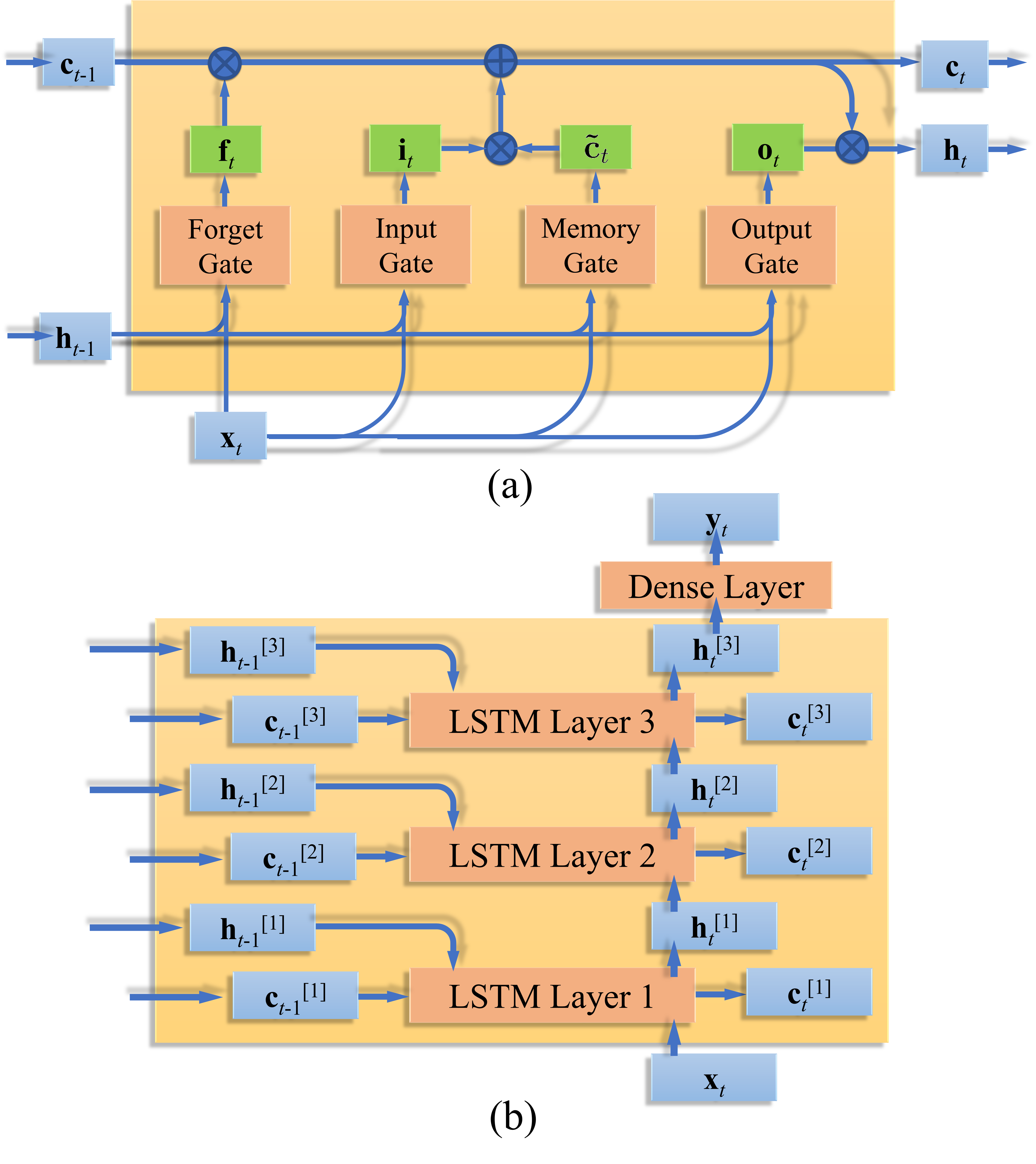
Figure 1: Structures of LSTM unit (a) and multi-layer LSTM networks (b).

In this Letter, we will show that LSTM networks can be incorporated into FSSH to evolve the electronic density matrix. Let us first give a brief review about LSTM. Neural network models represent arbitrary functions with highly interconnected nodes processing through one or several hidden layers. The input vector $\mathbf{x}$ of the function is provided to the nodes in input layer, and the output vector $\mathbf{y}$ is obtained from the nodes in output layer. For a conventional $L$-layer neural network, the connection between two adjacent layers can be expressed as

$$\mathbf{h^{\mathrm{[\mathit{l}]}}} = f\left(\mathbf{W^{\mathrm{[\mathit{l}]}}}\mathbf{h^{\mathrm{[\mathrm{\mathit{l}-1}]}}}+\mathbf{B^{\mathrm{[\mathit{l}]}}}\right)$$ (1)

where $l=1,2,...,L$. In the above equation, the $l$-th layer receives $\mathbf{h^{\mathrm{[\mathrm{\mathit{l}-1}]}}}$ from the previous layer and sends $\mathbf{\mathbf{h^{\mathrm{[\mathit{l}]}}}}$ to the next layer, $\mathbf{\mathbf{W^{\mathrm{[\mathit{l}]}}}}$ and $\mathbf{\mathbf{B^{\mathrm{[\mathit{l}]}}}}$ denote weight and bias parameters for the current layer, respectively, and $f$ is the activation function such as a sigmoid or hyperbolic tangent function. Note that $\mathbf{h^{\mathrm{[\mathrm{0}]}}}=\mathbf{x}$ for input layer and $\mathbf{h^{\mathrm{[\mathrm{\mathit{L}}]}}}=\mathbf{y}$ for output layer. Recurrent neural network takes this form in general but accepts a sequence as input variables. A time series $\mathbf{x}_{1},\mathbf{x}_{2},...,\mathbf{x}_{t}$ is a typical input sequence, in which $\mathbf{x}_{t+1}$ at the next time step can be predicted using neural network as

$$\mathbf{h}_{t} = f_{1}\left(\mathbf{W}_{hx}\mathbf{x}_{t}+\mathbf{W}_{hh}\mathbf{h}_{t-1}+\mathbf{B}_{h}\right)$$ (2)

$$\mathbf{y}_{t} = f_{2}\left(\mathbf{W}_{yh}\mathbf{h}_{t}+\mathbf{B}_{y}\right)$$ (3)

where $\mathbf{W}_{hx}$, $\mathbf{W}_{hh}$ and $\mathbf{W}_{yh}$ are weight parameters, $\mathbf{B}_{h}$ and $\mathbf{B}_{y}$ are bias parameters, $f_{1}$ and $f_{2}$ can be selected as the same or different activation functions, $\mathbf{h}_{t}$ is the hidden state vector that implicitly involves historical information of $\mathbf{x}$, i.e., $\mathbf{x}_{1},\mathbf{x}_{2},...,\mathbf{x}_{t-1}$ through $\mathbf{h}_{t-1}$ (see Eq 2), and $\mathbf{x}_{t+1}$ is identical to or obtained based on the output of neural network ($\mathbf{y}_{t}$). The hidden state and all input vectors at previous time steps are fully-connected in RNN and prone to an exploding or vanishing gradient. The former can be solved using gradient clipping, while the latter can be addressed using a gating mechanism such as long short-term memory networks or gate recurrent unit (GRU). In LSTM, $\mathbf{h}_{t}$ is employed to represent the short-term state, and an additional vector $\mathbf{c}_{t}$ is introduced to preserve the long-term state, which is so-called memory. As shown in Figure 1(a), a gated cell is designed to decide what to store by a forget gate $\mathbf{f}_{t}$ , what to read by an input gate $\mathbf{i}_{t}$, and what to write by an output gate $\mathbf{o}_{t}$; that is

$$\mathbf{f}_{t} = \sigma\left(\mathbf{W}_{fx}\mathbf{x}_{t}+\mathbf{W}_{fh}\mathbf{h}_{t-1}+\mathbf{B}_{f}\right)$$ (4)

$$\mathbf{i}_{t} = \sigma\left(\mathbf{W}_{ix}\mathbf{x}_{t}+\mathbf{W}_{ih}\mathbf{h}_{t-1}+\mathbf{B}_{i}\right)$$ (5)

$$\mathbf{o}_{t} = \sigma\left(\mathbf{W}_{ox}\mathbf{x}_{t}+\mathbf{W}_{oh}\mathbf{h}_{t-1}+\mathbf{B}_{o}\right)$$ (6)

where $\sigma$ denotes the sigmoid function. The propagation of LSTM is given by

$$\mathbf{\tilde{c}}_{t} = \tanh\left(\mathbf{W}_{cx}\mathbf{x}_{t}+\mathbf{W}_{ch}\mathbf{h}_{t-1}+\mathbf{B}_{c}\right)$$ (7)

$$\mathbf{c}_{t} = \mathbf{f}_{t}\varodot\mathbf{c}_{t-1}+\mathbf{i}_{t}\varodot\mathbf{\mathbf{\tilde{c}}}_{t}$$ (8)

$$\mathbf{h}_{t} = \tanh\left(\mathbf{c}_{t}\right)\varodot\mathbf{o}_{t}$$ (9)

Here $\varodot$ denotes the elementwise product, $\mathbf{y}_{t}$ is obtained from $\mathbf{h}_{t}$ via a dense layer using Eq 3 with a hyperbolic tangent function, and $\mathbf{x}_{t+1}$ is identical to or obtained based on $\mathbf{y}_{t}$. Eqs 4-9 can be briefly expressed as

$$\left\{\mathbf{h}_{t},\mathbf{c}_{t}\right\} = LSTM\left(\mathbf{x}_{t},\mathbf{h}_{t-1},\mathbf{c}_{t-1};\mathbf{W},\mathbf{B}\right)$$ (10)

In this work, a multi-layer LSTM is employed and shown in Figure 1(b); that is

$$\left\{\mathbf{h}_{t}^{[l]},\mathbf{c}_{t}^{[l]}\right\} = LSTM\left(\mathbf{h}_{t}^{[l-1]},\mathbf{h}_{t-1}^{[l]},\mathbf{c}_{t-1}^{[l]};\mathbf{W^{\mathrm{[\mathit{l}]}}},\mathbf{\mathbf{B^{\mathrm{[\mathit{l}]}}}}\right)$$ (11)

where $l=1,2,3,$ $\mathbf{h}_{t}^{[0]}=\mathbf{x}_{t}$, and $\mathbf{h}_{t}^{[3]}$ is applied to the dense layer to predict $\mathbf{x}_{t+1}$.

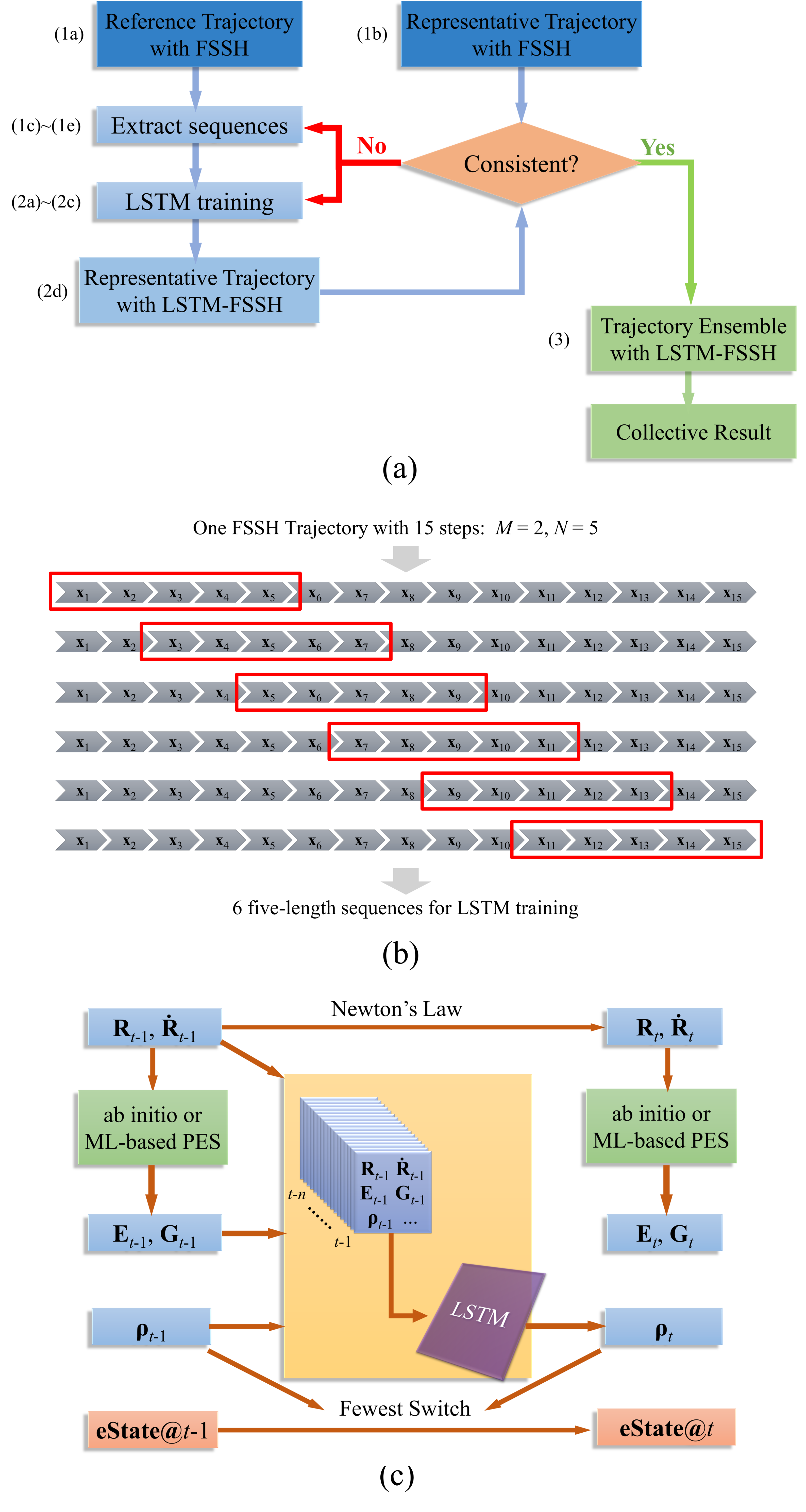
Figure 2: Workflow for LSTM-FSSH: whole procedure with three steps (top), example on generation of sequences from a reference trajectory in step 1 (middle) and implementation on dynamical simulations in step 3 (bottom).

Here we implemented LSTM networks into the original version of FSSH. The extension to a variety of modified surface hopping algorithms is straightforward in principle. In the surface hopping scheme, the nuclear motion is determined by the gradients on a single adiabatic PES; that is

$$M_{a}\mathbf{\ddot{R}}_{a}=-\nabla_{\mathbf{R}_{a}}E_{k}$$ (12)

where $\mathbf{R}_{a}$ and $M_{a}$ denote the position and mass of nucleus $a$, respectively, and $k$ denotes the adiabatic electronic state at the current time step with the relevant potential energy $E_{k}$. The time evolution on electronic subsystem can be expressed as

$$\dot{\rho}_{jk}=-\frac{i}{\hbar}\rho_{jk}\left(E_{j}-E_{k}\right)-\sum_{l}\dot{\mathbf{R}}\cdot\left(\mathbf{d}_{jl}\rho_{lk}-\rho_{jl}\mathbf{d}_{lk}\right)$$ (13)

where $\mathbf{d}_{jk}$ is the nonadiabatic coupling vector between state $j$ and $k$, and $\mathbf{\rho}$ denotes the electronic density matrix. According to the assumption of the fewest number of switches, the probability of nonadiabatic transitions from the current state $k$ to state $j$ in a time interval $\Delta t$ is

$$P_{k\rightarrow j}\left(t,t+\Delta t\right)=\max\left(0,\frac{\int_{t}^{t+\Delta t}2\mathrm{Re}\left(\dot{\mathbf{R}}\cdot\mathbf{d}_{kj}\rho_{jk}\right)d\tau}{\rho_{kk}\left(t\right)}\right)$$ (14)

For a system only involving two electronic states, the probability of switching from the current state $k$ to state $j$ is identical to that of jumping out from state $k$, which can be expressed as¹⁰

$$P_{k\rightarrow j}\left(t,t+\Delta t\right)=\max\left(0,\frac{\rho_{kk}\left(t\right)-\rho_{kk}\left(t+\Delta t\right)}{\rho_{kk}\left(t\right)}\right)$$ (15)

In presence of multiple electronic states, Eq 15 is the summation over hopping probabilities from the current state to all other states and cannot be used directly. During FSSH simulations on molecular systems, however, the hopping is only allowed when the energy gap is lower than a certain threshold (e.g., 10 kcal/mol) in practice. It means that in most regions of PES, the quantum subsystem can be reduced to the simple two-state case. It is no longer reliable in the vicinity of multistate intersections, in which some advanced nonadiabatic dynamical simulations beyond FSSH are usually required.

During conventional FSSH simulations, Eqs 12 and 13 are used to govern nuclear and electronic motion, respectively, and the hopping probability is calculated with Eq 14. In LSTM-FSSH, a LSTM network is built based on a small number of existing trajectories and works as a propagator of electronic degrees of freedom, which replaces Eq 13. In other words, $\mathbf{\mathbf{\rho}}\left(\mathit{t}\mathrm{+\Delta}\mathit{t}\right)$ is predicted by LSTM based on a time series in the preceding trajectory without solving Eq 13. The hopping probability is obtained directly using Eq 15 instead of Eq 14. On one hand, the time evolution on classical subsystem can be also learned by LSTM or RNN as reported in recent works.^{37, 38} On the other hand, several ML-based protocols have been performed excellently to predict accurate potential energies and gradients on the right-hand side of Eq 12, which may be a better choice for realistic molecular systems.^{51, 52} Here the classical subsystem still evolves according to Eq 12 with analytical gradients of our test model systems. More benchmarks and further methodology developments on this issue are left for future work.

The workflow of LSTM-FSSH is summarized in Figure 2. We take a one-dimensional system with two electronic states as an instance and outline the procedure as follows:

Step 1. Database construction.

(1a) Conventional FSSH simulations with a time step $\mathrm{\Delta}\mathit{t}$ are performed to generate a small number of reference trajectories. The nuclear position $\mathbf{R}$ and velocity $\mathbf{\dot{R}}$, potential energies and gradients in two states as $E_{0}$, $E_{1}$, $\mathbf{G}_{0}$, $\mathbf{G}_{1}$, as well as two independent elements of electronic density matrix as $\rho_{00}$ and $\rho_{01}$, are recorded at each step.

(1b) Select a few representative trajectories as “external reference trajectories” in preparation for (2d). For example, three trajectories at a low, medium and high initial momentum for each model are selected in this work. These trajectories are excluded from reference trajectories in (1c)-(2c).

(1c) A time series $\mathbf{x}_{1},\mathbf{x}_{2},...,\mathbf{x}_{N}$ with $N$ frames is extracted with a time step $\mathrm{\Delta}\mathit{t}_{s}$ from one reference trajectory. Here $\mathbf{x}$ consists of $\mathbf{R}$, $\mathbf{\dot{R}}$, $E_{0}$, $E_{1}$, $\mathbf{G}_{0}$, $\mathbf{G}_{1}$, $\rho_{00}$, $\rho_{01}$ and/or arbitrary functions of the above nuclear degrees of freedom, and $\mathrm{\Delta}t_{s}$ is equal to $\mathrm{\Delta}\mathit{t}$ for simplicity.

(1d) The sequence obtained in (1c) is shifted forward by $M$ frames with the same time step to extract another time series until the end of this reference trajectory.

(1e) Repeat (1c) and (1d) on other reference trajectories to extract a large number of $N$-length sequences as the database for LSTM training.

Step 2. LSTM training.

(2a) Select 80% of reference sequences randomly from the database to build the training set. The remaining sequences belong to the testing set.

(2b) Set initial values of hyperparameters of LSTM, such as layer sizes of network and batch sizes for minimization.

(2c) Perform the training of LSTM based on the training set. The mean squared error (MSE) of $\rho_{00}$ and $\rho_{01}$ is minimized using Adam optimizer⁵³, and the MSE for the testing set is monitored to avoid overfitting.

(2d) Perform LSTM-FSSH with the same initial condition and random numbers for hopping of the external reference trajectories selected in (1b). If the generated trajectory visually agrees with the corresponding FSSH trajectory, the present LSTM model is acceptable. Otherwise, return to (2c) to rebuild LSTM using different hyperparameters and random numbers for training.

Step 3. FSSH simulation.

(3a) Initialize the nuclear position, velocity and electronic density matrix for one trajectory as the same as conventional FSSH simulation without machine learning.

(3b) Perform conventional FSSH simulation using Eqs 12, 13 and 14 for $N$ steps to produce an $N$-length sequence, that is, a short-time dynamics in absence of LSTM in the beginning.

(3c) The generated sequence is provided into LSTM to predict electronic density matrix in the next step. Note that the dimensionalities of input and output features of LSTM can be different. Take our test case as an instance. The output layer usually has three nodes as $\rho_{00}$, $\mathrm{Re\left(\rho_{01}\right)}$ and $\mathrm{Im\left(\rho_{01}\right)}$, while the input layer includes all nuclear and electronic features.

(3d) The nuclear position and velocity are propagated to the next step using Eq 12, followed by the calculation on potential energies and gradients in all electronic states. The hopping probability between electronic states is obtained using Eq 15, and the nuclear velocity is adjusted if a switch occurs. This step is the same as conventional FSSH simulation without machine learning, except for the calculation on hopping probability.

(3e) Shift the $N$-length sequence forward by one step. Now the electronic and nuclear features updated in (3c) and (3d) is added into the sequence.

(3f) Return to (3c) to propagate the trajectory until the stopping criterion such as the maximum MD step is achieved.

(3g) Repeat (3a)-(3f) to produce a large number of trajectories. Study collective photodynamic behavior of the system based on trajectory ensemble.

It is worthy noting that step (2d) is the most essential during the whole procedure. Unlike the common case of ML training, step (2c) converges very quickly and seems to be insensitive to hyperparameters in our test case. It indicates that the MSE for the testing set may be insufficient to reflect actual performance of LSTM on dynamical simulations. Actually, it is observed that a set of LSTM networks, all of which perform excellently in (2c), usually produce diverse FSSH trajectories with the same initial condition and random numbers. It may be due to the cumulative error of ML propagator after a long-time ML-driven dynamical simulation. The implementation in step (2d) is thus required. In this work, we compare the time evolution of electronic density matrix visually as a criterion of consistency between external reference and LSTM-FSSH trajectories. The hyperparameters $M$ and $N$ in step 1 are also tuned, leading to a reconstructed database. In practice, the input features as well as the arbitrary functions mentioned in step (1c) may be even necessary to select again before returning to (2c). However, the additional computational cost is small because the reference FSSH trajectories have been produced in step (1a) and keep the same regardless of database reconstruction or input feature reselection.

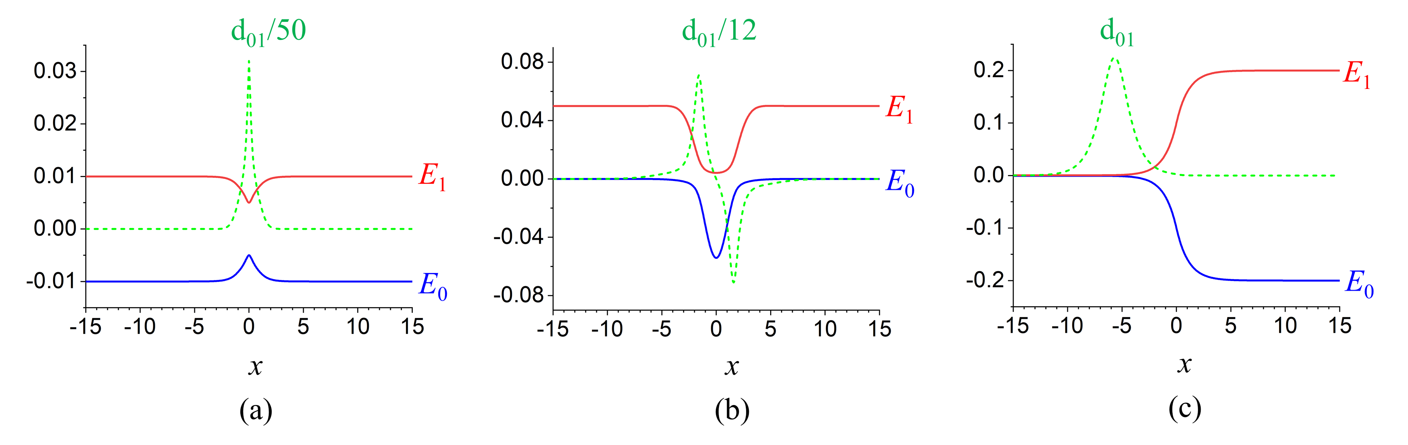
Figure 3: Adiabatic PESs and nonadiabatic coupling vectors of the single-avoided crossing model (a), the dual-avoided crossing model (b), and the extended coupling Hamiltonian model (c). All quantities are in atomic units.

We employ Tully’s three models reported in the original FSSH paper¹⁰: the single-avoided crossing model, the dual-avoided crossing model, and the extended coupling model as our test systems (Fig. 3), which are supposed to cover most of the typical features in realistic molecular systems. The reference trajectories as well as the final collective results for comparison are obtained using the original FSSH method despite its well-known limitations such as the overcoherence problem.^{54, 55, 56, 57} All parameters of Tully’s models are in atomic units. In order to keep consistent with previous works, the classical position $\mathbf{R}$ and velocity $\mathbf{\dot{R}}$ in Fig. 2(c) are represented by $x$ and $v$, respectively, for Tully’s three models. All trajectories start at $x=-20.0$ on the lower surface with an initial momentum to the right and stop at $x=\pm 25.0$. The elements of electronic density matrix are initialized as zero except $\rho_{00}=1.0$. The time step $\mathrm{\Delta}\mathit{t}=1.0$ for all simulations, and $\mathrm{\Delta}t_{s}$ for LSTM is equal to $\mathrm{\Delta}\mathit{t}$. The mass in Eq 12 is set as 2000 to mimic atomic nuclei. For each model and each method, 2000 trajectories are simulated with each initial momentum for collection. The collective results consist of four channels: transmission to $x>25.0$ in the lower state (T1), transmission to $x>25.0$ in the upper state (T2), reflection to $x<-25.0$ in the lower state (R1) and reflection to $x<-25.0$ in the upper state (R2). The proportions that the trajectory stops in each channel are calculated and shown in Fig. 4. The training of all LSTM networks are implemented using Keras⁵⁸ combined with Tensorflow⁵⁹. The interface between FSSH propagator and LSTM networks are built using Keras2C⁶⁰.

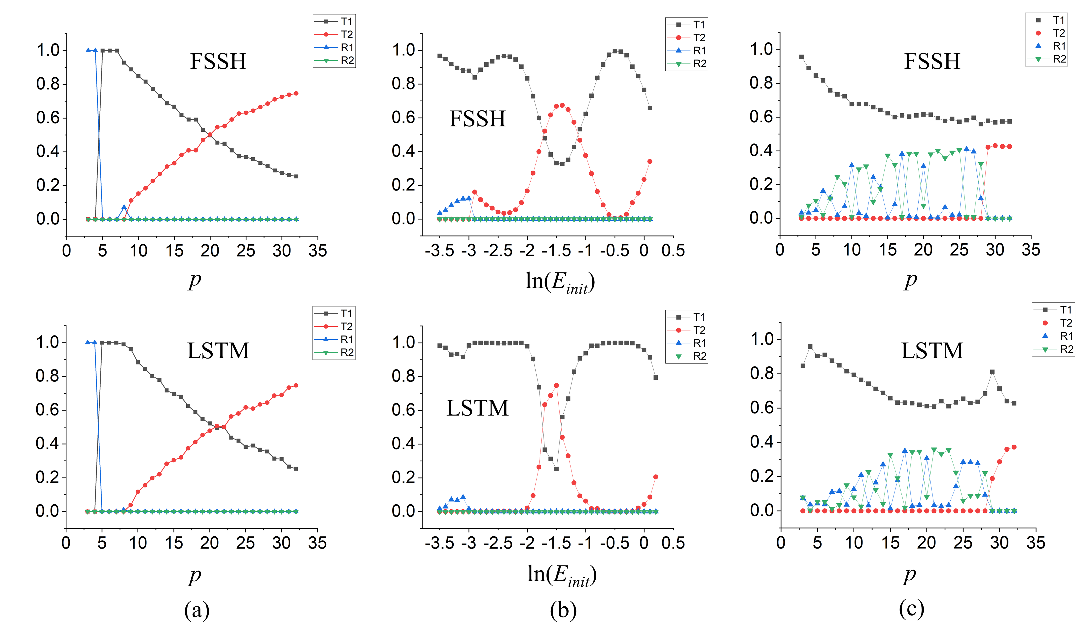
Figure 4: Collective results of single-avoided crossing (a), dual-avoided crossing (b), and extended coupling models (c) obtained using original FSSH as reference (top) or LSTM-FSSH (bottom).

The diabatic Hamiltonian of the single-avoided crossing model is given as

$$V_{11}\left(x\right) = \begin{cases}A\left[1-e^{-Bx}\right]&x>0\\ -A\left[1-e^{Bx}\right]&x<0\end{cases}$$

$$V_{22}\left(x\right) = -V_{11}\left(x\right)$$ (16)

$$V_{12}\left(x\right) = V_{21}\left(x\right)=Ce^{-Dx^{2}}$$

where $A=0.01$, $B=1.6$, $C=0.005$, and $D=1.0$. The corresponding adiabatic PESs and NACVs are shown in Figure 3(a). We generate 20 reference trajectories without machine learning for each initial momentum. The sequences in the training and testing sets are extracted from all reference trajectories with all initial conditions. The classical position $x$, velocity $v$, potential energies $E_{0}$ and $E_{1}$, as well as elements of electronic density matrix are employed as input features. More details can be seen in Tables S1, S2 and S3.

The excellent performance for the testing set in step (2c) is shown in Figure S1. As mentioned in step (2d), LSTM-FSSH simulations are implemented to produce three representative trajectories with different initial momenta. The time evolution of $\rho_{00}$, $\mathrm{Re\left(\rho_{01}\right)}$ and $\mathrm{Im\left(\rho_{01}\right)}$ is compared to the corresponding reference trajectories with the same initial condition and random numbers for hopping (see Figure 5). At a low momentum of 5.0, LSTM-FSSH keeps consistent with the reference for 12500 steps. The deviation takes place after the system departs from the coupling region, which will not affect collective results. At a medium momentum of 15.0 and a large momentum of 30.0, LSTM-FSSH agrees well with the reference except for a slightly fluctuation of $\rho_{00}$ after a sudden decay. The hopping event is observed only at a large momentum. The system switches to the upper surface at step 1882 and 1339 with and without LSTM, respectively. Then we run 2000 trajectories with each initial momentum (60000 in total) using LSTM-FSSH. As shown in Figure 4, the collective result is almost the same as the original FSSH simulations. The resonance phenomenon at $7.0<p<9.0$ populated on R1 can be partially captured by machine learning with a smaller probability.

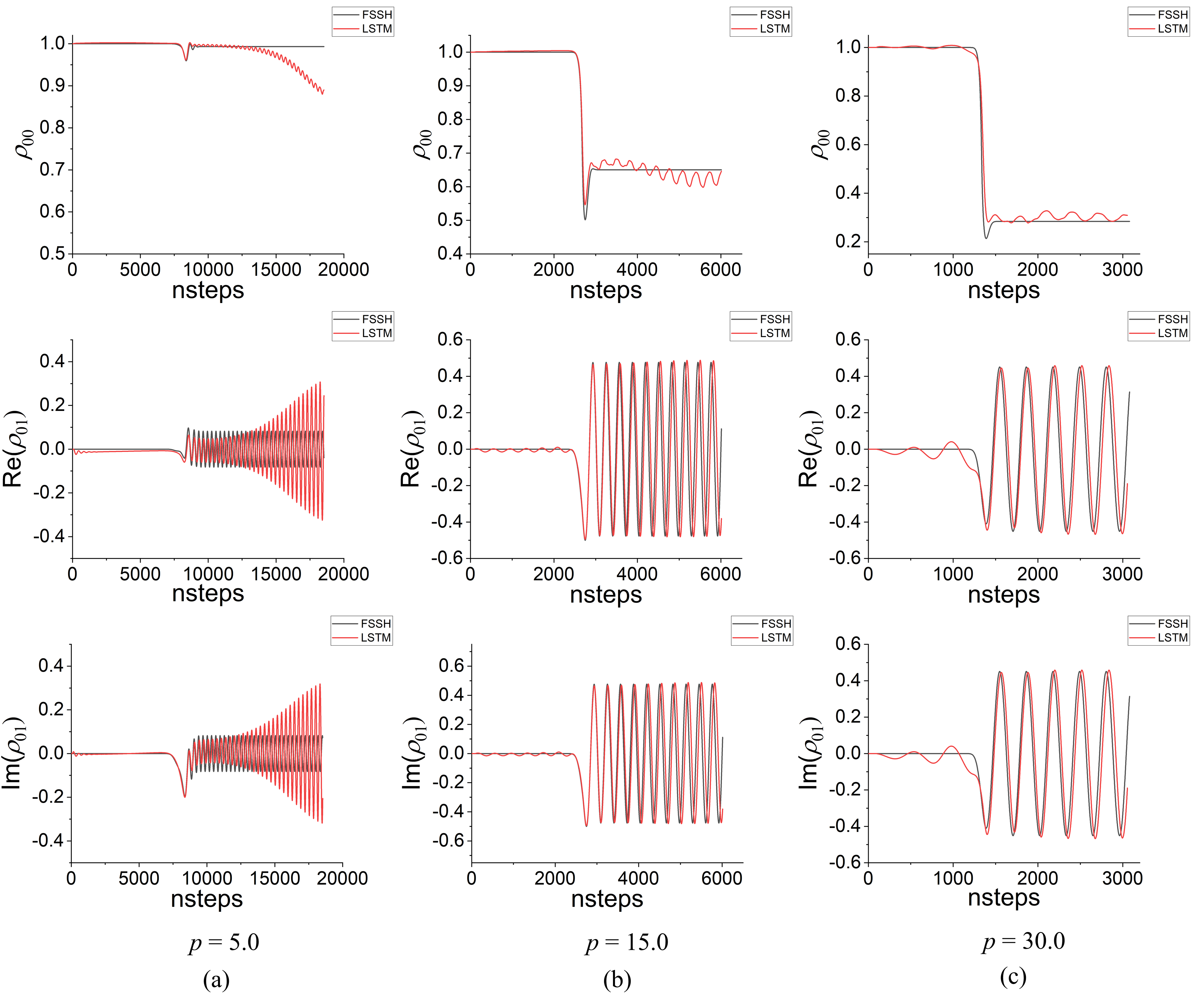
Figure 5: Electronic density matrix plotted as function of time for representative trajectories of single-avoided crossing model at a low (a), medium (b) and high (c) initial momentum. Different colors represent different simulation methods (black: original FSSH as reference; red: LSTM-FSSH).

The diabatic Hamiltonian of the dual-avoided crossing model is

$$V_{11}\left(x\right) = 0$$

$$V_{22}\left(x\right) = -Ae^{-Bx^{2}}+E$$ (17)

$$V_{12}\left(x\right) = V_{21}\left(x\right)=Ce^{-Dx^{2}}$$

where $A=0.10$, $B=0.28$, $C=0.015$, $D=0.06$, and $E=0.05$. The adiabatic PESs and NACVs are shown in Figure 3(b), where $E_{init}$ denotes the initial kinetic energy, and the initial momentum $p=\sqrt{2mE_{init}}$. For each initial momentum, there are 50 reference trajectories generated without machine learning. Then the reference sequences are extracted to build the database for LSTM training, covering all initial momenta. The input features are selected as the same as the first model. More details can be seen in Tables S1, S2 and S4.

First, it can be seen from Figure S1 that the performance for the testing set is remarkable. Second, three representative trajectories using LSTM-FSSH simulations are compared. As shown in Figure 6, the higher the initial momentum, the better the performance of machine learning. At a low momentum of $\ln(E_{init})=-3.0$, LSTM-FSSH deviates away from the reference after step 3000. Both trajectories switch to the upper surface at step 2949, and return to the lower surface at step 4257 and 7156 using LSTM and FSSH, respectively. At a medium momentum of $\ln(E_{init})=-1.5$, two trajectories share the same hopping event at step 1424. At a high momentum of $\ln(E_{init})=-0.5$, the transition between two surfaces is never observed in the representative trajectories using LSTM, while the original FSSH simulation predicts an excited-state population lasting for a short time around step 800. Finally, 2000 LSTM-FSSH trajectories with each initial momentum (74000 in total) are implemented. The collective result shown in Figure 4 is consistent with the performance on representative trajectories. Our method gives a qualitatively correct result except an error within $-3.0<\ln(E_{init})<-2.0$ where the increase of T2 population is missing. It is probably due to the relatively small number of T2 trajectories in our training set, but manually picking trajectories with a specified population is always unrealistic for polyatomic molecules.

The simulation results using another LSTM model with different hyperparameters are reported in Figs. S1, S17 and S18. No problem can be observed from the MSE of the testing set in step (2c). However, the FSSH simulations with and without machine learning in step (2d) represent opposite tendencies of the time evolution of $\rho_{00}$. At a low momentum, $\rho_{00}$ keeps around 1.0 in the reference but decreases to 0.5 using LSTM after a long-time dynamics. At a medium momentum, $\rho_{00}$ converges to 0.3 in the reference but returns to 0.8 using LSTM. It indicates large cumulative errors of this inappropriate LSTM model, leading to an incorrect collective result.

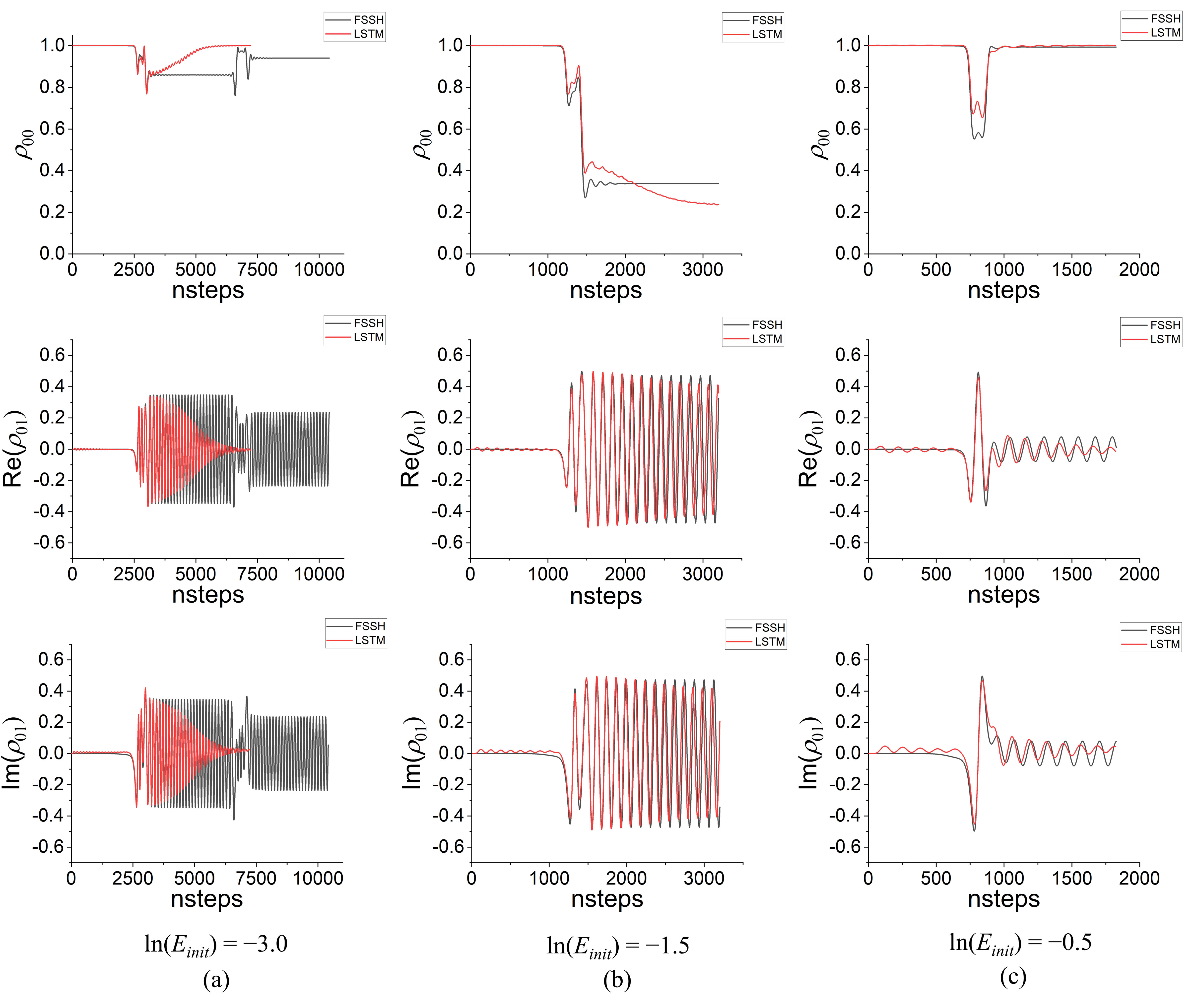
Figure 6: Electronic density matrix plotted as function of time for representative trajectories of dual-avoided crossing model at a low (a), medium (b) and high (c) initial momentum. Different colors represent different simulation methods (black: original FSSH as reference; red: LSTM-FSSH).

The diabatic Hamiltonian of the extended coupling model is

$$V_{11}\left(x\right) = A$$

$$V_{22}\left(x\right) = -A$$ (18)

$$V_{12}\left(x\right) = V_{21}\left(x\right)=\begin{cases}B\left[2-e^{-Cx}\right]&x>0\\ Be^{Cx}&x<0\end{cases}$$

where $A=0.0006$, $B=0.1$, and $C=0.9$. The adiabatic PESs and NACVs are shown in Figure 3(c). Note again that the original FSSH simulation results are employed as the reference of machine learning, and the decoherence correction, which is necessary for this model to reproduce its full-quantum dynamics behavior, is out of our scope in this work. We first implement FSSH simulations without machine learning to produce 50 reference trajectories at each initial momentum. However, all attempts on LSTM training using the above strategy are unsuccessful in step (2d). As shown in Fig. S19, the decrease of $\rho_{00}$ appears too early using LSTM; LSTM also fails to reproduce the strong oscillation of $\rho_{01}$, which is relevant to the coherence in the coupling region. Unsurprisingly, the collective result deviates away from the reference (see Fig. S20).

We refine the LSTM network in two ways. First, since the coupling between quantum and classical subsystems is the key factor of MQC-MD, elaborate selection on input features related to nuclear degrees of freedom is expected to improve the performance of LSTM on the prediction of electronic motion. Functions of nuclear degrees of freedom: $\frac{G_{0}\left|v\right|}{\left(E_{1}-E_{0}\right)^{2}}$ and $\frac{G_{1}\left|v\right|}{\left(E_{1}-E_{0}\right)^{2}}$, are introduced as two additional input features. Three factors including the degeneracy of PESs, the branching of PESs and the correlation between nuclear velocity and transition probability in the intersection region are considered. It would be beneficial to add a small positive bias $\varepsilon$ to denominator when the potential energy difference is very close to zero, but we have never encountered such a problem on numerical instability in the present work. Second, multiple connected LSTM networks are constructed. As shown in Fig. S11(a-d), the first LSTM network is used at the beginning of trajectory ($x=-20.0$). When the system first reaches $x=-2.0$, the second LSTM is employed until it first reaches $x=1.0$ or returns to $-2.0$. The third LSTM is applied sequentially until the system first reaches $x=4.0$ or returns to $-7.0$. The last LSTM is responsible when $x\geq 4.0$ or $\leq-7.0$. Two infrequent cases were also displayed in Fig. S11(e-f), in which the velocity reverses when $x\leq-2.0$ or $\geq 4.0$ at a very low or high momentum, respectively. In the former case, the first LSTM would switch to the third one immediately; in the latter case, the last LSTM would change to the third one when the system returns to $x=4.0$. The third network would be kept until $x\leq-7.0$ in both cases, followed by the last LSTM. More details of LSTM used for the extended coupling model can be seen in Tables S1, S2 and S5.

The comparison between three representative LSTM-FSSH trajectories and their corresponding references is shown in Figure 7. The multiple networks perform well. The time evolution of $\rho_{00}$, $\mathrm{Re}(\rho_{01})$ and $\mathrm{Im}(\rho_{01})$ agrees with the reference except for a problem at a low momentum of 5.0, where $\rho_{00}$ descends too early and tends to oscillate using LSTM. Hopping events are observed only at a medium momentum of 15.0 with both methods, taking place at the same step as 1927. The collective result shown in Figure 4 is obtained from 2000 LSTM-FSSH trajectories with each initial momentum (60000 in total). LSTM-FSSH is qualitatively identical to the original FSSH simulations without machine learning. Further analysis on the distribution of hopping events is shown in Figures S9 and S10, disclosing a few unphysical predictions of LSTM after long-time dynamics. This can be attributed to not only the cumulative errors of ML propagator but also the tendency of LSTM-FSSH to learn the average features of trajectory ensemble, in which trajectories starting from the same initial condition should give different time series due to random hopping events. Despite these intrinsic limitations of our method, their influence on simulation results is possible to evaluate or control at least roughly (see Section S2.3, SI). In addition, the MSEs for the testing sets with all LSTM models are indistinguishable in Figure S1 despite different collective results, which highlights the importance of step (2d) on LSTM training. Using a single LSTM with additional input features only partially improves the performance of collective results (see Section S3.2, SI).

Although the improvement of multiple LSTM networks with additional input features is remarkable, we still suggest simple settings of LSTM networks as the first choice on a new system. First, nuclear positions and velocity, potential energies in two electronic states, and elements of electronic density matrix are recommended as initial input features. More complex descriptor such as $\frac{G_{0}\left|v\right|}{\left(E_{1}-E_{0}\right)^{2}}$ and $\frac{G_{1}\left|v\right|}{\left(E_{1}-E_{0}\right)^{2}}$, which also performs well for other test cases in this work (see Fig. S16), can be introduced when LSTM network with different hyperparameters cannot work in step (2d). Second, a close examination on representative trajectories indicates that the discrepancy between energy degeneration and strong coupling regions may lead to the difficulties on the extended coupling model. According to our experience, however, it is an unusual case for realistic photochemical reactions, which can be identified by detecting the coupling region based on frequent hopping events in reference trajectories. Multiple networks provide an option if all attempts using a single LSTM fail. Different networks can be applied to the detected strong coupling region, the intersection region without strong coupling and other regions with a large energy gap between two states.

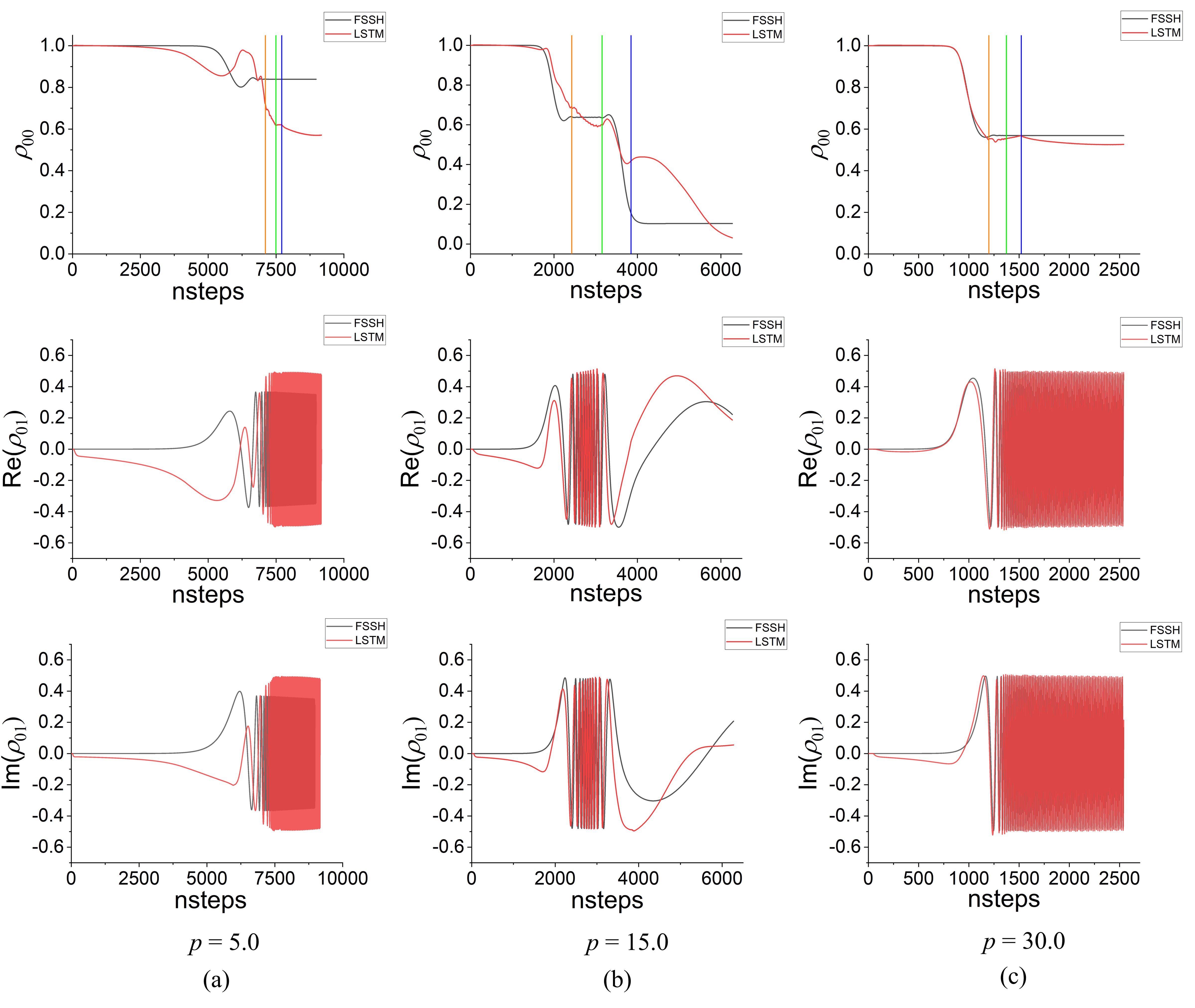
Figure 7: Electronic density matrix plotted as function of time for representative trajectories of extended coupling model at a low (a), medium (b) and high (c) initial momentum. Different colors represent different simulation methods (black: original FSSH as reference; red: LSTM-FSSH). Switches between two connected LSTM networks are represented by vertical lines (orange: $1\mathrm{\rightarrow}2$; green: $2\mathrm{\rightarrow}3$; blue: $3\mathrm{\rightarrow}4$).

The application of this method on realistic molecular systems is attractive, but some nontrivial issues should be addressed in prior. First, although NACV is no longer necessary for two-state systems, the excited-state calculation on potential energies and gradients is still a bottleneck for medium-sized or larger molecules. Fortunately, ML-based force fields have been successfully applied to dynamical simulations on multiple PESs of several organic molecules in photochemistry.^{31, 32, 61, 62, 63} The combination of ML-based force fields and LSTM-FSSH is straightforward, in which the term on the right-hand side of Eq 12 would be obtained from ML prediction instead of electronic structure calculation. Second, the input feature selection is more complicated for high-dimensional classical subsystem. Our preliminary results show that a large number of input features related to nuclear motion hamper the ability of LSTM to propagate electronic subsystem. The encoder network that generates a low-order latent space may be a promising choice to extract more concentrated input features.³⁸ The use of encoder in LSTM-FSSH would be simpler than latent-space classical dynamics because the time evolution on nuclei is still implemented in the full-dimensional space. Third, a general quantitative criterion in step (2d) is absent. Here we compare the representative LSTM-FSSH trajectories with the reference visually, which would be system-specific and laborious for realistic molecules. ML-based analysis of MQC-MD dynamics such as isometric feature mapping and multidimensional scaling provides a possible solution to this trouble.⁶⁴ Fourth, the time-series LSTM predictor always suffers from cumulative errors, while non-time-series ML approaches, which have been implemented for surface hopping dynamics simulations on realistic molecular systems, are free of this problem. More comparisons between LSTM-FSSH and the non-time-series ML-based excited-state dynamics methods such as SchNarc ³⁵ should be performed carefully. Finally, how to extend this method to study the dynamics around multistate intersections is unsolved in this work. We suggest making a pause for ML-driven simulation and switching to a more accurate MQC-MD approach^{7, 65, 66} when the system evolves in multistate intersection regions.

In summary, we have demonstrated how to construct long short-term memory networks as a propagator of electronic subsystem in fewest-switches surface hopping simulations. The single-avoided crossing, dual-avoided crossing and extended coupling models are employed as our test systems. Starting with a small number of full-length trajectories (20-50 for each initial momentum and each model) from the original FSSH simulations, LSTM networks can be built to reproduce the time evolution of electronic density matrix during a long-time FSSH dynamical simulation in presence of only 50-100 steps given as the initial input sequence. Then we simulate 2000 trajectories for each initial momentum and each model using LSTM-FSSH. The collective results is qualitatively consistent with the original FSSH as reference, even though the extended coupling model is much more difficult than other test cases and requires multiple connected LSTM networks. All results show that a lower initial momentum results in a longer-time trajectory with larger cumulative errors, which is an intrinsic drawback of LSTM propagators. Besides avoiding expensive computation on nonadiabatic coupling vectors at least for two-state systems, the combination of LSTM and ML-based force field has a great potential to further accelerate surface hopping simulations on realistic molecular systems. We believe that LSTM is a powerful tool on mixed quantum-classical molecular dynamics to study photophysics and photochemistry more effectively.

Corresponding Author

*Email: lshen@bnu.edu.cn

Supplementary Information

Electronic supplementary information (ESI) including input features and hyperparameters of LSTMs, additional results of LSTM-FSSH, more information on LSTM networks for extended coupling model, and other LSTM networks with unsatisfactory performance is available. The source code is available on https://github.com/TDD365/LSTM-FSSH, under the GNU General Public License v3.0.

See pages - of SI.pdf

References

- Nelson et al. 2020 Nelson, T. R.; White, A. J.; Bjorgaard, J. A.; Sifain, A. E.; Zhang, Y.; Nebgen, B.; Fernandez-Alberti, S.; Mozyrsky, D.; Roitberg, A. E.; Tretiak, S. Non-adiabatic Excited-State Molecular Dynamics: Theory and Applications for Modeling Photophysics in Extended Molecular Materials. Chem. Rev. 2020, 120, 2215–2287
- Prezhdo 2021 Prezhdo, O. V. Modeling Non-adiabatic Dynamics in Nanoscale and Condensed Matter Systems. Acc. Chem. Res. 2021, 54, 4239–4249
- Zobel and González 2021 Zobel, J. P.; González, L. The Quest to Simulate Excited-State Dynamics of Transition Metal Complexes. JACS Au 2021, 1, 1116–1140
- Tully 1998 Tully, J. C. Mixed quantum–classical dynamics. Faraday Discuss. 1998, 110, 407–419
- Stock and Thoss 2005 Stock, G.; Thoss, M. Classical Description of Nonadiabatic Quantum Dynamics. Adv. Chem. Phys. 2005, 131, 243–375
- Curchod et al. 2013 Curchod, B. F. E.; Rothlisberger, U.; Tavernelli, I. Trajectory-Based Nonadiabatic Dynamics with Time-Dependent Density Functional Theory. ChemPhysChem 2013, 14, 1314–1340
- Crespo-Otero and Barbatti 2018 Crespo-Otero, R.; Barbatti, M. Recent Advances and Perspectives on Nonadiabatic Mixed Quantum–Classical Dynamics. Chem. Rev. 2018, 118, 7026–7068
- Gao et al. 2018 Gao, L.-H.; Xie, B.-B.; Fang, W.-H. Theories and Applications of Mixed Quantum-Classical Non-adiabatic Dynamics. Chin. J. Chem. Phys. 2018, 31, 12–26
- Mai and González 2020 Mai, S.; González, L. Molecular Photochemistry: Recent Developments in Theory. Angew. Chem. Int. Ed. 2020, 59, 16832–16846
- Tully 1990 Tully, J. C. Molecular dynamics with electronic transitions. J. Chem. Phys. 1990, 93, 1061–1071
- Hammes-Schiffer and Tully 1994 Hammes-Schiffer, S.; Tully, J. C. Proton transfer in solution: Molecular dynamics with quantum transitions. J. Chem. Phys. 1994, 101, 4657–4667
- Shen et al. 2020 Shen, L.; Xie, B.; Li, Z.; Liu, L.; Cui, G.; Fang, W.-H. Role of Multistate Intersections in Photochemistry. J. Phys. Chem. Lett. 2020, 11, 8490–8501
- Zobel et al. 2021 Zobel, J. P.; Heindl, M.; Plasser, F.; Mai, S.; González, L. Surface Hopping Dynamics on Vibronic Coupling Models. Acc. Chem. Res. 2021, 54, 3760–3771
- Xie et al. 2022 Xie, B.-B.; Jia, P.-K.; Wang, K.-X.; Chen, W.-K.; Liu, X.-Y.; Cui, G. Generalized Ab Initio Nonadiabatic Dynamics Simulation Methods from Molecular to Extended Systems. J. Phys. Chem. A 2022, 126, 1789–1804
- Mukherjee et al. 2022 Mukherjee, S.; Pinheiro, M.; Demoulin, B.; Barbatti, M. Simulations of molecular photodynamics in long timescales. Phil. Trans. R. Soc. A 2022, 380, 20200382
- Raccuglia et al. 2016 Raccuglia, P.; Elbert, K. C.; Adler, P. D. F.; Falk, C.; Wenny, M. B.; Mollo, A.; Zeller, M.; Friedler, S. A.; Schrier, J.; Norquist, A. J. Machine-learning-assisted materials discovery using failed experiments. Nature 2016, 533, 73–76
- Coley et al. 2019 Coley, C. W. et al. A robotic platform for flow synthesis of organic compounds informed by AI planning. Science 2019, 365, eaax1566
- Zhou et al. 2020 Zhou, Q.; Lu, S.; Wu, Y.; Wang, J. Property-Oriented Material Design Based on a Data-Driven Machine Learning Technique. J. Phys. Chem. Lett. 2020, 11, 3920–3927
- Zhang et al. 2020 Zhang, J.; Lei, Y.-K.; Zhang, Z.; Chang, J.; Li, M.; Han, X.; Yang, L.; Yang, Y. I.; Gao, Y. Q. A Perspective on Deep Learning for Molecular Modeling and Simulations. J. Phys. Chem. A 2020, 124, 6745–6763
- Dral 2020 Dral, P. O. Quantum Chemistry in the Age of Machine Learning. J. Phys. Chem. Lett. 2020, 11, 2336–2347
- Smith et al. 2017 Smith, J. S.; Isayev, O.; Roitberg, A. E. ANI-1: an extensible neural network potential with DFT accuracy at force field computational cost. Chem. Sci. 2017, 8, 3192–3203
- Chmiela et al. 2018 Chmiela, S.; Sauceda, H. E.; Müller, K.-R.; Tkatchenko, A. Towards exact molecular dynamics simulations with machine-learned force fields. Nat. Commun. 2018, 9, 3887
- Schütt et al. 2018 Schütt, K. T.; Sauceda, H. E.; Kindermans, P.-J.; Tkatchenko, A.; Müller, K.-R. SchNet – A deep learning architecture for molecules and materials. J. Chem. Phys. 2018, 148, 241722
- Shen and Yang 2018 Shen, L.; Yang, W. Molecular Dynamics Simulations with Quantum Mechanics/Molecular Mechanics and Adaptive Neural Networks. J. Chem. Theory Comput. 2018, 14, 1442–1455
- Zhang et al. 2018 Zhang, L.; Han, J.; Wang, H.; Car, R.; E, W. Deep Potential Molecular Dynamics: A Scalable Model with the Accuracy of Quantum Mechanics. Phys. Rev. Lett. 2018, 120, 143001
- Unke and Meuwly 2019 Unke, O. T.; Meuwly, M. PhysNet: A Neural Network for Predicting Energies, Forces, Dipole Moments, and Partial Charges. J. Chem. Theory Comput. 2019, 15, 3678–3693
- Dral 2019 Dral, P. O. MLatom: A program package for quantum chemical research assisted by machine learning. J. Comput. Chem. 2019, 40, 2339–2347
- Behler 2021 Behler, J. Four Generations of High-Dimensional Neural Network Potentials. Chem. Rev. 2021, 121, 10037–10072
- Zhu and Nakamura 1994 Zhu, C.; Nakamura, H. Theory of nonadiabatic transition for general two-state curve crossing problems. I. Nonadiabatic tunneling case. J. Chem. Phys. 1994, 101, 10630–10647
- Zhu and Nakamura 1995 Zhu, C.; Nakamura, H. Theory of nonadiabatic transition for general two-state curve crossing problems. II. Landau–Zener case. J. Chem. Phys. 1995, 102, 7448–7461
- Hu et al. 2018 Hu, D.; Xie, Y.; Li, X.; Li, L.; Lan, Z. Inclusion of Machine Learning Kernel Ridge Regression Potential Energy Surfaces in On-the-Fly Nonadiabatic Molecular Dynamics Simulation. J. Phys. Chem. Lett. 2018, 9, 2725–2732
- Chen et al. 2018 Chen, W.-K.; Liu, X.-Y.; Fang, W.-H.; Dral, P. O.; Cui, G. Deep Learning for Nonadiabatic Excited-State Dynamics. J. Phys. Chem. Lett. 2018, 9, 6702–6708
- Dral et al. 2018 Dral, P. O.; Barbatti, M.; Thiel, W. Nonadiabatic Excited-State Dynamics with Machine Learning. J. Phys. Chem. Lett. 2018, 9, 5660–5663
- Westermayr et al. 2019 Westermayr, J.; Gastegger, M.; Menger, M. F. S. J.; Mai, S.; González, L.; Marquetand, P. Machine learning enables long time scale molecular photodynamics simulations. Chem. Sci. 2019, 10, 8100–8107
- Westermayr et al. 2020 Westermayr, J.; Gastegger, M.; Marquetand, P. Combining SchNet and SHARC: The SchNarc Machine Learning Approach for Excited-State Dynamics. J. Phys. Chem. Lett. 2020, 11, 3828–3834
- Westermayr and Marquetand 2020 Westermayr, J.; Marquetand, P. Machine Learning for Electronically Excited States of Molecules. Chem. Rev. 2020, 121, 9873–9926
- Wang et al. 2020 Wang, J.; Li, C.; Shin, S.; Qi, H. Accelerated Atomic Data Production in Ab Initio Molecular Dynamics with Recurrent Neural Network for Materials Research. J. Phys. Chem. C 2020, 124, 14838–14846
- Vlachas et al. 2021 Vlachas, P. R.; Zavadlav, J.; Praprotnik, M.; Koumoutsakos, P. Accelerated Simulations of Molecular Systems through Learning of Effective Dynamics. J. Chem. Theory Comput. 2021, 18, 538–549
- Kadupitiya et al. 2022 Kadupitiya, J. C. S.; Fox, G. C.; Jadhao, V. Solving Newton’s equations of motion with large timesteps using recurrent neural networks based operators. Mach. Learn.: Sci. Technol. 2022, 3, 025002
- Winkler et al. 2022 Winkler, L.; Müller, K.-R.; Sauceda, H. E. High-fidelity molecular dynamics trajectory reconstruction with bi-directional neural networks. Mach. Learn.: Sci. Technol. 2022, 3, 025011
- Bandyopadhyay et al. 2018 Bandyopadhyay, S.; Huang, Z.; Sun, K.; Zhao, Y. Applications of neural networks to the simulation of dynamics of open quantum systems. Chem. Phys. 2018, 515, 272–278
- Rodríguez and Kananenka 2021 Rodríguez, L. E. H.; Kananenka, A. A. Convolutional Neural Networks for Long Time Dissipative Quantum Dynamics. J. Phys. Chem. Lett. 2021, 12, 2476–2483
- Reh et al. 2021 Reh, M.; Schmitt, M.; Gärttner, M. Time-Dependent Variational Principle for Open Quantum Systems with Artificial Neural Networks. Phys. Rev. Lett. 2021, 127, 230501
- Lin et al. 2021 Lin, K.; Peng, J.; Gu, F. L.; Lan, Z. Simulation of Open Quantum Dynamics with Bootstrap-Based Long Short-Term Memory Recurrent Neural Network. J. Phys. Chem. Lett. 2021, 12, 10225–10234
- Ullah and Dral 2021 Ullah, A.; Dral, P. O. Speeding up quantum dissipative dynamics of open systems with kernel methods. New J. Phys. 2021, 23, 113019
- Ullah and Dral 2022 Ullah, A.; Dral, P. O. Predicting the future of excitation energy transfer in light-harvesting complex with artificial intelligence-based quantum dynamics. Nat. Commun. 2022, 13, 1930
- Secor et al. 2021 Secor, M.; Soudackov, A. V.; Hammes-Schiffer, S. Artificial Neural Networks as Propagators in Quantum Dynamics. J. Phys. Chem. Lett. 2021, 12, 10654–10662
- Yang et al. 2020 Yang, B.; He, B.; Wan, J.; Kubal, S.; Zhao, Y. Applications of neural networks to dynamics simulation of Landau-Zener transitions. Chem. Phys. 2020, 528, 110509
- Gao et al. 2021 Gao, L.; Sun, K.; Zheng, H.; Zhao, Y. A Deep-Learning Approach to the Dynamics of Landau–Zenner Transitions. Adv. Theory Simul. 2021, 4, 2100083
- Wu et al. 2021 Wu, D.; Hu, Z.; Li, J.; Sun, X. Forecasting nonadiabatic dynamics using hybrid convolutional neural network/long short-term memory network. J. Chem. Phys. 2021, 155, 224104
- Behler 2017 Behler, J. First Principles Neural Network Potentials for Reactive Simulations of Large Molecular and Condensed Systems. Angew. Chem. Int. Ed. 2017, 56, 12828–12840
- Pinheiro et al. 2021 Pinheiro, M.; Ge, F.; Ferré, N.; Dral, P. O.; Barbatti, M. Choosing the right molecular machine learning potential. Chem. Sci. 2021, 12, 14396–14413
- Kingma and Ba 2015 Kingma, D. P.; Ba, J. Adam: A Method for Stochastic Optimization. 3rd International Conference on Learning Representations ICLR 2015-Conference Track Proceedings; ICLR 2015,
- Nelson et al. 2013 Nelson, T.; Fernandez-Alberti, S.; Roitberg, A. E.; Tretiak, S. Nonadiabatic excited-state molecular dynamics: Treatment of electronic decoherence. J. Chem. Phys. 2013, 138, 224111
- Subotnik et al. 2016 Subotnik, J. E.; Jain, A.; Landry, B.; Petit, A.; Ouyang, W.; Bellonzi, N. Understanding the Surface Hopping View of Electronic Transitions and Decoherence. Annu. Rev. Phys. Chem. 2016, 67, 387–417
- Plasser et al. 2019 Plasser, F.; Mai, S.; Fumanal, M.; Gindensperger, E.; Daniel, C.; González, L. Strong Influence of Decoherence Corrections and Momentum Rescaling in Surface Hopping Dynamics of Transition Metal Complexes. J. Chem. Theory Comput. 2019, 15, 5031–5045
- Tang et al. 2021 Tang, D.; Shen, L.; Fang, W.-H. Evaluation of mixed quantum-classical molecular dynamics on cis-azobenzene photoisomerization. Phys. Chem. Chem. Phys. 2021, 23, 13951–13964
- Chollet et al. 2015 Chollet, F., et al. Keras. 2015; \urlhttps://keras.io
- Abadi et al. 2015 Abadi, M. et al. TensorFlow: Large-Scale Machine Learning on Heterogeneous Systems. 2015; \urlhttps://www.tensorflow.org/
- Conlin et al. 2021 Conlin, R.; Erickson, K.; Abbate, J.; Kolemen, E. Keras2c: A library for converting Keras neural networks to real-time compatible C. Eng. Appl. Artif. Intell. 2021, 100, 104182
- Menger et al. 2020 Menger, M. F. S. J.; Ehrmaier, J.; Faraji, S. PySurf: A Framework for Database Accelerated Direct Dynamics. J. Chem. Theory Comput. 2020, 16, 7681–7689
- Li et al. 2021 Li, J.; Stein, R.; Adrion, D. M.; Lopez, S. A. Machine-Learning Photodynamics Simulations Uncover the Role of Substituent Effects on the Photochemical Formation of Cubanes. J. Am. Chem. Soc. 2021, 143, 20166–20175
- Lin et al. 2021 Lin, S.; Peng, D.; Yang, W.; Gu, F. L.; Lan, Z. Theoretical studies on triplet-state driven dissociation of formaldehyde by quasi-classical molecular dynamics simulation on machine-learning potential energy surface. J. Chem. Phys. 2021, 155, 214105
- Li et al. 2017 Li, X.; Xie, Y.; Hu, D.; Lan, Z. Analysis of the Geometrical Evolution in On-the-Fly Surface-Hopping Nonadiabatic Dynamics with Machine Learning Dimensionality Reduction Approaches: Classical Multidimensional Scaling and Isometric Feature Mapping. J. Chem. Theory Comput. 2017, 13, 4611–4623
- Curchod and Martínez 2018 Curchod, B. F. E.; Martínez, T. J. Ab Initio Nonadiabatic Quantum Molecular Dynamics. Chem. Rev. 2018, 118, 3305–3336
- Shen et al. 2019 Shen, L.; Tang, D.; Xie, B.; Fang, W.-H. Quantum Trajectory Mean-Field Method for Nonadiabatic Dynamics in Photochemistry. J. Phys. Chem. A 2019, 123, 7337–7350